1

Childhood Investments in Human Capital:

Parental Resources and Preferences

Sonia Bhalotra*

Abstract

This paper investigates the way in which parental human capital investment in young

co-resident children varies with their own consumption and leisure. It is motivated by

rejection of parental altruism in recent research, the unexpectedly small effects of

parental income on child outcomes found in a number of studies, and the claim in

several historical and anthropological studies of child labour that parents are selfish.

The results suggest that, in the preference function of parents, child schooling is a

normal good and that child labour is a bad, consistent with altruism. I also test the

income pooling prediction of the unitary model and find that I cannot reject it; there is

no evidence that the consumption of children is increasing in their labour supply.

Keywords: altruism, m-demands, intra-household allocation, human capital, child

labour, education.

JEL codes: C2 I2 O1 R2

*Department of Economics, University of Bristol, 8 Woodland Road, Bristol BS8

1TN, UK. Tel +44 117 928 8418. Email: s.bhalotra@bristol.ac.uk. Also, Research

Fellow IZA (Bonn), CHILD (Turino) and Wolfson College (Cambridge), Research

Associate Centre for Study of African Economies (Oxford) and Queen Elizabeth

House (Oxford), Member CMPO and International Poverty Centre (Bristol).

2

Childhood Investments in Human Capital:

Parental Resources and Preferences

Sonia Bhalotra, University of Bristol (UK)*

1 Introduction

In his survey of theories of intrahousehold allocation, Behrman (1997: p.132)

observes that “parents who are insufficiently wealthy or insufficiently altruistic fail to

provide their children with the socially efficient wealth-maximising level of human

resources.” While many previous studies have argued that sub-optimal levels of

human capital investment can be explained by credit constraints (e.g. Loury 1981,

Parish and Willis 1993, Ranjan 2001, Baland and Robinson 2000, Edmonds 2003),

much less attention has been directed, in this context, at the role of parental

preferences (though see Banerjee 2003, for a theoretical discussion).1 Models of

educational investment and child labour typically assume parent altruism (e.g. Becker

and Tomes 1986, Dessy and Pallage 2001, Basu and Van 1998, Baland and Robinson

2000). But when parents decide how much to spend on the human capital of their

children and the rewards accrue to the child, and over a long horizon, there is an

evident agency issue (e.g. Baland and Robinson 2000).

Childhood is the time when critical investments in human capital are made

that have far-reaching and often irreversible effects on future life-chances. In

developing countries, where public provision is limited, parental preferences and

resources play an especially important role. Evidence of limited parental altruism

would lend weight to legislative interventions such as bans on child labour and

compulsory schooling laws, and it would challenge the efficacy of unconditional cash

transfers. Cash transfer programmes are increasingly popular amongst interventions

* I am grateful to Martin Browning, Christian Dustmann, Sylvain Dessy, Andrew Foster, Chris Heady, Saqib Jaffrey, Steve Nickell, Ian Preston, Ken Swinnerton and Alessandro Tarozzi for helpful comments. The paper has benefited from presentation at the NEUDC Meetings in Boston (Sept 2001), the AEA/AESM Meetings in Atlanta (Jan 2002) and seminars at the Research Department of the World Bank (Mar 2002), George Washington University (Mar 2002), the LSE (STICERD: May 2002), Bristol (Nov 2001), Cambridge (Sep 2001), Sussex/IDS (Nov 2001), the Indian Statistical Institute in Delhi (Dec 2001), and the Centre for Applied Microeconomics in Copenhagen (June 2004). 1 Rogers and Swinnerton (2003) cite the historical research of Parsons and Goldin (1989) and an earlier version of this paper (Bhalotra 2001) as being the only available empirical studies that attempt to examine parental altruism in the context of child labour and schooling.

3

conducted by governments and international organizations in developing countries,

many of which carry the objective of increasing school attendance and reducing child

labour (e.g., the Food for Education Program in Bangladesh, Progresa in Mexico,

Bolsa Escola in Brazil). The fact that, in many cases, the cash transfer is conditional

upon attendance at school or health clinics suggests that concern about possible

“leakages” is recognized on the field (Becker 1999).

This paper tests the first-order condition common to most theoretical models

in the literature, in which altruism is assumed. According to this, moving a child into

work is associated with a decrease in the consumption (or leisure) of parents. The idea

is that parents will equate the marginal utility of their consumption to the marginal

utility of child leisure (which is higher if children work). If this condition holds then

we can reject the hypothesis that parents are selfish or exploitative. It is also

interesting to quantify the trade-offs involved. The paper estimates m-demands, which

describe the indifference curve between adult consumption and child labour. In this

way I directly estimate the ratio of income effects on child labour and adult

consumption. Following a closely related literature, expenditure on adult consumption

is instrumented with a cubic in income, and I follow Moreira (2002) to obtain tests

that yield the correct rejection probabilities for the specifications in which the

instruments are weak.

The data analysed are a household survey for rural Pakistan, a poor society in

which human capital investment in children is low and poverty and market

imperfections impact most households. I find no support for the view that parental

exploitation drives child labour; both child leisure and schooling appear as normal

goods in the parental utility function. Specifically, a 10% increase in adult clothing

expenditure is associated with about a 6 percent point increase in the proportion of

children in the household that attend school, or a 3 percent point decrease in the

proportion of children in work. This result is robust to conditioning upon adult labour.

Pairs of Marshallian demands provide point estimates that are larger but not

significantly different from the m-demand estimates. If I use tobacco expenditure

rather than expenditure on adult clothing as the reference good, then I find a seeming

anomaly: child labour is invariant to increases in tobacco expenditure. At the same

time, increases in tobacco expenditure are associated with increases in schooling. I

argue that the results are reconciled if selection into smoking (non-zero tobacco

expenditure) is correlated with unobservables in the equation for child labour (see

4

section 4.2). Further analysis shows that children are less well-off in households that

have at least one smoker.

Previous studies of intergenerational altruism effectively test income pooling

(see Altonji et al 1992, 1997, Hayashi 1995).2 The condition I test, of positive

transfers, is weaker. However, I extend the analysis to further investigate income

pooling by regressing child clothing expenditure on child labour, holding constant

total expenditure and adult labour. I cannot reject income pooling: expenditure on

children is not increasing in their labour (also see Moehling 2004, Bhalotra and

Attfield 1998).

This research faces two potential challenges. First, that it establishes a result

that is trivial or evident and, second, that it is unable to distinguish between

investments in children that are motivated by reciprocity rather than by altruism. I

now defend it against these concerns, in turn.

In a largely unnoticed challenge to the prevalent assumption in the human

capital literature, numerous historical and anthropological studies of child labour have

cast parents as selfish, sending their children to work to further the ir own

consumption, or to pay off their debts.3 Using US and Japanese data, direct tests of

intergenerational altruism have tended to reject it (see Cox and Rank 1992, Altonji et

al 1992, 1997, Hayashi 1995). In their analysis of child benefit in the UK, Blow,

Walker and Zhu (2004) find that it is spent disproportionately on alcohol. Micro-

econometric research has found some surprisingly small effects of parental income on

child labour (see Rogers and Swinnerton (2004), Bhalotra and Tzannatos (2003),

Brown et al (2003), for example) and schooling (e.g. Behrman and Knowles 1999).

Small effects of parental income on child outcomes have been also been noted in

other contexts (e.g., Shea 2000, Mayer 1997, Currie 1995, Haveman and Wolfe 1995:

p.1856). Overall, it is not evident that improvements in family income are shared with

children so that their leisure or schooling increases. This paper delivers estimates of

2 It is straightforward to show that the income transfer derivative restriction investigated in, for example, Altonji et al 1997, holds only if income pooling holds. Although it is clear in the wider literature that altruism does not imply income pooling and that income pooling can hold in the absence of altruism, available tests of intergenerational altruism are effectively tests of income pooling. 3 Among economic historians, see Parsons and Goldin (1989) and Nardinelli (1990, p. 94), with reference to nineteenth century USA and England respectively. See Khan (2001) for anthropological work on contemporary Sialkot in Pakistan; see Burra (1995), Bhatty (1998)

5

how income is allocated within the household between child leisure (or schooling)

and adult consumption. In the altruistic model, this corresponds to the relative weight

that parents place on the child good.

This paper neglects the issue of altruism versus investment that has been

central in research on transfers between parents and adult children who live in

separate homes, mostly in the US (e.g. Cox and Rank 1992, Laitner 1997). Consistent

with its focus on child labour in poor liquidity-constrained households, it instead

considers altruism versus exploitation in the context of human capital investment in

children who are co-resident minors. The eventual question of interest here is whether

low levels of human capital in developing countries can be attributed to parents failing

to attach any weight to schooling, for whatever reason. Whether or not children

reciprocate when they are older is not of direct interest here since, at the time when

parents are making investment decisions, they cannot contract their children to make

these return transfers (further discussion is in section 2.2).

Section 2 describes the analytical framework and section 3 describes the data

and estimation issues. The main results are presented in section 4. Section 5

investigates robustness to alternative specifications, and section 6 concludes.

2 An Analytical Framework

The prediction of the altruistic model that is tested is set out in section 2.1, where it is

shown to flow from a general class of models in the literature. Section 2.2 argues that

the competing hypothesis that parental human capital investments in children are

motivated by anticipation of reciprocal transfers in old age is not compelling and,

more important, not relevant to the objectives of this paper. M-demands are

introduced in section 2.3 as a useful way of estimating the relationship of interest, and

section 2.4 shows that this is equivalent to estimating the marginal effect of income on

the child outcome, relative to the marginal effect of income on adult consumption.

Previous research has tended to interpret income effects on schooling or child labour

as indicating credit constraints, (implicitly) maintaining the assumption of parental

altruism. It is argued that one could equally maintain the assumption that credit

constraints bind and interpret absent income effects in terms of (absent) altruism.

and Gupta (2000) for field-based research that is consistent with parental selfishness in India; and Fyfe (1989, p.76).

6

2.1 The hypothesis

Suppose that the (period-1) utility function of the parent is AαHβLγCθ, where A

refers to (above-subsistence) adult consumption, H refers to child human capital

(schooling), L is child labour, and C refers to all other consumption, assumed to be

shared. To the extent that child labour reduces schooling, this is reflected in H. The

appearance of L in the utility function allows for a separate role for child leisure, or

for parents to derive disutility from seeing their children work (as in Bommier and

Dubois 2003). It follows directly from the standard optimization programme that

∂H/∂A=(β/α)(pA/pH)>0, where pA, pH are prices of A and H. Similarly, ∂L/∂A<0.4 The

estimates will, of course, confirm whether or not child labour is a “bad”, and to what

extent child labour and schooling are substitutes. Under the null of egoistic parents,

when neither of H and L appear in the parental utility function, ∂H/∂A=0 and, since

child labour augments income, ∂L/∂A≥0.5 This is the condition that is tested.

Basu and Van (1998) set out a simple single-period model in which a critical

assumption is that parents are altruistic and only send their children to work if this is

essential to the survival needs of the household. Clearly, this implies no above-

subsistence consumption in households with child labour. The condition tested in this

paper flows from a more general description of parental altruism, which involves

parents attaching a positive weight to child schooling and a negative weight to child

labour. Baland and Robinson develop a 2-period model in which child labour in

period 1 reduces schooling attainment and, thereby, earnings capacity in period 2. In

period 1, the parent decides the allocation of child time. In period 2, the child decides

whether to make a transfer to the parent and the parent decides how much to consume

and how much to leave the child in bequests.6 The first order conditions of this model

shows that the level of human capital investment in period 1 will co-vary with the

4 For this simple illustration, I have described parental preferences as depending directly on the level of human capital of the child in period-1. This is sometimes referred to as the warm-glow formulation (e.g. Banerjee 2003). The testable predictions that we are concerned with in this paper are unchanged if, instead, the caring representation of preferences (e.g. Bourguignon et al 1994) is used, in which parent utility depends upon child utility, as long as child utility is increasing in H and decreasing in L. 5 The first version of this paper sets out a more general model that includes the consumption and labour supplies of parent and child (Bhalotra 2001). Although here I discuss how child labour varies with adult consumption, below I also consider how it varies with adult labour supply. 6 The labour supply of parents is assumed exogenous in these models. This assumption is relaxed in the empirical analysis in this paper.

7

level of parental consumption in period 1. This is the condition tested in this paper. If,

instead, parents were selfish and neither cared about child utility nor derived a “warm

glow” from the level of human capital of their children, then additional income would

be spent on parental consumption (or leisure) without necessarily incrementing the

level of human capital of their children (the case of a horizontal income expansion

path). Similarly, if parental utility depends upon child utility, or if child labour

directly generates disutility for the parent, the FOCs will imply a negative relation of

child labour and parental consumption. Any increment in income will be used to

simultaneously buy more parental consumption and reduce child labour (in line with

the MRS condition). This condition is also tested.

Some existing research has investigated whether, when children work,

incomes are pooled (Bhalotra and Attfield 1998, Moehling 2004). This research is

motivated by the idea that income-shares of family members are associated with

bargaining power and therefore with resource claims. But the prior question is: Why

do children work? To understand this, it is relevant to consider whether parents cut

back their own above-subsistence consumption or leisure in order to avoid the child

working. No previous research has attempted to investigate this.

2.2 Altruism vs exchange motives

The previous section describes a testable prediction of the altruistic model. Finding

that the data satisfy that prediction is, as always, potentially consistent with other

hypotheses. The main competing hypothesis here is that of exchange: parents may

send their children to school rather than to work not because they are altruistic but

because they expect that a higher level of investment in child human capital in period-

1 will bring them higher return transfers in period-2 (e.g. Nugent 1985, Cox 1987,

Lillard and Willis 1997).

The exchange motive is undermined by the fact that it is difficult for parents to

enforce repayment from children, especially over a long horizon (e.g. Baland and

Robinson 2000, Fitzsimmons 2003).7 Moreover, the evidence on the exchange motive

is not compelling. Although positive evidence is reported in Lillard and Willis (1997)

7 Fitzsimons emphasizes that even where there are ad hoc transfers from child to parent in period 2, what is important is that, when parents are making human capital decisions in period 1, they know that reciprocity is not enforceable. Although Lopez-Calva and Miyamoto (2004)

8

and Lucas and Stark (1995), Kochar (2000), Fitzsimons (2003) and Pal (2004) find

little support for the hypothesis that the probability or amount of transfers received by

elderly parents is increasing in the leve l of education of their children. The distinction

between altruism and exchange may, further, be seen as inherently impossible to

make. Thus, even when the child’s utility is an argument in the parental utility

function, parents are maximizing their own utility and, by that criterion, may be

regarded as selfish, not altruistic (Becker 1981, p. 2). Becker clarifies that the

definition of altruism that he proposes is one that is relevant to behaviour rather than

to the more philosophical question of what “really” motivates people. This is also the

case in this paper. In the analysis, “altruism” denotes a positive weight attached to

sending a child to school (or a negative weight attached to putting a child in work) in

the current period for whatever reason. The deeper motivation may be argued to be

largely irrelevant if the motivating question relates to the extent to which additional

income in the hands of parents (which may be provided by a cash transfer) translates

into child human capital. 8,9

2.3 M-Demands

The first order conditions of the altruistic model discussed in section 2.1 can be solved

to write child human capital, H, and child labour, L, as functions of a category of adult

consumption, Aj, and all prices (p):

(1a) H = fH (p, Aj)

(1b) L = fL (p, Aj)

conjecture that social norms may be strong enough for children to compensate parents in their old age, Becker and Murphy (1988) conjecture the opposite. 8 The issue of identifying which of altruism and exchange motives operate at the margin relates to a somewhat generic problem of inferring preferences from expenditure data. It arises, for example, in studies of intra-household allocation that are motivated to test for “discrimination” against girls (e.g. Deaton 1989, Ahmad and Morduch 1993). These studies do not permit identification of whether observed effects of gender reflect preference weights, or whether they reflect differential market incentives such as arise if boys earn more on the labour market than girls with the same level of human capital (see Behrman 1997: section 3.3.2). 9 A similar argument has been made in previous policy-motivated empirical research. For example, in their analysis of whether people with schooling make more efficient use of information on contraceptives, Rosenzweig and Schultz (1989: p.458) acknowledge the possibility that schooling levels may merely proxy pre-existing skills (“ability”), but argue that this conceptual distinction is irrelevant to the pragmatic issue of targeting of public information programs on contraception.

9

These are m-demands which, with H (or L) and Aj set at their optimal values,

describe the indifference curve between them. In an M-demand, a reference good (Aj)

replaces total expenditure (see Browning 1998).10 M-demands have been used,

implicitly or explicitly, in Heckman (1974b), Altonji (1986), Meghir and Weber

(1996) and Attanasio and MaCurdy (1997). Here, m-demands offer a natural

estimating framework since they directly deliver estimates of the parameter of

interest, ∂H/∂Aj in (1a) and ∂L/∂Aj in (1b). M-demands will have an advantage over

standard demand functions if the reference good is measured with less error than total

expenditure, and they are especially useful when data on total expenditure are

unavailable (see Browning 1998). As we do have total expenditure, for comparison,

these parameters are also derived from pairs of Marshallian demands (section 2.4

below). Estimation of m-demands or else pairs of Marshallian demands is useful

compared with estimation of single-good Marshallian demands because comparison

of the ways in which child and adult expenditures vary nets out considerations of

income uncertainty and lumpiness in expenditure (e.g. Kooreman 2000: footnote 5).

To the extent that expenditures on sub-aggregates of consumption are measured with

less error than total expenditure, m-demands may produce more robust estimates than

Marshallian demands.11

2.4 Ratio of marginal income effects

This sub-section shows that the paramaeter of interest, ∂H/∂Aj is simply the ratio of

the marginal income effects on H and on Aj (and similarly for ∂L/∂Aj). It follows

Browning (1998), except that Browning looks at different categories of household

10 The “m” arises because m-demands can be derived from the marginal rate of substitution condition. It has no relation to the fact that total expenditure is denoted m below. Closed form m-demands are obtainable from the first order conditions only for a particular class of utility functions (like the LES). However, the fact that we do not have to simultaneously solve for the budget constraint makes this approach more widely applicable than it is for Marshallian demands (Browning 1998). 11 Errors creep into the calculation of total expenditure through imputation of the value of home-produced consumption, consumption of wages in kind, gifts, remittances, and any public transfers. In addition, there are fundamental difficulties in incorporating into estimates of total expenditure, the value of durables and leisure. Recognising the importance of measurement error in expenditure (or income) is potentially important to interpretation of previous studies of child welfare. Given that conventional measurement error in a variable biases its coefficient towards zero, the finding that income effects on child outcomes are sometimes absent or surprisingly small (see section 1) may be spurious.

10

expenditure rather than at expenditure on adults and children. The pair of Marshallian

demands for human capital and adult consumption are:

(2) H = H (p, m)

(3) Aj = Aj (p, m)

where m is total household expenditure and p is the price vector. As long as (3) is

monotonic, guaranteed by Aj being normal through the range of incomes, it can be

inverted to get m = m(p, A j). Substituting this in (2) gives:

(4) H = H (p, m(p, Aj)) = f(p, Aj)

which is nothing but (1), the m-demand for human capital. This formulation clarifies

that income contains no additional information once the level of the reference good is

held constant. Studying (4) also reveals that the coefficient of interest is simply the

ratio of the income effects on the two goods, H and Aj:

If Aj is normal, the denominator of the final term in (5) is positive. Thus

investigating the prediction of the altruistic model that ∂H/∂Aj>0 boils down to

finding out if ∂H/∂m>0, or if child human capital is normal (and similarly when

considering L rather than H, except for a sign reversal).12

Popular discussion of the size of the effect of parental income on child

outcomes tends to neglect the fact that it contains information about altruism. For

example, using the South African pension reform as a source of exogenous variation

in income, Edmonds (2004) finds that the increase in income in eligible households

resulted in a decline in child labour and an increase in school enrolment in these

households. He interprets this as indicating that these households were credit

constrained. But effects of family wealth and parental preferences on the level of

12 The test has power against most relevant alternatives except for the one where there is no income effect on the child good as would be the case, for example, if preferences were quasi-linear (e.g. U=Aj+v(H)). I am grateful to Andrew Foster for pointing this out.

∂∂∂∂

=

∂∂

∂∂

=∂∂

mAmH

Am

mH

A jjj //H

)5(

11

educationa l investment can arise even with perfect capital markets if there is symbolic

consumption of that investment – that is, if parents get positive utility in the current

period from their child attending school (see Banerjee 2003). Another interpretation

of the result, which is not discussed, is that grandparents are, in that setting, altruistic.

This is especially relevant if we consider the results of a similar analysis of the South

African pension by Duflo (2003). She finds that, when the pension recipient is a

woman, then grand-daughters exhibit better health. However, she also finds only

small effects on grandsons, and no significant effect on the health of boys or girls

when the pension recipient is a man. While it is difficult to see how market

imperfections alone would produce these differential results, they are amenable to the

interpretation that grandmothers are more altruistic than grandfathers, and more so

towards girls. Indeed, the further finding that it is maternal grandmothers that are

altruistic is, in view of paternity uncertainty, supportive of a biological basis for

altruism.

3 The Data

3.1 Data and measurement

The data refer to 2400 rural households that contain 18382 individuals interviewed for

the Pakistan Integrated Household Survey (PIHS) conducted by the World Bank in

conjunction with the Government in 1991. Pakistan has very low levels of school

enrollment, even in comparison with other low-income countries, and its child

workforce participation rates are among the highest in the world (ILO, 1996b). The

dependent variable is, alternatively, the proportion of children in the household that

attend school (H), and that engage in work that produces a marketable produce (L).13

Both H and L are investigated since they are not exactly inverse. A substantial fraction

of children are neither in school nor in work, and some children combine school and

work (see Bhalotra 2003 for details). Since employment questions in the survey are

put only to individuals that are 10 years or older, the sample is restricted to

households that contain at least one 10-14 year old. Although information on school

attendance is available for children 5 years and older, the analysis of schooling is

13 This is the ILO definition of work. It includes explicitly waged work and unpaid work on household-run farms and enterprises. Individuals are classified as participating in work if they report having worked at least one hour in the week preceding the survey.

12

restricted to the 10-14 age group to permit direct comparison with the estimates for

child labour.

The adult expenditures (Aj) analysed are on adult clothing and footwear

(henceforth “adult clothing”, A1), tea and coffee (A2) and tobacco (A3).14 Expenditure

on each of the adult items is quite small (see Table 1), and measurement error is more

problematic when the true quantities are small. For this reason, results are also

reported for the aggregate of the three goods, which will be referred to as A4. It

remains useful to consider A1, A2 and A3 separately both because us ing multiple adult

goods increases the power of the test, and because the test is then not dominated by

properties peculiar to the individual goods. For example, tobacco is potentially

addictive and is a predominantly male good. Neither of these considerations applies to

expenditure on adult clothing. All adult expenditures are normalized upon the number

of adults in the household, with additional regressors describing the age-gender

composition of the household included to allow for any scale economies.15

Demographic variables capture observed heterogeneity between households.

These include the logarithm of household size, the proportions of household members

in an exhaustive set of age-gender categories (under-10, 10-14, 15-24, 25-59 and 60-

plus), years of schooling of the mother and father, gender and religion of the

household head, an indicator for whether the household owns land, a measure of the

size of the plot (zero if no land is owned), indicators for land tenancy arrangements

(whether renting or sharecropping land), and an indicator for whether the household

owns an enterprise. Wage rates for adults and children are obtained from community

level questionnaires in which village leaders are asked what the going wage for

agricultural activity is for adults and children. 16 Province dummies are included to

account for spatial variation in prices. Indicator variables for the presence of a

14 Alcohol expenditure is unavailable because alcohol is prohibited in Pakistan. While we cannot rule out the possibility that under-15s consume some tea or coffee, it is sufficient for our purposes that tea and coffee are predominantly consumed by adults. 15 As it is not possible to assign expenditures to parents, as opposed to other adults, the investigation pertains to all-adults and all-children in the household. South Asian households typically consist of people with close biological ties. 16 The child wage is missing for 22 of 151 clusters and the male wage for 3. Since a missing value for a community translates to missing values for every household in it (resulting in 1.6% of adult and 14.4% of child wage rates missing at the household level), missing values were imputed using other community level information such as whether there is a market, a shop, a post office, electricity, gas, and a bus running through the village. The imputation involves generating a predicted value from the best available subset of these data (see Little and Rubin, 1987).

13

primary, middle and secondary school in the community are also included in the

model, and these may be thought of as proxies for the price of schooling. Some

variations on this specification are explored in section 5.

3.2 Descriptive statistics

Table 1 presents relevant expenditure shares, work and school participation rates, and

elasticities of these with respect to household living standards. Together, expenditures

on the “adult goods aggregate”, A4, comprises 8.2% of the budget. The expenditure

share of tobacco and tea & coffee, at 3.8%, slightly exceeds the expenditure share of

education (ignoring the opportunity cost of education), which is 3.5%. Health is a

luxury, and education almost so. The average percentage of children (age 10-14) in

the household that participate in work and school is 32% and 52% respectively. 41%

of households have at least one child in work and 63% have at least one child in

school. A 10% increase in total expenditure per capita is associated with a 2.5%

increase in the proportion of children in the household that attend school. In the

simple unconditional formulation used here, the expenditure elasticities for child

labour and schooling turn out to be approximately equal, with opposite signs. The

opposite signs confirm that child labour is, overall, a “bad”, be there some positive

benefits to accumulating work experience. The reported elasticities confirm normality

for the adult goods, which is required for them to be cast as reference goods in the m-

demands (Browning 1998). In the case of tobacco, only 70% of households report

positive expenditure. Since normality can only be defended within this group, the

estimated model is for this sub-group, and selection issues are discussed in section

4.2.

Let us ask the raw data the question of interest: Is expenditure on adult

consumption lower, on average, in households with at least one working child than in

households with none? The results are striking (see Table 2, panel 1). Significantly

more is spent on tobacco and tea & coffee in households with working children

although less is spent on adult clothing. Panel 2 reports similar tests for school

participation. Expenditure on adult clothing is again consistent with altruism, while

expenditure on tobacco and on tea & coffee is invariant to whether or not children are

in school, which is consistent with parental egoism. These are, of course, only

unconditional correlations. More conclusive results are sought from the more formal

econometric analysis to follow.

14

3.3 Identification and estimation

The estimated m-demands are

(6a) H = λjAj + δHZ + e

(6b) L = φjAj + δLZ + u

where household-level subscripts are omitted to avoid clutter, H denotes schooling, L

denotes child labour, Aj is a category of adult expenditure, Z are control variables

detailed above, and the coefficients of interest are λj=β/αj and ϕj=γ/αj, where αj is the

preference weight on the adult good, j (see section 2.1).

In general, the reference good in an m-demand is endogenous just as, in a

Marshallian demand function, total expenditure is endogenous (e.g., Deaton 1985,

Browning 1998).17 This paper follows Browning (1998) in using a polynomial (a

cubic) in household income to instrument Aj. Income should not affect consumption

given the level of the reference good (see section 2.3). Studies estimating Marshallian

demands have similarly used income as an instrument for expenditure (Browning

1998: section 6.2, Blundell et al 1998, Browning and Chiappori 1998) on the grounds

that it is correlated with expenditure but uncorrelated with infrequency of purchase

and with measurement error in expenditure (e.g. Keen 1986).18 To investigate whether

the IV strategy is robust to non-separability of adult leisure and child consumption,

estimates conditional on adult labour supply are also presented (section 5). If I ignore

this and parents with a taste for expenditure on children work harder, then the error in

the child expenditure equation will be correlated with household income, an issue that

is often neglected

Estimation is initially by the two-step efficient generalised method of

moments estimator (GMM). This is more efficient than 2SLS and robust to

heteroskedasticity of unknown form, as well as to arbitrary intra-cluster correlation

(see Wooldridge 2002: p.193). Since households living in close geographic proximity

17 There are two sources of correlation between Aj and e (or u) in (6). One arises from using the actual rather than predicted level of Aj in (6), and the other from heterogeneity, which induces a correlation of the error in the human capital equation with the error in the adult expenditure equation. 18 The assumption that validity of the income instrument rests upon is that the dispersion of households over the same budget surface is independent of income. Households can have

15

will tend to have some unobservables (like climate, soil or culture) in common, the

reported standard errors are adjusted to allow for intra-cluster correlations (see Deaton

(1997), Chapter 2). The Hansen-Sargan J statistic, a version of the Sargan statistic that

is robust to heteroskedasticity, is presented as a test of the joint null hypothesis that

the excluded instruments are valid (see Davidson and McKinnon 1993: pp.235-36).

Since the instruments are the level, the square and the cube of income, a test of

overidentifying restrictions may be seen a test of functional form. 19 Although the IV

are, in no case rejected, they are weak in some specifications. The F-test of the

income instruments in the first stage is 8.65 in the equation that conditions on adult

clothing. It is larger (and >10) for the adult goods aggregate, and smaller for tea &

coffee and tobacco (see Table 2, panel 1). When there is a single endogenous

regressor, a first-stage F statistic smaller than 10 indicates that the instruments are

weak (Stock & Watson 2002, p.350). In this case, the asymptotic approximations that

we rely upon when making inferences about coefficients on endogenous variables are

unsatisfactory (see Bound, Jaeger and Baker 1995, Staiger and Stock 1997).

Following Moreira (2002) and Moreira and Poi (2003), valid tests of the structural

coefficients estimated by 2SLS and LIML are obtained, together with critical values

of the Wald and likelihood ratio tests that yield correct rejection probabilities even

when the instruments are weak. The LIML estimates (Davidson and MacKinnon

1993, pp. 644-51) are reported in preference to the 2SLS estimates since they are

known to perform better with weak instruments.20 Figure 1 shows that the asymptotic

confidence intervals are similar to the size-correct confidence intervals when the

dependent variable is schooling. However, when the dependent variable is child

labour, then for reference goods tea & coffee and tobacco, the asymptotic intervals are

too narrow.

different incomes even if they have the same total expenditure so that instrumenting exploits variations between budget surfaces to identify the m-demand parameters (Browning 1998). 19 In particular, if the Hansen-Sargan test had rejected the instruments, this would be an indication that the benchmark model (equation 9) is not linear, and that it should probably include higher-order terms in Aj. Functional form was directly investigated (see section 5 below) and the linear model could not be rejected. Given linearity of the model, the test is a valid test (has correct size) since the three income terms are linearly independent- but it may have low power. 20 The 2SLS results are very similar. Although the LIML estimates do not allow for clustering of standard errors (which the GMM estimates do), the LR test has been shown by Moreira (2002) to be robust to departures from normality.

16

4 The Results

4.1 Main Results

Refer Table 3 (full results available on request). The LIML estimates are generally

larger than but insignificantly different from the GMM estimates. Comparison of the

GMM and LIML estimates with their OLS counterparts (panel 3) establishes the

importance of allowing for endogeneity of the reference good. The OLS coefficients

are biased downward in every case. Indeed, OLS estimates of the coefficients on

expenditures on tea & coffee and tobacco are insignificantly different from zero,

while the corresponding GMM relations are negative. This suggests that heterogeneity

outweighs the income relation and what we are observing in the OLS equations is that

households that have more children in work are also households that spend more on

stimulants.21

Consistent with altruism, the coefficient on adult expenditure is positive for

schooling (H) and negative for child labour (L), with one notable exception, discussed

in section 4.2. Child schooling is a normal good, marginal increases in income being

used to buy more schooling and less child labour at the same time as greater adult

consumption. Thus, there is little support for the hypothesis of parental exploitation

discussed in section 1. Using sample averages of expenditures (reported in Table 1),

the estimates imply that a 10% increase in expenditure on adult clothing is associated

with an increase in the proportion of children in school of 0.058 (or six percentage

points), and a decrease in the proportion of children in work of 0.026 (or three

percentage points).22

The ratio of the marginal effects of adult expenditure on work and school is,

as we may expect, similar for the other adult reference goods (see columns 2 and 4 of

Table 3).23 This ratio is close to half, suggesting that the “weight” on child schooling

is about twice that on child labour. Recall that schooling and child labour are neither

mutually exclusive nor exhaustive categories (section 3.1). When household income

21 M-demand estimates of Canadian household demands that use an identification strategy similar to that used in this paper are reported in Browning (1998). There too, heterogeneity outweighs the income relation, producing a significant bias in the OLS estimates. 22 These estimates correspond to (∂H/∂logA1) and (∂L/∂logA1). The corresponding elasticities, (∂logH/∂logA1) and (∂logL/∂ logA1), are estimated, using sample averages of the means of H, L and A1 (reported in Table 1), to be 1.11 and -0.74. Neither of these numbers is significantly different from unity in absolute terms. 23 In other words, (∂L/∂A1)/(∂H/∂A1)= -0.006/0.013 and (∂L/∂A2)/(∂H/∂A2)= -0.027/0.061, so (∂L/∂H) ≈-0.5.

17

increases, some of the additional school enrolment may come from “inactive”

children (i.e neither in work nor in school), while some may come from children who

reduce work-hours but continue to engage in work. Indeed, this is exactly what is

found in an analysis of the effects of a subsidy offered to parents conditional on

sending their children to school in Bangladesh (see Ravallion and Wodon 2000). In

the current sample from Pakistan, as many as 42% of girls and 14% of boys in the age

group 10-14 report inactivity (see Bhalotra 2000). This is a phenomenon observed

across Africa and Asia (Bhalotra 2003).

Estimates of Marshallian demands corresponding to the m-demands are

reported in Table 6 and discussed in section 5 below. They imply that a 10% increase

in total expenditure per capita is associated with an increase in the proportion of

children in school of 0.04 (or four percent points), and a decrease in the proportion in

work of 0.016 (or two percent points). Notice that the ratio of effects is again close to

half. Thus Marshallian estimates of the parameter, ∂H/∂Aj (or ∂L/∂Aj) are similar to

the m-demand estimates. The fact that the effect of total expenditure (m) on schooling

is, at 0.04, smaller than the effect of adult expenditure (Aj) on schooling (0.058) is

unsurprising since the latter is equivalent to the former divided by the effect of total

expenditure on adult expenditure (see section 2.4, equation 5).

4.2 Smoking and investment in children

Amongst the eight coefficients reported in Table 3, there is one anomalous

result. When the dependent variable is child labour (L) and the reference good is

tobacco (A3), the GMM estimates show a negative coefficient that is significant at the

10% level, but the conditional LR test of Moreira (2002) shows that we cannot reject

the null that this coefficient is zero (also see Figure 1). So, in this one case, we cannot

reject parental egoism.

A special feature of column 3 in Table 3 is that, in order to meet the

requirement that the reference good is normal (refer section 2.3), the sample of

households is restricted to the 70% that report positive expenditure on tobacco. We

cannot simply reject altruism for households with smokers because the same restricted

sample shows the expected positive association of school attendance with tobacco

expenditure. It therefore seems that selection into the sample of smoking households

is correlated with unobservables in the child labour equation (though not with

unobservables in the schooling equation). To investigate the tobacco effect further,

18

alternative estimates that use the whole sample and incorporate a dummy for smokers

to allow for non- linearity at zero consumption were obtained (see Table 4). The

coefficient on tobacco expenditure is now significant (even by the adjusted LR test),

and its sign consistent with altruism. The dummy is negative in the schooling

equation, and positive in the child labour equation. Using these estimates, predictions

are obtained for the levels of schooling and child labour in households that do and do

not purchase tobacco. Table 4 shows that, on average, after controlling for the level of

adult consumption and for demographics, child labour is higher and school attendance

is lower in households with a smoker. This is consistent with the raw data described in

section 3.2. Overall, these results suggest that children are worse off, on average, in

households with a smoker.

5 Robustness and Alternative Specifications

This section considers robustness to model specification and alternative estimators. It

investigates income pooling when children work, and robustness of the main results to

the presence of child labour, and to non-separability of adult labour. It allows for

endogenous fertility, and for alternative functional forms and alternative definitions of

the main variables. For parsimony, results displayed in this section (Tables 5-7) are

for the case where adult clothing is the reference good, and the benchmark model is

that in column 1 of Table 3.

It has been assumed here, and in most previous research, that the child has no

decision-making power in the household but child labour may generate bargaining

power (see Moehling 2004, Bhalotra and Attfield 1998). This is explored here by

modelling expenditure on an assignable child consumption category, child clothing, as

a function of log total expenditure per capita and the proportion of children in the

household in work. The latter variable represents the share of income contributed by

children and is therefore an index of their bargaining power. Under the null of income

pooling, the coefficient on this variable is zero. Under alternatives such as a

bargaining model in which working children claim a greater share of resources, the

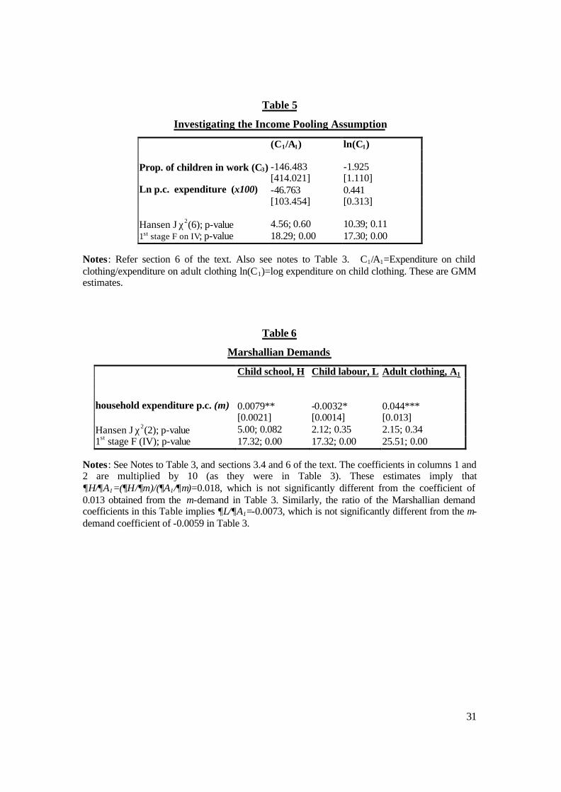
coefficient on this variable is positive. Results are in Table 5.24 The hypothesis of a

24 Total expenditure is instrumented with a cubic in income (as, for example in Blundell et al 1998). Additional instruments used to allow for the potential endogeneity of the child labour term are the community-level wage rates for children and adults, and indicators for the

19

positive coefficient is decisively rejected (by OLS, LIML and GMM estimates). The

coefficient on the child labour variable is insignificantly different from zero,

consistent with income pooling. As a further check on this, the m-demand for

schooling was estimated on the sample of households in which no child works, and

the coefficient ∂H/∂Aj was not significantly different from that obtained on the full

sample. Results are in column 1, Table 7.

Recall that the strategy of using income as an instrument for adult

consumption in the equation for child labour relies upon assuming separability of

adult and child labour. While this is quite standard in the literature, it is questionable

(see Bhalotra 2002). Table 7 shows estimates that condition on adult labour supply,

first total, and then separating adult males and females. The parameters of interest,

∂H/∂Aj and ∂L/∂Aj, are not significantly changed. Consistent with altruism, the

coefficient on adult labour is positive in the child labour equation, and negative in the

schooling equation. In other words, the data show that child labour is associated with

a cutting back of adult consumption and leisure (and conversely, in the case of

schooling). There is no significant difference in the coefficients on adult male and

female labour supply. In columns 2 & 3, parental labour is assumed exogenous, which

is common in many theoretical and empirical studies of child labour. In columns 4 &

5, it is instrumented with the education and age (and interactions thereof) of the

parents (these are conventional instruments; see, for e.g., Browning and Meghir

1991). The results are robust to this variation.

Although economists acknowledge that fertility is a choice variable, this is

commonly ignored in empirical work, and household size is typically treated as an

exogenous control variable. A justification of this is to argue that conditioning on size

produces a short run effect, which may usefully be compared with the corresponding

long run relation by omitting size (e.g. Deaton 1997: p. 221). Dropping size25

produces the results in column 6, Table 7, which show robustness of the key

coefficient to this change.

presence of primary, middle and secondary schools in the community. Tests on the instruments are reported in the Tables. 25 Household size is not the same as fertility. However, in rural households that contain non-nuclear families, adult membership of the household is likely to be correlated with choices over the quantity and quality of children. It is therefore cleaner to allow for the endogeneity of total household size.

20

Table 6 reports estimates of Marshallian demands for each of the child

outcomes (H, L) and adult clothing expenditure, A1 (refer section 2.4). The ratio of the

income effects from the Marshallian demands produces a point estimate that is larger

but not significantly different from the corresponding m-demand estimate of the key

parameter, ∂H/∂A1, or ∂L/∂A1 (see Notes to Table 6).

The square of expenditure on the reference good was included as an additional

regressor but in no case was it significant. This is backed by the Hansen-Sargan tests

(see footnote 26). I also investigated a specification in which all expenditures are in

logarithms (Table 7). The elasticities derived from these models are not significantly

different from unity (see Wald tests in Table 7), consistent with a Cobb-Douglas

specification. The pattern of coefficients in the logarithmic model is the same as in the

main results. As the dependent variables are proportions, I investigated robustness to

using the two-limit tobit estimator. As the results were similar, they are not shown.

Alternative equations using average hours in work and school instead of the

proportion of participating children in the household were also estimated, with

qualitatively similar results (results available on request).

5 Conclusions

This paper produces estimates of the contemporary sharing of household resources

between adult consumption and child schooling or, in an alternative specification,

child labour. It finds that increases in adult consumption are positively associated with

the proportion of children in the household who attend school, and negatively

associated with the proportion who are engaged in work. These results obtain in a

number of specifications of the model, including one in which adult labour supply is

held constant. The finding that increases in child labour are associated with decreases

in adult consumption allows us to reject the view prevalent in some previous research

(see section 1) that parents make child labour choices with a view to their personal

gain. These results are non-trivial, given previous rejections of altruism (see section

1). The paper also presents evidence that, as is commonly assumed, the earnings of

working children are pooled with other household income. There is some indication

that, at given living standards, households in which tobacco is consumed are more

likely to engage their children in labour. The results of this paper are relevant to the

vast body of research in which parental altruism is axiomatic. They are also relevant

21

to policy since, if altruism were weak, then policies that constrain the behaviour of

parents- like legislative interventions or conditionality in cash transfers- would gain

strength.

22

References Ahmad, A. & Morduch, J., 1993. "Identifying Sex Bias in the Allocation of Household Resources: Evidence from Linked Household Surveys from Bangladesh," Harvard Institute of Economic Research Working Papers 1636, Harvard - Institute of Economic Research. Altonji, Joseph (1986), Intertemporal substitution in labour supply: Evidence from micro data, Journal of Political Economy, 94(3), Part 2, June, pp. S176-215. Altonji, Joseph, Fumio Hayashi and Laurence Kotlikoff (1992), “Is the extended family altruistically linked? Direct tests using micro data”, American Economic Review, December, 1177-1198. Altonji, Joseph, Fumio Hayashi and Laurence Kotlikoff (1997) “Parental altruism and inter-vivos transfers: Theory and evidence”, Journal of Political Economy, Vol. 105 (6), 1121-66. Attanasio, O. and V. Lechene (2003). Tests of income pooling in household decisions, Review of Economic Dynamics, 5, 720-748. Attanasio, O. and T. MaCurdy (1997), Interactions in family labour supply and its implications for the impacts of EITC, mimeo, London: UCL. Baland, J. M. and J. Robinson (2000), “Is Child Labor Inefficient?”, Journal of Political Economy, August, 108(4), 663-79 Banerjee, Abhijit (2004), Educational policy and the economics of the family, Journal of Development Economics, Volume 74(1), June, pp. 3-32. Bangladesh Bureau of Statistics (1996), Report on National Sample Survey of Child Labour in Bangladesh, 1995-96, Dhaka: BBS. Barro, Robert J. (1974) “Are government bonds net wealth?”, Journal of Political Economy, 82, 1095-1117. Basu, Kaushik and Van, P.(1998), “The Economics of Child Labor”, American Economic Review, 88(3), June, 412-427. Becker, Gary (1981) “Altruism in the Family and Selfishness in the Market Place”, Economica, 48, February 1-15 Becker, G. S. (1991), A Treatise on the Family, Cambridge and London: Harvard University Press. Becker, G.S. (1999), “Bribe” third world parents to keep their kids in school, Business Week , November 22. Becker, G.S. and Murphy, K.M. (1988), “The Family and the State”, Journal of Law and Economics, 31(1), April, 1-18 Becker, G.S. and Tomes, (1986) “Human Capital and the Rise and Fall of Families”, Journal of Labor Economics, 4(3), Part 2: The Family and the Distribution of Economic Rewards, July, S1-S39.

23

Behrman, J. and J. Knowles (1999), “Household Income and Child Schooling in Vietnam”, The World Bank Economic Review, 13(2), May. Behrman, Jere (1997), Intrahousehold distribution and the family, in Mark Rosenzweig and Oded Stark (Eds.), Handbook of Population and Family Economics, Volume 1A, Amsterdam: Elsevier Science. Bhalotra, S. (2000) “Is Child Work Necessary?”, STICERD Discussion Paper 26, London School of Economics, September. Revised version: Working Paper, Department of Economics, University of Bristol, August 2003. Bhalotra, S. (2001), Parent altruism, Mimeograph, University of Bristol. Available at http://ideas.repec.org/p/ecj/ac2002/25.html and http://info.worldbank.org/etools/docs/voddocs/190/374/parent_altruism.pdf. Bhalotra, S. (2002) , “Investigating separability of parent and child labour”, Paper presented at the AEA Meetings, Washington DC, January 2003. Mimeograph, Department of Economics, University of Bristol. Bhalotra, S. (2003), Child labour in Africa and Asia, Background research paper commissioned for the Education For All Monitoring Report, Paris: UNESCO. Bhalotra, S. (2004), “Parent altruism, cash transfers and child poverty”, Paper presented at the AEA Meetings, Atlanta, January 2002. Mimeograph, Department of Economics, University of Bristol. Bhalotra, S. and Attfield, C (1998) “Intrahousehold resource allocation in rural Pakistan: A semiparametric analysis” Journal of Applied Econometrics, 13(5), September/October, 463-480 Bhalotra, S and Heady, C. (2004) “Child Farm Labor: The Wealth Paradox”, World Bank Economic Review, Volume 17, Number 2, January, pp.197-229. Bhalotra, S. and Z. Tzannatos (2003), Child labor: what have we learnt? Social Protection Discussion Paper No. 0317, Washington DC: The World Bank, September 2003. Bhatty, K. (1998), “Educational deprivation in India: A survey of field investigations”, Economic and Political Weekly, 33(27), 1731-40 and 33(28), 1858-69. Blow, Laura, Ian Walker and Yu Zhu (2004), Who benefits from child benefit?, Mimeograph, IFS and University of Warwick. Blundell, R, A.Duncan and K. Pendakur (1998), Semiparametric estimation and consumer demand, Journal of Applied Econometric s, 13, 435-461. Bommier, Antoine and Pierre-Andre Dubois (2003), "Rotten Parents and Child Labor," Journal of Political Economy, forthcoming. Bound, J, Jaeger, DA and Baker, RM (1995), “Problems with instrumental variables estimation when the correlation between the instruments and the endogenous explanatory variable is weak”, Journal of the American Statistical Association, 90(430), 443-450 Browning, Martin (1998), “Modelling Commodity Demands and Labour Supply with M-demands”, Mimeograph, Institute of Economics, University of Copenhagen.

24

Browning, M., Bourguignon, F., P.-A. Chiappori and V. Lechene (1994), Incomes and outcomes: A structural model of intrahousehold allocation, Journal of Political Economy, Vol. 102, pp. 1067-96. Browning, Martin and Pierre-Andre Chiappori (1998), Efficient intra-household allocations: A general characterization and empirical tests, Econometrica, Vol. 66(6), November, 1241-78. Browning, M. and C. Meghir (1991), “The Effects of Male and Female Labor Supply on Commodity Demands”, Econometrica, 59(4), July, 925-951. Burra, Neera (1995), Born to Work : Child Labour in India, Delhi: Oxford University Press. Cox, D. (1987), “Motives for Private Income Transfers”, Journal of Political Economy, 95, June, 508-546. Currie, Janet (1995), Welfare and the wellbeing of children, 59, in Fundamentals of Pure and Applied Economics, Harwood Academic Publishers. Davidson, R. and J. McKinnon (1993), Estimation and Inference in Econometrics, Oxford: Oxford University Press. Deaton, A. (1985), Demand Analysis in Zvi Griliches and M.D. Intriligator eds., Handbook of Econometrics, vol. 3, Amsterdam: North Holland. Deaton, Angus (1989), Looking for boy-girl discrimination in household expenditure data, World Bank Economic Review 3: 1-15. Dessy, S and Pallage, S (2001), “Child Labor and Coordination Failures” Journal of Development Economics 65(2), 469-476 Duflo, Esther (2003), Grandmothers and granddaughters: Old-age pension and intra-household allocation in South Africa, World Bank Economic Review, Volume 17(1), 1-25. Edmonds, Eric (2002), Reconsidering the labelling effect for child benefits: Evidence from a transition economy, Economics Letters, August, pp. 303-9. Edmonds, Eric (2004), Does illiquidity alter child labour and schooling decisions?: Evidence from household responses to anticipated cash transfers in South Africa, NBER Working Paper No. 10265, February. Cambridge MA: National Bureau of Economic Research. Ermisch, John (2003), An Economic Analysis Of The Family, Princeton: Princeton Uni. Press. Fitzsimons, Emla (2003), The effects of risk on education and child labour, IFS working paper W02/07, London: Institute of Fiscal Studies. Fyfe, Alec (1989) Child Labour, Cambridge: Polity Press. Gupta, Manash (2000), Wage determination of a child worker: A theoretical analysis, Review of Development Economics. Haveman, R. and B. Wolfe (1995), “The Determinants of Children’s Attainments: A Review of Methods and Findings”, Journal of Economic Literature, 33, 1829-1878.

25

Hayashi, F. (1995), “Is the Japanese Extended Family Altruistically Linked? A Test Based on Engel Curves”, Journal of Political Economy, 103(3), June, 661-674. Heckman, J. (1974), Effect of childcare programs on women’s work effort, Journal of Political Economy, 82(2), Part II, March-April, S136-S163. ILO (1996), Economically Active Populations: Estimates and Projections, 1950-2010, Geneva: International Labour Organisation.

Keen, Michael (1986), Zero expenditures and the estimation of Engel curves, Journal of Applied Econometrics, Vol. 1, No. 3, July, pp. 277-286. Khan, Ali (2001), “Child Stitchers in Sialkot’s Export based Soccer Ball Manufacturing Industry”, Mimeograph, Department of Anthropology, University of Cambridge. Kochar, Anjini (1999), Returns to education and educational investments: Empirical evidence from rural Pakistan, Mimeograph, Stanford University. Kochar, A. (2000), “Parental Benefits from Intergenerational Coresidence: Empirical Evidence from Rural Pakistan”, Journal of Political Economy, December, 108(6), 1184-1209 Kooreman, Peter (2000), The labelling effect of a child benefit system, The American Economic Review, Vol. 90(3), June, 571-583. Laitner, John (1997), Intergenerational transfers and interhousehold economic links, in Mark Rosenzweig and Oded Stark (Eds.), Handbook of Population and Family Economics, Volume 1A, Amsterdam: Elsevier Science. Lillard, Lee and Robert Willis (1997), “Motives for Intergenerational Transfers: Evidence from Malaysia.” Demography, 34(1):115-34. Little, R.J.A., and Rubin, D.B. (1987), Statistical Analysis with Missing Data, New York: John Wiley Lopez-Calva, L.F. and Miyamoto, K (2004) “Filial Obligations and Child Labor”, Review of Development Economics, 2004, 8(3), 489-504 Loury 1981 Intergenerational transfers and the distribution of earnings, Econometrica, Vol 49(4), July, 843-67. Lucas, R. and Stark, O. (1985) Motivations to remit: evidence from Botswana, Journal of Political Economy 93: 901-18. Maurin, E (2002), "The impact of parental income on early schooling transitions: a re-examination using data over three generations”, Journal of Public Economics, vol.85 (3), pp: 301-332. Mayer, S. (1997), What Money Can’t Buy: Family Income and Children’s Life Chances, Cambridge Mass: Harvard University Press. Meghir, C and Weber, G (1996), “Intertemporal Nonseparability or Borrowing Restrictions? A Disaggregate Analysis using a U.S. Consumption Panel”, Econometrica, 64(5), September, 1151-1181

26

Moehling, C (2003), She has suddenly become powerful: Youth employment and household decision making in the early twentieth century, Mimeograph, Economic Growth Centre, Yale University. Moreira, M (2002), Tests with Correct Size in the Simultaneous Equations Model, PhD Thesis, University of Berkeley, December. Available at http://post.economics.harvard.edu/marcelo/papers.html Moreira, M and Poi, B (2003) “Implementing Tests with Correct Size in the Simultaneous Equations Model”, The Stata Journal, 3(1), 57-70 Nardinelli, C. (1990), Child Labor and the Industrial Revolution, Bloomington: Indiana University Press. Nugent, J.B. (1985), “The Old-Age Security Motive for Fertility”, Population and Development Review, 11(1), March, 75-97. Pal, S. (2004), Do Children Act As Old Age Security in Rural India? Evidence from an Analysis of Elderly Living Arrangements', May. Mimeograph, Department of Economics, Cardiff University. Parish, W.L. and Willis, R.J. (1993), “Daughters, Education, and Family budgets Taiwan Experiences (in Education)”, The Journal of Human Resources, 28(4), Special Issue: Symposium on Investments in Women's Human Capital and Development, 863-898. Parsons, D. and C. Goldin (1989), “Parental Altruism and Self-Interest: Child Labor among Late Nineteenth Century American Families”, Economic Inquiry, 637-659. Ranjan, P. (2001), Credit constraints and the phenomenon of child labor, Journal of Development Economics, 64(1), March 2001. Ravallion, M., Wodon Q. (2000), “Does child labour displace schooling? Evidence on behavioural responses to an enrollment subsidy”, Economic Journal, 110 (462), March, C158-C175 Rogers, Carol Ann and Kenneth Swinnerton (2003), “Does child labour decrease when parental incomes rise?”, March, Working Paper available at http://www.georgetown.edu/faculty/rogersc/Papers/Altruism.pdf.

Rogers, Carol Ann and Kenneth Swinnerton (2004), Does child labour decrease when parental incomes rise?, Journal of Political Economy, August, 939-946.

Rosenzweig, M. and T.P. Schultz (1989), “Schooling, information and nonmarket productivity – contraceptive use and its effectiveness”, International Economic review, 30(2), May, 457-477 Shea, J.(2000), Does Parents’ Money Matter? Journal of Public Economics, 77(2), 155-84. Staiger, D and Stock, JH (1997) “Instrumental Variables Regression with Weak Instruments”, Econometrica 65(3), May, 557-586 Stock, JH and Watson, MW (2002), Introduction to Econometrics, Addison-Wesley. Wooldridge, J. M. (2002), Econometric Analysis of Cross Section and Panel Data , The MIT Press, Cambridge, Massachusetts.

27

Table 1

Descriptive Statistics

Mean across households

Standard deviation

Expenditure elasticity

Budget shares: Adult clothing & footwear (A1) 0.043 0.035 0.76 Tea & coffee (A2) 0.018 0.014 0.60 Tobacco (A3) 0.020 0.028 0.43 Adult expend (A4=A1+ A2+ A3) 0.082 0.051 0.68 Child clothing & footwear (C) 0.029 0.024 0.79 Food 0.537 0.165 0.74 Education 0.035 0.053 0.96 Health 0.103 0.137 1.13 Ceremonies 0.031 0.065 1.20 Prop. children in household in work 0.324 0.422 -0.27

Prop. children in household in school 0.518 0.445 0.25

Prop. households with at least 1 child in work 0.410 (0.492) -0.11* Prop. households with at least 1 child in school 0.628 (0.483) 0.11* Expenditure in Rupees: Total expenditure per capita (m) 500.72 492.84 Adult clothing & footwear (A1) 43.56 45.98 Tea & coffee (A2) 17.65 15.77 Tobacco (A3) 19.35 29.95 Adult expend: aggregate of above three items (A4) 80.55 65.93 Child clothing & footwear (C) 26.71 27.00

Notes: N=1340 households. The figures in columns 1-2 are means and standard deviations of shares of total household expenditure. The elasticities in column 3 are obtained as θ from simple regressions of the form lnXk=θlnX+u, where Xk is normalised expenditure for each item in column 1 and X is total expenditure per capita. For the adult goods, the natural normalisation of expenditure is per adult. For child clothing and education, it is per child. For food, health and ceremonies, it is per household member. A * indicates marginal effects of the log of total expenditure per capita obtained from a probit with dependent variable defined as unity if at least one child in the household works (or attends school). Every reported elasticity is statistically significant. A substantial fraction of households report zero spending on tobacco, ceremonies, health and education. In these cases the expenditure elasticity is computed for the sub-sample of households that record positive expenditure. The means of rupee expenditure are used to calculate elasticities using the estimated coefficients in Table 3.

28

Table 2

Is Adult Consumption Sensitive to whether Children are in Work or School? Tests of differences in means

(1) (2) (3) (4) (5) Adult Expenditure (per adult): Difference:

E0 - E1 t-statistic p<t:

HA: diff<0 p>|t| HA: diff≠0

p>t HA: diff>0

Panel 1: [Child labour, L] Adult clothing and footwear (A1) 4.89 1.92 0.97 0.06* 0.03* Tea and coffee (A2) -1.34 -1.53 0.06* 0.13 0.94 Tobacco (A3) -2.95 -1.78 0.04* 0.08* 0.96 “Adult goods”: aggregate of the above (A 4) -0.62 -0.08 0.47 0.94 0.53 Tobacco: sub-sample with exp>0 (A3) -0.91 -0.43 0.34 0.67 0.67 Panel 2: [Child schooling, H] Adult clothing and footwear (A1) -5.18 -2.00 0.02* 0.05* 0.98 Tea and coffee (A2) 0.34 0.38 0.65 0.71 0.35 Tobacco (A3) 0.32 0.19 0.58 0.85 0.42 “Adult goods”: aggregate of the above (A 4) -18.62 -2.31 0.01* 0.02* 0.99 Tobacco: sub-sample with exp>0 (A3) 0.02 0.01 0.50 0.99 0.50 Notes: The sample is divided into the 791 (41%) households in which at least one child aged 10-14 is reported as working in the reference week (group 1), and the remaining 549 (59%) households with no child labour (group 0). Column 1 reports the difference in adult expenditure between these two samples. A negative difference indicates that more is spent on adult consumption in the average household when children work- contrary to what is expected under altruism. Column 2 presents the t-statistic associated with this difference. The null hypothesis is that the difference is zero. The p-values in columns 3-5 indicate whether the difference is statistically significant for the 1-tailed and 2-tailed tests defined in terms of the alternative hypotheses, HA. The analysis is repeated in Panel 2 of the Table, with sub-samples defined as the 842 (63%) households in which at least one child attended school in the reference week, and the remaining 498 (37%) households. If schooling is a good, while child labour is a bad, the signs are now in reverse. A negative difference indicates that more is spent on adult consumption in the average household when children attend school- and this is consistent with altruism. All expenditures are in Rupees per adult to allow for differences across households in the number of adults. Since 30% of households exhibit zero expenditure on tobacco, t-tests are presented separately for the sub-sample of households that report positive tobacco expenditure.

29

Table 3

Child Schooling & Child Labour

GMM & LIML Estimates of M-Demands

SCHOOLING (H) Adult clothing Tea & Coffee Tobacco (smokers)

Adult goods

Panel 1: GMM Estimates (A1) (A2) (A3) (A4) Adult expenditure (x10) 0.132** 0.606** 0.146* 0.084**

[0.034] [0.221] [0.064] [0.021] Hansen’s J χ2; p-value 3.60; 0.17 0.90; 0.64 1.61; 0.45 2.67; 0.26 1st stage F on IV; p-value 8.65; 0.00 4.59; 0.01 6.42; 0.00 11.94; 0.00 Panel 2: LIML Estimates Adult expenditure (x10) 0.154** 0.685** 0.171** 0.095** [0.046] [0.259]] [0.060] [0.026] LR test; 95% critical value 35.99; 5.41 40.21; 5.21 19.30; 4.56 37.03; 5.05 Wald test; 95% critical value 12.50; 3.57 7.48; 2.82 8.24; 2.92 14.52; 3.53 Panel 3: OLS Estimates Adult expenditure (x100) 0.096** 0.043 0.057 0.046* [0.038] [0.081] [0.051] [0.022] R-square 0.19 0.16 0.16 0.16 CHILD LABOUR (L) Panel 1: GMM Estimates

Adult expenditure (x10) -0.059** -0.267* -0.055+ -0.038**

[0.021] [0.131] [0.031] [0.013] Hansen J χ2; p-value 1.65; 0.44 1.49; 0.48 1.04; 0.59 1.32; 0.52 1st stage F on IV; p-value 8.65; 0.00 4.59; 0.01 6.42; 0.00 11.94; 0.00 Panel 2: LIML Estimates Adult expenditure (x10) -0.060** -0.291** -0.076+ -0.039** [0.026] [0.149] [0.041] [0.016] LR test; 95% critical value 7.13; 4.68 7.36; 5.20 4.23; 4.56 7.25; 4.37 Wald test; 95% critical value 5.31; 3.36 3.77; 2.82 3.38; 2.90 5.57; 3.44 Panel 3: OLS Estimates Adult expenditure (x10) -0.067** 0.035 -0.064 -0.029 [0.024] [0.081] [0.050] [0.018] R-square 0.12 0.11 0.12 0.12 N 1327 1327 927 1327

Notes: The dependent variable is the proportion of children 10-14 years in the household that attend school and work respectively. See section 4.3 for details of the estimators and tests. Robust standard errors in brackets. + significant at 10%; * significant at 5%; ** significant at 1%.

30

Table 4 Do Children Get Less in Smoking Households (A3>0)?

Tests of conditional mean differences

Schooling Child labour Regression estimates tobacco expenditure 0.252** -0.110* [0.111] [0.050] 1(tobacco>0) -0.744** 0.392* [0.300] [0.153] Hansen J χ2; p-value 2.69; 0.26 1.05; 0.59 1st stage F on IV; p-value 3.31; 0.04 3.31; 0.04 T-tests Difference: C0 - C1 0.22 -0.31 t-statistic 5.96 -21.0 p<t: HA : diff<0 1.00 0.00 p>|t|: HA: diff≠0 0.00 0.00 p>t: HA : diff>0 0.00 1.00 % change -32.1 300.0

Notes: the reference good is tobacco expenditure. This is similar to column 3 of Table 3 except that now all households are used and a dummy variable (DS) is defined which equals unity for the 927 (70%) households that report positive expenditures on tobacco and zero for the remaining 400 (30%) households. So C = γ3A3 + γSDS + θZ + e. Row 2 shows that γS<0. The predicted level of C in a smoking household (DS=1) is C1= γ3A3

+ γS + θZ and the predicted C in a non-smoking household (DS=0) is C0= θZ. The mean difference is (C0 - C1), reported with its t-statistic. The null hypothesis is that the difference is zero. The p-values indicate whether the difference is statistically significant for the 1-tailed and 2-tailed tests defined in terms of the alternative hypotheses, HA. The final row indicates the size of the difference. This is defined as (C0 - C1)/ C0, expressed in percentage terms.

31

Table 5

Investigating the Income Pooling Assumption

(C1/A1) ln(C1) Prop. of children in work (C3) -146.483 -1.925 [414.021] [1.110] Ln p.c. expenditure (x100) -46.763 0.441

[103.454] [0.313] Hansen J χ2(6); p-value 4.56; 0.60 10.39; 0.11 1st stage F on IV; p-value 18.29; 0.00 17.30; 0.00

Notes: Refer section 6 of the text. Also see notes to Table 3. C1/A1=Expenditure on child clothing/expenditure on adult clothing ln(C1)=log expenditure on child clothing. These are GMM estimates.

Table 6

Marshallian Demands

Child school, H Child labour, L Adult clothing, A1

household expenditure p.c. (m) 0.0079** -0.0032* 0.044***

[0.0021] [0.0014] [0.013] Hansen J χ2(2); p-value 5.00; 0.082 2.12; 0.35 2.15; 0.34 1st stage F (IV); p-value 17.32; 0.00 17.32; 0.00 25.51; 0.00

Notes: See Notes to Table 3, and sections 3.4 and 6 of the text. The coefficients in columns 1 and 2 are multiplied by 10 (as they were in Table 3). These estimates imply that ∂H/∂A1=(∂H/∂m)/(∂A1/∂m)=0.018, which is not significantly different from the coefficient of 0.013 obtained from the m-demand in Table 3. Similarly, the ratio of the Marshallian demand coefficients in this Table implies ∂L/∂A1=-0.0073, which is not significantly different from the m-demand coefficient of -0.0059 in Table 3.

32

Table 7

Alternative Specifications

Sub-sample with no child labour

Control for adult labour (exog)

Control for male and female adult labour (exog)

Control for adult labour (IV)

Control for male and female adult labour (IV)

Drop household size

Expenditure in logs

Dependent variable: school (H) Adult clothing expenditure (A1) 0.108** 0.148** 0.144** 0.154** 0.131** 0.118** 0.486**

[0.037] [0.044] [0.043] [0.031] [0.034] [0.039] [0.140] Adult labour -0.218** -0.180

[0.079] [0.333] Adult female labour -0.118* -0.498

[0.048] [0.393] Adult male labour -0.147* 0.254

[0.061] [0.359] Hansen J χ2; p-value 1.49; 0.47 0.29; 0.87 0.28; 0.87 8.23; 0.31 7.98; 0.24 3.28; 0.91 6.14; 0.06 1st stage F on IV; p-value 5.12; 0.01 7.63; 0.00 7.62; 0.00 6.85; 0.00 6.47; 0.00 4.76; 0.00 7.14; 0.00 Wald test elasticity(γ)=1: χ2(1); p -value 0.05; 0.82 Dependent variable: child labour (L) Adult clothing expenditure (A1) -0.057* -0.053* -0.065** -0.056** -0.074** -0.296**

[0.026] [0.022] [0.017] [0.021] [0.028] [0.091] Adult labour 0.439** 0.415*

[0.048] [0.192] Adult female labour 0.282** 0.371

[0.026] [0.301] Adult male labour 0.101* 0.103

[0.039] [0.235] Hansen J χ2; p-value 0.19; 0.91 0.04; 0.98 11.10; 0.13 11.04; 0.09 4.62; 0.10 6.02; 0.05 1st stage F on IV; p-value 7.63; 0.00 7.62; 0.00 6.85; 0.00 6.47; 0.00 4.76; 0.00 7.14; 0.00 Wald test elasticity(γ)=1: χ2(1); p -value 0.10; 0.76 N 780 1324 1312 1324 1312 1318

Notes: See Notes to Table 3, which presents the benchmark model. All estimates are GMM. The C-statistic that tests the additional restrictions implied by the instruments used for adult labour is 7.99 (p -value=0.24) in the schooling equation and 11.1 (p=0.11) in the child labour equation, which confirms that the instruments are valid. The estimated coefficients in the last column correspond to ∂H (or ∂L)/ ∂logA and so the elasticities, ∂logH/ ∂logA (=0.94) and ∂logL/ ∂logA (=0.91), can be derived by dividing these coefficients by the mean of H (0.518) or L (0.324).The Wald tests are of the null that the elasticity is 1 (–1 in the case of child labour).

33

Figure 1: Conditional Likelihood Ratio Test Statistics and Critical Values Adjusted for Weak Instruments

Notes: See Section 4.3 of the text. Beta is the (scaled) coefficient on the adult expenditure. The asymptotic critical value (CV) is the flat line (lr), the adjusted CV is the jagged line (lrcrit) and the confidence region is the region of the graph where the observed statistic (the smooth curve) lies below its critical value.

010

2030

40T

est s

tatis

tic a

nd c

ritic

al v

alue

0 1 2 3 4beta

lr lrcritA

sym

ptot

ic C

V a

lso

show

nConfidence Region

010

2030

4050

Tes

t sta

tistic

and

crit

ical

val

ue

-5 0 5 10 15beta

lr lrcrit

Asy

mpt

otic

CV

als

o sh

ownConfidence Region

010

2030

Tes

t sta

tistic

and

crit

ical

val

ue

-1 0 1 2 3 4beta

lr lrcrit

Asy

mpt

otic

CV

als

o sh

ownConfidence Region

010

2030

40T

est s

tatis

tic a

nd c

ritic

al v

alue

0 .5 1 1.5 2beta

lr lrcrit

Asy

mpt

otic

CV

als

o sh

ownConfidence Region

1. Adult clothing, 2. Tea & coffee, 3. Tobacco, 4. Aggregate of 1-3. Details in text

beta is coefficient on Aj*100

Moreira's LR StatisticSchool Attendance

05

1015

20T

est s

tatis

tic a

nd c

ritic

al v

alue

-1.5 -1 -.5 0 .5beta

lr lrcrit

Asy

mpt

otic

CV

als

o sh

ownConfidence Region

05

1015

Tes

t sta

tistic

and

crit

ical

val

ue

-8 -6 -4 -2 0 2beta

lr lrcrit

Asy

mpt

otic

CV

als

o sh

ownConfidence Region

05

1015

Tes

t sta

tistic

and

crit

ical

val

ue

-3 -2 -1 0 1beta

lr lrcrit

Asy

mpt

otic

CV

als

o sh

ownConfidence Region

05

1015

20T

est s

tatis

tic a

nd c

ritic

al v

alue

-1 -.5 0 .5beta

lr lrcrit

Asy

mpt

otic

CV

als

o sh

ownConfidence Region

1. Adult clothing, 2. Tea & coffee, 3. Tobacco, 4. Aggregate of 1-3. Details in text

beta is coefficient on Aj*100

Moreira's LR StatisticChild Labour