EI UGEG·V'Gt:"'l 1 .... ·- '0 "6 I~ r\h 1.:..·12, h·i.:. 1~0

Nr. 81 Mitteilungen der Versuchsanstalt fOr Wasserbau, Hydrologie und Glaziologie

an der Eidgenossischen Technischen Hochschule Zurich Herausgegeben von Prof. Dr. D. Vischer

DYNAMICS OF

POWDER-SNOW AVALANCHES

Thomas Scheiwiller

Zurich, 1986

- 3 -

- 4 -

PREFACE

The repeated casual ties that occur every year in

Switzerland in connection with snow avalanches make it

mandatory that any government of a country situated in a

mountaneous area supports related research units so that

hazards and destructions caused by avalanches can be mi­

nimized. Avalanche motion can, however, not be prevented

under all circumstances. Hence, the understanding of the

physical mechanisms that underly their motion becomes

important as avalanche zoning depends on these. It ap­

pears obvious that field experiments are not suitable

for this task. Laboratory experiments do provide the only

other alternative to study such processes and to test

theoretical models with experimental findings.

This report is an account on exactly this latter aspect.

A theory which describes avalanches as a turbulent two

phase flow is deduced, an experimental set- up for labo­

ratory avalanches is constructed and a measuring tech­

nique to obtain velocities and snow particle concentra­

tions is designed which allows a suitable test of the

theory. With the results of this report it has now become

possible to study certain avalanche phenomena by physi­

cal models, a tool that may not replace other studies

but certainly will facilitate further research.

The work was performed with support from the Swiss

National Science Foundation and the Swiss Institute for

Snow and Avalanche Research.

K. Hutter

- 5 -

Contents

AB STRACT

ZUSMI}!ENFASSUNG

RESUME

1. Introduction

2. Theory of powder-snow avalanches 2.1 Preliminar ies

2.2 The continuum approximation

2.3 Governing equations

2 . 3 .1 Two- phase flow

2 . 3.2 Averaged equations for turbulent flow

2 . 3 . 3 Turbulence model

2 . 3 . 4 Inte rphase friction

2.4 Application to plane two - phase shear flow down an inclined chute

2.4 .1 Balance equations

2 . 4 . 2 Boundary conditions

2 . 4 . 3 Compl ete mathematical formu l ation

page

7

8

9

ll

18

18

20

22

22

24

25

26

29

29

31

35

2.5 The steady-state p robl em and its significance 37

2.6 Kantorovich-technique 37

2.6 .1 Basic idea

2 . 6.2 Kantorovich-transformed system of equations

2.7 The finite difference technique

3. Laboratory simulation of powder-snow avalanches 3.1 Similitude and experimental set-up

3 .2 Measurement of particle ve locities by an ultrasonic Doppler technique

3.3 Measurement of the particle number density

3.4 Summary of experimental results

3.5 Numerica l calculations

37

39

50

52

52

58

64

68

73

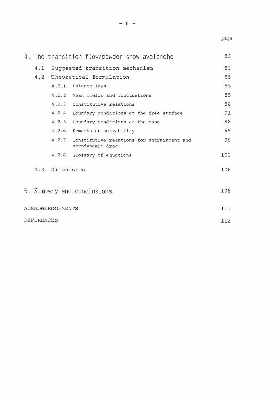
- 6 -

4. The transition flow/powder snow avalanche 4 .1 Suggested transition mechanism

4.2 Theoretical formulation

4.2.1 Balance laws

4.2.2 Mean fields and fluctuations

4 . 2.3 Constitutive relations

4.2.4 Boundary conditions at the free surface

4. 2 . 5 Boundary conditions at the base

4.2 . 6 Remarks on solvability

4 . 2 . 7 Constitutive re lations for entrainment and aerodynamic drag

4. 2 . 8 Glossary of equations

4.3 Discussion

5. Summary and conclusions

ACKNOWLEDGEMENTS

REFERENCES

page

83

83

85

85

85

88

91

98

99

99

102

106

108

111

112

- 7 -

ABSTRACT

A continuum theory for the dynamics of powder snow

avalanches is developed. They are treated as free sur­

face two - phase flows of snow particles and a ir, coup­

led by momentum transfer. Closure of the equat ions is

achieved by a k- E-model for the turbulence and by a

linear relationship between interphase momentum trans­

fer and the relative velocity of the phases. Numerical

so lutions obtained by means of the Kantorovich tech­

n ique are presented for steady plane flow. They are

compared with measurements from the small-scale labo­

ratory simu l ation of powder snow avalanches as turbu­

lent mix tures of polystyrene par ticles and water. Me ­

thods of measuring particle phase velocity profiles

and partic l e phase volume fraction profiles in steady

chute f l ow are presented.

A theoretical model for the transition from the

flow avalanche regime to the powder snow avalanche

regime is out lined. This transition may be treated as

an instability induced by the boundary condition at

the free surface: In a critical flow state, the en­

tra inment of ambient air is greatly enhanced .

- 8 -

ZUSAMMENFASSUNG

Ein kontinuumsmechanisches Modell flir die Dynamik

von Staublawinen wird entwickelt. Diese werden behan­

delt als Zweiphasenstromung mit freier Oberflache, be­

stehend aus Schneepartikeln und Luft, welche durch Im­

pulsaustausch gekoppelt sind. Das System von Gleichun­

gen wird geschlossen mit einem k-E-Modell flir die Tur­

bulenz und einer linearen Abhangigkeit des Impulsaus­

tausches von der Relativgeschwindigkeit der beiden Pha­

sen . Numerische Losungen flir stationare ebene Stromung,

welche mit Hilfe der Kantorovich-Technik erhal ten wur­

den, werden verglichen mit Messungen aus der kleinska­

ligen Laborsimulation von Staublawinen als turbulentes

Gemisch von Po l yesterharzpartikeln und Wasser . Messme­

thoden flir Geschwindigkeits- und Konzentrationsprofile

der Partikelphase werden vor gestel l t.

Ein theoret i sches l·lodell flir den Ubergang vom Fliess­

lawinen-Zustand in den Staublawinen- Zustand wird dar­

gelegt. Dieser Uebergang kann als durch die Randbedin­

gung an der freien Oberf l ache induzierte Instabili­

tat behandelt werden: In einem kritischen Stromungszu­

stand wachst die Menge der eingemischten Umgebungsluft

stark an.

- 9 -

RESUME

Un modEHe de la dynamique des avalanches de neige

poudreuse est developpe en mecanique des milieux conti­

nus. Ces avalanches sont traitees comme des ecoulements

A surface libre de deux phases, particules de neige et

air, couplees par transfert de la quantite de mouvement.

La fermeture du systeme d'equations est assuree par un

modele k- £ pour la turbulence et par une relation line­

aire entre le transfert de la quantite de mouvement et

l a vitesse relative des deux phases . La technique de

Kantorovich permet d' obtenir des solutions numeriques

pour un ecoulement p l an stationnaire . Ces solutions sont

comparees avec les mesures effectuees a petite echelle

en laboratoire sur la simulation d' avalanches poudreuses

par des melanges turbulents de particules de polysty­

rene et d' eau . Les methodes de me sure des prof ils de

vitesse et de concentration des particules sont de ­

crites.

Un modele theorique de la transi tion du regime d'ava­

lanche coulante au regime d ' avalanche poudreuse est ex­

pose . Cette transition peut etre consideree comme une

instabilite induite par la cond i tion limite sur la sur­

face libre: dans un etat d'ecoulement critique , l a quan­

tite d'air entrainee s ' accroit fortement.

- 11 -

1. Introduction

Avalanches belong to the kind of natural phenomena to which

the population in alpine regions is exposed during wintertime

and spring time. The research in ava lanche prevention and the

study of their dynamics are a duty of most of the mountaineous

nations . Avalanche hazard is not an invention of our century.

There exist many historical reports on snow avalanches. Among

the first is that of the ancient Greek geographer S:tlr.abon (63 b.C.

to 23 a.C.). He writes

" ... ice avalanches which often carry away with them whole tourist parties and throw them into the abyss. For numerous are the layers lying one above the other. The snow develops layer by layer to ice and the uppermost detaches from time to time before it has been molten by the sun."

Although Strabon writes "ice avalanches ", he certainly means

snow avalanches, because the former are not frequent .

U.v.i.116 , a roman contemporary of Strabon, mentions avalanches

in his description of Hannibal' s traverse of the Alps (218 b.C.)

"The snow cover was caused to glide down by the weight of man and an imals. "

The bishop I.6odoi!M o6 Se.villa (570-636 a.C.) is the first to

define "lavina" - latin for "ava lanche"- in his encyclopedia

as ''lavina, lapsum interferens: lavina eo, quod ambulantibus lapsum

inferat dicta per derivationem e la­bes ".

[" avalanche, causing tumble: ava l anche because it leads wanderers] to tumble, derived from "labes 11

(= tumble, fall) " ,

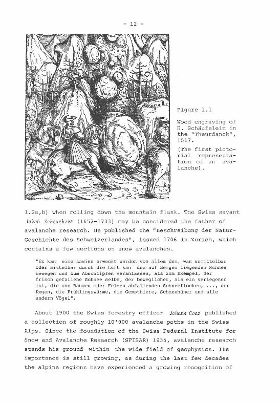
The first pictorial representation of an ava lanche (known

to date) appeared 1517 in the biography named "The.uJtdanc./z" of

the emperor Max.-<.milian. It is a wood engraving by H. Schaufe-

lein (see Figure 1.1). Up to the beginning of the twentieth

century, people imagined snow avalanches as large snow balls

which increase by accretion of the underlying snow (see Figure

- 12 -

Figure 1.1

Wood e ngrav ing of H. Schaufelein in the "Theurdanck", 1517.

(The first picto­rial representa­tion of an ava­lanche) .

1.2a,b) when rolling down the mountain flank . The Swiss savant

Jakob Scheuchz~ (1652-1733) may be considered the father of

avalanche research. He published the "Beschreibung der Natur­

Geschichte des Schweizerlandes", issued 1706 in Zurich, which

contains a few sections on snow avalanches.

"Es kan eine Lawine erweckt werden von allern dern, was unrnittelbar oder rnittelbar durch die Luft kan den auf Bergen liegenden Schnee bewegen und zurn Abschlipfen veranlassen, als zurn Exernpel, der frisch gefallene Schnee selbs, der beweglicher, als ein verlegener ist, die von Baurnen oder Felsen abfallenden Schneeflocken, der Regen, die Frlihl i ngswarrne, die Gernsthiere, Schneehliner und alle andern Vi:igel" .

About 1900 the Swiss forestry officer Johann Coaz published

a collection of roughly 10'000 avalanche paths in the Swiss

Alps . Since the foundation of the Swiss Federal Institute for

Snow and Ava lanche Research (SFISAR) 1935, avalanche research

stands his ground within the wide field of geophysics. Its

importance is still growing, as during the last few decades

the alpine regions have experienced a growing recognition of

a)

b)

- 13 -

Figur 1.2

Historical illustrations of snow avalanches (18th, 19th century) .

their economical and recreatio­

nal significance. Correspond­

ingly, ways of connection and

protectional measures of their

resources have grown and called,

among other things, for an ef ­

f icient avalanche protection.

In this regard, the optimal

design of protecting facilities

presumes knowledge about the

avalanche break-off, its motion

on the track and its behaviour

in the runout zone. Because

supporting structures in the

starting zone are expensive,

efforts are being chief l y fo-

- 14 -

cussed upon direct protection of endangered ob j ects such as

highways and indi vidual houses (see Perla and Martinelli, 1978).

The present avalanche knowledge suffers from an incomplete

understanding of this gravity driven flow phenomenon, probably

to a large extent because a thorough theoretical treatment

is still lacking. Despite the fact that there exist several

continuum mechanical attempts (Voellmy, 1955; Salm, 1966),

each of them deals only with a particular aspect of the ava­

lanche behaviour, be it the fracture of. the snow cover, the

motion of the snow on the avalanche track, or the decelerating

flow and the deposition processes in the runout zone (see Fi­

gure 1. 3).

starting zone

Figure 1.3

Illustrating starting zone, ava lanche track and run-out zone.

avalanche track

Avalanche research also lacks the collection of f i eld data

for velocities and densities of avalanches in motion. It is

only recently that a program of field measurements regarding

flow avalanches has been undertaken (Gubler, 1981; Gubler and

Hiller, 1984). In this regard, it should be mentioned that

snow avalanches may crudely be classified into t wo types (see

Figure l.4a,b) I namely olow avalanc.heo and powdVt ~now avalanc.heo.

The characterist ic features of each of these types are listed

in Table l.l. Most avalanches do not belong to one of these

limiting cases, but are rather a mixture of the two (see Fi-

I

- 15 --- - -

typi ea 1 velocity

flow hei ght

density

effect of topo9 t·a phy

related flo~1

phenornena

Table l .l

flow avalanche powder snow avalanche

30 --- 60 m s-1 :::::: lOO m s-1

:5 5 --- 10 m :::::: lOO m

:::: 11)0 --- 300 kg m-3 :::::: 5 kg m-3

avalanche is channeled none, following the by small valleys steepest descent

bed roughness important bed roughness unimportant

grain flow turbidity currents

Characteristic features of the two limiting cases of ava lanche.

I

gure l.4 c) . For powder snow avalanche s there e x ist e ven fewer

data, the only known parameters are the front ve locity and the

flow height. As l ong as the formation of powder snow avalanches

(i.e. the transition from the flow ava lanche to the powder snow

avalanche) is not fu lly understood (for a first theoretical

attempt see Chapter 4), no fie ld campaign concerning powder

snow avalanches is like ly to be successful, because no artifi­

cial release will g uarantee the format ion of a powder snow

avalanche. This dilemma l ed to the idea of a small scale labo­

ratory simulation of powder snow ava l anches (Davies, 1979).

This might appear superfluous, for theoretical and e xperimental

work on gravity-driven currents is well developed (Simpson,

1 982). However, within the common density current concepts, to

which all these works are restricted, sedimentation is not in­

corporated. But exactly the sedimentation processes on the

track and the snow deposition in the runout zone are crucial

processes. The only way of taking account of possible separa­

tion is a two-phase concept, which needs to b e studied, both

theoretically (Scheiwiller & Hutter, 1982) and exper imenta lly.

Clearly, it is doubtful whether or not the formation of powder

snow avalanches might ever be accessible by a laboratory simu­

lation and the present contribution deals neither with the

formation nor with the runout of powder snow ava lanches. But

it attempts to shed light on the characteristics of the ava-

- 1 6 -

a)

b)

Figure 1.4

Two limi ting cases of avalanches:

a) flow avalanche

b) powder snow avalanche

c) a mixed type (see next page)

- 17 -

C)

lanche motion along the track. This is done by laboratory si­

mulation and mathematical modeling in the following two chap­

ters (chapter 2 and chapter 3). Numerical results and experi­

mental data are restricted to the steady body of powder-snow

avalanches, however, and the transient head is not treated

(see Figure 1.5).

Figure l. 5

Illustrating the distinction between transient head and steady body.

Finally, chapter 4 is a first theoretical attempt to model

the transition from the flow avalanche regime to the powder

snow avalanche regime.

- 18 -

2. Theory of powder-snow avalanches

2.1 Preliminaries

In this section a series of requirements are given which a

mathematical mode l for powder snow avalanches must sat i fy. We

disregard the generation and formation of avalanches and re­

strict considerations to the evolution of pressure, velocity

and density f ields, once the powder snow ava lanche has fully

developed. Our particular interest is in profiles of these

field variabl es, that is the ir variations with the coordinate z

perpendicular ("cross stream") to the main ("downslope") flow

direction x (Figure 2.1). Information about these profiles is

indispensable for the estimation of the distribution of the

dynamical pressure upon buildings (houses , walls , rods, pylons

etc.) situated in the avalanche track o~ runout.

The theory thus must be two-dimensional at least. In s~neral

the avalanche process is three-dimensional, but we shall con­

sider plane flow in the xz -plane (Figure 2.1) only, because a

three-dimensional theory is rather involved. This restriction

is not serious, however, because a two-dimensional theory can

main

X

typical

velocity

typical

density

Figure 2.1

Definition of the xz- coordi­nate system and typical velo­city and density profiles.

- 19 -

be given a rational fundament by averaging the full three-di­

mensional equations in the third coordinate direction y.

Secondly, we demand that the model is able to describe the

deposition of the snow. This implies a t wo-phase theory. As a

matter of fact the "density-current concept" does not allow to

account for deposition*). We treat the snow phase as an assem­

blage of hard identical spheres, and neglect processes like

disintegration and coagulation of snow grains, heat and mass

transfer between snow particles and the ambient air (atmosphe­

re) and the rotation of snow particles. The energy balance is

therefore redundant,and we can restrict consideration to mass

and momentum balances only. Conservation of angular momenta

leads, in the absence of production terms, to the symmetry of

the stress tensors.

We assume the ambient air to b e incompressible. This appro­

ximation is valid, as long as the velocities (of snow and air)

are well below the speed of sound. The only possible interac­

tion left between snow and air is momentum transfer caused by

friction.

snow grains.

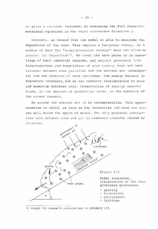
Figure 2.2

Model avalanche. Illustration of the four governing processes:

- gravity - tu.rbulence - entrainment - friction

*) Ex cept for Savage's calculations in EUROMECH 172.

- 20 -

Thus the "model avalanche" is a gravity driven turbulent

mixture of hard identical spheres and an incompressible Newto­

nian f luid. A mathematical treatment of the four bas ic proces­

ses (Figure 2.2) : gravity, turbulence, interphase friction and

entrainment of ambient air at the surface (see section 2.4.2)

wil l be worked out in the following sections.

2.2 The continuum approximation

The basic assumption in this theory is to treat the mixture

of particles and a fluid as two interpenetrating continua. We

have to show that this approximation is applicable in the flow

regime we are dealing with. (An alternative way of describing

a mixture would be to solve the equations of motion for every

partic le, for example).

In the absence of shear motion, body forces and chemical re­

actions the conservation of momentum of a suspension of one

species of solid particles can be expressed in one dimension

by Soo (1967)

d dtF

where

duF +

dup ap PF dtF Pp dtp ax'

a d a - + UF ax ' dtp at + Up at

UF fluid phase velocity , up particle phase velocity , PF fluid phase density, Pp particle phase density.

(2 .1) a

ax

Equation (2.1) treats the particle phase as a true continuum;

it implies that a cloud of particles can transfer momentum to

the fluid (in a turbulent motion : to the me.an flow of the fluid).

In a powder snow avalanche the snow particles do indeed drive

the air. The continuum approximation is in this case automati­

cally justified. It is obvious, however , that there exists a

lower limit for the particle phase density in the continuum

approximation. Below this critical density (or equivalently the

critical volume fraction) the particles cannot transfer momen­

tum to the mean fluid flow any longer, the corresponding energy

- 21 -

be ing d iss ipated in their wakes (see Figure 2 .3). We try to

quantify thi s critical vo lume fraction and proceed like Soo

did (Soo , 1967). Assume l a minar boundary layers around the so­

lid part i c l es (that is Rep = ( ap · I Vrell) /va ir $ 0 (1 )) ; Rep is called

the J.lCt"-'ttc.l'.e. Reynotd~ nwnbe.l[, whe r e ap is the radius of the parti­

cle and vre l the relat i ve velocity between particle and air .

Soo argues that the boundary layers of ad j acent particles must

overlap to have any effect of momentum transfer . In the case

dense suspensi on

l ean suspension

uF_ uP _____ _

uF_ uP _ ____ __

Fig ure 2.3

a) Dense c loud of solid particl es : negligible dissipation in wakes.

(from Soo , 1967, p . 261)

b) Lean sus pens i on: diss i pation in wakes without inc rease of mean kinetic energy on the intersti ­tial flu i d.

of a powder snow a va lanche such a criter i on under the above

mentioned assumpt ion leads to unrealistically high densities,

however . Thus we are forced to drop the assumpt i on of l ow par­

tic l e Reynolds number Rep (see sections 2.3.3). If the particle

Reyno lds number is sufficiently high*! (Vre l = 1 ms- 1 corresponds

to Rep = 0 (10 2) if ap = 0 (lo- 3 m)) t he particles interact through

their wakes. In a turbulent flow regime the minimum vo lume

fraction thus decreases.

Although the continuum approxima tion is a rather serious

o ne, it is intrinsically satisfied for fully developed powder

snow avalanches .

*) This is a reasonable estimation s ince the slip velocity must at least be of the same order of magnit ude as the free fall velocity of the snow particles in air (lvhich is 4 m s - 1 for a= lo-3 m, see Melior, 1977) to

keep the snow in suspension.

- 22 -

2 . 3 Governing equations

2.3.1 Two-phase flow

In a mixture each phase can be described as a continuum,

governed by the partial differential equations of continuum

mechanics ext~nded by terms taking into account transfer pro­

cesses (mass, momentum, heat transfer) among the phases. In

the model avalanche (see section 1) the only transferred quan­

tity is momentum . The general form of the mass and momentum

balances is therefore (Mliller,l973)

where

0'

density of phase V, velocity of phase V, stress t e nsor of phase v, body force density of phase v ,

mV momentum transferred to phase v .

(2 0 2)

( 2 0 3)

Since there is no net momentum production by transfer proces -

ses we have (2 0 4)

In case of two-phase flow (v = 1, 2) this becomes

m(l) = - m(2). ( 2 0 5) - -

We restrict considerations to mixtures of incompressible media

(see section 2.1). To this end it is convenient to introduce

the volume fractions cV by putting

Pv = cvpv. (2.6)

In (2.6) pv is the material density of the phase v**J. The vo­

lume fractions are normalized such that

L CV = 1, ( 2 0 7) V

and the incor.1pressibili ty assumption implies

pv = const. (2 0 8)

*) (a m b) ij = aibj.

**) For the snow particle phase pV is the density of ice.

- 23 -

The phase densities still can vary through variations of

the r espec tive vo lume fractions. By invok ing incompressibility

we have reduced the number of variables by one, see (2.7), the

number of equations being unchanged. In an incompre ssible me­

dium the pressure is therefore no longer given by a constitu­

tive law, but becomes a free field var i able which has to be

solved for . Therefore we set

t V = -cv p~+~v, (2. 9)

in which the s tress fv is now given by a constitutive re lation

and p is a free variable.

The body force density is simply

( 2 .10)

the acceleration due to gravity and for both phases the same .

The balance equations have to be comp l emented by boundary

condition s . These a re the common jump conditions (Figure 2.4 ;

MUller, 1973)

whe re ~S veloc i ty of the surface S,

~n unit norma l vector of S ,

[ A] = A+- A- with A± (X) = lim A(x ) . - x -+ s±-

(2 .11)

(2 .12)

(2.11) and (2.12) expres s the continui ty of mass f lux and momen­

tum flu x ,respectively. They are obta ined by integrating t h e ba­

lance equations over the "tin"-domain T (Figure 2.4) and l et­

ting 6 approach zero under the assumption that the f ields reay

have finite discontinuities on S only.

5urface S

Figure 2 .4

Illustrating jump conditions at a possible surface of discontinuity S with velocity ~s and unit n orma l vector ~n ·

- 24 -

2.3.2 Averaged equations for turbulent flow

Thus far (section 2.3 .1 ) we dealt with the microscopic equa­

tions. However, it is not possible to i ntegrate these equa­

tions for a turbulent flow regime (Frost & Mou l den, 1977, Monin

& Yaglom, 1973, for example). We thus deduce equat i ons for the

averaged fields (the averaging process has to be def i ned below)

and proceed as is usual in turbulence theories by splitting up

every field var iable 1jJ = 1jJ + lj! ' ( 2 .13)

into a mean part 1jJ and a f luctuating part lj!' . This can be done

with any time- space varying quantity ·~ (x,t) , but it is useful

only if there is a spectral gap in the f luctuations of 1jJ such

that~ and lj! ' account for the large- scale and small - scal e f luc ­

tutations respectively (in space or in time). Under these as­

sumpt ions (the averaging procedure has to be defined appropri­

ate ly) one gets lj! , (2 .14a)

lj! ' 0. (2.14b)

In the next step we average the microscopic equat i ons (2.2) and

(2 . 3) . If the mean gradient of the density fluctuations is much

smaller than the gradient of the mean dens ity, the equat ions

of the overbarred (mean) fields are forma lly the same as the

microscopic ones (see Scheiwiller & Hutter, 1 982) with the ad­

ditional stress tensor

(2 .1 5)

called Reynolds stress tensor .

The closure o f the system of the averaged balance equations

requires an additiona l constitut i ve relation, namely for ~vE

(see section 2.3 . 3). To simplify notation i n ensuing develop­

ments we will drop the overbars for the averaged quantities.

Pressure, ve l ocities etc . are a l ways meant to be averaged va­

lues, unless otherwise stated.

In strongl y turbulent f l ows (that is, if the Reynolds num­

ber i s large, Re >> l) the mean (material) stress deviator ~ v

is very much smaller t han the Reynolds stress tensor and can

- 25 -

be neglected. We will keep for the moment the viscous stress

tensor in the f luid phase, but include it in the Reynolds

stress terms, for it is important in a wall - near layer only

and this will be accounted for within the turbulence model.

Hence the averaged equations are the same as (2.3) but with

(2 .16)

We need now constitutive relations for the Reynolds stresses

~vE and the momentum transfer term mv . These will be given in

the next two sections.

2. 3. 3 Turbulence model

We model the turbulence process by means of the eddy visco-

sity concept

where turbulent (eddy) viscosity,

laminar viscosity*),

with a two-equation-model, the so-cal l ed k- £-model (Launder &

Spalding, 1974; Spalding, 1982).

Local isotropy presumed, the balance equations for the tur­

bulent kinetic energy k and its dissipat i on rate € read (for

one phase)

d£ dt

dk dt

where

(2.17a)

l a r l-It dk J l-It au. au. au. ak¥ 2 2 __ I(-+ Ill - +- - 1

( -1 + _J )-2v (--) - £

P 3Xj L o k 3xj Pk axj axj axi axj ' (2 .l7b)

(2 .l7c)

1-,-, k = 2 ui ui = turbulent kinet i c energy density per unit mass,

V

dui' dui' V 3x; 3x; = dissipation rate of k,

I! p'

d

dt a

dt + Ui dX i ' cont. +

*) Accounting for the viscous stresses in the wall - near laminar sublayer.

- 26 -

Prandtl numbers for £ , k,

model parameters .

Equations (2.17a,b) are obtained from the microscopic equa­

tions (2.2), (2.3). A balance equation for the turbulent kine­

tic energy k is obtained by forming the exterior (velocity) mo­

ment of the microscopic momentum balance, averaging and sub­

tracting the microscopic balance. In this equation for k one

is confronted with triple correlations of fluctuation quanti­

ties . All these triple corre l ations are expressed by way of

gradients of the mean velocities and of k~ . It is therefore a

"higher" flux-gradient closure. One term in the k-equation

involves dui' tiui'

£ = v -- -- . By an analogous procedure as for k, a axk axk

balance equation for £ can be deduced*~. If one sticks to the

eddy viscosity concept, one needs to prescribe (or calculate)

a velocity scale for the turbulence (Kolmogoroff, 1941; Spald­

ing, 1981). In two- equation models these two scales are calcu­

lated rather than prescribed as is done in mixing-lEngth theo­

ries. In the k-£-model one has

u as a ve locity scale and (2.18a)

as a length scal e . (2.18b)

Provided that turbulence may be characterized by only two

scales (2.18) (u and £, or k and E***l) dimensional analysis

yields ell = const. '

as in (2.17c) .

We must not neglect the laminar terms in (2.17a,b) because

these become important in the vicinity of walls (that is the

bottom in our case) . Actually one term is introduced for compu­

tational rather than for physical reasons**** l (Launder & Spalding,

• *)

***)

****)

One differentiates the microscopic momentum for the i··component with respect to Xj, multiplies the resulting equation with a;axj(iii + ui ') and averages.

There are of course manu more possibilities like k - k£, k - w etc. (see Launder & Spalding, 1972).

This is - 2v (aklf2;axj)2, active on the wall -near region only.

- 27 -

1974), see below.

Next, boundary conditions for k and £ at the bottom and at

the free surface of the powder snow avalanche must be prescri­

bed. At the bottom we set

k I bottom

£I bottom

0'

0.

(2 .l9a)

(2.19b)

(2.19a) follows straightaway from a no-slip condition (see sec­

tion 2.4.2). (2.l9b) holds because of the (artificially) intro­

duced term - 2v(akY2; axj) 2 balancing the k-gradients closest to

the bottom .

At the surface we adopt the boundary conditions as conjec­

tured by Jones & Launder (1972) at the boundary of a jet

(~·~ £ ) I z = z5

£2 (2. 20a) - c2· - 1

k z= zs

(~ · ~k) l

£I z = z5

(2.20b) -i z = zs ii (1) c(l)

Equations (2.20) express the fact that turbulence is confined

to the wall jet (or the avalanche) region and that the ambient

fluid is in a laminar flow regime. For the atmosphere this is

certainly not true. However, the intensity of turbulence (mea­

sured by the eddy kinetic energy for example) is very much

smaller than inside the avalanche.

Following Launder & Spalding (1974) we might use the following

set of model parameters: cl l. 44' c2 1.92,

ok l.O (2. 21)

0£ 1.3

clJ 0 . 09.

This choice leads to good agreement of numerical calculations

with experiments for p l ane jets and mixing layers.

Thus far we have considered one-phase turbulence only, be­

cause the k-£ - model was d eveloped for one-phase flows. It is

reasonable to apply the k - £-model to both phases with a diffe­

rent set of constants (2.21) for the particle phase. In a poor

man's version of the tur bulence mode l CIJ(particle phase) := 0 (see

- 28 -

section 2.7) and the particle phase turbulence would be igno­

red (through llt (particle phase) = 0).

2. 3. 4 Interphase friction

In order to close the system of equations (2.2), (2.3) com­

plemented by (2.17) a constitutive relation describing the in­

terphase friction is needed; this is the momentum transfer bet­

ween the particle phase and the fluid phase. The processes which

take place at the particle surfaces depend on the structure of

the relative motion, according to whether the flow is laminar

or turbulent. The flow of the fluid phase is certainly highly

turbulent in a reference frame which is at rest (on the rotat­

ing earth) with Reynolds numbers of Re= 0(108). Thus, the smal­

lest turbulent eddies have a scale of (see Heisenberg, 1948)

9- = 0 (10- 4 m) , (2. 22)

which compares with the particle sizes. This agrees with the

non-laminar structure of the particle boundary layers (see

s e ction 2.2). Our conjecture for the interphase friction is*!

- m(2) = + !!:1(1) = CFric . (2. 23)

where we have introduced the factor [(p(2) p(l)jl,/2]/1: with a time

scale 1: in order to keep CFr ic a non-dimensional constant.

The time '( (2.24)

I - (l) ] l,/2

1

1

_P_ c(2) c(l) - p (2)

is the time it takes to reduce the velocity difference between

fluid and particle phase to 1/e of its initial value by the

action of friction alone, for fixed volume fractions c(l) and

c (2).

Equation (2.23) is not to be confused with the Stokes drag

law, although it has a similar form. For in the Stokes drag

law u(l) is the nl!.e.e. f.Vte.am velocity of the fluid (far away from

*) The superscript (1) means "fluid phase" (air), the superscript ( 2) "par­ticle phase" .

- 29 -

the particle). There is no reasonable definition of a "free

stream" ve locity in an avalanche process, however, because the

particles are close together (see section 2 . 2) . The proposed

formula (2 . 23) is the simplest possible formulation of momen­

tum transfer, namely linearly dependent on the relative velo­

city !:!(2) -!,!(l) and linearly dependent on each of the volume

fractions. A volume fraction dependence is necessary, since in

the absence of either snow or air momentum transfer cannot take

place.

In most cases c<21 « l and thus c<11"' l, so that we can set

ell)= l in (2 .23 ). A more general law for the momentum transfer

would allow CFric to depend on Reynolds numbers (particle Rey ­

nolds number etc.) . We shall treat CFric as a constant.

2 . 4 Applicat i on to plane two-phase shear flow down an inclined chute

2. 4 .l Balance equat i ons

The balance equations in section (2 . 3) satisfy the principle

of material frame indifference. As soon as we choose a problem­

adapted coordinate system (Figure 2.1) and invoke for example the

boundary layer approximation (Schlichting, 1965), this is no

longer true. Thus, we have to keep in mi nd that the final equa­

tions which will be solved do no longer have this symmetry. In

the chosen coordinate system (Figure 2.1) the boundary layer

approximat ion reads

(2. 25)

applied to the Reyno lds stresses ~vE . We may neglect the gradi ­

ents of the Reynolds stresses in the x - direction but not the

Reyno lds stresses themselves (see s ection 2.4.2) .

The body force density becomes

~(l) = ~(2) = g

with 9 Cl

9.81 m s-2, inclination of the chute (Figure 2.1).

(2. 26)

Plane flow of a dispersed two-phase flow with the introduced

- 30 -

approximations, down a chute with constant inclination is go­

verned by

a)

b)

c)

ei

g)

h)

a (c(1) u<1l)

at

d£(1) 1 dt = p\1)

dk(2)

dt

0,

0,

+ ~ • (c(1) ~(1) "' ~(1) l - _l_ V (c(1) p) + - 1- m p(1) - p(1) -

+ c<1l g + _l_ ag<1l - p(1) az

1 - (2) 1 p(2) ~ (c p) - p(2) l!.l

1 ~ g(2) + c<2l g + _ p(2) az

- [ \i t (l) - (1) -1 (1) £(1) llt(1) - (1) '\/ •-- \/£ +C - --· ( 'V!!! U) - a£(1) - 1 k(1) p( 1) - - (2.27)

(- (1) - (1) T) (1) c <ll2 ~"'~ + ( 'V l!lu l - c --

- - 2 k(l)

- 31 -

where

( +) (l z

(see sect i on 2. 3. 3) ,

m mill m1 2) [see (2 .23) ]

2. 4. 2 Boundary conditions

Equations ( 2 .27) are sub j ect to boundary conditions which

we have to present now. We already have their general form

(equations (2.11) and (2.12) and need to specify what type of

boundaries there are. The presentation is brief as we follow

Scheiwiller & Hutter (1982). There are two boundaries, the

bottom a nd the free surface (Figure 2.5a).

0

z=z5 1x. tl

Figure 2 . 5a

Boundaries of a pow­der snow avalanche: bottom zs(x ,t) and free surface zs (x, t). Figure 2. Sb

Real powder snow avalanche, illustrating the sharp surface.

~~~~-~~~~~~-~~~~~~¥-~~~~~~ The boundary between avalanche and the ambient air can be

represented by z = z 5 (x ,t),

(2.28) or Fs z-z 5 (x , t) = 0,

An evolution equation for the surface is obtained from (2.28)

by apply i ng to Fs the total time derivative with respect to

the surface motion. This y ields

or

- 32 -

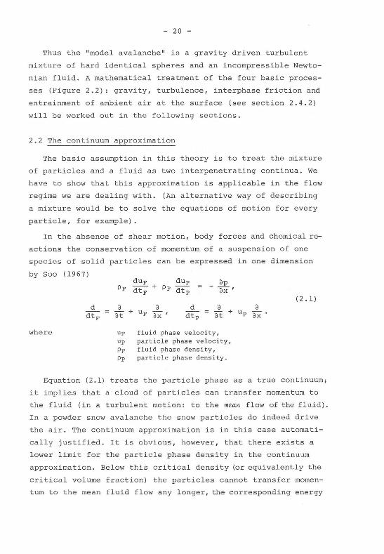
DFs Dt

0,

(2. 29)

us where ~s = <w

5) is the velocity of the (geometrical) surface.

In this surface the field variables may have finite jumps. We

de6{ne the avalanche surface as the locus where the particle

phase volume fraction is discontinuous. It has some finite va­

lue inside the avalanche, outside it vanishes id·~ntically. This

is a reasonable definition since we can see (Figure 2.5b) that

there is a sharp edge. In terms of (2.11) and (2.12) we have

For the particle phase, (2.11) then reads

~(2)- • ~n = ~s ·~n ·

( 2. 30)

( 2. 31)

So, the surface is material for the snow particle phase. Com­

bination with (2.29) yields

<! z 5 + azs u.( 2 )

at ax (2) - w 0, ( 2. 32)

From now on we omit the "-" indices. A field evaluated at

z = zs without "±" index means that the surface is approached

from the "-" region (Figure 2. 5a).

The jump condition (2.11) for the air phase reduces to a

relation akin to (2. 32). Since c+ = l and because of (2. 31) it

reads

where + E=-(~(l)

-E

(?)+ - ~- )

azs 2 l+(axl, at z=zs· (2. 33)

·~n (2.34)

is called enbr.iU11111en.t Jta.te. E· p (l) is the flow of air mass per

unit time and per unit area through this boundary. It is func­

tionally rela ted to the turbulent structure or the flow and

must be formulated as a further constitutive quantity besides

the Reynolds stresses and the momentum transfer (see equations

- 33 -

2.27). We still have to exploit equation (2.12) at the ava­

lanche surface . Applied to the snow particle phase this equa­

tion y ields in combination with c(2)+ = 0, and (2 .16) (see Schei­

willer & Hutter , 1982, p. 63)

[ (2) (2)EJ ~ t(2)E c P - txx () x + xz 0 , ( 2. 35a)

c ( 2) P + tx( 2z) E ~ + t ( 2) E ax zz

a t z = z5

0 . (2. 35b)

For the air phase the corresponding conditions are (Scheiwiller

& Hutter*!, 1982, p . 63/64)

(2. 36a)

c<ll w<ll ozs + u (l) azs - w<ll) <at ax

l ii (l) [

+ (l) (l)E az5 (c p+txz ) ~ (2. 36b)

ozs 2 l+ <--a;zl ,

where

is the air velocity i mmediately above the avalanche surface.

E, Kx, Kz cannot be chosen independently of each other , since

they are related through the definition of the entrainment rate

(2. 34).

§ggg!!l_~9f!~l~~!f-~9!!~!!~

In principle we could go through the analysis as for the

surface with interchanged roles for the snow and air phases:

The bottom surface would be material for the air phase, and

there would be an entrainment rate Esnow f::Jr the snow particle

phase.

We shall ignore this snow entrainment and require no-slip

at the bottom, so that

*) The expressions in Scheiwiller & Hutter (1982) are in error due to a slip in calculation .

- 34 -

u<ll = w<ll = u<2l = w<2) = 0, at z = z8 (2.3 7 )

If we also allow for discontinu i ties of the volume fractions,

this implies [through (2.12)] that

p+ = p(z = zs) = 0. (2. 38)

An important characteristic of a turbulent fluid is a large

amount of vorticity . The entrainment process at the edge of a

jet (for example) is the cause for the deve l opment of vorti ­

city in a previously irrotational fluid; this development de ­

pends strongly on v iscous diffusion of vorticity across the

bounding surface (Townsend, 1980). We do not intend to describe

microscale processes at the surface, but rather suggest a re ­

lation between the entrainment rate E and mean pressure and

ve locity fields . The first approximation to the entrainment

process has been made by assuming the surface to be a func ­

tion z 5 (x, t) . What we are· describing by zs (x, t) is in fact some

averaged surface. In turbulent shear f lows the surface is

usually folded (Townsend, 1980) Next we tacitly assumed that

the surface, defined by the turbulence, is the same as defined

by the jump in the snow phase volume fraction . This is a useful

approximation of the mean location of the surface.

In most boundary layer theories with an entrainment-closure

the entrainment rate is a (usually linear) function of a cha­

racteristic boundary layer velocity (for example maximum ve lo­

city, mean velocity). We a lso allow for dependencies on pres­

sure and cross - stream velocities and suggest

E (u(l)+ - ~ (2)+ ) 1 ·en= El(P-Pa l+E2 u<ll + E3w(ll, lz=zs

( 2 . 39)

at z=z 5 •

It will turn out (chapter 3) that var i ations in the entrainment

modeling will influence the solution very weakly only. This is

reasonable because a small increase in a i r mass has little

effect on the total mass which is control led by the amount of

- 35 -

snow mass present. Moreover, no significant gradients in the

mean thickness at the avalanche body are observed, thus giving

further evidence that, once the avalanche has developed, the

entrainment is no longer the crucial mechanism.

2.4.3 Complete mathematical formulation

The summary of field equations and boundary conditions gives

ac< 1 l ~· (c(1) ~(1)) 0, a t

+

a c<2l - -+

at ~· (c(2) ~(2)) 0,

1 - ( 1) p ( 2) 112 1 p(1)~(c p)+CFric(p(1)) -r

c (2) • ( ~ ( 2) - ~ ( 1) ) + c (J) ';! +

1 a () u< 1 l + - ( 11 (1) --;;-z ) '

p(1) dz t 0

a ( c(2) u< 2l) - (2) (2) 12) at- + ~ • ( c ~ l'l ~ • l

1 p(1l 112 1 p(2) ~(c(2 ) p) - CFric (p(2)) -r

. c(2) ·(~(2) _ ~(1)) + c(2) g +

1 _i__ ( , <2l a ~<2l l + p(2) az '"'t az

"t(ll - c<1l -P(1) c(1) k(1)2 ... - \l ~·

\l~2l c;/' p<2l c<2l k£(~~~,

P-(1} (1} dk(l}

c dt

P- (2} (2} dk( 2

} c dt

r (1) ~k(1ll a l(llt + \l(1)) _o __ + azLcrk<ll azJ

au (ll 2 ak< 1 ll(2 2 + \l~1l ( -az l - 2v(az-l - £ {1)'

a r llt(2

} (2} ak<2l ] azL(crk<2> +\l az +

(2} ou<2l 2 ak(2ll!2

2 (2} + llt (- --) - 2v(-,- -) -£ ,

()z oZ

(2. 40)

cont._,.

- 36 -

dc:(l) a [ llt <I> (l) l p( l} c(l) (l))~

dt - ( - -+

\1 az J + az crc:(l)

+ c<l> c:< l> \1 (l) au<l> i5 (l) c<l> E (1)2

t <--->2 _ c<l> l k(l) az 2 k(l)

P(2) c(2) dt:(2} a I llt<2> <2> ac:<

2>J

dt az L crc:<2> + \1 ) ---az +

+ c<2> c:< 2> llt<2> au<2> 2 (2) i5(2) c(2) E(2)

l }: (2) ( az ) - C2 k(2)

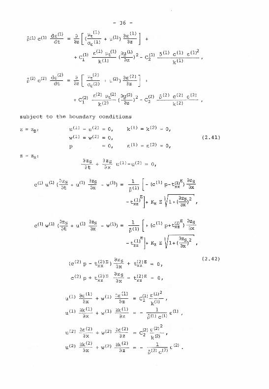
subject to the boundary conditions

u<1) = u<2) = 01 k(l) = k(2) = 01

w<l) = w<2) 01

p = 01 E (l) = c:(2) = 01

z = z5 : azs azs

u(l >-u< 2> 01 --+ ax = at

(l} (l) ( 3zs + u<l) Clzs - w(l)) C U Tt dX

- (c< ) p-t<l) ) -1 [ 1 E Clzs p (1) XX dX

u(l) Clt:(l) + w( l) Clx

u<l) ak< l> + w( l) ax

(lc:(2) u<2) + w<2)

ax

u<2) :lk (2)

+ w<2) ax

El Clzs 2 - t~~ ) r Kx E 1 + <ax-> I

-t(l)E]+ K E zz z

azs 2 1+<-ax> I

az 5 ax

~ E (1)

Clz

ak(1)

Clz

(lc: (2)

Clz

ak< 2> az

0'

t(2)E zz 01

(l) E (1)2 c 2 -k_(i) 1

- 1 (1) i)(l) c(l) c:

2 (2) E (2)

c2 "k<2l

1 E (2) p<2) c<2)

(2.41)

(2. 42)

- 3 7 -

If we want to l ook at a transient problem, we have to pro­

vide initial conditions. In the following sections we will dis­

cuss a technique of finding steady state solutions.

2.5 The steady- state problem and it s significance

It is not obvious that the system (2.40), (2.41), (2.42) admits

a steady-state solution at a ll. For exampl e, if there is a time­

dependent supply of snow- air mixture from a reservoir upstream,

the solution is certainly transient. A real powder - snow ava­

lanche is a transient phenomenon too. But the steady-state so­

l ution , given a constant material supply from upstream (Figure

2.6), is easy to obtain from a computational point of view. More­

over this process may be simulated in the laboratory (see Schei­

willer, Bucher & Hermann, 1985). This way it is possible to check

the accuracy of the underlying assumptions and approximations .

Reservoir tvi th snow- air mixture

Figure 2.6

Steady laboratory avalanche forced by steady influx of mass.

2 . 6 Kantorovich-technique

2.6 .1 Basic idea

There is no principal new

difficulty in integrating the

system (2.40), (2.41), (2.42)

for a transient situation,

except for numerical and com­

putational complications .

The goal in computing the

steady state solution is to

test the mathematical model,

that is to test whether the

basic processes turbulence,

entrainment and interphase

friction are mode l ed appro­

priately.

In jet theories (or boundary or mixing layer problems in ge­

neral) it is very common to integrate and thus average the lo­

cal balance equations in the cross stream direction, because

two- d imensional numerical solutions would r equire a large amount

- 38 -

of computer facilities. The differential equations emerging

from this procedure are one-dimensional in space. The steady­

state problem is then governed by ordinary differential equa­

tions. However, a serious short-coming of this procedure is the

loss of information about the cross-stream variation of the

fie lds. The method of integrated balance equations thus is not

always adequate (see section 2.1). But there exists a more ge­

neral technique for the treatment of quas i-onedimensional flows,

namely the method of weighted residuals (Kantorovich & Krylov,

1958, Raggio & Hutter, 1982), subsequently also referred to as

Kan-toJtovieh technique. The basic idea of the Kantorovich-technique

is to expand every field variable ~ (x,z,t) (velocity components,

volume fractions, pressure, turbulent kinetic energies, dissi­

pation rates) in the cross-stream direction z in a series of

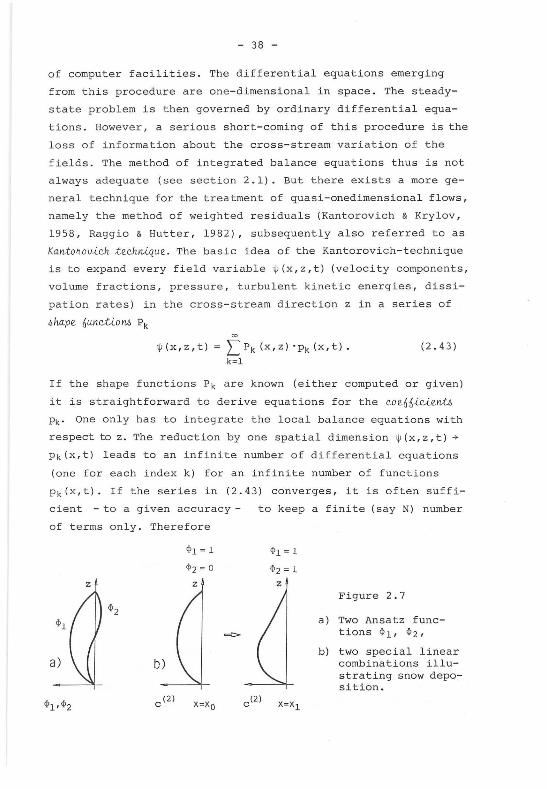
~hape 6unetio~ Pk 00

~(x,z,t) Lpk (x,z) ·pk (x,t). k=1

(2. 43)

If the shape functions Pk are known (either computed or given)

it is straightforward to derive equations for the eoe66ieie~

Pk· One only has to integrate the local balance equations with

respect to z. The reduction by one spatial dimension ~ (x, z, t) +

Pk(x,t) leads to an infinite number of differential equations

(one for each index k) for an infinite number of functions

Pk(x,t) . If the serie s in (2.43) converges, it is often suffi-

cient - to a given accuracy -

of terms only. Therefore

z z

b)

X=Xo

to keep a finite (say N) number

<1>1 = l

<1>2 = l z

Figure 2.7

a) Two Ansatz func-tions <1> 1, <l>z,

b) two special linear combinations illu-strating snow depo-sition.

c(2) X=X1

- 39 -

N

lj!(x,z,t)::::: L Pk(x,z) Pk(x,t) - Pk(x,z) Pk(x ,t). k=l

(2. 44)

This approximation is (for fixed N) the better, the better

the shape functions Pk are chosen. As an example, let's take

N = 2 and look at a typical snow volume fraction profile. The

two shape functions w1 , w2 are given (Figure 2.7a). The volume

fraction is then (2)

c(x , z) = w1 (z} cp 1 (x} + w2 (z) cp 2 (x), (2. 45)

where the shape functions have a z -dependence only, for sim­

plicity and the situation is assumed to be steady.

We can model the deposition by (see Figure 2.7b)

1

0 +

1.

1.

2.6.2 Kantorovich-transformed system of equations

As an example the Kantorovich-transformation for the air

mass balance is worked out thoroughly. All other balance equa­

tions are treated in an analogous manner. Starting from (2.40)

and neglecting time- dependencies yields

0. (2. 46)

Consider the expans ions

c(l) (x,z) (1) (1) ei (x,z)· ei (x),

u(l) (x,z)

(2. 4 7) w(l) (x,z)

69- (l) (x,z) (1) (1) Ai (x,z)·Ai (x),

where 69- (l) is a weighting 6u.nc.tion, and the functions e{ l), S1 i l),

'¥{1), Ai1l, i=l, ... , N are the given shape functions. The

weighting function is arbitrary, but is also assumed to be ex­

pandable according to (2.47 d).

- 40 -

The following procedure is now carried out: The balance

equation (2.46) is multiplied by the weighting function 6£(1)

and the resulting equation is integrated over the whole inte­

gration domain. In this process the a;az-term can be integra­

ted by parts. This yields

J r }x<c<1l u<1l) o£( 1) dz dx - f f5 c(1) w<l) a~~( 1 ) dz dx

X 0 X 0 (2. 48)

+ f [ c< 1) w<l) o£< 1) J : ::s dx = 0. X

For the term in square brackets, substitution of the time-in­

dependent form of boundary conditions (2. 33) and (2. 37) yie lds

f c(1)w(1)o£(1)]z =zs = o£( 1)·(E· l+( azs )2+c(1)u(1)3Zs)l . (2.49) L z=zs ax ax z=zs

Therefore, upon substitution of (2.47), (2.48) becomes

zs zs

f [<Je<1) n< l) f1(1) dz)·1....(e(1) w(l)) + f l(e(l) n<1)) /\( !) dz-e\1) w(l) i j k ax 1 J ax J k k 1 J

X 0 0 zs (1)

- Jei1l'!'~1 l a~~ dz-e{ 1 lljij 1 l+/\~1l(z=zsl·E· l+(a;:l2 (2.50)

0

+ e?)(Z =Zg) nJ 1 )(z=Zg)· /\~1 ) (z=zg)·8i1 ) wj1) aaz:] o,\~1 ) dx = 0.

Since ( 2. 50) holds for any arbitrary choice of 6 ,\~1 ) (x), k = 1,

... ,N, the term in square brackets in (2.50) has to vanish for

each k, individually, that is

l:r-1(1) ~(e (1) w(l)) + 21·1(1~ 8(1) (1) 3 8 ~1) 1jJ (1) w. + lM ij k 1] k dx 1 J 1] 1 J 1 J

(2. Sl a )

41M(1~ 8<.1) w(1) ~ 5 l+ (~;)2 = 0, + + J.1k ·E· k = 1, •• . , N,

1] 1 J

where

(2.5lb) 2

:Mijk (x)

cont.-+-

- 41 -

- Jzs 8 (1) '!'(1) ai\k(1) 1 J --az- dz,

0

8 l1J nj1l 1\~1) J ,

lz=zs

5 lMk (x)

(1) 1\k (z = z5).

The expression needs further explanation. If we set

-for example - in (2.39) E1 =E 3 =0, then

where 5JM-(1) (1) (1)

jk = '!' j (z = z5 ) · 1\k (z = z5 )

The equations (2.51) are a set of N ordinary non-linear

differential equations with variable coefficients. They have

the form of an initial-value problem in x - space.

The coefficients hiM{~~ depend implicitly on z 5 . Simplifica­

tions emerge with the coordinate transformation

I; =

that leads to

z ZS'

zs

di; = dz zs

F(x,z5 ) = f f(x,z) dz

1 0

z 5 • J f(x,zs· l; ) dE; 0

valid for each of the integrals.

1

z5 • f f (x, i; ) di;, 0

(2.52)

The above procedure of reducing the air mass balance is car­

ried out for all balance equations listed in (2.40), with the

expansions

c( 2) = 8{ 2l (x,z). e{ 2) (x)'

u(2) = n(2) (x,z). w( 2) (x)' l l

w(2) = '!'(2) (x,z). ljJ(2) (x), l l

p(x,z) = lli(x,z) · ni(x),

(1 2) (1,2) )Jt ' (x,z) = ri (x,z). y i(x)'

E (1 , 2 l (x, z)

k( 1 , 2 ) (x,z)

1'1(1,2) (x,z) 6(1,2) (x)' l l

<1,2) (x,z) K{1,2) (x).

Through cumbersome algebra, summarized in Scheiwiller (1984),

one obtains finally (using the same weighting functions in eve­

ry equation) •

- 42 -

k ;:::.1, • •• , N, ( 2:53 a)

+ 3:.1(2kl e(2lw(2l ~ + 41M(2kl e(2)t/1(2l 0 q 1 J d X l.J 1 J '

where zs l "'(2)

ijk J 8{2> nj2> Ak dz,

0

2 lM (2) zs f .l (8(2) n(2l ) A dz, ijk ax 1. J k

0

31M(2~ 8i2> n(2l Ak I , l.J J z=z 5

(2.53b)

41M(2~ zs aA k -f 8(2) '1'(2) - - dz l.J 1. J az

0

as mass balance for the snow particle phase,

+ 8 ru (1) ,,(1) e(1) w~ 1) + 9ru (1) y(1) w(1) l0ru (1) ~~-~ e(l) w(1) w(1) hijk "'h 1. J l.Jk 1. J + hijk dx 1. 1. J

ll (1 ) dzs e.(1l rr(.1 l + l 2ru(.1.kl ~d~~ y.(1l w(.1l + l3ru(1 ) dz~ (1) dw/1

> + ruijk -d.x 1. J l.J x 1. J ijk dx Yi - ax -

l4ru (1) ~:_s_ Ez 0, k = 1, .. . , N, + k dx (2. 54 a)

where zs 1 ru (1) f n (1l .1.(8( 1 ) n( 1 l ) A dz, hiik h ax 1. J k

0

Zru(ll zs

hijk J n~u ei1

l n ;1

> Ak dz,

0 (2. 54 b)

zs 3DJ (l~

J 0( 1 ) n Ak dz, l.J p (l) 1. J

0

4ru(l~ zs J .l.. (0 (ll n . ) A dz, l.J p( l) ax 1. J k

0 cont. +

5:ru (1) jk

8DJ(l) hijk

- 43 -

zs

f (1)

- g sin a 0j J\k dz,

0

0( 2 ) 11( 2 ) J\ dz 1 J k

zs CFr1· c p· ( 2 ) 1/2 f (2) (l)

- -- -(- --) 0i rlj J\k dz, 1: p (l)

0

zs - f _a-("'(l)' ) 0(1) ,.,(l) d

dZ T h "k 1 HJ Z >

0

l zs (1) ai1J.<1l ai\k

-=--(i) J 1 i az- - a:l dz, p 0

0(1) IT J\k 11 ,

p(l) 1 J z=z5

~" (1) (1) OHj I

- - -- I i --;;·x·- Ak z=z , p (1) 0 s

r (l) "(l) J\ I , i "J k I p(1) z=zs

zs

r J\k dz , p (l) )

0

as downslope momentum ba l ance for the air phase,

l 1Whn1_Jlk <ll _cl_(e<1l lj!nl) + 21W<1l. w.<1l. e<1l lj!<1l + 31W<lk) e<2l lj!<2l

wh dx i j h1]k ··n 1 J 1J 1 J

sJW (1) 6

(1) + 61W (1) lj!h<1l 6 (1) lj! (1) + j k j h1Jk 1 J

(2.55 a)

0, k = 1 , ••• , N,

where

51W (1) jk

61W(l) hijk

71W (1k) ~J

- 44 -

zs

J n2> 0i1l 'I' ;1> Ak dz' 0

zs ( ,.,( 1) -~ ( 0 (1) '1' (1)) A d ; " h ax "i j k z •

0

C (p<2l)if2 -.1-- Jzs 0 ,(2)'1'J(2) Ak d - Fric -:-(IT , ~ z,

p 0

zs

g cos a J 0{1> Ak dz, 0

zs - J -~ ( '1' (1) A ) 0(1) '1' (1) d

az h k i j z • 0

- _1 ___ Jzs 0( 1) Jl. -~ A_I5_ dz - < 1 l ~ J az ' p 0

zs (1) a'!' j<1> aA k ::·n> f r i - ·ai -- -a z dz, p 0

0~1) nll) '1' ~1) Ak lz=z s

as vertical momentum balance for the air phase,

lru <2> <2> ..:!._(8 <2> <2>)+ 2n.1 <2> 8 <2> <2> hijk wh dx ~ w J hijk wh i wj

(2 . 55 b)

(2. 56 a)

cont . +

- 45 -

10 ru (2) dzs eh(2) w (2) (l\ (2) + 11 ru (2k) dzs e(2) 1T· + hijk dx 1 J lJ dx 1 J

2 dw· (2 ) 13 + 1 ru1( 2J·k'· (2) _ J ___ + ru (2kl (2) (2) 0,

where

y i dx lJ y i wj

1 ru (2l hijk

2 ru u' hijk

6 ru (2, ijk

9 ru (2kl l J

11 ru (2kl lJ

12ru( 2kl lJ

13 ru (2 J ij k

zs J n~2l 0 i2l n~ 2l '\ dz,

0

zs

f ,-, (2) l_- {0(2) >1(2) ) A d " h ax l J k z'

0

p(l) 1/2 - CFr i c (-=- (:2) )

p

zs - J .l_ ( '¥ ( 2 l A ) 0 ( 2 l Q ( 2 l dz az h k 1 J •

0

_ __ 1 __ _ (2) A - (2l 0i rrj k I , p z=z 5

k = 1, •. . IN ,

(2.56b)

as downslope momentum ba l ance for the snow particle phase,

- 46 -

1 JWh<~J>k <2> ~ ( 6 <2> ,, <2>) + 2 ~~~ <2> w c2> 6 <2> 1ji <2> + 3JWJ<k2> 6 Jc2> ~ ~ dx ~ "'J hlJk h '- J

4JW<2k> 6 c2>,,< 2> + 5IWc2k> 6 c2>,,,cu 6JW<2> 1jih<2> 8 <2> 1ji <2> ~J ~ "' J lJ ~ "' J + hijk ~ J

where

3 ., (2) "'jk

5 lW (2k) ~J

6 ., (2) "'hijk

l 0 JW(2k) ~ J

0, k = 1, ... IN,

zs J ~~~ 2) 0 ~ 2) '!' j Ak dz ,

0

zs

J nh<2> .1_ (0<2> '1'<2> ) A d ox l J k z,

0

zs f 0J

2> Ak dz,

0

0 (l) zs (E -)1/2 J. f 0C2l 'l'C2l Ak dz

0 (2) '( l J , p 0

i5 (l) 1/2 - CFric (-.:(2))

p

zs _l_ J 0(2) 'l'Cll Ak d '( ~ J z,

0

zs - J _d (w(2 ) A ) 0(2) '1' (2) d

oz 'h k ~ J z, 0

zs oAk

f 0~2 ) nJ. -;;-z- dz,

i5 (2) 0 0

zs (2) r <2 > o'l'J oA k J r i -,z- OTz- dz,

i5 (2) 0 0

(2 . 57 a)

(2 . 57 b)

as vertical momentum balance for the snow particle phase,

where

- 4 7 -

1 1b(1k,2) (1,2) 0(1 , 2) 1) y i j +

2Q;(1,2) 6 (1,2) K(1,2) K (l,2) = Q , h ij k h 1 J

1 ~(1 , 2) ijk

2,.. (1 , 2) ""hijk

k = 1, ... , N ,

zs

f r }1 , 2) A (1 , 2) A d ~ "j "k z,

0

zs

C(1, 2) .(1, 2) ( 0 h(1,2) K(1,2) K(1,2) A d • IJ p J i j Ilk Z I

0

for the turbulent viscosities ,

(2 . 58 a)

(2. 5 8 b)

+ 1 D<(1, 2) 6(1,2) hijk h

(1 , 2) (1 , 2) dKj

w. - ···- - ·-1 + 2 IK( 1, 2)

8<1 ,2) (1 , 2) (1, 2)

hi j k h wi • Kj d x

+ 3 D<(1, 2) (1 , 2) (1,2) (1, 2 ) 4 D< (1 , 2 ) (1, 2) ,,(1 , 2) ,,,( 1,2) hijk Yh · wi wj + hi jk Yh "' i "'J

+ 5 D((1,2) 0 (1,2) + 6 D((1~ 2) 8

(1,2) \).1(1 ,2). K(1,2) + 7 D((k1,2) . K(1 ,2) jk J hl)k h 1. J J J

+ 8 D< (1 , 2) . (1,2) (1,2) ijk yi Kj

+ 9 D<(1, 2) 8(1,2) 0(1 , 2) ijk l J

(2 . 59 a)

d K (1 , 2 ) 11 + 10D< (l , 2) 8

<1,2l_ w (l,2J _j__ D<(1,2) 6

<1, 2) (1 , 2) (1 , 2) hijk h '- dx + hijk · h wi Kj

+ 1 2 D( (1 , 2). (1, 2) K( 1, 2) ijk y 1. J

0 , k = 1, ... , N,

where

1 D< (1 , 2) hijk

2 D< (1,2) hijk

3 D<(1,2) hijk

4D<(1,2) hijk

5 D< (1,2) jk

zs f 0~1,2) ni1, 2 ). K~1 ,2) Ak dz,

0

3K .<1, 2) _J __ Ak dz,

3x

zs 3n,<1, 2) 3st(l , 2J

f r{l, 2 ) ~ _L_ Ak dz, p <1, 2) h 3z 3z

0

z 5 3'1'<1,2)

3'1' (1, 2 )

J, r <1,2). _ _ i __ J __ Ak dz,

- .(1,2) h 3z 3z p 0

zs _1_ J 6(1 , 2) Ak dz, • (1,2) J p 0

(2.59 b)

cont. -+-

61K(1,2) hijk

71K (1,2) jk

SIK (1,2) ijk

91K(1,2) ijk

10 IK (1,2) hijk

11 IK (1 , 2) hijk

12 IK (1,2) ijk

- 48 -

zs

f 1._(8 <1,2) '1' (1,2) .fl) K(1,2) dz, a z h 1. k J

0

zs aflk aK.< 1, 2l

_ll_ J """z-. ~z dz, ii(1 ,2 ) 0 0 0

8(1,2) ·6(1,2) fl I . 1. J k z=zs

- 8(1,2) 11(1 ,2) K (l' 2) flk I h 1.

J I z=z s

8(1 , 2) 11(1 , 2) ad1 , 2)

flk I z=zs' J

h 1. ax

. r <1,2) aK<1,2)

flk I - - - ------- --- J

0 (1 , 2) p( 1,2) 1. --a-z--lz=z5 k

as balance for the turbulent kinetic energies,

do' 1 ' 2 l 2 1 lE(1,2 ) (1,2) 9 (1,2) (1,2) --~--- - + lE (1,2) (1,2) 9 (1,2) (1,2) 0 (1,2) ghijk Kg h wi dx ghijk Kg h wi j

+ 3 lE (1 , 2) (1,2) 0 (1,2) (1,2) (1,2) ghijk Yg h wi wj

+ 4][(1,2) (1,2) 0(1 ,2) ljJ(1,2) ljJ(1 , 2) ghijk y g h i j

5JE<1,2) 9 h<1, 2l 6,<1,2) 0 <1 ,2) + hij k ~ J

6 lE (1,2) (1,2) 9 (1,2) ,,( 1,2) '(1,2) + ghijk Kg h '1'1_ UJ

+ 7 lE (1 , 2) (1,2) (1,2) 0 (1,2) hijk Kh y i J

alE <1,2) <1,2) 6 (1,2) + ijk Ki J

(2. 60 a)

+ 9][(1,2) (1,2) 9(1,2) ,,,(1, 2) 0 (1,2) 10][ (1,2) (1,2) (1,2) 0(1,2) ghijk Kg h '~'i j + hijk Kh y i j '

where

1 lE(1' 2) ghijk

2 lE(l,2) ghijk

zs

f K ( 1' 2) G ( 1' 2) Si ( 1 '2) 6 < 1' 2) flk dz ' g h 1. J

0

zs

J K < 1' 2) 8 < 1' 2) Si< 1' 2) a6 j flk dz,

g h 1 ax 0

k = 1, ... ,N,

(2.60b)

cont. +

31E(1,2) ghijk

41E(1,2) ghijk

5 IE(1,2) hijk

61E(1,2) ghijk

71E(1,2) hijk

81E(l,2) ijk

9 IE(1,2) ghijk

10 IE (1,2l hijk

- 49 -

c1<1,2) zs ()1)(1,2) ()1)~1,2)

f 1'(1,2)6(1,2) 1 J 1\ dz, ii(1,2) g h az az--

0

c1<1,2) zs ()ljl (l,2) 3'¥ (1,2)

f r (1,2) 6~1,2) 1 __J __ 1\k dz,

ii(1 , 2) g az az 0

zs C2

(1,2) f 8

h(1,2) 6

(1, 2 ) 6

(1,2) J\ d i j k z,

0

zs - f _a (K<l,2l 8 (1,2) '¥<1 ,2) Ilk) 6 d

az g h i j z • 0

z5 06_<1,2)

-- --·-- - - - J _1_ (K(1,2l 11 ) r <1,2l _ J dz, 0

(1,2) • (1 , 2) az h k 1 az k p 0

~ (1,2) Zs

J jl_ (K(1,2) 11 ) 6(1,2) d

< 1 2 l az 1 k J z' ii ' 0

K(1,2) 8 (1,2) '¥(1,2) 6 (1,2). I g h i j Ilk z=z ,

s

for the dissipation rates of the turbulent kinetic energies.

It was mentioned before that the weighting function o~ and

thus also 11p> are arbitrary. However, the choice is not comple­

tely free, because at every x = x 0 a non-singular system of

equations should emerge, this system of equations being defi­

ned by the coefficients (j)..,(i), (j)ru(i), (j)JW(i), •••• Moreover, the

value of the weighting functions at the surface z = z 5 must be

chosen carefully. For example 1\k (z = z5 ) = 0 would imply 5 JM~l) = 0

and thus the entrainment term would be eliminated from equa­

tion (2.51). This would not be reasonable, because entrainment

was supposed to be important.

The Kantorovich-technique is a generalization of such well

known methods as finite difference and finite element methods.

- 50 -

The choice

yie lds a multi-level model , the choice

l Zk :S Z :S Zk+l

0 elsewhere

yields a mult i-layer model. In fin ite element techniques the

J\ -functioas are usually piecewise linear . In the case N = l, the Kantorovich-technique turns out to be a construction of

similarity so lutions. (2.44) is then simply a separation an­

satz.

2.7 The finite difference technique

The reader is supposed to be familiar with the features of

the finite difference (FD) method (for details see for examp le

Smith, 1978). The computer code PHOENICS (Rosten and Spaldinq,

1981; Rosten , Spalding and Tatchell, 1981) used here was deve l ­

oped by CHAM Ltd . London. PHOENICS solves three-dimensional

transient two-phase flow prob l ems . The spatial discretisation

is represented by a staggered grid (Figure 2.8).

There is a finite difference (algebraic) equation for each

variable for each control cell (Figure 2.8) in the domain of

integration . These equations are just the integral balances

+ + +

+ + +

+ %1); +

+ + +

+ + +

I

+ +

+ +

+ +

+ +

+ +

• Locations, where the velocities are compu ­ted

+ Locations, where all other var iables are computed

0 "control cell" or Figure 2 . 8 "domain•'

Staggered grid in two dimensions .

- 51 -

within the control cells. They may be written in a quasi ­

linear form , but are in fact non- linear because the coeffici­

ents are functions of the variables. These numerous (up to

several thousands) strongly- coupled equations are solved by

an iterative predictor- corrector procedure.

The finite difference equations are formulated fully impli­

citly (see Smith, 1978) . Advective terms are obtained by up ­

stream- differencing (Rosten & Spalding, 1981) in the stagge­

red grid .

The full implicitness guarantees numerical stability. The

turbulent stresses in the fluid phase are calculated by means

of the k - E- mode l (see section 2.3 . 3) , turbulence in the par ­

tic l e phase is neg l ected . Resu l ts wi ll be presen ted in chap­

ter 3.

- 52 -

3. Laboratory simu lation of powder-snow avalanches

3.1 Similitude and experimental set-up

In this chapter the small-scale laboratory simulation of

powder - snow avalanches is described (see Scheiwiller , Bucher

& Hermann, 1985) . As the motion of real powder-snow avalanches

is governed by gravity , turbulence, entrainmen t and interphase

friction (see chapter 2), a laboratory flow must be created in

which these four mechanisms play crucial roles. The fact that

interphase frict ion operates, presumes that the flow is suspen­

sion- like. Existence and stability of a laboratory suspension

depend upon the material density and the size of the parti cles.

The smaller the particles are , the more likely they will stay

in suspension, because, i f the dens ity is assumed to be given,

the gravity force is a function of the pa r t icle volume, whereas

the friction i s a function of the particle surface . However,

fo r ve ry small particles, gravity is too weak to induce and

maintain a fully turbulent flow. After preliminary experiments

(with sand of different grain sizes, graphite powder etc .)

choice was made to perform the simulation by substituting the

air by water and the snow particles by polystyrene particles~.

The po l ystyrene particles have a density of 1.25 gcm-3 and a

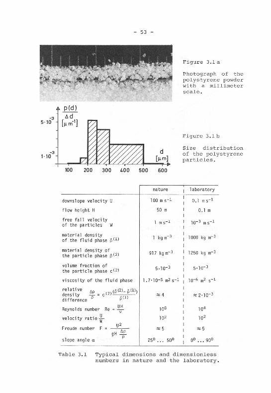
size distr ibution between 200 and 400 ~m (see Figure 3.1).

The similarity between the real powder - snow avalanche and

that in the laboratory is basically due to the conservation of

a densimetric Froude number and the veloc ity ratio U/W (see

Table 3 .1). The Reyno l ds number is for both natural and labo­

ratory ava l anche very high and therefore insignificant .

The basic equipment needed for such a suspension flow down

a s l ope in the laboratory cons ists of a basin f illed with wa­

ter , a submerged chute , a feed apparatus and e l ectronic compo­

>ents (see Figure 3 . 2).

* ) They are commercially available as Schaettifix No. 374, 200- 400 ~m, Schaetti & Co ., Wallisellen, Switzerland.

- 53 -

'' ., . . \ .

. ,· '

-3 5·10

-3 1·10

100 200 300 400

downslope velocity U

flow height H

free fall velocity of the part icles w

material dens·i ty of the fluid phase ii(l)

materia l density of the particle phase p(2)

volume fraction of the particle phase c<2)

viscosity of the f luid phase

re l ative l1P (2) (p (2)_ ii (1)) density p-= c ,;<1) di fference

Reynolds number Re UH =v

velocity ratio ~ Froude number F =

U2

-;tiP g -slope angle a

p

500 600

nature

lODms-1

50 m

l m s-1

l kg m-3

917 kg m- 3

5·10-3

l. 7·10-5 m2 s-1

~4

lQB

102

"='5

25° .. . 50°

Figure 3.1 a

Photograph of the polystyrene powder with a millimeter scale.

Figure 3.1 b

Size distribution of the polystyrene particles.

laboratory

0.1 ms-1

0. l m

10-3 m s-1

1000 kg m-3

1250 kg m-3

5 ·10-3

10-6 m2 s-1

""2·lo-3

104

102

"='5

oo ... goo

Table 3.1 Typical dimensions and dimensionless numbers in nature and the laboratory.

GANGWAY 0

- 54 -

TRANSDUCER <D WATERPROOF BOX WITH}®

STEP-DRIVE MOTOR MICROPROCESSOR @

CHUTE @ TANK ®

BOTTOM OUTLET ®

FEED APPARATUS ® INTERIOR STEEL FRAME ® EXTERIOR STEEL FRAME @)

Figure 3.2

General experimental set up: water tank, chute, feed apparatus, transducer with driver and controlling computer.

The only dimensionless number which differs by orders of mag­

nitude between the processes in nature and laboratory is the

relative dens ity difference. This is not a serious deficiency

at least as far as the field equations are concerned, because

the density is always coupled with gravity which is accounted

for in the densimetric Froude number. However the relative den­

sity difference might have a reducing effect upon the entrain­

ment rate (Tochon-Danguy, 1977). The free fall velocity W is

a good estimation for the velocities perpendicular to the wall.

- 55 -

One could include the slope angle in the Froude number by

2 /',p . writing F = U / (gH -ps1ncx), but to maintain this invariant

the slope angles in nature and in the laboratory would no lon­

ger have to be the same, which is rather dubious and unsatis­

factory. If we thus assume a similitude that is based on the

conservation of ex , G = _Q_

w and

the stretching factors are roughly

V nature R,nature

V laboratory R-laboratory

F u2

__ /',_ p_

gH p

(6 p) P laboratory

The laboratory suspension flows down a 30 cm wide flat chute

with perspex walls (see Figure 3.3 a). It is 3 m long and enti­

rely submerged in water, within a tank of 5m x 4m x 1. 5 m with

front windows (see Figure 3.3b). The inclination of the chute

may be selected arbitrarily between 0° and 90°.

The two-phase mixture is prepared in a 1 m high vertical

cylindrical tube with a faucetted bottom (see Figure 3.4). The

suspension i ssues with a velocity of about 35 cm s -1 through

Figure 3.3 a

Submerged chute with perspex walls and head of a laboratory avalanche.

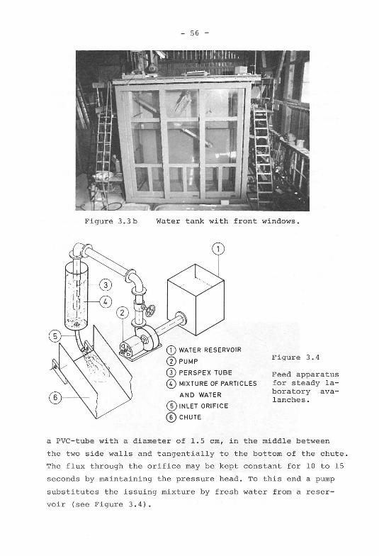
Figure 3.3 b

- 56 -

Water tank with front windows.

CD WATER RESERVOIR

Q)PUMP

G) PERSPEX TUBE

(0 MIXTURE OF PARTICLES

AND WATER

®INLET ORIFICE

®CHUTE

Figure 3.4

Feed apparatus for steady la­boratory ava­lanches.

a PVC-tube with a diameter of 1.5 cm, in the middle between

the two side walls and tangentially to the bottom of the chute.

The flux through the orifice may be kept constant for 10 to 15

seconds by maintaining the pressure head. To this end a pump

substitutes the issuing mixture by fresh water from a reser­

voir (see Figure 3.4).

- 57 -

The time of 10 to 15 seconds is sufficient for the transient

avalanche head to pass the transducer that records velocities

and densities. The tail behind it is steady, except for the

turbulent fluctuations which are always present in these kind

of flows. Profiles of particle phase velocities and particle

concentrations are obtained by an ultrasound technique (the me­

thod for pointwise measurements is explained in sections 3 . 2

and 3.3). The ultrasound transducer is pulled perpendicularly

through the laboratory avalanche, stopping successively at 16

positions fo r a pointwise measurement of particle phase velo­

city and particle concentration. The transducer-driving step­

ping motor is protected by a waterproof perspex box, because

it is attached to the chute and submerged . The axle is sealed

by surrounding it with flexible rubber bellows (see Figure 3.5).

The stepping motor is controlled by a microprocessor which

also collects and processes the data . The maximal distance

which may be covered by the driving mechanism is 30 cm. In the

experiments profiles were

taken from 0.5 cm to 19.5 cm

above the chute bottom, at

16 equidistant points. It

was not possible to measu­

re nearer at the bottom,

because the head of the

transducer is 0.8 cm thick .

A profile measurement takes

roughly 3 seconds. The

transducer is moved back to

its initial position and

the next laboratory ava­

lanche may be started .

Figure 3.5

View downchute , showing transducer driver with perspex box and sealing rubber bellows.

- 58 -

3.2 Measurement of particle velocities by an ultrasonic Doppler technique

Central to this section is the presentation of an ultra­

sound technique which has successfully been designed to deter­

mine particle velocities pointwisely. Bursts of monochromatic

ultrasonic waves are emitted from a transducer in a particular

direction (basically against the flow) . A receiver collects the

reflected signal which has a different frequency. This fre­

quency shift (or Doppler-shift) is proportional to the mean

particle velocity within the sample volume. Varying the (selec­

ted) time between the emission and the detection of the reflec­

ted signal permits variation of the distance between the sample

volume and the transducer and thus recording of velocities at

various distances. Furthermore, moving the transducer trans­

versely to the main flow direction and sampling data at indi­

vidual discrete points yields profiles of particle velocities

across the a valanche. Ensemble averaging will eliminate the

fluctuations caused by large eddies that emerge in such wall­

near turbulent shear flows.

Precursors to our experimental study are relatively scarse.

Jansen (1978) has employed ultrasound scattering techniques to

measure the transport of suspended sediments in-situ but his

device has not been extended to sample profile data. Others

(Muller, personal communication) have used y-diffraction. How­

ever, a systematic use of the ultrasound Doppler technique

seems to be unexplored so far, but promising in view of its

success in blood flow applications (Anonymous, 1980).

If a rigid macroscopic body in motion (at some velocity ~,

say) reflects monochromatic incident radiation of frequency v0 ,

the frequency v ' of the reflection is shifted according to

(Sommerfeld, 1978) Vo+ V V' = v0 • ( 1+ ---C-)

where v is the projection of the velocity ~ in the direction

from the rigid body to the receiver (see Figure 3.6) and vo

the same in the direction from the body to the transmitter,

TRANSMITTER~

:io U. I ~V~ y:m7.~~

Figure 3.6 Explaining the Doppler effect caused by a mov ­ing rigid body.

- 5 9 -

and c is the phase speed of the

radiation (in our case: speed of

sound within wa·ter: c = 1480 m s-1,

Vo = 4 MHz) . In our experiments

transmitter and receiver are the

same, thus

V= VQ and 2v v ' = vo. (1+ c).

A body is "macroscopic", as long

as simple ray theory for the radia­

tion is sufficient, hence as long

as its dimensions d are not samll as compared to the wavelength

of the radiation, e.g. for

c d ?: >. = v = 0 ( 0.1 mm) .

Using a frequency of 4 MHz, this is guaranteed for particles

with a diameter above 0.1 mm. It is therefore quite easy to

determine experimentally the velocity of a rigid body by mea­

suring the Doppler shift between the emitted and r e flected

signal. The situation is more difficult, however, if the re­

flection is due to a whole cloud of small particles movin q at

(slightly) differing velocities. An incident plane wav e

e-i <ko x-wt) with ko = ~ is reflected by every particle within

the sample volume (see Figure 3.7), the total reflection beiDg

SAMPLE VOLUME

z TRANSMITTER/ RECEIVER

I I Figure 3.7

Basic measurement situation.

- transducer

- particle cloud

- sample volume

- coordinate system

- 60 -

R prop "(' R. ei(kj x-wj t) - ...... J , j

( 3 .1)

where the sum extends over all particles present within the

sample volume. The reflection coefficient Rj may be complex

(taking into account that the particles are not al l at the same

point x, but at x+6xj). For the detection of a mean freq uency

shift the spatial variation of t he reflection is irrelevant .

Consider i ng the time-dependent part of (3.1), we may write 2v ·

e-iWj t = e - iwo t. e-i 6wj t = e-iwo t. e-iwo~ t ( 3 0 2)

where 2Vj r_.J o· c- ( 3 0 3)

in which Vj represents the ve l ocity component of the j-th par-

tic le in the direction of the receiver. Thus

2v· R prop e - iwo t. ~ (Rj ei kj x) e -iw 0 ~ t ( 3 0 4)

j

Typical particle ve l ocit i es Vj in the l abor atory are i n a l 2Vj 2Vj

range between 0 .05, ... , 0.4 m s - , thus - c- « 1, and wo » wo -c· The reflected signal is multiplied by 2coswot = eiwot + e-iwot

yie lding

R' = A+A· e- 2i wo t, 2v·

where A =~ (Rj eikj x) e-iwo~t J

The application of a low pass f i lter eliminates now the high

frequency part e-2iwot. The f iltered signal reads

. 2vJ Rf prop ~ (Rj e~ kJ x ) e- ~wo c; t ( 3 0 5)

If the sample volume is small enough ( ~ 0.1 cm 3 in our experi ­

ments) the particle velocities Vj fluctuate only slightly

around a mean velocity v (averaged ove r the sample volume).

Substitution of vj = v+vj' into the fi lte r ed signal Rf yie lds

2- 2v~ i W V t ' k - i WQ J t e- Oc -~(Rj e~ 'jx)·e -c Rf prop ( 3 0 6)

J

As it is assumed that fvj I « [v[ and that the vj fluctuate sta­

tistically, an adequate integrator el iminates the contributions

- 61 -

of the fluctuation part of the velocit i es, finally l eading to

I l . 2v R~ prop L~(Rj eikj x) J e - lWQ -et ( 3. 7)

It is now easy to count the number of.zeros of Re(R~) over a

wel l defined time range T (us i ng a Schrnitt-Trig~er and a coun­

ter , see Tietze & Schenk , 1 978) to infer v. The transducer (Phillips PxE5) cons i sts of a cylindrical

ceramics crystal (0.5 x 5 mm), embedded in a 8 ern long metal tube

with a diameter of 8 mm and a rubber cap to protect the oscil­

lating crystal. This oscillator is a ceramics crystal made of

lead zirconium titanate and acts as emitter as wel l as detec­

tor of the ultrasound. The mechanical resonance frequency i s

4 MHz, the efficiency reaches 60, ... , 70% and the erni tted po­

wer at a peak to peak voltage of 15 Volt is 9 .6 rnV. The issu­

ing beam is almost ideally bundled, i.e. confined parallely.

The transducer emits bursts with frequency 4 MHz and a length

Tb of 8 periods, repeated with frep =10kHz (see Figure 3.8).

The amplitude of the peak at 4 MHz in frequency space is pro­

portional to the length of the bursts. However, increasing the

burst length also increases the sample volume, which is in our

case (8 wavelengths) roughly O.lcrn3. The reflected signal is

continuous in time, because there are always reflections, with

increasing time resulting from the particles which lie farther

and farther away from the transducer. The receiver amplifies

the reflected signal of which the spectrum now possesses two

side bands at every sepctral line, resulting from the Doppler­

shifted frequencies at all distances from the transducer. One

half of such a double peak contains the whole ve locity infor­

mation. The dernodulator eliminates the 4 MHz-part, e.g. the

origin in the frequency domain is shifted to the 4 MHz frequen ­

cy. A subsequent low-pass filter picks out one single peak.

Obviously, the largest detectable Doppler shift is 6 fmax f r2ep = 5kHz (corresponding to 1.9 m s - 1, which is well above the

laboratory velocities), for larger shifts the repeated spectra

begin to overlap. Moreover, the repeti tion frequency frep also

I·---

·-·-

----

----

----

----

-------·-------

------

-------·-\

: [ l

~frep=10k~~ F

RE

QU

EN

CY

A

SP

I ~n~.-~ ~

DO

MA

IN

~ [

-J-=

50

0 k

Hz

,_..

.;.!

-~----~:

EMIT

TER

I

· F

igu

re

3.

8

I ·I !

An

alo

g

sig

nal

pro

cesso

r (A

SP

),

' sig

nal

ev

olu

tio

n in

th

e

tim

e

i : m/

1/

1. an

d

the

freq

uen

cy

d

om

ain

. .

I fr

ep

MA

~

fa

TIM

E

1 _

00

0

·on

nnnn

!;I

TR

AN

S-

I' vv

v V

lf0

l(U

1/(

)V

DO

MA

IN

DUCE

R Tb

L--~----------------~

cr=~:J i

rDO

PP

LER

I ~ -

:r

SH

IFT

~·

'(

\ n

11 ~

- 1 F

RE

O.

~

{If\

[\

[\

[\

J.\IW

I T5

"""'

f .

DO

MA

IN ~

1 1'(

\r (\

M ty

\: M

1

·"'vir

" •

-JL-'"

----~f

--

-:-f

reP

:-........_

4MH

z 0

10

kHz

frep

7f

I

~~--,---~

I L

f' r4

:DEMODULAT0Rl~

~ l~H:HIGHPASSFILTER:t-~

~ SC

HM

ITT

-,

, R

ECEI

VER

+

SA

MPL

E &

HO

LD

+

TRIG

GER

j

' lD

W P

ASS

FIL

TER

lOW

PA

SS F

ILTE

R

TIM

E

\1Jn

nnno

no

t t

s ""

t

t n

t tn ~ ii

T<.<

:Tb ~ R

!o

oM

AIN

uvu

uu

uo

ou

· ~~u!

u;· ·o

L' '-

----

·-·-

----

·-·-

·---

------

----

----

----

----

----

----

----

----

----

---·

'_)

0'1 "'

- 63 -

sets an upper limit for the distance between the sample volume

and the transducer, namely Csound dmax = -2- f -- "' 7 cm .

· rep

Now let the signal be sampled with frep = 10kHz by the sam­

ple and hold device . The choice of the time shift between the

emission of the burst and the sampling determi nes the distance

between transducer and sample vo lume . Two subsequent filters

eliminate the repetition of the spectrum (low-pass filter) and

the DC - part of the signal (high-pass filter). The Schmitt ­

trigger forms rectangular pulses wi th the same number of ze r o s

as its input signal which may be counted by the mi croproces-

sor.

Profile measurements were performed in the steady tail of

the laborator y avalanche , but episodi cally also i n its tran­

s i ent head . Our i nterest was i n the variation of the flow con-

t 5

-"'

20

' I 0 ' \ 15 /

I 1(

\<;., 10 \...::_7 ... ..,.,:':'.":"; ::-

'-

0 +-~---~~~--~-~~-~~

0 2 4 8 10 12 14 16 18 20 PARTICLE PHAS E VELOCIT Y (cm s·')-<>

20~-------------~

- li l AVERAG E OF (a) ·---· liil AV ERAGE OF (b) ···- ··· (iii) TOTAL AV ERAGE

': 10

o +-~-.~~~~--~~~~~

0 4 . 10 12 14 16 18 20 PARTICLE PHAS E VE LOCIT Y (cm s·' )-<>

20

® 15

10

-, --~---------

1 -:::~ o t~------~~~T~--~~~~~,

0 4 10 12 14 16 18 20 PARTICLE PHASE VEL OCI TY [cm s·']-<>

Figure 3 . 9

a) , b) Veloc i ty profiles of 7 labor atory avalan­ches at 1.5 m from the in l et .

C) (i) ave r age of the samp l e a

(ii) a ve r age of the s ample b

(iii) average of all 7 avalanches

- 64 -

ditions with changes of position, inclination of the chute, ini­

tial conditions etc. Moreover we were interested in questions

of reproducibility of the laboratory avalanches and steadyness

of the flow. Figure 3.9 a,b show a sample of seven velocity

profiles of the tail of "steady" laboratory avalanches taken

1 . 5 m below the inlet, all with the same mass flux from above

in a chute with an inclination angle of 30°. Each ve l city pro­

file has a pronounced main peak of about 25 cms-l which arises

between 1 and 3 cm above the bottom . Farther away from the bot­

tom the velocity drops rapidly down to less than 5 cms-1 at

about 10 cm above the base. Sometimes a secondary maximum oc­

curs at 10 to 15 cm dbove the bottom, which may be explained

by the existence of large eddies which often affect the free

surface and cause the non-stationary fluctuations. Averaging

over the ensemb l e smoothes out these fluctuations. Figur e 3.9

displays the averaged velocity profiles obtained with samples

of 4 (curve (i)) and 7 (curve (ii~)) profiles, indicating that

ensemble averaging l eads to steady profi l es wi th relatively

few repetitions of the experiment .

3.3 Measurement of the particle number density

The measurement of the density profiles is based on the den­

sity- dependence of the reflected ultrasonic intensity. As the

density of the mixture is given by

P c(l) ii(l) + c(2) p(2)

(1- c(2)) pll) + c(2) p(2),

thus

the determination of the density is equivalent to the determi­

nation of the vo lume fraction c(2) of the particle p hase. The

function "reflected intensity vs. volume fraction" is shown in

Figure 3.10. The method is very sensitive in a range of cl 2) =

5·10-4 .. . 5·10 - 3 , saturation is reached at roughly elL)~ 2·10-2

The calibration curve was obtained by measuring well-known

~ 250 0:

~ "'

- 65 -

~ 200 ~~~~--~~~~~~~----------r---------~ z 0 (.)

0 "' 150

2· 6 · 8· 10· 12 · 14· 16· 18· 20 ·10-l

PARTICLE PHASE VOLUME FRACTION =:>

Figure 3.10

Calibration curve for the density measurement

mixtures of particles and water, prepared in advance.

The measurement of the volume fraction at a fixed distance

from the bottom ("point measurement") is shown schematically

in Figure 3.11 . The ultrasonic radiation, the emitter, the

transducer, the receiver and the demodulator are exactly the

same as in the velocity measurement (see Figure 3.8), but the

range on the time axis is now very much extended. In Figure

3.8 after the demodulator only the reflection due to a single

emitted burst is shown, whereas in Figure 3 .11 three of them

are depicted. The following high frequency rectifier cuts away

the positive parts of the signal . During a small time intervall

(the "v;indow" in Figure 3 .11) the integrator integrates the

rectified signal and changes the sign , repeating it according

to the repetition frequency frep · The integration is performed

over roughly 500 bursts (which takes 0.05 sec). Then the AD ­

converter outputs a digital value between 0 ... 255 to the mi­

croprocessor; this value depends upon the value of the integra­

ted signal. The posit ion and the size of the sampling volume

are determined by the position and the width of the window of

the integrator. Actual l y, the signal itself prescribes them

because the measurement must be taken in a region where the

signal may be well port ioned. This is roughly 2 cm away from

- 66 -

the transd ucer head o ver a vo lume of roughly 0.15 cm3 . By use

of the calibrati on curve (F i gur e 3.10 ), the abso lute values of

the partic l e pha se volume fraction are obtained.

A few typical particle phase volume fract i on profi l es of

laboratory ava lanches and

" 0

"' ' "' ow .,u ~~ ::e ~

"'" Zw <U

""' ~0

t he averaged profile are

shown in Figure 3.12).

This again illustrates

the reproducibility of the

l aboratory ava l a nches .

The profi l es in Figure

3. 12 were taken 1.5 m

downstream of the inlet

orifice on a slope of 300.

Secondary maxima in the

density ?rofiles are cor­

related with correspond­

ing secondary maxima in

the particle ve loci ty pro­

fi l es (see Figure 3 .1 3).

This illustrates the

tran s i ent f luctuations

(or "eddies ") present in

this boundary layer f l ow.

Fortunately they smooth

out when averaged.

Typica l va lues of the

particle vo lume fraction

are in the range of cl2l = 5 ·lo-3 (corresponding to

p =l00l.25 kgm-3 or /1p/ p =

l . 25 · lQ- 3) . Maximum values

may reach lo-2 , occasion­

ally. Regions with vo lume

fractions c<2> < 5 · 10- 4 may

20

20

"~

~

15

p ~

1 1

~ '

9 'E

-

'E

~ 1

0 '

~

10

.c

%§w

~

1615

' 5

1·

2·

3·

4·

5·

6·

·3

7·

8·10

1·

2·

3·

4·

5·

6·

7·

8·10

.3

PA

RT

ICL

E P

HA

SE

V

OLU

ME

F

RA

CT

ION

-<>

a)

20T-r------------------------~

15

~

~

9.

'E

. ~ 10

...

I 0

1·

2·

3·

4·

5·

6·

·3

7·

8·10

P

AR

TIC

LE

P

HA

SE

V

OLU

ME

FR

AC

TIO

N-<

>

d)

PA

RT

ICL

E

PH

AS

E

VO

LUM

E F

RA

CT

ION

-=<>

b)

20,.------------------------~

15

~ 'E

~

10

1·

e)

2·

3·

4·

~--;30

;-;

1 P

os.

_2~

5·

6·

7· 8·

10.3

PA

RT

ICL

E

PH

AS

E

VO

LU

ME

F

RA

CT

ION

-<>

20

15,

~~

.1

~ 'E ~

10

.c

1·

2·

3·

4·

5·

6·

7·

8·10

·3

PA

RT

ICLE

P

HA

SE

V

OLU

ME

FR

AC

TIO

N-<

"·

C) F

igu

re

3.1

2

Fo

ur

den

sit

y p

ro

fil

es

of

sin

gle

la

bo

rato

ry

av

ala

nch

es

a),

b),

c),

d)

in

co

mp

ari

son

w

ith

th

e av

era

ge

e)

(sh

ad

ed

) ,

on

a

slo

pe

an

gle

o

f 3

00

, 1

50

cm

fr

om

th

e in

let

pro

fil

e.

"' --.1

- 68 -

20Tr-------------------------.

15

t 10

I ~~~~~~~~~~~~~~~~20cmh

1· 2· 3· 4 · 5· 6· 7· PARTICLE PHASE VOLUME FRACTION ~~

PARTICLE PHASE VOLUME FRACTION -<>

1· 2· 3· 4· 5· 6· 7· 8·10·3

PARTICLE PHASE VOLUME FRACTION -<>

Figure 3.13

Secondary maxima in the density profiles of single laboratory avalanches with cor­responding velocity profiles.

be considered as pure water. There, c< 2l (' 0 is due to very fine

particles which stay a long time in suspension . Because one

avalanche after the other is re l eased, these particles are still

in suspension from the preceding exper i ment.

The bottommost 4 to 6 cm are very dense (c< 2l " 5 ·10-3). Higher

up, between 5 and 12 cm the volume fraction c<2l diminishes to

half of that value. Above 12 - 15 cm the volume fraction of the

particle phase is negligible . Although the surface appears by

the naked eye as i f it were sharp, the ultrasound method does

not furnish proof of it.

3.4 Summary of experimental results

In this sect i on a set of experimental resu l ts is presented.

in the follow i ng, all profiles are always meant to be avMaged

profiles, if not stated otherwise . Profiles were taken on dif-

I WATER I

SLOPE ANGLE

- 69 -

Figure 3.14

Explain i ng the two positions (Pos . 1 and Pos . 2), where the profiles were me asured .

ferent slope angles (a = 30°, 35°, 40°, 45°) at two differe nt po­

s itions in the chute (see Figure 3.14). Pos ition 1 is 1.5 m

downstream of the inlet or i f ice a nd position 2 is 2.0 m down­

stream of the inlet orifice, i . e . 0.5 m further downstream.

Figure 3.15 displays downslope particle phase velocity pro­

files for four slope ang l es (30°, 35°, 400, 45°) at Pos . 1 (left)

and Pos. 2 (right). Let us first focus attention upon the pro­

files at position 1. They depend s t rong l y upon the slope ang l e

(see Figure 3.15 , left row). Surprisingly, the steeper the slope

is, the l ess pronounced is the velocity maximum. Entrainment

is obviously the dominant process immediate l y af t er the mixtu­

re has left the inlet orifice. The flow spreads rapidly towards

the chute walls. The head develops and is most l y responsible

for the considerable ent r ainment . This entrainment is a func­

tion of the slope angle, it increases with increas ing s lope

(see Ellison & Turner, 1959). It may be expla ined by the fact

that a flat bottom wall (a = OO) hinders the entrainment from

below, whereas in the limit a = 90° this wall effect is absent ,

with a monotonic transition in between.

We do not want to mode l this transient starting mechanism,

but the profiles at position 1 will be neede d as initial con­

ditions (in space) for the numerical prediction with the Kan­

torov ich-model in section 3.5.

- 70 -

The downslope change of the ve locity p r ofiles also exhi b i ts

a slope angle dependence (see Fiqure 3 .15, right row) . On a

s l ope of 30° the laborator y avalanche decelerates strongly, the

maximum velocity of roughly 20 cm s - 1 at position 1 diminishes

to roughl y 10 cm s - 1 at position 2 downst r eam , thus to half of

its value. On a gently steeper slope the particle phase velo ­

city profile changes only s lightly f rom position 1 to position

2 , whe r eas on the sti ll steeper slopes of 40o and 45°, a signi ­

ficant acceleration i s detected . Hence , a transition fr om a

decelerating to an acce lerating f l ow regime takes place on

about a = 35o .

Qualitat i ve ly the p rofiles a r e blunter at position 2 than

at position 1; they thus tend to broaden in the downstream

Figure 3 .15 Measured partic le phase velocity profi l es .

20 ~----------------------------,

0 0 2

20

t 15

~ 10

..s:

~ ~

4 6 10 12 14 16 18 20 PARTICL E PHAS E VELOCIT Y [e m s·•]~

~ 1

o+-~-.--~---.~~~~--~

10

0 0 4 10 12 14 16 18 20

PARTICLE PHASE VE LOCIT Y [cm s·'J~

20

15

10

o+-~-.--~---.--~~~~~

0 4 8 10 12 14 16 18 20 0 2 4 6 8 10 12 14 16 18 20 PARTICLE PHASE VELOCITY [cm s ·•J~ PARTICLE PHASE VELOCITY [cm s·•J~

cont . ....__.

- 71 -

20

I [;TI 1 ~., a· ·

I 15 L!'3~

10

0 +--.--~~--~--~--~~--~--i 0 +--.--------~--~--~-.--~--i 0 4 10 12 14 16 18 20 0 4 10 12 14 16 18 20

PARTICLE PHAS E VE LOCIT Y (cm s·']-<>

20 .-~-------------------------,

t 15

':::' 10 "' <.J

~ ~

0~------~~~--~~~~~

PARTICLE PHASE VELOCITY (cm s·']-<>

20 ,--------------------------,

~ 15 ~os 2

10

0 +--.--.-~--~-.~--~~--~-1

0 4 10 12 14 16 18 20 0 2 4 10 12 14 16 is 20 PARTICLE PHASE VELOCITY (cm s· ']-<> PARTICLE PHAS E VELOCITY (cm s·']-<>

direction. The height of the velocity maximum above the bottom

however remains the same through all slope angle and downslope

distance variations. It is roughly 3 cm above the chute bottom.

At the same pos itions and slope angles as the particle velo­

cities , the particle phase volume f raction was measur e d and

averaged . These profiles are shown in Figure 3 .16. At position

1, just downstream of the f l ow developing zone, the particle

phase vo lume fraction profiles do not differ markedly from each

other , only slight differences of the maximal values can b e

disce rned, which are 6·10-3 on a = 400 and a= 45° , and only

5·10-3 on a = 30° and a= 35° , respectively .

The downstream evolution of these profiles corroborates the

transit i on f rom a decelerating to an accelerating flow regime

- 72 -

observed in the velocity measurements. In terms of volume frac­

tions this means, that on a slope of 30° the particle densities

in the bottommost layers increase in the downstream direction.

This is the manifestation of sedimentation wh ich thus is impor­

tant. On the steeper slopes (a= 35°, 40°, 45°) the opposite

effect is observed: the particle phase volume fraction profile

tends to become broader and more uniform. Here "levitation" of

narticles has occurred. As far as density is concerned, the

transition from the sedimentat ion-dominated regime to a turbu­

lence-dominated one occurs below a = 35°, between a = 30° ... 350.

Th e two sets of measurements, the oarticle phase velocities

and the particle phase volume fractions, respectively, are in-

Figure 3.16 Measured particle ohase vo lume fraction profiles.

20~--------------------------,

~ ~ 30'

15 S. 1 15 2

t 10 10

" CJ

..s:

1· 2· 3· 4· 5· 6· 7· 8·10.3 1· 2· 3· 4· 5· 6· 7· 8·10.3

PARTICLE PHASE VOLUME FRACTION -<> PARTICLE PHASE VOLUME FRACTION ~

20 20

15 ~ 15 ~ 1 2

t E' 10 10 <.)

..s: 5

1· 2· 3· 4· 5· 6· 7· 8·10·3 1· 2· 3· 4· 5· 6· 7· 8·10. 3

PARTICLE PHASE VOLUME FRACTION ooo<> PARTIC LE PHASE VOLUME FRACT ION -c>

cont. --+

- 73 -

~ ~

o+-~~~~~~~~~~~~

0 1· 2· 3· 4· 5· 6· PARTICLE PHASE VOLUME FRACTION-<>

20~--------------------------,

~ ~

~ 10 <..)

1· 2· 3· 4· 5· 6· PARTICLE PHASE VOLUME FRACTION oooe>

20Trr--------------------------,

15

10

1·

15

10

1·

2· 3· 4·

~ ~

5· 6· PARTICLE PHASE VOLUME FRACTION -<>

~ ~

2· 3· 4· 5· 6· PARTICLE PHASE VOLUME FRACTION ""'(>

dependent of each other, but show a consistent picture. This is

a nice and revealing confirmation of the adequacy of the experi ­

mental results.

3.5 Numerical calculations

First, numerical calculations were made with the finite dif ­

ference technique described in section 2.7. The aim was to pre­

dict the profiles at position 2 with given profiles at position

1 as boundary conditions. However, it turned out that the huge

numerical diffusion renders solutions with steep gradients im­

possible. Therefore , solutions which are physically relevant

are not obtainable since they all have quite sharp velocity ma ­

x ima (which imply steep gradients).

An example of the velocity profiles is shown in Figure 3.17.

- 74 -

The calculation starts for all cases wi th the measured profile

on a slope of 30° at position 1. The downslope profiles are

calculated for different slooe angles (a = 300, 350, 400, 450) •

15

t 10

5 ~

5

\. ·~

! i

(\ \ \

a=30" POS ,·J·,_ -. --·-··-··-.. _

PHOENICS CALCULATIONS

0+--.~-.~--~~,~~---.~~~~

0 2 4 6 8 10 12 14 16 18 20 PARTICLE PHASE VELOCITY [cm s·']-=e-

Figure 3 .17

PHOENICS (FD) numerical cal­culations fo r the particle phase velocity.

Although the given boundary condition exhibits a sharp ve lo­

city peak , the PHOENICS solution after 0.5 m is almost comple­

tely uniform. Only the order of magnitude of the ve locity is

correct. The solution is only weakly influenced by variations

of the slope angle, but the gross behavior is qualitatively

correct, as the flow accelerates with increasing slope angle.

The boundary layer structure (i.e. the profile) on the other

hand, is irrealistic. Anothe r disadvantage of PHOENICS is its

need of large computer facil ities . Each run in Figure 3 .17,

in which , besides the velocity field , also all other fields

for a plane steady turbulent two-phase flow were calculated,

consumed 4000 seconds computing time on a CYBER 174. Comparison

with a more problem- adapted computer code is not entirely fair ,

because PHOENICS was desi~ned for general-purpose applications.

Therefore, one must not expect it to be the most efficient

code.

The calculations according to the Kantorovich-technique ex­

plained in section 2.6 (for the description of the computer

code see Scheiwiller, ·1985) required at most lOO seconds corn-

- 75 -

puting time (for a comparable grid size) .

I th f · t t th f t CFric C p p d n e 1.rs s ep e ree parame ers - -T-, ll, E , k an

the entrainment funct i on must be chosen such that the calcula­

tions matched the experimental results. Of course, the crucial

choice is that of the shape functions. The Kantorovich calcu­

lations were made with a number of shape funct ions (so far N = 2,

see section 2.6), as displayed in Figur e 3 .18. There are nu­

merous possibilities to choose these shape funct i ons. Decision

for those in Figure 3 .18 was made, because they allow the mo ­

deling of sedi mentation , broadening of the profiles, decelera­

tion and acce l eration. Moreover they may be linearly combined

to f it the measured profiles at position 1 fa irly wel l.

In all the following calculations, the particle phase tur ­

bulence was neglected, setting c~2 ) = 0. The best agreement

with the experiments was obtained by putting

1.0-..------------------,

~ h.

0.5

SHAPE FUNCTIONS FOR THE PARTICLE PHASE VOLUME FRACTION

o+-~~~-.~~,~~~~~~~

0 0.5 1.0

0.5

0.5 1.0

a1ll = a<l) = 10-2 (3 . 8) k E '

Fig ure 3 .18

Shape funct i ons fo r the particle phase vo lume frac tion and for the downslope velocities.

- 76 -

These values differ markedly from those suggested in (2.21)

for the turbulence constants . If the calculation were performed

with the values in (2.21), the turbulent kinetic energy woulct

increase to unrealistically high values as the integration mar­

ches downstream .

The value of the interphase friction constant CFric/T alone

does not say much about the amount of momentum transferred .

The latter depends also upon the interphase slip velocity . The

choice of the fluid phase ve l ocity i nitial cond i t i on (i.e. at

Pos. 1 ) is somewhat arbitrary . I t cannot (yet ) be tested by

laboratory data . In spite of this a reasonable value may be

o btained by the fo l lowing procedure. One starts with zero in-

Figure 3 . 19 Measured and ca l culated pa r t i c l e p hase velocity p r ofiles on di fferent s l ope angl es at t wo pos i­t i ons .

20 ,---------------------------,

1

t 15 ~

j

5 10

\ \

' ' ......... ,,

~ ~l J

MEASURED ---- CALC UL ATED

' ,, ___ _________ _

O T--r--.-~~--.-~~-.--r--r-~

20 .,-----------, a--~ :;o.; - ~

15 1 Pos. 2 ! I ME ASURED

10

o +-~-.~r-~~~~~~~~

0 2 4 10 12 14 16 18 20 0 2 4 10 12 14 16 18 20 PARTIC LE PHAS E VE LOCIT Y (cm s- '] -<>

20 ,--------------------------.

t 15

~ ~

-- MEAS URED -- - -- CA LCULATED

0 +--r--.-~~----~~~----r-~

0 4 8 10 12 14 16 18 20 PAR TICLE PHAS E VE LOCITY (cm s·']ooo<:>

PAR TICLE PHASE VE LOCIT Y (cm s-']-<>

20 ,------------------ -I

1 a=3 5' _ Pos. 2 J 15

10

5

0 ' 0 2 4 8 . 10 12 14 16 18 20

PARTIC LE PHASE VE LOCIT Y (cm s·']oooe>

cont . -+

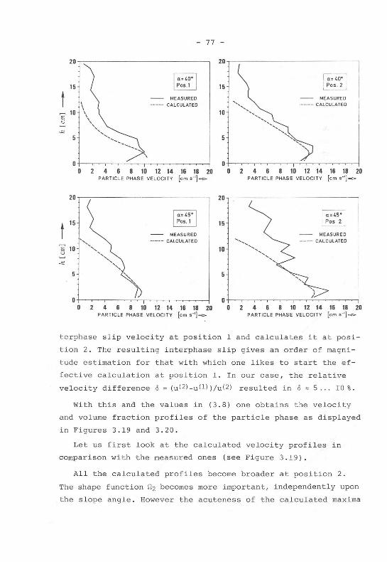
t 5

..s::

- 77 -

20 20

l [;1] la= 4a·-15 1 15 ~

I MEASURED MEASURED

----- CALCULATED ----- CALCULATED I 10 10

i

0 0+-~--.--r--~or~-r--~--r-~

0 2 4 8 10 12 14 16 18 20 0 4 10 12 14 16 18 20 PARTICLE PHASE VELOCITY (cm s·']-<> PARTICLE PHASE VELOCITY (cm s·']-<>

20 .-~-------------------------~ 20 .---------------------------~

~ ~

MEASURED

----- CALCUL ATED

15

10

a= 45• Pos 2

MEASURED

Ot--r-.--r-~~~~~~~~

4 10 12 14 16 18 20 0 2 4 6 10 12 14 16 18 20 PARTICLE PHASE VELOCITY (cm s·']-<> PARTICLE PHASE VELOCITY (cm s·']-<>

terphase slip velocity at position 1 and calculates it at posi­

tion 2. The resulting interphase slip gives an order of magni­

tude estimation for that with which one likes to start the ef-

fective calculation at position 1. In our case, the relative

velocity difference 6 = (u(2)_u(l) )/u(2) resulted in 6 " 5 .. . IO %.

With this and the values in (3.8) one obtains the velocity

and vo lume fraction profiles of the particle phase as displayed

in Figures 3.19 and 3.20.

Let us first look at the calculated velocity profiles in

comparison with the neasured ones (see Figure 3.19).

All the calculated profiles become broader at position 2.

The shape function n2 becomes more important , independently upon

the slope angle. However the acuteness of the calculated maxima

- 78 -

is more due to >1 1 . The value of the maxima is modelled very

well by the Kantorovich calculation; therefore, also the quali­

tative behavior concerning deceleration and acceleration of the

flow is adequately reproduced. Above 35°, the velocity increa­

ses downstream, as it should. The discrepancy between calcula­

tion and measurement at position 2 is to a large extent due to

that already present at position 1. One can of course find

shape functions for which the calculation and the measurement

at position 1 agree better. But in this case the downstream

evolution in the numerical computations is less satisfactory.

Also the agreement of the upper surface of the laboratory ava­

lanche is not as bad as it might seem from Figure 3.19. It must

t E <.J

.s::

t 5

.s::

Figure 3.20 Measured and calculate d particle phase volume fraction profiles.

20 .. -------------------------.

15 ~ Pos. 1 15 ~ 2

MEASURED ~ MEASURED CALCULATED CALCULATED

10 10

5 5

0 1· 2· 3· 4· 5· 6· 7· 8·10·3 0 1· 2· 3· 4· 5· 6· 7· 8·10.3

PARTICLE PHASE VOLUME FRACTION-<> PART ICLE PHASE VOLUME FRACTION -<>

20 20

15 ~ 1 15 ~ 2

MEASURED '01--. MEASURED CALCULATED CALCULATED

10 10

5

1· 2· 3 · 4· 5· 6· 7· 8·10-· 1· 2· 3· 4· 5· 6· 7· 8·10.3

PARTICLE PHASE VOLUME FRACTION-<> PARTICLE PHASE VOLUME FRACTION -<>

cont. _____.

- 79 -

20 20

15 ~ 1 15 ~ 2

t MEASURED ~ MEASURED

CALCU LATED CALCULATED ~ 10 10 E; C)

~

0~~~~~~~--~~--~~

5· 6· 7· 8·10.3 0 1· 2· 3· 4 · 5· 6· 7· 8·10·3

t

PARTICLE PHASE VOLUME FRACTION -<>

20 ~--------------------------~

15

1·

~ ~

2· 3· 4· 5· 6· PARTICLE PHASE VOLUME FRACTION-<>

15

10

1·

PARTICLE PHASE VOLUME FRACTION-<>

2· 3· 4·

~ ~

MEASURED CALCULATED

5· 6· PARTIC LE PHASE VOLUME FRACTION -<>

be kept in mind that above h = 12 cm the volume fraction of the

particle phase is so low, that one can consider it to be a re­

gion of pure water. The velocities in the uppermost regions are

velocities of isolated single polystyrene particles. That is why

the relative fluctuations there are larger than within the la­

boratory avalanche.

The initial (upstream) vol ume fraction profile of the par­

ticle phase was chosen to be the same for all slope angles, even

though the accuracy of this procedure is not very good. Compari­

son is however facilitated in this way. More than a qualitative

agreement is not to be expected in view of the simple shape

functions (see Figure 3.18). More important than the reproduc­

tion of the initial profiles is their change as they evolve

downstream. In this regard the numerical model agrees satisfac -

- 80 -

torily with the experimental data. The model exhibits the same

slope angle dependence. On a = 30° the particle phase volume

fraction at the very bottom increases in the downstream direc­

tion, on a= 35° it remains constant and on a= 40°, 450 it dimi­

nishes, i . e . particles are lifted upwards .

These results prove the workability of the theoretical model

as described in chapter 2, all physically relevant processes

and mechanisms seem to be included . Entrainmen t is of minor im­

portance, once the turbulent mixture is developed (see also

chapter 4). Although solutions with growing or diminishing flow

height may be found with the Kantorovich technique , their velo­

city profiles differ only marginally (in the order of 1 %) from

those with vanishing entrainment.

With the proven physical reliability of the numerical model,

we shall now look at so l utions which can not be tested against

laboratory data,and we shall study the effect of parameter va­

riation (as long as the parameters lie in a range where the

computer program converges).

All calcul at i ons were made with the initial condi tion

Ufluid phase < Uparticle phase and with a linear functiona l depen­

dence of the interphase friction upon the relative ve l ocity

(uparticle phase - Ufluid phase ). Variation of the model parameter

CFric/T indicated that CFric/T 2: 300 corresponds to a lmost a no­

slip condition. An exampl e of the computational results is

shown in Figure 3.21. The calculation at position 1 is started

with a significant relative ve l ocity between fluid phase and

particle phase. After 0.5 m downstream, this slip velocity va ­

nishes. The fluid phase has been accelerated, the particle

phase decelerated . It is also poss ible that both phases dece­

lerate, as is displayed in Figure 3 . 22 with CFric/T = 3 . The in­

terphase slip r educes from position 1 to position 2 , where it

is still 10% of the phase velocities.

The effect of the variat ion of CFric/T with a ll other pa r a ­

meters fixed may be seen in Figure 3.23.

t '=' 10 5

5

FLUID PHASE PARTICLE PHASE

- 81 -

OT--r--.-~~--.-~--~----~~ 0 2 4 6 8 10 12 14 16 18 20

DOWNSLOPE VELOCITY (cm s-')-<> 0 2

FLUID PHASE PARTICLE PHASE

4 6 8 10 12 14 16 18 20 DOWNSLOPE VELOCITY (cm s-')-<>

Figure 3.21 Fluid phase and particle phase velocit i es for a quasi-no-slip condition for the relative velocity.

20

(5 ~10 FLUID PHASE <:.J

PARTICLE PHASE ~

0+-~--.--r--~-,~~~~--~~

0 2 4 6 8 10 12 14 16 18 20 DOWNSLOPE VELOCITY (cm s-')-<>

20

15

10

5

2 4 6 10 12 14 DOWNSLOPE VELOCITY

16 18 20 (cm s-']-<>

Figure 3.22 Fluid phase and particle phase velocities for mo­derate interphase friction.

4 8 10 12 14 16 18 20 PARTICLE PHASE VE LOCITY (cm s-')-<>

Figure 3.23

Var i at ion of the interphase fric­t ion constant CFric/T.

- 82 -

The change of Crric/1 changes the particle phase velocity

profile only quantitatively, its shape remains essentially the

same. Unfortunately, the numerical scheme is very sensitive to

changes of Crric/T, if the shape functions are kept the same,

so the range of Crric/1-values for which convergence is obtai­

ned, is narrow. If the interphase friction is weaker (Crric/1 =

1.5), the particle phase decelerates less than for a larger

fr iction (CFric/1 = 6). This is not surprising, as the interphase

friction causes a continuous loss of momentum for the particle

phase, unless the fluid phase is faster, which was assumed not

to be the case in the calculations.

The success in reproducing the experimental results by the

Kantorovich-model is to a great extent due to a sophisticated

choice of the shape functions. They are not given algebraical­

ly, but only numerically. For many other sets of shape func­

tions, the agreement with the experiments was worse, or the

numerical method did not even converge. The next step would

now be to extend the model to N = 3, 4, 5 etc., thus to tackle

a quantitative mode ling . In any case the extension of the

Kantorovich technique looks more promising than a refinement

of the FD-mode!.

- 83 -

4. The transition flow/powder snow avalanche

4.1 Suggested transition mechanism

It is generally agreed upon that powder snow avalanches de­

velop from flow avalanches , but the mechanism, how the transi­

tion from one flow regime to the other takes place is not

known to date.

Because air plays a negligible role in the dynamics of flow

avalanches, but is important in the evolution process of pow­

der snow avalanches, one may speculate that it may also be sig­

nificant in the transition mechanism. In the flow avalanche re­

gime the volume fraction of the air is moderate ( - 70- 90 %); thus

its mass is small and consequently so is its dynamic role. The

volume fraction of the snow, on the other hand, is relatively

large. By contrast, in a powder snow avalanche the volume frac­

tion of the air is large -much larger than that of the snow­

and so the air must play a dynamic role, and the volume frac ­

tion of the snow is small. This chanqe in the volume (and mass)

ratio of air and snow is achieved by entluLi.rtmen.t of air through

the free upper surface of the avalanche. We thus conjecture

that entrainment is chiefly responsible for the transition

"flow avalanche to powder snow avalanche".

The flow avalanche limit can reasonably be treated as a

shear flow of granules whose momentum is transferred by binary

collisions. The continuum theory, that is based on the stati­

stical mechanics is known and given to various degrees of com­

plexity by Savage & Jeffreys (1981), Jenkins & Savage (1983)

and Lun et al. (1984). Scheiwiller & Hutter (1982) give a re­

view in the context of avalanche modelling. In order that air

can play a role for the transition mechanism this simple one­

component model must be extended to a two component mixture

of granules and air, in which the snow_phase is treated as a

continuum of small particles bouncing against each other,

whereas the air is regarded as a linear viscous fluid.

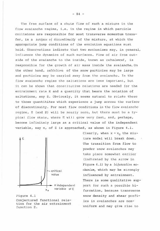
- 84 -

The free surface of a chute flow of such a mixture in the

flow avalanche regime, i.e. in the regime in which particle

collisions are responsible for most transverse momentum trans­

fer, is a ~Wq\ac.e of, d.U.,c.orttin!U;ty of the mixture, at which the

appropriate jump conditions of the evolution equations must

hold. Observations indicate that two mechanisms may, in general,

influence the dynamics of such surfaces. Flow of air from out­

side of the avalanche to the inside , known as en.tJr.IL{_nmeYLt:, is

responsible for the growth of air mass inside the avalanche. On

the other hand, ~~~atco~ of the snow particles may be large

and particles may be carried away from the avalanche. In the

flow avalanche regime the saltations are less important, but

it can be shown that constitutive relations are needed for the

entrainment rate E and a quantity that bears the notation of

saltations, say S. Obviously, it seems natural to relate these

to those quantitites which experience a jump across the surface

of discontinuity. For most f low conditions in the flow avalanche

regime, E (and S) will be nearly zero, but there must be a ty­

pical flow state, where E will grow very fast, and, perhaps,

become infinitely large as a critical value of the independent

variable, say x , of E is approached, as shown in Figure 4.1.

E

Figure 4.1

critical value

X independent variable of E

Conjectured functional rela­tion for the air entrainment function E .

Clearly, when x + x0 the mi x ­

ture model will break down.

The transition from flow to

powder snow avalanches may

take place somewhat earlier

(indicated by the arrow in

Figure 4 .1) by a b-l6uJtc.a.ti.on me­

c.ha~m, which may be strongly

influenced by entrainment.

There is some qualitative sup­

port for such a oossible bi­

furcation , because transverse

snow density and shear profi­

les in avalanches are non­

uniform and may give rise to

- 85 -

instabilities akin to the Kelvin-Helmholtz or Taylor-Goldstein

instabilities.

In what follows we shall first present the two-phase flow

equations which are thought to be appropriate for flow avalan­

ches. The model for the air is rough, because its role may be

important for the transition only. Emphasis will be on the

boundary conditions at the free surface and on phenomenologi­

cal relations defined for fields on such surfaces.

4.2 Theoretical formulation

The two-phase flow equations for a flow avalanche are estab­

lished under the assumption that

Snow is an assemblage of rigid, tacky particles, which , under rapid shear, experience binary collisions,

air is a linearly viscous fluid ,

both , snow and air are incompressible.

The latter of these assumptions does not say that the density

of the avalanche could not vary with position; it simply varies

according to the local proportions of air and snow present.

4.2 .1 Balance laws

The genera l balance laws for mass and momentum read (see

section 2. 3. 1) . d P V + n • ( pV V ) at V V 0 (4 .1)

(4. 2)

Obviously ( 2. 4), ( 2. 6) and ( 2 . 8) hold also for the two-phase 6tow avalanche.

4.2.2 Mean fields and fluctuations

Because our interest is only in the mean motion, balance

equation for the mean fields are derived (as in section 2.3.2):

ac v --at + V. (cv ~v ) = 0' ( 4. 3)

(4. 4)

- 86 -

where (4. 5)

(4. 6)

In the air K(l) is essentially the Reynolds stre ss tensor, in

the particle phase K( 2) accounts f or the momentum f l u x due to

co llisions . Additional re l ationships for Kv must now be estab­

lished. To this end, consider

~V® {momentum equation} ,

yielding (in component notation)

~c1' KY j v v v v at + (c Kij V9_ + Qij 9- ), 9,

( 4. 7)

(y~£ v~ ,j + Yj9, v~ . il + r~j + M~j

where V V V V

Kij Kji , Qij lt Qj i 9, , (4. 8)

V ' V' V' V '

rv . rv V V mi Vj + mj Vi = , Mij = Mji -

1) J 1 Pv are second and third order correlation tensors. (4.7) is an

evolution equat i on for ~v if only constitutive relation for Qv,

~v , £v are established.

A theory using (4.7) is too complex to have a realistic

chance to be amenable to explicit solutions for even the mos t

simple physical situations . For the particle and the air phase

two different procedures of simplification will thus be follo­

wed.

For the particle phase we assume that the fluctuation stress

is isotropic (a pressure, as in a ren l gas), so that

0. 1 (4. 9)

Contraction of (4 .7 ) thus y i e l ds

3 a c(2)e 3 q( 2) -2 -~-t-- + 11 · (-c ( 2 ) 0 v(2) + --- )

a - 2 - p (2)

G (2) N(2) tr (D= (Z) ·y( 2l) + -- + --

p(2) p(2)

(4.10)

*) tr(~) :: llii

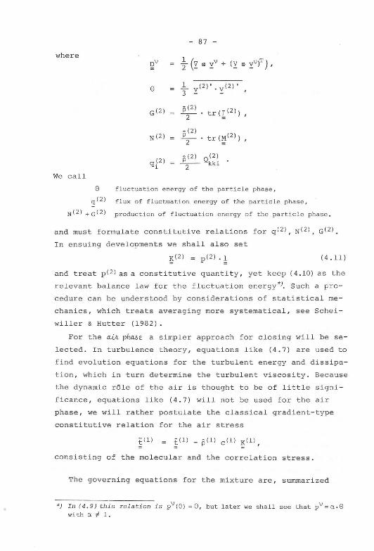
where

We call

0

q<2) 1

1 3

- 87 -

-p (2) -2- tr(~(2))

P- (2) -2- tr <;:;(2))

p (2) Q(2) -2-- kki

0 fluctuation energy of the particle phase ,

q< 2 l flux of fluctuation energy of the particle phase ,

N(2) +G(2) production of fluctuation energy of the particle phase .

and must formulate constitutive relations for q< 2l, N< 2l, G< 2l.

In ensuing develo9ments we shall also set

(4 .11)

and treat p(2) as a constitutive quantity, yet keep (4.10) as the

relevant balance law for the fluctuation energy*!. Such a fro­

cedure can be understood by considerations of statistical me­

chanics, which treats averaging more systematical, see Schei­

willer & Hutter (1982).

For the w phMe a simpler approach for closing will be se­

lected. In turbulence theory, equations like (4.7) are used to

find evolution equations for the turbulent energy and dissipa­

tion, which in turn determine the turbulent viscosity. Because

the dynamic role of the air is thought to be of little signi ­

ficance, equations like (4 . 7) will not be used for the air

phase, we will rather postulate the classical gradient-type

constitutive relation for the air stress

t(l) §<ll - ii(l) c<ll ~(1),

consisting of the molecular and the correlation stress.

The governing equations for the mixture are, summarized

*) In (4 .9) this relation is pv(8) =0 , but later we shall see that pv=CX · 0 with ex cl 1.

- 88 -

il c< 2l 1) - -- + V· (l-c< 2l)y< = 0, at

( l-c<2l)[ay<1l + v<1>.vv<1J] = V_·y<1l + (l-c<2l)g- !!)(2) a t - - - - ii<lJ'

+ _1_ t(1) fi (1)

t (1) f. (1) _ ii (1) ( l-c< 2J) ~ (1)

[a v<2l

(2) ---c a t

2_ (2) [a0 + v(2)· V_ 0lj 2 c at

N(2) + --

1)(2)

-c<2J p< 2i 1 + _l_ ) -c< 2l p 1 + t_(2) -J p <2l L = =

where we have used t = g, c< 2l = 1-c(l), ~(l) = -~(2).

(4 .12)

(4.13)

In (4.12) and (4.13) ~(1), p, c<2l, ~(2), 0 are regarded as ba­

sic fields (9 variables and 9 equations). Constitutive rela­

tions must be postulated for §<ll, §<2l, q(2), G(2), N( 2), m<2l.

4. 2 . 3 Constitutive relations

Two limits of (4.12) and (4.13) are of special interest.

When the air and particle phase are separate, (4.12) and (4.13)

uncouple, because !!1(2) = Q but only (4.12) is then meaningful.

On the other hand in a one-phase model for the particles one

has !!1(2) = Q, N = 0 and p = 0. In this limiting case the consti­

tutive quantities of the particle phase listed above have been

determined (incorporating various complexities) by explicitly

evaluating the relevant collision integrals. In such evalua­

tions flux terms arise which are either due to particle colli-

- 89 -

sions or else transport on the mean motion. In a dense agglo­

merate collisions are frequent and transport from collision to

collision, responsible for diffusion, is small. This may justi­

fy the neglect of the diffusive transport in the statistical

theory. In the presence of air, the drag exerted by the air on

the particles can only be effective between collisions and this

contribution has just been made plausible to be negligible. We

may thus use the constitutive relations, derived by J e nkins &

Savage (1983), who ignore the diffusive terms and add drag

contributions in a gross fashion. These constitutive relations

are

f. (2)

K(EJ ,c( 2l) _2_ p (2) (c(2) )2 a (l+e) g (c(2)) re 17! 0

I1T

q(2) - K{E) ,c( 2)) ~EJ 1

val id for rigid spheres.

In these relations the new symbols are

a Diameter of spheres

e Coefficient of restitution 0 . 8 - 1.0

a Free parameter arising in the statistical theory, assumed here to be constant = 1/ITT,

(4.14)

and g 0 is the radial binary correlation function at collision.

1 3c(2l go(c(2l) = --- +

l-c( 2) 2(1-c(2l) (4 .15)

valid for c(2) :S 0. 7, which is realistic.

Hutter, Szidarovszky & Yakowitz (1986) have shown that a gra­

nular model that excludes the explicit appearance of air and

uses the constitutive relations (4.14) does not permit solu­

tions of steady shear flow when a surface drag resistance is

- 90 -

incorporated. They prove that the particle stress i(2) must be

complemented by a term which is proportional to the dyadic pro­

duct of the particle concentration gradient. Thus

i( Z) = i (2 ) (eq , (4.14)) - A· (~c(2)) 0 (~ c<2l) (4.16)

(\ = phenomenolog ical constant, assumed small > 0

in which the first term on the RHS is given in (4.14) 1 and

where A is a positive constant. Such a term also arises in mo­

dels of suspension flows of particles in fluids, see i.e. Mills

(1966) , Craine (1971), Garg & Pritchett (1975) and has arisen

in early theories of granular fluids (see Nunziato et al. ( 1980)) .•

Alternatively, one may change the e xpressions (4.14) by incor­

porating terms which remove the mentioned difficulties.

We still need phenomenological relationships for the momen­

tum production~ and the energy production N( 2). Drag should

vanish for plug flow (c = Cmax::: 0. 74), but otherwise reflect a

dependence on concentration and velocity,

(4 .17a)

A = drag coefficient

in which A may still depend on the magnitude of the difference

velocity lly<ll _y <2> 11 and possible other variables. Whether this

is so or not depends on the fact whether the boundary layer

flow around the particle is laminar or turbulent. In view of

the fact that the air will play a secondary role, A will be as­

sumed constant. With (4.17a) and the definition of N(2), it is

easy to show (by ignoring fluctuations of c<2) as above) that

(4.17b)

Thus N(2) is composed of a production/annihilation term and a

strict annihilation term, whereby the first of these is formed

by the air-particle correlation tensor. It is reasonable to re­

late this mixed correlation tensor to the "diffusional kinetic

energy" (4.17c)

q, = constant,

- 91 -

For <jl> O the RHS of (4.17c) is negative and N(2) acts as a

strict energy sink . One could also argue that y<2l' is collinear

to v<ll' implying y<ll' · y(2)' is proportional to 8. This choice

would simply correspond to (4 .l7b,c) with <P = 0 and a different

coefficient A. We prefer (4 . 17c) with <P t 0.

We still must establish a constitutive relation for the to­

tal stress of the air phase. We choose

~(l) = 2~~(l) --}~· tr (~(ll) ~

~ = viscosity of the air phase in the mixture , assumed constant.

( 4 .18)

The equation corresponds to a classical flux-gradient clo­

sure. With this , the system (4 . 12)-(4.18) is closed. Solution

for the i ndependent field variables is possible in principle,

but requires knowledge of boundary conditions. It should also

be mentioned that all above constitutive quantities are objec­

tive isotropi c relations. Specifically, the particular stress

t ensors t_ (2l, t<ll are symmetric . In mixture theory this is no

necessarity, but the selection of symmetry does not violate

general principles either.

4.2.4 Boundary conditions at the free surface

The free surface of an avalanche is defined as that surface

which separates the snow- air mixture from the air. This is a

<~Wt6ac.e co6 cU.oc.orrt-i.J'!UAXlf at which many field va riab le s may expe­

rience a finite jump. Derivation of boundary conditions thus

amounts to formu l ating the component jump conditions of mass

and momentum. Furthermore kinematic conditions must hold. For

X

simplicity only plane flow

will be considered, see

Figure 4.2.

Figure 4 . 2

The surface of an avalanche as surface of discontinuity . The air - side will always be the (;:; - side.

- 92 -

Let F = z- Zs (x, t) = 0 be the equation of the singular sur-

face. Then J z 5 1/ az ~ = (- ~x , 1)/ ~l + ( ax

5)2 (4.19a)

is its outer unit vector and

u - w s s 0 '

( u5 , W5 ) = vector of surface velocity,

(4 .l9b)

its evolut ion equation. (4.19b) is called kinematic (surface)

condition.

Observations of suspended particles in steady turbulent

flows near walls indicate that the upper surface is fluctuat ­

ing . This suggests decompositions Zs = Zs + z~, Vs = Vs+ v~ and

l eads to the average surface equation

d Z~ u~ = - s

where S can be interpreted as an accumulation/ablation contri­

bution. The equat i on says that the average surface does not

follow the average velocity , but a velocity given by (u;,w;)

(us,Ws-Sl. In terms of this velocity, (4.19b) is recovered (for

Zs and y; ). This equation will be used in the sequel, but we

will omit the overbar and the asterisk.

On a singularity surface, conservation of mass implies

( 4. 20)

Here, [ljJ ]: = ljJ+- ljJ-, in which the indices± denote the limit va ­

lues of the indexed quantity as the singul arity s urface is ap­

proached from the (+) and G- side, respectively. In the follow ­

ing no index will always mean the G - side.

For lhe particle phase we require p ( 2)+ = 0, so ( 4. 20) implies

v( 2 >-e = y5·~, but without loss of generality we may set v(2)=

Ys : 6otr. the pa!!.Uc..te6 the <1-i.ngu.!a.tr. <~u.tr.6ac.e ~ matetr.-<.a.t,

a z 5 d Z5 + v( 2) _v(2) = 0, at z = z 5 (x,t). dt dX X Z

( 4. 21)

- 93 -

Consider now the air phase. Equation (4.20) may then be

written as [c<ll(~(l)-~(2)).~] =0, or

-E, (4. 22)

E ~ entrainment ,

in which c<ll+ = 1 has been used, The e.n.Vr.a..{.rtme.n.t 6unc.tion is the

crucial quantity of this theory. We therefore emphasize that

its physical meaning is advective volume flux of air through

the singular surface. We presently regard it as a prescribed

quantity. Using (4.19a) in (4.22) and in the resulting equation

(4.21) the following second kinematic equation is obtained:

(4. 23)

Equations (4.21) and (4.23) together exploit the kinematic re­

lations and the jump conditions of mass.

Dry snow avalanches show frequently a thin layer of air

borne snow at the upper surface, of which the density is sub­

stantially smaller than within the flow avalanche. Outside wind

gusts occasionally carry this snow away into the air, and this

snow drift seems to increase with increasing saltation at the

surface. To account for the drift the right hand side of (4.21)

would have to be replaced by -D·(l+( dz 5 /ax)2 J112 where D plays

the role of a (negative) entrainment and would be related to

the atmospheric conditions. We shall ignore snow drift and

thus set D = 0.

b) Jump o6 momentum

The boundary conditions of tractions are obtained from the

jump conditions of momentum

( 4. 24)

For the snow phase, since p (2)+ = 0 and ~(2)- = ::s, this yields

[;!(2).~] = 0, or in view of (4.12) 4 and (4.19a)

[p<2l c<2l (_R_ +p<2ll -f,\2>] azs + E~il = -t~~l+ ~ + t~~t, p<2l x ax ax

(4. 25)

-(2) 3zs -(2) (2) (2) P (2) txz -;:;--X - tzz + P c (- + P )

0 p(2)

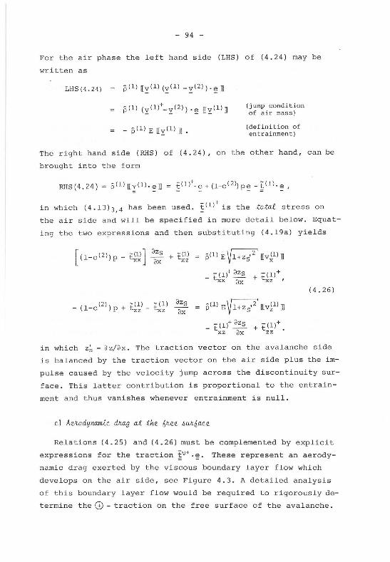
- 94 -

For the air phase the left hand side (LHS) of (4.24) may be

written as

LHS(4.24)

_ p(l) E [~(1)].

(jump condition of air mass)

(definition of entrainment)

The right hand side (RHS) of (4.24), on the other hand, can be

brought into the form

in which (4.13) 3 , 4 has been used. ~(l)+ is the tota.t stress on

the air side and will be specified in more detail below. Equat­

ing the two expressions and then substituting (4.19a) yields

azs ax

P(l) EVl+zs'2' [v~l)]

-( 1 / azs -( 1 )+ - txx :h{ + txz '

(4.26)

in which z~ = a z/3x. The traction vector on the avalanche side

is balanced by the traction vector on the air side plus the im­

pulse caused by the velocity jump across the discontinuity sur­

face. This latter contribution is proportional to the entrain­

ment and thus vanishes whenever entrainment is null.

Relations (4.25) and (4.26) must be complemented by explicit

expressions for the traction §v+.~. These represent an aerody­

namic drag exerted by the viscous boundary layer flow which

develops on the air side, see Figure 4.3. A detailed analysis

of this boundary layer flow would be required to rigorously de­

termine the G.J - traction on the free surface of the avalanche.

- 95 -

We are less ambitious and take the boundary layer mechanism

into account in a gross fashion by postulating that the shear

traction can be related to the tangential velocity and that the

total normal stress of the air on the surface equals -patm. Con­

sequently,

1::

at <:: = z5 (4.27)

V:= v(lj+ - v(l)+ (oo).

air

0 avalanche

Figure 4.3

Atmospheric boundary layer flow introduced by the ava-lanche.

The first of these is a nor­

malization condition that must

be imposed in order that the

atmospheric boundary layer

need not be analysed in grea­

ter detail. W i s a vector tan­

gential to the free surface

and V is the difference velo­

city of the air between the

surface and infinitely distant

from it. c<ll (.) is the dimen­

sior.less drag coefficient, pre­

scribed by a phenomenological

relation, and(.) expresses such

a dependence that will be ~ade

more explicit below. With the aid of (4.18) the relations (4.27)

l ead to

(4. 28)

- 96 -

By substituting these ex?ressions into (4.26) the final form

of the jump conditions of the air stress at the free surface

is obtained. Usual computations will be in terms of relative

stresses; this implies that we may assume patm =0. This will

henceforth be assumed.

In (4.25) we also introduce the part icle tractions on the

+" - side, even though p (2)+ = 0. The reason is that aerodynamic

drag will be exerted on both, the particle and the air phase,

and that on the particle phase is intuitively the larger of the

two. Using the same procedure as above one obtains

(4.29)

- ij(2> c< 2> <·l

I Vz-Vx zs] p,2 . lvz- ' l+zs ' l+zs2

in which c< 2> (·) is a new drag coefficient.

Several new variables have now entered through the boundary

condition of the free surface. These are

(4.30)

but of these five, entrainment and the latter two are interre­

lated. To see this, the defining equation of the entrainment,

(4.22), and relation (4.19a) are used to deduce the fol lowing

relation:

[v(l)]- [v(l)] dZs = (v( 2) _V(l))- (v(2)_V(l ) ) azs - E \~ z X dX z z X X dX V 1 + z s- . (4.31)

Thus, given [v~1 l] and the entrainment and solving for the ava­

lanche flow determines [v~ ll]. Further, when E = 0, then

(v<l)-_~(2))·§ 0, and combining (4.21) and (4.23) also

(v <l) - -v<2)) · e 0. It follows that - - -

- 97 -

[:::(1)] • ~ = 0' when E = 0.

In the absence of entrainment there can be no jump of the

air velocity normal to the free surface. This suggests, and

corroboration can easily be provided, that a coordinate inva­

riant form of (4.31) is

(4. 32)

We now conclude that the tangential component of the air­

velocity jump [:::<ll " ~], is still free ( " is the symbol for the

cross product). However, since the air is treated as a viscous

fluid, both within and outside the avalanche, the no-slip con­

dition must apply, which can be e xpressed as

0 , or az

[v(l)] + [v(l)] --5

z z ax 0. (4. 33)

The appropriate jump condition on a singularity surface for

the balance law of the fluctuation energy for the particles (4.10)

is not clear but when radiation of fluctuation energy into the

atmosphere is ignored we have

In plane Cartesian coordinates this relation reads

8z5 q~2l_q~2) ax- = o.

(4 . 34)

(4.35)

This no-flux condi tion is an i dealization which may have to be

altered in later , more careful analyses. When the aerodynamic

drag on the atmospheric side is taken into account, this drag

effectively acts as a sink of fluctuation energy of the parti­

cles . Thus, there should be a non-vanishing flux of fluctuation

energy through the free surface, expressibl e as g< 2 J+.~ * 0.

6! Con~ono on ~et~ eone~~on

I ntuit i vely one might think that the above boundary condi­

tions suffice. This is however only so, when A = 0. I n case the

stress tensor A c< 2l c< 2l is present one add i tional boundary con-, 1. , J

- 98 -

dition involving the particle concentration is needed. We do

not clearly understand what boundary condition would be appro­

priate and whether it should be formulated at the free surface

or the base. Here we propose a relation at the free surface,

(l-c<2l) = xe, at z = z 5 (4.36)

with constant x and thus set the volume fraction of air pro­

portional to the saltation level. Nunziato et al. (1980) request

dc< 2l/dz = 0 instead of (4.36), but obtain particle distribution

functions which poorly match observations. Equation (4.36) seems

to be heuristically correct.

4.2.5 Boundary conditions at the base

Several alternatives are possible in an avalanche. The snow

may adhere to the bed for all times or a sliding plane may de­

velop. We shall confine attention to the no-slip condition for

snow and air, leaving more genera l conditions to a future study.

This fixes the velocities , but does not yet determine which

boundary conditions should be imposed for the fluctuation ener ­

gy. Hutter, Szidarovszky & Yakowitz (1984) have shown that the

simultaneous imposition of zero velocity and zero fluctuation

energy at the basal surface offers difficulties in the general

solution procedure of simple shear flow of a granular material

following the Jenkins-Savage theory. In fact, without the

stress contribution Ac<?l c<:!'l see (4.16) in the particle , 1. , J , ,

stress tensor, non-existence of solutions of steady chute flow

can be proven, if zero velocity and zero fluctuation energy is

imposed at the base. Alternatively, when A ~ 0 the solution

would be singular. Scrutiny shows that the same difficulties

would also arise here. We will thus impose the boundary con­

ditions

o·e+ ~ an 0, at z = z8 , (4. 3 7)

with a coefficient o that may, in general, also depend on other

variables but will be assumed constant for our purposes here;

o = 0 corresponds to vanishing flux of fluctuation energy through

- 99 -

the surface. o = oo is the expression of zero fluctuation energy;

it causes the singular behaviour mentioned above. There are no

more boundary conditions than (4.37), if the base is regarded

as permanent.

4.2 . 6 Remarks on solvability

The field equations (4.2)-(4.18) may be regarded as a set of

differential equations for c(2), p, 8, ~(1) and ~(2). By substitut­

ing the constitutive relations into the balance laws and by con­

sidering plane flow, seven part i al differential equations are

obtained for the seven unknowns, so integration is possible,

at least in principle.

With the kinematic conditions (4.21), (4.23) and the traction

conditions (4.25), (4.26) and (4.28), (4.29) z 5 ,E , C(l),C(2),

l[ v(l)] enter as new quantities, but [~(1)] can be written in

terms of the former using (4 . 32) and (4.33). Expressing E, c(l>

and c<2> through phenomenological equations in terms of other

quantitites z5 remains as the only other field variable of the

theory. Scrutiny of the field equations shows that the kinema­

tic and dynamic boundary conditions suffice to determine all

"integration constants" and the function zs(x,t). Explicit

proof for this will be provided in the following sections.

4.2.7 Constitutive relat i ons for entrain­ment and aerodynamic drag

Observations on real avalanches and also on laboratory ex­

periments suggest that the transition from the flow avalanche

to the powder snow avalanche is a sudden event. In other words,

E is small for flow avalanches but suddenly becomes large when

the transition to powder snow avalanches takes place. Assuming,

moreover , that E can only depend on local variables, that is

properties on the free surface, and denoting such a variable by

x,a qualitative graph of E(x) must look as shown in Figure 4.4.

For small va lues of x entrainment nearly vanishe s. Such condi-

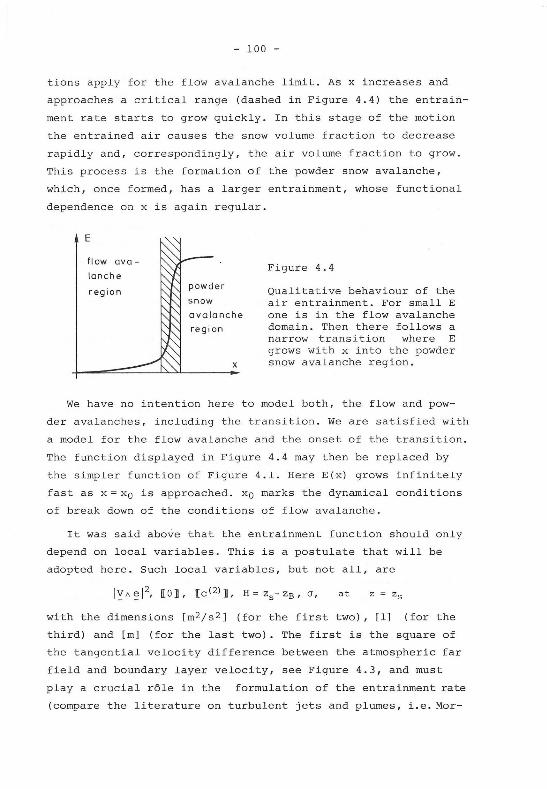
- lOO -

tions apply for the flow avalanche limit. As x increases and

approaches a critical range (dashed in Figure 4.4) the entrain­

ment rate starts to grow quickly. In this stage of the motion

the entrained air causes the snow volume fraction to decrease

rapidly and, correspondingly, the air volume fraction to grow.

This process is the formation of the powder snow avalanche,

which, once formed, has a larger entrainment, whose functional

dependence on x is again regular.

E

flow

lonche

region

Figure 4 .4

Qualitative behaviour of the air entrainment. For small E one is in the flow avalanche domain. Then the re follows a narrow transition where E grows with x into the powder

x snow avalanche region . +-~~~~~------

We have no intention here to model both, the flow and pow­

der avalanches, including the transition. We are satisfied with

a model for the flow avalanche and the onset of the transition.

The function displayed in Figure 4.4 may then be replaced by

the simpler function of Figure 4.1. Here E(x) grows infinitely

fast as x = x 0 is approached. x 0 marks the dynamical conditions

of break down of the conditions of flow avalanche.

It was said above that the entrainment function should only

depend on local variables. This is a postulate that will be

adopted here. Such local variables, but not all, are

at

with the dimensions [m2js2] (for the first two), [l] (for the

third) and [m] (for the last two). The first is the square of

the tangential velocity difference between the atmospheric far

field and boundary layer ve locity, see Figure 4.3, and must

play a crucial role in the formulation of the entrainment rate

(compare the literature on turbulent jets and plumes, i.e. Mor -

- 101 -

ton et al. (1 956)). The above permits construct i on of the di­

mensionless quantit i es

RiE gc(2) H

Ri1 gc<2l 0

= I :! " ~ 1

2 [8]

I~"~ 12 (4. 38)

c<2l = c<2l- I [ c < 2 l] I, a = a/H, b [8]

RiE and Rii may be interpreted as an external and internal

.<_rtteJt6a.ua.e. R-<-c.hMd6ort rtwnbeJt, a is the inverse of the number of

particles per height, and b is the ratio of the tangential ki­

netic energy to the fluctuation energy. In the definition of

RiE the analogy with the classical Richardson number is evident

except for the var i ab l e H~, but a length scale must enter. No­

tice that Rii only depends on "particle variables", while RiE

is formed with quant i t i es, which are peculiar to the particle

phase and the air phase. Finally, we mention that the defini­

tions RiE and Rii are only meaningful as long as the jumps

[c<2l] and [ 8] do not vanish or become infinitely large. This

is tacitly assumed here and requires regularity of the differen­

tial equations and boundary conditions at the free surface.

It is now postulated that E is dimensionally homogeneous:

E = E(RiE, Rir, c<2l - , a, b) but the dependenc i es on RiE, c<2l, a , b

are thought less significant in comparison to that on RiE = Ri.

S i nce, moreover, E i s expected to grow with growing I'!" <:12

and to decrease with growing [c<2l] and H, we set E = E(l/Ri).

For high shear rates, when saltations of the particles are

large and frequent, a relation of the form E = E (RiE, Ri 1 ) may

be necessary but we will not use i t here.

*) The classical Richardson number is defined as

3p 1 3;p

g 13vJ2'

3zl

where 3p/3z is the vertical dens i ty gradient and v the horizontal ve­loc i ty in a vertically stratified fluid. RiCl needs no length scale as it is included in the derivatives.

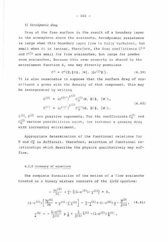
- 102 -

b) Avr.odyna.nLi.e dltag

Drag at the free surface is the result of a boundary layer

in the atmosphere above the avalanche. Aerodynamic resistance

is large whe n this boundary laye r flow is fully turbulent, but

small when it is laminar. Therefore, the drag coefficients c(l )

and C(2 ) are small for flow ava l anches, but large for powder

snow ava l anches. Because this same oroperty i s shared by the

entrainment function E, one may directly postulate

( 4. 39)

It i s also reasonable to suppose that the surface drag of con­

st i tuent a grows with the de nsity o f that component. This may

be incorporated by writing

c( 2l s ' 2l

(c( 2 l -l c~2 l(E , [ 0 ], IWil,

B(l) (c(ll-) C/} l (E, [ O], lW I) .

( 4. 40)

S (ll, 6(2l are positive exponents. For the coefficients ci}l and

c62l various possibil i t i es exist, for instance a growing drag

with increasing entrainment.

Appropriate determination of the functional relations for

E and cg is difficul t. Therefore, sele ction of functional re­

lationships which describe the physics qualitatively may suf­

fice.

4.2 . 8 Gloss ary of e quations

The complete formulation of the motion of a flow avalanche

treated as a binary mixture consists of the Metd equ.a.tioYL6:

(2) -~+ V · ((l-c( 2l)·v(ll) = 0, at - -

[ av(l ) J m (2)

(l-c' 2l) --- +v(ll. v v(ll = V· y(ll+(l-c(2))g --7--, at - -- - = - p(ll (4. 41)

l- c(2) 1 - --;s<ll P ~ + p( l) t(l) -(l-c( 2)) ~(1)

- 103 -

a c< 2 > -at + ~ 0 ( ~ ( 2) :::: ( 2) } 0 ,

[av<2> J m< 2> c(2) ___ + v_<2) o_'Jv_<2> = IJ_oy(2) + c(2) g + __ _ at - p(2)

3 [ae l 1 G< 2> N< 2

> - c {2) ~ + v ( 2) 0 'J 0 I = - - 'J 0 q ( 2) + tr ( =D=y} + -P ( 2) + 2 at - - " i)<2>- - fi<2>

q(2)

y=(2) = -c <2> p(2) __ 1 + _1_ [-c<2) P 1 + E<2>] , p(2) = =

211 !?(l)_ ~ 11 tr(D(l) ~,

---'--~~-'--11-- K(0,c( 2)} /8 1 a c<2> fi(2)

l-e

2a 2

1

l-c<2>

(4 0 42}

(4 0 43}

(4 0 44}

On the free surface, the interphase between avalanche and

air, the following bou.rtdaJty c.oncl..i..tioYL6 must be fulfilled*!:

*) All quanti ties with no superscripts G) must be evaluated on the 8 -side of the surface z = zs(x,t)o

- 104 -

Kinematic conditions :

~ + ~ vx(2) -vz(2) 0, at ax ( 4. 45)

(1) I ~7S ~ v(l) - v(l)] = E c L at + ax x z

Dynamic conditions:

-(2) :l zs -(2) + P-(2) c(2)(...!:_ + p(2)) txz ax - tzz i3 (2)

( 4. 46)

( 2) - (l) _ t- (l) <lzs - (l-e ) P + tzz xz aJ{

0 ,

in which

V (4.47)

- 105 -

Consistency condition:

(4. 48) 0 •

Furthermore, constitutive equations for entrainment and aero ­

dynamic drag must be satisfied

E E (Ri),

(ca)Ba ea D

(a= 1,2)

cg ( [8], lwl, Ril ( 4. 49)

where g![c(2)]1 H

I'::':" !:: 12 Ri

The boundary conditions at the base z = z 8 (x) read

v<ll = 2' v(2) = 0

ae 7.~

ae

6·8 + ax az

0

~ B

(4.50)

and express the no-slip condition and an energy radiation con­

dition. These equations contain the following constant coeffi­

cients, which in an actual computation must be accordingly se­

lected:

a 1,

a diameter of spherical particles,

e coefficient of restitution 0.8- 1.0,

/..

A>o

drag coefficient for particle-air interaction force ,

coefficient of the particle stress contribution c~f)

. (1)' (2) ' coefficient describing the energy dissipation due to ci vi in terms of the diffusional energy ,

c<2)max S 0.74. Maximum particle volume fraction for identical spheres,

~ viscosity of air,

s<ll, 8(2) exponents arising in the law of aerodynamic drag,

X coefficients arising in the boundary condition at the free surface

6 coefficient arising in the boundary condition of energy at the base.

- 106 -

4.3 Discussion

Consider plane flow of an avalanche down an inclined chute.

Assume that the head is far distant so that attention can be

focussed on the tail, see Figure 4.5. Assume, moreover, that

the process is in the flow avalanche regime. Under these condi­

tions air plays a secondary

X

z

Figure 4.5

Illustrating the steady flow of a flow avalanche down an inclined plane.

role and entrainment at the

upper surface is small. In

the absence of air entrain-

Ment and under the assump ­

tion of steady snow and air

flux from a cross section

far upstream it is conceav­

able to assume that there

exists steady (tail) flow

which is independent of the

lonqitudinal variable x. In

other words, with no entrain­

ment, z 5 = H =constant and

with a;ax = 0 for all variab­

les integration of the governing equations may be possible.

For non-vanishing entrainment steady solutions may still exist,

but they are necessarily x-dependent because with progressing

x air mass is continuously added . Since entrainment is small

in the flow avalanche regime the growth of z = z 5 (x ) with x un­

der the same physical situation is likely to be small. This

fact may serve as motivation for the assumption that

all fields vary much more in a direction transverse to the main flow than they do parallel to it.

This suggests that I dljl/ax l/1 dljl/dz I « 1 for any field ljl. We call

this assumption the !>ha.Uow MWW appwW!a.Uon and the consequen­

ces that evolve :':rom its application may be explored.

The result will be that to lowest order the strictly paral­

l el sided slab with no entrainment can be analysed. Of course,

- 107 -

this requires that the avalanche process takes place in a re­

gime where the air entrainment is indeed small, see Figures

4.1 and 4.4.

The next step is the analysis of pure shear flow, assuming

an entrainment as in Figure 4 . 1 and letting x approach the

critical value x 0 to simulate the transition to the powder

snow avalanche regime.

The treatment of the flow avalanche as a mixture presumes

the knowledge to model it as a one- phase granular material

(see Hutter, Szidarovszky & Yakowitz, 1986). However, one is

faced there with enormous numerical problems (Hutter, Szidar­

ovszky & Yakowitz, personal communication). Once these are

overcome, the numerical model must be generalized to two pha­

ses. Only after this is done, the simulation of the transition

is possible. Therefore, numerical resul ts cannot be presented

yet. But the idea of this boundary condition induced instabi­

lity has to be pursued further.

- 1 08 -

5. Summary and concl usions

In this work we have first developed a theory for the dyna­

mics of powder - snow avalanches . They are treated, within the

framework of continuum physics , as mixtures of two phases, na ­

mely snow particles and air which are coupled by friction. This

yields a theory for a turbulent gravity- driven dispersed two ­

phase flow with a free surface. The latter is defined as the

surface where the volume fraction of the particle phase jumps

discontinuously to zero . It is material with regard to the par­

ticle phase, whereas fluid is entrained from outside. The equa­

tions are closed by a k - s - model for the turbulence and by a

linear relationship between interphase friction and the rela­

tive velocity of the particles and the fluid. The theory is

only applied to plane steady flow .

On the other hand the workability of laboratory simulation

of powder-snow avalanches was demonstrated. To this end, a

l arge basin and a chute were constructed. The laboratory ava ­

lanches consist of a mixture of polystyrene particles and water.

Methods of measuring the particle phase volume fractions and

velocities by an ultrasonic technique which was originally de ­

veloped for blood flow applications, was adapted for hydraulic

models. Boundary layer profiles of the particle phase velocities

and volume fractions were measured in the steady body of labora­

tory avalanches on a constant slope. Unfortunately, it was not

possible to measure the water velocity. However, th i s would be

important to prove experimentally the i nterphase slip velocity.

Efforts should now be focussed upon the performance of experi ­

ments on more complex conf i gurations (for instance on a vari­

able inclination) and exper i ments of transient parts of the

flow, especially the avalanche head. I n order to compare the

theory with the experiments, the govern i ng equations were sol ­

ved numerically by two different methods. The convent i onal FD­

model (PHOENICS) failed because of the l arge numerical diffusion .

On l y uniform velocity profiles cou l d be obtained . Th e Kantoro -

- 109 -

vich technique y i elds reasonable results, but it must be admit­

ted , that it profits very much from the experimental results

inasmuch as the measured profiles suggest the shape functions .

They must be chosen such that the initial condition can be ap­

proximated by combining t hem linearly. Success or failure of the

Kantorovich technique depend crucial l y upon their choice. They

must be physically suggestive and at the same time allow con­

vergence of the algorithm. Thus far , computations were made

with N= 2 only , hence the results have to be judged from aqua­

litative point of view rather than from a quantitative one . In

this regard the achieved agreement between computations and

experiments by adjusting the model parameters approximately is

satisfactory . We have thus gained a basic physical understand­

ing of the steady body of the laboratory avalanches (and to

some extent also of the powder - snow avalanches), since all the

relevant phys ical processes and mechanisms seem include d in the

model . The next task is now the improvement of the numerical

technique to obtain quantitative results. First the Kantorovich

technique may be extended toN= 3, 4, 5 etc. Such higher order

models can be made more objective by using an orthogonal system

of shape funct i ons, i.e. the first N functions of that system

(for exampl e of the Legendre polynomials). The need for a pri ­

ori - information from experiments could then be omitted. Fur­

thermore the theory has to be general ized to more realistic

configurations comprising complex topographies (like a curved

or discontinuous bottom) . Finally one should attempt transient

computations. But even if these genera lizations are not yet

numerically manageable, it is possib l e to scudy natura l confi ­

gurations through the laboratory simulation.

Both, theory and experiments are based on a two - phase con­

cept which permits extension to take into consideration also

the runcut zone with the sedimentation of the particles. The

Kantorovich technique is very efficient with respect to compu­

ter time if plane flow is assumed , because the emerging equa­

tions are ordinary different i al equat i ons.

- 11 0 -

In the last chapter a theoretical attempt is made for the

transition from the flow avalanche regime to the powder - snow

avalanche regime. This transition is mode1ed as an instabi l ity

induced by the boundary condition at the free surface. In a

critical f low state, expressed as a Richardson number crite­

rion, the entrainme nt is greatly enhanced. Beyond that, once

the turbulent mixture of the powder-snow avalanche regime has

developed, the e ntrainment again becomes a well-behaved func­

tional of the flow state. No numerica l results can be presen­

ted, however, because even the numerical model for a one-phase

granular flow (for the flow avalanche) is not yet fully estab­

lished.

- 111 -

ACKNOWLEDGEMENTS

This work was made possible by Prof. Dr. D. Vischer

who provided all facilities and equipment of the Labo­

ratory. He also served as referee for my dissertation.

His continuous support and generosity is gratefully

acknowledged.

I a;n very much indebted to my advisor and teacher

PD Dr. K. Hutter . With his scientific impetus he was

a motivating and patient guide.

Chrispin Bucher and Felix Hermann helped me in plan­

ning and constructing the experimental set-up. The re­

alization was possible only due to the skill of our

workshop staff.

I thank Prof. D.B. Spalding from Imperial College,

London and CHAM Ltd, London for making available to us

the computer code PHOENICS and Prof. Dr. M. Anliker

from the 'Biomedizinisches Institut' at ETH for lending

us the ultrasound equipment. I also had many fruitful

discussions with Prof. Dr. T.R.H. Davies from Canter­

bury, New Zealand and Dr. H. Gubler and Dr. B. Salm,

and in particular, with Prof. Dr. c. Jaccard from the

Swiss Federal Institute for snow and avalanche research

(SFISAR), who has also served on my thesis committee.

All these people's work is greatly appreciated .

I thank F. Langenegger for the excellent typing.

During this work, I was financially supported by the

SNF and the SFISAR.

REFERENCES

Anonymous

Beghin P.

Craine R.E.

Davies T.R.H.

El l ison T.H., Turner J.S.

- 112 -

1980. Signalverarbeitung in Ultraschall-Puls ­Dopplergeraten, Praktikumsanleitung. Institut fur Biomedizinische Technik der Universitat und der ETH Zurich.

1979. Etude des bouffees bidimensionnelles de densite en ecoulement sur pente avec applica­tion aux avalanches de neige poudreuse. These, Grenoble.

1971. Oscil l ations of a plate in binary mix­tures of incompressible Newtonian fluids. Int. J. of Engng . Sci., Vol. 9, pp. 1177-1192.

1979. The investigation of avalanche processes by l aboratory experiments; exploratory tests. Internal Report of the Laboratory of Hydrau­lics, Hydrology and Glaciology, ETH Zurich.

1 959. Turbulent entrainment in stratified flows. J. of F l uid Mech., Vol. 6, pp. 423-448.

Frost N., 1977. Handbook of Turbulence. Volume 1. Ple-Moulden T. H. (Ed. l num Press, New York .

GargS.K., Pritchett J.W.

Gubler H.U.

Gubler H. U. , Hiller M.

Heisenberg W.

Hopfinger E.J.

Hutter K., Sz idarovs zky F., Yakowitz S.

1975. Dynamics of gas-fluidized beds. J. Appl. Phys., Vol. 46, pp. 4493-4500.

1981. Messungen an Fliesslawinen. Interner Be­richt Nr . 600 des Eidg. Inst. fur Schnee- und Lawinenforschung (EISLF), Weissfluhjoch/Davos, Switzerland.

1984. The use of microwave FMCW radar in snow and avalanche research. Cold Reg. Sci. and Techn., Vol. 9, pp. 109-119.

1948. Zur statistischen Theorie der Turbulenz. z. flir Physik, Vol. 124, pp. 628-657.

1983. Snow avalanche motion and related phe­nomena. Ann. Rev. of Fluid Mech., Vol. 15, pp. 47-76.

1985. Wet-snow-flow avalanches treated as a plane steady shear flow of a cohesionless gra­nular material down an inclined plane (in pre­paration) .

Jansen R.H.J.

Jenkins J.T., Savage S.B.

Jones W.P., Launder B.E.

Kantorovich L.W., Krylov W.I.

Kolmogoroff A.

Launder B.E., Spalding D.B.

Lun C.K.K., Savage S.B., Jeffrey D.J., Chepurniy N.

Mellor M.

Middleton G.V.

Mills N.

Monin A.S., Yaglom A.M.

Morton B.R., Taylor G., Turner J.S.

Miiller I.

- 113 -

1978. The in situ measurement of sediment transport by means of ultrasonic scattering. Publ. No. 203 of the Delft Hydraulics Labora­tory, Netherlands.

1983. A theory for the rapid flow of iden­tical smooth, nearly elastic spherical par­ticles. J. of Fluid Mech., Vol. 130. pp. 187-202.

1972. The prediction of laminarization with a two-equation model of turbulence. Int. J. of Heat and Mass Transfer. Vol. 15, pp. 301-314.

1958. Approximate Methods of Higher Analysis. Interscience Publishers.

1941. The local structure of turbulence in incompressible viscous fluids for very large Reynolds numbers. Comptes rend. de l'Acad. des Sci. de l'URSS, Vol. 30, pp. 301-305.

1974. The numerical computation of turbulent flows. Comp. Methods in Appl. Mech. and Engng., Vol. 3, pp.269 - 289.

Kinetic theories for granular flow: Inelastic particles in Couette flow and slightly in­elastic particles in a general flow field. J. of Fluid Mech., Vol. 140, pp. 223-256.

1977. Engineering properties of snow. J. of Glaciology, Vol. 19, No. 81, pp. 15-66.

1966. Small-scale models of turbidity cur­rents and the criterion for auto-suspension. J. of Sed. Petrology, Vol. 36, No. 1, pp. 202-208.

1966. Incompressible mixtures of Newtonian fluids. Int. J. of Engng. Sci., Vol. 4, pp. 97-112.

1971. Statistical Fluid Mechanics. Mechanics of Turbulence, Vol. 1, MIT-Press.

Turbulent gravitational convection from main­tained and instantaneous sources. Proc. Royal Soc., A, Vol. 234.

1973. Thermodynamik, die Grundlagen der Ma­terialtheorie. Bertelsmann Universitatsver­lag, Diisseldorf.

Nunziato J. W., Passmann S. L., Thomas J .P. Jr.

Perla I.P., Martinelli M.

Raggio G., Hutter K.

Rosten H.I., Spalding D.B.

Rosten H.I., Spalding D.B., Tatchell D.G.

Salm B.

Savage S. B. , Jeffrey D.J.

Scheiwiller T., Hutter K.

Scheiwiller T.

Scheiwiller T. , Bucher C., Hermann F.

Scheiwiller T.

Schlichting H.

- 114 -

1980. Gravitational flows of granular mate­rials with incompressible grains. J. of Rheo­logy, Vol. 24, No .4, pp. 395-420.

1978. Avalanche Handbook. U.S. Department of Agriculture Forest Service, Agr iculture Hand­book 489.

1982. An extended channel model for the pre­diction of motion in elongated homogeneous lakes. Part 1: Theoretical introduction. J. of Fluid Mech., Vol. 121, pp. 231-255.

1981. The mathematical basis of the PHOENICS­EARTH computer code. CHAM Ltd. Technical Re­port, London.

1981. PHOENICS MARK 1: An instruction manual. CHAM Ltd. Technical Report, London.

1966. Contribution to avalanche dynamics. IUGG/IAHS Symposium on scientific aspects of snow avalanches, Davos, Switzerland. Publ. No. 69 of the I AHS , pp. 199-214.

1981. The stress tensor in a granular flow at high shear rates. J. of Fluid Mech., Vol . 110, pp. 255-272.

1982. Lawinendynamik, Uebersicht uber Expe­rimente und theoretische Modelle von Fliess­und Staublawinen. Mitteilung Nr. 58 de r Ver­suchsanstalt fur Wasserbau, Hydrologie und Glaziologie an der ETH Zurich.

1984. The Kantorovich-technique applied to plane turbulent gravity-driven two-phase flow. Int. Report No. 73 of the Laboratory of Hydraulics, Hydrology and Glacioloqy, ETH Zurich.

1985. Laboratory simulation of powder-snow avalanches. Int. Report No. 79 of the Labora­tory of Hydraulics, Hydrology and Glaciology, ETH Zurich.

1985. KANTAVAL, a set of PASCAL-computer pro­grams for the calculation of plane steady turbulent gravity-driven dispersed two-phase flow. Int. Report of the Laboratory of Hydrau­lics, Hydrology and Glaciology, ETH Zurich.

1965. Grenzschicht-Theorie. Braun, Karlsruhe.

Simpson J.E.

Smith G.D.

Sommerfeld A.

Soo S.L.

Spalding D.B.

Tietze U., Schenk Ch.

Tochon­Danguy J - C.

Townsend A. A.

Voellmy A,

- 115 -

1982. Gravity currents in the laboratory, at­mosphere and ocean. Ann. Rev . Fluid Mech., Vol. 14, pp. 213-234.

1978. Numerical solution of partial differen­tial equation: Finite difference methods. Ox­ford Appl. Math. and Computing Science Series, Clarendon Press, Oxford.

1978. Vorlesungen tiber Theoretische Physik, Band IV: Optik. Verlag Harri Deutsch, Thun u. Frankfurt a.M.

1967. Fluid Dynamics of Multiphase Systems. Blaisdell Publ. Comp.,Waltham.

1981. Turbulence Modeling: Solved and unsolved problems. CHAM Ltd. Technical Report TR/58b , Appendix 2, London.

1978. Halbleiter- Schaltungstechnik. Springer­Verlag, Berlin.

1977. Etude des courants de gravite sur forte pente avec application aux avalanches poud­reuses. These, Grenoble.

1980. The Structure of Turbulent Shear Flow. Cambridge University Press.

1955, Ueber die Zerstorungskraft von Lawinen. Schweizerische Bauzeitung, Vol. 73,

a) Heft 12, pp. 159-162, b) Heft 15, pp. 212 - 217, c) Heft 17, pp. 246 - 249, d) Heft 19, pp. 280 - 285.

Voight B. (ed.) 1978. Rockslides and Avalanches. Vol. 1, Else­vier .

Voight B. (ed.) 1979. Rockslides and Avalanches. Vol. 2, Else­vier .