
Homogeneous Catalysts with a Mechanical (“Machine-like”) Action
J. Fluid Mech. (2002), vol. 466, pp. 17–52. c© 2002 Cambridge University Press
DOI: 10.1017/S0022112002001179 Printed in the United Kingdom
17
Dynamics of homogeneous bubbly flowsPart 1. Rise velocity and microstructure of
the bubbles
By B E R N A R D B U N N E R1 AND G R E T A R T R Y G G V A S O N2
1Coventor, Inc., Cambridge, MA 02138, USA2Mechanical Engineering Department, Worcester Polytechnic Institute, Worcester,
MA 01609-2280, USA
(Received 14 March 2000 and in revised form 5 March 2002)
Direct numerical simulations of the motion of up to 216 three-dimensional buoy-ant bubbles in periodic domains are presented. The full Navier–Stokes equationsare solved by a parallelized finite-difference/front-tracking method that allows a de-formable interface between the bubbles and the suspending fluid and the inclusionof surface tension. The governing parameters are selected such that the average riseReynolds number is about 12–30, depending on the void fraction; deformationsof the bubbles are small. Although the motion of the individual bubbles is unsteady,the simulations are carried out for a sufficient time that the average behaviour ofthe system is well defined. Simulations with different numbers of bubbles are used toexplore the dependence of the statistical quantities on the size of the system. Exam-ination of the microstructure of the bubbles reveals that the bubbles are dispersedapproximately homogeneously through the flow field and that pairs of bubbles tend toalign horizontally. The dependence of the statistical properties of the flow on the voidfraction is analysed. The dispersion of the bubbles and the fluctuation characteristics,or ‘pseudo-turbulence’, of the liquid phase are examined in Part 2.
1. IntroductionBubbly flows have been studied for a long time. Although the dynamics of a
single bubble has attracted considerable attention and is now well understood, manypractical applications require predictions of the behavior of a large number of bubbles.Examples include boiling flows, bubble columns for diverse chemical processes, airentrainment at the air/ocean interface, and many others. Engineering predictions ofmultiphase flows rely on conservation equations for the averaged properties of themixture and closure laws to relate subgrid processes to the averaged behavior of thesystem.
For turbulent flows, direct numerical simulations, where the unsteady Navier–Stokes equations are solved on grids fine enough to fully resolve all flow scales,have had a major impact on the current understanding of turbulence in single-phaseflows. In two-phase flows, additional complexity arises from the presence of a secondphase with significantly different physical properties. The need for direct numericalsimulations in the study of multiphase flows has been apparent for some time.However, the challenge of simulating the unsteady motion of moving fluid interfaceshas led investigators to use simplified models. For dispersed flows, where bubbles,
18 B. Bunner and G. Tryggvason
drops or solid particles of one phase move within another continuous phase, assumingStokes flow (Pozrikidis 1993; Loewenberg & Hinch 1996), potential flow (Sangani &Didwania 1993; Smereka 1993), or point particles (Squires & Eaton 1990; Elghobashi& Truesdell 1992; Wang & Maxey 1993) are typical examples of such simplifications.Direct numerical simulations, in which the flow is completely resolved, are very recent.
Esmaeeli & Tryggvason (1996, 1998) used direct numerical simulations to examinethe motion of a number of freely evolving bubbles at low yet finite Reynolds numbers(around 1–2, depending on volume fraction and dimensionality). The simulations weredone using periodic domains and included up to 324 two-dimensional bubbles and8 three-dimensional ones. The simulations showed that a regular array is unstableand that it breaks up through two-bubble interactions of the ‘drafting, kissing, andtumbling’ type. Although the motion of a regular array at O(1) Reynolds numbers isfairly similar to Stokes flow, the evolution of the free array differs by the strong two-bubble interactions. In Esmaeeli & Tryggvason (1999), the evolution was examinedat a higher Reynolds number (around 20–30 for the lowest volume fraction). For thelow Reynolds numbers, the freely evolving array rose faster than the regular one, inagreement with Stokes flow predictions, but at the higher Reynolds number the freelyevolving array rose slower than the regular one. The effect of the number of bubblesin each period was examined for the two-dimensional system and it was found thatthe rise Reynolds number and the velocity fluctuations in the liquid (the Reynoldsstresses) generally increase with the size of the system. While some aspects of the fullythree-dimensional flows, such as the dependence of the rise velocity on the Reynoldsnumber, are predicted by results for two-dimensional flows, the structure of the bubbledistribution and the magnitude of the Reynolds stresses are not. For references toother computations of bubble motions, see Esmaeeli & Tryggvason (1998, 1999).For solid particles, Glowinski et al. (1999) have performed calculations of up to 504particles in two dimensions. The results reported here include a much larger numberof bubbles than those presented by Esmaeeli & Tryggvason and were obtained by aparallel code using the same methodology. This paper focuses on the rise velocity andthe microstructure of the bubbles while Bunner & Tryggvason (2002a), henceforthreferred to as Part 2, focuses on the fluctuations of the bubbles and the liquid.
2. Problem statement and numerical methodWe consider the three-dimensional motion of a triply periodic monodisperse array
of buoyant bubbles with equivalent diameter d or radius a, density ρb, viscosity µb,and uniform surface tension σ in a fluid with density ρf and viscosity µf . The array ofbubbles is repeated periodically in the three spatial directions with periods equal toL. In addition to the acceleration due to gravity, g, a uniform acceleration is imposedon the fluid inside and outside the bubbles to compensate for the hydrostatic head,so that the net momentum flux through the boundaries of the computational domainis zero. This is explained in more detail in § 2.1.
A single bubble of light fluid rising in an unbounded flow is usually describedby the Eotvos number (sometimes also called Bond number), Eo = ρfgd
2/σ andthe Morton number, M = gµf
4/ρfσ3 (see Clift, Grace & Weber 1978). For given
fluids, the Eotvos number is a characteristic of the bubble size and the Mortonnumber is a constant. Instead of the Morton number, we prefer to use the Galileoor Archimedes number, N = ρ2gd3/µ2 = Eo3/2/M1/2, which is a Reynolds number
squared based on the velocity scale (gd)1/2. In this paper, we choose Eo = 1 andN = 900 (M = 1.2345× 10⁻⁶). This Morton number corresponds to a light machine
Dynamics of homogeneous bubbly flows. Part 1 19
oil at a temperature of about 65 C (µf = 0.0131 N s m−2, ρf = 880 kg m−3, σ =0.03 N m−1, and g = 9.81 m s−2) and the Eotvos number corresponds to a bubble witha diameter of about 1.9 mm. For the somewhat more interesting case of an air bubblein water, the Galileo number is usually much higher, but current computationalcapabilities make the study of a three-dimensional system of many bubbles in watervery difficult. The fluids are taken to be free of contaminants in the simulations.The ratios of the densities and viscosities, ρb/ρf and µb/µf , are two additionaldimensionless parameters. These ratios are very small in most bubbly flows (thedensity ratio for air bubbles in water is 1/1000, for example). For computationalreasons discussed in § 2.7, the simulations were performed at a higher value, ρb/ρf =µb/µf = 1/50. It is shown in § 2.7 that this approximation has a small effect on theresults.
At the initial time, the Nb bubbles are placed inside the periodic cell correspondingto the computational domain, and arranged in a regular array, which is perturbedslightly in each direction in a manner described in § 3. The initial configuration of thebubbles has little effect on the results, as explained in § 3. As they rise, the bubblesmove into the other periodic cells in the vertical direction through buoyancy and inthe horizontal direction through dispersion. The bubbles are not allowed to coalesce,so that Nb is constant. A fifth dimensionless parameter for this problem is the voidfraction, or volume fraction of the bubbly phase, α = Nbπd
3/6L3. Since both fluids areassumed to be incompressible, α is constant throughout a simulation. In this paper,values of α ranging from 2% to 24% are considered, corresponding respectively todilute and dense flows. The number of bubbles, Nb, is an additional parameter, and itseffect is studied by looking at systems with Nb = 1, 2, 4, 12, 27, 91 and 216 at α = 6%and with Nb = 1, 27, and 54 at α = 12%. It is found that the rise velocity dependsonly weakly on Nb when Nb > 12, while the velocity fluctuations and dispersioncharacteristics of the bubbles and the ‘pseudo-turbulence’ of the liquid are shown inPart 2 to be significantly affected by Nb.
2.1. One-field formulation of the Navier–Stokes equations
The fluids inside and outside the bubbles are taken to be Newtonian and the flowis taken to be incompressible and isothermal, so that densities and viscosities areconstant within each phase. The velocity field is solenoidal:
∇ · u = 0. (2.1)
A single Navier–Stokes equation with variable density ρ and viscosity µ is solved forthe entire computational domain Ω. The momentum equation in conservative form is
∂ρu
∂t+ ∇ · ρuu = −∇P + (ρ− ρ0)g+ ∇ · µ(∇u+ ∇Tu) +
∫σκ′n′δβ(x− x′) dA′, (2.2)
where u is the velocity, p the pressure, g the acceleration due to gravity, and σthe constant surface tension. An additional body force defined by ρ0g, where ρ0 =αρb + (1 − α)ρf is the mean density, is imposed on both fluids and ensures that thenet momentum flux through the boundaries of the domain ∂Ω is zero,
∫∂Ωρu = 0.
This term is analogous to the pressure gradient generated by the base of a flowcontainer, which balances the total gravitational force on the fluid (Ladd 1997). Inits absence, gravity would cause the entire flow field to accelerate in the downwardvertical direction since all boundary conditions are periodic and there are no walls.The last term in equation (2.2) accounts for surface tension at the front: κ′ is twicethe mean local curvature of the front, n′ is the unit vector normal to the front, and
20 B. Bunner and G. Tryggvason
dA′ is the area element on the front; δβ(x − x′) is a three-dimensional δ-functionconstructed by repeated multiplication of one-dimensional δ-functions, where x isthe point at which the equation is evaluated and x′ is a point on the front. Thisdelta function represents the discontinuity of the stresses across the interface, whilethe integral over the front expresses the smoothness of the surface tension along theinterface. By integrating equations (2.1) and (2.2) over a small volume enclosing theinterface and making this volume shrink, it is possible to show that the velocities andtangential stresses are continuous across the interface and that the usual statementof normal stress discontinuity at the interface is recovered:
[−P + µ(∇u+ ∇Tu)]n = σκn, (2.3)
where the brackets denote the jump across the interface.
2.2. Finite difference/front tracking method
Equation (2.2) is discretized in space by centred finite differences on a uniform stag-gered grid with nx, ny and nz grid points in each direction. A projection method plusa predictor–corrector method are employed for discretization in time. The numericalscheme is therefore second-order accurate in space and in time.
The two major challenges of simulating interfaces between different fluids are tomaintain a sharp front and to compute the surface tension accurately. In this paper,we use a front tracking method originally developed by Unverdi & Tryggvason (1992)and improved by Esmaeeli & Tryggvason (1998). The main features of the methodare presented briefly here; a complete description is available in Tryggvason et al.(2001). In addition to the three-dimensional fixed grid on which the Navier–Stokesequation is solved, a moving, deformable two-dimensional mesh is used to track theboundary between the bubble and the ambient fluid. This mesh consists of markerpoints connected by triangular elements.
The advection of the density on the fixed grid between time steps n and n + 1 isaccomplished by first moving the front and then constructing a grid-density field tomatch the location of the front. The velocity of each front marker point is interpolatedfrom the fluid velocities at the four grid nodes surrounding the front point in eachdirection using the weighting functions proposed by Peskin (1977). After all pointshave been advected, a discrete version of the density gradient across each frontelement, written symbolically as ∇hρ = (ρb − ρf) ∫ δhn dA′, is calculated on the frontand distributed onto the grid; δh is a discrete delta function and is defined on acompact support of 43 grid points with the same weighting functions suggested byPeskin. A smooth density field is then obtained by solving the following Poissonequation:
∇2hρ = ∇h · ∇hρ. (2.4)
Instead of a sharply discontinuous density field, the density jump from ρb to ρfis smoothed over an interval of about 4 grid points in each spatial direction. Theviscosity field is derived by affine scaling from the density field.
Because it is necessary to simulate the motion of the bubbles over long periodsof time in order to obtain statistical steady-state results, an accurate and robusttechnique for the calculation of the surface tension is critical. This is achieved byconverting the surface integral of the curvature over the area of a triangular element∆S into a contour integral over the edges ∂∆S of this element. The local surface
Dynamics of homogeneous bubbly flows. Part 1 21
tension ∆F e on this element is then:
∆F e = σ
∫∆S
κn dA = σ
∫∂∆S
t ×m dl, (2.5)
where n is the unit vector normal to the element surface, and t and m are the unitvectors in the plane tangent to the element, which are respectively tangent and normalto the edges of the element. Vectors t and m are found by fitting a paraboloid surfacethrough the three vertices of the triangle ∆S and the three other vertices of the threeadjacent elements. To ensure that t and m on the common edge of two neighbouringelements are identical, they are replaced by their averages. As a consequence, theintegral of the surface tension over each bubble remains zero throughout its motion.Even small errors in the evaluation of the surface tension can result in a net forcethat might, for example, cause a single bubble in an unbounded domain to migrate inthe lateral direction. The final step is to distribute the surface tension onto the fixedgrid in the same manner as the density gradient.
As a bubble moves, front points and elements accumulate at the rear of the bubble,while depletion occurs at the top of the bubble. It is therefore necessary to add anddelete points and elements in order to maintain adequate local resolution on the front.The criteria for adding and deleting points and elements are based on the length ofthe edges of the elements and on the magnitude of the angles of the elements; moredetails of the restructuring algorithm are given in Tryggvason et al. (2001). Typicallyabout 1% of the points and elements are added or deleted at each time step.
Although it is possible to allow two bubbles to coalesce when they come closeto each other (see Nobari, Jan & Tryggvason 1996, for an example of collidingdrops), this is not done in this paper. There are two reasons for this. First of all,we are interested in the average properties of the steady state and it is undesirableif the number and size of the bubbles changed as the simulation progressed. Thesecond reason is that we believe that it is difficult, at the present time, to implementcoalescence into the code in a physical way. Actual coalescence should not takeplace until the film between the bubbles is much smaller than the smallest resolveddistance. In simulations using marker functions to follow the phase boundary, such asvolume-of-fluid or level-set methods, the bubbles fuse together as soon as the distancebetween them is smaller than a grid space. This makes the coalescence dependent onthe resolution and is clearly undesirable. The present computations lead to essentiallyfully converged results, even if the film between the bubbles is not fully resolved,since the flow in the film is a simple plug flow (Qian 1997). At the lowest volumefraction for spherical bubbles, collisions between the bubbles are relatively rare, soour assumption should be a good approximation of reality.
In summary, the sequence of operations performed to move the flow field from timestep n to time step n+1 is as follows. First the front is advected using the velocity fieldat n. From the new position of the front at n+ 1, the density and viscosity fields arereconstructed and the surface tension is calculated on the front and transferred to thefixed grid. The convective, viscous, and gravitational terms are calculated using thedensity, viscosity and velocity fields at time step n and added to the surface tensionto give an unprojected velocity field u?. Combining equations (2.1) and (2.2) resultsin a non-separable elliptic equation for the pressure:
∇ 1
ρn+1· ∇P =
1
∆t∇ · u?. (2.6)
This equation ensures that the velocity field at time n+ 1, un+1, which is derived from
22 B. Bunner and G. Tryggvason
P and u?, is solenoidal. The operations described above represent the first step of thepredictor–corrector method. They are repeated and the results are averaged with thevalues at time step n to yield the velocity field and front position at time step n+ 1.
The front-tracking method does not explicitly conserve the volume of the bubbles.The following technique was developed to ensure that the volume of the bubblesremains constant. The volume error ∆Volb is calculated at every time step for eachbubble. If it exceeds a small threshold, typically 0.1% of the original volume, thecoordinates of the front points on the bubble are adjusted according to
OM ′ = OM − ∆VolbOM · n
4π‖OM‖3n. (2.7)
Here O is the centroid of the bubble, n is the unit vector normal to the front pointingout of the bubble, and M and M ′ are the positions of a front point before and aftercorrection. This correction algorithm amounts to adding a potential sink of volumeat the centroid of the bubble and is typically applied every 100 time steps. A similartechnique is used by Zhou & Pozrikidis (1993) to compensate for volume changes ina boundary integral method.
The numerical method was parallelized for distributed-memory parallel computersand a parallel multigrid solver was developed to accelerate the solution of the Poissonequations for the density, equation (2.4), and the pressure, equation (2.6). More detailsof the parallelization are available in Bunner & Tryggvason (1999) and Bunner (2000).
2.3. Definition of the bubble velocities, fluctuation velocities and fluid turbulencequantities
The velocity field v = (u, v, w) is defined as vb = (ub, vb, wb) in the bubbly phase andvf = (uf, vf, wf) in the liquid phase. The volume-averaged velocities of the bubblyphase and of the liquid phase are V b = 〈vb〉 = (Ub, Vb,Wb) and V f = 〈vb〉 =(Uf, Vf,Wf). The relative or slip velocity between the two phases is V r = V b − V f .
Since the surface of the bubble is tracked explicitly, it is advantageous to usethe marker points to calculate the location and velocity of the bubbles. The volumeintegrals are transformed into surface integrals using the divergence theorem. Thevolume Vol(l)b and centroid position r(l)
b of bubble l are
Vol(l)b =
∫Vol
(l)b
dV =1
3
∫Vol
(l)b
∇ · r dV =1
3
∮S
(l)b
r · n ds, (2.8)
r(l)b =
1
Vol(l)b
∫Vol
(l)b
r dV =1
2Vol(l)b
∫Vol
(l)b
∇(r · r) dV =1
2Vol(l)b
∮S
(l)b
(r · r)n ds. (2.9)
The velocity of the centroid of bubble l can be obtained in the same way:
V (l)b =
1
Vol(l)b
∫Vol
(l)b
v dV =1
Vol(l)b
∫Vol
(l)b
∇ · (rv) dV =1
Vol(l)b
∮S
(l)b
r(v · n) ds, (2.10)
or by differentiating the path of the centroid
V (l)b =
dr(l)b
dt. (2.11)
It has been verified numerically that these two formulae give identical results. Thelatter formula is used in this paper.
In order to be compatible with the formulation introduced by Ishii, Chawla &
Dynamics of homogeneous bubbly flows. Part 1 23
Zuber (1976) for drift-flux models, the rise velocities are presented as drift velocities.The drift velocity of bubble l, V (l)
d , is defined as the volume-averaged velocity of the
bubble, V (l)b , minus the volume-averaged velocity of the whole mixture, αV b+(1−α)V f .
The average drift velocity is therefore simply
V d = (1− α)V r. (2.12)
The drift velocity and the relative velocity are approximately equal in dilute flows.Note that the ρ0g term in the Navier–Stokes equation, equation (2.2), imposes thatthe mass-averaged velocity, V m = (αρbV b + (1− α)ρfV f)/(αρb + (1− α)ρf), is zero atall times.
Two-phase models of bubbly flows generally employ ensemble-averaging to defineaverage quantities (Delhaye 1974; Ishii 1975; Drew 1983). Because of the computa-tional cost of our simulations, it was not possible to do several runs with differentinitial configurations for each set of the governing parameters. Instead, the ensembleaverages are replaced with space and time averages. In this paper, the velocity isaveraged first over all bubbles,
V b(t) =1
Nb
Nb∑l=1
V (l)b (t), (2.13)
and then over time to obtain the mean component of the bubble velocity:
V b =1
T
∫T
V b(t) dt. (2.14)
The fluctuating component of the bubble velocity is defined as follows. The instan-taneous bubble velocity variance, sometimes called suspension temperature (Nott &Brady 1994; Spelt & Sangani 1998), is calculated with respect to the instantaneousaverage bubble velocity V b(t). The fluctuation velocity at each instant is the squareroot of the variance:
V ′bi(t) =
√1
Nb
∑l=1,Nb
(V (l)bi
(t)− Vbi(t))2, (2.15)
where i = 1, 2, 3. Note that V ′bi is defined with respect to the rise velocity or relativevelocity, and not the drift velocity. The mean fluctuation velocity is defined as thesquare root of the average variance over time:
V ′bi =
√1
T
∫T
V ′bi(t)2 dt. (2.16)
An alternative procedure is to define the fluctuations with respect to the time-averaged velocity:
V ′bi =
√1
Nb
∑l=1,Nb
1
T
∫T
(V (l)bi
(t)− Vbi)2dt. (2.17)
The first averaging procedure is used here because it is a better measure of therelative motion of the bubbles than the second one. Consider a situation where allbubbles move together for a short period of time without motion relative to eachother. Their fluctuation velocity in this period of time is zero if equations (2.15)is used, but non-zero if equation (2.17) is used. Nott & Brady (1994) made the
24 B. Bunner and G. Tryggvason
same choice in the definition of the variance of a suspension of solid particles in apressure-driven flow. Esmaeeli & Tryggvason (1996) conducted several simulationsof two-dimensional bubbly flows using the same governing parameters but differentinitial bubble distributions. After the initial transient, all systems reached the samestatistical steady state. We checked that using equations (2.15) and (2.16) rather thanequation (2.17) leads to a relative difference of less than 1% in all our simulationswith 27 or more bubbles and equal to about 3% for the simulations with 12 or 13bubbles. For even smaller systems, the error is larger, but the small size of thesesystems precludes any accurate estimation of the variance anyway.
The fluctuation velocities of the bubbles are different from the Reynolds stress ofthe fluid inside the bubbles. While the fluctuation velocities of the bubbles have astrong influence on the motion of the continuous phase, recirculation of the fluidinside the bubbles is of much smaller importance since the density of the bubbles issmall.
The bubble velocities are presented as Reynolds numbers and are normalized bythe diameter d of the bubbles and the viscosity µf and density ρf of the outer fluid.The Weber number is defined as We = ρfW
2b d/σ. The lengths are normalized by
the bubble diameter d. Similarly, the turbulence properties of the liquid phase arenormalized by d and g. These quantities are also estimated by spatial and temporalaveraging. For example, the spatial average of the Reynolds stress is defined as
〈u′iu′j〉(t) =1
Ωf
∫Ωf
u′iu′j dV , (2.18)
where Ωf is the volume occupied by the liquid in the periodic cell and u′i is thefluctuating component of the liquid velocity. The mean or time-averaged Reynoldsstress is
〈u′iu′j〉 =1
T
∫T
〈u′iu′j〉(t) dt. (2.19)
2.4. Resolution tests
A number of validation tests of the method are reported in Tryggvason et al. (2001),Esmaeeli & Tryggvason (1998), and Jan (1994). For example, Jan (1994) implementedthe method in axisymmetric coordinates and compared the results for the rise of asingle bubble at Re = 20 and We = 12 with those of Ryskin & Leal (1984). Using alarge domain and about 25 grid points per bubble radius, Jan (1994) found that thedifference in the steady-state rise velocities was less than 1%, and that the bubbleshape, streamlines and recirculation behind the bubble were almost identical.
Our goal is to study the motion and interaction of systems containing a number Nb
of bubbles. The results of Esmaeeli & Tryggvason (1999) and the results presented inthis paper indicate that the fluctuation velocity of the bubbles and the Reynolds stressin the liquid phase depend strongly on Nb. It is therefore desirable to simulate systemswith large numbers of bubbles to obtain results that are independent of the size ofthe periodic cell. However, the high cost of three-dimensional computations imposesa limit on the resolution that can be used for each individual bubble. The resolutionrequirements increase with Reynolds number and void fraction α and are expressedin terms of the number of grid points per bubble diameter, nd. Resolutions between20 and 25 grid points per bubble diameter were used in the present simulations,depending on the void fraction. Three three-dimensional grid-independence studieswere conducted for α = 6%, 12% and 24% to show that these resolutions are adequatefor nearly spherical bubbles at Galileo number N = 900. In each case, the rise of
Dynamics of homogeneous bubbly flows. Part 1 25
α (%) nx nd Red k/gd (10−2)
6 22 10.7 26.18 4.26142 20.4 30.38 4.66980 38.9 31.74 4.749
12 18 11.0 19.64 4.25334 20.8 22.82 4.77568 41.6 23.45 4.875
24 24 18.5 14.12 4.09332 24.7 15.24 4.44664 49.3 15.91 4.666
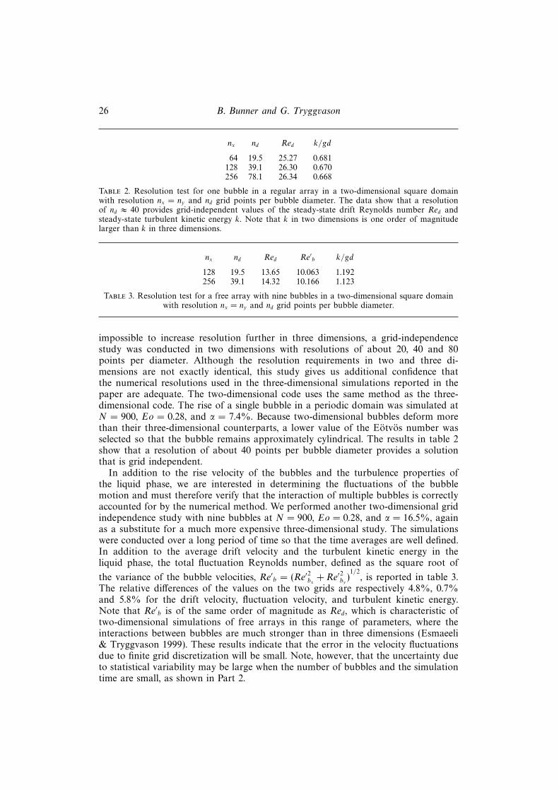
Table 1. Resolution tests for one bubble in a regular array in a cubic domain. As the number ofgrid points in the computational domain, nx = ny = nz , is increased, the number of grid pointsper bubble diameter, nd, increases in proportion. Tests were performed for three resolutions foreach value of α: coarse, intermediate and fine. The results show that the relative error between theintermediate and fine resolution is at most 4.4% for the steady-state drift Reynolds number of thebubble, Red, and 4.7% for the steady-state turbulent kinetic energy of the liquid phase, k.
Red
30
20
10
0 5 10 15 20 25
38.9 points per diameter20.4 points per diameter10.7 points per diameter
(a)
0 5 10 15 20 25
(b)0.05
0.04
0.03
0.02
0.01
kdg
t√(g/d ) t√(g/d )
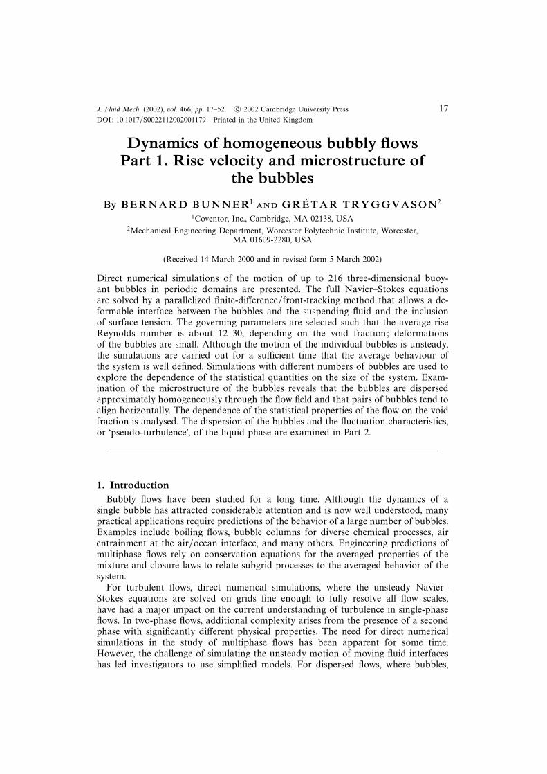
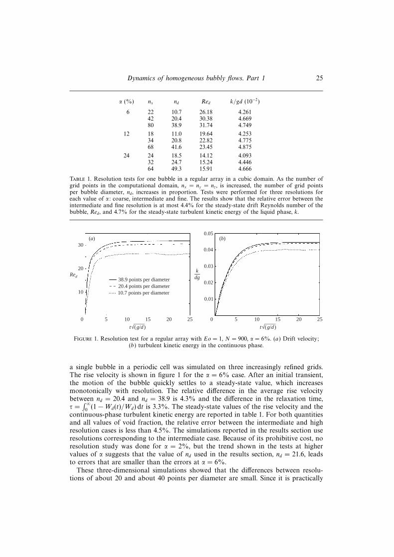
Figure 1. Resolution test for a regular array with Eo = 1, N = 900, α = 6%. (a) Drift velocity;(b) turbulent kinetic energy in the continuous phase.
a single bubble in a periodic cell was simulated on three increasingly refined grids.The rise velocity is shown in figure 1 for the α = 6% case. After an initial transient,the motion of the bubble quickly settles to a steady-state value, which increasesmonotonically with resolution. The relative difference in the average rise velocitybetween nd = 20.4 and nd = 38.9 is 4.3% and the difference in the relaxation time,τ =
∫ ∞0
(1−Wd(t)/Wd) dt is 3.3%. The steady-state values of the rise velocity and thecontinuous-phase turbulent kinetic energy are reported in table 1. For both quantitiesand all values of void fraction, the relative error between the intermediate and highresolution cases is less than 4.5%. The simulations reported in the results section useresolutions corresponding to the intermediate case. Because of its prohibitive cost, noresolution study was done for α = 2%, but the trend shown in the tests at highervalues of α suggests that the value of nd used in the results section, nd = 21.6, leadsto errors that are smaller than the errors at α = 6%.
These three-dimensional simulations showed that the differences between resolu-tions of about 20 and about 40 points per diameter are small. Since it is practically
26 B. Bunner and G. Tryggvason
nx nd Red k/gd
64 19.5 25.27 0.681128 39.1 26.30 0.670256 78.1 26.34 0.668
Table 2. Resolution test for one bubble in a regular array in a two-dimensional square domainwith resolution nx = ny and nd grid points per bubble diameter. The data show that a resolutionof nd ≈ 40 provides grid-independent values of the steady-state drift Reynolds number Red andsteady-state turbulent kinetic energy k. Note that k in two dimensions is one order of magnitudelarger than k in three dimensions.
nx nd Red Re′b k/gd
128 19.5 13.65 10.063 1.192256 39.1 14.32 10.166 1.123
Table 3. Resolution test for a free array with nine bubbles in a two-dimensional square domainwith resolution nx = ny and nd grid points per bubble diameter.
impossible to increase resolution further in three dimensions, a grid-independencestudy was conducted in two dimensions with resolutions of about 20, 40 and 80points per diameter. Although the resolution requirements in two and three di-mensions are not exactly identical, this study gives us additional confidence thatthe numerical resolutions used in the three-dimensional simulations reported in thepaper are adequate. The two-dimensional code uses the same method as the three-dimensional code. The rise of a single bubble in a periodic domain was simulated atN = 900, Eo = 0.28, and α = 7.4%. Because two-dimensional bubbles deform morethan their three-dimensional counterparts, a lower value of the Eotvos number wasselected so that the bubble remains approximately cylindrical. The results in table 2show that a resolution of about 40 points per bubble diameter provides a solutionthat is grid independent.
In addition to the rise velocity of the bubbles and the turbulence properties ofthe liquid phase, we are interested in determining the fluctuations of the bubblemotion and must therefore verify that the interaction of multiple bubbles is correctlyaccounted for by the numerical method. We performed another two-dimensional gridindependence study with nine bubbles at N = 900, Eo = 0.28, and α = 16.5%, againas a substitute for a much more expensive three-dimensional study. The simulationswere conducted over a long period of time so that the time averages are well defined.In addition to the average drift velocity and the turbulent kinetic energy in theliquid phase, the total fluctuation Reynolds number, defined as the square root of
the variance of the bubble velocities, Re′b = (Re′2bx + Re′2by )1/2
, is reported in table 3.The relative differences of the values on the two grids are respectively 4.8%, 0.7%and 5.8% for the drift velocity, fluctuation velocity, and turbulent kinetic energy.Note that Re′b is of the same order of magnitude as Red, which is characteristic oftwo-dimensional simulations of free arrays in this range of parameters, where theinteractions between bubbles are much stronger than in three dimensions (Esmaeeli& Tryggvason 1999). These results indicate that the error in the velocity fluctuationsdue to finite grid discretization will be small. Note, however, that the uncertainty dueto statistical variability may be large when the number of bubbles and the simulationtime are small, as shown in Part 2.
Dynamics of homogeneous bubbly flows. Part 1 27
2.5. Rise velocity of a single bubble
The rise velocity of a single bubble in an unbounded flow serves as a reference in thelimit when the void fraction tends to zero. Because the numerical code uses a uniformgrid and periodic boundary conditions, it is very expensive to calculate the motionof a bubble in an unbounded flow. Instead, an approximate value of the rise velocityis determined in this section from the numerical and experimental data availablein the literature. The drag coefficient is defined by CD = 8D/ 1
2ρfWT
2πd2, where
D = 16πd3(ρf−ρb)g is the drag and WT is the terminal velocity. CD is formally related
to the Eotvos, Morton and Galileo numbers by CD = 4Eo3/2/3Re2M1/2 = 4N/3Re2.Although a considerable amount of literature exists on the rise velocity of a bubble(Clift et al. 1978; Bhaga & Weber 1981; Ryskin & Leal 1984; Fan & Tschuyia 1990;Duineveld 1995; Maxworthy et al. 1996; McLaughlin 1996), very little of it is relevantto the situation of a contamination-free bubble that is slightly deformed with Eo = 1and N = 900. Most experiments have been performed in water and are stronglyaffected by surface-active agents, especially for small spherical bubbles.
Ryskin & Leal (1984) simulated the rise of a single bubble using a boundary-fittedfinite difference mesh. The data of figure 1 of their paper is interpolated to determineRe. For We ≈ 1, they report CD ≈ 1.43 for Re = 20 and CD ≈ 0.71 for Re = 50.By using a function of the form CD = (A/Re)(1 + (B/Re1/2)) and estimating theerror arising when reading the data from the figure, the rise Reynolds number isRe = 36.0± 1.5. A second, less accurate method to evaluate Re is to use a correlationfor contaminated drops and bubbles (Clift et al. 1978, pp. 176–178) to find Re ≈ 25.5,and to multiply this value by a correcting factor for a pure system. For Eo = 1, thisfactor is approximately 1.35, so that Re ≈ 34.5.
More data are available for bubbles that are exactly spherical, but they also exhibita considerable degree of scatter. Interpolating Ryskin & Leal’s data at We = 0 givesRe = 40.0 ± 1.5. A fit of numerical predictions of drag on spherical bubbles (Cliftet al. 1978, p. 130), CD = 14.9Re−0.78, gives Re = 36.5. Yuan & Prosperetti (1994)simulated the rise of two bubbles in line by a method similar to Ryskin & Leal’s.When the distance between the two bubbles is very large, the drag coefficient of theleading bubble can be used to estimate the drag coefficient of a single bubble in anunbounded flow, which results in Re = 38± 1.5.
A Galileo number N = 900 corresponds to an air bubble with a 0.452 mm diameterin water. Katz & Meneveau (1996) measured the terminal velocity of air bubbles inpurified water. For 0.475 mm diameter bubbles, they obtained Re = 35. Duineveld(1995) performed experiments in hyperdistilled water, but did not report results forbubbles that are as small. For contamined bubbles, Clift et al. (1978, p. 172) giveRe ≈ 20.7 and Nguyen (1998) gives Re ≈ 21.8 (the properties of water are takenat room temperature). As can be expected, this value agrees well with that obtainedfor a rigid sphere using a correlation for the standard drag curve (Clift et al. 1978,p. 112), which is Re = 21.4.
Since comparisons will be made with results from studies in the Stokes flow andpotential flow limits, the values obtained by using the drag laws in these limits arealso given here for completeness in the case of a spherical bubble at N = 900. InStokes flow, CD = 16/Re, which leads to Re = 75.0 for N = 900. In potential flow,CD = 48/Re, so that Re = 25.0.
To summarize, the rise Reynolds number that is taken as a reference for the caseof a single bubble rising steadily in an unbounded flow with Eo = 1 and N = 900 isthat derived from Ryskin & Leal’s paper, Re = 36.0, corresponding to CD = 0.93. For
28 B. Bunner and G. Tryggvason
a spherical bubble (Eo = 0) with N = 900, we take the average value of the threeresults cited above, Re = 38.0. Even if the scatter of the different sources is accountedfor, it seems that the finite Eotvos number has a small but noticeable effect on therise velocity. Therefore, we expect the quantitative results presented in this paper todiffer slightly from these that would be found for bubbles that are exactly spherical.This is discussed further below.
2.6. Effect of the surface tension
A 0.452 mm diameter air bubble in water has an Eotvos number of 0.0275 and isspherical. Small values of Eo lead to large numerical errors in the discretization of thesurface tension, characterized by the appearance of spurious currents. This problemis not unique to the front-tracking method, it appears also in the volume-of-fluid andlevel-set methods (Lafaurie et al. 1994). A simulation with Eotvos number Eo = 0.1and N = 900 was performed for a regular array with α = 6% on a 643 grid. Theresults were compared with the corresponding results for Eo = 1 in order to assessthe effect of surface tension and finite deformation. At steady state, the ratios of thelengths of the major axis and minor axis of the bubble is 1.08 for Eo = 1 and 1.006for Eo = 0.1. The relative differences of the steady-state values of the rise velocityand the turbulent kinetic energy of the liquid phase are 0.7% and 1.0% respectively.These differences are sufficiently small that the results of this paper are expected tobe relevant to spherical bubbles. The case of more deformable bubbles is discussed inBunner & Tryggvason (2002b), where fundamental differences are observed betweenEo = 1 and Eo = 5.
2.7. Effect of the density and viscosity ratios
The ratios of the densities and viscosities of the bubbles and the suspending fluid aretypically very small in most bubbly flows of interest. For example, for air bubbles inwater at room temperature, ρb/ρf = 1.22× 10⁻³ and µb/µf = 1.81× 10⁻². However,the multigrid solver used here fails to converge in the solution of equation (2.6) forthe pressure if the density ratio is very small. An SOR solver is more robust, butits use is impractical because it increases the computational time required to achievethe same accuracy by one to two orders of magnitude. Similar problems of increasedcomputational cost are encountered in boundary integral methods when the viscosityratio is different from one (Pozrikidis 1993; Loewenberg & Hinch 1996). We electedto increase ρb and µb, so that ρb/ρf = µb/µf = 1/50 in all simulations presented inthe results section. If the values of the density and the viscosity of the bubbles arevery small compared to the values of the surrounding fluid, the pressure and viscousforces exerted by the gaseous medium inside the bubble on the interface are small.Indeed, analytical solutions in the Stokes flow limit (Clift et al. 1978, p. 33) show thatif the viscosity of the bubble is one fiftieth the viscosity of the outer fluid, the risevelocity is reduced by only 1.0% compared to the rise velocity of a bubble with zeroviscosity. Likewise, the added mass coefficient of a bubble whose density is one fiftieththe density of the outer fluid is smaller than the added mass coefficient of a bubblewith zero density by 5.8% (Clift et al. 1978, p. 304). Numerical tests with our methodby Jan (1994) showed that ratios of 1/40 and 1/400 resulted in rise velocities thatdiffered by about 1.0%. The results of simulations with ρb/ρf = µb/µf = 1/50 shouldtherefore apply to situations where the density and viscosity ratios are much lower.Oka & Ishii (1999) arrived at the same conclusion in their numerical simulations ofgas bubbles using the level-set method.
Dynamics of homogeneous bubbly flows. Part 1 29
α(%) Nb L/d nx nd Tf√g/d Ti
√g/d zb/d zb/L nstep CPU procs
2 27 8.91 192 21.6 245 60 217 24.4 60720 80 83 13 6.10 128 21.0 126 35 109 17.8 25590 34 86 2 2.59 52 20.0 68 35 63 24.4 14510 — 16 4 3.27 64 19.6 57 35 48 14.6 11710 — 16 12 4.71 92 19.5 104 30 80 17.1 21250 50 46 27 6.18 128 20.7 257 30 183 28.7 58990 79 86 91 9.26 192 20.7 142 30 109 11.7 32430 54 86 216 12.35 256 20.7 142 30 109 8.8 32880 126 8
12 27 4.90 104 21.2 200 30 119 24.2 47710 78 812 54 6.18 128 20.7 111 40 74 12.0 29050 46 824 27 3.89 96 24.7 228 100 104 26.7 75030 88 8
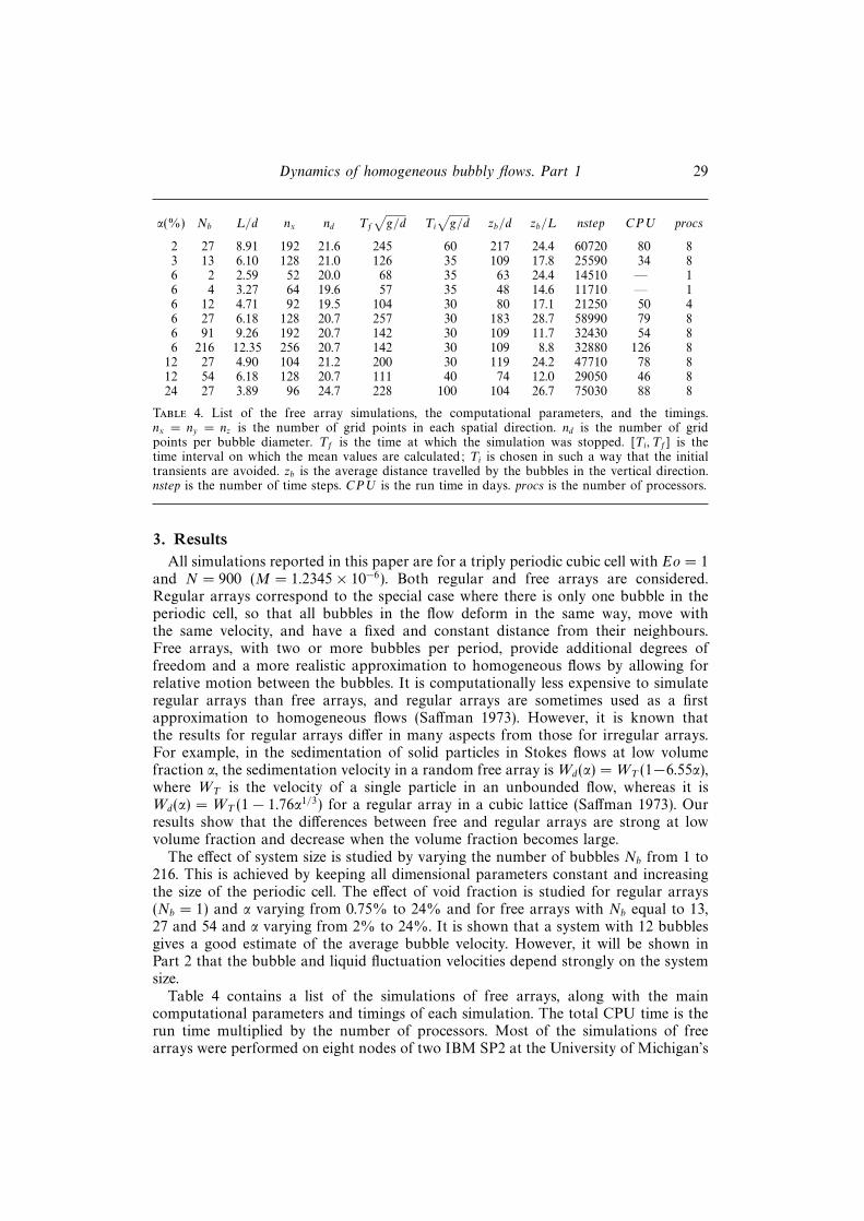
Table 4. List of the free array simulations, the computational parameters, and the timings.nx = ny = nz is the number of grid points in each spatial direction. nd is the number of gridpoints per bubble diameter. Tf is the time at which the simulation was stopped. [Ti, Tf] is thetime interval on which the mean values are calculated; Ti is chosen in such a way that the initialtransients are avoided. zb is the average distance travelled by the bubbles in the vertical direction.nstep is the number of time steps. CPU is the run time in days. procs is the number of processors.
3. ResultsAll simulations reported in this paper are for a triply periodic cubic cell with Eo = 1
and N = 900 (M = 1.2345× 10⁻⁶). Both regular and free arrays are considered.Regular arrays correspond to the special case where there is only one bubble in theperiodic cell, so that all bubbles in the flow deform in the same way, move withthe same velocity, and have a fixed and constant distance from their neighbours.Free arrays, with two or more bubbles per period, provide additional degrees offreedom and a more realistic approximation to homogeneous flows by allowing forrelative motion between the bubbles. It is computationally less expensive to simulateregular arrays than free arrays, and regular arrays are sometimes used as a firstapproximation to homogeneous flows (Saffman 1973). However, it is known thatthe results for regular arrays differ in many aspects from those for irregular arrays.For example, in the sedimentation of solid particles in Stokes flows at low volumefraction α, the sedimentation velocity in a random free array is Wd(α) = WT (1−6.55α),where WT is the velocity of a single particle in an unbounded flow, whereas it isWd(α) = WT (1 − 1.76α1/3) for a regular array in a cubic lattice (Saffman 1973). Ourresults show that the differences between free and regular arrays are strong at lowvolume fraction and decrease when the volume fraction becomes large.
The effect of system size is studied by varying the number of bubbles Nb from 1 to216. This is achieved by keeping all dimensional parameters constant and increasingthe size of the periodic cell. The effect of void fraction is studied for regular arrays(Nb = 1) and α varying from 0.75% to 24% and for free arrays with Nb equal to 13,27 and 54 and α varying from 2% to 24%. It is shown that a system with 12 bubblesgives a good estimate of the average bubble velocity. However, it will be shown inPart 2 that the bubble and liquid fluctuation velocities depend strongly on the systemsize.
Table 4 contains a list of the simulations of free arrays, along with the maincomputational parameters and timings of each simulation. The total CPU time is therun time multiplied by the number of processors. Most of the simulations of freearrays were performed on eight nodes of two IBM SP2 at the University of Michigan’s
30 B. Bunner and G. Tryggvason
Z
YX
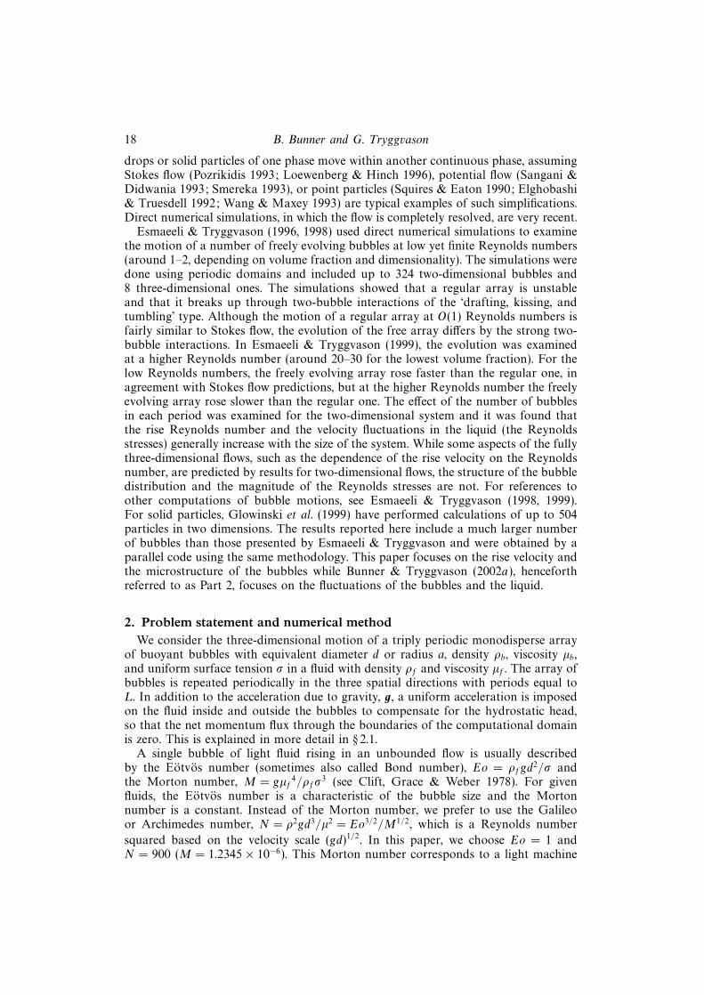
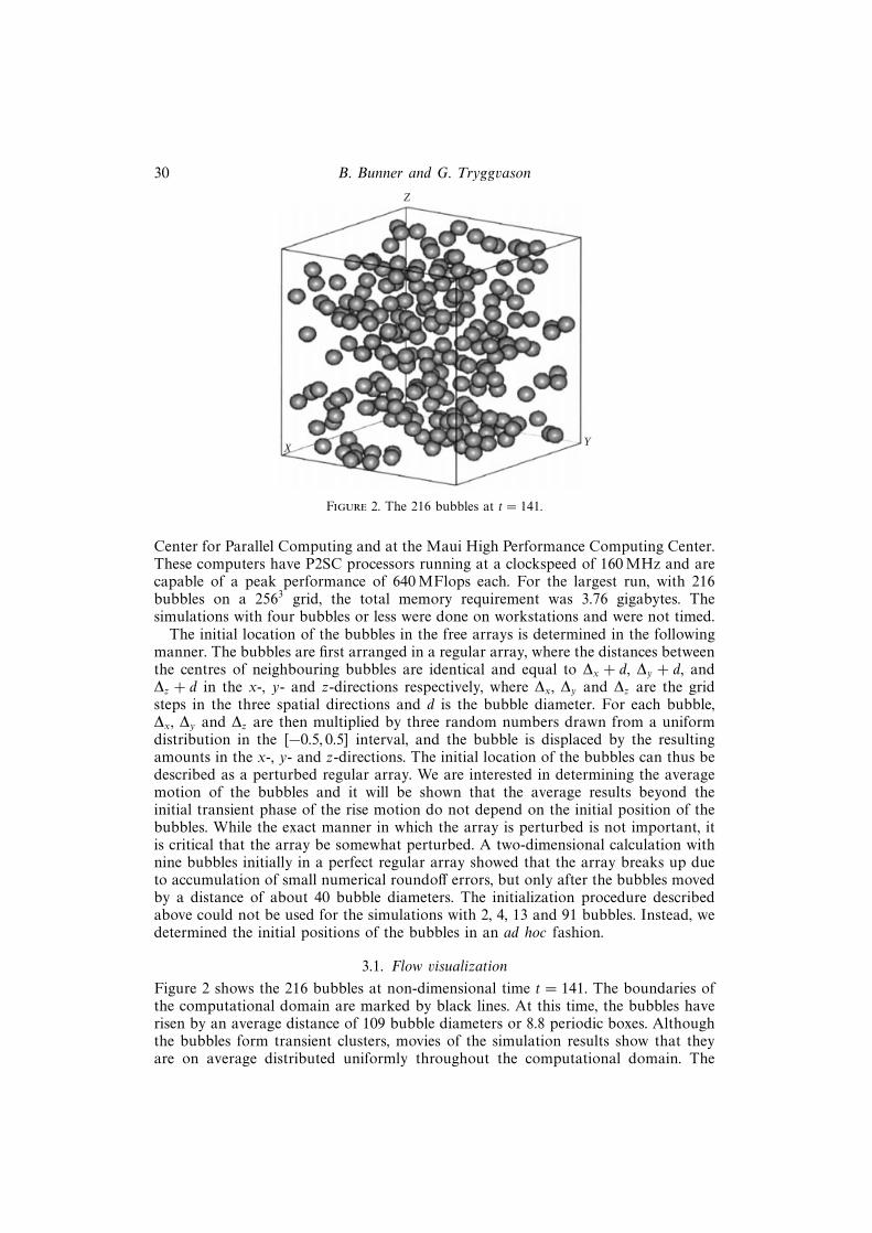
Figure 2. The 216 bubbles at t = 141.
Center for Parallel Computing and at the Maui High Performance Computing Center.These computers have P2SC processors running at a clockspeed of 160 MHz and arecapable of a peak performance of 640 MFlops each. For the largest run, with 216bubbles on a 2563 grid, the total memory requirement was 3.76 gigabytes. Thesimulations with four bubbles or less were done on workstations and were not timed.
The initial location of the bubbles in the free arrays is determined in the followingmanner. The bubbles are first arranged in a regular array, where the distances betweenthe centres of neighbouring bubbles are identical and equal to ∆x + d, ∆y + d, and∆z + d in the x-, y- and z-directions respectively, where ∆x, ∆y and ∆z are the gridsteps in the three spatial directions and d is the bubble diameter. For each bubble,∆x, ∆y and ∆z are then multiplied by three random numbers drawn from a uniformdistribution in the [−0.5, 0.5] interval, and the bubble is displaced by the resultingamounts in the x-, y- and z-directions. The initial location of the bubbles can thus bedescribed as a perturbed regular array. We are interested in determining the averagemotion of the bubbles and it will be shown that the average results beyond theinitial transient phase of the rise motion do not depend on the initial position of thebubbles. While the exact manner in which the array is perturbed is not important, itis critical that the array be somewhat perturbed. A two-dimensional calculation withnine bubbles initially in a perfect regular array showed that the array breaks up dueto accumulation of small numerical roundoff errors, but only after the bubbles movedby a distance of about 40 bubble diameters. The initialization procedure describedabove could not be used for the simulations with 2, 4, 13 and 91 bubbles. Instead, wedetermined the initial positions of the bubbles in an ad hoc fashion.
3.1. Flow visualization
Figure 2 shows the 216 bubbles at non-dimensional time t = 141. The boundaries ofthe computational domain are marked by black lines. At this time, the bubbles haverisen by an average distance of 109 bubble diameters or 8.8 periodic boxes. Althoughthe bubbles form transient clusters, movies of the simulation results show that theyare on average distributed uniformly throughout the computational domain. The
Dynamics of homogeneous bubbly flows. Part 1 31
Z
YX
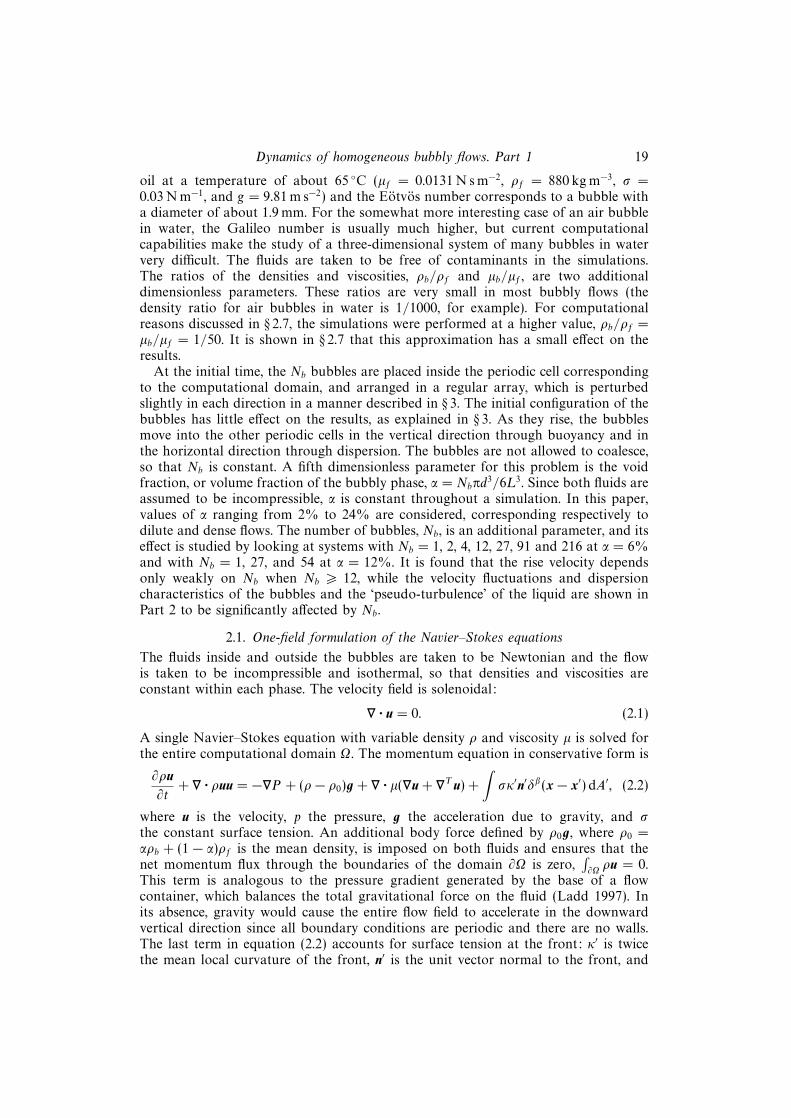
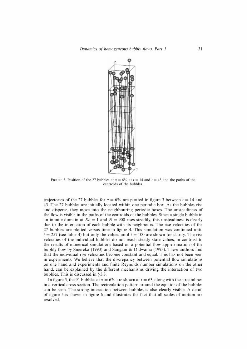
Figure 3. Position of the 27 bubbles at α = 6% at t = 14 and t = 43 and the paths of thecentroids of the bubbles.
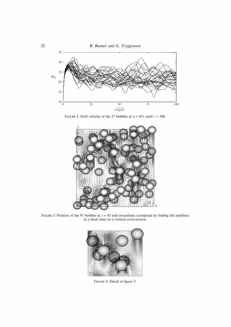
trajectories of the 27 bubbles for α = 6% are plotted in figure 3 between t = 14 and43. The 27 bubbles are initially located within one periodic box. As the bubbles riseand disperse, they move into the neighbouring periodic boxes. The unsteadiness ofthe flow is visible in the paths of the centroids of the bubbles. Since a single bubble inan infinite domain at Eo = 1 and N = 900 rises steadily, this unsteadiness is clearlydue to the interaction of each bubble with its neighbours. The rise velocities of the27 bubbles are plotted versus time in figure 4. This simulation was continued untilt = 257 (see table 4) but only the values until t = 100 are shown for clarity. The risevelocities of the individual bubbles do not reach steady state values, in contrast tothe results of numerical simulations based on a potential flow approximation of thebubbly flow by Smereka (1993) and Sangani & Didwania (1993). These authors findthat the individual rise velocities become constant and equal. This has not been seenin experiments. We believe that the discrepancy between potential flow simulationson one hand and experiments and finite Reynolds number simulations on the otherhand, can be explained by the different mechanisms driving the interaction of twobubbles. This is discussed in § 3.3.
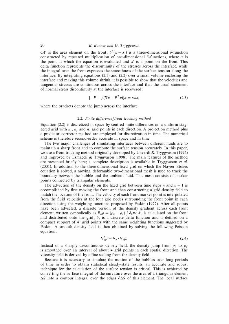
In figure 5, the 91 bubbles at α = 6% are shown at t = 63, along with the streamlinesin a vertical cross-section. The recirculation pattern around the equator of the bubblescan be seen. The strong interaction between bubbles is also clearly visible. A detailof figure 5 is shown in figure 6 and illustrates the fact that all scales of motion areresolved.
32 B. Bunner and G. Tryggvason
Red
35
30
100 25 50
t√(g/d )
20
25
15
75 100
Figure 4. Drift velocity of the 27 bubbles at α = 6% until t = 100.
Z
YX
Figure 5. Position of the 91 bubbles at t = 63 and streamlines (computed by finding the pathlinesat a fixed time) in a vertical cross-section.
Figure 6. Detail of figure 5.
Dynamics of homogeneous bubbly flows. Part 1 33
Red
30
0 50 100
t√(g/d )
20
25
150
(a)
(b)
Nb = 2169127121
Red
30
0 50 100
t√(g/d )
10
25
150
α = 2%
200 250
6%12%24%
35
20
15
5
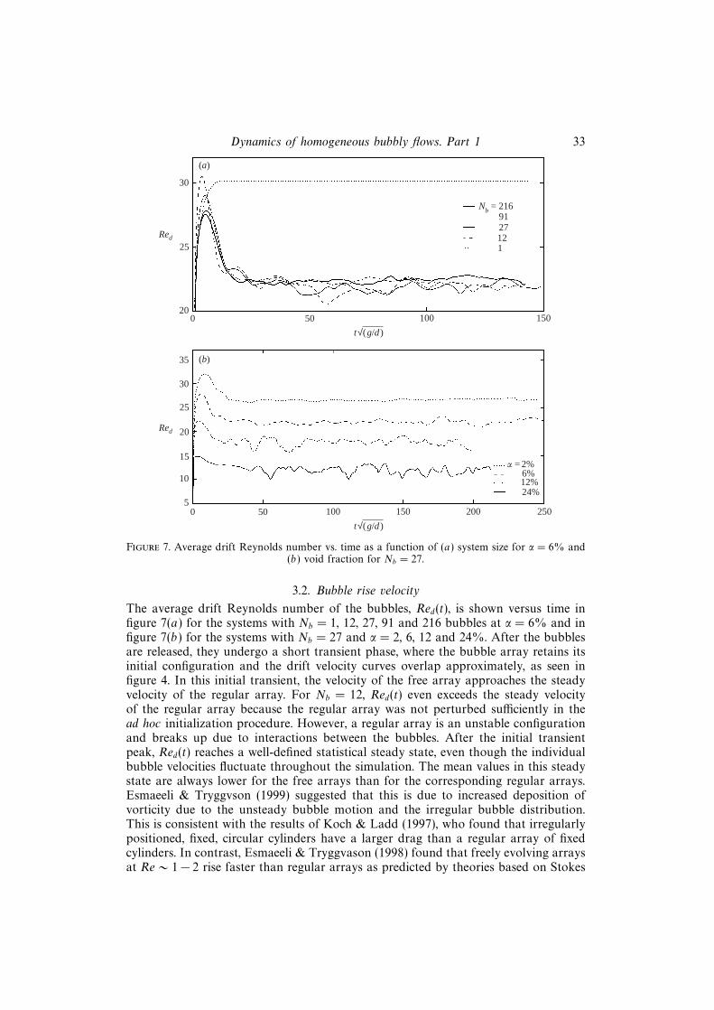
Figure 7. Average drift Reynolds number vs. time as a function of (a) system size for α = 6% and(b) void fraction for Nb = 27.
3.2. Bubble rise velocity
The average drift Reynolds number of the bubbles, Red(t), is shown versus time infigure 7(a) for the systems with Nb = 1, 12, 27, 91 and 216 bubbles at α = 6% and infigure 7(b) for the systems with Nb = 27 and α = 2, 6, 12 and 24%. After the bubblesare released, they undergo a short transient phase, where the bubble array retains itsinitial configuration and the drift velocity curves overlap approximately, as seen infigure 4. In this initial transient, the velocity of the free array approaches the steadyvelocity of the regular array. For Nb = 12, Red(t) even exceeds the steady velocityof the regular array because the regular array was not perturbed sufficiently in thead hoc initialization procedure. However, a regular array is an unstable configurationand breaks up due to interactions between the bubbles. After the initial transientpeak, Red(t) reaches a well-defined statistical steady state, even though the individualbubble velocities fluctuate throughout the simulation. The mean values in this steadystate are always lower for the free arrays than for the corresponding regular arrays.Esmaeeli & Tryggvson (1999) suggested that this is due to increased deposition ofvorticity due to the unsteady bubble motion and the irregular bubble distribution.This is consistent with the results of Koch & Ladd (1997), who found that irregularlypositioned, fixed, circular cylinders have a larger drag than a regular array of fixedcylinders. In contrast, Esmaeeli & Tryggvason (1998) found that freely evolving arraysat Re ∼ 1− 2 rise faster than regular arrays as predicted by theories based on Stokes
34 B. Bunner and G. Tryggvason
Red
30
1 2
20
25
(a)
(b)
α = 6%
Red
40
0 2
20
35
35
154 12 27 54 91 216
Nb
12%
α (%)
Free arrayRegular arrayReTReb = 36.0 (1–α1/3)Reb = 29.0 (1–4.0α)
30
25
15
103 6 12 24
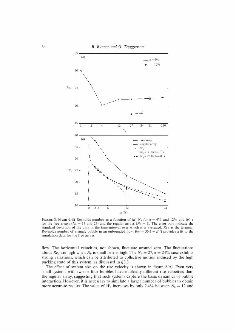
Figure 8. Mean drift Reynolds number as a function of (a) Nb for α = 6% and 12% and (b) αfor the free arrays (Nb = 13 and 27) and the regular arrays (Nb = 1). The error bars indicate thestandard deviation of the data in the time interval over which it is averaged. ReT is the terminalReynolds number of a single bubble in an unbounded flow. Reb = 36(1− α0.3) provides a fit to thesimulation data for the free arrays.
flow. The horizontal velocities, not shown, fluctuate around zero. The fluctuationsabout Red are high when Nb is small or α is high. The Nb = 27, α = 24% case exhibitsstrong variations, which can be attributed to collective motion induced by the highpacking state of this system, as discussed in § 3.3.
The effect of system size on the rise velocity is shown in figure 8(a). Even verysmall systems with two or four bubbles have markedly different rise velocities thanthe regular array, suggesting that such systems capture the basic dynamics of bubbleinteraction. However, it is necessary to simulate a larger number of bubbles to obtainmore accurate results. The value of Wd increases by only 2.4% between Nb = 12 and
Dynamics of homogeneous bubbly flows. Part 1 35
Nb = 216 so that the average drift velocity can be considered effectively independentof Nb when Nb > 12. Since the initial configurations of the bubble arrays are differentin the simulations with Nb = 12, 27, 91 and 216 bubbles, this also indicates that theinitial positions of the bubbles have no influence on the average drift velocity pastthe initial transient peak.
System size effects are important in simulations of sedimenting particles at lowReynolds number due to the long range of particle–particle interactions. For example,in the Stokes flow simulations of Ladd (1993), a difference of 5–10% can be seen inthe sedimentation velocity when 32 and 108 particles are used at a volume fraction of5%. At high Reynolds numbers, the velocity disturbance induced by a bubble decaysmuch faster with distance away from the bubble than in Stokes flow. Sangani, Zhang& Prosperetti (1991) report that the average bubble velocity in their potential flowsimulations changes very little for 8, 16, and 32 bubbles.
The ability to predict the dependence of the average velocity on the volumefraction is of fundamental importance in the study of dispersed multiphase flows.A brief summary of existing results for bubbles follows. van Wijngaarden (1993)determined the rise velocity of equisized spherical bubbles in dilute conditions in thecase where the Reynolds number is sufficiently high that the flow can be assumedto be potential, yet the Weber number is sufficiently small that the bubbles remainspherical. From an analysis of the relative motion of a pair of bubbles, he found thatthe most likely orientation of the separation vector between the two bubbles is in aplane perpendicular to gravity and derived the pair probability distribution functionin this plane. Using this probability density, he calculated the average rise velocity tothe leading order:
Wd(α) = WT (1− 1.56α). (3.1)
For comparison, he also determined the mean rise velocity by assuming that thebubbles are randomly distributed in space and randomly distributed in a horizontalplane and found, respectively,
Wd(α) = WT (1− 2α) (3.2)
and
Wd(α) = WT (1− 1.25α). (3.3)
The effect of the microstructure on the average rise velocity is clear. Experimentalconfirmation of the linear dependence of Wd on α in the high Reynolds numberregime, Re > 200, was made for air bubbles in purified water by van Wijngaarden &Kapteyn (1990), who found
Wd(α) = V (1− 1.78α), (3.4)
but only for 0.02 < α < 0.15. Between α = 0 and 2%, Wd(α) falls nonlinearly, V being20% lower than the terminal rise velocity WT . A similar sharp drop between Wd(0)and Wd(α > 0) was observed by Zenit, Koch & Sangani (2001) in their experimentson slightly deformed bubbles at Reynolds number about 300. For α > 0, they found:
Wd(α) ∝ (1− α)2.8. (3.5)
For the general case of particulate flows at a wide range of Reynolds numbers anddeformations, Ishii & Zuber (1979) assumed a similarity criterion between the draglaw of a single particle and the drag law of a multi-particle system and used a vastnumber of experimental data to determine Wd(α). For bubbles, they distinguish fourregimes as the Reynolds number increases: Stokes regime, viscous regime, distorted
36 B. Bunner and G. Tryggvason
particle regime, and churn turbulent regime. The high Reynolds number experimentalresults of van Wijngaarden & Kapteyn (1990) fall into the distorted particle regime,for which Ishii & Zuber (1979) propose
Wd(α) = WT (1− α)1.75, (3.6)
which agrees well with equation (3.4) when α is small, and also with the formulagiven in Hetsroni (1982, pp. 2–87). Our results are for lower Reynolds number andfall into the viscous regime, where a more complicated formula applies. However, inthe range of void fraction considered here, the Ishii & Zuber (1979) correlation canbe approximated by
Wd(α) ≈WT (1− α)3.0. (3.7)
These correlations, equations (3.6) and (3.7), are derived by scaling and validatedwith experimental data where surface contamination plays an important role. Theirdirect applicability to the current results is therefore questionable, but they will serveas useful reference points. In particular, linear and power-law fits will be attemptedand comparisons made with the formulae presented above.
The mean drift velocity computed from our results is shown versus α in figure 8(b);α ranges from 0.75% to 24% for the regular arrays and from 2% to 24% for the freearrays. The regular array results are discussed at the end of the section. Due to thehigh cost of simulating a system with a large number of bubbles at very small voidfractions with our code, the lowest void fraction reported here for a free array is 2%,for which Red = 26.6. Nevertheless, as α approaches zero, Red(α) must tend towardsthe terminal velocity of a single bubble in an unbounded flow determined in § 2.5,ReT = 36.0, implying a sharp decrease in the rise velocity from α = 0 to α = 2%.Unlike the analytical results of van Wijngaarden (1993) and the experimental resultsof van Wijngaarden & Kapteyn (1990), which are both for much higher Reynoldsnumbers, Red(α) is not a linear function of α, but is slightly convex. However, if wefit lines between α = 2% and 6% on one hand and between α = 2% and 24% on theother hand, the slopes are in both cases higher than the slopes of equations (3.1) to(3.4), but consistent with a linearization of equation (3.7) at small α. The projectionsof these fits on α = 0 give Red = 28.4 ± 0.7 in both cases, which is about 25%lower than ReT . The fact that Red < ReT and the magnitude of the difference arein agreement with the experimental results of van Wijngaarden & Kapteyn (1990)and Zenit et al. (2001). Zenit et al. (2001) attribute the sharp decrease of the meanbubble velocity at low void fractions to the collisions of the bubbles with the walls oftheir experimental channel. The absence of walls in our simulations shows that thisfactor is probably not the main reason. We believe that this nonlinear decrease is dueto the change in microstructure. For α = 0, the bubbles are distributed randomly inspace and do not interact with their neighbours. For α = 2%, bubbles tend to alignthemselves horizontally relative to their neighbors, as shown in § 3.3. This change inthe microstructure results in a higher drag coefficient and therefore lower rise velocitythan for bubbles at α = 0. A power law of the form of equations (3.6) and (3.7) doesnot provide a good fit to the computed values of Wd(α) and WT , but a good fit isgiven by:
Red = 36.0(1− α0.3). (3.8)
This expression is robust to small variations in ReT in the simulations results, withonly small changes in the exponent. It is emphasized that there is no theoreticaljustification for this formula.
The velocity of the regular array is greater than that of the free array for all values

Dynamics of homogeneous bubbly flows. Part 1 37
of void fraction reported here. This can also be attributed to the difference in themicrostructure. The regular array contains an equal number of bubble pairs alignedhorizontally and vertically, whereas the free array contains a larger number of bubblepairs that are aligned horizontally. Since the drag of a horizontally aligned bubblepair is larger than the drag of a vertically aligned bubble pair, where the wake ofthe leading bubble shields the trailing bubble from the oncoming flow, the bubblesrise faster in the regular array than in the free array. At low void fractions, the driftReynolds number in the regular arrays is higher than ReT . Therefore Red(α) actuallyincreases with α for values of α between 0 and 0.75%. The following explanation issuggested for this behavior. As mentioned previously, a bubble trailing in the wakeof another bubble experiences a lower drag than an isolated bubble. In a regulararray, every bubble is located in the wake of an infinite number of bubbles (itsperiodic images). At low void fractions, this tends to reduce the drag of the bubbleand increase its rise velocity to a value larger than WT . At high void fraction, theflow blockage due to the presence of the surrounding bubbles starts dominating overthis drag reduction mechanism, so that Red eventually becomes smaller than ReT .
3.3. Microstructure
The discussion and results above have made clear the importance of understanding thespatial distribution of the bubbles and the fundamental mechanisms which determinethe interactions between them. Approximate knowledge of the microstructure oran assumption about the microstructure is necessary to determine the rise velocityanalytically (van Wijngaarden 1993). Moreover, Smereka (1993) pointed out that awrong assumption about the microstructure can lead to ill-posed models. A summaryof previous studies regarding the bubble distribution is given here, starting with theinteraction of two side-by-side bubbles and two in-line bubbles, moving on to multi-bubble systems in the potential flow approximation, and finishing with work at finiteReynolds numbers.
Two spheres in steady potential flow attract when they move perpendicularly totheir line of centres and repel when they move in the direction parallel to their line ofcentres (Lamb 1932). Legendre & Magnaudet (1998) considered the motion of twospherical bubbles whose line of centres is perpendicular to the direction of motionand which are separated by a fixed distance r = sa, where a is the radius of thebubbles. In the potential flow limit, they report that the rise velocity is lower thanthe terminal velocity of an isolated bubble and that the bubbles are always attractedtowards each other. The reason for this attractive force is that the pressure in thegap between the bubbles is lower than the ambient pressure. In the opposite limit ofvery viscous flows where the Oseen approximation is valid and small inertia effectsare present, they report that the bubbles always repel and that the rise velocity islower than the terminal velocity at short separation distances and higher at largeseparation distances. In the absence of inertia, the lift force is zero and the bubblesdo not experience relative motion unless acted upon by a third bubble. Legendre &Magnaudet (1998) computed the motion of two side by side bubbles at 0.1 6 Re 6 500by solving the Navier–Stokes equations and confirmed the validity of the expressionsderived from the Oseen approximation at low Re. They found that the lift forcechanges sign at 2.5 6 Re 6 25 for separation distances 3 6 s 6 10. However, theywere unable to recover the predictions of potential flow theory, even at Re as large as500 and attributed the discrepancy to vorticity generated at the surface of the bubble.
Harper (1970) analysed the rise of two bubbles in line at a fixed separation distanceunder the assumption of potential flow but with the inclusion of a thin wake between
38 B. Bunner and G. Tryggvason
the bubbles. He determined that the irrotational interaction results in an O(s−4)repulsive force due to the pressure being higher in the gap between the bubblesthan in the ambient flow, while the wake effect tends to move the bubbles towardseach other, so that there exists an equilibrium distance at which the hydrodynamicforces balance. This equilibrium distance is stable to vertical displacements, but avertical line of two bubbles is unstable to lateral displacements. Yuan & Prosperetti(1994) computed the in-line motion of two spherical bubbles at Re up to 200 bysolving the unsteady Navier–Stokes equations. Their results agree qualitatively withHarper’s (1970) theory, in particular in the existence of an equilibrium distance, butthe values of the drag differ considerably, even for Re = 200. They also show thatthe transport and diffusion of vorticity affect the interaction between the bubblesvery strongly. Katz & Meneveau (1996) conducted experiments of nearly sphericalin-line air bubbles in purified water for 0.2 6 Re 6 140. Contrary to the results ofHarper’s (1970) first-order boundary layer theory and Yuan & Prosperetti’s (1994)Navier–Stokes simulations, they observe that the bubbles always collide and coalesce,indicating that the adverse pressure gradient is not strong enough to overcome thewake effect. Katz & Meneveau (1996) and Yuan & Prosperetti (1994) suggest thatthe discrepancy between the experimental and numerical results is due to bubbledeformation.
The unsteady motion of a pair of spherical bubbles was studied in the potentialflow approximation by Biesheuvel & van Wijngaarden (1982), Kok (1989), and vanWijngaarden (1993). When the angle θ between the line joining the bubble centresand the direction of gravity is smaller than 55 or larger than 125, the two bubblesrepel each other. When θ lies between these two values, they attract each other. Thesimulations and experiments of Kok (1989) show that two bubbles always approacheach other along a line inclined at an angle close to π/2 and that they move towardseach other until they touch. At close encounter, the bubbles bounce in singly filtratedwater but coalesce in hyperfiltrated water. The first result was used by van Wijngaar-den (1993), who assumed that the motion of a bubble pair is entirely in a horizontalplane in order to determine the probability density function of finding two bubblesat a given distance of each other and to calculate the average rise velocity of a dilutesuspension. van Wijngaarden (1993) also showed that the second result, i.e. that thebubbles touch, leads to clustering of pairs when viscosity is present. He noted that,while the formation of horizontal bubble clusters is observed in the transition frombubbly flow to slug flow, clustering is not observed in experiments at volume concen-trations well below this transition. He argued that clustering may be prevented by theeffect of multiple interactions and by turbulence. However, an attempt to calculatethe interaction of a third bubble with a bubble pair was inconclusive, suggestingthat multiple potential interactions are not able to compensate for the tendency tocluster.
The motion of a large number of spherical bubbles in potential flow was studiednumerically by Sangani & Didwania (1993), Smereka (1993), and Yurkovetsky &Brady (1996). Although the particular approaches differ, they share key features. Theviscous forces are included by using Levich’s expression for the drag, F = 12πµaV r ,or by differentiation of the rate of viscous energy dissipation, F = 1
2∇Ed. It is assumed
that colliding bubbles bounce without coalescing and that the momentum and kineticenergy of the system are conserved throughout the collision. The results of the threestudies are similar. In the absence of gravity and viscous forces, when the bubblesare given initial velocities with mean in the vertical direction, they form horizontalclusters if the variance of the velocity is small, but remain randomly distributed if
Dynamics of homogeneous bubbly flows. Part 1 39
the initial velocity distribution is sufficiently non-uniform. When gravity and viscousforces are included, the bubbles always aggregate in horizontal clusters. Smereka(1993) suggested that liquid turbulence may inhibit this clustering since it wouldincrease the variance of the bubble velocities. Sangani & Didwania (1993) recognizedthat the assumption of an irrotational flow might be an oversimplification and that itmight be necessary to include vorticity in the model, possibly as an additional randomforce on the bubbles. Zenit et al. (2001) found that some horizontal clustering occursin experiments with bubbles at Reynolds number about 300, but not to the extentpredicted by potential flow theory.
Fortes, Joseph & Lundgren (1987) examined the motion of solid spherical particlesfluidized in water at high Reynolds numbers. For two spheres initially aligned verti-cally, they observed that the trailing particle is drafted into the wake of the leadingparticle. After the two particles come into contact, they rotate around each otherand move away from each other while falling side by side. Fortes et al. (1987) calledthis fundamental rearrangement mechanism ‘drafting, kissing, and tumbling’. Theyalso looked at a cross-stream alignment of spheres fluidized by a water stream andnoticed that the cross-stream array was a stable configuration. In fluidized beds withmuch larger numbers of particles at volume concentrations between 10% and 28%,they observed that these cross-stream arrays are an important feature of the flow,along with the breaking down of falling streamwise particle pairs. Direct numericalsimulations of two sedimenting spheres by Feng, Hu & Joseph (1994) showed thatthe drafting, kissing, and tumbling mechanism accounts well for the interaction ofparticles at finite Reynolds numbers.
Cartellier & Riviere (2001) performed experiments with nearly spherical bubblesat α < 1%. They found that bubbles at Re = O(1) are approximately uniformly dis-tributed whereas bubbles at Re = O(10) exhibit a preference for horizontal alignment.Esmaeeli & Tryggvason (1998, 1999) likewise found that the tendency for bubblesto line up horizontally increases with Reynolds number. In addition, Cartellier &Riviere (2001) examined the interaction of two bubbles, which are initially alignedvertically, in the case where the bubbles are clean and in the case where the bubblesare contamined. They found that contaminated bubbles experience drafting, kissingand tumbling, but that clean bubbles rarely collide, instead smoothly rotating aroundeach other. Their results suggest that the discrepancy mentioned above between theresults of Katz & Meneveau (1996) and Yuan & Prosperetti (1994) might be due tosurface contamination rather than bubble deformation.
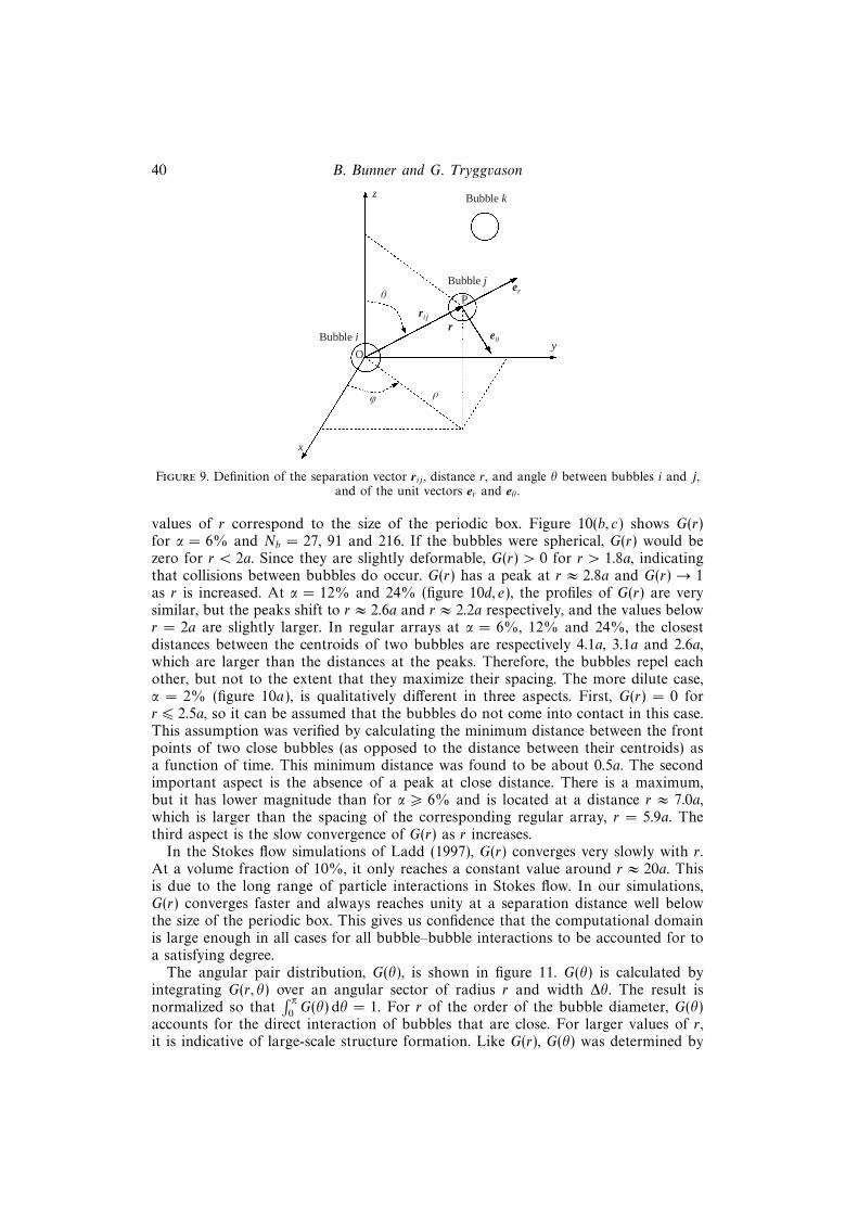
In order to understand the microstructure of bubble interactions, we examine thepair probability distribution function, G(r, θ), which is defined as the probability thatthe separation vector rij between the centroids of bubbles i and j has norm r and isoriented at an angle θ with respect to the direction of gravity:
G(r, θ) =Ω
Nb(Nb − 1)
⟨∑i=1,Nb
∑j=1,Nb
i6=j
δ(r − rij)⟩. (3.9)
Here Ω is the volume of the periodic cell. The configuration of bubbles i and jis illustrated in figure 9. The radial pair distribution function, G(r), defined as theintegral of G(r, θ) over thin spherical shells of width ∆r and radius r, is shown infigure 10. The results were obtained by averaging over at least 200 evenly spaced timesamples in the [Ti, Tf] time intervals. Nearly identical results were obtained when ∆rand the number of time samples were divided or multiplied by two. The maximum
40 B. Bunner and G. Tryggvason
ρ
θ
z
x
y
ri jr
Bubble k
Bubble j
Bubble i
er
eθ
P
O
Figure 9. Definition of the separation vector rij , distance r, and angle θ between bubbles i and j,and of the unit vectors er and eθ .
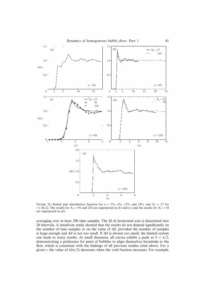
values of r correspond to the size of the periodic box. Figure 10(b, c) shows G(r)for α = 6% and Nb = 27, 91 and 216. If the bubbles were spherical, G(r) would bezero for r < 2a. Since they are slightly deformable, G(r) > 0 for r > 1.8a, indicatingthat collisions between bubbles do occur. G(r) has a peak at r ≈ 2.8a and G(r) → 1as r is increased. At α = 12% and 24% (figure 10d, e), the profiles of G(r) are verysimilar, but the peaks shift to r ≈ 2.6a and r ≈ 2.2a respectively, and the values belowr = 2a are slightly larger. In regular arrays at α = 6%, 12% and 24%, the closestdistances between the centroids of two bubbles are respectively 4.1a, 3.1a and 2.6a,which are larger than the distances at the peaks. Therefore, the bubbles repel eachother, but not to the extent that they maximize their spacing. The more dilute case,α = 2% (figure 10a), is qualitatively different in three aspects. First, G(r) = 0 forr 6 2.5a, so it can be assumed that the bubbles do not come into contact in this case.This assumption was verified by calculating the minimum distance between the frontpoints of two close bubbles (as opposed to the distance between their centroids) asa function of time. This minimum distance was found to be about 0.5a. The secondimportant aspect is the absence of a peak at close distance. There is a maximum,but it has lower magnitude than for α > 6% and is located at a distance r ≈ 7.0a,which is larger than the spacing of the corresponding regular array, r = 5.9a. Thethird aspect is the slow convergence of G(r) as r increases.
In the Stokes flow simulations of Ladd (1997), G(r) converges very slowly with r.At a volume fraction of 10%, it only reaches a constant value around r ≈ 20a. Thisis due to the long range of particle interactions in Stokes flow. In our simulations,G(r) converges faster and always reaches unity at a separation distance well belowthe size of the periodic box. This gives us confidence that the computational domainis large enough in all cases for all bubble–bubble interactions to be accounted for toa satisfying degree.
The angular pair distribution, G(θ), is shown in figure 11. G(θ) is calculated byintegrating G(r, θ) over an angular sector of radius r and width ∆θ. The result isnormalized so that
∫ π0G(θ) dθ = 1. For r of the order of the bubble diameter, G(θ)
accounts for the direct interaction of bubbles that are close. For larger values of r,it is indicative of large-scale structure formation. Like G(r), G(θ) was determined by
Dynamics of homogeneous bubbly flows. Part 1 41
1.0
20
0.5
(a) (b)
α = 2%
1.5
5 10 15
G(r)
α = 6%
1.0
20
0.5
1.5
5 10 15
Nb = 27216
1.0
10
0.5
(c) (d )
α = 6%
1.5
2 3 5
G(r)
α = 12%
1.0
20
0.5
1.5
6 8 10
Nb = 2754
1.0
20
0.5
(e)
α = 24%
1.5
4 6 8
G(r)
1244
2.0
r/a
r/a r/a
20 25
Nb = 2791216
Figure 10. Radial pair distribution function for α = 2%, 6%, 12% and 24% and Nb = 27 forr ∈ [0, L]. The results for Nb = 91 and 216 are superposed in (b) and (c) and the results for Nb = 54are superposed in (d ).
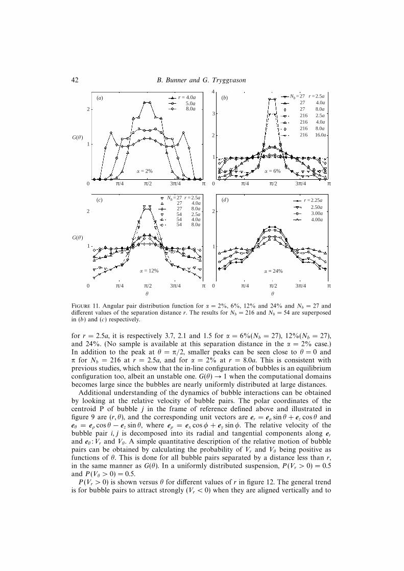
averaging over at least 200 time samples. The [0, π] horizontal axis is discretized into20 intervals. A sensitivity study showed that the results do not depend significantly onthe number of time samples or on the value of ∆θ, provided the number of samplesis large enough and ∆θ is not too small. If ∆θ is chosen too small, the limited systemsize leads to noisy results. At small distances, all curves exhibit a peak at θ = π/2,demonstrating a preference for pairs of bubbles to align themselves broadside to theflow, which is consistent with the findings of all previous studies cited above. For agiven r, the value of G(π/2) decreases when the void fraction increases. For example,
42 B. Bunner and G. Tryggvason
π /40
(a) (b)
α = 2%
2
G(õ )
3
2
4Nb = 27 r = 2.5a
1
(c) (d )
α = 12%
2
G(õ )
α = 24%
õ
π /2 3π /4 π
r = 4.0a5.0a8.0a
1
2727216216216216
4.0a8.0a2.5a4.0a8.0a16.0a
α = 6%
Nb = 27 r = 2.5a2727545454
4.0a8.0a2.5a4.0a8.0a
π /40 π /2 3π /4 π
π /40 π /2 3π /4 π π /40 π /2 3π /4 πõ
r = 2.25a
2.50a3.00a4.00a
1
2
1
Figure 11. Angular pair distribution function for α = 2%, 6%, 12% and 24% and Nb = 27 anddifferent values of the separation distance r. The results for Nb = 216 and Nb = 54 are superposedin (b) and (c) respectively.
for r = 2.5a, it is respectively 3.7, 2.1 and 1.5 for α = 6%(Nb = 27), 12%(Nb = 27),and 24%. (No sample is available at this separation distance in the α = 2% case.)In addition to the peak at θ = π/2, smaller peaks can be seen close to θ = 0 andπ for Nb = 216 at r = 2.5a, and for α = 2% at r = 8.0a. This is consistent withprevious studies, which show that the in-line configuration of bubbles is an equilibriumconfiguration too, albeit an unstable one. G(θ)→ 1 when the computational domainsbecomes large since the bubbles are nearly uniformly distributed at large distances.
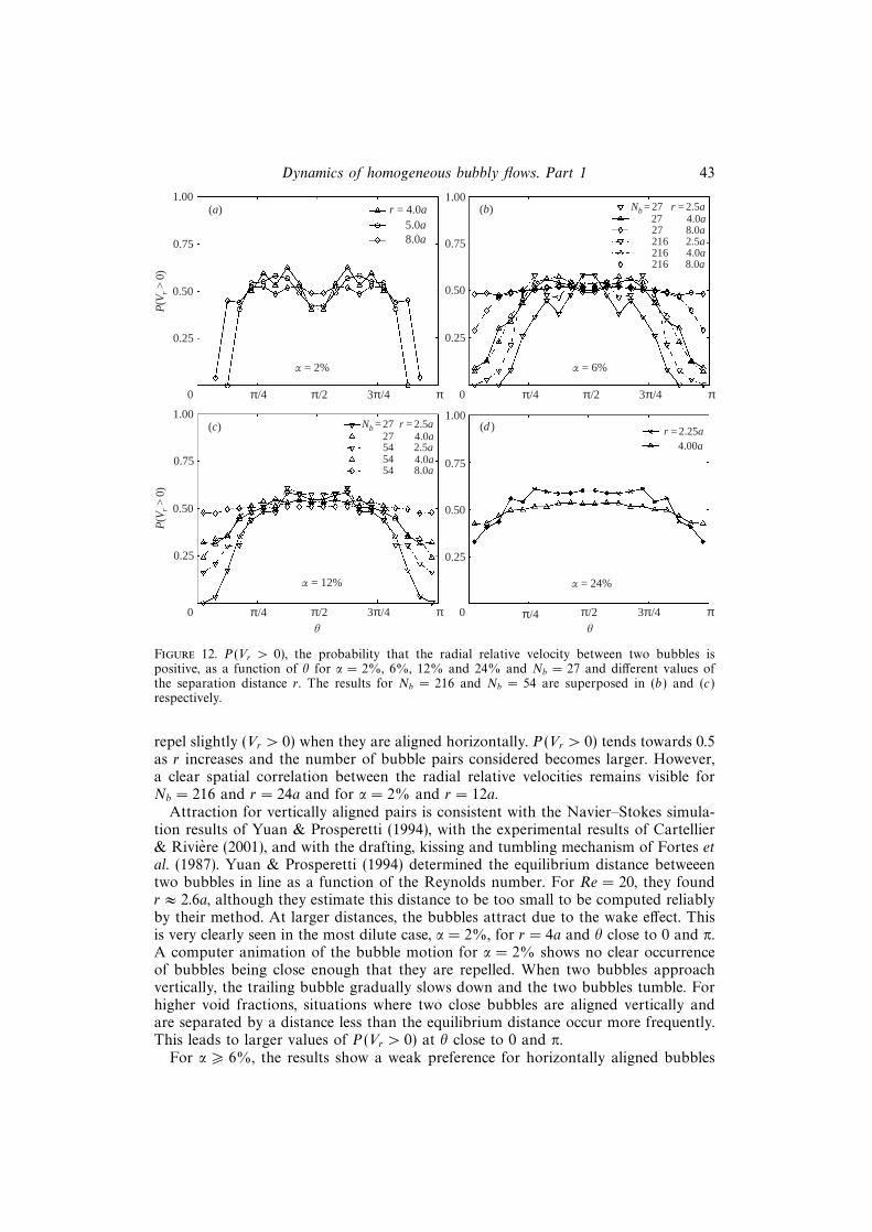
Additional understanding of the dynamics of bubble interactions can be obtainedby looking at the relative velocity of bubble pairs. The polar coordinates of thecentroid P of bubble j in the frame of reference defined above and illustrated infigure 9 are (r, θ), and the corresponding unit vectors are er = eρ sin θ + ez cos θ andeθ = eρ cos θ − ez sin θ, where eρ = ex cosφ + ey sinφ. The relative velocity of thebubble pair i, j is decomposed into its radial and tangential components along erand eθ:Vr and Vθ . A simple quantitative description of the relative motion of bubblepairs can be obtained by calculating the probability of Vr and Vθ being positive asfunctions of θ. This is done for all bubble pairs separated by a distance less than r,in the same manner as G(θ). In a uniformly distributed suspension, P (Vr > 0) = 0.5and P (Vθ > 0) = 0.5.P (Vr > 0) is shown versus θ for different values of r in figure 12. The general trend
is for bubble pairs to attract strongly (Vr < 0) when they are aligned vertically and to
Dynamics of homogeneous bubbly flows. Part 1 43
π /40
(a) (b)
α = 2%
1.00
P(V
r>
0)
0.75
0.50
1.00Nb = 27 r = 2.5a
(c) (d )
α = 12% α = 24%
õ
π /2 3π /4 π
r = 4.0a5.0a8.0a
0.25
2727216216216
4.0a8.0a2.5a4.0a8.0a
α = 6%
Nb = 27 r = 2.5a27545454
4.0a2.5a4.0a8.0a
π /40 π /2 3π /4 π
π /40 π /2 3π /4 π π /40 π /2 3π /4 πõ
r = 2.25a4.00a
0.75
0.50
0.25
0.75
0.50
1.00
0.25
1.00
P(V
r>
0)
0.75
0.50
0.25
Figure 12. P (Vr > 0), the probability that the radial relative velocity between two bubbles ispositive, as a function of θ for α = 2%, 6%, 12% and 24% and Nb = 27 and different values ofthe separation distance r. The results for Nb = 216 and Nb = 54 are superposed in (b) and (c)respectively.
repel slightly (Vr > 0) when they are aligned horizontally. P (Vr > 0) tends towards 0.5as r increases and the number of bubble pairs considered becomes larger. However,a clear spatial correlation between the radial relative velocities remains visible forNb = 216 and r = 24a and for α = 2% and r = 12a.
Attraction for vertically aligned pairs is consistent with the Navier–Stokes simula-tion results of Yuan & Prosperetti (1994), with the experimental results of Cartellier& Riviere (2001), and with the drafting, kissing and tumbling mechanism of Fortes etal. (1987). Yuan & Prosperetti (1994) determined the equilibrium distance betweeentwo bubbles in line as a function of the Reynolds number. For Re = 20, they foundr ≈ 2.6a, although they estimate this distance to be too small to be computed reliablyby their method. At larger distances, the bubbles attract due to the wake effect. Thisis very clearly seen in the most dilute case, α = 2%, for r = 4a and θ close to 0 and π.A computer animation of the bubble motion for α = 2% shows no clear occurrenceof bubbles being close enough that they are repelled. When two bubbles approachvertically, the trailing bubble gradually slows down and the two bubbles tumble. Forhigher void fractions, situations where two close bubbles are aligned vertically andare separated by a distance less than the equilibrium distance occur more frequently.This leads to larger values of P (Vr > 0) at θ close to 0 and π.
For α > 6%, the results show a weak preference for horizontally aligned bubbles
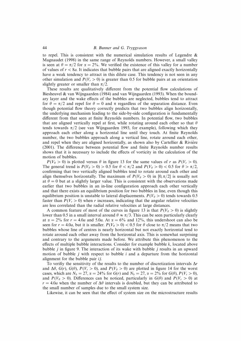
44 B. Bunner and G. Tryggvason
to repel. This is consistent with the numerical simulation results of Legendre &Magnaudet (1998) in the same range of Reynolds numbers. However, a small valleyis seen at θ = π/2 for α = 2%. We verified the existence of this valley for a numberof values of r < 8a. It indicates that bubble pairs that are aligned exactly horizontallyhave a weak tendency to attract in this dilute case. This tendency is not seen in anyother simulation and P (Vr > 0) is greater than 0.5 for bubble pairs at an orientationslightly greater or smaller than π/2.
These results are qualitatively different from the potential flow calculations ofBiesheuvel & van Wijngaarden (1984) and van Wijngaarden (1993). When the bound-ary layer and the wake effects of the bubbles are neglected, bubbles tend to attractfor θ = π/2 and repel for θ = 0 and π regardless of the separation distance. Eventhough potential flow theory correctly predicts that two bubbles align horizontally,the underlying mechanism leading to the side-by-side configuration is fundamentallydifferent from that seen at finite Reynolds numbers. In potential flow, two bubblesthat are aligned vertically repel at first, while rotating around each other so that θtends towards π/2 (see van Wijngaarden 1993, for example), following which theyapproach each other along a horizontal line until they touch. At finite Reynoldsnumber, the two bubbles approach along a vertical line, rotate around each other,and repel when they are aligned horizontally, as shown also by Cartellier & Riviere(2001). The difference between potential flow and finite Reynolds number resultsshows that it is necessary to include the effects of vorticity in the calculation of themotion of bubbles.P (Vθ > 0) is plotted versus θ in figure 13 for the same values of r as P (Vr > 0).
The general trend is P (Vθ > 0) > 0.5 for θ < π/2 and P (Vθ > 0) < 0.5 for θ > π/2,confirming that two vertically aligned bubbles tend to rotate around each other andalign themselves horizontally. The maximum of P (Vθ > 0) in [0, π/2] is usually notat θ = 0 but at a slightly larger value. This is consistent with the observations madeearlier that two bubbles in an in-line configuration approach each other verticallyand that there exists an equilibrium position for two bubbles in line, even though thisequilibrium position is unstable to lateral displacements. P (Vθ > 0) tends towards 0.5faster than P (Vr > 0) when r increases, indicating that the angular relative velocitiesare less correlated than the radial relative velocities at large distances.
A common feature of most of the curves in figure 13 is that P (Vθ > 0) is slightlylower than 0.5 in a small interval around θ ≈ π/3. This can be seen particularly clearlyat α = 2% for r = 4.0a and 5.0a. At α = 6% and 12%, this undershoot can also beseen for r = 4.0a, but it is smaller. P (Vθ > 0) < 0.5 for θ close to π/2 means that twobubbles whose line of centres is nearly horizontal but not exactly horizontal tend torotate around each other away from the horizontal axis. This is somewhat surprisingand contrary to the arguments made before. We attribute this phenomenon to theeffects of multiple bubble interactions. Consider for example bubble k, located abovebubble j in figure 9. The interaction of its wake with bubble j results in an upwardmotion of bubble j with respect to bubble i and a departure from the horizontalalignment for the bubble pair ij.
To verifiy the sensitivity of the results to the number of discretization intervals ∆rand ∆θ, G(r), G(θ), P (Vr > 0), and P (Vθ > 0) are plotted in figure 14 for the worstcases, which are Nb = 27, α = 24% for G(r) and Nb = 27, α = 2% for G(θ), P (Vr > 0),and P (Vθ > 0). Differences can be noticed, particularly in G(θ) and P (Vr > 0) atr = 4.0a when the number of ∆θ intervals is doubled, but they can be attributed tothe small number of samples due to the small system size.
Likewise, it can be seen that the effect of system size on the microstructure results
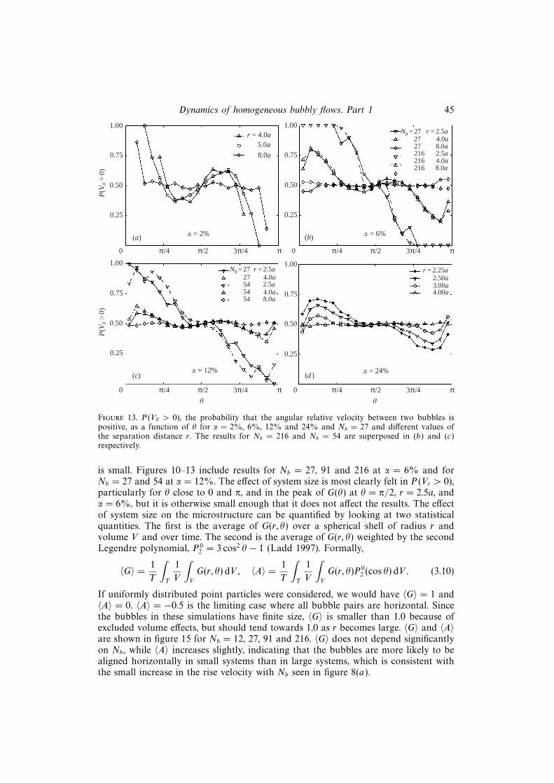
Dynamics of homogeneous bubbly flows. Part 1 45
π /40
(a) (b)α = 2%
1.00
P(V
õ>
0)
0.75
0.50
1.00Nb = 27 r = 2.5a
(c) (d )α = 12% α = 24%
õ
π /2 3π /4 π
r = 4.0a5.0a
8.0a
0.25
2727216216216
4.0a8.0a2.5a4.0a8.0a
α = 6%
Nb = 27 r = 2.5a27545454
4.0a2.5a4.0a8.0a
π /40 π /2 3π /4 π
π /40 π /2 3π /4 π π /40 π /2 3π /4 πõ
r = 2.25a
4.00a
0.75
0.50
0.25
0.75
0.50
1.00
0.25
1.00
P(V
õ>
0)
0.75
0.50
0.25
3.00a2.50a
Figure 13. P (Vθ > 0), the probability that the angular relative velocity between two bubbles ispositive, as a function of θ for α = 2%, 6%, 12% and 24% and Nb = 27 and different values ofthe separation distance r. The results for Nb = 216 and Nb = 54 are superposed in (b) and (c)respectively.
is small. Figures 10–13 include results for Nb = 27, 91 and 216 at α = 6% and forNb = 27 and 54 at α = 12%. The effect of system size is most clearly felt in P (Vr > 0),particularly for θ close to 0 and π, and in the peak of G(θ) at θ = π/2, r = 2.5a, andα = 6%, but it is otherwise small enough that it does not affect the results. The effectof system size on the microstructure can be quantified by looking at two statisticalquantities. The first is the average of G(r, θ) over a spherical shell of radius r andvolume V and over time. The second is the average of G(r, θ) weighted by the secondLegendre polynomial, P 0
2 = 3 cos2 θ − 1 (Ladd 1997). Formally,
〈G〉 =1
T
∫T
1
V
∫V
G(r, θ) dV , 〈A〉 =1
T
∫T
1
V
∫V
G(r, θ)P 02 (cos θ) dV . (3.10)
If uniformly distributed point particles were considered, we would have 〈G〉 = 1 and〈A〉 = 0. 〈A〉 = −0.5 is the limiting case where all bubble pairs are horizontal. Sincethe bubbles in these simulations have finite size, 〈G〉 is smaller than 1.0 because ofexcluded volume effects, but should tend towards 1.0 as r becomes large. 〈G〉 and 〈A〉are shown in figure 15 for Nb = 12, 27, 91 and 216. 〈G〉 does not depend significantlyon Nb, while 〈A〉 increases slightly, indicating that the bubbles are more likely to bealigned horizontally in small systems than in large systems, which is consistent withthe small increase in the rise velocity with Nb seen in figure 8(a).
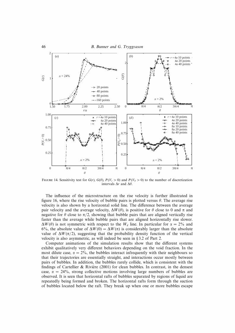
46 B. Bunner and G. Tryggvason
0
(a) (b)
α = 24%
2
G(r
)
2
r = 4a 10 points
(c) (d )
α = 2% α = 2%
õ
α = 2%
π /40 π /2 3π /4 π
π /40 π /2 3π /4 π π /40 π /2 3π /4 πõ
1
1.50
0.75
0.50
1.00
0.25
1.00
P(V
r>
0)
0.75
0.50
0.25
20 points40 points
80 points
160 points
4a 20 points4a 40 points
1.75 2.00 2.25 2.50
r = 4a 10 points4a 20 points4a 40 points8a 10 points8a 20 points8a 40 points
r/a õ
r = 4a 10 points4a 20 points4a 40 points
P(V
õ>
0)G
(õ)
Figure 14. Sensitivity test for G(r), G(θ), P (Vr > 0) and P (Vθ > 0) to the number of discretizationintervals ∆r and ∆θ.
The influence of the microstructure on the rise velocity is further illustrated infigure 16, where the rise velocity of bubble pairs is plotted versus θ. The average risevelocity is also shown by a horizontal solid line. The difference between the averagepair velocity and the average velocity, ∆W (θ), is positive for θ close to 0 and π andnegative for θ close to π/2, showing that bubble pairs that are aligned vertically risefaster than the average while bubble pairs that are aligned horizontally rise slower.∆W (θ) is not symmetric with respect to the Wd line. In particular for α = 2% and6%, the absolute value of ∆W (0) = ∆W (π) is considerably larger than the absolutevalue of ∆W (π/2), suggesting that the probability density function of the verticalvelocity is also asymmetric, as will indeed be seen in § 3.2 of Part 2.
Computer animations of the simulation results show that the different systemsexhibit qualitatively very different behaviors depending on the void fraction. In themost dilute case, α = 2%, the bubbles interact infrequently with their neighbours sothat their trajectories are essentially straight, and interactions occur mostly betweenpairs of bubbles. In addition, the bubbles rarely collide, which is consistent with thefindings of Cartellier & Riviere (2001) for clean bubbles. In contrast, in the densestcase, α = 24%, strong collective motions involving large numbers of bubbles areobserved. It is seen that horizontal rafts of bubbles separated by regions of liquid arerepeatedly being formed and broken. The horizontal rafts form through the suctionof bubbles located below the raft. They break up when one or more bubbles escape
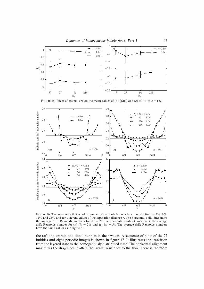
Dynamics of homogeneous bubbly flows. Part 1 47
0
(a) (b)0
r = 2.5a1
12 27 91 216Nb
0.8
0.6
0.4
0.2
r = 2.5a
⟨G ⟩
3.0a
6.0a
3.0a–0.1
–0.2
–0.3
–0.4
–0.5
–0.612 27 91 216
Nb
Figure 15. Effect of system size on the mean values of (a) 〈G(t)〉 and (b) 〈G(t)〉 at α = 6%.
(a) (b)α = 2%
29
Bub
ble
pair
dri
ft R
eyno
lds
num
ber
r = 4.0a
(c) (d )α = 12% α = 24%
õ
α = 6%
Nb = 27 r = 2.5a275454
4.0a2.5a4.0a
π /4 π /2 3π /4 π
π /40 π /2 3π /4 π π /40 π /2 3π /4 πõ
13
12
14
11
0
r = 2.10a2.50a
8.0a28
27
26
25π /4 π /2 3π /4 π0
30
28
26
24
22
20
18
24
Bub
ble
pair
dri
ft R
eyno
lds
num
ber
22
20
18
14
16
10
4.00a
Nb = 27 r = 2.5a
27
216
8.0a
2.5a
8.0a216
Figure 16. The average drift Reynolds number of two bubbles as a function of θ for α = 2%, 6%,12% and 24% and for different values of the separation distance r. The horizontal solid lines markthe average drift Reynolds numbers for Nb = 27, the horizontal dashdot lines mark the averagedrift Reynolds number for (b) Nb = 216 and (c) Nb = 54. The average drift Reynolds numbershave the same values as in figure 8.
the raft and entrain additional bubbles in their wakes. A sequence of plots of the 27bubbles and eight periodic images is shown in figure 17. It illustrates the transitionfrom the layered state to the homogenously distributed state. The horizontal alignmentmaximizes the drag since it offers the largest resistance to the flow. There is therefore
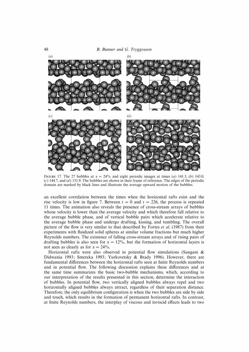
48 B. Bunner and G. Tryggvason
(a) (b)
(c) (d )
Figure 17. The 27 bubbles at α = 24% and eight periodic images at times (a) 141.3, (b) 143.0,(c) 144.7, and (d ) 151.9. The bubbles are shown in their frame of reference. The edges of the periodicdomain are marked by black lines and illustrate the average upward motion of the bubbles.
an excellent correlation between the times when the horizontal rafts exist and therise velocity is low in figure 7. Between t = 0 and t = 226, the process is repeated11 times. The animation also reveals the presence of cross-stream arrays of bubbleswhose velocity is lower than the average velocity and which therefore fall relative tothe average bubble phase, and of vertical bubble pairs which accelerate relative tothe average bubble phase and undergo drafting, kissing, and tumbling. The overallpicture of the flow is very similar to that described by Fortes et al. (1987) from theirexperiments with fluidized solid spheres at similar volume fractions but much higherReynolds numbers. The existence of falling cross-stream arrays and of rising pairs ofdrafting bubbles is also seen for α = 12%, but the formation of horizontal layers isnot seen as clearly as for α = 24%.
Horizontal rafts were also observed in potential flow simulations (Sangani &Didwania 1993; Smereka 1993; Yurkovetsky & Brady 1996). However, there arefundamental differences between the horizontal rafts seen at finite Reynolds numbersand in potential flow. The following discussion explains these differences and atthe same time summarizes the basic two-bubble mechanisms, which, according toour interpretation of the results presented in this section, determine the interactionof bubbles. In potential flow, two vertically aligned bubbles always repel and twohorizontally aligned bubbles always attract, regardless of their separation distance.Therefore, the only equilibrium configuration is when the two bubbles are side by sideand touch, which results in the formation of permanent horizontal rafts. In contrast,at finite Reynolds numbers, the interplay of viscous and inviscid effects leads to two
Dynamics of homogeneous bubbly flows. Part 1 49
equilibrium configurations, one vertical and unstable and the other horizontal andstable. When the separation between two vertically aligned bubbles is large, theyattract each other due to the wake effect until they reach an equilibrium separationdistance, where the potential effect balances the wake effect. This separation distanceincreases as Re increases (Yuan & Prosperetti 1994). For our value of Re, theseparation distance is approximately 2.6a, implying that vertically aligned bubblesusually attract each other. However, the vertical alignment is unstable. If disturbed,the two bubbles will rotate around each other and move to a horizontal alignment.In the horizontal alignment, the two bubbles attract each other when they are farfrom each other due to inviscid effects and repel each other when they are close dueto viscous effects (Legendre & Magnaudet 1998). The equilibrium separation distancedecreases when Re increases. The horizontal equilibrium is stable, which explainsthe preference for bubble pairs to be aligned horizontally and, for α = 24%, theformation of horizontal rafts. However, the horizontal rafts are only temporary. Dueto the attraction between vertically aligned bubbles, the rafts break up immediatelyafter they form.
4. ConclusionThe motion of buoyant bubbles in a homogeneous flow is studied by direct
numerical simulations, where the effects of viscosity, inertia, interface deformation,and surface tension are all accounted for. The bubbles can deform but remain nearlyspherical for the parameters used here. The rise Reynolds number is 12–30, dependingon the void fraction, which varies between 2% and 24%. This part focuses on the risevelocity and the microstructure of the bubbles; the dispersion process of the bubblesand the turbulence of the liquid phase are examined in Part 2. The major observationsand conclusions are as follows:
(i) A good estimate of the mean drift velocity of the bubbles can be achieved withonly 12 bubbles. Likewise, the effect of system size on the microstructure is smallwhen Nb > 12.
(ii) As the void fraction α increases, the drift velocity of the bubbles decreases from26.60 for α = 2% to 11.87 for α = 24%. In particular, there is a sharp drop betweenthe drift velocity at α = 0 and the drift velocity at α = 2%. A similar observationis made in the experimental study of van Wijngaarden & Kapteyn (1990) at higherReynolds numbers.
(iii) An analysis of the microstructure reveals a preference for pairs of bubbles tobe aligned horizontally. This is consistent with potential flow theory. However, thedynamics of bubble–bubble interactions are markedly different from potential flowpredictions. In our simulations, two bubbles that are aligned vertically attract eachother due to the wake effect, rotate around each other, and then repel when they arealigned horizontally. This mechanism is similar to the ‘drafting, kissing, and tumbling’mechanism of Fortes et al. (1987).
(iv) At α = 24%, we observe the periodic formation of horizontal rafts of bubblesseparated by liquid. These rafts are not stable and break up when one bubble leavesthe rafts and entrains other bubbles behind it. A similar phenomenon has been seenin the sedimentation of spheres in fluidized beds at the same packing fraction (Forteset al. 1987).
(v) While simulations of regular arrays do not provide any information on themicrostructure, they can be used to determine rough estimates of the average risevelocity of the bubbles at high void fractions.
50 B. Bunner and G. Tryggvason
The authors gratefully acknowledge the support of the National Science Foundationunder grant CTS-9503208 and of the University of Michigan through a RackhamPredoctoral Fellowship. This research was supported in part by NSF cooperativeagreement ACI-9619020 through computing resources provided by the NationalPartnership for Advanced Computational Infrastructure at the University of MichiganCenter for Parallel Computing. In addition, this research, in part conducted atthe Maui High Performance Computing Center, was sponsored in part by the AirForce Research Laboratory, Air Force Materiel Command, USAF, under cooperativeagreement number F29601-93-2-0001. The views and conclusions contained in thisdocument are those of the authors and should not be interpreted as necessarilyrepresenting the official policies or endorsements, either expressed or implied, of theAir Force Research Laboratory, the US Government, The University of New Mexico,or the Maui High Performance Computing Center.
REFERENCES
Bhaga, D. & Weber, M. E. 1981 Bubbles in viscous liquids: shapes, wakes, and velocities. J. FluidMech. 105, 61–85.
Biesheuvel, A. & van Wijngaarden, L. 1982 The motion of pairs of gas bubbles in a perfect fluid.J. Engng Maths 16, 349–365.
Bunner, B. & Tryggvason, G. 1999 A parallel front-tracking method for the simulation of dispersedmultiphase flows. In Proc. Ninth SIAM Conf. on Parallel Processing for Scientific Computing,San Antonio.
Bunner, B. 2000 Numerical simulation of gas-liquid bubbly flows. PhD Thesis, The University ofMichigan.
Bunner, B. & Tryggvason, G. 2002a Dynamics of homogeneous bubbly flows. Part 2: Velocityfluctuations. J. Fluid Mech. 466, 53–84.
Bunner, B. & Tryggvason, G. 2002b Effect of bubble deformation on the stability and propertiesof bubble flows. Submitted to J. Fluid Mech.
Cartellier, A. & Riviere, N. 2001 Bubble-induced agitation and microstructure in uniform bubblyflows at small to moderate particle Reynolds numbers. Phys. Fluids 13, 2165–2181.
Clift, R., Grace, J. R. & Weber, M. E. 1978 Bubbles, Drops, and Particles. Academic.
Delhaye, J. M. 1974 Jump Conditions and entropy sources in two-phase systems. Local instantformulation. Intl J. Multiphase Flow 1, 393–409.
Drew, D. A. 1983 Mathematical modeling of two-phase flow. Annu. Rev. Fluid Mech. 15, 261–291.
Duineveld, P. C. 1995 The rise velocity and shape of bubbles in pure water at high Reynoldsnumber. J. Fluid Mech. 292, 325–332.
Elghobashi, S. E. & Truesdell, G. C. 1992 Direct simulation of particle dispersion in decayingisotropic turbulence. J. Fluid Mech. 242, 655–700.
Esmaeeli, A. & Tryggvason, G. 1996 An inverse energy cascade in two-dimensional, low Reynolds-number bubbly flows. J. Fluid Mech. 314, 315–330.
Esmaeeli, A. & Tryggvason, G. 1998 Direct numerical simulations of bubbly flows. Part 1. LowReynolds number arrays. J. Fluid Mech. 377, 313–345.
Esmaeeli, A. & Tryggvason, G. 1999 Direct numerical simulations of bubbly flows. Part 2.Moderate Reynolds number arrays. J. Fluid Mech. 385, 325–358.
Fan, L. S. & Tsuchiya, K. 1990 Bubble Wake Dynamics in Liquids and Liquid Solid Suspensions.Butterworth-Heinemann.
Feng, J., Hu, H. H. & Joseph, D. D. 1994 Direct simulation of initial value problems for the motionof solid bodies in a Newtonian fluid. Part 1. Sedimentation. J. Fluid Mech. 261, 95–134.
Fortes, A. F., Joseph, D. D. & Lundgren, T. S. 1987 Nonlinear mechanics of fluidization of bedsof spherical particles. J. Fluid Mech. 177, 467–483.
Glowinski, R., Pan, T.-W., Hesla, T. I. & Joseph, D. D. 1999 A distributed Lagrange multi-plier/fictitious domain method for particulate flows. Intl J. Multiphase Flow 25, 755–794.
Harper, J. F. 1970 On bubbles rising in line at large Reynolds numbers. J. Fluid Mech. 41, 751–758.
Dynamics of homogeneous bubbly flows. Part 1 51
Hetsroni, G. 1982 Handbook of Multiphase Systems. McGraw Hill.
Ishii, M. 1975 Thermo-fluid Dynamic Theory of Two-phase Flows. Eyrolles.
Ishii, M., Chawla, T. C. & Zuber, N. 1976 Constitutive equation for vapor drift velocity intwo-phase annular flow. AIChE J. 22, 283–289.
Ishii, M. & Zuber, N. 1979 Drag coefficient and relative velocity in bubbly, droplet or particulateflows. AIChE J. 25, 843–855.
Jan, Y. J. 1994 Computational studies of bubble dynamics. PhD Thesis, The University of Michigan.
Katz, J. & Meneveau, C. 1996 Wake-induced relative motion of bubbles rising in line. Intl J.Multiphase Flow 22, 239–258.
Koch, D. L. & Ladd, A. J. C. 1997 Moderate Reynolds number flows through periodic and randomarrays of aligned cylinders. J. Fluid Mech. 349, 31–66.
Kok, J. B. W. 1989 Dynamics of gas bubbles moving through a liquid. Thesis, University of Twente.
Ladd, A. J. C. 1993 Dynamical simulations of sedimenting spheres. Phys. Fluids A 5, 299–310.
Ladd, A. J. C. 1997 Sedimentation of homogeneous suspensions of non-Brownian spheres. Phys.Fluids 9 (3), 491–499.
Lafaurie, B., Nardone, C., Scardovelli, R., Zaleski, S. & Zanetti, G. 1994 Modelling mergingand fragmentation in multiphase flows with SURFER. J. Comput. Phys. 113, 134–147.
Lamb, H. 1932. Hydrodynamics. Dover.
Legendre, D. & Magnaudet, J. 1998 Interaction between two spherical bubbles rising side by side.In Proc. Third Intl Conf. on Multiphase Flow, ICMF’98, Lyon, France.
Loewenberg, M. & Hinch, E. J. 1996 Numerical simulation of a concentrated emulsion in shearflow. J. Fluid Mech. 321, 395–419.
Maxworthy, T., Gnann, C., Kurten, M. & Durst, F. 1996 Experiments on the rise of air bubblesin clean viscous liquids J. Fluid Mech. 321, 421–441.
McLaughlin, J. B. 1996 Numerical simulation of bubble motion in water. J. Colloid Interface Sci.184, 614–625.
Nguyen, A. V. 1998 Prediction of bubble terminal velocities in contaminated water. AIChE J. 44,226–230.
Nobari, M. R., Jan, Y.-J. & Tryggvason, G. 1996 Head-on collision of drops – A numericalinvestigation. Phys. Fluids 8, 29–42.
Nott, P. R. & Brady, J. F. 1994 Pressure-driven flow of suspensions: simulations and theory.J. Fluid Mech. 275, 157–199.
Oka, H. & Ishii, K. 1999 Numerical analysis on the motion of gas bubbles using level set method.J. Phys. Soc. Japan 68, 823–832.
Peskin, C. S. 1977 Numerical analysis of blood flow in the heart. J. Comput. Phys. 25, 220.
Pozrikidis, C. 1993 On the transient motion of ordered suspensions of liquid drops. J. Fluid Mech.246, 301–320.
Qian, J. 1997 Droplet and flame dynamics in combustion phenomena. PhD Thesis, PrincetonUniversity.
Ryskin, G. & Leal, L. G. 1984 Numerical solution of free-boundary problems in fluid mechanics.Part 2. Buoyancy-driven motion of a gas bubble through a quiescent liquid. J. Fluid Mech.148, 19–35.
Saffman, P. G. 1973 On the settling speed of free and fixed suspensions. Stud. Appl. Maths LII,115–127.
Sangani, A. S., Zhang, D. Z. & Prosperetti, A. 1991 The added mass, Basset, and viscous dragcoefficients in nondilute bubbly liquids undergoing small-amplitude oscillatory motion. Phys.Fluids A 3, 2955–2970.
Sangani, A. S. & Didwania, A. K. 1993 Dynamic simulations of flows of bubbly liquids at largeReynolds numbers. J. Fluid Mech. 250, 307–337.
Smereka, P. 1993 On the motion of bubbles in a periodic box. J. Fluid Mech. 254, 79–112.
Spelt, P. D. M. & Sangani, A. S. 1998 Properties and averaged equations for flows of bubblyliquids. Appl. Sci. Res. 58, 337–386.
Squires, K. D. & Eaton, J. K. 1990 Particle response and turbulence modification in isotropicturbulence. Phys. Fluids A 2, 1191–1203.
Tryggvason, G., Bunner, B., Esmaeeli, A., Juric, D., Al-Rawahi, N., Tauber, W., Han, J., Nas, S.
52 B. Bunner and G. Tryggvason
& Jan, Y.-J. 2001 A front tracking method for the computations of multiphase flow. J. Comput.Phys. 169, 708–759.
Unverdi, S. O. & Tryggvason, G. 1992 A front-tracking method for viscous, incompressible,multi-fluid flows. J. Comput. Phys. 100, 25–37.
Wang, L.-P. & Maxey, M. R. 1993 Settling velocity and concentration distribution of heavy particlesin homogeneous isotropic turbulence. J. Fluid Mech. 256, 27–68.
van Wijngaarden, L. 1993 The mean rise velocity of pairwise-interacting bubbles in liquid. J. FluidMech. 251, 55–78.
van Wijngaarden, L. & Kapteyn, C. 1990 Concentration waves in dilute bubble/liquid mixtures.J. Fluid Mech. 212, 111–137.
Yuan, H. & Prosperetti, A. 1994 On the in-line motion of two spherical bubbles in a viscous fluid.J. Fluid Mech. 278, 325–349.
Yurkovetsky, Y. & Brady, J. 1996 Statistical mechanics of bubbly liquids. Phys. Fluids 8, 881–895.
Zenit, R., Koch, D. L., & Sangani, A. S. 2001 Measurements of the average properties of asuspension of bubbles rising in a vertical channel. J. Fluid Mech. 429, 307–341.
Zhou, H. & Pozrikidis, C. 1993 The flow of ordered and random suspensions of two-dimensionaldrops in a channel. J. Fluid Mech. 255, 103–127.
Copyright © 2022 FDOKUMEN