
Dynamics of Electricity Consumption, Oil Price and Economic ...
54
Munich Personal RePEc Archive Dynamics of Electricity Consumption, Oil Price and Economic Growth: Global Perspective Muhammad, Shahbaz and Sarwar, Suleman and Wei, Chen and Malik, Muhammad Nasir Montpellier Business School, Montpellier, France, School of Economics, Shandong University, Jinan, China, UCP Business School, University of Central Punjab Lahore, Pakistan 1 May 2017 Online at https://mpra.ub.uni-muenchen.de/79532/ MPRA Paper No. 79532, posted 06 Jun 2017 04:45 UTC
-
Upload
khangminh22 -
Category
Documents
-
view
1 -
download
0
Transcript of Dynamics of Electricity Consumption, Oil Price and Economic ...

Munich Personal RePEc Archive
Dynamics of Electricity Consumption,
Oil Price and Economic Growth: Global
Perspective
Muhammad, Shahbaz and Sarwar, Suleman and Wei, Chen
and Malik, Muhammad Nasir
Montpellier Business School, Montpellier, France, School of
Economics, Shandong University, Jinan, China, UCP Business
School, University of Central Punjab Lahore, Pakistan
1 May 2017
Online at https://mpra.ub.uni-muenchen.de/79532/
MPRA Paper No. 79532, posted 06 Jun 2017 04:45 UTC

1
Dynamics of Electricity Consumption, Oil Price and Economic Growth: Global Perspective
Muhammad Shahbaz
Energy and Sustainable Development Montpellier Business School, Montpellier, France.
Email: [email protected]
Suleman Sarwar
School of Economics, Shandong University, Jinan, China Email: [email protected]
Chen Wei
School of Economics, Shandong University, Jinan, China. Email: [email protected]
Muhammad Nasir Malik
UCP Business School, University of Central Punjab Lahore, Pakistan. Email: [email protected]
Abstract: This study uses the data from 157 countries from 1960 to 2014 to analyze the relationship between economic growth, electricity consumption, oil prices, capital, and labor. The economic growth of developing countries with industrial infrastructure has a more significant association with electricity consumption than oil prices. We use oil prices and electricity consumption jointly to study highly predictive observations for economic growth. The data are categorized by income, OECD and regional levels. The panel cointegration, long-run parameter estimation, and Pool Mean Group testsare used to analyze the cointegration and short-run and long-run relationships between the variables. The empirical results indicate the presence of cointegration between the variables. The presence of feedback effects between electricity consumption and economic growth, oil prices and economic growth is valid. These findings confirm that inspite of the oil prices, developing countries rely heavily on electricity consumption for economic growth. In the short run, growth and feedback effects suggest that more vigorous electricity policies should be implemented to attain sustainable economic growth for the long-term. Keywords: Electricity Consumption, Oil Prices, GDP, Capital, Population JEL Classification: Q43, Q48, O13

2
1. Introduction
The economic progress of developing countries relies heavily on electricity. The production
of manufacturing industries declines due to electricity shortages, which, in turn, destabilize
an economy. Electricity consumption is a key component of economic growthand is directly
or indirectly a complement to labor and capital as a factor of production (Costantini and
Martini, 2010). Various studies have revealed the diverse impact of electricity consumption
on economic growth (Yuan et al. 2007, Chen et al. 2007, Yuan et al. 2008, Narayan and
Prasad 2008, Abosedra et al. 2009, Mutascu 2016, Ahmed and Azam 2016, Streimikiene and
Kasperowicz 2016). For example, some studies suggest apositive impact of electricity
consumption on economic growth (Shiu and Lam 2004, Yuan et al. 2007, Shahbaz and Lean
2012, Iyke 2015, Tang et al. 2016, Streimikiene and Kasperowicz 2016). Ozturk (2010)
argues that if economic growth is inversely affected by energy consumption, then different
arguments could justify the adverse impacts of energy consumption on economic growth. For
example, we could imagine a situation in which a growing economy aims to reduce the level
of energy consumption through production shifts to less energy-intensive sectors.
Furthermore, the inefficient use of energy, such as constraints in capacity use or an inefficient
supply of energy, may also have a negative impact on economic growth or growth in real
GDP (Chontanawat et al. 2008, Payne 2010, Ozturk 2010). A large number of developing
countries have concerns about electricity shortagesdue to scarce resources and infrastructure
(Allcott et al. 2014, Shahbaz and Ali 2016). The relationship between electricity consumption
and economic growth also varies across the income levels of countries (Yoo and Kwak,
2010). Similarly, Ferguson et al. (2000) reported that the relationship between electricity
consumption and economic growth is stronger in high-income countries.

3
Oil prices are a key component of energy, and their importance in economic development has
been recognized by economists, policy makers, businessmen, households, and researchers.
After the 1973 oil crisis, several studies (Timilsina 2015, Kilian and Vigfusson 2011, Kilian
2008, Hamilton 1983, 1985, Gisser and Goodwin 1986, Mork 1989) affirmed an inverse
relationship between oil prices and economic growth. Economists and researchers have
reached a consensus that oil price volatility simultaneously reduces economic growth.
However, the recent literature shows the negative relationship decreasing over time because
of oil alternatives and preemptive governmental measures against sudden oil price shocks
(Doroodian and Boyd 2003, Jbir and Zouari-Ghorbel 2009). Oil-importing developing
economies are severely affected by oil price hikes because of a lower tax share on oil prices.
Moreover, developed economies have a higher tax share on oil. Therefore, such oil price
shocks may be mitigated to an extent by suspending the tax share as oil prices rise.
Developing countries with less of a tax share on oil have less ability to absorb oil price
shocks. Consequently, oil price hikes appear to have a more adverse impact on developing
economies.
These dynamics between electricity consumption, oil prices and economic growth prompt
researchers to conduct empirical research and provide diverse empirical evidence. This paper
is a humble effort to provide comprehensive empirical evidence by covering data from 157
countries for the period from 1960 to 2014. This study contributes tothe existing energy
literature in four ways: (i) The study employs the growth model developed by Solow (1956)
by augmenting the production function to investigate the role of electricity consumption and
oil prices on domestic production. The industrial infrastructure heavily relies on oil as an
input to production operations and transportation. The increase in oil prices leads to higher
costs of production and drives inflation, which adversely affects investment and purchasing

4
power. Electricity supply is the basic element of industrial production, and countries facing
an electricity shortage cannot sustain the pace of economic growth. The economic growth of
developing countries with industrial infrastructure has a high and significant association with
electricity consumption compared to oil prices. The production process can be slowed due to
an electricity shortage (Shahbaz and Ali 2016). Such a decline in output has a direct influence
on financial values. On the other hand, to mitigate such massive losses, many firms attempt to
acquire alternative energy-producing plants, which also escalate production costs. The
increase in electricity consumption in manufacturing economies may help to trigger
economic growth (Kahane and Squitieri 1987). Therefore, this study has incorporated
electricity consumption as a factor of domestic production along with oil prices in an
augmented production function. The joint use of electricity consumption and oil prices in the
augmented production function will also provide new guidelinesfor policy makers to design
comprehensive growth policies while considering the role of electricity consumption and oil
prices. The ignorance of relevant variables in the function of production may be a reason for
the ambiguous results of previous studies in the existing literature (Shahbaz et al. 2016). (ii)
The paper investigates the electricity-growth nexus using data from 157 countries, which are
further categorized into sub-panels, such as regional, income, OECD and non-OECD levels,
to mitigate heterogeneity in the data. (iii) This study applies the panel cointegration approach
developed by Westerlund (2007). The Fully Modified Ordinary Least Square (FMOLS) and
Pool Mean Group (PMG) tests have also been applied to scrutinize the short-run and long-run
associations between the variables. (iv) The heterogeneous panel causality test originated by
Dumitrescu and Hurlin (2012) is used to examine the causality relationship between
electricity consumption and economic growth in heterogeneous panels. Our results show the
existence of a feedback effect between electricity consumption and economic growth. The
association between oil prices and economic growth is also bidirectional. Gross fixed capital
5
formation and labor lead to economic growth. The findings show heavy reliance by
developing countries on electricity consumption rather than oil prices for sustainable
economic growth. This finding varies across income levels and regions.
The rest of the study is organized as follows: Section 2 provides a brief literature review of
energy consumption, electricity consumption, oil prices and Pedroni panel cointegration.
Section 3 discusses the data and methodology used for estimations. Section 4 reports the
results and conclusion. Section 5 provides concluding remarks.
2.Literature Review
We have divided the literature review into two portions: (i) electricity consumption-economic
growth nexus and (ii) oil price-economic growth nexus.
2.1. Electricity Consumption and Economic Growth1
Researchers and academics have researched the energy-growth nexus using time series and
panel data sets but have reported conflicting empirical findings (Ozturk, 2010). These
discrepancies may not help policy makers in designing comprehensive economic and energy
policies touse electricity consumption as an economic tool to sustain economic growth in
thelongrun (Payne, 2010)2. For example, Murray and Nan (1996) applied the causality test
1A summary of electricity consumption-economic growth is given in Table-A1 (see Appendix) 2The existing literature on electricity consumption and the economic growth relationship provides four conflicting hypotheses: (i) The feedback effect reveals that electricity consumption causes economic growth and that economic growth causes electricity consumption. This hypothesis is empirically validated by Masih and Masih (1996), Constantini and Martini (2010), Shahbaz et al. (2012), Polemis and Dagoumas (2013), Mutascu (2016) and Sarwar et al. (2017). The feedback effect indicates that a decline in the electricity supply impedes economic growth and a reduction in economic growth will decrease electricity demand (ii) The growth hypothesis validates the presence of unidirectional causality running from electricity consumption to economic growth. This indicates that electricity consumption plays a vital role in enhancing domestic production and, hence, economic growth. Empirically, the growth hypothesis is empirically confirmed by Murry and Nan (1994), Khan et al. (2007), Pradhan (2010), Das et al. (2012), Tang and Shahbaz (2013), Wolde-Rufael (2014), Iyke (2015) and He et al. (2017). The feedback and growth hypothesis reveals the importance of energy-

6
developed by Granger (1969) to examine the relationship between electricity consumption
and economic growth using data from 15 countries from 1970 to 1990. They found neutral
effects between both variables in the cases of India, the Philippines, and Zambia.
Furthermore, their analysis indicates that the conservation hypothesis is valid for Colombia,
ElSalvador, Indonesia, and Kenya, whereas the growth effect is found in Mexico, Canada,
Hong Kong, Pakistan, Singapore, Turkey, Malaysia, and South Korea. Wolde-Rufael (2006)
applied the bounds testing approach developed by Pesaran et al. (2001) as well as the
causality developed by Toda and Yamamoto (1995) to examine cointegration and causality
between electricity consumption and economic growth in 17 African countries. The results
reveal that economic growth causes electricity consumption in 6 countries (Cameroon,
Ghana, Nigeria, Senegal, Zambia, Zimbabwe), whereas electricity consumption causes
economic growth in 3 countries (Benin, Republic of Congo, Tunisia), and the feedback effect
exists between both variables in 3 countries (Egypt, Gabon, Morocco)3. Yoo (2006)
investigated the direction ofthe causal association between electricity consumption and
economic growth for ASEAN countries and reported a feedback effect for Malaysia and
Singapore and that economic growth causes electricity consumption in Indonesia and
Thailand. In the case of the OPEC region, Squalli (2007) employed the bounds testing and
causality approaches developed by Pesaran et al. (2001) and Toda and Yamamoto (1995),
respectively, to examine cointegration and causality between electricity consumption and
economic growth. The causality results indicate the dependence of economic growth on
(electricity) exploring policies to attain long-run economic growth. (iii) The conservation hypothesis reveals that unidirectional causality runs from economic growth to electricity consumption. This shows that electricity consumption does not play a vital role in stimulating economic growth. The conservation hypothesis is empirically validated by Cheng and Lai (1997), Aqeel and Butt (2001), Narayan and Singh (2007), Narayan et al. (2010), Mahmoodi and Mahmoodi (2011), Shahbaz and Feridun (2012) and Kasnan and Dunan (2015). (iv) The neutral effect indicates that electricity consumption does not lead economic growth and vice versa. This hypothesis is empirically confirmed by Yu and Hwang (1984), Chontanawat et al. (2008), Wolde-Rufael (2009) and Smiech and Papiez (2014).The conservation and neutral hypotheses reveal minor (or no) role of electricity consumption in promoting economic growth. In such circumstances, energy (electricity) conservation policies are suitable because they have no adverse effect on economic growth.
3 A neutral effect also exists in the cases of Algeria, PR Congo, Kenya, South Africa, and Sudan.

7
electricity consumption. Chen et al. (2007) investigated the association between electricity
consumption and economic growth in 10 industrialized countries from 1971to 2001. Their
analysis showedthat electricity consumption causes economic growth, and as a result,
economic growth causes electricity consumption.Narayana and Singh (2007) applied the
multivariate production function by incorporating labor as an additional determinant of
economic growth and electricity consumption for the Fiji Islands for the period from 1971 to
2002. Their results show the presence of unidirectional causality from economic growth and
labor to electricity consumption4.
Using data from 30 OECD countries, Narayan and Prasad (2008) used the bootstrap causality
test to examine the causal relationship between electricity consumption and economic
growth. They suggested that the implementation of energy conservation policies is not
harmful to economic growth. Ciarreta and Zarraga (2008) investigated the causal association
between electricity consumption and economic growth in European economies by applying
panel cointegration and causality approaches. They found that electricity consumption
predicts economic growth in the long run. Oztuek and Acaravci (2010) investigated the
4Cheng and Lai (1997) applied Hsiao’s version of the Granger causality for Taiwan for the period from 1955 to 1993. Their results indicated the presence of unidirectional causality from economic growth to energy consumption. Asafu-Adjaye (2000) noted that energy consumption caused economic growth for India and Indonesia for the 1973-1995 period. By contrast, in Thailand and the Philippines, a feedback effect was noted between energy consumption and economic growth over the period from 1971 to 1995. Soytas and Sari (2003) used the data from G-7 and 10 emerging economies, but not PR China, for the period from 1950 to 1990 to examine the association between energy consumption and economic growth. They reported that energy consumption has a positive and significant effect on economic growth in Argentina, Italy and Korea and that unidirectional causality from economic growth to energy consumption also exists. Ghali and El-Sakka (2004) collected Canadian data for the period from 1961 to1997 to examine linkages between energy consumption and economics by applying the Johansen-Juselius (1990) and variance decomposition approaches. They confirmed the presence of bidirectional causality between energy consumption and economic growth. Mehrara (2007) attempted to investigate the relationship between energy consumption and economic growth for 11 oil-exporting countries over the period from 1971 to 2002 and found a positive impact of economic growth on energy consumption. Erdal, Erdal and Esengün (2008) also reported bidirectional causality between economic growth and energy consumption for the Turkish economy. Lee et al. (2008) studied the relationship between energy consumption and economic growth for 22 OECD countries by applying the Pedroni panel cointegration test. Their findings supported the presence of a feedback effect between energy consumption per capita and real GDP per capita. Bartleet and Gounder (2010) reported that economic growth stimulated energy consumption in New Zealand.

8
relationship between electricity consumption and economic growth in the cases of 15
transition economies using panel cointegration and causality approaches5. Their analysis
indicated no cointegration between the variables and that the implementation of energy
(electricity) conservation policies would affect economic growth.
Yoo and Kwak (2010) empirically examined the relationship between electricity consumption
and economic growth using data from 7 South American countries for the period from 1975
to 2006. Their results showed that economic growth is the Granger cause of electricity
consumption in Ecuador, Columbia, Chile, Brazil and Argentina, but a feedback effect also
exists for Venezuela, whereas a neutral effect is valid for Peru. Apergis and Payne (2011)
used a multivariate production function using a panel of 88 countries to examine the
association between electricity consumption and economic growth. They used a panel error
correction model and found a feedback effect between electricity consumption and economic
growth for high-income and upper-middle-income country panels, whereas electricity
consumption causes economic growth in the lower income country panel. Das et al. (2012)
used data from 45 countries from 1971 to 2009 by applying the generalized method of
moments (system GMMs) test developed by Blundell and Bond (1998) to examine the
linkage between electricity consumption and economic growth. They found a positive and
significant association between both variables.
Wolde-Rufael (2014) investigated the relationship between electricity consumption and
economic growth for 15 transition countries by applyinga bootstrap panel cointegration test.
The results indicated that electricity consumption significantly affects economic growth in
5Albania, Belarus, Bulgaria, Czech Republic, Estonia, Latvia,Lithuania, Macedonia, Moldova, Poland,
Romania, Russian Federation, Serbia, Slovak Republic and Ukraine.

9
Bulgaria and Belarus; that economic growth causes energy consumption in the Czech
Republic, Lithuania, Latvia; and that a feedback effect is valid for the Russian Federation and
Ukraine. Similarly, Karanfil and Li(2015) investigated the relationship between electricity
consumption and economic growth for 160 countries from 1980 to 2012. They reported that
electricity consumption and economic growth relationship is sensitive to regional differences,
income levels, urbanization levels and supply risks as well. Abdoli and Dastan (2015)
examined the association between electricity consumption and economic growth by
incorporating exports as a potential determinant of the production function for OPEC
countries. They employed fully modified OLS (FMOLS) and found that electricity
consumption and trade stimulate economic growth. Their causality analysis reveals the
presence of a feedback effect between electricity consumption and economic growth in the
short run. Kayikci and Bildirici (2015) applied the bounds testing approach to examine the
relationship between economic growth, electricity consumption and oil rents for the GCC and
MENA regions. They noted that the causality relationship with electricity consumption
depends upon natural resource levels.
Osman et al. (2016) applied PMGE and demeaned the PMG, AMG, MGE and DFE
approaches to investigate the association between electricity consumption and economic
growth in the case of GCC countries. They found that electricity consumption and
capitalization spur economic growth. Their analysis indicates the presence of a feedback
effect between electricity consumption and economic growth. However, unidirectional
causality is noted from capitalization to electricity consumption, whereas economic growth
causes capitalization.

10
2.2. Oil Price and Economic Growth
The general perception about the correlation between oil price and GDP is that a decline in
the prices of crude oil decreases inflation (Maeda, 2008). In fact, it is also responsible for the
petroleum subsidy along with the interest rates and fiscal deficit; this increases the GDP
growth rate and promotes economic development in the country. The relationship between oil
price and economic growth was explored by Morey (1993) for the US economy. The
empirical results show that oil price hikes decrease economic activity and hence economic
growth. Later, Jimenez-Rodriguez and Sanchez (2005) collected data for OECD countries to
examine the impact of oil price on economic growth. They found that oil price shocks
positively and negatively affect economic growth in oil-exporting and oil-importing
countries. Lardic and Mignon (2006) investigated the asymmetric relationship between oil
price and economic growth by applying asymmetric cointegration. They found that
cointegration exists between the variables and that an oil price increase impedes economic
growth. Mehrara (2008) analyzed the relationship between oil price and economic growth for
oil-exporting economies. The empirical evidence reported that the relationship between oil
price and GDP is non-linear and asymmetric. Farzanegan and Markwardt (2009) investigated
the relationship between oil price and macroeconomic variables for Iran. Their results
confirmed that a positive shock in oil price has a significant and positive impact on industrial
production. In contrast, negative shocks in oil prices have an adverse impact on industrial
production. Jayaraman and Choong (2009) attempted to investigate the association between
oil price and economic growth in oil-importing economies. Their empirical data reveal that
oil price has a negative and significant effect on economic growth and the unidirectional
causality exists running from oil price to economic growth. Ozlale and Pekkurnaz (2010)
analyzed the linkages between oil price and macroeconomic variables for the Turkish

11
economy. They applied a structural vector autoregression model (SVAR) and confirmed that
oil price leadsto a current account deficit that leads to a decline in economic growth. In the
case of China, Tang et al. (2010) reported that oil price shocks adversely affect economic
growth and investment.
Using data from the G-7, OPEC economies, Russia, India and China, Ghalayini (2011)
reinvestigated the association between oil price shocks and economic growth. The empirical
exercise reveals that oil priceis negatively (positively) linked with economic growth in oil-
importing (exporting) countries. Timilsina (2015) studied 25 economies to examine the
empirical relationship between oil price and GDP. The results from the developing countries
reported a negative and significant effect of oil price on GDP. The main cause for this
negative relationship is the dependence of industries on oil. Moreover, the findings confirm
that the increase in oil price helps to strengthen the economy for oil-exporting countries. Ftiti
et al. (2016) examined the interdependence between oil price and economic growth using
(selected) OPEC countries’ monthly data for 2000-2010. They noted that oil price shocks
affect the oil-growth nexus in global business cycle fluctuations and the financial crisis
turmoil in the OPEC region. Sarwar et al. (2017) investigated 210 countries; they used the
findings to show that oil price has a significant effect on economic growth in the short and
long run.
3. The Model and Data
This study investigates the association between electricity consumption and economic growth
by incorporating oil price in the augmented production function. We have included oil
pricevariable into the production function due to its vital impact on economic activity. The
impact of oil price hikes is sensitive in oil-exporting and oil-importing countries. Oil prices
12
hike affect real economic activity via supply and demand channels and vice versa. The
supply-side channel reveals that oil is a basic factor for production, and an increase in oil
price lead to increase in the cost of production, which leads firms or industries to lower
output (Morey 1993, Tang et al. 2010). The demand-side channel entails that oil price shocks
affect not only consumption but also investment activities. Increase in oil prices will lower
output, which lowers real wages due to the decline in demand for labor as a result of the
decline in economic growth. A decline in economic growth is positively linked with less
disposable income and consumption as well (Maeda 2008, Tang et al. 2010, Ftiti et al. 2016).
Oil price hikes increase firms’ costs, the result of which decreases investment activities.
Indirectly, oil price shocks influence not only exchange rate but also inflation, which in turn
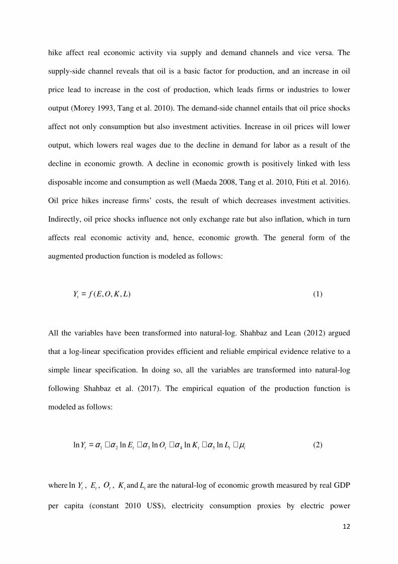
affects real economic activity and, hence, economic growth. The general form of the
augmented production function is modeled as follows:
),,,( LKOEfYt = (1)
All the variables have been transformed into natural-log. Shahbaz and Lean (2012) argued
that a log-linear specification provides efficient and reliable empirical evidence relative to a
simple linear specification. In doing so, all the variables are transformed into natural-log
following Shahbaz et al. (2017). The empirical equation of the production function is
modeled as follows:
ittttt LKOEY µααααα +++++= lnlnlnlnln 54321 (2)
where ln tY , tE , tO , tK and tL are the natural-log of economic growth measured by real GDP
per capita (constant 2010 US$), electricity consumption proxies by electric power
13
consumption per capita (KWh), oil price, capitalization measured by gross fixed capital
formation per capita (constant 2010 US$) and labor force per capita, respectively. iµ is an
error term with a normal distribution.
This study uses unbalanced panel data for 157 countries6 over the period from 1960 to 2014.
The data for the real gross domestic product (constant 2010 US$), electric power
consumption (KWh), real gross fixed capital formation (constant 2010 US$) and total labor
(population aged 15-64) were collected from World Development Indicators (CD-ROM,
2015)7. Crude oil price data are obtained from the Statistical Review of World Energy
(http://www.bp.com/en/global/corporate/about-bp/energy-economics/statistical-review-of-world-
energy.html). The total population is used to convert all variables into per capita units except
crude oil price.
3.1. Estimation Strategy
3.1.1. Cross-Sectional Dependence Test
Considering the globalization of the world economy, cross-sectional dependence may largely
exist among countries and regional economies. However, cross-sectional dependency is an
important factor that influences the result of panel unit root testing and cointegration testing.
In doing so, we have applied first- and second-unit root and cointegration tests. The first-
generation unit root and cointegration tests assumecross-sectional independence. The second-
generation unit root and cointegration tests consider cross-sectional dependence. To decide
which type of unit root and cointegration test is suitable, we test the null hypothesis of cross-
sectional independence. Using the seemingly unrelated regression equation (SURE), Breusch
6Initially we used data for 210 countries. The countries with unavailable GDP data since 1960 are excluded. 7 http://data.worldbank.org/

14
and Pagan (1980) proposed the Lagrange multiplier (LM) test, which is based on the average
of squared pair-wise correlations of the residuals. The empirical equation of the LM cross-
sectional dependence test is formulated as follows:
2
1
1
1 ij
N
ij
N
ilm STCD +=−
== αα (3)
where ijS is the sample estimate of the pair-wise correlation of residuals and is defined as
follows:
2/12
1
2/12
1
1
)()( jt
T
tit
T
t
jtit
T
t
jiijee
eeSS
==
===αα
α (4)
where ite is the Ordinary Least Squares (OLS) estimate of itµ , defined as follows:
itiiitit xbye −−= α (5)
Where t = 1……T and i= 1……N index the time-series and cross-sectional units,
respectively. However, the Breusch and Pagan (1980) LM test is likely to exhibit size
distortions when large N and small T exist, as in our data. Recognizing their shortcoming,
Pesaran (2004) proposed simple tests of error in cross-section dependence thatare applied to a
variety of panel data models. These tests include stationary and unit root dynamic
heterogeneous panels with short T and large N and are robust to single and even multiple
structural breaks in the slope coefficients and error variances of the individual regressions.
His cross-sectional dependence statistic is based on pair-wise correlation coefficients rather
than their squares, as used in the LM test:
15
21
1
1
1)1(
2ij
N
ij
N
i SNN
TCD
−+=
−=−
= αα (6)
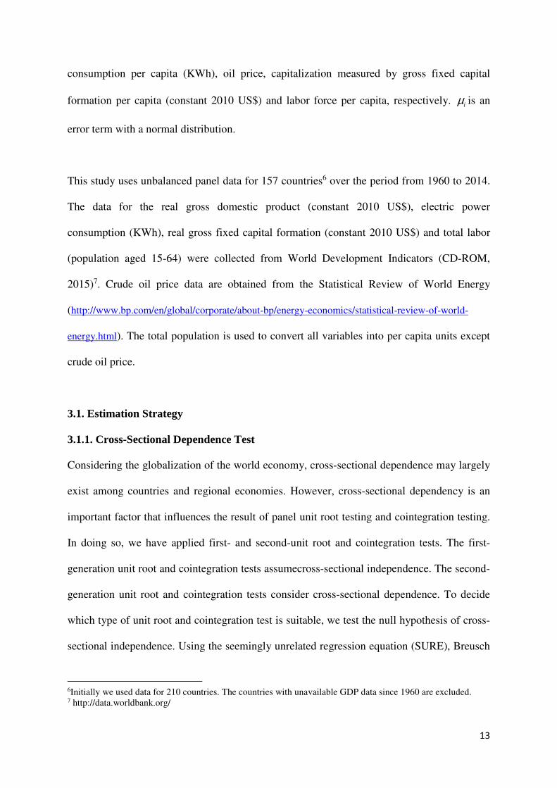
3.1.2.Panel Unit Root under Cross-Sectional Dependence
We apply the second-generation panel unit root test to examine the cross-sectional
dependence developed by Pesaran (2007). The Pesaran panel unit root uses the cross-section
mean to proxy the common factorand constructs the test statistics based on t-ratio of the OLS
estimate of )ˆ( ii bb in the following cross-sectional augmented DF (CADF) regression:
ittititiiiit eDydycybDy ++++= −− 11,α (7)
One possibility would be to consider a cross-sectional augmented version of the IPS testbased
on the formula given below:
),(),( 1
1TNtaNbartTNCIPS i
N
i=−=−= (8)
where ),( TNti is the augmented Dicky-Fuller statistic across the cross-section for the ith
cross-section unit set by the t-ratio of the coefficient ( 1, −ty i ) in the CADF regression.
3.1.3.Panel Cointegration Test
We apply the panel cointegration approach developed by Westerlund (2007), which generates
samples through the bootstrap approach and usesa new sample to construct a two-group mean
and two-panel statistics. This approach examines whether the model has an error correction
(full panel or individual groups) based on the model as follows:
16
itjitij
p
jjitij
p
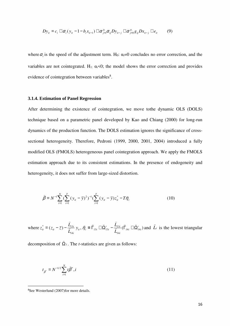
jitiitiiit eDxgDyxbycDy ii +++−−+= −=−=− 011)1( αααα (9)
where iα is the speed of the adjustment term. H0: αi=0 concludes no error correction, and the
variables are not cointegrated. H1: αi<0; the model shows the error correction and provides
evidence of cointegration between variables8.
3.1.4. Estimation of Panel Regression
After determining the existence of cointegration, we move tothe dynamic OLS (DOLS)
technique based on a parametric panel developed by Kao and Chiang (2000) for long-run
dynamics of the production function. The DOLS estimation ignores the significance of cross-
sectional heterogeneity. Therefore, Pedroni (1999, 2000, 2001, 2004) introduced a fully
modified OLS (FMOLS) heterogeneous panel cointegration approach. We apply the FMOLS
estimation approach due to its consistent estimations. In the presence of endogeneity and
heterogeneity, it does not suffer from large-sized distortion.
∑ ∑ ∑= = =
−− −−−=N
i
T
t
T
t
iititit TzyyyyN1 1 1
*121 )(())(( ηβ )) (10)
where )(,)( 1414
14
131313
14
13* oo))
)
))))
)
)
ii
i
iiiiit
i
iitit
L
Ly
L
Lzzz Ω+Γ−Ω+Γ≡−−= η and iL
) is the lowest triangular
decomposition of iΩ)
. The t-statistics are given as follows:
∑=
−=N
i
itNt1
*2/1 ,* ββ
))
(11)
8See Westerlund (2007)for more details.

17
where
2/1
1
21
130
** )()(,
−Ω−= ∑=
−T
t
itii yyit)))
βββ
3.1.5.Pool Mean Group (PMG) Test
We apply the Pool Mean Group (PMG) developed by Pesaran et al. (1999), which adopts a
parametric model to estimate the cointegration vector based on an error correction model in
which short-run dynamics are influenced by the deviation from the equilibrium. The
autoregressive distributive lag (ARDL) (p,q1,..,qk) dynamic panel specification is modeled as
follows:
it
P
j
ijtiijtiijit yxx εµδλ∑ ∑=
−− +++=1
,1, (12)
whereyi, t-j is the (k x 1) vector of explanatory variables for group i, and ui presents the fixed
effects. p and q can vary across countries, and the model is known as vector error correction
model (VECM):
tii
q
j
jtiij
p
j
jtiijtiitiit yxxxx ,
1
1
,
'1
1
,1,
'
1, )(( εµγγβθ ++∆+∆+−=∆ ∑∑−
=−
−
=−−− (13)
Whereβ ’i represents the long-run parameters and θi is the error correction term. The PMG
uses β’i, which is common across countries.
tii
q
j
jtiij
p
j
jtiijtitiit yxxxx ,
1
1
,
'1
1
,1,
'
1, )(( εµγγβθ ++∆+∆+−=∆ ∑∑−
=−
−
=−−− (14)
where β’ is the error correction speed of adjustment.

18
itit
i
iit xx π
βθ +−= )( (15)
where itπ presents the stationary process. If β’=0, the results do not confirm any long-run
relationship, and β’<0 confirmsalong-run relationship between variables. The PMG test is
intermediate between Mean Group (MG) estimations — in which slopes and coefficients are
permitted to differ across countries —and the fixed effect method (FEM) — in which
interceptsmay vary but slopes are fixed. In contrast, the PMG technique allows the
coefficients to vary across countries in the short run. Furthermore, the MG that averages the
coefficients of the country-specific regressions is also a consistent technique but is not a
better estimator when either the number of countries orthe period is small (Hsiao et al. 1999).
In comparison, the pool mean group estimator uses the combination of pooling and averaging
of coefficients.
3.1.6.Heterogeneous Panel Causality Test
To test causality, we use the Dumitrescu and Hurlin (2012) panel causality test. It is a
simplified version of the Granger (1969) non-causality test that is generally used for
heterogeneous panel data models with fixed coefficients. It considers the two dimensions of
heterogeneity: a) the heterogeneity of the regression model for testing the Granger causality
and b) the heterogeneity of the causality relationships. The linear model is as follows:
it
M
m
kti
m
i
M
m
mti
m
iiit yzz εβγα ∑∑=
−=
− +++=1
,
)(
1
,
)( (16)

19
Equation-16 shows that y and z are two stationary variables for a number of individuals (N)
in time periods (T). The intercept term iα and coefficient
(1) ( )( ,......., )m
i i iβ β β ′= are
consideredfixed in the time dimension, whereas the autoregressive parameter ( )m
iγ and the
regression coefficients ( )m
iβ are assumed to vary across cross-sections. The Homogenous
Non-Causality (HNC) hypothesis is assumed to be the null hypothesis; it states no causal
relationship for any of the cross-sections in the panel and is defined as follows:
0 : 0 1,2,.......,i i
H Nβ = ∀ =
The Heterogeneous Non-Causality (HENC) assumed to be the alternative hypothesis
specifies two sub-groups of cross-sectional units. For the first sub-group, from y to z, there is
a causal relationship, which is not necessarily based on the same regression model. However,
for the second sub-group, there is no causal relationship fromy to z when considering a
heterogeneous panel data model witha fixed coefficient. The alternative hypothesis is defined
as follows:
1: 0 1,2,.......,a i i
H Nβ = ∀ =
10 1,.......,i i
N Nβ ≠ ∀ = +
It is assumed that iβ may vary across cross-sections having 1N < N individual processes with
no causal relationship from y to z. 1N is unknown, but it provides the condition
10 / 1N N≤ < . Therefore, we propose the average statistic ,
HNC
N TW , which is related to the
Homogenous Non-Causality (HNC) hypothesis, as follows:

20
∑=
=N
i
Ti
HNC
TN WN
W1
,.
1 (17)
Each Wald statistic converges to a chi-squared distribution having M degrees of freedom
T →∞ of the null hypothesis of the non-causal relationship. The standardized test
statistic ,
HNC
N TZ for ,T N → ∞ is shown as follows:
)1,0()(2
,, NMWM
NZ
HNC
TN
HNC
TN →−= (18)
In equation18,, ,
1 1
(1/ )N
HNC
N T i TW N W
=
= ∑ . The Dumitrescu and Hurlin (2012) study can be helpful
in offering further information about the heterogeneous panel causality test.
4. Results and Discussion
Table-1 shows the results of the LM, CD, and CIPS cross-sectional dependence tests. We
find that the empirical evidence provided by the LM and CD tests strongly supports
rejectingthe null hypothesis of cross-sectional dependence. This result implies that the data
are cross-sectionally dependent. The presence of cross-sectional dependence directs us to
apply the second-generation unit root test to examine the unit root properties of the variables.
In doing so, we have appliedthe CIPS unit root developed by Pesaran (2007). We note that all
the variables are non-stationary in terms of the intercept and trend but are stationary interms
of the first difference at the 1% level of significance. Moreover, we apply the Im, Pesaran and
Shin (1997) (IPS) unit root test for a robust check. The findings of the IPS unit root are
similar to the CIPS unit root test, which indicates the presence of a unit root process at level

21
and stationarity at first difference. The results of the IPS unit root test are shown in Table-A2
(appendix). This observation shows that all the variables have a unique order of integration,
i.e., I(1) in thefull panel.
Table-1: Cross-Sectional Dependence and Unit Root Analysis
Variable tYln tEln tOln tKln tLln
Breush-Pagan(LM) 220450.5** 200883.6** 32373** 179432.9** 32373**
Pesaran CD 444.99** 276.038** 568.973** 379.754** 568.973**
Unit Root test with cross-sectional dependence
CIPS Test (level) -1.339 -1.795 1.273 -1.395 -0.942
CIPS Test (first) difference) 1.534** 1.492** 9.711** 5.137** 1.483**
Note: ** and *indicate significance at 1% and 5%, respectively
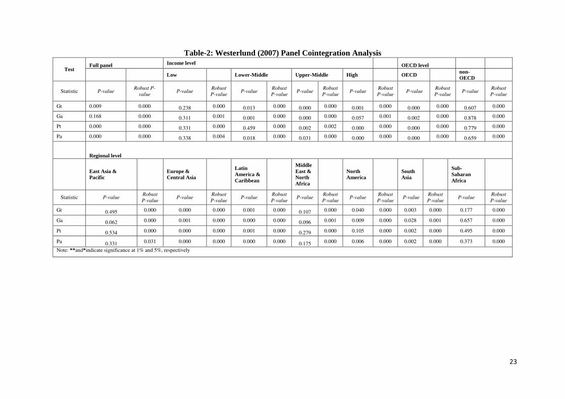
After confirming that the variables are integrated at I(1), we proceed to apply thepanel
cointegration approach developed by Westerlund (2007). The results are reported in Table-2.
We note that the empirical findings of the panel and group statistics lead to rejection of the
null hypothesis of no cointegration in the full panelor at the income, OECD or regional
levels. This result implies the presence of cointegration between the variables over the period
from 1960 to 2014. We may conclude that the long-run relationship between economic
growth, electricity consumption, oil prices, gross fixed capital formation and labor is
supported. For a robust check, we further apply (Pedroni, 1999, 2000, 2001, 2004) a panel
cointegration test, and the results are reported in Table-A2. The panel cointegration test
results confirm the findings of the Westerlund (2007) cointegration test.
For long-run dynamic linkages between the variables, we have applied FMOLS. The results
are shown in Table-3. The empirical results indicate that electricity consumption has a
positive and significant impact on economic growth in the case of the full panel as well as for
lower-middle income, upper-middle income, OECD, East Asia & Pacific, Middle East &
North Africa, South Asia and Sub-Saharan Africa regions. This finding is consistent with

22
those of Streimikiene and Kasperowicz (2016), Tang et al. (2016), and Rafindadi and Ozturk
(2016). Electricity consumption positively (negatively) but non-significantly affects
economic growth in the cases of low-income countries, non-OECD countries, Europe &
Central Asia and Latin America & the Caribbean (high-income countries and North
America). These results show that oil is a more noteworthy energy component than electricity
in these regions.
23
Table-2: Westerlund (2007) Panel Cointegration Analysis
Test Full panel Income level OECD level
Low Lower-Middle Upper-Middle High OECD non-OECD
Statistic P-value Robust P-
value P-value
Robust
P-value P-value
Robust
P-value P-value
Robust
P-value P-value
Robust
P-value P-value
Robust
P-value P-value
Robust
P-value
Gt 0.009 0.000 0.238 0.000 0.013 0.000 0.000 0.000 0.001 0.000 0.000 0.000 0.607 0.000
Ga 0.168 0.000 0.311 0.001 0.001 0.000 0.000 0.000 0.057 0.001 0.002 0.000 0.878 0.000
Pt 0.000 0.000 0.331 0.000 0.459 0.000 0.002 0.002 0.000 0.000 0.000 0.000 0.779 0.000
Pa 0.000 0.000 0.338 0.004 0.018 0.000 0.031 0.000 0.000 0.000 0.000 0.000 0.659 0.000
Regional level
East Asia & Pacific Europe &
Central Asia Latin America & Caribbean
Middle East & North Africa
North America South
Asia Sub-Saharan Africa
Statistic P-value Robust
P-value P-value
Robust
P-value P-value
Robust
P-value P-value
Robust
P-value P-value
Robust
P-value P-value
Robust
P-value P-value
Robust
P-value
Gt 0.495 0.000 0.000 0.000 0.001 0.000 0.107 0.000 0.040 0.000 0.003 0.000 0.177 0.000
Ga 0.062 0.000 0.001 0.000 0.000 0.000 0.096 0.001 0.009 0.000 0.028 0.001 0.657 0.000
Pt 0.534 0.000 0.000 0.000 0.001 0.000 0.279 0.000 0.105 0.000 0.002 0.000 0.495 0.000
Pa 0.331 0.031 0.000 0.000 0.000 0.000 0.175 0.000 0.006 0.000 0.002 0.000 0.373 0.000
Note: **and*indicate significance at 1% and 5%, respectively

24
Table-3: Fully Modified OLS Regression Analysis Group tEln tOln tKln tLln
Full Panel 0.157** 0.241** 0.482** 2.840** Income Level
Low 0.914 1.223** 0.492*** 1.526** Lower-Middle 2.433** 1.541** 0.161*** 0.691** Upper-Middle 0.359** 1.882 1.141*** 0.832 High -0.194 1.704** 0.138*** 0.057** OECD
OECD 0.159** 0.135** 0.448*** 2.672** Non-OECD 2.435 0.374** 0.649*** 2.113** Region
East Asia & Pacific 1.065** 0.997** 0.276*** 2.317** Europe & Central Asia 1.143 1.521 0.493*** 0.549 Latin America & Caribbean 0.612 0.428** 0.835*** 0.581** Middle East & North Africa 1.118** 0.627** 0.924*** 1.217** North America -0.351 0.126** 0.611*** -0.058 South Asia 0.163** 1.507 0.329*** 1.205 Sub-Saharan Africa 0.198** 0.127* 0.849*** 0.242* Note: ** and *indicatesignificance at 1% and 5%, respectively.
Oil price has a positive and significant effect on economic growth. This relationship shows
that the increase in oil price positively affects economic growth in the full panel and in low-
income, lower-middle income, high-income, OECD & non-OECD, East Asia & Pacific, Latin
America & Caribbean, Middle East & North Africa, North America and Sub-Saharan Africa
regions. The positive relationship indicates that energy price-saving and lower oil
pricesmayalso curtail payments for imports (oil). North America is the only region adversely
affected by an increase in oil price. These countries are oil-exporters as well as oil-importers,
and the rapid decline in oil prices has both negative and positive effects on different sectors.
In the case of Canada, real GDP increased by 2.4% in the last quarter of 2014. By contrast,
real incomes contracted due to the value of exports (oil) (Isfeld, 2015). This finding is similar
to that of Alquist and Guénette (2014). In the cases of upper-middle income countries,
Europe & Central Asia and South Asia, oil price has a positive but non-significant impact on
economic growth. This finding of non-significance is in line with Behmiri and Manso (2014),

25
who argue that South Asia, i.e., Pakistan9, India10, Bangladesh, etc. consists of industrial
economies in which oil consumption is continuously increasing regardless of whether oil
price increases or decreases. The non-significance of oil price and the significance of
electricity consumption confirm that electricity has a more prominent role than oil price in
South Asia.
The relationship between gross fixed capital formation and economic growth is positive and
significant in the full panel and in all regions, which implies that capitalization enhances
economic growth significantly. Our empirical evidence is similar to that of Streimikiene and
Kasperowicz (2016), Apergis and Payne (2010) and Satti et al. (2014), who reported that
gross fixed capitalization plays a vital role in stimulating economic activity and hence
stimulates economic growth. The association between labor growth and economic growth is
positive and significant. Labor growth affects economic growth positively and non-
significantly in the full panel and all regions except for upper-income countries, but in North
America, labor growth adversely affects economic growth, albeit non-significantly.
Our empirical evidence indicates the significance of economic growth in all five developing
country categories. Lower-middle income, upper-middle income, East Asia & Pacific, Middle
East & North Africa and South Asia showa significant positive effect of electricity
consumption on economic growth. Oil price is significant for only three of the five
developing country categories. The upper-middle income and South Asia categories
showsignificant results. In sum, the results confirm that developing countries rely heavily on
electricity consumption for economic growthin spite of oil price. Proficient and sound fiscal
9Double-digit percentage increases in oil consumption were recorded by Pakistan between 2012 and 2013 (Rapier, 2014). 10 India became the third-largest oil consumer in 2015 (Meyer and Hume, 2014).

26
policy, monetary policy and industrial infrastructure can mitigate the effect of oil price
shocks on economic growth. Furthermore, we apply panel OLS and dynamic OLS for a
robust check, and the results are reported in Table-A3. The empirical evidence corroborates
the impact of electricity consumption, oil price, capital and labor on economic growth, which
is in line with the FMOLS empirical results. This indicates that long-run empirical results are
reliable and robust.
Table-1: Pool Mean Group Analysis
Dependent Variable
Source of causation (independent variable)
Short-run Long-run
tYln∆ tEln∆ tOln∆ tKln∆ tLln∆ 1−tECT
Full Panel
tYln∆
0.111** 0.063** 0.391** 0.128** 0.0015**
tEln∆ 1.242**
11.214** 0.953 2.528 0.0063**
tOln∆ 31.157** 2.059
0.153 41.250** -0.0040*
tKln∆ 125.548 5.493* 5.846**
2.753** -0.0010
tLln∆ 8.186 24.435** 5.753** 6.197**
0.0011**
Low-Income Panel
tYln∆
4.872 1.559* 0.194 0.772 -0.0107
tEln∆ 0.547
1.183 6.717 0.326 -0.0021**
tOln∆ 8.359 0.141
0.943 1.971** -0.0170
tKln∆ 6.105 4.008 0.513
1.209 0.0011
tLln∆ 2.973 2.466 3.157 0.013
-0.0529*
Low-Middle-Income Panel
tYln∆ 2.593** 1.854** 9.451* 8.937* 0.0081
tEln∆ 5.673 1.775 11.823 7.031 0.0004
tOln∆ 18.209** 3.82 7.106 98.435** 0.0031**
tKln∆ 10.815** 8.006** 9.651** 35.618** -0.0683
tLln∆ 2.607 5.111 11.345** 5.715 0.0018**
Upper-Middle-Income Panel
tYln∆ 25.822* 2.485 12.765** 43.541** -0.0064**
tEln∆ 25.654** 6.908 22.582 12.079 -0.0234*
tOln∆ 3.174** 8.907** 0.135 60.953** -0.0006**
tKln∆ 23.765** 45.079** 4.124* 5.171** 0.0979**
tLln∆ 7.411 2.147 3.159 8.534** -0.0554
High-Income Panel

27
tYln∆ 6.438** 9.022 4.212 16.108** -0.0751**
tEln∆ 52.97** 15.4* 78.505** 0.316 -0.0834**
tOln∆ 11.66* 2.407 8.192 32.0541** -0.0733*
tKln∆ 126.309 3.868 5.627 5.196** 0.0518*
tLln∆ 9.988 14.583** 9.642 6.152 0.0960
OECD
tYln∆ 9.915** 5.892 4.331 2.554** 0.0515*
tEln∆ 1.924** 25.109** 56.491** 6.477 -0.0301**
tOln∆ 75.35 9.774 9.182 8.815 -0.0845*
tKln∆ 65.431 5.706 7.204 5.613 0.0129
tLln∆ 9.007 95.806** 3.114 5.841 0.0015**
Non-OECD
tYln∆ 30.019** 9.082** 5.960 81.102* 0.0056
tEln∆ 5.609 56.806** 8.312 8.081 0.0110
tOln∆ 7.426** 8.185 9.444 99.107** 0.0451*
tKln∆ 14.901** 7.155 17.011** 73.215* 0.0009**
tLln∆ 11.152 0.106 5.131 4.016 0.0061
East Asia & Pacific
tYln∆ 17.151** 1.864** 5.091 2.87** 0.0010**
tEln∆ 53.609** 1.076 5.808** 4.631 -0.0013**
tOln∆ 1.441 3.127 23.514 30.011** -0.0068*
tKln∆ 90.307* 6.936* 6.553 3.792 0.0718
tLln∆ 6.102 109.601* 5.321 2.047 -0.0089
Europe & Central Asia
tYln∆ 1.55* 11.045 32.306** 17.806 0.0020*
tEln∆ 6.609 97.564** 3.104 15.661 -0.0026**
tOln∆ 78.908** 6.342 8.791 52.906* 0.0048
tKln∆ 8.564** 89.013** 1.07 9.155* 0.0917*
tLln∆ 0.896 2.3067** 23.011** 7.155 -0.0806
Latin America & Caribbean
tYln∆ 2.097** 7.869** 15.506 42.807* -0.0501
tEln∆ 4.927* 9.172 13.908 75.432** -0.0001
tOln∆ 13.901** 3.412 54.021 68.195 -0.0047**
tKln∆ 16.071** 8.262 24.456 4.001 0.0098*
tLln∆ 4.051 7.095 34.774 11.092 0.0900*
Middle East& North Africa
tYln∆ 34.698** 1.556 16.201** 5.814* 0.0805
tEln∆ 6.432 6.098 5.816 3.607 0.0017**
tOln∆ 7.098 5.891 9.418 78.809** 0.0091**
tKln∆ 45.78** 6.085** 85.491* 45.293* 0.0035**

28
tLln∆ 2.051 7.119 14.23 3.163 0.0020
North America
tYln∆ 8.123 7.332** 2.613** 7.852 0.0090*
tEln∆ 7.884 8.793 7.133* 6.778 0.0031
tOln∆ 56.078 8.945 7.193 1.091 0.007
tKln∆ 65.901 11.456 9.056 6.093 -0.0057*
tLln∆ 0.186 5.809 0.006 3.654 0.0560
South Asia
tYln∆ 77.012** 3.198* 8.932 15.512** -0.0045
tEln∆ 13.209 4.097 24.521** 3.314 -0.0130**
tOln∆ 57.305** 8.272 2.309 27.501* 0.0860*
tKln∆ 1.384 3.621 3.304 16.907* 0.0011
tLln∆ 6.907 9.174 4.201 7.002 0.0984
Sub-Saharan Africa
tYln∆ 1.089 2.647 6.097** 10.708** 0.0911
tEln∆ 11.078 6.789 4.132 3.776 0.0981
tOln∆ 84.476** 9.057** 5.004 22.986** -0.0866*
tKln∆ 38.907** 8.103** 5.634 8.042 0.0540
tLln∆ 6.092 8.645 8.883 21.907 0.0046*
Note:** and *indicate significance at 1% and 5%, respectively.
The short-run and long-run causality results obtained by the Pool Mean Group (PMG) test are
reported in Table-411. In the long run, we note that the feedback effect between electricity
consumption and economic growth is valid for the full paneland for the upper-middle income,
high income, OECD, East Asia & Pacific and Europe & Central Asia categories. This
empirical evidence is similar to that of Ho and Siu (2007) and Yuan et al. (2008). The
bidirectional relationship specifies that high economic growth stimulates industrial
development and household living standards, which leads to an increase in electricity
consumption. The unidirectional causality from economic growth to electricity consumption
is confirmed inthe low-middle income, Middle East & North Africa and South Asia
11The long-run dynamics are illustrated by the error correction term (ECT) in Table5. The coefficient of the error correction term is significantly negative in the low-income, upper-middle-income, high-income, OECD, East Asia & Pacific, Europe & Central Asia and South Asia categories.

29
categories. Thisempirical evidence is consistent with Costantini and Martini (2010), Shahbaz
and Feridun (2012), and Damette and Seghir (2013). Electricity consumption as the Granger
cause of economic growth is noted in North America. Along similar lines, Masih and Masih
(1996), Wolde-Rufael (2005) and Alam et al. (2015) also reported that economic growth is a
cause of electricity consumption. A neutral effect is also noted in the cases of the low-middle
income panel, non-OECD, Latin America & Caribbean and Sub-Saharan Africa categories.
The bidirectional causality between labor growth and energy consumption is noted for thefull
paneland for the upper-middle income, high-income, OECD, East Asia & Pacific, Middle
East & North Africa and South Asia categories. Labor growth is the Granger cause of energy
consumption in the low-middle income paneland in the Non-OECD, Latin America &
Caribbean, North America and Sub-Saharan Africa categories. Capitalization causes
electricity consumption, and thus, electricity consumption causes economic growth in the
upper-middle income, high-income, Europe & Central Asia and the Middle East & North
Africa categories. Electricity consumption is a cause of capitalization in the full panel as well
as in the low-income, East Asia & Pacific, Europe & Central Asia and South Asia categories.
In the case of the non-OECD, Latin America & Caribbean, and North America categories, we
find that electricity consumption causes capitalization.
In the short run, a feedback effect exists between oil price, electricity consumption and
economic growth in the full panel and in low-middle income, non-OECD, Latin America &
Caribbean and South Asian countries. The unidirectional causality is found from oil price to
economic growth in the low-income, East Asia &Pacific and North America categories, while
economic growth influences oil price in upper-middle income, high income, OECD,
European & Central Asian and Sub-Saharan countries. A neutral effect between oil price and
economic growth is also noted in the Middle East & North Africa. In 2014, Colombia,

30
Venezuela and Ecuador experienced a decline in economic growth due to the fall in oil price.
Meanwhile, Mexico, Brazil, and Argentina experienced moderate economic growth. The
International Monetary Fund (IMF) estimated that Latin America reacts in a mostly neutral
manner, with no net gain from rising or declining oil price. Capital formation and labor force
show a bidirectional relationship with economic growth in the full sample, whereas the
subgroup level depicts different findings.
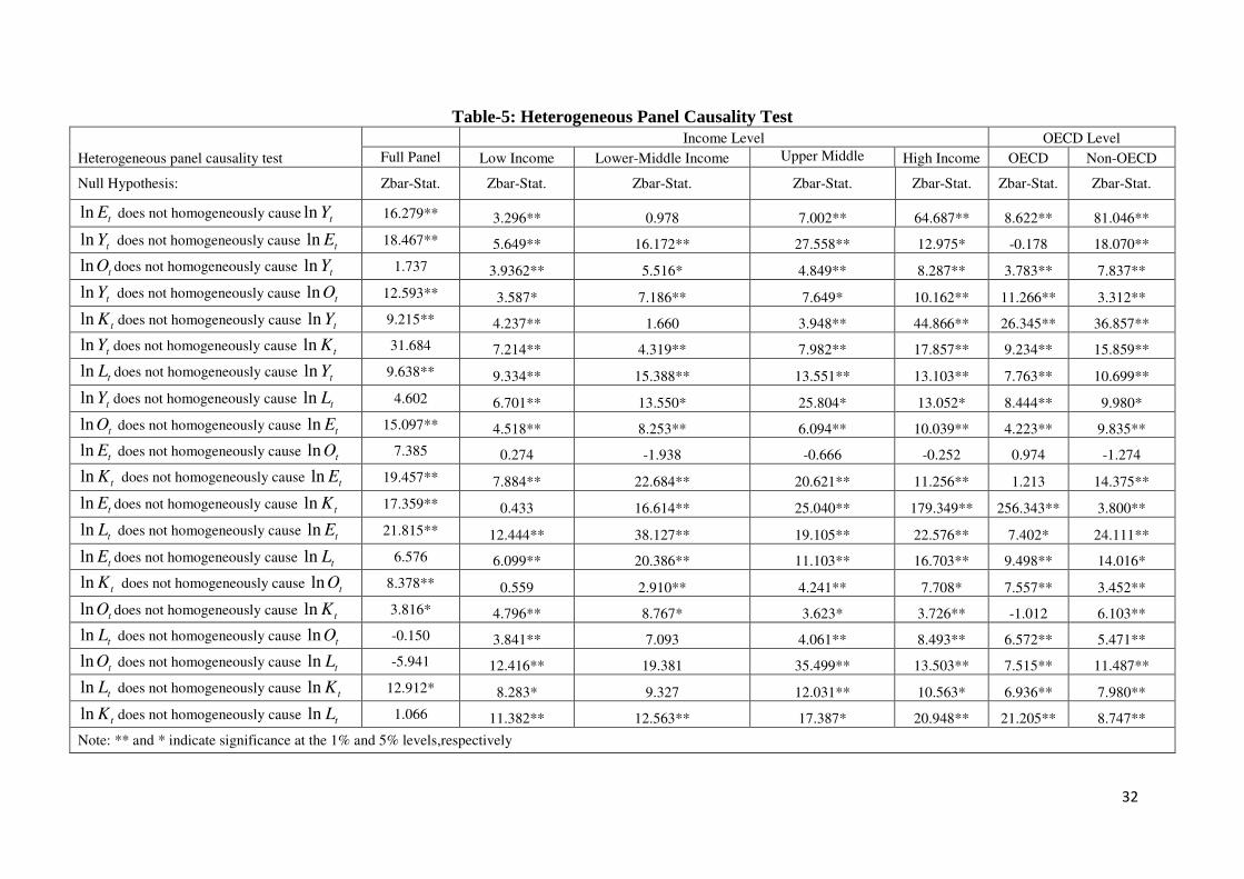
To examine the robustness of the PMG Granger causality test, we have applied the
heterogeneous panel causality test. The results are reported in Table-5. We find that in the
full sample panel, electricity consumption and economic growth have a confirmed
bidirectional causality relationship. However, a unidirectional causal relationship exists from
economic growth to oil price. These results also confirm the significant role of electricity
consumption over oil price for the economy. A feedback effect exists between electricity
consumption and economic growth for the low-income, upper-middle-income, high-income,
non-OECD, East Asia & Pacific, Latin America & Caribbean, Middle East & North Africa,
South Asia and Sub-Saharan Africa categories. This feedback effect indicates that a reduction
in electricity supply will retard economic growth, and thus, a decline in economic growth will
reduce electricity demand. The empirical evidence supports the implementation of energy-
exploring policies to maintain economic development for the long run. The empirical
evidence for the bidirectional causal association between electricity consumption and
economic growth is similar to that ofHo and Siu (2007), Behmiri and Manso (2013), and Al-
mulali and Sab (2012). Economic growth is the Granger cause of electricity consumption in
the case of OECD, while the case of Europe & Central Asia reveals the importance of
consistent electricity supply for long-run economic growth. The unidirectional causality from
electricity consumption to economic growth is consistent with Narayan and Singh (2007),
31
Damette and Seghir (2013), Streimikiene and Kasperowicz (2016) and Tang et al. (2016).
Economic growth is the Granger cause ofelectricity consumption in the lower-middle-income
and Europe & Central Asia categories. The unidirectional causality from economic growth to
electricity consumption is similar to the results of Costantini and Martini (2010).
32
Table-5: Heterogeneous Panel Causality Test
Heterogeneous panel causality test
Income Level OECD Level
Full Panel Low Income Lower-Middle Income Upper Middle Income
High Income OECD Non-OECD
Null Hypothesis: Zbar-Stat. Zbar-Stat. Zbar-Stat. Zbar-Stat. Zbar-Stat. Zbar-Stat. Zbar-Stat.
tEln does not homogeneously cause tYln 16.279** 3.296** 0.978 7.002** 64.687** 8.622** 81.046**
tYln does not homogeneously cause tEln 18.467** 5.649** 16.172** 27.558** 12.975* -0.178 18.070**
tOln does not homogeneously cause tYln 1.737 3.9362** 5.516* 4.849** 8.287** 3.783** 7.837**
tYln does not homogeneously cause tOln 12.593** 3.587* 7.186** 7.649* 10.162** 11.266** 3.312**
tKln does not homogeneously cause tYln 9.215** 4.237** 1.660 3.948** 44.866** 26.345** 36.857**
tYln does not homogeneously cause tKln 31.684 7.214** 4.319** 7.982** 17.857** 9.234** 15.859**
tLln does not homogeneously cause tYln 9.638** 9.334** 15.388** 13.551** 13.103** 7.763** 10.699**
tYln does not homogeneously cause tLln 4.602 6.701** 13.550* 25.804* 13.052* 8.444** 9.980*
tOln does not homogeneously cause tEln 15.097** 4.518** 8.253** 6.094** 10.039** 4.223** 9.835**
tEln does not homogeneously cause tOln 7.385 0.274 -1.938 -0.666 -0.252 0.974 -1.274
tKln does not homogeneously cause tEln 19.457** 7.884** 22.684** 20.621** 11.256** 1.213 14.375**
tEln does not homogeneously cause tKln 17.359** 0.433 16.614** 25.040** 179.349** 256.343** 3.800**
tLln does not homogeneously cause tEln 21.815** 12.444** 38.127** 19.105** 22.576** 7.402* 24.111**
tEln does not homogeneously cause tLln 6.576 6.099** 20.386** 11.103** 16.703** 9.498** 14.016*
tKln does not homogeneously cause tOln 8.378** 0.559 2.910** 4.241** 7.708* 7.557** 3.452**
tOln does not homogeneously cause tKln 3.816* 4.796** 8.767* 3.623* 3.726** -1.012 6.103**
tLln does not homogeneously cause tOln -0.150 3.841** 7.093 4.061** 8.493** 6.572** 5.471**
tOln does not homogeneously cause tLln -5.941 12.416** 19.381 35.499** 13.503** 7.515** 11.487**
tLln does not homogeneously cause tKln 12.912* 8.283* 9.327 12.031** 10.563* 6.936** 7.980**
tKln does not homogeneously cause tLln 1.066 11.382** 12.563** 17.387* 20.948** 21.205** 8.747**
Note: ** and * indicate significance at the 1% and 5% levels,respectively

33
Table 5: Heterogeneous Panel Causality Test (continued)
Null Hypothesis:
Regional Level
East Asia & Pacific
Europe & Central Asia
Latin America & Caribbean
Middle East& North Africa
North America
South Asia
Sub-Saharan Africa
Zbar-Stat. Zbar-Stat. Zbar-Stat. Zbar-Stat. Zbar-Stat. Zbar-Stat. Zbar-Stat.
tEln does not homogeneously cause tYln 2.492** 5.548** 84.012** 4.195** 0.856 2.250** 2.627**
tYln does not homogeneously cause tEln 12.577** 1.904 7.466** 17.113** -0.801 2.063** 33.597**
tOln does not homogeneously cause tYln 3.528** 1.345 9.777** 5.501** 9.489** 2.861** 2.842**
tYln does not homogeneously cause tOln 6.181* 8.283** 4.077* 2.374** -0.518 3.435** 10.808*
tKln does not homogeneously cause tYln -0.340 26.383** 33.145** 7.404** -0.274 3.516** 2.711**
tYln does not homogeneously cause tKln 11.895* 8.460** 6.960** 6.132** -0.050 -0.607 12.199**
tLln does not homogeneously cause tYln 15.300** 8.523** 15.573* 6.978** 2.761** 2.848** 10.816**
tYln does not homogeneously cause tLln 17.431* 9.955** 14.965** 11.373** 1.892 0.839 14.913**
tOln does not homogeneously cause tEln 9.882** 3.726** 6.903** 3.005* 0.910 2.524 9.116**
tEln does not homogeneously cause tOln -1.247 0.437 -2.043 0.351 -0.651 -1.346 0.295
tKln does not homogeneously cause tEln 28.988** 1.346 5.643** 8.806** 1.536 7.470** 24.094
tEln does not homogeneously cause tKln 110.233** 7.691* 11.259** 14.146 520.206** 4.661** 0.283
tLln does not homogeneously cause tEln 49.978** 9.944** 13.644** 3.196* 0.440 5.188** 28.113**
tEln does not homogeneously cause tLln 10.460** 20.070** 6.412** 17.670** 1.252 6.222** 7.880**
tKln does not homogeneously cause tOln 0.929 6.836** 4.148** 2.976** -0.988 0.765 4.028**
tOln does not homogeneously cause tKln 2.768** -0.197 6.580** 5.785** 0.619 -0.061 8.510**
tLln does not homogeneously cause tOln 7.805 3.175** 5.720** 3.007* 4.239** 2.384** 5.804*
tOln does not homogeneously cause tLln 23.436** 3.877* 38.501** 13.407** 1.608 2.649** 12.566**
tLln does not homogeneously cause tKln 12.751** 7.045** 8.847** 5.669** -0.209 3.614** 10.409*
tKln does not homogeneously cause tLln 12.809* 12.945** 13.99** 9.539** 22.971** -0.271 16.478**

34
Shahbaz and Feridun (2012), and Ahmed and Azam (2016). A neutral effect exists between
electricity consumption and economic growth for North America, which suggests that the
implementation of energy conservation policies will not retard economic growth. This lack of
acausal relationship between electricity consumption and economic growth is consistent with
Chontanawat et al. (2008), Zilio and Recalde (2011), Karanfil and Li (2015), and Ahmed and
Azam (2016).
The relationship between oil prices and economic growth is bidirectional for the low-income,
lower-middle-income, upper-middle-income, high-income, OECD, non-OECD, East Asia &
Pacific, Latin America & Caribbean, Middle East & North Africa, South Asia and Sub-Saharan
Africa panels. The unidirectional causality is found from oil price to economic growth in the case
of North America. Similar results are reported by Elmezouar et al. (2014), who argued that most
of these economies are in a transition phase and need oil to boost their economic growth. In such
circumstances, an increase in oil price has no adverse effect on oil-importing and oil-exporting
countries (Rasmussen and Roitman, 2011). Economic growth is the Granger cause of oil price
for the full panel and for Europe & Central Asia. This result implies that economic growth of a
country can be attained by a gradual boost in the industrial sector, which requires energy (oil).
This higher demand for oil causes the oil priceto increase (Ali, 2016). The causality between
gross fixed capitalization and economic growth is bidirectional for the low-income, upper-
middle-income, high-income, OECD, Non-OECD, East Asia & Pacific, Europe & Central Asia,
Latin America & Caribbean, Middle East & North Africa and Sub-Saharan Africa categories.
Capitalization is the Granger cause of economic growth in thecases of the full panel and South
Asia. Economic growth is the Granger cause of capitalization in the lower-middle income and

35
East Asia & Pacific categories, while a neutral effect exists between gross fixed capitalization
and economic growth in North America. A bidirectional causal relationship exists between labor
growth and economic growth in the low-income, upper-middle-income, high income, OECD,
non-OECD, East Asia & Pacific, Europe & Central Asia, Latin America & Caribbean, Middle
East & North Africa and Sub-Saharan Africa categories. In the case of the full panel, North
America and South Asia, labor growth is the Granger cause of economic growth.
5. Summary and Conclusion
This study uses the data from 157 countries over the period from 1960 to 2014 to examine the
empirical relationship between electricity consumption and economic growth by incorporating
oil price as an additional factor of production. The data are categorized into income, OECD and
regional levels. The cointegration approach developed by Westerlund (2007) is applied to
examine cointegration between the variables. The pool mean group test is used to study the
short-run and long-run relationships between variables. The robustness of the empirical analysis
is also tested by applying alternative unit root, cointegration and causality approaches.
We find evidence of cointegration between the variables. Moreover, electricity consumption
stimulates economic growth in the full panel and the lower-middle-income, upper-middle
income, OECD, East Asia & Pacific, Middle East & North Africa, South Asia and Sub-Saharan
Africa regions. A positive association between oil price and economic growth is confirmed for
the full panelas well as for the low-income, lower-middle-income, high-income, OECD, Non-
OECD, East Asia & Pacific, Latin America & Caribbean, Middle East & North Africa, North
America and Sub-Saharan Africa panels. Capitalization and labor growth promote economic

36
growth in the full panel and in all regions. Electricity consumption causes economic growth, and
as a result, economic growth causes electricity consumption in the full panel as well as the
upper-middle income, high income, OECD, East Asia & Pacific and Europe & Central Asia
categories. The energy conservation hypothesis is valid for the lower-middle-income, Middle
East & North Africa and South Asia groups. The growth hypothesis is noted for North America.
There is no causality between economic growth and electricity consumption in the low-middle-
income panelor in the non-OECD, Latin America & Caribbean and Sub-Saharan Africa
categories.
These empirical findings have significant implications for countries across the regions in
planning for energy conversion policies that help to trigger economic growth. It is suggested that
countries where the growth hypothesis is confirmed find the best alternatives to electricity
generation to enhance economic growth. The countries in which the conservation hypothesis is
confirmed do not depend on electricity for economic growth. These countries should concentrate
on means of economic growth other than electricity policies. For the countries confirming the
feedback hypothesis, the implication is that economic growth and electricity consumption are
mutually dependent; accordingly, policy makers should concentrate onelectricity generation
policies and economic growth policies that stimulate each other. Countries in which the
neutrality hypothesis is confirmed should not pursue economic growth but instead make
electricity conservation policies.
In oil-importing countries, it has been found to be practically impossible to eliminate the
detrimental role of energy prices for economic growth because the elimination of such energy

37
prices, i.e., oil price, would restrain economic growth. Other than the elimination of energy
prices, programs should be implemented to increase the yield, which leads to significantly
increased benefits. Any increase in energy prices results in an increased cost of living for the
citizens. However, addressing this problem is not a major issue because the governments of the
countries can implement specific measures to address the problem. Additionally, it is the
obligation of any government to lower the cost of living for its citizens, particularly the low-
income group, by controlling energy prices.
References
Abdoli, G., Dastan, S., 2015. Electricity consumption and economic growth in OPEC countries:
a cointegrated panel analysis. OPEC Energy Review, 39(1), 1-16.
Abosedra, S., Dah, A., Ghosh, S., 2009. Electricity consumption and economic growth, the case
of Lebanon. Applied Energy, 86(4), 429–432.
Ahmed , M., Azam, M., 2016. Causal nexus between energy consumption and economic.
Renewable and Sustainable Energy Reviews, 60, 653–678.
Alam, M. J., Begum, I. A., Buysse, J., Huylenbroeck, G. V., 2015. Energy consumption, carbon
emissions and economic growth nexus in Bangladesh: Cointegration and dynamic causality
analysis. Energy Policy, 45, 217–225.
Ali, S., 2016. The impact of oil price on economic growth: Test of Granger causality, the case of
OECD countries. International Journal of Social Science and Economic Research, 1(9),
1333-1349.
Allcott, H., Collard-Wexler, A., O'Connell, S. D., 2014. How Do Electricity Shortages Affect
Industry? American Economic Review, 106(3), 587-624.
38
Al-mulali, U., Sab, C. N., 2012. The impact of energy consumption and CO2 emission on the
economic growth and financial development in the Sub Saharan African countries. Energy,
39(1), 180–186.
Alquist, R., Guénette, J.-D. (2014). A blessing in disguise: The implications of high global oil
prices for the North American market. Energy Policy, 64, 49–57.
Apergis, N., Payne, J. E., 2010. A panel study of nuclear energy consumption and economic
growth. Energy Economics, 32, 545-549.
Apergis, N., Payne, J., 2011. A dynamic panel study of economic development and the
electricity consumption-growth nexus. Energy Economics, 33(5), 770–781.
Arellano, M., Bond, S., 1991. Some tests of specification for panel data: Monte Carlo evidence
and an application to employment equations. Journal Review of Economic Studies, 58, 277-
297.
Arellano, M., Bover, O., 1995. Another look at the instrumental variable estimation of error-
components models. Journal of Econometrics, 68(1), 29–51.
Asafu-Adjaye, J., 2000. The relationship between energy consumption, energy prices and
economic growth: time series evidence from Asian developing countries. Energy Economics,
22(6), 615–625.
Bartleet, M., Gounder, R., 2010. Energy consumption and economic growth in New Zealand:
Results of trivariate and multivariate models. Energy Policy, 38(7), 3508–3517.
Behmiri, N. B., Manso, J. P., 2013. How crude oil consumption impacts on economic growth of
Sub-Saharan Africa? Energy, 54, 74–83.
Blundell, R., Bond, S., 1998. Initial conditions and moment restrictions in dynamic panel data
models. Journal of Econometrics, 87(1), 115–143.
39
Breusch, T., Pagan, A., 1980. The LM test and its application to model specification in
econometrics. Review of Economic Studies, 47(1), 239-253.
Chen, S.-T., Kuo, H.-I., Chen, C.-C., 2007. The relationship between GDP and electricity
consumption in 10 Asian countries. Energy Policy, 35(4), 2611–2621.
Cheng, B. S., Lai, T. W., 1997. An investigation of co-integration and causality between energy
consumption and economic activity in Taiwan. Energy Economics, 19(4), 435–444.
Chontanawat, J., Hunt, L., Pierse, R., 2008. Does energy consumption cause economic growth?
Evidence from a systematic study of over 100 countries. Journal of Policy Modeling, 30(2),
209–220.
Ciarreta, A., Zarraga, A., 2008. Economic growth and electricity consumption in 12 European
Countries: a causality analysis using panel data. Department of Applied Economics III
(Econometrics and Statistics), University of the Basque Country.
Costantini, V., Martini, C., 2010. The causality between energy consumption and economic
growth: A multi-sectoral analysis using non-stationary cointegrated panel data. Energy
Economics, 32 (3), 591–603.
Damette, O., Seghir, M., 2013. Energy as a driver of growth in oil exporting countries? Energy
Economics, 37, 193-199.
Das, A., Chowdhury, M., Khan, S., 2012. The dynamics of electricity consumption and growth
nexus: Empirical evidence from three developing regions. Journal of Applied Economic
Research, 6, 445-466.
Doroodian, K., Boyd, R., 2003. The linkage between oil price shocks and economic growth with
inflation in the presence of technological advances: a CGE model. Energy Policy, 31(10),
989–1006.

40
Dumitrescu, E.-I., Hurlin, C., 2012. Testing for Granger non-causality in heterogeneous panels.
Economic Modelling, 29 (4), 1450-1460.
Erdal, G., Erdal, H., Esengün, K., 2008. The causality between energy consumption and
economic growth in Turkey. Energy Policy, 36 (10), 3838–3842.
Farzanegan, M. R., Markwardt, G. 2009. The effects of oil price shocks on the Iranian economy.
Energy Economics, 31, 134–151.
Ferguson, R., Wilkinson, W., Hill, R., 2000. Electricity use and economic development. Energy
Policy, 28, 923-934.
Ftiti, Z., Guesmi, K., Teulion, F., Chouachi, S., 2016. Relationship between crude oil prices and
economic growth in selected OPEC countries. The Journal of Applied Business Research, 32,
11-22.
Ghalayini, L., 2011. The interaction between oil price and economic growth. Middle Eastern
Finance and Economics, 13, 127-141.
Ghali, K. H., El-Sakka, M., 2004. Energy use and output growth in Canada: a multivariate
cointegration analysis. Energy Economics, 26(2), 225–238.
Gisser, M., Goodwin, T. H., 1986. Crude oil and the macroeconomy: Tests of some popular
notions. Journal of Money, Credit and Banking, 18(1), 95-103.
Granger, C. W., 1969. Investigating causal relations by econometric models and cross-spectral
methods. The Econometric Society, 37(3), 424-438.
Hamilton, J. D., (1985). Historical causes of postwar oil shocks and recessions. Energy Journal,
6(1), 97-116.
Hamilton, J. D., 1983. Oil and the macroeconomy since World War II. Journal of Political
Economy, 91 (2), 228-248.
41
He, Y., Fullerton, T. M., Walke, A. G., 2017. Electricity consumption and metropolitan
economic performance in Guangzhou: 1950-2013. Energy Economics, 63, 154-160.
Ho, C., Siu, K., 2007. A dynamic equilibrium of electricity consumption and GDP in Hong
Kong: an empirical investigation. Energy Policy, 35, 2507-2513.
Hsiao, C., Pesaran, M., Tahmiscioglu, A., 1999. Analysis of panels and limited dependent
variables: A volume in honour of G. S. Maddala. In Bayes estimation of short-run
coefficients in dynamic panel data models. (pp. 268–296). Cambridge: Cambridge University
Press.
Im, K., Pesaran, H., Shin, Y., 1997. Testing for Unit Roots in Heterogeneous Panels. University
of Cambridge, Mimeo
Isfeld, G., 2015. Low oil to have 'both positive and negative effects' on Canadian economy,
Ottawa Told. Financial Post.
Iyke, B., 2015. Electricity consumption and economic growth in Nigeria: A revisit of the energy-
growth debate. Energy Economics, 51, 166-176.
Jayaraman, T.K., Choong, C.-K., 2009. Growth and oil price: A study of causal relationship in
small Pacific Island countries. Energy Policy, 37(6), 2182-2189.
Jbir, R., Zouari-Ghorbel, S., 2009. Recent oil price shock and Tunisian economy. Energy Policy.
37(3), 1041–1051.
Jimnez-Rodrguez, R., Snchez, M., 2005. Oil price shocks and real GDP growth: empirical
evidence for some OECD countries. Applied Economics, 37, 201-228.
Johansen, S., Juselius, K., 1990.Maximum likelihood estimation and inference on cointegration
with applications to demand for money. Oxford Bulletin of Economics and Statistics, 52,
169-210.
42
Kahane, A., Squitieri, R., 1987. Electricity Use in Manufacturing. Annual Review of Energy, 12,
223-251.
Kao, C., Chiang, M.-H., 2000.On the estimation and inference of a cointegrated regression in
panel data. Nonstationary Panels, Panel Cointegration and Dynamic Panels, 15, 179–222.
Karanfil, F., Li, Y., 2015. Electricity consumption and economic growth: Exploring panel-
specific differences. Energy Policy, 28, 264–277.
Kasman, A., Duman, Y.S., 2015. CO2 emissions, economic growth, energy consumption, trade
and urbanization in new EU member and candidate countries: a panel data analysis.
Economic Modelling 44, 97-103.
Kayıkçı, F., Bildirici, M., 2015. Economic growth and electricity consumption in GCC and
MENA countries. South African Journal of Economics, 83(2), 303–316.
Khan, M.A., Qayyum, A., Ahmad, E., 2007. Dynamic modelling of energy and growth in South
Asia. Pakistan Development Review 46, 481–498.
Kilian, L., 2008. Exogenous oil supply shocks: How big are they and how much do they matter
for the U.S. economy? Review of Economics and Statistics, 90(2), 216-240.
Kilian, L., Vigfusson, R. 2011. Are the responses of the U.S. economy asymmetric in energy
price increases and decreases? Quantitative Economics, 2(3), 419-453.
Lardic, S., Mignon, V., 2006. The impact of oil prices on GDP in European countries: An
empirical investigation based on asymmetric cointegration. Energy Policy, 34, 3910-3915.
Lee, C.-C., Chang, C.-P., Chen, P.-F., 2008. Energy-income causality in OECD countries
revisited: The key role of capital stock. Energy Economics, 30(5), 2359–2373.
Maeda, A., 2008. On the oil price-GDP relationship. Japanese Economy, 35, 99-127.

43
Mahmoodi, M., Mahmoodi, E., 2011. Renewable energy consumption and economic growth: the
case of 7 Asian developing countries. American Journal of Scientific Research 35, 146–152.
Masih, A. M., Masih, R. 1996. Energy consumption, real income and temporal causality: results
from a multi-country study based on cointegration and error-correction modelling techniques.
Energy Economics, 18, 165–183.
Masih, A.M.M., Masih, R., 1996. Energy consumption, real income and temporal causality:
results from a multi-country study based on cointegration and error-correction modelling
techniques. Energy Economics 18, 165–183.
Mehrara, M. 2007. Energy consumption and economic growth: The case of oil exporting
countries. Energy Policy, 35(5), 2939–2945.
Mehrara, M., 2008. The asymmetric relationship between oil revenues and economic activities:
the case of oil-exporting countries. Energy Policy 36, 1164–1168.
Meyer, G., Hume , N., 2016. Booming petrol demand from US to India buoys oil price.
Retrieved from Financial Times: https://www.ft.com/content/65dc4f9a-1d6f-11e6-b286-
cddde55ca122?ftcamp=published_links/rss/markets_commodities/feed//productandutm_sour
ce=twitterfeedandutm_medium=twitter
Morey, J. F., 1993. Oil Prices and Economic Activity: Is the Relationship Symmetric? The
Energy Journal, 14, 151-161.
Mork, K. A., 1989. Oil and macroeconomy when prices go up and down: An extension of
Hamilton's results. Journal of Political Economy, 97(3), 740-744.
Murray, D., Nan., 1996. A definition of the gross domestic product-electrification inter
relationship. Journal of Energy and Development, 19, 275-283.
44
Murry, D.A., Nan, G.D., 1994. A definition of the gross domestic product-electrification
interrelationship. Journal of Energy and Development 19, 275–283.
Mutascu, M., 2016. A bootstrap panel Granger causality analysis of energy consumption.
Renewable and Sustainable Energy Reviews, 63, 166–171.
Mutascu, M., 2016. A bootstrap panel Granger causality analysis of energy consumption.
Renewable and Sustainable Energy Reviews, 63, 166–171.
Narayan, P. K., Prasad, A., 2008. Electricity consumption–real GDP causality nexus: Evidence
from a bootstrapped causality test for 30 OECD countries. Energy Policy, 36(2), 910–918.
Narayan, P.K., Narayan, S., Popp, S., 2010. Does electricity consumption Granger cause GDP?
New global evidence. Applied Energy, 87, 3294-3298.
Narayana, P. K., Singh, B., 2007. The electricity consumption and GDP nexus for the Fiji
Islands. Energy Economics, 29(6), 1141–1150.
Osman, M., Gachino, G., Hoque, A., 2016. Electricity consumption and economic growth in the
GCC countries: Panel data analysis. Energy Policy, 98, 318–327.
Ozlale, U., Pekkurnaz, D., 2010. Oil prices and current account: A structural analysis for the
Turkish economy. Energy Policy, 38, 4489-4496.
Ozturk, I., 2010. Literature survey on energy–growth nexus. Energy Policy, 38(1), 340–349.
Ozturk, I., Acaravci, A., 2011. Electricity consumption and real GDP causality nexus: Evidence
from ARDL bounds testing approach for 11 MENA countries. Applied Energy, 88, 2885-
2892.
Payne, J., 2010. A survey of the electricity consumption-growth literature.Applied Energy, 87,
723-731.
45
Pedroni, P., 1999. Critical values for cointegration tests in heterogeneous panels with multiple
regressors. Oxford Bulletin of Economics and Statistics, 61(0), 653-670.
Pedroni, P., 2000. Fully modified OLS for heterogeneous cointegrated panels. Advances in
Econometrics, 15, 93-130.
Pedroni, P., 2001. Purchasing power parity tests in cointegrated panels. The Review of
Economics and Statistics, 727-731.
Pedroni, P., 2004. Panel cointegration: Asymptotic and finite sample properties of pooled time
series tests with an application to the purchasing power parity hypothesis. Econometric
Theory, 20, 597-625.
Pesaran, H., 2004. General diagnostic tests for cross section dependence in panels. CESifo
Working, No. 1229.
Pesaran, H., 2007. A simple panel unit root test in the presence of cross section dependence.
Journal of Applied Econometrics, 22(2), 265-312.
Pesaran, H., Shin, Y., Smith, R., 1999. Pooled mean group estimation of dynamic heterogeneous
panels. Journal of the American Statistical Association, 94, 621–634.
Pesaran, M. H., Shin, Y., Smith, R. J., 2001. Bounds testing approaches to the analysis of level
relationships. Journal of Applied Econometrics, 16, 289-326.
Polemis, M.L., Dagoumas, A.S., 2013. The electricity consumption and economic growth nexus:
Evidence from Greece. Energy Policy, 62, 798-808.
Pradhan, R.P., 2010. Energy consumption-growth nexus in SAARC countries: using
cointegration and error-correction model. Modern Applied Science 4, 74–90.

46
Rafindadi, A. A., Ozturk, I., 2016. Effects of financial development, economic growth and trade
on electricity consumption: Evidence from post-Fukushima Japan. Renewable and
Sustainable Energy Reviews, 54, 1073-1084.
Rapier, R., 2014. World sets new oil production and consumption records. Retrieved from
Energy Trends Report: http://www.energytrendsinsider.com/2014/07/10/world-sets-new-oil-
production-and-consumption-records/
Shahbaz, M. and Ali, A. (2016). Measuring Economic Cost of Electricity Shortage: Current
Challenges and Future Prospects in Pakistan. Bulletin of Energy Economics, 4, 211- 223.
Satti, S. L., Hassan, M. S., Mahmood, H., Shahbaz, M., 2014. Coal consumption: An alternate
energy resource to fuel economic growth in Pakistan. Economic Modelling, 36, 282–287.
Shahbaz, M., Feridun, M., 2012. Electricity consumption and economic growth empirical
evidence from Pakistan. Qual Quant, 46, 1583-1599.
Shahbaz, M., Lean, H. H., 2012. Does financial development increase energy consumption? The
role of industrialization and urbanization in Tunisia. Energy Policy, 40, 473-79.
Shahbaz, M., Mallick, H., Mahalik, M.K., Sadorsky, P., 2016. The role of globalization on the
recent evolution of energy demand in India: Implications for sustainable development.
Energy Economics, 55, 52-68.
Shahbaz, M., Zeshan, M., Afza, T., 2012. Is energy consumption effective to spur economic
growth in Pakistan? New evidence from bounds test to level relationships and Granger
causality tests. Economic Modelling 29, 2310–2319.
Shiu, A., Lam, P., 2004. Electricity consumption and economic growth in China. Energy Policy,
32, 47-54.

47
Smiech, S., Papiez, M., 2014. Energy consumption and economic growth in the light of meeting
the targets of energy policy in the EU: the bootstrap panel Granger causality approach.
Energy Policy 71, 118-129.
Solow, R. M., 1956. A contribution to the theory of economic growth. The Quarterly Journal of
Economics, 70(1), 65-94.
Soytas, U., Sari, R., 2003. Energy consumption and GDP: causality relationship in G-7 countries
and emerging markets. Energy Economics, 25(1), 33–37.
Squalli, J., 2007. Electricity consumption and economic growth: bounds and causality analyses.
Energy Economics, 29(6), 1192–1205.
Streimikiene, D., Kasperowicz, R., 2016. Review of economic growth and energy consumption:
A panel cointegration analysis for EU countries. Renewable and Sustainable Energy
Reviews, 59, 1545–1549.
Tang, C. F., Shahbaz, M., 2013. Sectoral analysis of the causal relationship between electricity
consumption and real output in Pakistan. Energy Policy, 60, 885-891.
Tang, C. F., Tan, B. W., Ozturk, I., 2016. Energy consumption and economic growth in Vietnam.
Renewable and Sustainable Energy Reviews, 54, 1506-1514.
Tang, W., Wu, L., Zhnag, Z. X., 2010. Oil price shocks and their short- and long-term effects on
the Chinese economy. Energy Economics, 32, 3–14.
Timilsina, G. R., 2015. Oil prices and the global economy: A general equilibrium analysis.
Energy Economics, 49, 669–675.
Toda, H. Y., Yamamoto, T., 1995. Statistical inference in Vector Autoregressions with possibly
integrated processes. Journal of Econometrics, 66, 225-250.

48
Westerlund, J., 2007. Testing for error correction in panel data. Oxford Bulletin of Economics
and Statistics, 69(6), 709–748.
Wolde-Rufael, Y., 2004. Disaggregated industrial energy consumption and GDP: the case of
Shanghai, 1952–1999. Energy Economics, 26(1), 69–75.
Wolde-Rufael, Y., 2005. Energy demand and economic growth: the African experience. Journal
of Policy Modeling, 27, 891–903.
Wolde-Rufael, Y., 2006. Electricity consumption and economic growth: a time series experience
for 17 African countries. Energy Policy, 34, 1106-1114.
Wolde-Rufael, Y., 2009. Energy consumption and economic growth: the experience of African
countries revisited. Energy Economics 31, 217-224.
Wolde-Rufael, Y., 2014. Electricity consumption and economic growth in transition countries: A
revisit using bootstrap panel Granger causality analysis. Energy Economics, 44, 325-330.
Xundi, D., Liyin, S., Saixing, Z., Jorge, O. J., Xiaoling, Z., 2010. Relationship between energy
consumption and economic development in construction industry. Journal of Engineering.
Design and Technology, 8(3), 257-273.
Yoo, S., 2006.The causal relationship between electricity consumption and economic growth in
the ASEAN countries. Energy Policy, 34, 3573-3582.
Yoo, S., Kwak, S., 2010. Electricity consumption and economic growth in seven south American
countries. Energy Policy, 38, 181-188.
Yu, E.S.H., Hwang, B.K., 1984. The relationship between energy and GNP: further results.
Energy Economics, 6, 186–190.
Yuan, J., Zhao, C., Yu, S., Hu, Z., 2007. Electricity consumption and economic growth in China:
Cointegration and co-feature analysis. Energy Economics, 29(6), 1179–1191.

49
Yuan, J.-H., Kang, J.-G., Zhao, C.-H., Hu, Z.-G., 2008. Energy consumption and economic
growth: Evidence from China at both aggregated and disaggregated levels. Energy
Economics, 30(6), 3077–3094.
Zilio, M., Recalde, M., 2011. GDP and environment pressure: The role of energy in Latin
America and the Caribbean. Energy Policy, 39(12), 7941–7949.
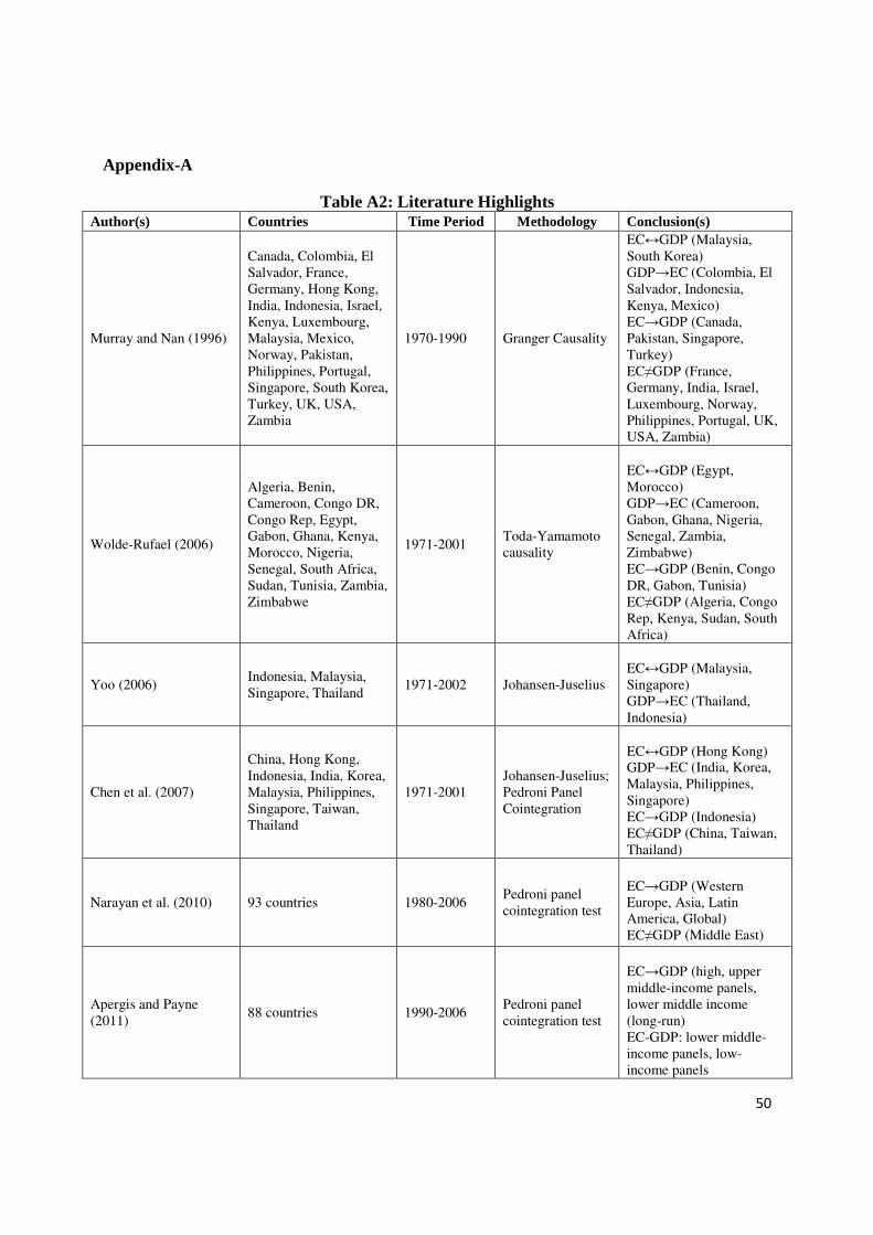
50
Appendix-A
Table A2: Literature Highlights Author(s) Countries Time Period Methodology Conclusion(s)
Murray and Nan (1996)
Canada, Colombia, El Salvador, France, Germany, Hong Kong, India, Indonesia, Israel, Kenya, Luxembourg, Malaysia, Mexico, Norway, Pakistan, Philippines, Portugal, Singapore, South Korea, Turkey, UK, USA, Zambia
1970-1990 Granger Causality
EC↔GDP (Malaysia, South Korea) GDP→EC (Colombia, El Salvador, Indonesia, Kenya, Mexico) EC→GDP (Canada, Pakistan, Singapore, Turkey) EC≠GDP (France, Germany, India, Israel, Luxembourg, Norway, Philippines, Portugal, UK, USA, Zambia)
Wolde-Rufael (2006)
Algeria, Benin, Cameroon, Congo DR, Congo Rep, Egypt, Gabon, Ghana, Kenya, Morocco, Nigeria, Senegal, South Africa, Sudan, Tunisia, Zambia, Zimbabwe
1971-2001 Toda-Yamamoto causality
EC↔GDP (Egypt, Morocco) GDP→EC (Cameroon, Gabon, Ghana, Nigeria, Senegal, Zambia, Zimbabwe) EC→GDP (Benin, Congo DR, Gabon, Tunisia) EC≠GDP (Algeria, Congo Rep, Kenya, Sudan, South Africa)
Yoo (2006) Indonesia, Malaysia, Singapore, Thailand
1971-2002 Johansen-Juselius
EC↔GDP (Malaysia, Singapore) GDP→EC (Thailand, Indonesia)
Chen et al. (2007)
China, Hong Kong, Indonesia, India, Korea, Malaysia, Philippines, Singapore, Taiwan, Thailand
1971-2001 Johansen-Juselius; Pedroni Panel Cointegration
EC↔GDP (Hong Kong) GDP→EC (India, Korea, Malaysia, Philippines, Singapore) EC→GDP (Indonesia) EC≠GDP (China, Taiwan, Thailand)
Narayan et al. (2010) 93 countries 1980-2006 Pedroni panel cointegration test
EC→GDP (Western Europe, Asia, Latin America, Global) EC≠GDP (Middle East)
Apergis and Payne (2011)
88 countries 1990-2006 Pedroni panel cointegration test
EC→GDP (high, upper middle-income panels, lower middle income (long-run) EC-GDP: lower middle-income panels, low-income panels

51
Karanfil and Li (2015) 160 countries 1980-2010 Panel cointegration test
EC and GDP relation varies across panels.
Osman et al. (2016) GCC countries 1975-2012 PMGE, PMG, AMG, MGE and DFE
EC↔ GDP
Note: EC and GDP denote energy consumption and economic growth, respectively. ↔, →and ≠ indicate the feedback effect, unidirectional causality and neutral effect between the variables. PMGE, PMG, AMG, MGE and DFE represent the pooled mean group estimator, pooled mean group, average mean group, mean group estimator and dynamic fixed effect models.
Table A1: IPS Unit Root Test Analysis IPS at level first difference
tYln 5.263 -49.848**
tEln 3.57 -60.903**
tOln 7.817 -50.426**
tKln 3.921 -45.288**
tLln 7.468 -23.218**
Note: ** and * indicate significance at the 1% and 5% levels, respectively

52
Table A2: Pedroni Panel Cointegration
Test Full panel Income level OECD level
Low Lower-Middle Upper-Middle High OECD Non-OECD Panel ν-statistics 8.897 0.272 4.264214 5.476 5.039 -0.184 3.911**
Panel ρ-statistics -9.234** -7.831** -3.922871 -6.065** -4.561** -7.467** -3.000*
Panel PP-statistics -14.353** -12.372** -5.437567 -10.783** -6.937** -13.194** -4.449**
Panel ADF-statistics -8.544** -6.562** -3.940809 -10.796* 0.381** -9.788** 1.033
Group ρ-statistics -2.951** -1.333 0.554735 -2.627** -2.303* -0.144 -3.040**
Group PP-statistics -10.277** -4.348** -2.469** -6.616 -6.775** -3.826 -5.710**
Group ADF-statistics -5.509** -3.535** -1.023679 -3.271 -3.358** -3.163 -1.627
Regional level
East Asia & Pacific
Europe & Central Asia
Latin America & Caribbean
Middle East& North Africa
North America
South Asia
Sub-Saharan Africa
Panel ν-statistics 3.791 3.139 6.260** 1.918 -1.416 1.441 4.336
Panel ρ-statistics -3.546 -2.939 -5.487** -3.909 -2.273* -1.855 -9.391
Panel PP-statistics -4.73 -4.422** -9.881** -6.850** -4.857** -4.212** -14.790**
Panel ADF-statistics -3.548 1.017 -12.091** -2.743** -4.577** -1.529** -6.152**
Group ρ-statistics -0.364 -0.276 -2.294* -2.127* -1.888* -1.380 -0.724
Group PP-statistics -2.156* -3.558** -4.592** -5.322** -4.575** -6.148** -3.928**
Group ADF-statistics -0.089 -1.252 -3.022** -3.021** -3.462** -3.954** -2.408**
Note: **and * indicate significance at 1% and 5%, respectively.

53
Table A3: Panel Dynamic and Ordinary Least Square
Groups Dynamic Ordinary Least Square (DOLS)
Ordinary Least Square (OLS)
tEln tOln tKln tLln tEln tOln tKln tLln
Full Panel 0.354** 0.478** 0.180** 0.077 0.284** 0.158** 0.790** -0.086**
Income Level Low 0.133** 0.035 0.021 1.682** 0.818** -0.237** 0.564** 0.405**
Lower-Middle 0.237** 0.454** -0.047** 0.421** -0.446** 0.458** 0.508** -0.121
Upper-Middle 0.415** 0.325** 0.174** -0.035 0.923** -0.038 0.631** 0.099
High 0.151** 0.315** 0.665** 0.507** 0.069* 0.158** 1.042** 0.062*
OECD
OECD -0.012 0.298** 0.522** 1.582** 0.202** -0.020 1.091** -0.056
Non-OECD 0.347** 0.449** 0.658** 0.073 -0.025 0.531** 0.770** 0.085
Region
East Asia & Pacific
0.218** -0.060 0.075** 2.492** -0.144** 0.214** 0.719** 0.324**
Europe & Central Asia
0.294** 0.557** 0.177** 0.028 0.641** 0.209** 0.737** 0.069
Latin America & Caribbean
0.483** 0.356** 0.492** -0.249 1.160** -0.438** 0.915** -0.040
Middle East & North Africa
0.327** 0.706** 0.024 0.256* 0.083** 0.684** 0.116** 0.397**
North America 0.893* 0.198 0.524** -2.028* 0.159** 0.776** 0.118** -3.354**
South Asia -0.037 -0.008 0.557** -0.121 -1.474 1.025** 0.790** -1.135
Sub-Saharan Africa
0.046 0.207** 0.019* 1.612** 0.702** -0.087 0.566** 0.622**
Note: ** and * indicate significance at 1% and 5%, respectively