Modeling Dependence Structures in the Electricity Price ...

T L E M S

Modeling DependenceStructures in the ElectricityPrice Business by Means of

Copula Techniques

Hui Zheng

D M S

C U T U G

G, S, 2010

M D S EP B M C T

H Z

c© H Z, 2010

D M S

C U T

SE-41296 G, S

P:+46 76 583 8765

ISSN

M T R 2010

P S, 2010

2

Abstract

The electricity market has reconstructed a new type of financial and economic model. With the

rapid growth of the financial derivatives and the security concern of the deregulated electricity

market, the modeling for electricity futures price has become an important topic, especially for

the practitioners. The traditional method is to calculate the linear correlation between two vari-

ables or to measure whether the two derivatives follow the same trend of movement under the

assumption of joint elliptically distribution. However, the above method cannot fully describe all

the dependencies between two random variables, such as lower tail, upper tail and center depen-

dency. Therefore, we introduce the copula analysis method,which includes the description of

these dependencies. The objective of this thesis is to applythe copula technique to analyze the

various relevant future prices in the electricity market, then to compile the real data to investigate

the intrinsic link and relevant structure between them, andfinally to find the best model to simu-

late the real world data. The theory of this thesis is based onthe Archimedean copula and elliptic

copula. Firstly, a most proximate copula model, either single or mixed, is estimated based on the

real data in 2D. Then, based on the same theory, the application in 2D is extended to 3D, and the

3D copula is generated by applying the similar method.

KEYWORDS : Copula, Dependence , Correlation, Electricity

Acknowledgements

I sincerely appreciate Prof. Patrik Albin for his kind supervising and valuable suggestions.

Meanwhile, I am very grateful of Mr. Alain Angeralides for helping me collecting the data.

Contents

Abstract i

Acknowledgements ii

1 Introduction 3

2 Basic Copula Functions 5

2.1 Definition and Properties . . . . . . . . . . . . . . . . . . . . . . . . . .. . . 5

2.2 Frechet Bounds . . . . . . . . . . . . . . . . . . . . . . . . . . . . . . . . . . 7

2.3 The Dependence Structure . . . . . . . . . . . . . . . . . . . . . . . . . .. . . 7

2.4 The Linear Correlation . . . . . . . . . . . . . . . . . . . . . . . . . . . .. . . 10

2.5 The Probability Density Function of Copulas . . . . . . . . . .. . . . . . . . . 12

2.6 Derivation of copulas : Survival Copulas . . . . . . . . . . . . .. . . . . . . . 12

2.7 Non-parameter copula :Empirical Copulas . . . . . . . . . . . .. . . . . . . . 15

2.8 Mixture Copulas . . . . . . . . . . . . . . . . . . . . . . . . . . . . . . . . . .15

3 Copulas Family Examples 16

3.1 Archimedean Copulas . . . . . . . . . . . . . . . . . . . . . . . . . . . . . .. 17

3.2 Bivariate Copulas examples . . . . . . . . . . . . . . . . . . . . . . . .. . . . 17

3.3 Extreme Value Copulas . . . . . . . . . . . . . . . . . . . . . . . . . . . . .. . 24

3.4 FrWchetõHoeffding Family . . . . . . . . . . . . . . . . . . . . . . . . . . . . 26

4 Sampling Random Number for Copulas Models 27

4.1 The Generation Method . . . . . . . . . . . . . . . . . . . . . . . . . . . . .. 27

4.2 The Generation Random Numbers of some examples . . . . . . . .. . . . . . . 29

4.3 Robust Estimation of Significant . . . . . . . . . . . . . . . . . . . .. . . . . 30

1

5 Data exploration and Investigation 31

5.1 Data exploration . . . . . . . . . . . . . . . . . . . . . . . . . . . . . . . . .. 31

5.2 Find fitted bivariate copula for data sets . . . . . . . . . . . . .. . . . . . . . . 36

5.3 Fitting multi-dimension copula for data . . . . . . . . . . . . .. . . . . . . . . 38

5.3.1 pair-copula for high dimension data sets . . . . . . . . . . .. . . . . . 38

5.3.2 Fit copulas for three dimension data sets . . . . . . . . . . .. . . . . . 40

6 Mixture Copulas for bivariate copulas and multivariate copulas 42

6.1 Mixture copulas for bivariate copulas . . . . . . . . . . . . . . .. . . . . . . . 42

6.2 Mixture copulas for multivariate copulas . . . . . . . . . . . .. . . . . . . . . 45

7 Conclusion 46

Appendices 47

.1 . . . . . . . . . . . . . . . . . . . . . . . . . . . . . . . . . . . . . . . . . . . 48

.2 . . . . . . . . . . . . . . . . . . . . . . . . . . . . . . . . . . . . . . . . . . . 48

Bibliography 48

2

Chapter 1

Introduction

The deregulation of the electricity market aims to provide the consumers freedom to select

their preferred electricity distributor, in order to create a more effective electricity pricing system.

Under such situation, the consumption price of electricityand other types of resources are consid-

ered. The electricity traders particularly concern the electricity price at a certain timeframe T in

the future, so that they can make the right transactions in advance. The dependences in the finan-

cial market have been widely studied in the past few decades.The usual method is to calculate

the moving average to observe whether two derivatives follow the same trend of movement, so

that the dependency between the variables could be concluded. However, sometimes these sim-

ple linear correlations are not enough to describe the entire dependency structure, such as low

tail, center and up tail. Therefore, we apply a new method - using the copula model to analyze

the dependency between the electricity price and other related resources, such as coal,co2, gas

and oil. I will analyze these resources in detail in my thesis. The study and application of copu-

las in the financial market is a very modern phenomenon. The copula model is also a relatively

convenient tool in the study of the dependence structure. Instatistics, copula is a function that

connects the marginal distributions with the joint distribution, and the different copula functions

represent different dependence structures between the variables. While simulating the copula

model, the first task is to choose an appropriate copula function as well as the corresponding

estimation process. Marginal distributions are considered as uniform distributions. The marginal

distributions of derivative in the single electricity market may be very complicated, and they may

not be easily simulated by the existing parametric models. Therefore, we should investigate a

large number of single copula models, and validate their goodness with Kolmogorov-Smirnov

distance, in order to find the model most proximate to the realdata.

In this thesis, the dependence structure of several covariant is estimated by using the mixture

copula approach in 3D. This mixed copula method can help the functions separate the concept

3

of relative dependency degree and relative dependence structure. These concepts are constituted

by two different groups of parameters - association parameters and weight parameters.

The data used in this thesis is provided by Bixia Energy Management AB. Our key concern

is to find an appropriate copula model to simulate the complicated dependence structure between

the electricity futures price and other fuel resource futures prices.

This thesis is organized in the following structure: Chapter 2 introduces some basic con-

cepts and properties of copulas, the definition of mixture copula, and the comparison with linear

correlation. Chapter 3 reviews the important examples of some basic copula families in 2D.

Chapter 4 describes how to generate random variables by using known copula models. Chapter

5 is the statistical investigation for the real world data. Chapter 6 shows how to find a fit mixture

copula model, both in 2D and 3D, which describes real data well enough. The last Chapter is the

conclusion of the whole thesis.

4

Chapter 2

Basic Copula Functions

This chapter introduces the notion of a copula function and its probabilistic interpretation,

which allows us to consider it as/dependence function0(Deheuvels, 1978). It also examines

the survival copula and density notions.

Lastly, the use of copulas in setting probability bounds forsums of random variables. It

collects a number of financial applications, which will be further developed in the following

chapters. The examples are mainly intended to make the reader aware of the usefulness of cop-

ulas in extending financial modeling, we will exercise copulas technique in two dimensions, and

extend it to three dimensions. The generalization to n dimensions is straightforward.

2.1 Definition and Properties

In the literature, the idea of a copula arose in the 19th century based on the multivariate

cases of non-normality. Modern theories about copulas can be dated to about forty years ago

when Sklar(1959) defined copulas and shows some of their fundamental properties: By Sklar’s

theorem, for a copula C,Let (x1, ..., xN) be a random vector with cumulative distribution function

F(x1, x2, ..., xN) = C(F1(x1), F2(x2), ..., FN(xN)) (2.1)

whereF(x1, x2, ..., xN) is the joint distribution function andFi(xi) is the marginal distribution func-

tion of xi. Here I denotes the interval [0, 1], besidesIn defines the space [0, 1]n. Therefore, it

is clear that a copula is a mapping fromIn to I ,that is a multivariate distribution with uniform

marginal onI . From (2.1), it is obvious that the marginal dependence can be separated from the

5

dependence structure between the variates, the that it makes interpretationC as the dependence

structure of the multivariate random vectorx.

Definition 2.1.1. A map C: In → I is called a copula if the following conditions are satisfied:

1. For all u= (U1,U2, ...,UN) ∈ In

C(u) > 0 (2.2)

2. for every UnǫI

C(1, 1, ...Un, ..., 1) = Un

;

3. for every Uj2 , U j1 with U j2 − U j1 ≥ 0 ∀ j

C(U12,U22, ...,UN2) −∑

i, j...,p/(i= j=...=p)

C(U1i ,U2 j , ...,UNp) +C(U11,U21, ...,UN1) ≥ 0

Now we will confine to the bivariate copula, and the multivariate copula is derived straight-

forward.

Definition 2.1.2. A two-dimensional copula C is a real function defined on A× B,where A and B

are non-empty subsets of I= [0, 1], containing both 0 and 1:

C : A× B −→R;

(i) grounded(C(v, 0) = C(0, z) = 0)

(ii) such that C(v, 1) = v, C(1, z) = z for every (v,z)of A× B

(iii) they are 2-increasing, for every rectangle[v1, v2] × [z1, z2] where vertices lie in A× B,such

that v1 6 v2,z1 6 z2

C(v2, z2) −C(v2, z1) −C(v1, z2) +C(v1, z1) ≥ 0;

A function that fulfills Property 1 is said to begrounded,and also property 3 is fulfilled

called2-increasing, seeFigure2.1

6

0.1 0.2 0.3 0.4 0.5 0.6 0.7 0.8 0.9 1

0.1

0.2

0.3

0.4

0.5

0.6

0.7

0.8

0.9

1

0

0.5

1

0

0.5

10

0.2

0.4

0.6

0.8

1

u1u2 0

0.1

0.2

0.3

0.4

0.5

0.6

0.7

0.8

0.9

1

Figure 2.1: Example of a copula

2.2 Frechet Bounds

Definition 2.2.1. The copulas C− : I2 −→ I and C+ : I2 −→ I are given that:

C− denotes the lower bound, called the minimum copula−→ min(u, v); C+ denotes the upper

bound, called the maximum copula−→ max(u+ v− 1, 0);

For every copula C and every(u, v) ∈ I2

C+(u, v) ≥ C(u, v) ≥ C−(u, v) (2.3)

This is the Frechet-Hoeffding inequality,which refer to C− as the Frechet-Hoeffding lower bound

and C+ as the Frechet-Hoeffding upper bound, see Figure2.2

2.3 The Dependence Structure

Now we talk about some features of ”positive” and ”negative”dependence: positive de-

pendence tends to express that ”large value(small value)” of the random variables occur to-

gether,while negative dependence shows that ”large value”of one variable occurs with ”small

value” of the other

Definition 2.3.1. The copulasΠ : I2 −→ I is given that:

Π (u, v) = uv;

7

0

0.5

1

00.2

0.40.6

0.81

0

0.2

0.4

0.6

0.8

1

0

0.1

0.2

0.3

0.4

0.5

0.6

0.7

0.8

0.9

1

0.1 0.2 0.3 0.4 0.5 0.6 0.7 0.8 0.9 1

0.1

0.2

0.3

0.4

0.5

0.6

0.7

0.8

0.9

1

0

0.5

1

00.20.40.60.810

0.2

0.4

0.6

0.8

1

0

0.1

0.2

0.3

0.4

0.5

0.6

0.7

0.8

0.9

1

0.1 0.2 0.3 0.4 0.5 0.6 0.7 0.8 0.9 1

0.1

0.2

0.3

0.4

0.5

0.6

0.7

0.8

0.9

1

Figure 2.2: Minimum (upper figures) and maximum (lower figures)copulas

8

Definition 2.3.1. Two random variables X and Y are called positively quadrant dependent if for

all (x,y)

P[X ≤ x,Y ≤ y] ≥ P[X ≤ x]P[Y ≤ y], (2.4)

or similarly

P[X > x,Y > y] ≥ P[X > x]P[Y > y], (2.5)

The notion of negative quadrant dependence is analogical reversing the inequalities in(2.4)

and(2.5).

If X and Y have joint distribution function G, with continuous marginal distributions F1 and

F2,respectively and copula C and(2.4) holds so

G(x, y) ≥ F1(x)F2(y)

for all (x,y),then

C(u, c) = G(F1−1(u), F2

−1(v)) ≥ F1(F1−1(u))F2(F2

−1(v))) = uv= Π (u, v)

for all (u, v) = (F1(x), F2(y)), i.e.

C(u, v) ≥ Π (u, v) (2.6)

These prove thatΠ copula is separator of positive quadrant dependent (PQD) and negative

quadrant dependent(NQD).

Theorem 2.3.1.Let X and Y be continuous random variables.The X and Y are independent if

and only if Cxy = Π

Tail dependence is an important property for cases in which this type of dependence is pos-

sible. Then, a model with tail dependence is appropriate, even though the tail dependence might

9

be stronger than in reality. But assuming more tail dependence than necessary implies a value

for riskiness which is on the safe side. So the notion of tail dependence is a method to describe

the amount of extremal value dependence. One way is to measure strength of positive tail de-

pendence, in a word, copula functions can be used to investigate tail dependence according to

simultaneous booms and crashes on different markets.

Generally speaking, bivariate tail dependence looks at concordance in the tail, or extreme,

values of X and Y. Geometrically, it focuses on the upper and lower quadrant tails of the joint

distribution function.

Definition 2.3.1. The computation of tail dependence is often based on thel’Hopital rule*. For

a copula C the lower tail dependence is given by

λl = limu→0

C(u, v)u, (2.7)

the upper tail dependence is given by

λu = limu→1

1− 2u+C(u, v)1− u

, (2.8)

And it could be proofed that 0≤ λu, λl ≤ 1. Wheneverλu ≈ 1, λl ≈ 1, there is a strong tail

dependence between variables.

∗ in calculus, l’Hopital’s rule (also called Bernoulli’s rule) uses derivatives to help evaluate

limits involving indeterminate forms.

2.4 The Linear Correlation

Linear correlation is an important statistical tool to investigate how strongly pairs of vari-

ables are related.Correlation naturally founded on the assumption of multivariate normally dis-

tributed variables, in order to describe dependencies. So,correlation analysis feature as an nec-

essary technique to measure dependencies,take an example,returns in stock markets, in our case,

it can be used to analyze dependency of electricity market variables.

10

The linear correlation coefficient between X and Y is

ρ(X; Y) =Cov(X,Y)

√Var(X)Var(Y)

=E[(X − E[X])(Y − E[Y])]√

Var(X)Var(Y)(2.9)

whereVar(X) denotes the variance ofX.

Correlation is a measure of linear dependence. SoP[Y = aX + b] = 1,wherea , 0,then

ρ(X,Y) = sign(a)is -1 or 1.The correlation coefficient would take on any value between positive

and negative one, that is

−1 ≤ ρ ≤ 1

.

The sign of the correlation coefficient defines the direction of the relation, either positiveor neg-

ative. Specifically, a positive correlation, in the exampleof electricity market futures, implies

that it is a larger probability for the variates to move in thesame directions, which means that if

one variate booms, it is a high probability that another variate may also go to climbing.

In application, if two random variables X and Y are jointly normal distributed with covari-

anceCov(X,Y), then full of dependencies between these two variates are hold in the covariance.

Which means that X is independent fromY−Cov(X,Y)/Var(Y)X, since

Cov(X,Y −Cov(X,Y)Var(X)

X) = Cov(X,Y) −Cov(X,Y)Var(X)

Cov(X,X) = 0 (2.10)

There are two random variablesX andY have a dependence structure that can be described

by correlation analysis, thenX andY−Cov(X, Y)/Var(Y)X is independent, so in this case theΠ

copula should fit its empirical copula correctly.

If the copula function of two real random variables X and Y is given, their covariance is

written by

Cov(X,Y) =∫ ∞

−∞

∫ ∞

−∞xy fX(x) fY(y)(c(FX(x), FY(y)) − 1)dxdy (2.11)

changing (x, y) = (F−1X (u), F−1

Y (v)) and (dx, dy) = (du/ fX(x), dv/ fY(y)),

11

Cov(X,Y) =∫ 1

0

∫ 1

0F−1

X (u), F−1Y (v)(c(u, v) − 1)dudv (2.12)

It is obvious that all information of copula is not included in the above covariance for-

mula. We can conclude that copulas illustrate the complete dependence structure while covari-

ance only is a measure of linear dependence. Therefore we can’t derive c copula from given

Cov(X,Y) in (2.12).

In addition, we have∂2Π(u, v)/∂u∂v = 1, then by the (2.12) the covariance is 0, meanwhile

all other relations between the two random variables involved.

2.5 The Probability Density Function of Copulas

Due to there is not too much virtual differences between all these copula functions, it is

convenient to study density functions of copulas.

The density of a copula C is given by

c(u, v) = ∂∂u∂vC(u, v),

where C is continuously differentiable for u and v.

See Figure 2.3, the two graphs of first column looks same compared with thatof the second

column, it is obvious that dependance structures in the probability density functions is consider-

ably different.

2.6 Derivation of copulas : Survival Copulas

The random variables of interest represent the lifetimes ofindividuals or objects in some

population. The probability of an individual living surviving beyond time x is given by the sur-

vival function.

For a pair(X,Y) of random variables with a joint distribution function G, the joint survival

function is given byG(x, y) = P[X > x,Y > y]. The margin of G are the univariate survival

12

0.10.1

0.10.1 0.1

0.20.2

0.20.2

0.3

0.3

0.3

0.4

0.4

0.4

0.5

0.5

0.6

0.6

0.7

0.8

0.9

0.1 0.2 0.3 0.4 0.5 0.6 0.7 0.8 0.9 1

0.1

0.2

0.3

0.4

0.5

0.6

0.7

0.8

0.9

1

0.1 0.2 0.3 0.4 0.5 0.6 0.7 0.8 0.9

0.1

0.2

0.3

0.4

0.5

0.6

0.7

0.8

0.9

0.10.1

0.1

0.1 0.1

0.2

0.2

0.20.2

0.3

0.3

0.3

0.40.4

0.4

0.5

0.5

0.6

0.6

0.7

0.7

0.8

0.9

0.1 0.2 0.3 0.4 0.5 0.6 0.7 0.8 0.9 1

0.1

0.2

0.3

0.4

0.5

0.6

0.7

0.8

0.9

1

0.1 0.2 0.3 0.4 0.5 0.6 0.7 0.8 0.9

0.1

0.2

0.3

0.4

0.5

0.6

0.7

0.8

0.9

Figure 2.3: First column plots cumulate functions of these copula,while second column displays

probability density functions of copula

13

0.1 0.2 0.3 0.4 0.5 0.6 0.7 0.8 0.9

0.1

0.2

0.3

0.4

0.5

0.6

0.7

0.8

0.9

0 0.2 0.4 0.6 0.8 10

0.1

0.2

0.3

0.4

0.5

0.6

0.7

0.8

0.9

1

Figure 2.4: First column plots density function of copula,while second column displays its cor-

responding survival copula

function F1 andF2,respectively.Then we have

G(x, y) = 1− F1(x) − F2(y) +G(x, y) = F1(x) + F2(y) − 1+C(1− F1(x), 1− F2(y))

so we have:

Definition 2.6.1. A bivariate copula Cs : I2→ I is called the survival copula of a copula C if

Cs(u, v) = u+ v− 1+C(1− u, 1− v). (2.13)

which can easily be derived that Cs is a copula if C is a copula.see Figure Also the density of the

survival copula cs and[p mlv]=cmlstat(family,x) the density of the original copula are related by

cs(u, v) = c(1− u, 1− v)

Therefore they are mirror images about(u, v) = (1/2, 1/2). Lower tail dependence in sur-

vival copula will characterize/immediate joint death0, while upper tail dependence in survival

copula will characterize/long-term joint survival0.

For instance, if a copula features positive lower tail dependence means the probability of

both variables being in the lower tail is relatively high; accordingly in its survival copula, its

mirror image, has positive upper tail dependence and the probability of both variables being in

upper tails are high.

14

The joint behavior of survival times can be easily modeled through copulas. It is a powerful

tool to analyze the dependence structure among these data, especially because symmetric distri-

butions are not natural candidates for these data, see Figure 2.4.

2.7 Non-parameter copula :Empirical Copulas

The empirical copula is obtained by transforming the empirical data distribution into an

”empirical copula” by warping such that the marginal distributions become uniform, in other

words, it is through empirical cumulative density transform of the original data.

Definition 2.7.1. Let (xi , yi)N

i=1 represent a sample of size N from a continuous bivariate distri-

bution. The empirical copula is given by

Ce(u, v) =Number o f pairs(xi , yi) such that: FX(xi) ≤ u, FY(yi) ≤ v

N

and its probability density function is given by

ce(u, v) =1N

N∑

i=1

f (u− FX(xi), v− FY(yi)).

the function f can be estimated by normal-kernel smoothing.

2.8 Mixture Copulas

Definition 2.8.1. Let C1α1, ...,CN

α1 be copulas with parametersα1, ..., αN, and β1, ...βn ≥ 0

numbers such thatβ1 + β2 + ... + βN = 1 So a mixture copula is given by

Cmix(u, v) = β1Cα11 (u, v) + ... + βNCαN

N (u, v). (2.14)

Mixture models may be used in many application, and through it we could obtain more

precise copula models, for example, asymmetric tail dependence.

The method to fit mixture models facilitates the separation of the concepts ofdependence degree

anddependence structure, and these concepts are combined with two different groups of param-

eters:association parametersα andweight parametersβ. The association parameter in copula

affects the degree of dependence,while the weight parameter incopula controls the shape of the

dependence.

15

0 0.5 10

0.2

0.4

0.6

0.8

1C−

0 0.5 10

0.2

0.4

0.6

0.8

1C+

0 0.5 10

0.2

0.4

0.6

0.8

1π

Figure 3.1: samples generated formC−,Π andC+

Chapter 3

Copulas Family Examples

The maximum copulaC+ ( in Section 2.3) is denotedcomonotoniccopula since it describes

prefect positive dependence, while the minimum copulaC− ( in Section 2.3) is denotedcounter-

monotonicsince it describes perfect negative dependence, see Figure3.1

The figures shows thatC+ has maximum upper and lower tail dependence, on the contem-

poraryC− has zero upper and lower tail dependence.

In the following section, we will discuss several importantclasses of copulas. The tail de-

pendence coefficients of copulas have been computed in Appendix A.

16

0.1 0.2 0.3 0.4 0.5 0.6 0.7 0.8 0.9

0.1

0.2

0.3

0.4

0.5

0.6

0.7

0.8

0.9

Figure 3.2: First column displays Clayton Copula density function in 3D; Second displays con-

tour lines of Clayton Copula density function

3.1 Archimedean Copulas

The concept of archimedean copulas allows to construct a copula from a real valued function

φ(u)) called the generator of the copula. The copula defined via the generatorφ is

C(u1, ..., uN) = φ−1(φ(u1) + ... + φ(uN)) (3.1)

In order thatC(u1, ..uN) satisfies the rectangular condition we need an additional property of

φ. For the cased = 2,this extra condition is convexity. And these copulas allow for a great

variety of dependence structure. They have closed from expressions they are not concluded from

multivariate distribution using Sklar’s Theorem.

3.2 Bivariate Copulas examples

Clayton Copula Forα > 0,consider the copula,

Cclayton(u, v) = (u−α + v−α − 1)−1/α (3.2)

, The Clayton copula’s dependence structure is asymmetric and its tail dependence coefficients

areλU = 0 andλL = 2−1/α, see Figure3.2. If two variates of the electricity market follow the

clayton copula, they would have a larger probability of simultaneous crashing than simultaneous

booming.

17

0.1 0.2 0.3 0.4 0.5 0.6 0.7 0.8 0.9

0.1

0.2

0.3

0.4

0.5

0.6

0.7

0.8

0.9a=0.6

Figure 3.3: First column displays Frank Copula density function in 3D; Second column displays

contour lines of Frank Copula density function

Frank Copula Forα > 0 or 0< α < 1 ,consider the copula,

C f rank(u, v) = logα(1+(αu − 1)+ (αv − 1)

(α − 1)(3.3)

, The Clayton copula’s dependence structure is symmetric and its tail dependence coefficients are

λUλL = 0 , see Figure3.3. If two variates of the electricity market follow the frank copula, they

would have a larger probability than the Gaussian copula in the middle region,while the tails may

be lighter.

Gumbel Hougaard Copula Forα ≥ 1,consider the copula,

Cgumbel(u, v) = e−((−log(u))α+(−log(v))α)1/α(3.4)

, Forα = 1, the formula (3.4)reduces toΠ(u, v),which is independent copula. The Frank copula’s

dependence structure is asymmetric and its tail dependencecoefficients areλU = 2 − 21/α and

λL = 0,see Figure3.4. Since its upper tail is heavier than the lower tail(from the expression we

know that the larger isα, the heavier is the upper tail), if two variates of the electricity market

follow the clayton copula, they would have a larger probability of simultaneous booming than

simultaneous crashing.

Ali-Mikhail-Haq Copula It is also can be AMH copula,for the only parameterα,0< α < 1.

CAMH(u, v) =uv

1− α(1− u)(1− v)(3.5)

18

0.1 0.2 0.3 0.4 0.5 0.6 0.7 0.8 0.9

0.1

0.2

0.3

0.4

0.5

0.6

0.7

0.8

0.9

Figure 3.4: First column displays Gumbel Hougaard Copula density function in 3D; Second

column displays contour lines of Gumbel Hougaard Copula density function

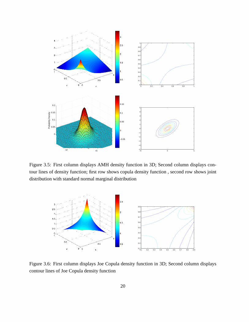
See figure 3.5 clearly shows that a AMH dependence structure is asymmetric and the lower

tail is heavier than upper tail. Besides, its tail dependence coefficientλUλL = 0, so we can con-

clude that its upper tail is light tail and its lower tail is light tail or normal tail.

Joe CopulaForα ≥ 1,consider the copula,

CJoe(u, v) = 1− ((1− u)α + (1− v)α − (1− u)α)(1− v)α(1/α) (3.6)

, Forα = 1, the formula (3.4)reduces toΠ(u, v),which is independent copula. The Frank copula’s

dependence structure is asymmetric and its tail dependencecoefficients areλU = 2 − 21/α and

λL = 0,see Figure3.6. Since its upper tail is heavier than the lower tail(from the expression we

know that the larger isα, the heavier is the upper tail), if two variates of the electricity market

follow the clayton copula, they would have a larger probability of simultaneous booming than

simultaneous crashing.

Gaussian CopulaOne of the most usually used copula,in particularly for finance modeling,

is the bivariateGaussian copula.Its formula is:

CGaussian(u, v) =∫ φ−1(u)

−∞

∫ φ−1(v)

−∞exp{−

x2 − 2ρxy+ y2

2(1− ρ2)}

dxdy

2π√

1− ρ2= φρ(φ

−1(u),φ−1(v)) (3.7)

Hereφ−1 is the inverse probability distribution function of the standard normal distribution,

meanwhileφρ is joint distribution function of a standard bivariate Gaussian with the correlation

coefficientρ,which is the sole parameter of Gaussian copula ,and yield in−1 < ρ < 1.

19

0 0.2 0.4 0.6 0.8 10

0.1

0.2

0.3

0.4

0.5

0.6

0.7

0.8

0.9

1

−2

0

2

−2

0

2

0

0.05

0.1

0.15

0.2

x1x2

Pro

babi

lity

Den

sity

−0.05

0

0.05

0.1

0.15

−5 0 5−5

−4

−3

−2

−1

0

1

2

3

4

5

Figure 3.5: First column displays AMH density function in 3D; Second column displays con-

tour lines of density function; first row shows copula density function , second row shows joint

distribution with standard normal marginal distribution

0.1 0.2 0.3 0.4 0.5 0.6 0.7 0.8 0.90.1

0.2

0.3

0.4

0.5

0.6

0.7

0.8

0.9

Figure 3.6: First column displays Joe Copula density function in 3D; Second column displays

contour lines of Joe Copula density function

20

See Figure 3.7 clear displays that a Gaussian dependence structure is symmetric,If two vari-

ates of the electricity market follow the Gaussian copula, they would have the same probability

of simultaneous crashing than simultaneous booming.Morever, its tail dependence coefficient

λU = λL = 0, so we say that the tail of Gaussian copula is normal tail.

Indeed, a gaussian dependence structure withρ > 0 means that the variants are positive

quadrant dependent, similarly, ifρ < 0 the variants are negative quadrant dependent.

For example, if we takeρ < 0 for the electricity future price, it displays that there islarger

probability for variants to move in the reserve way, which means that if one variate boom, the

other variate shows higher probability to crash.

NOTE: The variates of Gaussian copula are just multivariate normal distribution if marginal

are normal distributed.

t Copula The bivariate Student t.s copula,Ctρ,υ, whereυ is degrees of freedom, defined

as

Ct(u, v) =∫ t−1

υ (u)

−∞

∫ t−1υ (v)

−∞(1+

x2 − 2ρxy+ y2

υ(1− ρ2))

dxdy

2π√

1− ρ2= tρ,v(t

−1υ (u), t−1

υ (v)) (3.8)

Heret−1υ is the inverse probability distribution function of the student t distribution,and the cor-

relation coefficient ρ,which is one parameters of Student t’s copula ,and yield in−1 < ρ <

1.Student.s copula, with the corresponding picture for the Gaussian copula (Figure 3.8)It is

easy to notice that Student t copula shows more observationsin the tails than the Gaussian

one.Morever, its tail dependence coefficient λU = λL = 0, so we say that the tail of Student

t’s copula is nearly normal tail.

HH1 Copula For the parameterα1 > 0,α2 ≥ 1, HH1 is defined as:

Cα1,α2HH1 (u, v) = (1+ ((u−α1 − 1)α2 + (v−α1 − 1)α2)1/α2)−1/α1 (3.9)

The HH1 copula’s dependence structure is asymmetric, and itcharacterize both tails. The

21

0.1 0.2 0.3 0.4 0.5 0.6 0.7 0.8 0.9

0.1

0.2

0.3

0.4

0.5

0.6

0.7

0.8

0.9

rho=0.5

0.0

0.5

1.00.0

0.5

1.0

0

50

100

0.1 0.2 0.3 0.4 0.5 0.6 0.7 0.8 0.9

0.1

0.2

0.3

0.4

0.5

0.6

0.7

0.8

0.9

rho=0.95

−4−2

02

4

−4

−2

0

2

40

0.1

0.2

0.3

0.4

0

0.05

0.1

0.15

0.2

0.25

0.3

0.35

−3 −2 −1 0 1 2 3−3

−2

−1

0

1

2

3

Figure 3.7: First column displays density function in 3D with ; Second column displays con-

tour lines of density function ; first row shows Gaussian copula density function with rho=0.95,

second row shows Gaussian copula density function with rho=-0.95, third row shows joint dis-

tribution with standard normal marginal distribution

22

0

0.5

1

0

0.5

10

0.5

1

1.5

2

2.5

3

u1u2 0

0.5

1

1.5

2

2.5

0.1 0.2 0.3 0.4 0.5 0.6 0.7 0.8 0.9

0.1

0.2

0.3

0.4

0.5

0.6

0.7

0.8

0.9

−2

0

2

−2

0

2

0

0.05

0.1

0.15

0.2

x1x2

Pro

babi

lity

Den

sity

−0.05

0

0.05

0.1

0.15

−3 −2 −1 0 1 2 3−3

−2

−1

0

1

2

3

Figure 3.8: First column displays t copula density functionin 3D; Second column displays con-

tour lines of density function; first row shows t copula density function , second row shows joint


23

0.1 0.2 0.3 0.4 0.5 0.6 0.7 0.8 0.90.1

0.2

0.3

0.4

0.5

0.6

0.7

0.8

0.9

Figure 3.9: First column displays HH1 Copula density function in 3D; Second column displays

contour lines of HH1 Copula density function

density function figure of copula is centralized closely to the lineu = v, see Figure 3.9. Mean-

while, the tail dependence coefficients areλU = 2− 21/α2 andλL = 21/α1α2.

Galambos CopulaForα ≥ 0,consider the copula,

Cgalambos(u, v) = uve−((−log(u))−alpha+(−log(v))−alpha)−1/α(3.10)

see Figure 3.10 displays that the Galambos copula’s dependence structure is asymmetric and its

tail dependence coefficients areλU = 2−1/α andλL = 0.

3.3 Extreme Value Copulas

A copula is named to be an extreme value copula if for alls> 0 the scaling property.C(us, vs) =

(C(u, v))s for ∀u, v ∈ I .

Extreme Value copula are max-stable, which means if (X1,Y1), (X2,Y2), ...(XN,YN) are in-

dependent identically distribution random pairs from an Extreme Value copula C. andM =

{X1,X2, ...,XN} andW = {Y1,Y2, ...,YN}, so the copula for (M,W) is also a copula, consider the

following formula:

CExtremeValue(u, v) = elog(uv)A(log(u)log(v)/log(uv)) (3.11)

24

0.2 0.3 0.4 0.5 0.6 0.7 0.8 0.90.2

0.3

0.4

0.5

0.6

0.7

0.8

−150 −100 −50 0 50 100 150 200

−150

−100

−50

0

50

100

150

200

250

Figure 3.10: First column displays density function in 3D; Second column displays contour lines

of density function; first row shows Galambos copula densityfunction , second row shows joint


25

,

where the function A is the dependence function.

3.4 FrWWWchetõõõHoeffding Family

Definition 3.4.1. Letα,β ∈ I with α + β ≤ 1 and define

Cα,β(u, v) = βM(u, v) + (1− α − β)Π(u, v) + αW(u, v), (3.12)

this expression with two unknown parameter is called a Frechet Hoeffding Family.

Now set the correlation of the Frechet Hoeffding Family is

ρ = α − β

.With the conditionα = 0, it is negative quadrant dependence, while the conditionβ = 0, it is

positive quadrant dependence.

26

Chapter 4

Sampling Random Number for Copulas

Models

After understand the definition and important properties ofseveral copulas.In this chapter

we will present the method how to generate random variables whose dependence structure is

define by a copula.

4.1 The Generation Method

The joint density function is bounded,f (x, y) ≤ N ,then a random variate (X,Y) from the

this dependence structure may be created as follow:

1.Generate two uniform distributed random variablesε, ζ from a certain box domain;

2. generate a uniform variable,ǫ from [0,N];

3. if f(ε, ζ)≤ ǫ,accept (ε, ζ) to the data sets, otherwise go back to 1step.

But C(u,v)may not bounded, in this case we may change the uniform marginal distribution,

for example as Gaussian copula, consider two random variables with normal marginal distribu-

tions,then

F(x, y) = C(φ(x),φ(y))

27

.

and its density function is given by :

f (x, y) =∂

∂u∂vF(x, y) =

∂

∂u∂vC(φ(x),φ(y)) = c((φ(x),φ(y))φ(x)φ(y),

,

wheredφ(x)/dx= φ(x).

Simulation in the n dimension conditions is given as follow:

1.Generate n independent random variatesz= (z1, z2, ..., zn) from N(0, 1);

2. Setui = φ(xi) with i = 1, 2, . . . , n and whereφ denotes the univariate standard normal

distribution function;

3.(u1, ..., un)∗ = (F1(t1), ..., Fn(tn))∗ whereFi denotes theith margin.

The Student T copula is also similar to estimate.

Another method to generate random variables from a chosen copula is formulated by using

a conditional approach (conditional sampling). Let us explain this concept in a easy way, under

the assumption of that a bivariate copula in which all of its parameters are known. The task is

to generate pairs (u, v) of observations of [0, 1] uniformly distributed r.v.s U and V whose joint

distribution function is C. To reach this, we will cite the conditional distribution.

Let cu define the conditional distribution function for the randomvariables V at the given value

u of U,

cu(V) = Pr(V ≤ v | U = u)

From(2.1), and because the density function of a uniform distribution constantly equal to

one, we have

cu(V) = Pr[V ≤ v | U = u] =∫ v

−∞

f (y, u)fX(U)

dx=∫ 0

vc(u, v)dy=

∂

∂xC(x, y) |x=u= Cu(u, v) (4.1)

whereCu(u, v) is the partial derivative of the copula C. We know thatcu(V) is a non-decreasing

28

function and exists for allv ∈ I .

With the result(4.1), we have the following conditional distribution method to generate the

data, as follows:

1. Generate a uniformly distribution random variables (η ∈ I );

2. Generate (V | U = η) from the conditional copula;

3. Now (η, (U | V = η)) will be a random variate with the expected distribution.

From above bivariate generation processing, the general procedure in a multivariate setting

is as follows:

1. DefineCi = C(F1, F2, ..., Fi, 1, 1, ..., 1) for i = 2, 3, ..., n.

2. GenerateF1 from the uniform distribution U(0, 1).

3. Next, generateF2 from C2(F2 | F1).

4. More generally, generateFn from Cn(Fn|F1, ..., Fn−1).

4.2 The Generation Random Numbers of some examples

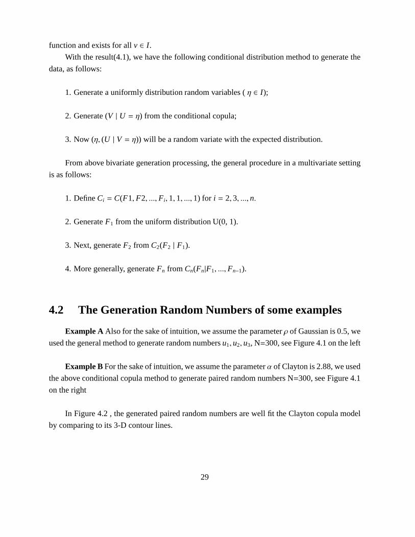
Example A Also for the sake of intuition, we assume the parameterρ of Gaussian is 0.5, we

used the general method to generate random numbersu1, u2, u3, N=300, see Figure 4.1 on the left

Example BFor the sake of intuition, we assume the parameterα of Clayton is 2.88, we used

the above conditional copula method to generate paired random numbers N=300, see Figure 4.1

on the right

In Figure 4.2 , the generated paired random numbers are well fit the Clayton copula model

by comparing to its 3-D contour lines.

29

05

1015

00.20.40.60.81−5

0

5

X1X2

X3

0 0.2 0.4 0.6 0.8 10

0.1

0.2

0.3

0.4

0.5

0.6

0.7

0.8

0.9

1Clayton Copula, α = 2.88

U1

U2

Figure 4.1: First column displays generated Gaussian Copula in 3D; Second displays generation

of random variables from clayton copula

4.3 Robust Estimation of Significant

The bootstrap method would be used to test the goodness of fit the models.

The details is as follow:

1. Generate pairs (η, ξ) from model of data sets sample size;

2. find empirical copula function from the generated data;

3. calculate the maximum distance(KS) of the empirical copula to the model copula (See

Appendix );

4. repeat the above procedure 1000 times;

5. plot the empirical distribution function of the observedmaximum distances.

Finally, using the empirical distribution function of maximum distance, estimate p-values

for the maximum distance statistics may be found.

30

Chapter 5

Data exploration and Investigation

Data sets process electricity futures and related fuel future returns. And all these electricity

futures are affected by these fuel prices, when modelling the price processan asset on a true

market, normally the logreturns of the asset are consideredas i.i.d. According to the distribution

of electricity future price, the investment policy of electricity price is reflected in the structure of

its future price. So in order to avoid crashes, the futures should display negative dependence, on

the contrary, to reach maximum profit, the futures should display positive dependence.

5.1 Data exploration

To investigate the different dependence structures of electricity futures of years 2007-2010

on the real-world markets,long term data of electricity future price is provided bySKM Market

Predictor and help from Alain Angeralides as an electricity price trader at Bixia Energy Man-

agement AB.

Since the length of very future price is different, moreover, pair of them must be picked on a same

day,I divide them into two group , group one is electricity future price in 2011(ENYOR) , Coal fu-

ture price and Co2 emission price; the other is the same electricity future price in 2011(ENYOR)

, Gas future price and Oil future price. Which is also for the sake of fitting three dimension

copulas for the data sets.

First I fit a bivariate copula for these two group data, that means there are four pairs variates;

then I use the pair-copula method to fit a three dimension copula.

Bachelier-Samuleson Black-Scholes Model

In many model of stock return in the financial market, Bachelier-Samuleson Black-Scholes

31

Model is most used, which gives the stock value at time t as thesolution to the stochastic differ-

ential equation

dS(t) = (µ +σ

2)S(t)dt+ σS(t)dBt, (5.1)

whereBt is brownian motion.

The solution to (5.1) is

S(t) = S(0)eµt+σBt , (5.2)

whereS(0) is the return value at the starting time,µ is the drift coefficient andσ2 > is the volatil-

ity.

Consider the logreturn,X(t), of the return value, the data set becomes driven easily by the

increments of a Brownian motion:

X(t) = log(S(t + ∆)) − log(S(t)) = log(eµ(t+δ)+σBt+δ−µt−σ Bt) = µδ + σ(Bt+δ − Bt)

,

whereδ is time interval between sampling points. Therefor, for theBachelier-Samuleson

Black-Scholes Model the logreturn of stock values are the increments of an Brownian motion,

and they stationary and independent.

Filtering of Data

By examining data sets it can be checked that the volatility is not constant, so Bachelier-

Samuleson Black-Scholes Model is appropriate. To avoid this property of a financeial market we

introduce a devolzatilization of data set. One may generalize this Bachelier-Samuleson Black-

Scholes Model by(5.1) but substituting brownian motion by noise process a Levy processLt,i.e.

dS(t) = (µ +σt

2)S(t)dt+ σtS(t)dLt, (5.3)

The logreturnXt of the electricity future price,ifσt moves slowly compared toLt,

32

Xt = log(St) − log(St−∆) = log(eµζ+σtLt−σt−∆Lt−∆) = µ∆ + σtCt (5.4)

,

whereδ is time interval between sample point. The devolatlized logreturnsAt is a random

walk independent of the time changing volatility

At =Xt − µ∆σt

(5.5)

By devolatilizing the changing volatility, the data is madeindependent of market change. see

Nadaraya(1964) and Watson(1964).

Statistical Investigation of Data Sets We firstly present basic statistics of the logreturn

series of electricity futures and fuel(coal, gas, oil,co2 allowance) futures of Bixia Energy Energy

Management AB.

logreturn series mean covariance

ENOYR. 7.5015e-05 2.3503e-04

COAL. 7.9514e-04 3.6500e-04

CO2. 5.3195e-04 6.6712e-04

GAS. 2.6422e-04 2.3856e-04

OIL. 2.6788e-04 3.3383e-04

Table 5.1: Statistics for above five logreturn series in the period from 08-Jan-2007 to 25-Oct-

2010 with N=907

From Table 5.1, we calculate the first two empirical moments of the logreturns of electricity

futures and other four fuel futures.

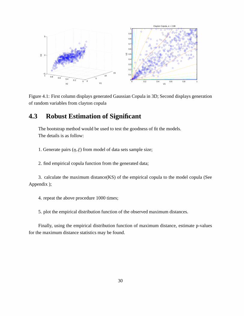
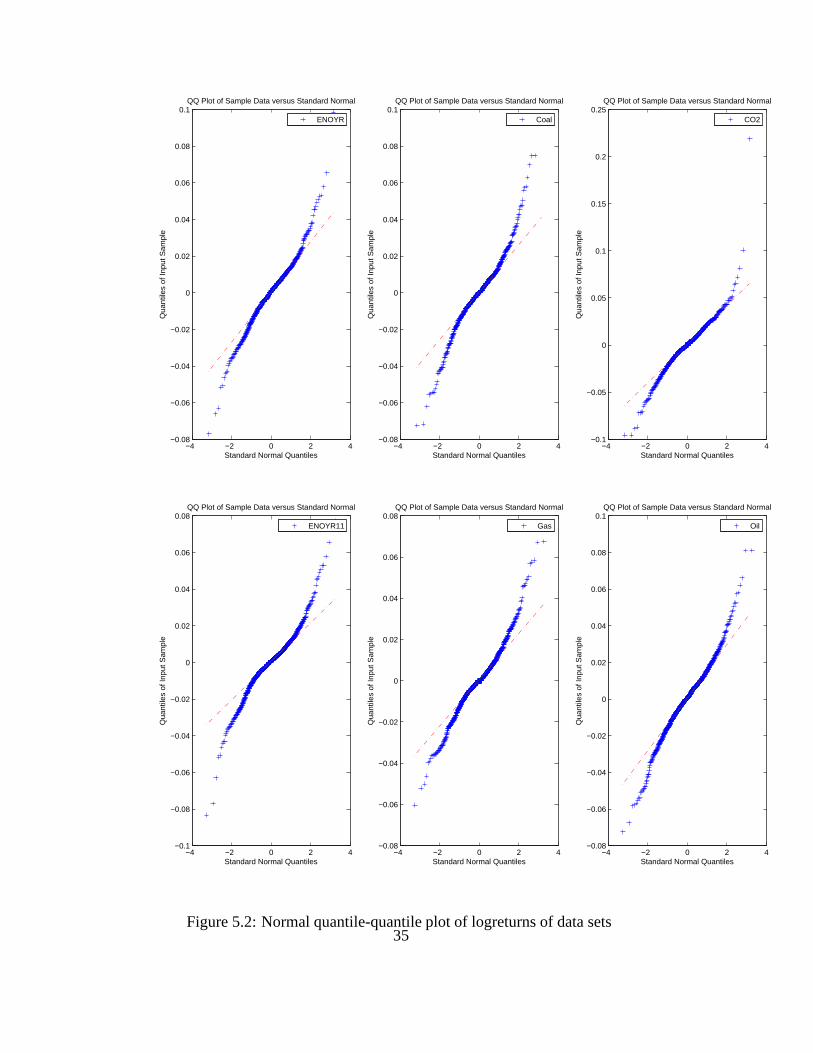
From observation of Figure 5.1 & 5.2, we see that all of these data sets have non-normal

distribution and most of them display heavy tails exceptCO2.

Also from Figure 5.3, it is obvious that the logreturns are time depemdent, the data is in

crashed dependency structure,and also with negative dependent of variates. Which is means that

33

0 100 200 300 400 500 600 7000

50

100

150

200

250

ENOYRCOALCO2

0 100 200 300 400 500 600 700 800 900 100020

40

60

80

100

120

140

160

ENOYRGASOIL

100 200 300 400 500 600

−0.06

−0.04

−0.02

0

0.02

0.04

0.06

0.08

ENOYR

100 200 300 400 500 600

−0.06

−0.04

−0.02

0

0.02

0.04

0.06

0.08

COAL

100 200 300 400 500 600

−0.05

0

0.05

0.1

0.15

0.2

CO2

100 200 300 400 500 600−0.08

−0.06

−0.04

−0.02

0

0.02

0.04

0.06

ENOYR

100 200 300 400 500 600

−0.06

−0.04

−0.02

0

0.02

0.04

0.06

GAS

100 200 300 400 500 600

−0.06

−0.04

−0.02

0

0.02

0.04

0.06

0.08

OIL

−0.1 0 0.1 0.2 0.30

100

200

300ENOYR

−0.1 −0.05 0 0.05 0.10

100

200

300COAL

−0.2 0 0.2 0.4 0.60

100

200

300CO2

−0.1 −0.05 0 0.05 0.10

100

200

300

400ENOYR

−0.1 −0.05 0 0.05 0.10

100

200

300

400GAS

−0.1 −0.05 0 0.05 0.10

100

200

300

400OIL

Figure 5.1: At top stock prices from 08-Jan-2007 to 25-Oct-2010 ,in the middle logreturn values

in the same time period, at the bottom plots histogram of logreturns of data sets

34

−4 −2 0 2 4−0.08

−0.06

−0.04

−0.02

0

0.02

0.04

0.06

0.08

0.1

Standard Normal Quantiles

Qua

ntile

s of

Inpu

t Sam

ple

QQ Plot of Sample Data versus Standard Normal

ENOYR

−4 −2 0 2 4−0.08

−0.06

−0.04

−0.02

0

0.02

0.04

0.06

0.08

0.1


Qua

ntile

s of

Inpu

t Sam

ple


Coal

−4 −2 0 2 4−0.1

−0.05

0

0.05

0.1

0.15

0.2

0.25


Qua

ntile

s of

Inpu

t Sam

ple


CO2

−4 −2 0 2 4−0.1

−0.08

−0.06

−0.04

−0.02

0

0.02

0.04

0.06

0.08


Qua

ntile

s of

Inpu

t Sam

ple


ENOYR11

−4 −2 0 2 4−0.08

−0.06

−0.04

−0.02

0

0.02

0.04

0.06

0.08


Qua

ntile

s of

Inpu

t Sam

ple


Gas

−4 −2 0 2 4−0.08

−0.06

−0.04

−0.02

0

0.02

0.04

0.06

0.08

0.1


Qua

ntile

s of

Inpu

t Sam

ple


Oil

Figure 5.2: Normal quantile-quantile plot of logreturns ofdata sets35

Figure 5.3: Copula density function of time dependence structure for electricity future price in

2011

data sets in not individual independent, this means that themethod to use maximum likelihood

to estimate the parameter of copula may not be accurate.

5.2 Find fitted bivariate copula for data sets

The numerical method is to calculate the minimum Kolmogorov-Smirnov distance between

fitted copulas and empirical copula, which of the distance value is save in Table 5.2,the five

devolatilized logreturn series of electricity future price of 2011 (ENYOR), Coal,CO2(emission

price), Gas and Oil, labeled asFi for i ∈ 1, 2, 3, 4, 5. Now we look back for the dependence

structure for pairF1&F2 ,...,F1&F4. Electricity and Coal ,Gas, Oil all have higher crash depen-

dence than boom dependence, excepet Electricity andCo2 are higher boom dependence.See the

empirical density function in 3D and its cumulative function contour shown in the Figure 5.4

For the various copulas and each pair of logreturn series, bycalculating the minimum

KS distance between the empirical copulas and theoretical models, the copula’s parameters are

searched. And Figure 5.5 plots of KS distance of copulas compared with the empirical copulas

show that Gumbel Survival copula is larger than other copulas, which means there is a lower tail

dependence in our data set.

The p-value should be calculated to see whether Gumbel survial copula is the suitable cop-

36

0.2 0.4 0.6 0.8 1.0

0.2

0.4

0.6

0.8

1.0

0.2 0.4 0.6 0.8 1.0

0.2

0.4

0.6

0.8

1.0

0.2 0.4 0.6 0.8 1.0

0.2

0.4

0.6

0.8

1.0

0.2 0.4 0.6 0.8 1.0

0.2

0.4

0.6

0.8

1.0

Figure 5.4: Fist row displays empirical density copula ofF1&F2(ENYOR and Coal), the left con-

tours corresponding empirical cumulate function; Second row displays empirical density copula

of F1&F3 (ENYOR and CO2), the left contours corresponding empiricalcumulate function;

Third row displays empirical density copula ofF1&F4 (ENYOR and Gas), the left contours cor-

responding empirical cumulate function; Forth row displays empirical density copula ofF1&F5

(ENYOR and Oil), the left contours corresponding empiricalcumulate function

37

Copula ENYOR&COAL ENYOR&CO2 ENYOR&GAS ENYOR&OIL

Gaussian ρ = 0.807,D = 0.048 ρ = 0.429,D = 0.042 ρ = 0.328,D = 0.053ρ = 0.642,D = 0.051

Clayton α = 1.948,D = 0.057 α = 1.545,D = 0.046 α = 0.973,D = 0.049α = 0.856,D = 0.052

Clayton S urvivalα = 0.972,D = 0.061 α = 1.457,D = 0.054 α = 1.362,D = 0.064α = 1.221,D = 0.059

Frank α = 2.457,D = 0.051 α = 1.753,D = 0.052 α = 1.524,D = 0.048α = 2.390,D = 0.063

Frank S urvival α = 2.457,D = 0.051 α = 1.657,D = 0.051 α = 1.524,D = 0.048 α = 2.40,D = 0.063

AMH α = 0.898,D = 0.058 α = 0.917,D = 0.049 α = 0.872,D = 0.050α = 0.946,D = 0.053

AMH S urvival α = 0.903,D = 0.062 α = 0.900,D = 0.065 α = 1.000,D = 0.060α = 0.916,D = 0.061

Gumbel α = 2.438,D = 0.057 α = 2.712,D = 0.054 α = 1.306,D = 0.042α = 1.672,D = 0.052

Gumbel S urvivalα = 2.645,D = 0.043 α = 2.60,D = 0.049 α = 1.581,D = 0.050α = 2.306,D = 0.048

Joe α = 1.257,D = 0.054 α = 1.116,D = 0.057 α = 1.357,D = 0.058α = 1.897,D = 0.055

Joe S urvival α = 1.306,D = 0.049 α = 1.004,D = 0.055 α = 1.420,D = 0.053α = 1.669,D = 0.051

Galambos α = 0.916,D = 0.056 α = 0.971,D = 0.062 α = 0.957,D = 0.053α = 0.857,D = 0.058

Galabos S urvivalα = 0.930,D = 0.063α = 0.892,D = 0.0514α = 0.780,D = 0.065α = 0.910,D = 0.058

Table 5.2: Minimal KS distances and copula parameter value for paired data

ula. During the calculation of p-values for these four pairs,F1&F2 ,..., F1&F4, we found that

Gumbel Survival is not a good model , since all the p-value aresmaller than 5%

5.3 Fitting multi-dimension copula for data

We are going to show how to do modeling for multivariate data with a series of simple

constructing modules named pair-copula. This constructing method displays a new way to build

complex multivariate correlation model, which is similar to classic rank model; the key here is

to build certain structure models with conditional independent simple structures, which is based

on the Joe, Bedford and Cooke’s work.

5.3.1 pair-copula for high dimension data sets

A pair-copula model is proposed to model the high-dimensional dependency structure of fi-

nancial market returns, for example: in my thesis, is electricity future price and its corresponding

future price.

Considering a vectorX = (X1, ...,Xd) has the follow joint density distribution function

([Bedford and Cooke, 2002])

38

G Cl ClS Fr FrS A AS Gu GuS Jo JoS Ga GaS0

0.01

0.02

0.03

0.04

0.05

0.06

0.07

0.08

0.09

0.1

Gauss Clayton Frank AMH Gumbel Joe Galambos

ENY&COALENY&CO2ENY&GASENY&OIL

Figure 5.5: KS distance of copulas compared with the empirical copulas

f (x1, ..., xd) = f (xd) ∗ f (xd−1 | xd) ∗ f (xd−2 | xd−1, xd) ∗ ... f (x1 | x2, ..., xd); (5.5)

According to [Sklar, 1959], every multivariate distributions F with marginal densitiesF1(x1), ..., Fd(xd)

can be written as

F(x1, ..., xd) = C(F1(x1), ..., Fd(xd)) (5.6)

Therefore, the copula in (5.6) can be written as

C(u1, ..., ud) = F−1(F1(u1), ..., Fd(ud)) (5.7)

The general formula is given by :

f j|i(xj | xi) =f (xi, xj)

fi(xi)= ci j (Fi(xi), F j(xj)) ∗ f j(xj) (5.8)

which is easy handy to draw to high dimension.

Now we set up 3-dimensional density function. Any such function can be written in this

form:

f (x1, x2, x3) = f1(x1) ∗ f2|1(x2 | x1) ∗ f3|1,2(x3 | x1, x2) (5.9)

39

where the factorization is unique up to a relabeling of the variables.

Note that the second term on the right hand sidef2|1(x2 | x1) can be written in terms of a pair-

copula and a marginal distribution using (5.8). Since the last term f3|1,2(x3 | x1, x2) we can pick

one of the conditional variables, say x2, and use a form similar to (5.9) to arrive at

f3|12(x3 | x1, x2) = c13|2(F1|2(x1 | x2), F3|2(x3 | x2)) ∗ f3|2(x3 | x2). (5.10)

This decomposition involves a pair-copula and the last termcan then be decomposed into

another pair-copula, using (5.8) again, and a marginal distribution. This yields, for a three di-

mensional density, the full decomposition

f (x1, x2, x3) = f1(x1)∗c12(F1(x1), F2(x2))∗ f2(x2)∗c31|2(F3|2(x3 | x2), F1|2(x1 | x2))∗c23(F2(x2), F3(x3))∗ f3(x3).

(5.11)

The follow step we will use above formula to fit our data sets, which is divide into two

groups:group 1 for electricity price (F1), coal (F2) andCO2 (F3); group 2 for electricity price

(F1) , gas (F4) and oil(F5).

5.3.2 Fit copulas for three dimension data sets

It is similar numerical method with two dimension model, which is also to calculate the

minimum Kolmogorov-Smirnov distance between fitted copulas and empirical copula, which of

the distance value is plotted in Figure 5.6 , the five devolatilized logreturn series of electricity

future price of 2011 (ENYOR), Coal,CO2(emission price), Gas and Oil, divided by two groups.

For the various three dimension copulas and each triple variates of logreturn series, by cal-

culating the minimum KS distance between the empirical copulas and theoretical models, the

copula’s parameters are searched. See Table 5.3

The p-value should be calculated to see whether there is a copula suitable. During the

calculation of p-values for these two groups, we found that there is no such a good model , since

all the p-value are far smaller than 5%

Because triple variates have more complex dependency structure, there is no single copula model

is fitted, then let us find its mixture one.

40

Cl ClS Fr FrS A AS Gu GuS Jo JoS Ga GaS0

0.01

0.02

0.03

0.04

0.05

0.06

0.07

0.08

0.09

0.1

Clayton Frank AMH Gumbel Joe Galambos

Group1Group2


Copula Group 1 Group 2

Clayton α = 2.971,D = 0.067α = 3.315,D = 0.066

Clayton S urvivalα = 1.842,D = 0.071α = 2.437,D = 0.074

Frank α = 8.421,D = 0.081α = 9.052,D = 0.072

Frank S urvival α = 7.945,D = 0.075α = 8.859,D = 0.071

AMH α = 0.997,D = 0.064α = 0.893,D = 0.059

AMH S urvival α = 0.972,D = 0.067α = 0.912,D = 0.073

Gumbel α = 2.654,D = 0.051α = 2.720,D = 0.052

Gumbel S urvivalα = 2.793,D = 0.055α = 2.809,D = 0.058

Joe α = 2.251,D = 0.064α = 3.105,D = 0.068

Joe S urvival α = 2.753,D = 0.059α = 2.801,D = 0.065

Galambos α = 0.881,D = 0.058α = 0.901,D = 0.062

Galabos S urvivalα = 0.926,D = 0.066α = 0.912,D = 0.058

Table 5.3: Minimal KS distances and copula parameter value for triple variates data

41

Chapter 6

Mixture Copulas for bivariate copulas and

multivariate copulas

6.1 Mixture copulas for bivariate copulas

Simulation Method: First, we estimate the association parameters by finding the minimum

Kolmogorov-Smirnov distance of between the empirical copula and every theoretical copula

(Table 5.2). Second, we use the minimum Kolmogorov-Smirnovdistance to estimate the shape

parameters of the mixture copula, which is the coefficient of every single copula.

From Nelsen (1999): copula after mixing is still a copula. After simulating the copulas

that estimate lower tail, upper tail and central dependenceand mixing them together in mixing

copula,we finally found our model copula. We mixed of three copulas, Frank copula , Gumbel

Survival copula and Clayton copula. The results are shown inTable 6.1

Cmix(u, v) = β1C f rank(u, v, α1) + β2Cgumbelsurvival(u, v, α2) + β3Cclayton(u, v, α3) (6.1)

whereα = (α1, α2, α3) are association parameters in the mixture copula which effect the

degree of dependence, andβ = (β1, β2) are weight parameters in the mixture copula which reflect

the shape dependence structures. Follows that choosingβ1,β2,β3 ∈ [0,1], β3 =1-(β1 + β2) with

β1 + β2 ≤ 1. See Figure 6.1, plots some mixture copula density function and its contour with

different values of vectorα andβ.

Finally we need to test goodness-of- fit of the model I found, may be specified in two ways,

42

0.1 0.2 0.3 0.4 0.5 0.6 0.7 0.8 0.90.1

0.2

0.3

0.4

0.5

0.6

0.7

0.8

0.9

0.1 0.2 0.3 0.4 0.5 0.6 0.7 0.8 0.90.1

0.2

0.3

0.4

0.5

0.6

0.7

0.8

0.9

Figure 6.1: At top displays the mixture copula density function with β1 = 0, β2 = 1/3, β3 = 1/2

andα1 = 1.94,α2 = 8.15,α3 = 2.48 , at the bottom displays the mixture copula density function

with β1 = 1/3,β2 = 1/3,β3 = 1/3 andα1 = 1.94,α2 = 8.15,α3 = 2.48

43

ENYOR&COAL ENYOR&CO2 ENYOR&GAS ENYOR&OIL

α1 2.457 1.753 1.524 2.390

α2 2.645 2.60 1.581 2.306

α3 1.947 1.545 0.973 0.856

β1 0.013 0.526 0.273 0.115

β2 0.399 0.415 0.439 0.356

β3 0.588 0.069 0.302 0.529

Table 6.1: parameter value of mixture copula for different paired data

0.013 0.016 0.019 0.022 0.025 0.028 0.031 0.034 0.037 0.0400

0.1

0.2

0.3

0.4

0.5

0.6

0.7

0.8

0.9

1

KS Distance

F(x

)

Empirical CDF


one is a Kolmogorov-Smirnov test , the other is chi-square test.

For the first method: the calculated Kolmogorov-Smirnov distance (greatest distance) be-

tween fitted mixture copula and empirical distribution for every pair of data sets, that isD12 =

0.043,D13 = 0.038,D14 = 0.036. Then using the bootstrap method was used o find the approxi-

mate p-value of the generated data sets from the copula model, the results plots in Figure 6.2 and

which shows that all the distanceD12 = 0.043,D13 = 0.038,D14 = 0.036 are too large to reject

the fitted mixture model.

For the second method is a chi-square test, thep-valueof paired future price of ENYOR

and Coal, ENYOR and Gas, ENYOR and Oil is larger than 5%, so accept the fitted model, which

44

means my mixture model fits real data sets as well.

Compared with the single Clayton Copula, my mixture copulasis more precise. See the

comparison of results in Table 6.2.

ENYOR&COAL ENYOR&CO2 ENYOR&GAS ENYOR&OIL

Cmixture 0.156 0.029 0.573 0.108

Cgumbelsurvial 8.43e-04 2.759e05 1.306e05 7.672e04

Table 6.2: comparison of p-value between mixture copula andclayton copula

6.2 Mixture copulas for multivariate copulas

Using the same method to find mixture copulas for triple variates of real world (u, v, z) fi-

nally we mixed of three copulas, Clayton copula , Jeo Survival copula and AMH copula. The

results are shown in Table 6.3

Cmix(u, v, z) = β1Cclayton(u, v, z, α1) + β2CJoesurvival(u, v, z, α2) + β3CAMH(u, v, z, α3) (6.2)

Group 1 Group 2

α1 2.971 3.315

α2 2.753 2.801

α3 0.997 0.893

β1 0.335 0.416

β2 0.399 0.573

β3 0.366 0.011

Table 6.3: parameter value of mixture copula for different paired data

This time chi-square test is used, thep-valueof triple future price ofGroup1&Group2, are

both larger than 5%, which isp = 0.059 andp = 0.106 so accept the fitted model, which means

this mixture model fits real data sets as well.

45

Chapter 7

Conclusion

The assumption of dependence structures of variates is not always true. From the empirical

copulas, we know that the dependence structure of real worlddata is more complex. Usually,

tail dependence is stronger than in central regions of data.Moreover, unlike the multivariate

Gaussian distributions, the real market has asymmetric dependence, which always cline to crash

dependency. Therefore, the linear correlation is suitablefor the fitting Gaussian Processes, but

not suitable in the real market, as the data come from more complex distributions. In one word,

correlation cannot reflect the dependence in the electricity market, and the previous chapters have

shown that copula models describe the dependence much better, especially the mixture copulas.

We need to mention that under 2D conditions, we could assume that data sets come from a

Gumbel Survival copula, but we cannot assume that they are jointly Gaussian distributed, other-

wise, it may lead to critical mistake, since we must considerthe true data distribution is heavy

lower tail, that is crash dependence. Mixture copula can fit the real data quite well, since its

weight parameter effect shape of dependence, besides association parameters reflect its depen-

dence degree. For the 3D case, we can also use the copula generator to derive the copula function

of triple variates, however, the pair copula method appliedin this thesis is more comprehensive

and easy to apply.

46

Appendices

47

.1

The Kolmogorov -Smirnov distance is the gretest distance between the empirical distribu-

tion and a theoretical distribution for the data sets,i.e. in the term of copulas:

DKS = Max | Cemp(u, v) −Ctheory(u, v) |

for u, v ∈ [0, 1], whereCemp is the empirical copula andCtheory is the theoretical copula.

.2

A p-value of 0.05, for instance, means that you would have only 5% chance of eliciting the

sampling being tested if the null hypothesis was actually true. A p-value is close to zero signals

that the null hypothesis is false, otherwise, accept the null hypothesis,where 0.05 is a typical

threshold used in the real world test.

In this thesis I calculate a p-value by the chi-square statistics test to check whether copula

models fit the loagreturn data sets.

The chi-square statistic test of m boxes is given that,

χ2 =

m∑

i=1

(Oi − Ei)2

Ei

whereOi is observed frequency,andEi is expected frequency .

Ei = n[C(ui , vi) −C(ui−1, vi) −C(ui , vi−1) +C(ui−1, vi−1)]

Hereui > ui−1, vi > vi−1,u0 = v0 = 0 anduk = vk = 1 must hold.

48

Bibliography

[1] Friedrich Schmid, : Measuring Conditional Dependence. http://www.case.hu-

berlin.de/events/Archive/Workshops/Copulae/talks/Schmid.pdf, 2007.

[2] Etienne Cuvelier, Monique Noirhomme-Fraiture,: Clayton copula and mixture decompo-

sition. www.fundp.ac.be/pdf/publications/55680.pdf , 2005.

[3] Leslie Lamport, Yuri Goegebeur: Modelling dependence through copulas.

www.econ.kuleuven.be/insurance/pdfs/LectureNotesUbatuba.pdf, 2003.

[4] Claudia Kluppelberg,Gabriel Kuhn,: Copula Structure Analysis for High-dimensional

Data.

www-m4.ma.tum.de/Papers/Klueppelberg/copstruc070128.pdf, 2009.

[5] Xianling Ren , Shiying Zhang,: Copula function selection criterion based on nonparame-

teric kernel density estimation.

http://www.cqvip.com/qk/96188x/201001/1001258282.html, 2010.

[6] Florence Wu, Emiliano A. Valdez,: Simulating Exchangeable Multivariate Archimedean

Copilas and its Applications.

http://wwwdocs.fce.unsw.edu.au/actuarial/research/papers/2006/SimulatingArchimedean

Copulas.pdf, 2006.

[7] Jan Lennartsson, Miu Shu: Copula Dependence Structure on Real Stock Markets. Master

Thesis, Chalmers University of Technology,

http://www.math.chalmers.se/ palbin/janmin.pdf 2005

[8] Alain Angeralides,Ottmar Croniez: Modelling electridity prices with Ornstein-Uhlenbeck

processes. Master Thesis, Chalmers University of Technology,

http://www.math.chalmers.se/ palbin/CorrectedThesis30Aug.pdf

49

[9] Joe, H.: Families of m-variate distributions with given margins and m(m− 1)/2 bivariate

dependence parameters.. Schweizer, B., and Taylor, M. D.,editors, Distributions with fixed

marginals and related topics, pages 120-141, 1996.

[10] Nadaraya,E.A.: On estimating regression. Theory of Probability and its Applications 9

141-142. 1964

[11] Nelssen,R.B.: A Introduction to Copulas. Springer, New York. 1999

[12] Umberto Cherubini,: Copula methods in finance. John Wiley & Sons Ltd, The Atrium,

Southern Gate, Chichester, West Sussex PO19 8SQ, England, 2004.

[13] Aas, Czado,: Pair-copula constructions of multiple dependence. Sonderforschungsbereich

386, Paper 487, 2006.

http://epub.ub.uni-muenchen.de/

[14] John H., J.Einmatl,: Estimating a Multidimensional Extreme-Value Distribution. Eind-

hoven University of Technology, The Netherland, 1993

http://arno.uvt.nl/show.cgi?f id = 14233

[15] Watson,G.S.: Smooth regression analysis. Sankhya, Series A 26, 359-372.

[16] Chatfield, C.:The Analysis of Time series an introduction. Chapman & Ha .

50

Modeling Dependence Structures in the Electricity Price ...

Documents

Transcript of Modeling Dependence Structures in the Electricity Price ...