Non-linear Demand and Price: An Empirical Analysis of the Brazilian Industrial Electricity...

Seediscussions,stats,andauthorprofilesforthispublicationat:http://www.researchgate.net/publication/276847758

Non-linearDemandandPrice:AnEmpiricalAnalysisoftheBrazilianIndustrialElectricityConsumption

ARTICLE·JANUARY2014

DOWNLOADS

8

VIEWS

3

2AUTHORS:

ClaudioR.Lucinda

UniversityofSãoPaulo

44PUBLICATIONS23CITATIONS

SEEPROFILE

FranciscoAnuattiNeto

UniversityofSãoPaulo

24PUBLICATIONS26CITATIONS

SEEPROFILE

Availablefrom:FranciscoAnuattiNeto

Retrievedon:15June2015

http://www.researchgate.net/publication/276847758_Non-linear_Demand_and_Price_An_Empirical_Analysis_of_the_Brazilian_Industrial_Electricity_Consumption?enrichId=rgreq-c670618f-bcda-4b0d-b2ea-5d203cb6e471&enrichSource=Y292ZXJQYWdlOzI3Njg0Nzc1ODtBUzoyMzA1NTk1NDg5NjQ4NjRAMTQzMTk4MTA4ODEzMA%3D%3D&el=1_x_2

http://www.researchgate.net/publication/276847758_Non-linear_Demand_and_Price_An_Empirical_Analysis_of_the_Brazilian_Industrial_Electricity_Consumption?enrichId=rgreq-c670618f-bcda-4b0d-b2ea-5d203cb6e471&enrichSource=Y292ZXJQYWdlOzI3Njg0Nzc1ODtBUzoyMzA1NTk1NDg5NjQ4NjRAMTQzMTk4MTA4ODEzMA%3D%3D&el=1_x_3

http://www.researchgate.net/?enrichId=rgreq-c670618f-bcda-4b0d-b2ea-5d203cb6e471&enrichSource=Y292ZXJQYWdlOzI3Njg0Nzc1ODtBUzoyMzA1NTk1NDg5NjQ4NjRAMTQzMTk4MTA4ODEzMA%3D%3D&el=1_x_1

http://www.researchgate.net/profile/Claudio_Lucinda?enrichId=rgreq-c670618f-bcda-4b0d-b2ea-5d203cb6e471&enrichSource=Y292ZXJQYWdlOzI3Njg0Nzc1ODtBUzoyMzA1NTk1NDg5NjQ4NjRAMTQzMTk4MTA4ODEzMA%3D%3D&el=1_x_4


http://www.researchgate.net/institution/University_of_Sao_Paulo?enrichId=rgreq-c670618f-bcda-4b0d-b2ea-5d203cb6e471&enrichSource=Y292ZXJQYWdlOzI3Njg0Nzc1ODtBUzoyMzA1NTk1NDg5NjQ4NjRAMTQzMTk4MTA4ODEzMA%3D%3D&el=1_x_6


http://www.researchgate.net/profile/Francisco_Anuatti_Neto?enrichId=rgreq-c670618f-bcda-4b0d-b2ea-5d203cb6e471&enrichSource=Y292ZXJQYWdlOzI3Njg0Nzc1ODtBUzoyMzA1NTk1NDg5NjQ4NjRAMTQzMTk4MTA4ODEzMA%3D%3D&el=1_x_4


http://www.researchgate.net/institution/University_of_Sao_Paulo?enrichId=rgreq-c670618f-bcda-4b0d-b2ea-5d203cb6e471&enrichSource=Y292ZXJQYWdlOzI3Njg0Nzc1ODtBUzoyMzA1NTk1NDg5NjQ4NjRAMTQzMTk4MTA4ODEzMA%3D%3D&el=1_x_6


Non-linear Demand and Price: AnEmpirical Analysis of the BrazilianIndustrial Electricity Consumption*

Claudio R. Lucinda**

Francisco Anuatti Neto***

Abstract

In this paper we proposed an econometric model for industrial electricity demand inBrazil. Differently from residential customers, industries in Brazil, in addition to pur-chasing energy and capacity, also face a tariff menu with Time of Use pricing. Each itemin this menu also has different components and price discrimination structure. All thesecharacteristics pose an empirical problem that, so far, has not been faced together in theliterature. This methodology was applied in a non-experimental micro data sample of646 large Brazilian industrial customers (with demands over 300 KW) between January2002 and December 2006. The results indicate demands for the various services (capacityand energy, separated between peak and non-peak hours) are price elastic, and at least inthe AZUL tariff, there is complementarity between energy and capacity in the differentperiods. Thus, policies on tariff structures based on assumptions of an inelastic aggregateelectricity demand could have effects that are quite different from what was intended.

Keywords: Tariff Menu; Price Discrimination; Discrete-Continuous Model.

JEL Codes: L51; L60.

*Submitted in September 2013. Revised in July 2014. The authors would like to thank allwho have helped with comments on the previous version of this paper.

**Associate Professor, Faculdade de Economia, Administracao e Contabilidade de RibeiraoPreto, Universidade de Sao Paulo, Brazil. Address: Av. Bandeirantes, 3900, Monte Alegre, ZIP14040-905. E-mail: [email protected]

***Professor Doutor (Assistant Professor), Faculdade de Economia, Administracao e Contabil-idade de Ribeirao Preto, Universidade de Sao Paulo, Brazil. Address: Av. Bandeirantes, 3900,Monte Alegre, ZIP 14040-905. E-mail: [email protected]

Brazilian Review of Econometricsv. 34, no 2, pp. 99–123 November 2014

Claudio R. Lucinda and Francisco Anuatti Neto

1. Introduction

The importance of efficient use of electricity is ever-growing, due to potentialemissions of green-house effect gases by the different energy sources. To makeelectricity use more efficient, it is especially important to develop electricity pricingpolicies – which demands a deep understanding of the demand for electricity, agood that cannot be stored and has variable demand through the day. If we addthat the belief that one of the possible technological paths for the auto industry isthe development of electric cars, the question of the use of electricity throughoutthe day is another motivation for the study of electricity demand. Additionally,the tariff’s design must deal with the fact that consumers respond to price signals,reorganizing their demand, both in total amount of electricity use and in terms ofusage throughout the day.

Usually electricity consumers are divided into two large categories – those thatdemand high voltage electricity (voltage above 2.3kV in Brazil) – and those thatdemand low voltage electricity. The residential and commercial consumers areusually in the second group, and the industrial consumers are more commonlyfound in the first group. The division between high and low voltage is also reflectedin terms of behavior of the group of consumers – both in terms of price sensitivityand in usage substitution throughout the day.

The greater part of empirical studies on the industrial demand of electricityin developing countries – where a large part of the additional demand will bein the next few years1 – ignores the fact that this consumer faces a tariff menuthat is much more complex than that of the residential consumers. The industrialconsumers, especially the large consumers in this category, not only face the needto buy energy and capacity, but also face different prices for energy and capacitypurchased at different times during the day.

The discussion on those tariff menus is especially important for Brazil, wherethe tariff structure is already in need of change. The present tariff structure isbased on a collaboration between Eletrobras, the Departamento Nacional de Aguase Energia Eletrica [National Department of Water and Power] and the Eletcricitede France as a consultant for two projects. In the first project, between 1977and 1979, studies were carried out to determine the marginal cost of supplyingelectricity to consumers and to evaluate the possibility of basing the tariff structureon those costs. The second, between 1980 and 1981, resulted in the publicationof a document named “Estrutura Tarifaria de Referencia para Energia Eletrica”(EnergyReference Tariff Structure) ANEEL (2009). The different tariffs developedat that time were based on a demand structure that was vertically integrated withthe supply of electricity and the capital and operational costs of generation andtransmission were taken into account in the distribution tariffs.

1(MME/EPE, 2012, p. 38) shows that, even though the expected growth rate of for industrialconsumption is lower than the residential and commercial one, it is still proportionally the largestcategory in terms of consumption, and will continue to be so in the near future.

100 Brazilian Review of Econometrics 34(2) November 2014

Non-linear Demand and Price: An Empirical Analysis of the Brazilian IndustrialElectricity Consumption

Also according to ANEEL (2009), between 1982 and 1999, the tariff structureunderwent only minor changes. In the year 1999, the tariff structure was changedto reflect the deverticalization of the sector. Even with those alterations, theprice structure related to energy and capacity during the day is still inefficient.Consequently, there is sub-optimal use of diesel generators to reduce the demandat peak time or high-voltage consumers attempting to find direct connections toavoid the distribution network.

Even from the theoretical point of view, there are certain controversies on thecapability of the real time pricing arrangements to consistently generate efficiencygains. Even papers which are clearly favorable to Real Time Pricing, such asBorenstein and Holland (2005), state that in some cases the increase of consumerparticipation in this arrangement can benefit those which use the more traditionalprice structure, as well as hurt those that were already using the Real Time Pricingstructure.

Thus, a discussion on the price levels of electricity that does not take intoconsideration the fact that this product is sold according to a non-linear pricestructure can cause biased estimation of the relevant parameters, which couldeventually lead to a worsening of the problems discussed above.2

The price elasticity estimates of industrial electricity in the Brazilian literatureevaluate, basically, the average consumption, as it will be shown in the LiteratureReview Section. However, the pricing system adopted by the Agency recognizesthe importance of distinguishing the use of energy and capacity (kW), and that thelast one determines the dimension of the distribution systems, and consequently,of investments. Without adequate information the investment predictions can beexcessive or insufficient, thus the importance of knowing the degree of substitutionbetween energy and capacity, which is the original contribution of this paper tothe literature.

To deal with this problem, the present paper develops a methodology, using theclassic contribution of Train and Mehrez (1994), to deal with two characteristics ofthe electricity industrial tariff structure: the existence of different prices for energyand capacity, discriminated by time of the day. Additionally, the applicationpresented here also deals with the fact that there are several tariff levels, creatinga tariff menu (self-selecting tariffs). The methodology presented here was appliedto microdata database of energy and capacity consumption of large industrialBrazilian consumers in which the modality of tariff chosen, as well as the amountof services in that modality (energy and capacity) is registered, for the periodbetween January 2002 and December 2006. This microdata database was essentialfor the development of our application.

2More specifically, the presence of different tariff menus tends to generate biased estimatesbecause it is not always possible to separate a change in the demand for electricity in an item ofthe tariff menu from the effect of an increase in one of the prices on the choice of items from thetariff menu.

Brazilian Review of Econometrics 34(2) November 2014 101


Before we present the data and model, the next section describes the moregeneral literature that the presented methodology belongs to. This literature dealswith both the previous attempts of estimating electricity industrial demand as wellas the time of use pricing literature. After this literature review, we present theeconometric approach, as well as the estimations of the parameters per se. Thefourth section presents our conclusions.

2. Literature Review

In this article the literature review is relevant because the research covers twoseparate themes. The first is the electricity price sensitivity estimation, focusedin the industrial demand of electricity in Brazil, the second is the internationalliterature on Time of Use Pricing.

The focus regarding the estimations of price elasticity of electricity in Brazilwas the estimation of aggregated elasticities, using the average income as a proxyfor the price of marginal Kwh. Modiano (1984), using data from 1963 to 1982 isthe first study to use a modern econometric approach. The author uses a doublelog demand specification, with the demand being described by lags, and estimatedusing Ordinary Least Squares, with correction for serial correlation through theCochrane-Orcutt process.

This study was considered state-of-the art research for 13 years, until Andradeand Lobao (1997) decided to extend the sample used by Eduardo Modiano andapply the most modern techniques available at the time, carrying out their analysisfor residential electricity demand only. From a methodological point of view, theauthors used some models of the Instrumental Variables method, but their mainresults stem from the Error Correction Vectors system.

Schmidt and Lima (2004), updated the data from the previous article, andalso used a methodology of Vector Autoregression and Error Correction Vectors.Differently from Andrade and Lobao (1997), Schmidt and Lima (2004) workedwith three classes of consumers, residential, commercial and industrial. From thefunctionality point of view, the authors kept the double log form, which allowsthem to calculate the long and short term elasticity more easily.

The largest part of the subsequent research followed the same methodolog-ical line, using a double log specification and an Autoregressive Vectors or Er-ror Correction Vectors system. de Mattos and de Lima (2005) follows the samemethodology, in their analysis of residential electricity comsumption in the Stateof Minas Gerais. de Mattos (2005) also applies this methodology to the caseof electricity industrial demand. In more recent papers, only Irffi et al. (2009)use a different econometric methodology, Dynamic Ordinary Least Squares andRegime-Switching Model. The functional form is still the double log.

Only in Siqueira et al. (2006) do we find the addition of the InstrumentalVariables methods to the framework VAR+VEC used in the other models. Thetable below summarizes the values calculated for the elasticities for all the papers



mentioned.

Table 1Calculated Elasticities – Long Term

Paper Method Residential Commercial Industrialdemand demand demand

Modiano (1984) MQO+CORC –0.40 –0.182 –1.22Andrade and Lobao (1997) VAR+VEC –0.058Schmidt and Lima (2004) VAR+VEC –0.085 –0.174 –0.545

Mattos (2005) VAR+VEC –0.094 (NS)Mattos and Lima (2005) VAR+VEC –0.258

Irff et al. (2005) DOLS+MS –0.68SCC (2006) IV –0.778 –0.824 –1.019SCC (2006) VAR+VEC –0.412 –0.502 –0.982

Source: Prepared by the authors. DOLS: Dinamic OLS. MS: Markov Switching.

SCC: Siqueira, Cordeiro Junior and Castelar (2006).

One of the conclusions reached by these studies is the smaller magnitude, inabsolute terms, of the price elasticity of the demand in the Brazilian case. Thisresult for Brazil is in agreement with those found for other Latin America countries,which originated the comment by Westley quoted in Schmidt and Lima (2004)p. 70 that reads: “the consumption of electricity grows at a fixed proportionwith income and its elasticity is nearly zero”. However, the definition of thedatabase and the price structure of the sectors cause a few problems in the studieswhich support this claim. For example, the approximation of the marginal KWhusing the mean cost can cause serious econometric problems, especially in the caseof non-linear price structures, as already demonstrated by the review of Taylor(1975). Intuitively, the problem of using the mean cost as an approximation of themarginal KWh price, in the case of non-linear prices, is a variation of the omitted-variable bias problem. Shocks to the demand equation cause changes in pricespaid by companies, since it can place them in different levels of the price scale.Additionally, the estimation of the price elasticity in the demand of electricity –even when carried out in the most correct form possible – as a whole tends to belower in absolute terms than the estimate demand for electricity during differenttimes in the day. Policies based on these times estimates can incur serious errors.

The international literature on the theme of price elasticity in the electricitydemand is vast, meriting several reviews throughout the years. The first review,already a classic, the Taylor (1975) focus mostly on the criticism to the previousstudies, concluding that the elasticity magnitudes are greatly dependent on themethodology used. For the industrial demand, the long term elasticity computedvary from –1.25 to –1.94, a lot higher than the figures found in the table above.

The paper by Taylor (1975) was updated by Bohi and Zimmerman (1984)which, in the case of industrial electricity demand, finds the short term elasticityin the range of –0.18 to –0.60, and in the long term, elasticity in the order of –1.5.Only in one of the studies reviewed elasticities below one (in absolute terms) wereestimated.



After the contribution of Bohi and Zimmerman (1984), the next review wasGriffin (1993), which focused less on demand price elasticity and more on the newmethodologies for econometric modeling of the electricity demand, both on thedemand for electricity and its relation to the choice in domestic appliances. In theyears following those reviews there were a few studies, and those that were closerto the present study in terms of data structure and methodology are Bjorner et al.(2001), and Filippini (1995), which used microdata to estimate the elasticity inthe industrial demand for electricity, in the first study, and residential demand inthe second. In Bjorner et al. (2001), we observe elasticities of around –0.5, andeven lower in models which incorporate non-observable heterogeneity such as fixedeffects.

Another important piece of literature is related to the studies used to eval-uate the sensitivity of the demand to different prices during the day, known asTime of Use pricing. The greater part of those studies involves experiments andgathering of microdata from consumers in the period around the introduction ofthis methodology. There are two important reviews on this theme, carried outby Ahmeed Faruqui and his co-authors (Faruqui and Malko (1983) and Faruquiand Sergici (2010), in addition to Aigner (1985). In the first article, the authorsdescribe the results of 12 experiments with residential consumption and show thatthe price elasticity of the demand is very close to zero and there are consumptionsubstitutions between different times of the day in response to this price structure.This review was updated with 15 new experiments by Faruqui and Sergici (2010),and found similar conclusions.

In regards to Industrial consumers, Sheen et al. (1995) carried out a study –non-experimental – on the industrial demand for electricity in Taiwan, and foundvery elastic demands for the different prices during the day. Another classic studyon the topic is that of Aigner and Hirschberg (1985), which found a significantsubstitution elasticity in absolute numbers between peak time and non-peak timefor large industrial consumers. A more recent one, and closed to the contemporaryliterature is that of Train and Mehrez (1994), wich uses a methodology similar toours.3

Despite all that, the existence of different prices at different times of the dayis only one part of the price structure that an industrial consumer is faced withregarding electricity. In the next section we go into more detail on the depth ofprice structure for electricity in Brazil.

2.1 Tariff Structure for Industrial Electricity

An important point, with important effects on the results of the empiricalmodeling, is the fact that the prices used for electricity are not linear, and presentimportant distinctions both in regards to the paradigm of linear prices and in how

3With the difference that they allow heterogeneity in the coefficients of the individual demandfunction, allowing only one pricing tariff.



residential electricity is sold.In Brazil, the industrial consumers of electricity are classified into two large

groups relating to the level of voltage they are connected with. Those groups weredefined in the 1980s, in the publication “Estrutura Tarifaria de Referencia paraEnergıa Eletrica” [“Energy Tariff Structure Reference”] (ANEEL, 2009), and arethe same for all the electricity distributors in Brazil:

• Group A: Consumers connected to voltage equal or superior to 2,300 volts,and divided in the following subgroups:

• Subgroup A1 – Voltage equal or superior to 230kV;

• Subgroup A2 – Voltage between 88 kV and 138 kV;

• Subgroup A3 – Voltage of 69 kV;

• Subgroup A3a – Voltage between 30 kV and 44 kV;

• Subgroup A4 – Voltage between 2.3 kV and 25 kV

• Subgroup AS – Voltage bellow 2.3 kV, supplied by the undergrounddistribution network and optionally billed in this group.

• Group B: Consumer connected to voltage bellow 2,300 volts.

For consumers in the groups A3a and A4, with purchased power of up to300 kW, two tariffs are offered, AZUL or VERDE, and also Convencional, thuscreating a tariff menu and an system of non-linear prices.4 Each of these tariffsdiffers from the others – and the residential tariff- because it works with two prices:price of electricity and price of capacity. The first price, of electricity, is relatedto the monetary value paid for the supply of Kwh for the consumer, and the priceof capacity is the price paid by the consumer to have the electricity available tohim.5 If the consumer uses more electricity than the contracted capacity, it paysa much higher price than that of the hired energy.

In the “Tarifa Convencional”, the total bill of a client is given by, approxi-mately:

TC = d× td + e× tewhere d represents the hired capacity and e the electricity used, td and te representthe tariffs for capacity and electricity, respectively. Additionally, there is also thediscrimination of prices for the period of time in which the electricity was used,with non-linear tariffs.6 The first type of tariff is the VERDE tariff, in which

4This structure was created at the same time, in the publication mentioned above.5Usually this separation of prices based on consumption is justified with the argument that

the capacity tariff would help recover the fixed costs, and the energy tariff would cover themarginal cost of power generation.

6Notice that, in the case of residential tariffs, we have a non-linear pricing system regardingthe amount of energy consumed, and not the Time of Use system as in the industrial case.



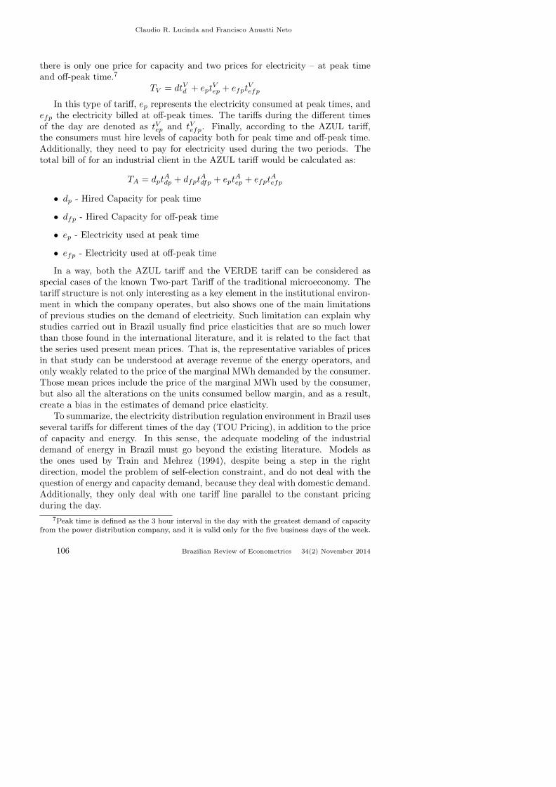
there is only one price for capacity and two prices for electricity – at peak timeand off-peak time.7

TV = dtVd + eptVep + efpt

Vefp

In this type of tariff, ep represents the electricity consumed at peak times, andefp the electricity billed at off-peak times. The tariffs during the different timesof the day are denoted as tVep and tVefp. Finally, according to the AZUL tariff,the consumers must hire levels of capacity both for peak time and off-peak time.Additionally, they need to pay for electricity used during the two periods. Thetotal bill of for an industrial client in the AZUL tariff would be calculated as:

TA = dptAdp + dfpt

Adfp + ept

Aep + efpt

Aefp

• dp - Hired Capacity for peak time

• dfp - Hired Capacity for off-peak time

• ep - Electricity used at peak time

• efp - Electricity used at off-peak time

In a way, both the AZUL tariff and the VERDE tariff can be considered asspecial cases of the known Two-part Tariff of the traditional microeconomy. Thetariff structure is not only interesting as a key element in the institutional environ-ment in which the company operates, but also shows one of the main limitationsof previous studies on the demand of electricity. Such limitation can explain whystudies carried out in Brazil usually find price elasticities that are so much lowerthan those found in the international literature, and it is related to the fact thatthe series used present mean prices. That is, the representative variables of pricesin that study can be understood at average revenue of the energy operators, andonly weakly related to the price of the marginal MWh demanded by the consumer.Those mean prices include the price of the marginal MWh used by the consumer,but also all the alterations on the units consumed bellow margin, and as a result,create a bias in the estimates of demand price elasticity.

To summarize, the electricity distribution regulation environment in Brazil usesseveral tariffs for different times of the day (TOU Pricing), in addition to the priceof capacity and energy. In this sense, the adequate modeling of the industrialdemand of energy in Brazil must go beyond the existing literature. Models asthe ones used by Train and Mehrez (1994), despite being a step in the rightdirection, model the problem of self-election constraint, and do not deal with thequestion of energy and capacity demand, because they deal with domestic demand.Additionally, they only deal with one tariff line parallel to the constant pricingduring the day.

7Peak time is defined as the 3 hour interval in the day with the greatest demand of capacityfrom the power distribution company, and it is valid only for the five business days of the week.



To deal with these problems, the present paper uses a database from companies,with prices they actually face, to estimate the demand elasticity of prices of thedifferent tariff components. The next section describes the methodology used.

3. Empirical Analysis

In this article we propose a structural model to model the industrial demandfor electricity that goes beyond those described above, and is able to integrate thechoice of tariff modality with energy demand in the two periods of the day (peakand off-peak). We assume that the company uses the different types of energy andcapacity mentioned before, thus the function can be described as:

Q = F (ep, efp, dp, dfp,Z) (1)

where Q is the amount produced and Z amounts of other insumes, and the othervariables previsously defined. Assuming the weak separability and homotheticityin the production function we can rewrite this function as:

Q = F (EE(dp, dfp, ep, efp),Z) (2)

where EE is the agregated measure of energy. Given these hypothesis, we candescribe the global cost function, in which CEE is a measure of the Eletric Powercosts, as:

CT = C (CEE (tep, tefp, tdp, tdfp, Q) , PZ, Q) (3)

As a premise of homotheticity and weak separability, we have that the selectioncan be modeled in two steps, the first is choosing a tariff from the menu, and thesecond is determining the different demands for energy and capacity of the differentproducts. Especially, CEE = CA, se CA < CV CA if and CA < CC , where CA isthe cost of an amount EE of energy in the AZUL tariff, is the cost of the sameamount in VERDE tariff, and CC is the cost in the conventional tariff. Similarly,CEE = CV if the cost in the VERDE tariff is lower than in other tariffs.

In this paper we assume a functional form for the cost function in the PIGLOGform:

lnCEE(tep, tefp, tdp, tdfp, Q) = α0+∑k

αk ln tk+1

2

∑j

∑k

γjk ln tj ln tk+Qβ0

∏k

tβk

k

(4)When we carry out the logarithmic differentiation for each of the prices of the

different types of energy, we have the following equations for each of the tariffs:8

sk = αk +∑j

γjk ln tj + βkQβ0

∏k

tβk

k (5)

8Greene (1984) carries out similar modeling for the case of diesel fuel oil demand.



where the variables sk represent the participation in the total expenditure of thek-th type of service. We can write that as CEE = RT − PZZ, that is, the cost ofenergy is the same as the difference between the total revenue minus the expendi-tures with other insumes and economic profits. Assuming that PZZ is a functionof CEE , we can rewrite the equation as:

sk = αk +∑j

γjk ln tj + βk ln

(CEEP

)(6)

where CEE is the total expenditure with energy, as previsously defined and P is anenergy price index, which in this paper assumes a linear form of the Stone Index:

ln P =∑k

sk ln tk

The coefficient βk in the equation above measures the sensitivity of the differentparticipations in the expenditure of the total volume spent with energy. This isa version of the Almost Ideal Demand System of Lee et al. (1980), often used formodeling the demand of homogenous products. Despite being interesting, thismodeling presents additional difficulties for estimations, since the choice betweentariffs and the type of energy consumed are inter-connected. The equations of thesystem components above will be different for each type of tariff chosen (AZUL,VERDE or Conventional). If we ignore this possibility, we might obtain biasedcoefficients, which would represent both the substitution in the use of energybetween the different times of the day and the same modality with substitutionsbetween the different tariff lines. A similar approach is used by Lee, Maddalaand Trost (1980), and which can be applied here, is the characterization of thiseconometric problem as an application of the switching simultaneous equations. Inthis methodology we would have a model with two states. The first is the selectionof tariff modality, and the second the services of that tariff modality. That is, ifthe tariff chosen was the AZUL, the demand for the four services would be:

sep = αep +∑j γj,ep ln tj + βep ln

(CEE

P

)sefp = αefp +

∑j γj,efp ln tj + βefp ln

(CEE

P

)sdp = αdp +

∑j γj,dp ln tj + βdp ln

(CEE

P

)sdfp = αdfp +

∑j γj,dfp ln tj + βdfp ln

(CEE

P

)(7)

In the same manner, if the chosen tariff is the VERDE, we have:

sep = αep +∑j γj,ep ln tj + βep ln

(CEE

P

)sefp = αefp +

∑j γj,efp ln tj + βefp ln

(CEE

P

)sdp = αdp +

∑j γj,dp ln tj + βdp ln

(CEE

P

)(8)



To deal with this problem, we propose the addiction of a selectivity term inthe equations estimated for each of the regimes. This term of selectivity dependson how the tariff choice is specified – since it is a discreet choice model. In thispaper specifically, we have chosen to model the choice of tariff as a multinomialLOGIT, similarly to Dubin and McFadden (1984). With this modeling, a genericequation of the equation system above would be as follows – in the next examplethe tariff chosen is the AZUL:

E(sk|M = A) = αk +∑j

γjk ln tj + βk ln

(CEEP

)(9)

+ σ

r1 ln(PA) +∑j=V,C

rjln(Pj)Pj(1− Pj)

where σ represents the standard deviation of erros in the original equation, andrj the coefficients specific to each selectivity component – which are not identifiedseparately from the coefficient rj . Despite the fact that this specification pro-duces estimates that are assintotically consistent, we have a problem associatedwith inference. Especially, in the presence of the term estimated between brack-ets, the estimates are inefficient. To deal with this problem, the standard-errorswere calculated using bootstrapping, with 100 replications and clustering for eachcompany.9

The model for tariff selection, basis for the calculation of probability of choiceand the selectivity correction factor discussed above, is based on the followingutility function for the alternative j = VERDE, AZUL or Conventional:

Uij = Vij + εj (10)

where Vij denotes the deterministic part of the utility for the consumer i broughtabout by choosing the tariff j and the εj the idiosyncratic part.10 The mean utilityfor the choice of the Conventional tariff was normalized in zero11 and the followingparametrization of the term Vj was adopted:

Vij = φj0 + φj1gi + φj2lfpi + φj3lpi + φj4CEEi + φj5 ln Pi + fs + ti (11)

9We have also tested estimates using only the bootstraping, without clustering, and thestandard deviations calculated as usual. The results are available upon request, and were notreported. In general terms, the results of these alternative estimates were better in terms ofsignificance of the coefficients, and the conclusions drawn in this paper would also be valid forthe alternative method.

10Which we assume follows a Gumbel distribution (also known as extreme values distribution).11Because the companies in this paper are all above 300 kV, they could only choose between

V or AZ. The binary selection models were necessary for VERDE-Conventional because somecompanies were not placed in the correct tariff, they increased the capacity but did not changecontracts. Thus, it would not be adequate to explore this choice as a basis, we would need abasis with companies below 300 kV.



where fs are fixed effects of the sector and ti are fixed effects of time. The tariff“Conventional” was established as the base category, and therefore we assumedVij = 0 for this category. The variable lfp is the load factor during the off-peak time and lp is the load factor during peak time. Regardless of the time,the load factor is an index which demonstrates wether the use of energy is beingdone in a rational and economical manner. This index varies from zero to one,and is obtained using the relation between active energy consumed in a specificperiod of time and the total active energy that could be consumed, if the demandmeasured in the period (maximum demand) was used the whole time. Finally, thevariable g represents the ratio between the peak time demand and the off-peaktime demand. Differently from the load factor, which involves both energy andcapacity, this variable is related only to the relative use of capacity in both periods.Those variables are important for the identification of coefficients.

The coefficients φ are indexed according to the alternative (thus the subscriptj), in an attempt to capture part of the non-observable heterogeneity,12 and thestandard errors in this level are calculated as clustering for each company. Thismodel for choosing the tariff modality was estimated using Maximum Likelihood.

The models in the lower level, which correspond to the system equations pre-sented in (9), were estimated using Seemingly Unrelated Regression, with thepossible imposition of homogeneity and symmetry restrictions in the Slutsky ma-trix and fixed effects for each company in the equations in the upper level. Themain reason for choosing to include the individual effects only in the equation ofthe upper level is that, when those effects are present in the AIDS equations theresulting system is no longer invariant to the unit of price, according to Alstonet al. (2001).

The symmetry conditions are given by:

βij = βji

and the homogeneity conditions by:

∑j

βij = 0

If we assume that the agents always spend 100% of the expenses in these fourproducts, we can also recover the coefficients of the equation that was not directly

12Notice that this paper does not attempt a structural interpretation of the estimate coeffi-cients in the tariff selection model, the goal is simply to characterize the probability of differentchoices of tariff to build the posterior of the sample selection term.



estimated – the so called adding-up restriction:∑i

αi = 1∑i

βij = 0∑i

γi = 0

3.1 Data

For this paper we compiled an energy consumption database for each company,in the period of January 2002 to December 2006. This database was built usinginformation from Eletropaulo on industrial consumers belonging to the followingvoltage (voltage) groups in the supply end:

• A2 – From 88 to 138 kV

• A3a – From 30 to 44 kV

• A4 – From 2.3 to 25 kV

• AS – Voltage below 2.3, supplied by the normal distribution network andexceptionally billed in this group.13

These companies have the characteristic of having consumed over 500kW,which puts them in the category special free consumers. This information re-gards the 646 companies in the industrial sector, whose division, according to theCNAE classification up to two digits, is given in Table 2.

We can observe that there is a good dispersion in terms of sectors covered by thecompanies in the sample, with the companies in the Plastic and Rubber sectorshaving greatest participation, with only 13.7% of the sample. Energy intensivesectors such as metallurgy are relatively unimportant in the sample. In terms ofchoice of tariff, Figure 1 shows the distribution of companies throughout time inthe different tariffs.

13Notice however, that there was only one company in this category, as well as in A3a.



Table 2CNAE classification of the companies in the sample

Freq. Part. Cum.Plastic and Rubber 89 13,78 13,78Automotive Vehicles 55 8,51 22,29Food 51 7,89 30,19Basic Metalurgy 51 7,89 38,08Other Chemical Products 50 7,74 45,82Metal Products (except machinery and equipment) 49 7,59 53,41Machinery and Equipment 45 6,97 60,37Textile 34 5,26 65,63Machinery and Electrical equipment 32 4,95 70,59Editing, printing and reproduction 31 4,8 75,39Pharmaceutical 22 3,41 78,79Clothing and Accessories 18 2,79 81,58Non-metalic minerals 15 2,32 83,9Pulp and paper 14 2,17 86,07Other 13 2,01 88,08Electronic and Comunication mat. 13 2,01 90,09Perfumery, soap, detergent 11 1,7 91,8Extrative 9 1,39 93,19Furniture 7 1,08 94,27Office machines and equipment 7 1,08 95,36ComputersShoes and leather 5 0,77 96,13Other transportation equipment 4 0,62 96,75Metal products (excluindo machinery and equipment) 4 0,62 97,37Oil and alchool refining 4 0,62 97,99Hospital Equipment 3 0,46 98,45Electrical machinery and equipment 3 0,46 98,92Tabacco 2 0,31 99,23Machinery and Equipment 2 0,31 99,54Drinks 1 0,15 99,69Wood 1 0,15 99,85Electronic communication material 1 0,15 100Total 646 100Source: prepared by the authors.



Figure 1Energy categories

As we can see in Figure 1, most of the companies – approximately 50% – usesthe AZUL tariff, while approximately 42% uses the VERDE tariff. The rest ofthe observations (pair of company/month) belong to companies that, during theperiod, changed to the tariff Conventional.14 The existence of observations inthe tariff Conventional makes it possible to use this category as the basis in theselection step of the model.

In Table 3 the variables sefp, sep, sdp and sdfp are related to the participationof energy costs in the expenses of a company in a given month (off-peak and peaktime, respectively), and with the acquisition of capacity (off-peak and peak time,respectively). In term of value, the variables vep, vefp, vdp and vdfp are related tothe expenditure with energy and capacity both for off-peak and peak time. Fromthe notation in the last section, we have that CEE = vep + vefp + vdp + vdfp.

From the previous table we can see that, in average, the largest participation inexpenditure is energy at off-peak time (sefp), corresponding to, in average, 51% ofthe expenditure, while the expenditure with capacity comes in second, but neithertype of expenditure with capacity represents more than 20% of expenditure. Interms of prices, the values are much greater for consumption than capacity.

14From the total of 38,512 initial observations, we have 233 observations regarding the changeof tariff. Of these 233, the most common change was from AZUL tariff to VERDE tariff, with 158observations, and 34 observations from Conventional to VERDE and 21 Conventional to AZUL.Only 16 changed from VERDE to AZUL and the remaining cases changed to the Conventionaltariff. In terms of companies, it means 208 out of the 646. Only in 22 cases do we have morethan one change for the same company. There seems to be no defined temporal standard fortariff switch.



Table 3Descriptive statistics

N Mean Maximum Minimum Standarddeviation

svep 38331,000 0,137 1,000 0,000 0,129svefp 38331,000 0,508 1,000 0,000 0,147svdp 38331,000 0,166 0,786 0,000 0,184svdfp 38331,000 0,190 1,000 0,000 0,123vep 38510,000 12573,659 3,47e+05 0,000 19521,663vefp 38510,000 57178,121 2,70e+06 0,000 1,19e+05vdp 38510,000 26963,723 9,53e+05 0,000 60657,893vdfp 38510,000 12197,661 2,34e+05 0,000 13749,684tdp 38510,000 18,290 34,534 7,470 9,511tdfp 38510,000 8,975 34,347 3,093 3,124tep 38510,000 445,482 910,143 72,099 312,854tefp 38510,000 106,429 182,343 50,779 29,953g 38508,000 0,727 3,500 0,000 0,281lp 38425,000 0,661 2,046 0,000 0,233lfp 38508,000 0,504 1,745 0,002 0,183P 38510,000 4,007 4,538 3,234 0,221CEE 38331,000 10,865 15,203 5,069 1,251

Before we go on to the results of the empirical model, we must make some con-siderations in regards to the identification strategies used. Firstly, it is importantto keep in mind that it is a microdata database for company, and there are nofirst-degree discriminations, that is to say, all the companies face the same pricesin a same tariff. In this sense, there is no endogeneity between the prices chargedto a company and the amount of service consumed by said company. Additionally,these prices are determined within a regulatory tariff review processes, in advance,and based on criteria from the price regulating agency. That is, the price here isnot determined by the intersection between the curve of marginal revenue and thecurve of marginal cost, but based on decisions from ANEEL.

Finally, the question of omitted demand characteristics of the company in themodel of demand for service, inside a tariff, is solved with the tariff selectionmodel. In this modality of simultaneous-switching equations, the term of selec-tivity correction also considers the effects of the company’s characteristics, usingsectorial dummies. Those characteristics controlled by the dummies are commonfor companies in the same sector and constant in time. That is, a limitation of thepresent paper is that the companies’ specific and unobserved characteristics couldcreate a bias in the results.15 With these considerations, we present the results ofthe model for modality discreet choice.

As we can observe from the table above, the difference between the two columnsis the incorporation of dummy variables of time and sector, which elevates thePseudo-R2 to approximately 50%. We can observe that in both cases, an increasein the average price of energy, measured by the index P, reduces the willingness

15The absence of additional information about the companies precluded the use of more robustmethods to control the effects of these on the estimates.



Table 4Model – Modality

Model 1 Model 2

g -2,285 *** -1,366(-14,968) (-1,940)

lp -0,622 ** -1,055(-2,902) (-0,872)

lfp -0,953 ** -1,433(-2,695) (-0,735)

P -7,080 *** -82,770 ***(-37,766) (-24,619)

CEE 3,096 *** 2,476 ***(69,346) (12,107)

Constante 1,408 293,140 ***(1,770) (15,709)

Mod. VERDEg -2,909 *** -1,969 **

(-19,959) (-2,803)lp -3,788 *** -4,679 ***

(-18,455) (-3,874)lfp 0,396 0,414

(1,151) (0,212)P -3,670 *** -75,763 ***

(-20,601) (-22,588)CEE 2,223 *** 1,663 ***

(54,333) (8,165)Constante -0,966 277,708 ***

(-1,260) (14,898)Dummies de Tempo Nao SimDummies de Setor Nao SimNumero de Obs. 38246 38246Pseudo R2 0,363 0,500Qui-Quadrado. 25233,632 34792,983P -Val. Qui2 0,000 0,000Note: asymptotic statistics t between parentheses.

Caption: P -value< 0.01∗∗∗, P -value< 0.05∗∗ and P -value< 0.1∗.



of choosing either tariff, in relation to the basis of the Conventional tariff. Addi-tionally, the greater the expenditure with energy, the greater the incentive for theconsumer to go from the Conventional tariff to either AZUL or VERDE. In termsof implications on the behavior of the consumer, the model with sector and timedummies shows results that are apparently more plausible. In the table below, wehave the elasticities crossed between tariffs VERDE and AZUL in both models.

Table 5Elasticities – Upper level

N Median Minimum Maximum Standarddeviation

Elast Azul-Verde (1) 38246 0,020 0,000 0,055 0,010Elast Verde-Azul (1) 38246 0,010 0,000 0,028 0,005Elast Azul-Verde (2) 38246 0,222 0,000 0,604 0,133Elast Verde-Azul (2) 38246 0,203 0,000 0,553 0,121

Table 5 shows a greater substitution between tariffs in the case with the sectorand time dummies, with a mean elasticity between companies of 0.2 – that is, witha 1% increase in P, there is a change among between tariffs of 0.2%. In the modelswithout fixed effects of time and sector, this substitution is of 0.02, implicatingthat there is no substitution between tariffs, which doesn’t seem plausible. Inregards to the specific models for the AZUL and VERDE tariffs, the results areas follows: In each table we observe four columns, two associated to with eachone of the discreet choice models, with and without the time and sector dummies– with selection values that are specific for each model. In each pair of columnswe have the model being estimated with and without symmetry and homogeneityrestrictions.16

From the results in the table above we can observe that the selection terms ofthe different equations are significant in all of them, indicating that if we ignorethe effects of prices on the probability of tariff switch we could cause a significantbias in the price sensitivity of the relevant energy demand margins. From thoseestimates, it is possible to calculate the elasticity for each type of service on eachtariff:

From the results, we can draw some important conclusions on the character-istics of industrial demand for energy, Firstly, we have that for all services thedemand is greatly elastic for price, indicating that the response of the amount ofservice demanded (energy or capacity) to an increase of 1% in the price of theservice is much greater than 1%. Additionally, the pattern of crossed elasticity issuch that there is substitution during the day, that is, in response to an increasein price only during one part of the day, consumers shift their demand for the timeof the day in which the price did not increase. Another interesting point is the

16The third restriction, the adding-up, is used to recover the coefficients of the equation thatwas not estimated.



Table 6AZUL tariff model

Without R.(a) With R. (b) Without R. (c) With R. (d)

Eq. (sep)ln(tDP ) -0,058*** -0,034*** -0,021 -0,057***

(-4,519) (-6,577) (-1,558) (-10,461)ln(tDFP ) 0,088*** 0,040*** 0,075*** 0,057***

(12,930) (12,301) (10,460) (15,925)ln(tEP ) -0,089*** -0,014*** -0,096*** -0,032***

(-19,254) (-3,344) (-20,989) (-7,486)ln(tEFP ) 0,111*** 0,008 0,101*** 0,033***

(17,988) (1,821) (16,187) (7,062)ln(CEE/P) -0,015*** -0,004*** -0,014*** -0,009***

(-18,355) (-4,526) (-22,964) (-14,726)ln(PA)-Mod.1 0,035*** 0,035***

(40,700) (40,225)ln(PC )PC/(1 − PC )-Mod.1 -0,080*** -0,148***

(-13,505) (-25,844)ln(PV )PV /(1 − PV )-Mod.1 0,089*** 0,021***

(25,027) (7,287)ln(PA)-Mod.2 0,019*** 0,018***

(24,585) (23,245)ln(PC )PC/(1 − PC )-Mod.2 -0,087*** -0,110***

(-4,941) (-6,279)ln(PV )PV /(1 − PV )-Mod.2 0,089*** 0,043***

(32,730) (18,599)Constant 0,223*** 0,197*** 0,199*** 0,270***

(16,837) (20,532) (14,844) (31,272)Eq. (sefp)

ln(tDP ) -0,109*** 0,198*** -0,174*** 0,176***(-3,685) (24,687) (-5,584) (20,958)

ln(tDFP ) 0,105*** -0,138*** 0,144*** -0,142***(6,696) (-28,535) (8,704) (-27,244)

ln(tEP ) -0,260*** 0,008 -0,254*** 0,033***(-24,269) (1,821) (-24,032) (7,062)

ln(tEFP ) 0,289*** -0,069*** 0,317*** -0,067***(20,228) (-10,381) (22,147) (-9,921)

ln(CEE/P) 0,056*** 0,078*** 0,052*** 0,065***(28,906) (45,214) (36,143) (47,716)

ln(PA)-Mod.1 -0,040*** -0,043***(-19,968) (-21,371)

ln(PC )PC/(1 − PC )-Mod.1 0,167*** 0,056***(12,132) (4,291)

ln(PV )PV /(1 − PV )-Mod.1 -0,099*** -0,191***(-12,034) (-28,953)

ln(PA)-Mod.2 -0,018*** -0,023***(-10,373) (-13,514)

ln(PC )PC/(1 − PC )-Mod.2 0,290*** 0,103*(7,108) (2,556)

ln(PV )PV /(1 − PV )-Mod.2 -0,056*** -0,130***(-8,922) (-25,027)

Constant 0,149*** -0,348*** 0,180*** -0,265***(4,854) (-20,875) (5,827) (-18,863)

Eq. (sdp)

ln(tDP ) 0,234*** -0,326*** 0,329*** -0,251***(7,791) (-25,700) (10,186) (-18,365)

ln(tDFP ) -0,206*** 0,162*** -0,261*** 0,132***(-12,918) (21,776) (-15,233) (15,916)

ln(tEP ) 0,245*** -0,034*** 0,229*** -0,057***(22,476) (-6,577) (20,875) (-10,461)

ln(tEFP ) -0,239*** 0,198*** -0,270*** 0,176***(-16,497) (24,687) (-18,171) (20,958)

ln(CEE/P) -0,031*** -0,051*** -0,029*** -0,041***(-15,955) (-28,720) (-19,787) (-28,953)

ln(PA)-Mod.1 0,050*** 0,053***(24,637) (26,055)

ln(PC )PC/(1 − PC )-Mod.1 -0,286*** -0,195***(-20,477) (-14,512)

ln(PV )PV /(1 − PV )-Mod.1 0,118*** 0,186***(14,077) (26,871)

ln(PA)-Mod.2 0,016*** 0,020***(8,703) (11,322)

ln(PC )PC/(1 − PC )-Mod.2 -0,419*** -0,169***(-9,922) (-4,028)

ln(PV )PV /(1 − PV )-Mod.2 0,072*** 0,125***(11,107) (22,388)

Constant 0,109*** 0,835*** 0,088** 0,755***(3,483) (47,046) (2,758) (49,031)

Number of Obs. 19042 19042 19039 19039R-sq 1st eq. 0,181 0,143 0,144 0,106R-sq 2nd eq. 0,246 0,214 0,220 0,177R-sq 3rd eq. 0,132 0,088 0,070 0,020

Note: asymptotic statistics t between parentheses. Caption: P -value< 0.01∗∗∗, P -value< 0.05∗∗,and P -value< 0.1∗.



Table 7VERDE tariff model

Without R. (e) With R. (f) Without Restr. (g) With Restr. (h)

Eq. (sep)ln(tDFP ) -0,303*** -0,080 0,095 0,114**

(-4,775) (-1,923) (1,405) (2,616)ln(tEP ) 0,504*** 0,131** -0,069 -0,071

(7,243) (3,000) (-0,930) (-1,561)ln(tEFP ) -0,068*** -0,051*** -0,042*** -0,043***

(-12,033) (-9,733) (-7,406) (-8,756)ln(CEE/P) -0,046*** -0,038*** -0,031*** -0,031***

(-15,875) (-13,624) (-17,993) (-18,009)ln(PV )-Mod.1 0,030*** 0,034***

(9,156) (10,450)ln(PC )PC/(1 − PC )-Mod.1 -0,236*** -0,262***

(-19,283) (-21,953)ln(PA)PA/(1 − PA)-Mod.1 -0,571*** -0,555***

(-62,224) (-61,347)ln(PV )-Mod.2 -0,034*** -0,034***

(-13,348) (-13,645)ln(PA)PA/(1 − PA)-Mod.2 -0,352*** -0,351***

(-49,538) (-49,640)ln(PC )PC/(1 − PC )-Mod.2 -0,320*** -0,326***

(-5,183) (-5,329)Constante -2,176*** -0,296 0,662* 0,643**

(-6,902) (-1,543) (1,983) (3,213)Eq. (sefp)

ln(tDFP ) 0,118* -0,119*** -0,092 -0,121***(1,985) (-13,061) (-1,482) (-13,029)

ln(tEP ) -0,408*** -0,051*** -0,061 -0,043***(-6,252) (-9,733) (-0,895) (-8,756)

ln(tEFP ) 0,185*** 0,169*** 0,204*** 0,204***(35,065) (36,702) (38,995) (48,187)

ln(CEE/P) 0,131*** 0,125*** 0,085*** 0,085***(48,265) (47,236) (53,471) (53,486)

ln(PV )-Mod.1 0,005 0,002(1,627) (0,619)

ln(PC )PC/(1 − PC )-Mod.1 -0,032** -0,012(-2,772) (-1,090)

ln(PA)PA/(1 − PA)-Mod.1 0,402*** 0,389***(46,646) (45,601)

ln(PV )-Mod.2 0,024*** 0,024***(10,194) (10,379)

ln(PA)PA/(1 − PA)-Mod.2 0,220*** 0,220***(33,519) (33,616)

ln(PC )PC/(1 − PC )-Mod.2 0,008 0,015(0,135) (0,257)

Constante 1,527*** -0,230*** -0,198 -0,257***(5,163) (-8,445) (-0,642) (-11,306)

Numero de Obs. 16228 16228 16228 16228R-sq 1a eq. 0,356 0,352 0,299 0,299R-sq 2a eq. 0,355 0,352 0,315 0,315

Note: asymptotic statistics t between parentheses. Caption: P -value< 0.01∗∗∗, P -value< 0.05∗∗,and P -value< 0.1∗.



Table 8Elasticities – AZUL Tariff

Model (a) Model (b)tep tefp tdp tdfp tep tefp tdp tdfp

ep -1,636*** 0,869*** -0,404*** 0,662*** -1,099*** 0,073** -0,246*** 0,298***(0,034) (0,046) (0,094) (0,050) (0,031) (0,034) (0,038) (0,024)

efp -0,527*** -0,487*** -0,233*** 0,186*** -0,005* -1,213*** 0,364*** -0,300***

(0,021) (0,029) (0,058) (0,031) (0,009) (0,014) (0,016) (0,010)dp 1,500*** -1,347*** 0,443** -1,205*** -0,164*** 1,349*** -2,912*** 1,034***

(0,065) (0,009) (0,181) (0,096) (0,031) (0,051) (0,076) (0,045)dfp 0,556*** -0,820*** -0,348*** -0,920*** 0,229*** -0,661*** 0,875*** -1,316***

(0,024) (0,034) (0,068) (0,036) (0,017) (0,026) (0,039) (0,024)

Model (c) Model (d)tep tefp tdp tdfp tep tefp tdp tdfp

ep -1,692*** 0,790*** -0,137* 0,571*** -1,227*** 0,274*** -0,409*** 0,428***(0,033) (0,046) (0,099) (0,053) (0,031) (0,035) (0,040) (0,026)

efp -0,515*** -0,426*** -0,360*** 0,265*** 0,047*** -1,197*** 0,326*** -0,304***

(0,021) (0,029) (0,062) (0,033) (0,009) (0,014) (0,016) (0,010)dp 1,402*** -1,535*** 1,014*** -1,541*** -0,312*** 1,189*** -2,471*** 0,840***

(0,066) (0,091) (0,195) (0,103) (0,033) (0,052) (0,082) (0,050)dfp 0,650*** -0,762*** -0,698*** -0,772*** 0,310*** -0,709*** 0,708*** -1,229***

(0,026) (0,036) (0,077) (0,041) (0,019) (0,028) (0,044) (0,028)

Note: Standard Deviations calculated using the Delta Method.Caption: P -value< 0.01∗∗∗. P -value< 0.05∗∗, and P -value< 0.1∗.

result that this shift of demand is even more intense from peak time to off-peaktime than the inverse.

Finally, the negative crossed elasticities between energy and capacity are in-dicative of complementarity between both products – that is, an increase in theprice of energy in the off-peak time reduces the demand for energy at that time inaddition to reducing the capacity.

In Table 9 we have the calculation of the price and crossed elasticity for thecompanies in the VERDE tariff.

Table 9Elasticities – VERDE Tariff

Model (e) Model (f)tep tefp td tep tefp td

ep 2,735*** -0,323*** -2,154*** -0,005 -0,232*** -0,533(0,509) (0,046) (0,465) (0,319) (0,044) (0,305)

efp -0,839*** -0,768*** 0,184* -0,134*** -0,793*** -0,281***(0,129) (0,012) (0,117) (0,010) (0,011) (0,018)

d -0,444* -0,389*** 0,060* -0,359 -0,388*** 0,137(0,233) (0,021) (0,212) (0,219) (0,021) (0,204)

Model (g) Model (h)tep tefp td tep tefp td

ep -1,471*** -0,191*** 0,735 -1,493*** -0,200*** 0,880***(0,540) (0,043) (0,493) (0,335) (0,037) (0,320)

efp -0,143 -0,684*** -0,213 -0,107*** -0,684*** -0,270***(0,135) (0,011) (0,123) (0,010) (0,009) (0,018)

d 0,723*** -0,709*** -0,958*** 0,642*** -0,703*** -0,910***(0,244) (0,019) (0,222) (0,231) (0,019) (0,214)

Note: Standard Deviations calculated using the Delta Method.

Caption: P -value< 0.01∗∗∗, P -value< 0.05∗∗, and P -value< 0.1∗.

The results here indicate that the energy demand on peak time is elastic, whilethe energy demand on off-peak time and the demand for capacity are inelastic.



Regarding the substitution and complementarity pattern, only energy at peaktime and capacity are substituted, while energy at off-peak time and capacityare complementary. That is, an increase in the price of off-peak energy causes areduction of peak time energy and of hired capacity as well.

These results seem different from those obtained for the AZUL tariff, but it isimportant to keep in mind the role of hired capacity in this case. A unit of capacityused during peak time means that there is one less unit of capacity available forthe off-peak time and vice-versa. In this sense, we can interpret the response tothe increase in prices of off-peak energy as follows: in response to the increasein tariff, the company reduces its aggregated energy consumption. However, thisreduction is asymmetric during the day, and the off-peak consumption is smallerand to absorb part of this shift the company acquires more units of capacity.

We can also draw some conclusions from the comparison of results for theVERDE and AZUL tariffs as presented in Table (1). Firstly, as expected, thedifferent demands here represented are a lot more elastic than what was presentedfor the aggregated energy demand in the introduction. That is, the price sensitivityof the different components of industrial energy demand is much greater than thatof the aggregated demand, in addition to the fact that the estimates mentioned inTable (1) could be biased due to the use of the average price as an approximationof the perceived cost of the marginal energy consumption.

Another dimension in which it is possible to argue that the results here pre-sented constitute and advance in relation to the existing literature is the fact that,in this study, we estimate the crossed sensitivity between the different types ofenergy and capacity, making it possible to draw an analysis not only on the abso-lute level of tariffs, but also on how the tariff load is spread among the differentservices (energy and capacity at peak time and off-peak time). From the resultsof the elasticities previously discussed, we can carry out a simulation exercise onthe tariff changes proposed from the 2012 and 2013, referring to the relative pricebetween the different service tariffs. In the next table, we show the results com-puted from the elasticities of the models (d) , for the AZUL tariff, and (h) for theVERDE tariff.

Table 10Tariff changes and effect on quantities

AZUL VERDEType Price Amount Type Price Amount

variation variation variation variationep -9,10% 8,06% ep -9,10% -37,97%efp -9,30% 10,05% efp -9,30% 23,72%dp -29,60% 40,06% d -60,70% 55,93%dfp -29,60% 19,19%

This table shows us that, with the proposed reduction in prices of services –and keeping the disposition to maintain the same type of tariffs – would cause a



shift in the consumption of energy, from peak time to off-peak time. In the caseof the VERDE tariff, the movement is stronger, with a reduction of peak energyand an increase in off-peak energy. In the case of the AZUL tariff, is that thepeak energy increases more than the off-peak. And all those changes would beeven stronger than we could have predicted had we used the estimates of priceelasticity of the industrial energy demand in Table (1).

4. Conclusions

In this paper we proposed an econometric model for the demand of energyand capacity by Brazilian industrial consumers. Differently from the residentialconsumers, the Brazilian industrial consumers, besides consuming energy and ca-pacity, also face a tariff menu with Time of Use Pricing. Additionally, each ofthe three tariffs (AZUL, VERDE or Conventional) also has different componentsand price discriminations. All these characteristics combined pose an empiricalproblem, which, up to this moment, had not been faced by the literature.

Because the choice of those tariffs is not mandatory – the consumers can pickwhich one is more suitable to them – the estimate of energy and capacity demandin each of the tariffs without taking into account the problem of tariff selectioncould lead to a bias in the estimated coefficients of the demand function. To dealwith this problem we, initially estimated a multinomial discreet selection model,and later used the selection probabilities in a way to assure that the coefficientestimates were not biased.

This methodology was applied to a non-random sample of 646 large Brazilianindustrial consumers (with demand above 300 KW), for the period from January2002 to December 2006. We observed that the demands for different services (peakand off-peak capacity and energy) are price elastic and that, at least in the AZULtariff, there is complementarity between energy and capacity in the different timesof the day.

Additionally, the conclusions on tariff structure are based on estimates of ag-gregated electricity demand price elasticity, with disaggregation of consumption atdifferent times of the day, which could lead to incorrect policy conclusions. The in-dustrial energy price elasticity estimates in the Brazilian literature evaluate mostlythe average consumption of energy. However, the price system used by the Agencyrecognizes the importance of distinguishing the use of energy and capacity (kW),with the later determining the dimensioning of the distribution system, and con-sequently of investments. Thus, it is important to know the degree of substitutionbetween energy and power in both periods, and this is an original contribution inthis paper. The importance of this information was highlighted with a simulationexercise carried out in the end of the paper, in which we evaluate a propositionthat, besides a reduction in prices, we would have also a change in the relativeprices of energy and capacity. The obtained effects were much more importantthan what we would have obtained using the simple application of results found



in the literature.

References

Aigner, D. (1985). The residential electricity time-of-use pricing experiments:What have we learned? In Social Experimentation, NBER Chapters, pages11–54. National Bureau of Economic Research, Inc.

Aigner, D. J. & Hirschberg, J. G. (1985). Commercial/industrial customer responseto time-of-use electricity prices: Some experimental results. The RAND Journalof Economics, 16(3):341–355.

Alston, J. M., Chalfant, J. A., & Piggott, N. E. (2001). Incorporating demandshifters in the almost ideal demand system. Economics Letters, 70(1):73–78.

Andrade, T. A. & Lobao, W. J. A. (1997). Elasticidade renda e preco da demandaresidencial de energia eletrica no Brasil. Texto para Discussao No 489.

ANEEL (2009). Proposta de alteracao metodologica da estrutura tarifaria apli-cada ao setor de distribuicao de energia eletrica no Brasil, 1a. parte. Technicalreport, ANEEL, Brasilia. Nota Tecnica n◦ 271/2009-SRE-SRD/ANEEL, de04/08/2009.

Bjorner, T. B., Togeby, M., & Jensen, H. H. (2001). Industrial companies’ demandfor electricity: Evidence from a micropanel. Energy Economics, 23(5):595–617.

Bohi, D. R. & Zimmerman, M. B. (1984). An update on econometric studies ofenergy demand behavior. Annual Review of Energy, 9:105–54.

Borenstein, S. & Holland, S. (2005). On the efficiency of competitive electricitymarkets with time-invariant retail prices. RAND Journal of Economics, pages469–493.

de Mattos, L. B. (2005). Uma estimativa da demanda industrial de energia eletricano Brasil: 1974-2002. Organizacoes Rurais e Agroindustriais, 7(2):238–246.

de Mattos, L. B. & de Lima, J. E. (2005). Demanda residencial de energia eletricaem Minas Gerais: 1970-2002 [residential demand for electrical energy in MinasGerais: 1970-2002]. Nova Economia, 15(3):31–52.

Dubin, J. A. & McFadden, D. L. (1984). An econometric analysis of residentialelectric appliance holdings and consumption. Econometrica, 52(2):345–62.

Faruqui, A. & Malko, J. R. (1983). The residential demand for electricity bytime-of-use: A survey of twelve experiments with peak load pricing. Energy,8(10):781–795.



Faruqui, A. & Sergici, S. (2010). Household response to dynamic pricing of electric-ity: A survey of 15 experiments. Journal of Regulatory Economics, 38:193–225.

Filippini, M. (1995). Electricity demand by time of use an application of thehousehold aids model. Energy Economics, 17(3):197–204.

Greene, D. L. (1984). A derived demand model of regional highway diesel fuel use.Transportation Research Part B: Methodological, 18(1):43–61.

Griffin, J. M. (1993). Methodological advances in energy modelling: 1970-1990.The Energy Journal, 14(1):111–124.

Irffi, G., Castelar, I., Siqueira, M. L., & Linhares, F. C. (2009). Previsao dademanda por energia eletrica para classes de consumo na regiao nordeste, usandoOLS dinamico e mudanca de regime. Economia Aplicada, 13(1):69–98.

Lee, L.-F., Maddala, G. S., & Trost, R. P. (1980). Asymptotic covariance matricesof two-stage probit and two-stage Tobit methods for simultaneous equationsmodels with selectivity. Econometrica, 48(2):491–503.

MME/EPE (2012). Plano decenal de expansao de energia, 2021. Technical report,Ministerio das Minas e Energia, Empresa de Pesquisa Energetica.

Modiano, E. M. (1984). Elasticidade-renda e precos da demanda de energia eletricano Brasil. Texto para Discussao no 68 – Departamento de Economia PUC-RIO.

Schmidt, C. A. J. & Lima, M. A. M. (2004). A demanda por energia eletrica noBrasil. Revista Brasileira de Economia, 58(1):67–98.

Sheen, J.-N., Chen, C.-S., & Wang, T.-Y. (1995). Response of large industrialcustomers to electricity pricing by voluntary time-of-use in Taiwan. Generation,Transmission and Distribution, IEE Proceedings-, 142(2):157–166.

Siqueira, M. L., de Hollanda Cordeiro Junior, H., & Castelar, I. (2006). A demandapor energia eletrica no nordeste brasileiro apos o racionamento de 2001-2002:Previsoes de longo prazo. Pesquisa e Planejamento Economico, 36(1):137–178.

Taylor, L. D. (1975). The demand for electricity: A survey. Bell Journal ofEconomics, 6(1):74–110.

Train, K. & Mehrez, G. (1994). Optional time-of-use prices for electricity: Econo-metric analysis of surplus and pareto impacts. The RAND Journal of Economics,25(2):263–283.


Non-linear Demand and Price: An Empirical Analysis of the Brazilian Industrial Electricity...

Documents

Transcript of Non-linear Demand and Price: An Empirical Analysis of the Brazilian Industrial Electricity...