Dynamical study and robustness for a nonlinear wastewater treatment model
14
Nonlinear Analysis: Real World Applications 12 (2011) 487–500 Contents lists available at ScienceDirect Nonlinear Analysis: Real World Applications journal homepage: www.elsevier.com/locate/nonrwa Dynamical study and robustness for a nonlinear wastewater treatment model M. Serhani a,∗ , J.L. Gouze b , N. Raissi c a Equipe TSI, Mathematics and Computer Department, Faculty of Sciences, University Moulay Ismail, BP 11201, Zitoune, Meknes, Morocco b Projet COMORE, INRIA-Sophia Antipolis, B.P. 93, France c EIMA, Mathematics and Computer Department, Faculty of Sciences, University Ibn Tofail, B.P. 133, Kenitra, Morocco article info Article history: Received 4 June 2010 Accepted 27 June 2010 This paper is dedicated to Serhani Khadija. Keywords: Dynamical system Asymptotical stability Lyapunov function Robustness Wastewater treatment abstract In this work we deal with a wastewater treatment by using the activated sludge process. The problem is formulated as a nonlinear dynamical system. Firstly, we develop the dynamical study of the model when all parameters are well known. Hence, basic properties of invariance and dissipation are established and, under a suitable condition on parameters, a globally asymptotically stable equilibrium point occurs. Secondly, when the bacterium growth function and the substrate concentration in the feed stream are not well known, the robustness analysis provides the existence of an attractor domain to which all trajectories of the system converge. Finally, we prove that we can reduce the size (volume) of this attractor domain by increasing the recycle rate to a maximum fixed level. © 2010 Elsevier Ltd. All rights reserved. 1. Introduction In this paper, we study a problem of wastewater treatment, namely that of the activated sludge process in a depura- tion station. The mathematical model is formulated as a nonlinear ordinary differential system. The working principle is described thoroughly in the literature (see for example [1–6]). Basically, the process can be summarized as follows: the wastewater is discharged into an aerator with a flow Q in and a concentration s in in the feed stream. The phase of biological oxidation of the polluted water (substrate), by a blend of a bacterial population in an aerobic reaction consuming the oxy- gen, begins in the aerator and completes in the settler tank. At this stage, due to gravity, the solid components will settle and concentrate at the bottom, while the sedimentation of soluble organic matter is assumed to be not significant. Part of the bacteria biomass is recycled into the aerator in order to stimulate the oxidation. A schematic of the process is shown in Fig. 1, where s, x and x r are the state variables representing respectively the substrate biomass (pollutant), the bacteria biomass and the recycled bacteria biomass concentrations. Q in , Q out , Q r , Q w are the influent, effluent, recycle and waste flow rates, respectively. V a and V s represent the aerator and settler volumes and s in corresponds to the substrate concentrations in the feed stream. Although many works showed interest in a similar problem, where biological aspects and aspects of observability [2–8], estimation, adaptive control, computer simulation [6,9–13], and numerical optimal control [5,14] were studied, there appears to be no work focused upon the dynamical behavior of a model involving a nonlinear bacterium growth function, Our goal in this work is to carry out a rigorous dynamical study for two cases: firstly, when all parameters of the model are known, and secondly, when some parameters are not known. Hence, in the first part of this paper, the basic properties of invariance and dissipation are established and we prove that under some conditions on parameters, there ex- ists a globally asymptotically stable interior equilibrium point. In the second part, our attention is focused on the case where ∗ Corresponding author. E-mail addresses: [email protected] (M. Serhani), [email protected] (J.L. Gouze), [email protected] (N. Raissi). 1468-1218/$ – see front matter © 2010 Elsevier Ltd. All rights reserved. doi:10.1016/j.nonrwa.2010.06.034
Transcript of Dynamical study and robustness for a nonlinear wastewater treatment model
Nonlinear Analysis: Real World Applications 12 (2011) 487–500
Contents lists available at ScienceDirect
Nonlinear Analysis: Real World Applications
journal homepage: www.elsevier.com/locate/nonrwa
Dynamical study and robustness for a nonlinear wastewatertreatment modelM. Serhani a,∗, J.L. Gouze b, N. Raissi ca Equipe TSI, Mathematics and Computer Department, Faculty of Sciences, University Moulay Ismail, BP 11201, Zitoune, Meknes, Moroccob Projet COMORE, INRIA-Sophia Antipolis, B.P. 93, Francec EIMA, Mathematics and Computer Department, Faculty of Sciences, University Ibn Tofail, B.P. 133, Kenitra, Morocco
a r t i c l e i n f o
Article history:Received 4 June 2010Accepted 27 June 2010
This paper is dedicated to Serhani Khadija.
Keywords:Dynamical systemAsymptotical stabilityLyapunov functionRobustnessWastewater treatment
a b s t r a c t
In this work we deal with a wastewater treatment by using the activated sludge process.The problem is formulated as a nonlinear dynamical system. Firstly, we develop thedynamical study of themodelwhen all parameters arewell known. Hence, basic propertiesof invariance and dissipation are established and, under a suitable condition on parameters,a globally asymptotically stable equilibrium point occurs. Secondly, when the bacteriumgrowth function and the substrate concentration in the feed stream are notwell known, therobustness analysis provides the existence of an attractor domain to which all trajectoriesof the system converge. Finally, we prove that we can reduce the size (volume) of thisattractor domain by increasing the recycle rate to a maximum fixed level.
© 2010 Elsevier Ltd. All rights reserved.
1. Introduction
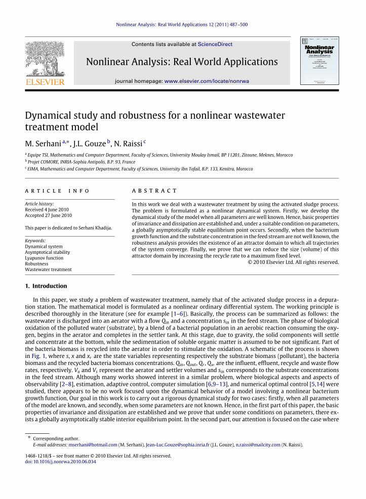
In this paper, we study a problem of wastewater treatment, namely that of the activated sludge process in a depura-tion station. The mathematical model is formulated as a nonlinear ordinary differential system. The working principle isdescribed thoroughly in the literature (see for example [1–6]). Basically, the process can be summarized as follows: thewastewater is discharged into an aerator with a flow Qin and a concentration sin in the feed stream. The phase of biologicaloxidation of the polluted water (substrate), by a blend of a bacterial population in an aerobic reaction consuming the oxy-gen, begins in the aerator and completes in the settler tank. At this stage, due to gravity, the solid components will settleand concentrate at the bottom, while the sedimentation of soluble organic matter is assumed to be not significant. Part ofthe bacteria biomass is recycled into the aerator in order to stimulate the oxidation. A schematic of the process is shownin Fig. 1, where s, x and xr are the state variables representing respectively the substrate biomass (pollutant), the bacteriabiomass and the recycled bacteria biomass concentrations. Qin, Qout, Qr , Qw are the influent, effluent, recycle and waste flowrates, respectively. Va and Vs represent the aerator and settler volumes and sin corresponds to the substrate concentrationsin the feed stream. Although many works showed interest in a similar problem, where biological aspects and aspects ofobservability [2–8], estimation, adaptive control, computer simulation [6,9–13], and numerical optimal control [5,14] werestudied, there appears to be no work focused upon the dynamical behavior of a model involving a nonlinear bacteriumgrowth function, Our goal in this work is to carry out a rigorous dynamical study for two cases: firstly, when all parametersof themodel are known, and secondly, when some parameters are not known. Hence, in the first part of this paper, the basicproperties of invariance and dissipation are established and we prove that under some conditions on parameters, there ex-ists a globally asymptotically stable interior equilibrium point. In the second part, our attention is focused on the case where
∗ Corresponding author.E-mail addresses:[email protected] (M. Serhani), [email protected] (J.L. Gouze), [email protected] (N. Raissi).
1468-1218/$ – see front matter© 2010 Elsevier Ltd. All rights reserved.doi:10.1016/j.nonrwa.2010.06.034
488 M. Serhani et al. / Nonlinear Analysis: Real World Applications 12 (2011) 487–500
Fig. 1. Schematic diagram of the activated sludge process.
the bacterium growth functionµ and the substrate concentration in the feed stream sin are not known, only their upper andlower bounds. Indeed, due to metabolic variations and the influence of many physico-chemical factors (pH, temperature,oxygen, . . . ), it is very hard to obtain full information on the bioprocess kinetics and an accurate idea of µ (see e.g. [3,15]). Inthis framework, a robustness analysis of the model, invoking the monotone and cooperative system theory, leads to the factthat there exists an interior domain of stability U , instead a unique stable equilibrium point. Finally, we propose a simpleway to reduce the size (volume) of the stability domain by increasing the value of the recycle rate r , and hence the stabilitydomain reaches its minimal value when r achieves its maximum level.
2. Mathematical model
In themodel, we assume that the aerator is sufficiently aerated to provide the dissolved oxygen necessary for the growthof the bacterial population; as a consequence the oxygen reaction is neglected. Three phenomena are considered: thereaction kinetics in the aerator linked to microbial growth, the substrate degradation and the recycling of the biomass fromthe settler. The mass balance of the various constituents gives the following set of equations:
(S)
dsdt
= s = −µ(s)xY
− (1 + r)Ds + Dsin; s(0) = s0
dxdt
= x = µ(s)x − (1 + r)Dx + rDxr; x(0) = x0
dxrdt
= xr = ν(1 + r)Dx − ν(w + r)Dxr; xr(0) = xr0
with
D =Qin
Va; r =
Qr
Qin; w =
Qw
Qin; ν =
Va
Vs,
and where Y refers to the yield coefficient of the growth of biomass on the substrate. µ is the specific growth rate functionof the bacterium.
2.1. Hypotheses
We assume thatA1 D, r , w and ν are positive constants.A2 µ : R+
→ R+ is a C2 monotone increasing function and satisfies
0 ≤ µ(.) ≤ mµ(s) = 0 if s = 0
where m is a given constant.
A classical example of the function µ is the so-called Monad function, given by the following formulation:
µ(s) :=ms
k + s,
where k is a given constant.
3. Dynamical analysis
In this section we are interested in the asymptotic behavior of nonnegative solutions of the model (S) under the assump-tions A1 and A2, i.e. when all parameters are fully known.
3.1. Invariance and dissipation
The aim is to establish the basic properties of invariance and dissipation.Consider the open subset of R3
+, Ω := (s, x, xr) ∈ R3
+/s > 0, x > 0, xr > 0,. Firstly, we look for the invariance of Ω .
M. Serhani et al. / Nonlinear Analysis: Real World Applications 12 (2011) 487–500 489
Proposition 1. The set Ω is positively invariant for the system (S).
Proof. On the boundary of Ω , ∂Ω:If x = 0 with xr > 0 and s ≥ 0 then x = rDxr > 0, so the vector field of x is pointed to inside Ω .Likewise if xr = 0 with x > 0 and s ≥ 0 then xr = ν(1 + r)D > 0 and then the flow of xr is pointed to inside Ω .Now if s = 0, with (x ≥ 0 and xr > 0) or (x > 0 and xr ≥ 0) then s = Dsin > 0.To conclude, it remains to show that the line G := (s, x, xr) s.t. s ≥ 0, x = xr = 0 is invariant. But on G the system is
reduced tos = −(1 + r)Ds + Dsinx = 0xr = 0
which shows by standard arguments for linear ODE that s ≥ 0 and hence that G is invariant.
We can now claim that the system (S) is dissipative, that is, all nonnegative trajectories are uniformly bounded in thepositive octant R+.
Proposition 2. All nonnegative solutions of (S) are uniformly bounded in Ω (closure of Ω).
Proof. Let u(t) = (s(t), x(t), xr(t)) in Ω and consider
α(t) :=xr(t)
xr(t) + νx(t).
We have 0 < α < 1.Let us now prove the following result:
Lemma 3. There exist a constant η > 0 sufficiently small and T (η) > 0 such that for all t ≥ T (η) we have η ≤ α(t) ≤ 1 − η.
Proof. By taking the derivative of α, we have
dαdt
= α = νxrx − xr x(xr + νx)2
.
But
xrx − xr x = ν(1 + r)Dx2 − ν(w + r)Dxrx − µ(s)xxr + (1 + r)Dxxr − rDx2r= x(1 + r)D[νx + xr ] − rDxr [xr + νx] − (νwD + µ(s))xxr .
Hence
α = −rDα + ν(1 + r)Dx
xr + νx− ν(νwD + µ(s))
xxr(xr + νx)2
.
Taking into account of the fact that 1 − α =νx
xr+νx , it follows that
α = −rDνα + (1 + r)D(1 − α) − α(1 − α)(νwD + µ(s)).
By choosingM = νwD + m, where m is given by hypothesis A1, we obtain that
α ≤ −rDνα + (1 + r)D(1 − α) + α(1 − α)M
and
α ≥ −rDνα + (1 + r)D(1 − α) − α(1 − α)M.
Consider two functions F+ and F− as
F+(z) = −rDνz + (1 + r)D(1 − z) + z(1 − z)M
and
F−(z) = −rDνz + (1 + r)D(1 − z) − z(1 − z)M.
Observe that F+(1) = −rDν < 0 and F−(0) = (1 + r)D > 0, so, according to the continuity of F− and F+, there existη , δ > 0 such that
∀z, 1 − η ≤ z ≤ 1 H⇒ F+(z) ≤ −δ < 0
and
∀z, 0 ≤ z ≤ η H⇒ F−(z) ≥ δ > 0.
490 M. Serhani et al. / Nonlinear Analysis: Real World Applications 12 (2011) 487–500
On the other hand, we haveα(t) ≤ F+(α(t))α(t) ≥ F−(α(t)).
So,
∀α(t), 1 − η ≤ α(t) ≤ 1 H⇒ α(t) ≤ F+(α(t)) ≤ −δ < 0
and
∀α(t), 0 ≤ α(t) ≤ η H⇒ α(t) ≥ F−(α(t)) ≥ δ > 0
which implies that there exists a T (η) > 0 such that
∀t ≥ T (η) α(t) ∈ [η, 1 − η]
as required.
Return to the proof of the proposition and consider Σ := νx + νYs + xr .We have
Σ = −(1 + r)D[νx + νYds − νx] + rDνxr − ν(w + r)Dxr + DνYsin= −(1 + r)DνYds − νwDxr + DνYsin≤ −kD(xr + νYds) + DνYsin
where k = min(νw, 1 + r).Since ηs ≤ s and according to the previous lemma, the inequality xr ≥ η(xr + νx) holds and then
Σ ≤ −kD(η(xr + νx) + νYηs) + DνYsin
which implies that
Σ ≤ −kDηΣ + DνYsin
and this is true for all t ≥ T (η). We conclude that
lim supt→+∞
Σ(t) ≤νYsinkη
.
So, since according to Proposition 1, any trajectory is positively invariant, then all positive trajectories are uniformly boundedand hence the system is dissipative in Ω which complete the proof of the theorem.
3.2. Equilibria and local stability
3.2.1. EquilibriaIn this subsectionwe focus upon the existence and the local stability of equilibria of (S). An equilibriumpointmust satisfy
the following equations:
0 = −µ(s)xY
− (1 + r)Ds + Dsin
0 = µ(s)x − (1 + r)Dx + rDxr0 = ν(1 + r)Dx − ν(w + r)Dxr .
(1)
The system (1) always has a trivial solution P0 = sin1+r , 0, 0
belonging to the boundary, ∂Ω , of Ω . On the other hand, there
exists an interior equilibrium point P1 ∈ Ω under some conditions. Indeed:
Lemma 4. Suppose that
(1 + r)Dw
w + r< µ
sin
1 + r
. (2)
Then, there exists an interior equilibrium point P1 = (s∗, x∗, x∗r ) such that
x∗
r =1 + rw + r
x∗, x∗=
1Y
w + rr
[sin
1 + r− s∗
], s∗ = µ−1
(1 + r)D
w
w + r
.
Proof. The third equation of system (1) implies that
x∗
r =1 + rw + r
x∗. (3)
M. Serhani et al. / Nonlinear Analysis: Real World Applications 12 (2011) 487–500 491
From the second equation of system (1) we have, according to (3) (when x = 0), that
µ(s∗) = (1 + r)Dw
w + r.
This is true only if
(1 + r)Dw
w + r< m. (4)
Under the above condition, since µ(.) is C2, increasing and bounded (and thus bijective), we can write
s∗ = µ−1
(1 + r)Dw
w + r
.
By substituting µ(s∗) in the first equation of system (1), we obtain x∗ as a function of s∗ as follows:
x∗=
1Y
w + rr
[sin
1 + r− s∗
]. (5)
But we are interest in positive equilibrium; in other words x∗ > 0. Therefore we must havesin
1 + r− s∗ > 0
which is equivalent to condition (2):
(1 + r)Dw
w + r< µ
sin
1 + r
.
Remark that if condition (2) is satisfied then condition (4) is also satisfied. We conclude that under the required condition(2), the interior equilibrium point P1 = (s∗, x∗, x∗
r ) holds, which completes the proof.
3.2.2. Local stabilityThe local stability of P0 =
sin1+r , 0, 0
is determined by the eigenvalues of the Jacobian matrix of system (S) at P0:
J(P0) =
−(1 + r)D −
µ sin1+r
Y
0
0 µ
sin
1 + r
− (1 + r)D rD
0 ν(1 + r)D −ν(w + r)D
.
Proposition 5. If (1 + r)D ww+r > µ
sin1+r
, then P0 is locally asymptotically stable.
Otherwise, if (1 + r)D ww+r < µ
sin1+r
then P0 is unstable.
Proof. Let us first examine the local stability.The polynomial characteristic associated with det(λI − J(P0)) = 0 is given by
λ3+ a1λ2
+ a2λ + a3 = 0
where a1 = 2(1 + r)D − µ sin1+r
+ ν(w + r)D, a2 = (1 + r)D
−µ
sin1+r
+ (1 + r)D + ν(w + r)D
+ ν(w +
r)D−µ
sin1+r
+ (1 + r)D
− rν(1 + r)D2 and a3 = (1 + r)D
ν(w + r)D
−µ
sin1+r
+ (1 + r)D
− rν(1 + r)D2
. By the
Routh–Hurwitz criterion it suffices to prove that a1 > 0, a3 > 0 and a1a2 − a3 > 0 to conclude that all eigenvalues of J(P0)have negative real parts.• Claim 1. a1 > 0.
Since by hypothesis µ sin1+r
< (1 + r)D w
w+r , then µ sin1+r
< (1 + r)D, so 2(1 + r)D − µ
sin1+r
> 0 and hence a1 > 0.
• Claim 2. a3 > 0.
a3 = (1 + r)D[ν(w + r)D
−µ
sin
1 + r
+ (1 + r)D
− rν(1 + r)D2
]= (1 + r)D
[−νD(w + r)µ
sin
1 + r
+ νwD2(1 + r)
]= (1 + r)DνD(w + r)
[−µ
sin
1 + r
+
D(1 + r)ww + r
].
It follows that a3 > 0.
492 M. Serhani et al. / Nonlinear Analysis: Real World Applications 12 (2011) 487–500
• Claim 3. a1a2 − a3 > 0.Set A := ν(w + r)D, B := −µ
sin1+r
+ (1 + r)D, C := rν(1 + r)D2 and E := (1 + r)D, we can formulate a1, a2 and a3 as
follows: a1 = E + B + A, a2 = E(B + A) + AB − C and a3 = E(AB − C);
a1a2 − a3 = E2(B + A) + EAB − EC + E(A + B)2 + (AB − C)(A + B) − E(AB − C)
= E2(B + A) + E(A + B)2 + (AB − C)(A + B).
To prove that a1a2 − a3 > 0 it suffices to show that AB − C > 0, but
AB − C = ν(w + r)D[(1 + r)D − µ
sin
1 + r
]− rν(1 + r)D2
= νD[(w + r)(1 + r)D − (w + r)µ
sin
1 + r
− r(1 + r)D
]= νD
[w(1 + r)D − (w + r)µ
sin
1 + r
]= ν(w + r)D
[w
w + r(1 + r)D − µ
sin
1 + r
]which is positive by hypothesis. We conclude that the equilibrium point (P0) is locally stable.
Now, let us examine the case where (2) holds. In this case, as shown above,
a3 = (1 + r)DνD(w + r)[−µ
sin
1 + r
+
D(1 + r)ww + r
]< 0
and hence P0 is unstable as required.
Recall that the equilibrium point P1 exists under condition (2). Examine now its local stability.
Proposition 6. If (2) holds then P1 exists and it is locally stable.
Proof. The Jacobian matrix associated with P1 is given by
J(P1) =
−µ′(s∗)x∗
Y− (1 + r)D −
µ(s∗)Y
0
µ′(s∗)x∗ µ(s∗) − (1 + r)D rD0 ν(1 + r)D −ν(w + r)D
.
The polynomial characteristic associated with det(λI − J(P1)) = 0 is
λ3+ b1λ2
+ b2λ + b3 = 0
where b1 = (1 + r)D − ν(w + r)D + (1 + r)D rw+r +
x∗Y µ′(s∗), b2 = ν(w + r)D x∗
Y µ′(s∗) + (1 + r)D[ν(w + r)D + (1 +
r)D rw+r +
x∗Y µ′(s∗)] and b3 = (1 + r)D[ν(w + r)D x∗
Y µ′(s∗)] − νr(1 + r)D2 x∗Y µ′(s∗). Likewise, we use the Routh–Hurwitz
criterion:Claim 1. b1 > 0.
Immediate since no negative terms appear in the formula.Claim 2. b3 > 0.
b3 = (1 + r)D[ν(w + r)D
x∗
Yµ′(s∗)
]− νr(1 + r)D2 x
∗
Yµ′(s∗)
= (1 + r)D2νx∗
Yµ′(s∗)w
> 0.
Claim 3. b1b2 − b3 > 0.Set A := ν(w + r)D, B :=
x∗Y µ′(s∗), C := (1 + r)D r
w+r , E := (1 + r)D and F := νrD. It follows that
b1 = E + A + C + Bb2 = AB + E(A + B + C)
b3 = EAB − FEB.
We obtain then b1b2 − b3 = E2(A+ C + B)+A2B+ E(A2+ CA+ BA)+AB2
+ E(AB+ CB+ B2)ABC + E(AC + C2+ BC)+ FEB
which is positive and therefore P1 is locally asymptotically stable.
M. Serhani et al. / Nonlinear Analysis: Real World Applications 12 (2011) 487–500 493
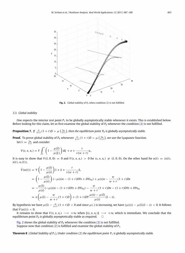
Fig. 2. Global stability of P0 when condition (2) is not fulfilled.
3.3. Global stability
One expects the interior rest point P1 to be globally asymptotically stable whenever it exists. This is established below.Before looking for this claim, let us first examine the global stability of P0 whenever the condition (2) is not fulfilled.
Proposition 7. If ww+r (1 + r)D > µ
sin1+r
, then the equilibrium point P0 is globally asymptotically stable.
Proof. To prove global stability of P0 whenever ww+r (1 + r)D > µ
sin1+r
, we use the Lyapunov function.
Set s :=sin1+r and consider
V (s, x, xr) = Y∫ s
s
1 −
µ(s)µ(ξ)
dξ + x +
rν(w + r)
xr .
It is easy to show that V (s, 0, 0) = 0 and V (s, x, xr) > 0 for (s, x, xr) = (s, 0, 0). On the other hand for u(t) = (s(t),x(t), xr(t)),
V (u(t)) = Y1 −
µ(s)µ(s)
s + x +
rν(w + r)
xr
=
1 −
µ(s)µ(s)
(−µ(s)x − (1 + r)DYs + DYsin) + µ(s)x −
w
w + r(1 + r)Dx
= −µ(s)µ(s)
(−µ(s)x − (1 + r)DYs + DYsin) −w
w + r(1 + r)Dx − (1 + r)DYs + DYsin
= x
µ(s) −w
w + r(1 + r)D
+ (1 + r)DY
µ(s) − µ(s)µ(s)
(s − s).
By hypothesis we have µ(s) −w
w+r (1 + r)D < 0 and since µ(.) is increasing, we have (µ(s)) − µ(s)(s − s) < 0. It followsthat V (u(t)) < 0.
It remains to show that V (s, x, xr) −→ +∞ when ||(s, x, xr)|| −→ +∞ which is immediate. We conclude that theequilibrium point P0 is globally asymptotically stable as required.
Fig. 2 shows the global stability of P0 whenever the condition (2) is not fulfilled.Suppose now that condition (2) is fulfilled and examine the global stability of P1.
Theorem 8 (Global Stability of P1). Under condition (2) the equilibrium point P1 is globally asymptotically stable.
494 M. Serhani et al. / Nonlinear Analysis: Real World Applications 12 (2011) 487–500
Proof. We prove the global stability of P1 by using the following Lyapunov function:
V (s, x, xr) := Yw + r
r
∫ s
s∗
1 −
µ(s∗)µ(ξ)
dξ +
w + rr
∫ x
x∗
1 −
x∗
ξ
dξ +
1v
∫ xr
xr∗
1 −
xr∗ξ
dξ .
It is easy to show that V (s∗, x∗, x∗r ) = 0, V (s, x, xr) > 0 for all (s, x, xr) = (s∗, x∗, x∗
r ), and that V (s, x, xr) −→ +∞ as(s, x, xr) −→ +∞.
It remains to show thatdVdt
(s(t), x(t), xr(t)) < 0 for all (s(t), x(t), xr(t)) = (s∗, x∗, x∗
r ),
dVdt
(s(t), x(t), xr(t)) = Yw + r
r
1 −
µ(s∗)µ(s)
s +
w + rr
1 −
x∗
x
x +
1v
1 −
xr∗xr
xr
=w + r
r
1 −
µ(s∗)µ(s)
[−µ(s)x − (1 + r)DYs + DYsin]
+
1 −
x∗
x
[w + r
rµ(s)x −
w + rr
(1 + r)Dx + (w + r)Dxr
]+
1 −
xr∗xr
[(1 + r)Dx − (w + r)Dxr ]
=w + r
r
1 −
µ(s∗)µ(s)
[−µ(s)x − (1 + r)DYs + DYsin]
+
1 −
x∗
x
[w + r
rµ(s)x −
w
r(1 + r)Dx
]+
1 −
x∗
x
[−(1 + r)Dx + (w + r)Dxr ] +
1 −
xr∗xr
[(1 + r)Dx − (w + r)Dxr ].
Set
A :=w + r
r
1 −
µ(s∗)µ(s)
[−µ(s)x − (1 + r)DYs + DYsin] +
1 −
x∗
x
[w + r
rµ(s)x −
w
r(1 + r)Dx
]and
B :=
1 −
x∗
x
[−(1 + r)Dx + (w + r)Dxr ] +
1 −
xr∗xr
[(1 + r)Dx − (w + r)Dxr ].
Then,dVdt
(s(t), x(t), xr(t)) = A + B.
Let us examine separately B and A. For B, set Q := (1 + r)x − (w + r)xr ; then we have
B =
1 −
xr∗xr
QD −
1 −
x∗
x
QD
= QD1xrx
(xrx∗− xx∗
r ).
But, since x∗r =
1+rw+r x
∗, we have
xrx∗− xx∗
r = xrx∗− x
1 + rw + r
x∗
= −Qx∗
w + r.
It follows, according to this fact, that
B = −Q 2Dx∗
xrxx∗
w + r< 0.
Return now to A:
A =w + r
r
1 −
µ(s∗)µ(s)
[−µ(s)x − (1 + r)DYs + DYsin] +
1 −
x∗
x
[w + r
rµ(s)x −
w
r(1 + r)Dx
]=
w + rr
µ(s) − µ(s∗)µ(s)
[DYsin − (1 + r)DYs − µ(s)x∗].
M. Serhani et al. / Nonlinear Analysis: Real World Applications 12 (2011) 487–500 495
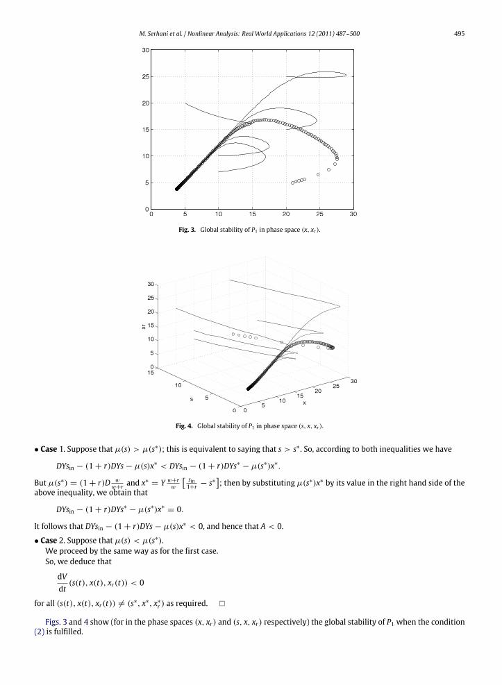
Fig. 3. Global stability of P1 in phase space (x, xr ).
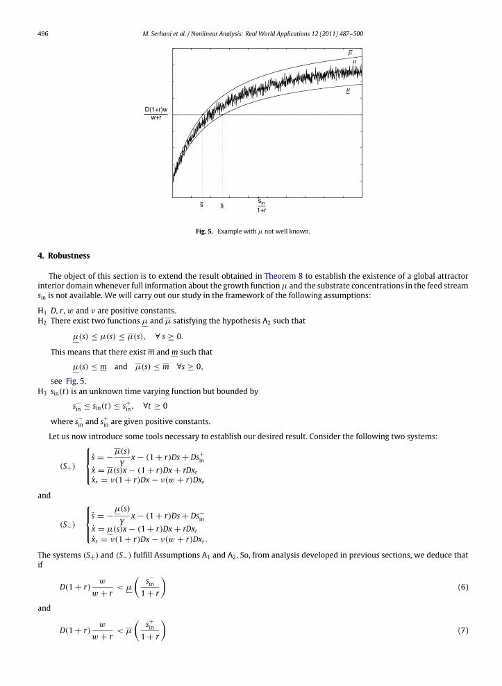
Fig. 4. Global stability of P1 in phase space (s, x, xr ).
• Case 1. Suppose that µ(s) > µ(s∗); this is equivalent to saying that s > s∗. So, according to both inequalities we have
DYsin − (1 + r)DYs − µ(s)x∗ < DYsin − (1 + r)DYs∗ − µ(s∗)x∗.
But µ(s∗) = (1 + r)D ww+r and x∗
= Y w+rw
sin1+r − s∗
; then by substituting µ(s∗)x∗ by its value in the right hand side of the
above inequality, we obtain that
DYsin − (1 + r)DYs∗ − µ(s∗)x∗= 0.
It follows that DYsin − (1 + r)DYs − µ(s)x∗ < 0, and hence that A < 0.
• Case 2. Suppose that µ(s) < µ(s∗).We proceed by the same way as for the first case.So, we deduce that
dVdt
(s(t), x(t), xr(t)) < 0
for all (s(t), x(t), xr(t)) = (s∗, x∗, x∗r ) as required.
Figs. 3 and 4 show (for in the phase spaces (x, xr) and (s, x, xr) respectively) the global stability of P1 when the condition(2) is fulfilled.
496 M. Serhani et al. / Nonlinear Analysis: Real World Applications 12 (2011) 487–500
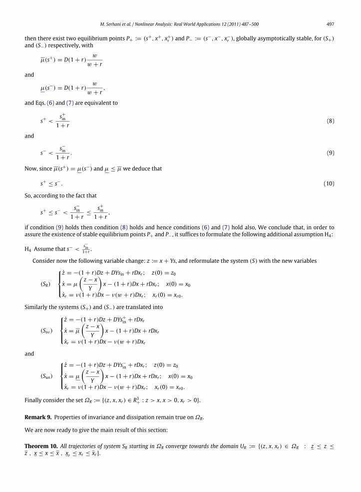
Fig. 5. Example with µ not well known.
4. Robustness
The object of this section is to extend the result obtained in Theorem 8 to establish the existence of a global attractorinterior domainwhenever full information about the growth functionµ and the substrate concentrations in the feed streamsin is not available. We will carry out our study in the framework of the following assumptions:
H1 D, r , w and ν are positive constants.H2 There exist two functions µ and µ satisfying the hypothesis A2 such that
µ(s) ≤ µ(s) ≤ µ(s), ∀ s ≥ 0.
This means that there existm and m such that
µ(s) ≤ m and µ(s) ≤ m ∀s ≥ 0,
see Fig. 5.H3 sin(t) is an unknown time varying function but bounded by
s−in ≤ sin(t) ≤ s+in, ∀t ≥ 0
where s−in and s+in are given positive constants.
Let us now introduce some tools necessary to establish our desired result. Consider the following two systems:
(S+)
s = −
µ(s)Y
x − (1 + r)Ds + Ds+inx = µ(s)x − (1 + r)Dx + rDxrxr = ν(1 + r)Dx − ν(w + r)Dxr
and
(S−)
s = −
µ(s)
Yx − (1 + r)Ds + Ds−in
x = µ(s)x − (1 + r)Dx + rDxrxr = ν(1 + r)Dx − ν(w + r)Dxr .
The systems (S+) and (S−) fulfill Assumptions A1 and A2. So, from analysis developed in previous sections, we deduce thatif
D(1 + r)w
w + r< µ
s−in
1 + r
(6)
and
D(1 + r)w
w + r< µ
s+in
1 + r
(7)
M. Serhani et al. / Nonlinear Analysis: Real World Applications 12 (2011) 487–500 497
then there exist two equilibrium points P+ := (s+, x+, x+r ) and P− := (s−, x−, x−
r ), globally asymptotically stable, for (S+)and (S−) respectively, with
µ(s+) = D(1 + r)w
w + r
and
µ(s−) = D(1 + r)w
w + r,
and Eqs. (6) and (7) are equivalent to
s+ <s+in
1 + r(8)
and
s− <s−in
1 + r. (9)
Now, since µ(s+) = µ(s−) and µ ≤ µ we deduce that
s+ ≤ s−. (10)
So, according to the fact that
s+ ≤ s− <s−in
1 + r≤
s+in1 + r
,
if condition (9) holds then condition (8) holds and hence conditions (6) and (7) hold also, We conclude that, in order toassure the existence of stable equilibrium points P+ and P−, it suffices to formulate the following additional assumption H4:
H4 Assume that s− <s−in1+r .
Consider now the following variable change: z := x + Ys, and reformulate the system (S) with the new variables
(SR)
z = −(1 + r)Dz + DYsin + rDxr; z(0) = z0
x = µ
z − xY
x − (1 + r)Dx + rDxr; x(0) = x0
xr = ν(1 + r)Dx − ν(w + r)Dxr; xr(0) = xr0.
Similarly the systems (S+) and (S−) are translated into
(Sov)
z = −(1 + r)Dz + DYs+in + rDxr
x = µ
z − xY
x − (1 + r)Dx + rDxr
xr = ν(1 + r)Dx − ν(w + r)Dxr
and
(Sun)
z = −(1 + r)Dz + DYs−in + rDxr; z(0) = z0
x = µ
z − xY
x − (1 + r)Dx + rDxr; x(0) = x0
xr = ν(1 + r)Dx − ν(w + r)Dxr; xr(0) = xr0.
Finally consider the set ΩR := (z, x, xr) ∈ R3+
: z > x, x > 0, xr > 0.
Remark 9. Properties of invariance and dissipation remain true on ΩR.
We are now ready to give the main result of this section:
Theorem 10. All trajectories of system SR starting in ΩR converge towards the domain UR := (z, x, xr) ∈ ΩR : z ≤ z ≤
z , x ≤ x ≤ x , xr ≤ xr ≤ xr.
498 M. Serhani et al. / Nonlinear Analysis: Real World Applications 12 (2011) 487–500
Proof. It is clear that Sun ≤ SR ≤ Sov in the sense that the vector field of SR is bounded below by the vector field of Sun andbounded above by one of the systems Sov . Furthermore, since the Jacobian matrix of the systems (Sov) given by
J(Sov) =
−(1 + r)D 0 rDµ′
z−xY
x
Yµ
z − xY
− (1 + r)D −
µ′ z−x
Y
x
YrD
0 ν(1 + r)D −ν(w + r)D
and the Jacobian matrix of the systems (Sun) given by
J(Sun) =
−(1 + r)D 0 rDµ′
z−xY
x
Yµ
z − xY
− (1 + r)D −
µ′ z−x
Y
x
YrD
0 ν(1 + r)D −ν(w + r)D
are nonnegative outside the diagonal elements (µ′ andµ′ are nonnegative according to assumption A2), then these systemsare cooperative (see for e.g. [16] and [17]). Therefore, by using arguments of cooperative inequalities (see Appendix B of [17]),we obtain that if
u(t, u0) := (z(t), x(t), xr(t)) ∈ R+3 / (z(0), x(0), xr(0)) = u0 := (z0, x0, xr0),
is the flow of (SR) and similarly u(t, u0) and u(t, u0) are respectively the flows of (Sov) and (Sun) starting at the same pointu0, then
u(t, u0) ≤ u(t, u0) ≤ u(t, u0) ∀t ≥ 0. (11)
On the other hand, with the change of variable z, the asymptotical global stable equilibrium points P− = (s−, x−, x−r )
and P+ = (s+, x+, x+r ) for the systems (S−) and (S+), respectively, are translated into asymptotical global stable equilibrium
points P := (z, x, xr) and P := (z, x, xr) in the new systems (Sov) and (Sun) respectively. In other words, all trajectories ofsystem Sun (respectively Sov) starting in ΩR, converge towards P (respectively P). Hence, according to (11) we conclude thatall trajectories of system (SR) starting in ΩR converge towards a domain UR bounded above by P and below by P:
UR := (z, x, xr) ∈ ΩR : z ≤ z ≤ z, x ≤ x ≤ x, xr ≤ xr ≤ xr
as required.
It remains now to deduce the domain U towards which all trajectories of system (S) converge. To do this, wemust definethe variables of system (S) from those of (SR). Let
s− :=z − xY
; s :=z − xY
; s+ :=z − xY
(12)
and
x−:= x; x+
:= x; x−
r := xr; x+
r := xr (13)
where P = (z, x, xr), (z, x, xr) and P = (z, x, xr) are respectively the equilibriumpoint of system (Sun), a trajectory of system(SR) and the equilibrium point of system (Sov). Hence, P corresponds to the equilibrium point of (S−), P− = (s−, x−, x−
r ),and P corresponds to the equilibrium point of (S+), P+ = (s+, x+, x+
r ).We are now ready to establish the following result for a trajectory (s, x, xr) of system (S).
Corollary 11. Each trajectory (s, x, xr) of system (S) starting in Ω converges towards the domain U := (s, x, xr) ∈ Ω :
s− − ∆ ≤ s ≤ s+ + ∆ , x−≤ x ≤ x+ , x−
r ≤ xr ≤ x+r , where ∆ :=
x+−x−Y .
Proof. From the robustness Theorem 10, we know that there exists T > 0 such that
z ≤ z(t) ≤ z; x ≤ x(t) ≤ x; xr ≤ xr(t) ≤ xr ∀t ≥ T
for each trajectory (z, x, xr) of system (SR). According to those inequalities, if (s, x, xr) is a trajectory of system (S) obtainedfrom (z, x, xr) by the transformations (12) and (13), then
Ys + x ≤ Ys+ + x+
which implies that
s ≤x+
− xY
+ s+
M. Serhani et al. / Nonlinear Analysis: Real World Applications 12 (2011) 487–500 499
and hence
s ≤x+
− x−
Y+ s+.
Conversely, following the same route, we obtain that
s ≥x−
− x+
Y+ s−.
We conclude that
s− − ∆ ≤ s ≤ s+ + ∆, (14)
where ∆ :=x+−x−
Y . As required.
5. Reduction of the stability region U
The purpose of this section is to give a practical tool for reducing the size of stability domain U . The idea is to find anadequate value of the recycle rate r for which U reaches its minimal size (volume) value. Assume that:
H5 0 ≤ r ≤ R, where R is the maximum level where r can be reached.
Theorem 12. We can reduce the size of stability domain U by increasing the recycle rate r. Furthermore, under additionalassumption H5, the minimal size of U is achieved when r = R and is given by
LR =w + R
Y 2R2(1 + R)(s+in − s−in)
2(s− − s+) + 2w + RY 2R2
(s+in − s−in)(s−
− s+)2 +(1 + R)(w + R)
Y 2R2(s− − s+)3.
Proof. First, let us calculate the size L of stability domain U . We have that
L := (s− − s+)(x+− x−)(x+
r − x−
r )
and remark that, according to (10), (s− − s+) ≥ 0. On the other hand, taking account of equilibrium equation (5), we cancalculate (x+
− x−) by using (s− − s+). Indeed,
(x+− x−) =
w + rYr
[s+in − s−in1 + r
+ s− − s+]
and according to equilibrium equation (3), we can calculate (x+r − x−
r ) by using (s− − s+). Indeed,
(x+
r − x−
r ) =1 + rw + r
(x+− x−)
=1 + rYr
[s+in − s−in1 + r
+ s− − s+]
.
Hence,
L =w + r
Y 2r2(1 + r)(s+in − s−in)
2(s− − s+) + 2w + rY 2r2
(s+in − s−in)(s−
− s+)2 +(1 + r)(w + r)
Y 2r2(s− − s+)3.
It is easy to prove, by studying variations of w+rY2r2(1+r)
, 2w+rY2r2
and (1+r)(w+r)Y2r2
with respect to r , that those functions aredecreasing. Now, it remains to show that if r increases then (s− − s+) decreases. Indeed,
(s− − s+) = µ−1Dw
1 + rw + r
− µ−1
Dw
1 + rw + r
= µ−1
Dw
1 + rw + r
− µ−1(0) + µ−1(0) − µ−1(0) + µ−1(0) − µ−1
Dw
1 + rw + r
.
Using Lipshitz properties of µ−1 and µ−1 and the fact that µ−1(0) = µ−1(0) = 0, we obtain
(s− − s+) ≤ (k1 + k2)Dw1 + rw + r
where k1 and k2 are, respectively, the Lipshitz constant of µ−1 and µ−1. So, since Dw 1+rw+r is also decreasing with respect to
r then (s− − s+) is decreasing with respect to r and hence L is decreasing with respect to r . We conclude that we can reduce
500 M. Serhani et al. / Nonlinear Analysis: Real World Applications 12 (2011) 487–500
the size of stability domain U by increasing the recycle rate r . Furthermore, since 0 ≤ r ≤ R, then the minimal size of U isobtained when r = R and is given by
LR =w + R
Y 2R2(1 + R)(s+in − s−in)
2(s− − s+) + 2w + RY 2R2
(s+in − s−in)(s−
− s+)2 +(1 + R)(w + R)
Y 2R2(s− − s+)3.
Corollary 13. Using Lipshitz properties of µ−1 and µ−1, we can give an estimation of LR as
L ≤ (k1 + k2)Dw
Y 2R2
[(s+in − s−in)
2+ 2
Dw(1 + R)2
w + R(s+in − s−in)(k1 + k2) +
(1 + R)4D2w2
(w + R)2(k1 + k2)2
].
Proof. It suffices to substitute, in the expression for LR, (s− − s+) by the Lipshitz inequality
(s− − s+) ≤ (k1 + k2)Dw1 + rw + r
,
proved in the proof of the previous theorem.
6. Conclusion
This work is concerned with an activated sludge problem.We have proved that in the case where all parameters are wellknown, the model admits a unique global stable equilibrium point. Otherwise, if information about the bacterium specificgrowth functionµ and the concentration in the feed stream sin is not available, the robustness analysis leads to the existenceof a stability domain U . Finally, we propose a simple way to reduce the size (volume) of the stability domain by increasingthe recycle rate r , and hence the stability domain reaches its minimal size when r achieves its maximum level. This workmay be extended to take account of the cost of the recycle operation. This will be our next area of interest, using optimalcontrol theory.
Acknowledgements
The first author was supported by the University Agency of Francophony (AUF).
References
[1] J.F. Andrews, Kinetic models of biological waste treatment process, Biotech. Bioeng. Symp. 2 (1971) 5–34.[2] J.F. Busby, J.F. Andrews, Dynamicmodelling and control strategies for the activated sludge process, J. Water. Pollut. Control Fed. 47 (1975) 1055–1080.[3] M.Z. Hadj-Sadok, J.L. Gouzé, Estimation of uncertainmodels of activated sludge processeswith interval observers, J. Process Control 11 (2001) 299–310.[4] M.Z. Hadj-Sadok, J.L. Gouzé, Estimation of uncertain models of activated sludge processes with interval observers, Doctorat Thesis, 2001.[5] S. Marsili-Libelli, Optimal control of the activated sludge process, Trans. Inst. Meas. Control 6 (1984) 146–152.[6] M. Serhani, N. Raissi, P. Cartigny, Robust feedback control design for a nonlinear wastewater treatment model, J. Math. Model. Nat. Phenom. 4 (5)
(2009) 128–143.[7] C. Gómez-Quintero, I. Queinnec, Robust estimation for an uncertain linear model of an activated sludge process, in: Proc. of the IEEE Conference on
Control Applications, CCA, 18–20 December, Glasgow, UK, 2002.[8] A. Rapaport, J. Harmand, Robust regulation of a class of partially observed nonlinear continuous bioreactors, J. Process Control 12 (2) (2002) 291–302.[9] J.F. Andrews, Dynamics and control of wastewater systems, Water Quality Management Library 6 (1998).
[10] C.R. Curds, Computer simulation of microbial population dynamics in the activated sludge process, Water Res. 5 (1971) 1049–1066.[11] M.K. Rangla, K.J. Burnham, L. Coyle, R.I. Stephens, Simulation of activated sludge process control strategies, Simulation ’98. International Conference
on (Conf. Publ. No. 457), 30 Sept.–2 Oct, 1998, pp. 152–157.[12] D. Dochain, M. Perrier, Control design for nonlinear wastewater treatment processes, Water. Sci. Technol. 11–12 (1993) 283–293.[13] D. Dochain, M. Perrier, Dynamical modelling, analysis, monitoring and control design for nonlinear bioprocess, in: T. Scheper (Ed.), in: Advances in
Biochemical and Biotechnology, vol. 56, Springer-Verlag, 1997, pp. 147–197.[14] A. Martínez, C. Rodríguez, M.E. Vázquez-Méndez, Theoretical and numerical analysis of an optimal control problem related to wastewater treatment,
SIAM J. Control Optim. 38 (5) (2000) 1534–1553.[15] B. Haegeman, C. Lobry, J. Harmand, Modeling bacteria flocculation as density-dependent growth, AIChE J. 53 (2) (2007) 535–539.[16] H.L. Smith, Monotone Dynamical Systems: An Introduction to the Theory of Competitive and Cooperative Systems, American Mathematical Society,
1995.[17] H.L. Smith, P. Waltman, The Theory of the Chemostat, Cambridge University Press, Cambridge, 1995.