Dynamic Voltage/Frequency Scaling and Power-Gating of Network-on-Chip with

Machine Learning

A thesis presented to

the faculty of

the Russ College of Engineering and Technology of Ohio University

In partial fulfillment

of the requirements for the degree

Master of Science

Mark A. Clark

May 2019

© 2019 Mark A. Clark. All Rights Reserved.

2

This thesis titled

Dynamic Voltage/Frequency Scaling and Power-Gating of Network-on-Chip with

Machine Learning

by

MARK A. CLARK

has been approved for

the School of Electrical Engineering and Computer Science

and the Russ College of Engineering and Technology by

Avinash Karanth

Professor of Electrical Engineering and Computer Science

Dennis Irwin

Dean, Russ College of Engineering and Technology

3

Abstract

CLARK, MARK A., M.S., May 2019, Electrical Engineering

Dynamic Voltage/Frequency Scaling and Power-Gating of Network-on-Chip with

Machine Learning (89 pp.)

Director of Thesis: Avinash Karanth

Network-on-chip (NoC) continues to be the preferred communication fabric in

multicore and manycore architectures as the NoC seamlessly blends the resource efficiency

of the bus with the parallelization of the crossbar. However, without adaptable power

management the NoC suffers from excessive static power consumption at higher core

counts. Static power consumption will increase proportionally as the size of the NoC

increases to accommodate higher core counts in the future. NoC also suffers from excessive

dynamic energy as traffic loads fluctuate throughout the execution of an application. Power-

gating (PG) and Dynamic Voltage and Frequency Scaling (DVFS) are two highly effective

techniques proposed in literature to reduce static power and dynamic energy in the NoC

respectively. DVFS is a popular technique that allows dynamic energy to be saved but may

potentially lead to a loss in throughput. Power-gating allows static power to be saved but

can introduce new problems incurred by isolating network routers. Further complications

include the introduction of long wake-up delays and break-even times. However, both

DVFS and power-gating are critical for realizing energy proportional computing as core

counts race into the hundreds for multi-cores.

In this thesis, we propose two distinct but related techniques that enable energy-

proportional computing for NoC. We first propose LEAD - Learning-enabled Energy-

Aware Dynamic voltage/frequency scaling for NoC architectures. LEAD applies machine

learning (ML) techniques to enable improvements in both energy and performance with

reduced overhead cost. This allows LEAD to enact a proactive energy management

strategy that relies on an offline trained regression model while also providing a wide

4

variety of voltage/frequency (VF) pairs. In this work, we will refer to various VF pairs

as modes. LEAD groups each router and the router’s outgoing links locally into the

same V/F domain allowing energy management at a finer granularity without additional

timing complications and overhead. We then build on LEAD and propose DozzNoC, an

adaptable power management technique that effectively combines LEAD with a partially

non-blocking power-gating technique. This allows DozzNoC to target both static power

and dynamic energy simultaneously, thereby enabling energy proportional computing. Our

ML DVFS techniques from LEAD are applied on top of a partially non-blocking power-

gated scheme that uses real valued wake-up/switching delays. DozzNoC also allows

independently power-gated or voltage scaled routers such that each router and its outgoing

links share the same voltage/frequency domain.

We evaluate both LEAD and DozzNoC using trace files generated from PARSEC 2.1

and Splash-2 benchmark suits. Trace files are gathered at various network sizes and across

two different network topologies. For a 64 core 4 × 4 concentrated mesh (CMesh) network,

simulation results show that LEAD can achieve an average of 17% dynamic energy savings

for an average loss of only 4% throughput. Our simulation results for DozzNoC on an 8 ×

8 mesh network show that for an average decrease of 7% in throughput, we can achieve an

average dynamic energy savings of 25% and an average static power reduction of 53%.

5

Acknowledgments

I thank my advisor, Dr. Avinash Karanth for the support, guidance, and motivation he

provided. I also want to thank the many wonderful friends I made throughout my time at

Ohio University, even if we have since gone our own ways in life.

6

Table of Contents

Page

Abstract . . . . . . . . . . . . . . . . . . . . . . . . . . . . . . . . . . . . . . . . . 3

Acknowledgments . . . . . . . . . . . . . . . . . . . . . . . . . . . . . . . . . . . . 5

List of Tables . . . . . . . . . . . . . . . . . . . . . . . . . . . . . . . . . . . . . . 8

List of Figures . . . . . . . . . . . . . . . . . . . . . . . . . . . . . . . . . . . . . . 9

List of Acronyms . . . . . . . . . . . . . . . . . . . . . . . . . . . . . . . . . . . . 11

1 Introduction . . . . . . . . . . . . . . . . . . . . . . . . . . . . . . . . . . . . . 131.1 Integrated Circuits to Multicores . . . . . . . . . . . . . . . . . . . . . . . 131.2 Energy Proportional Computing and NoC . . . . . . . . . . . . . . . . . . 161.3 Dynamic Voltage and Frequency Scaling for Multicores . . . . . . . . . . . 191.4 Power-gating for Multicores . . . . . . . . . . . . . . . . . . . . . . . . . 211.5 Benefits of Machine Learning . . . . . . . . . . . . . . . . . . . . . . . . 231.6 Major Contributions . . . . . . . . . . . . . . . . . . . . . . . . . . . . . . 241.7 Thesis Organization . . . . . . . . . . . . . . . . . . . . . . . . . . . . . . 25

2 LEAD: Offline Trained Proactive DVFS for NoC . . . . . . . . . . . . . . . . . 272.1 Related Works . . . . . . . . . . . . . . . . . . . . . . . . . . . . . . . . . 272.2 LEAD Architecture . . . . . . . . . . . . . . . . . . . . . . . . . . . . . . 33

2.2.1 Operating V/F Modes . . . . . . . . . . . . . . . . . . . . . . . . 332.3 DVFS Models and Implementation . . . . . . . . . . . . . . . . . . . . . . 34

2.3.1 DVFS Implementation . . . . . . . . . . . . . . . . . . . . . . . . 372.4 Machine Learning for DVFS . . . . . . . . . . . . . . . . . . . . . . . . . 39

3 DozzNoC: Combination of ML based DVFS and Power-Gating for NoC . . . . . 413.1 Related Works . . . . . . . . . . . . . . . . . . . . . . . . . . . . . . . . . 413.2 DozzNoC Architecture . . . . . . . . . . . . . . . . . . . . . . . . . . . . 46

3.2.1 Operational States . . . . . . . . . . . . . . . . . . . . . . . . . . 483.3 Power-Gated DVFS Models . . . . . . . . . . . . . . . . . . . . . . . . . 503.4 Machine Learning for PG-DVFS . . . . . . . . . . . . . . . . . . . . . . . 55

4 Performance Evaluation . . . . . . . . . . . . . . . . . . . . . . . . . . . . . . . 584.1 LEAD Simulation Methodology . . . . . . . . . . . . . . . . . . . . . . . 58

4.1.1 LEAD Model Variants . . . . . . . . . . . . . . . . . . . . . . . . 604.1.2 LEAD Mode Breakdown . . . . . . . . . . . . . . . . . . . . . . . 61

4.2 LEAD ML Simulation Methodology . . . . . . . . . . . . . . . . . . . . . 62

7

4.2.1 LEAD Feature Engineering . . . . . . . . . . . . . . . . . . . . . 634.2.2 LEAD ML Accuracy . . . . . . . . . . . . . . . . . . . . . . . . . 66

4.3 DozzNoC Simulation Methodology . . . . . . . . . . . . . . . . . . . . . 674.3.1 DozzNoC Model Variants . . . . . . . . . . . . . . . . . . . . . . 694.3.2 DozzNoC Mode Breakdown . . . . . . . . . . . . . . . . . . . . . 71

4.4 DozzNoC ML Simulation Methodology . . . . . . . . . . . . . . . . . . . 724.4.1 DozzNoC Feature Engineering . . . . . . . . . . . . . . . . . . . . 73

4.5 LEAD Results . . . . . . . . . . . . . . . . . . . . . . . . . . . . . . . . . 754.5.1 LEAD Energy and Throughput . . . . . . . . . . . . . . . . . . . . 75

4.6 DozzNoC Results . . . . . . . . . . . . . . . . . . . . . . . . . . . . . . . 764.6.1 DozzNoC Throughput, Static Power, and Dynamic Energy . . . . . 77

5 Conclusions and Future Work . . . . . . . . . . . . . . . . . . . . . . . . . . . . 81

References . . . . . . . . . . . . . . . . . . . . . . . . . . . . . . . . . . . . . . . . 83

8

List of Tables

Table Page

3.1 DozzNoC’s Reduced Feature Set [16] . . . . . . . . . . . . . . . . . . . . . . 564.1 LEAD Benchmarks . . . . . . . . . . . . . . . . . . . . . . . . . . . . . . . . 584.2 Multi2sim Parameters . . . . . . . . . . . . . . . . . . . . . . . . . . . . . . . 594.3 Dynamic Energy Per Hop (Modes 1-5) [17]©2018 ACM . . . . . . . . . . . . 604.4 Full LEAD Feature Set . . . . . . . . . . . . . . . . . . . . . . . . . . . . . . 654.5 Full LEAD Feature Set (Cont.) . . . . . . . . . . . . . . . . . . . . . . . . . . 664.6 LEAD-τ Mode Selection Accuracy [17]©2018 ACM . . . . . . . . . . . . . . 674.7 DozzNoC Benchmarks . . . . . . . . . . . . . . . . . . . . . . . . . . . . . . 684.8 Static Power and Dynamic Energy Per Hop for Active State Operational Modes

[16] . . . . . . . . . . . . . . . . . . . . . . . . . . . . . . . . . . . . . . . . 70

9

List of Figures

Figure Page

1.1 Rapid growth of processor performance from increased clock speed to multi-core processors [46]. . . . . . . . . . . . . . . . . . . . . . . . . . . . . . . . 15

1.2 Various network topologies ranging from the bus to a hypercube. . . . . . . . . 171.3 Depiction of static power becoming the majority of power consumption in the

NoC as technology size decreases. [9]. . . . . . . . . . . . . . . . . . . . . . . 181.4 Depiction of DVFS being applied at various granularities ranging from per

network to per element. . . . . . . . . . . . . . . . . . . . . . . . . . . . . . . 201.5 An example of power-gating applied to the NoC where the router modification,

handshaking, and router pipeline are shown from Power-Punch [13]. . . . . . . 222.1 An example DVS link is shown in part (a), while a history-based DVS

algorithm is shown in part (b) [51]. . . . . . . . . . . . . . . . . . . . . . . . . 302.2 A Threshold and PI controller Finite State Machine (FSM) are shown in (a),

while a Greedy controller FSM is shown in (b) [30]. . . . . . . . . . . . . . . . 312.3 An example of simultaneous power, temperature, and performance manage-

ment using Q-learning [52]. . . . . . . . . . . . . . . . . . . . . . . . . . . . . 322.4 We apply LEAD to a CMesh with 16 routers and 64 cores. We use on chip

voltage regulators that can adjust the supply voltage between 0.8V and 1.2V,allowing us to apply DVFS to individual routers and their corresponding links[17]©2018 ACM. . . . . . . . . . . . . . . . . . . . . . . . . . . . . . . . . . 34

2.5 The architecture as well as all additional units required for reactive or proactivemode selection are shown in (a). A simple voltage regulator setup that allowsthe selection of voltage levels in the range of 0.8V to 1.2V for every router andits’ associated outgoing links is shown in (b) [17]©2018 ACM. . . . . . . . . . 35

2.6 LEAD-τ uses a predicted input buffer utilization to select the optimal modeper epoch. LEAD-∆ uses a predicted change in input buffer utilization tomove in the direction of the optimal mode per epoch. LEAD-G incorporatesboth energy and throughput into the label and moves up/down adjacent modes(based on exploration direction) such that energy divided by throughput isminimized [17]©2018 ACM. . . . . . . . . . . . . . . . . . . . . . . . . . . . 38

3.1 The difference in network component sizes between a Single-NoC and a Multi-NoC [19]. . . . . . . . . . . . . . . . . . . . . . . . . . . . . . . . . . . . . . 43

3.2 The NoRD network bypass ring is shown in (a), the router bypass datapath isshown in (b), and the network interface datapath is shown in (c) [11]. . . . . . . 44

3.3 Four seperate DarkNoC layers are shown in (a), a single DarkNoC layer isshown in (b), and DarkNoC routers are shown in (c) [8]. . . . . . . . . . . . . 46

3.4 We apply DozzNoC to both a CMesh in (a), as well as a mesh in (b). The routermicroarchitecture for a mesh topology is shown in (c) [16]. . . . . . . . . . . . 47

10

3.5 Our version of Power Punch acts as a baseline and is shown in (a). LEAD-τhas only one state, the active state; however active routers may operate at oneof five different voltage levels (b). DozzNoC has three states and when a routeris active it may operate at one of five different voltage levels as shown in (c) [16]. 49

3.6 DozzNoC mode selection is shown in (a), while LEAD-τ mode selection isshown in (b) [16]. . . . . . . . . . . . . . . . . . . . . . . . . . . . . . . . . . 50

3.7 A walkthrough example showing the difference in active state mode selectionacross two epochs for a dummy network [16]. . . . . . . . . . . . . . . . . . . 53

4.1 The throughput loss and dynamic energy savings across multiple LEAD-τvariants with an epoch size of 500 cycles [17]©2018 ACM. . . . . . . . . . . . 61

4.2 The time routers and links spent in each mode for all LEAD models across alltest traces [17]©2018 ACM. . . . . . . . . . . . . . . . . . . . . . . . . . . . 62

4.3 The change in throughput, dynamic energy, and latency of DozzNoC at variousepoch sizes compared to a baseline DozzNoC model with an epoch size of 100cycles [16]. . . . . . . . . . . . . . . . . . . . . . . . . . . . . . . . . . . . . 71

4.4 A breakdown of predicted operational modes while in an active state for an 8× 8 mesh network for DozzNoC (a), LEAD-τ (b), and ML+TURBO (c) [16]. . 72

4.5 The results of DozzNoC single feature mode selection accuracy testing [16]. . . 734.6 The throughput, latency, dynamic energy savings, static power savings and

EDP of DozzNoC-5 versus DozzNoC-41 [16]. . . . . . . . . . . . . . . . . . . 744.7 The throughput (a) and Normalized Dynamic Energy (b) for all LEAD models

compared against baseline and greedy [17]©2018 ACM. . . . . . . . . . . . . 764.8 DozzNoC throughput for CMesh architecture at epoch size of 500 cycles (a).

DozzNoC normalized static and dynamic energy for CMesh at epoch size of500 cycles at high load (b). DozzNoC normalized static and dynamic energyfor CMesh at epoch size of 500 cycles at low load (c) [16]. . . . . . . . . . . . 78

4.9 DozzNoC throughput for mesh architecture at epoch size of 500 cycles (a).DozzNoC normalized static and dynamic energy for mesh at epoch size of 500cycles at high load (b). DozzNoC normalized static and dynamic energy formesh at epoch size of 500 cycles at low load (c) [16]. . . . . . . . . . . . . . . 79

11

List of Acronyms

BW - Buffer Write

CMesh - Concentrated Mesh

DOR - Dimension Order Routing

DozzNoC - Partially non-blocking Power-Gating with ML based DVFS

DVS - Dynamic Voltage Scaling

DVFS - Dynamic Voltage and Frequency Scaling

HPC - High-Performance Computing

HVt - High Threshold Voltage

IC - Integrated Circuit

LEAD - Learning-enabled Energy-Aware Dynamic voltage/frequency scaling

LVt - Low Threshold Voltage

ML - Machine Learning

MOSFET - Metal-Oxide-Semiconductor Field-Effect Transistor

NoC - Network-on-Chip

NVt - Normal Threshold Voltage

PG - Power-Gating

RC - Router Computation

RL - Reinforcement Learning

SA - Switch Allocation

SCC - Single-chip Cloud Computer

SSI - Small-Scale Integration

ST - Switch Traversal

T-Breakeven - Breakeven Time

T-Wakeup - Wake-up Delay

ULSI - Ultra-Large-Scale Integration

12

VA - Virtual Channel Allocation

VC - Virtual Channel

VFI - Voltage Frequency Island

13

1 Introduction

1.1 Integrated Circuits to Multicores

1The modern multi-core processor is a result of several technological advancements

that began with the development of the integrated circuit (IC). The IC, a collection of

microelectronic components or circuits fabricated onto the same microchip [36], were

enabled largely due to the discovery of the transistor. A transistor is a semiconductor

that acts like an electronic switch in most cases [23, 53, 60] but may also be used for

signal amplification. At the time of its discovery almost 70 years ago, the transistor

was large and made with vacuum tubes. The number of transistors contained within

an IC was negligible and in the small-scale integration (SSI) range. However, in the

next few decades, MOSFET (metal-oxide-semiconductor field-effect transistor) scaling

following Moore’s Law [42] had allowed the size of the transistor to be drastically

reduced. Moore’s Law [42, 50] is an observation from Gordon Moore which states that

the number of transistors per square inch on an IC will double every year, which eventually

changed into doubling every 18 months. This allowed the number of transistors packed

onto IC’s to grow into the ultra-large-scale integration (ULSI) range. In 1974, Robert

H. Dennard noted that as transistor size decreased, power density remained constant

[54]. Dennard Scaling meant that as technology size decreased there would be an ever-

increasing need for power management strategies. At larger technology sizes, dynamic

power constituted the majority of the power consumed by the chip. Therefore, early

power management strategies focused on the reduction of dynamic energy, the energy

that is expended due to transistor switching [7, 20, 41, 51]. However, power consumption

has not remained proportional to area as Dennard failed to consider leakage current. At

1 Some material including figures, sentences, and paragraphs are used verbatim from prior publications[17, 26] with permission©2018 ACM and©2018 IEEE as well as a submitted publication awaiting decision[16]

14

smaller technology sizes, leakage current has caused static power to become the dominant

source of power consumption in the IC [10, 25, 28, 43]. Modern integrated circuits known

as microprocessors contain several billions of transistors. Examples of microprocessors

include the many core TILE-Gx [47], the Kalray MPPA-256 [21], and the 336-core Ambric

Am2045 [33]. With these astronomical number of transistors, there is an urgent need for

power management strategies. Such strategies must enable energy proportional computing

through the reduction of both static power and dynamic energy.

The multi-core processor is an advanced microprocessor that contains multiple

independent processing units. Each individual processing unit can execute separate

instructions from multiple threads in parallel. Processing cores/threads can also work

together on the same application or task by dividing parallel instructions among the cores.

The popularity of multi-core processors is a direct result of the ever-increasing demand

for computational power to run high-performance computing (HPC) applications. Such

applications range from simulations in astrophysics or biology, to large artificial neural

networks in machine learning, to cloud computing [34, 38, 49].

There are essentially two different methods of increasing the computational power

of the processor, the first involves increasing clock speed. Instructions are executed on

the rising or falling edge of the clock, therefore if the clock frequency is increased the

throughput of the processor will rise. This can be accomplished by increasing the power

consumption of the processor as power and frequency are directly related. However, due

to Moore’s Law and Dennard Scaling, there is an upper limit to this growth. Eventually

the amount of power consumed to raise the clock frequency will outweigh any additional

performance benefits. Intel and other chip manufacturers saw this phenomenon around 3-4

GHz as processor designers ran into the power-wall [46]. As this upper limit was reached,

a new method emerged to increase computational throughput. Instead of increasing

the clock frequency, several lower frequency processing units were built onto the same

15

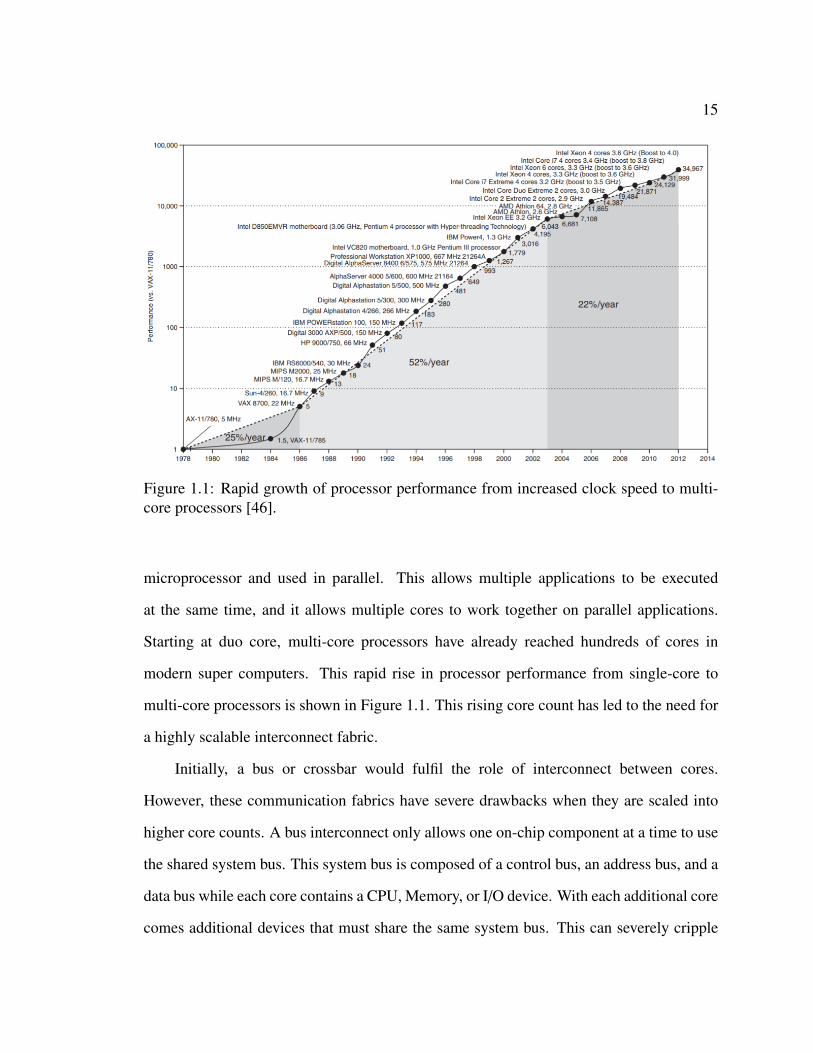
Figure 1.1: Rapid growth of processor performance from increased clock speed to multi-core processors [46].

microprocessor and used in parallel. This allows multiple applications to be executed

at the same time, and it allows multiple cores to work together on parallel applications.

Starting at duo core, multi-core processors have already reached hundreds of cores in

modern super computers. This rapid rise in processor performance from single-core to

multi-core processors is shown in Figure 1.1. This rising core count has led to the need for

a highly scalable interconnect fabric.

Initially, a bus or crossbar would fulfil the role of interconnect between cores.

However, these communication fabrics have severe drawbacks when they are scaled into

higher core counts. A bus interconnect only allows one on-chip component at a time to use

the shared system bus. This system bus is composed of a control bus, an address bus, and a

data bus while each core contains a CPU, Memory, or I/O device. With each additional core

comes additional devices that must share the same system bus. This can severely cripple

16

any potential performance gains. This means that while the bus is extremely resource

efficient, its performance is not scalable into higher core counts. The crossbar switch is

a non-blocking interconnect. A crossbar allows multiple components to use dedicated

channels without interrupting the connectivity of other components. However, this type

of interconnect uses vast amounts of wires and switch points at higher core counts. This

implies that the crossbar interconnect is not easily scalable in terms of on-chip area and

resource in-efficiency. Therefore, a newer communication fabric known as the Network-

on-Chip (NoC) has emerged that seeks to combine the resource efficiency of the bus with

the parallelizable nature of the crossbar.

1.2 Energy Proportional Computing and NoC

The NoC allows several cores to communicate and work in parallel through the usage

of multiple routers and links. These routers and links may be arranged in various physical

layouts or network topologies which belong to two types of networks. The first type of

network is called a direct network in which every node is both a terminal and a switch.

This differs from an indirect network in which nodes may be either switches or terminals

[1]. The simplest direct network is the mesh topology wherein routers and links form a

grid-like pattern. Each core is connected to a dedicated router which is used to send and

receive data among cores. A concentrated mesh (CMesh) topology is similar to a mesh in

that routers and links are arranged in a grid-like pattern. However, the CMesh differs from

a mesh because multiple cores share a common router. The idea is to balance resource

efficiency and network performance with varying concentration factors. Torus is another

popular network topology like a mesh, however it contains wrap-around links. Wrap-

around links enable fewer hops between distant cores which in turn decreases network

latency. While a torus network can increase performance over a mesh, it has a larger

footprint due to increased numbers of wires. In larger torus networks, the wrap-around

17

Figure 1.2: Various network topologies ranging from the bus to a hypercube.

link may be significantly larger than normal links, leading to uneven data arrival times.

Hypercubes are multi-dimensional and can range from n-dimensional meshes to k-ary n-

cubes. Hypercubes allow increased network bisection bandwidth with increased design

complexity. At higher dimensions, the design can be difficult to physically implement with

the number of communication ports and links per processor increasing logarithmically.

These various network topologies are shown in Figure 1.2.

The two most essential components of the NoC are the routers and links which allow

for the storing, switching, and routing of data between cores [18]. Data is sent in the form

of packets and a packet is often split into smaller units called flits. The flit is the smallest

unit of data sent through the network, and there are three different types of flits. The head

flit traverses the network first and secures the data path. Body flits and tail flits follow once

the path is secured, with the tail flit deallocating the path. Routers are composed of several

units such as input/output buffers and a crossbar that are used in different stages of the router

18

Figure 1.3: Depiction of static power becoming the majority of power consumption in theNoC as technology size decreases. [9].

pipeline. A simple 5 stage pipeline would start with a buffer write (BW) stage wherein flits

are written to an input virtual channel. The next stage is the route computation (RC) stage

where the route is computed. Route computation may be done statically or dynamically in

several different ways. If the routing decision was static (deterministic) then downstream

data paths are fixed, and the route is pre-determined. If the routing decision was dynamic

(adaptive) then the downstream data paths are not fixed, and the route is determined based

on the current state of the network. The next stage is the virtual channel allocation (VA)

stage where a downstream virtual channel is allocated, then during the switch allocation

(SA) stage packets compete for the crossbar. Finally, in the switch traversal (ST) stage the

packet is switched across the crossbar and the stages repeat in the downstream router.

Previous research has shown that the interconnect fabric consumes as much as 30%

or more of the total chip power [27]. We have also seen how the interconnect can account

for over 50% of the total chip dynamic power [39]. At large technology sizes, static power

consumption is a relatively small portion of the total power. However, as technology size

has decreased, NoC static power consumption has risen from 17.9% of total power at 65nm

to 74% at 22nm [3, 11, 14, 45, 56]. This growing percentage of static power consumption

19

in the NoC is shown in Figure 1.3. If these trends continue, we can expect static power

consumption to dominate total power consumption of multicore chips at 14nm and below.

Naturally there have been many attempts to reduce both static and dynamic power and

these energy proportional computing methods will be introduced in sections 1.3 and 1.4.

Energy proportional computing states that the power consumed by the electronic circuit or

microprocessor should be equivalent to the amount of work being done [19]. This means

that processors under higher work-load are expected to consume more static and dynamic

power than idle processors. On the other hand, idle processors or those under light loads

should consume little to no power. This concept can be applied to the NoC such that an

idle NoC consumes substantially less static and dynamic power than a fully active NoC.

1.3 Dynamic Voltage and Frequency Scaling for Multicores

Dynamic voltage and frequency scaling (DVFS) is a popular technique that allows

supply voltage and clock frequency of various chip components to be dynamically altered

at run-time. DVFS may be applied to the cores and the entire NoC, or it may be

applied individually to various NoC components such as routers and links. The supply

voltage and clock frequency are increased/decreased in proportion to network load with

the key goal of saving dynamic power while meeting strict performance requirements

[4, 7, 20, 41, 51, 59, 63, 64]. The relationship between transistor dynamic power and

supply voltage/clock frequency is given as [37]:

Pdynamic = CV2A f (1.1)

where C is load capacitance, V is supply voltage, f is frequency, and A is activity factor.

The supply voltage can be increased/decreased at run-time, and scaling techniques will

decrease the supply voltage when network demand is low and increase the supply voltage

when network demand is high. At low network loads, performance loss is tolerable to save

dynamic energy, while at high network loads any loss in performance can result in network

20

Figure 1.4: Depiction of DVFS being applied at various granularities ranging from pernetwork to per element.

saturation, dropped packets, and increased network contention. A smart voltage switching

algorithm selects optimal voltage levels at both low and high network demand. The optimal

voltage level will maximize dynamic energy savings while minimizing performance loss.

Recent work has shown that machine learning can be applied to the voltage switching

logic to improve voltage level selection through predictions of future network states and

parameters [16, 17]. This will be discussed in greater detail in section 1.5.

Dynamic voltage and frequency scaling may be applied to various NoC components

such as input ports, routers, links, buffers, crossbars, and other shared resources at various

granularities ranging from coarse to fine grain. A coarse-grained approach could apply

DVFS to all routers and links at the same time so that they all share the same voltage

level. This differs from a more fine-grained approach which might apply DVFS to

individual routers and links allowing each to operate at different voltage levels. An example

showing various voltage frequency island (VFI) granularities is shown in Figure 1.4. It is

often assumed that fine-grain DVFS schemes offer a greater potential for energy savings.

However, there is concern that the overhead cost of providing separate voltage domains for

each router/link could offset any potential savings [26]. Prior research has also used various

21

network parameters to quantify and measure network traffic including link utilization

[51], VFI utilization [30], network slack [24], buffer utilization [20], and cache-coherence

properties [31].

1.4 Power-gating for Multicores

Power-gating is another very popular and well-researched energy proportional

computing technique that seeks to save static power. This is accomplished by switching

off the supply voltage to various NoC components such as routers and links in proportion

to network load [8, 10–13, 19, 25, 28, 43, 48]. The key goal of power-gating is to maximize

the static power savings of powered off network components with minimal impact on

network performance. High static power is a direct result of transistor leakage power as

shown in the formula below [37]:

Pstatic = V(ke−qVth/(akaT )) (1.2)

where V is the supply voltage, Vth is the threshold voltage, T is the temperature, and the

remaining parameters fluctuate with design. Power-gating is challenging to implement

successfully due to large wake-up delays (T-Wakeup), minimum breakeven time (T-

Breakeven), and potential loss in network connectivity. T-Wakeup is the wake-up delay

of the powered off network component and represents the time needed to fully charge local

voltage levels up to Vdd [16]; other work has estimated this to be around 10 cycles [11–

13, 19] but it is largely hardware dependent. This differs from the breakeven time, which

refers to the minimum time that a component must be powered off to ensure a net savings

in static power when it is switched back on [16]. Other work has estimated T-Breakeven to

be around 12 cycles [19], however this too is largely hardware dependent.

A successful power-gating model will ensure that (i) only unused or lightly used

components are power-gated, (ii) power-gated components do not cause loss in network

connectivity and are woken before they cause blocking, and (iii) power-gated components

22

Figure 1.5: An example of power-gating applied to the NoC where the router modification,handshaking, and router pipeline are shown from Power-Punch [13].

meet or exceed T-Breakeven ensuring static power savings are maximized [16]. Power-

gating models that follow these three rules have the greatest potential to maximize static

power savings while minimizing performance loss. Many new power-gating techniques

also operate on cycle-by-cycle time granularity as this increases potential power savings

across small periods of idleness. The critical challenge of maintaining network connectivity

when individual routers or links are powered off can be tackled in many ways. Such

methods range from the addition of escape channels to packet re-routing to early wake-

up. The underlying idea behind all methods is to minimize network performance impact by

hiding wake-up latency and avoiding router blocking. The router architecture, handshaking

protocol, and router pipeline of a typical power-gated router is shown in Figure 1.5.

Previous research has broken the NoC into multiple sub-networks that can be powered

on/off in proportion to network load [19]. Each sub-network always maintains full

connectivity alleviating deadlock and live-lock complications. Another work leverages

the amount of dark-silicon at smaller technology sizes to create multiple fully connected

NoCs made from high threshold voltage (HVt), normal voltage threshold (NVt), and low

voltage threshold (LVt) cells. This allows the most energy efficient NoC to be selected

23

that meets network demands [8]. Other research has focused on maximizing router off

time by updating routing tables and re-routing packets around powered-off components

[45]. Another work minimized the effects of router blocking by sending wake-up signals

to power-up downstream routers before packets arrive and wait to hop across them [13].

The key goal behind all this prior research is to ensure maximal static power savings with

minimal performance loss while maintaining network connectivity [16].

1.5 Benefits of Machine Learning

Older DVFS and power-gating techniques were reactive, i.e. they reacted to changes

in traffic demand after network loads had already shifted. Such approaches often rely on

old/outdated values of network parameters, resulting in performance loss and suboptimal

dynamic energy savings. Recent work has begun to incorporate machine learning

algorithms and other advanced techniques that allow accurate predictions of future network

parameters. Accurately predicting the future needs of the network enables proactive voltage

switching and more optimal voltage level selection. Ultimately proactive voltage switching

improves energy/performance trade-offs [15, 22, 29, 35, 52, 62].

Machine learning is a rapidly growing field in computer science and refers to a

collection of pattern recognition techniques that allow algorithms to recognize patterns and

make data-driven predictions or decisions. Three large fields in machine learning include

supervised learning, unsupervised learning, and reinforcement learning [6]. Supervised

learning is the most well-known technique and involves supplying a label during training.

During unsupervised learning, labels are not supplied during training. Reinforcement

Learning (RL) is a more complex type of ML. RL is a powerful state-action-reward

technique that allows an agent to learn the set of actions that garner the highest cumulative

reward.

24

RL is also the most common type of machine learning applied to DVFS, however,

this method is often trained online as data becomes available. Online training can result in

high runtime overhead and suboptimal initial agent performance. This thesis will instead

explore offline-trained supervised learning, eliminating training/validation overhead while

maintaining low run-time computational overhead. We will discuss how proactive versions

of each DVFS model were developed, how features and labels were extracted, and how

labels were supplied during training and validation to train models. We will also discuss

how the trained weights are subsequently used at run-time to govern DVFS voltage level

selection.

1.6 Major Contributions

In this thesis, we propose several different ML enhanced energy proportional

computing techniques. These techniques enable more optimal energy/performance trade-

offs for the NoC. The key goal behind our DVFS and DVFS+PG models is to save power

and energy without impacting the performance of the NoC. Learning-enabled Energy-

Aware Dynamic voltage/frequency scaling (LEAD), is a collection of offline-trained linear

regression based DVFS techniques. LEAD models are proactive, using only local router

information when calculating labels. LEAD scales the router and the router’s outgoing

links simultaneously to avoid inefficient use of network bandwidth or excess energy

consumption. LEAD-τ predicts future buffer utilization, LEAD-∆ predicts change in buffer

utilization between the current and future epoch, and LEAD-G predicts change in energythroughput2 .

Based on these predicted values, voltage levels are selected on a per router basis without

the need for global coordination [17].

In this thesis we also propose DozzNoC, an adaptable power-management technique

that effectively combines power-gating (to target low-network activity) and DVFS (to

target variability in network load) with supervised ML. Each router in DozzNoC has three

25

operational states; while in an active state, DozzNoC routers operate at one of five different

voltage levels using DVFS. While in the inactive state the router is power-gated. While

in the wakeup state the routers local voltage level is charged up to Vdd. To minimize the

performance penalty due to powered off network components, DozzNoC implements a

partially nonblocking power-gated design [16].

For a 4 × 4 CMesh architecture, our simulation results show that LEAD-τ achieves an

average of 17% savings in total dynamic energy for a minimal loss of 2-4% in throughput

for real traffic patterns [17]. When applied to an 8 × 8 mesh network, DozzNoC achieves

an average reduction of 25% in dynamic energy and 53% in static power for a loss of 7%

in throughput [16]. The major contributions of this work are as follow:

• Machine Learning+DVFS: LEAD and DozzNoC both apply linear regression

based ML techniques that enable proactive DVFS using a minimal amount of router

features so as to maximize energy savings with minimal impact on performance.

Offline training and local router features ensure minimal overhead and design

scalability [16].

• Power-Gating+DVFS: DozzNoC simultaneously combines partially non-blocking

power-gating with DVFS techniques. This allows power-gating of NoC routers

during periods of low network activity (to save static power) and DVFS during

periods of medium to high network activity (to reduce dynamic energy consumption)

[16].

1.7 Thesis Organization

The organization of my thesis is as follows: In Chapter 2, we will present an in-

depth analysis on current state-of-the-art DVFS techniques. Then we will discuss our

proposed LEAD models. We will introduce our router architecture including additional

LEAD specific components as well as the network topology. Then we will delve into the

26

specific V/F pairs used in this work and introduce our various LEAD models and show

how they are used for proactive mode selection. In the latter part of Chapter 2 we will

also discuss the machine learning aspect of the design and detail how training, validation,

and testing are performed for our LEAD models. In Chapter 3 we will present an in-depth

analysis on current state-of-the-art power-gating techniques. We will discuss DozzNoC,

our proposed power-gated DVFS model that builds on LEAD via the addition of partially

non-blocking power-gating. We will introduce the different operational states and discuss

the various models used to compare against DozzNoC. Then, we will delve into the ML

aspect of DozzNoC and discuss the reduced feature set as well as label generation and

overhead. In Chapter 4, we will discuss the simulation methodology for both LEAD and

DozzNoC. This will include all LEAD and DozzNoC model variants and will include and

in-depth explanation of the feature engineering and ML evaluation. The final two sections

of Chapter 4 will present the throughput, latency, dynamic energy, and static power results

for LEAD and DozzNoC respectively. Finally, Chapter 5 will conclude our thesis and

remind our readers of our contributions as well as plans for possible future work.

27

2 LEAD: Offline Trained Proactive DVFS for NoC

The main focus of this chapter is the introduction of LEAD, machine learning

enhanced dynamic voltage and frequency scaling of NoC routers and links. While

previously introduced in section 1.3, a more detailed discussion of select prior DVFS

techniques will be presented in the first section of this chapter. The next section will focus

on our proposed LEAD architecture and network topology, followed by a section detailing

the specific LEAD models and their implementation. The final section of this chapter will

focus on the application of ML to enable proactive mode selection, including the feature

set, label, and ML overhead.

2.1 Related Works

There is a large volume of work focusing on the application of DVFS to both the

core and uncore with a recent rise in the application of ML techniques. Dynamic voltage

scaling (DVS) scales only the supply voltage. While scaling only voltage can lead to

energy savings, device delay will rise. Naturally most DVS schemes correct this problem

by also increasing/decreasing the frequency proportionally to the supply voltage (DVFS).

Most prior work applies DVFS on a per-router or per-core level [4, 7, 41, 59] as a finer

granularity is expected to yield higher energy savings. However, it is uncertain whether per-

core DVFS and finer VFI granularities can provide the necessary power savings to mitigate

increased voltage regulator overhead and complexity. Much of this additional overhead is

due to voltage drop of inefficient on-chip voltage regulators [26]. However, newer voltage

regulator frameworks have alleviated this concern using a hierarchy of on-chip and off-

chip voltage regulators with many modern approaches achieving 90% energy savings [2] or

more [26]. One such work seeks to better explore this issue [30] and proposes an in-depth

analysis of energy-efficiency gains as a direct result of using per-core DVFS. This work

used real workloads with many different DVFS control algorithms. These algorithms all

28

have different logic for voltage switching, which can have huge impacts on energy savings

and performance loss. The first model, Threshold, measures VFI utilization over a window

of several cycles and uses this to predict VFI utilization over the next window. Based on

this prediction, voltage levels are increased, decreased, or held constant. The PI based

algorithm uses a proportional-integral controller. These per-VFI PI controllers compute

utilization and voltage levels the same was as Threshold. Both the Threshold and PI models

are shown in Figure 2.2 (a). The final comparative model is called Greedy, an adaptation

of a Greedy-search method proposed in [40]. The Greedy model uses explorative logic to

either increase or decrease VFI voltage levels to move in the direction of the most energy-

efficient mode every time window. This model is the basis for LEAD-G and the full logic is

shown in Figure 2.2 (b). The results of this work showed that the Greedy control algorithm

could achieve 38.2% reduction in energythroughput2 , resulting in high energy reduction.

The voltage regulator hierarchy is also important to the design of the DVFS algorithm

as it directly impacts the number of voltage levels and VFI’s allowable in the network.

Off-chip voltage regulators have high energy-efficiency and do not consume precious chip

space, but they also have very large switching latencies, often in the micro second range.

This is not suitable for voltage scaling of cores or other uncore components as high

switching latencies could result in the loss of thousands of cycles of processor performance.

However, on-chip voltage regulators have much smaller switching latencies, often in the

nano second range. On-chip voltage regulators may also be combined with off-chip voltage

regulators in a highly energy-efficient voltage regulator hierarchy. One work, [24] presents

an in-depth analysis of fine-grain DVFS using on-chip voltage regulators and presents

the trade-offs associated with both on-chip and off-chip voltage regulation. They find

that scaling of voltage and frequency of individual off-chip memory accesses in memory

intensive workloads can result in substantial energy savings. They propose both a proactive

voltage scaling technique that tries to scale up voltage before a memory access returns

29

from memory, and a reactive scheme that upscales voltage after a memory access returns

from memory. For memory intensive workloads they find that proactive scaling results

in an average of 12% energy savings for .08% performance loss while the reactive model

results in an average of 23% energy reduction for 6% performance loss. We have also

seen how scaling the links and router together can result in higher energy savings [55]. In

this work, DVS with proportional frequency scaling is applied to both the links and CPU

using sparse matrix computations. The main goal of the design is to achieve maximal

energy savings with minimal impact on execution time across various applications. These

matrixes are represented as tree-based parallel sparse computations. This approach applies

load-balancing techniques and then exploits load imbalances across parallel processors to

determine the optimal voltage level for each processor and its set of communication links,

but only applies such techniques to processors that are not in the critical path. The authors

develop three separate models, one that scales only the CPU voltage levels (CPU-VS), one

that scales only the link voltage levels (LINK-VS), and one that scales both the CPU and

link voltage levels (CPU-LINK-VS). The authors found that they could save on average

13-17% more energy by integrating CPU and link voltage scaling.

Another work [51] uses DVS to scale the voltage and frequency of routers and links

using a history-based approach. DVS links require adaptive power-supply regulators that

can increase/decrease both frequency and voltage of the link, but most modern designs

instead use multi-voltage supplies. A typical DVS link is shown in Figure 2.1 (a). The

proposed history based DVFS approach keeps track of link utilization over a window of

H cycles and combines both a short-term and long-term utilization to create a weighted

average. Using this weighted average, the future link utilization is predicted and the DVS

algorithm increases/decreases voltage levels accordingly with the main goal of achieving

power savings without decreasing performance in the network. If the network is predicted

to have high link utilization, then the link speed is increased (voltage increase), if the

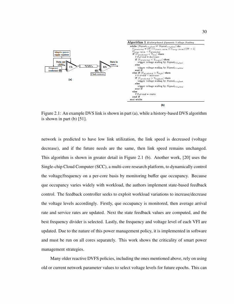
30

Figure 2.1: An example DVS link is shown in part (a), while a history-based DVS algorithmis shown in part (b) [51].

network is predicted to have low link utilization, the link speed is decreased (voltage

decrease), and if the future needs are the same, then link speed remains unchanged.

This algorithm is shown in greater detail in Figure 2.1 (b). Another work, [20] uses the

Single-chip Cloud Computer (SCC), a multi-core research platform, to dynamically control

the voltage/frequency on a per-core basis by monitoring buffer que occupancy. Because

que occupancy varies widely with workload, the authors implement state-based feedback

control. The feedback controller seeks to exploit workload variations to increase/decrease

the voltage levels accordingly. Firstly, que occupancy is monitored, then average arrival

rate and service rates are updated. Next the state feedback values are computed, and the

best frequency divider is selected. Lastly, the frequency and voltage level of each VFI are

updated. Due to the nature of this power management policy, it is implemented in software

and must be run on all cores separately. This work shows the criticality of smart power

management strategies.

Many older reactive DVFS policies, including the ones mentioned above, rely on using

old or current network parameter values to select voltage levels for future epochs. This can

31

Figure 2.2: A Threshold and PI controller Finite State Machine (FSM) are shown in (a),while a Greedy controller FSM is shown in (b) [30].

become problematic if future needs are not accurately represented, especially since voltage

levels are switched on the scale of 100s-1000s of cycles. If the optimal voltage level isn’t

selected, then the network will not have the opportunity to choose a new voltage level for

many cycles, meaning hundreds or thousands of cycles of excess power consumption or

lost performance. To ensure that the optimal voltage level is chosen, the voltage switching

logic must be supplied with an accurate estimate of future network needs to help combat

under/over estimation. If future network needs are over estimated, then the switching

logic will choose a voltage level that exceeds future needs, leading too little to no power

savings. If future network needs are under estimated, then the switching logic will choose a

voltage level that cannot meet future needs and performance will suffer. One work [31] uses

cache coherent protocols to determine future network states. This work differs from prior

reactionary techniques that focused on measuring current network parameters to estimate

future network needs because of the high prediction accuracy (87%) of cache-coherence

properties. In a cache-coherent NoC, traffic messages are defined by the coherence protocol

and must adhere to a strict set of communication rules. These protocols (ACKs, NACKs,

data requests, etc.) are sent from source to destination using end-to-end communication.

32

Figure 2.3: An example of simultaneous power, temperature, and performance manage-ment using Q-learning [52].

Because traffic messages in a cache-coherent NoC are regular and predictable, they are

used to better predict future network needs than typical parameters such as link/router

utilization, round-trip time, latency, or network slack. Due to this inherently exploitable

nature, the authors can rely on accurate predictions of future network demand which leads

to more optimal voltage level selection.

Newer methods have begun to incorporate machine learning techniques as they can

lead to highly accurate predictions of future network needs. RL algorithms can even

learn optimal control polices as data become available. One such work [22] uses online

learning based DVFS in a single-tasking and multi-tasking environment and compares

the potential energy savings of each. Another work [52] uses Q-learning based DVFS

to manage temperature, performance, and energy in a processor as shown in Figure 2.3.

33

2.2 LEAD Architecture

LEAD is built on a CMesh topology using a hierarchy of off-chip and on-chip voltage

regulators that allow the selection of multiple voltage modes as shown in Figure 2.4. Our

network consists of 16 routers, 64 cores, and 48 unidirectional links corresponding to a

more area/energy efficient network. We propose per router DVFS such that the router

as well as the outgoing links are scaled simultaneously to operate at the same mode of

operation. Each router consists of 8 input ports, 8 output ports, and 4 virtual channels

per port while each processor has an individual L1 cache and each router has an L2 cache

shared among the four cores connected to each router. DVFS is not applied to the cores,

LLC or other uncore components. When a packet is first generated, the packet is stored in

the input buffer. The output port is computed using XY dimension-order routing (DOR)

in the route computation (RC) stage of the router pipeline. After a virtual channel is

allocated, the head packet competes for the output channel in the switch allocation (SA)

stage. After successfully competing and being awarded the channel, the packet is sent

across the crossbar to the destination port in the switch traversal (ST) stage. The proposed

router microarchitecture is shown in Figure 2.5(a) [17].

2.2.1 Operating V/F Modes

Each LEAD model uses five modes of operation with voltage and frequency levels

similar to those proposed in previous work [31]. The supply voltage changes in 100

mV steps with proportional changes in clock frequency which allows decreased voltage

regulator framework complexity. The V/F pairs our models use include {0.8 V/1 GHz,

0.9 V/1.5 GHz, 1.0 V/1.8 GHz, 1.1 V/2 GHz and 1.2 V/2.25 GHz} which correspond to

modes 1-5 as shown in Figure 2.5(b). We carefully chose five modes to balance overhead

and energy savings because having a large number of V/F pairs leads to increased voltage

regulator overhead without the guarantee of increased energy savings, whereas too few

34

Figure 2.4: We apply LEAD to a CMesh with 16 routers and 64 cores. We use on chipvoltage regulators that can adjust the supply voltage between 0.8V and 1.2V, allowing usto apply DVFS to individual routers and their corresponding links [17]©2018 ACM.

modes will not allow the DVFS algorithm to exploit traffic load variation and save energy

at run-time [17]. Power-gating introduces several unique challenges (deadlocks, breakeven

time, loss in throughput) and while this chapter will not focus on power-gating, we have

implemented a power-gated version of LEAD which will be further discussed in Chapter

3.

2.3 DVFS Models and Implementation

In this portion of our work we focus on measuring the impact of different mode

selection models on dynamic energy savings and performance. In this chapter we propose

three machine learning based models; LEAD-τ, LEAD-∆, and LEAD-G. LEAD-G is based

35

Figure 2.5: The architecture as well as all additional units required for reactive or proactivemode selection are shown in (a). A simple voltage regulator setup that allows the selectionof voltage levels in the range of 0.8V to 1.2V for every router and its’ associated outgoinglinks is shown in (b) [17]©2018 ACM.

on an already proposed reactive model called Greedy. This Greedy model is presented in

[30] as an adaptation of a Greedy search method presented in earlier work [40]. Greedy

and LEAD-G are used strictly for comparative purposes. All three of these models do

not apply power-gating, but we will introduce an additional LEAD model that does apply

power-gating in chapter 3 [17].

Baseline: The baseline model always operates all routers in mode 5 (highest V/F

pair) and does not apply DVFS to the network. This model has the highest throughput and

lowest latency but has no dynamic energy savings [17]. We use this as our baseline because

it has the highest performance and we want to ensure energy savings with as little loss in

performance as possible.

LEAD-τ: This model starts each router in the lowest mode of operation, mode 1.

It then chooses the routers’ mode for the next epoch based on the predicted input buffer

36

utilization of the router for the next epoch. If the router’s buffers are predicted to be less

than 5% full, then the lowest mode is chosen. If the buffers are predicted to be between 5%

and 10% full, then mode 2 is chosen. If the buffers are predicted to be between 10% and

20% full, then the third mode is chosen. If the buffers are predicted to be between 20% and

25% full, then the router will operate in the fourth mode. Finally, if the buffers are predicted

to be greater than 25% full for the next epoch, then the router will operate in the highest

mode of operation, mode 5. For larger epoch sizes the thresholds are reduced for more

aggressive scaling to counter a larger theoretical maximum. This theoretical maximum is

calculated as a worst-case time variant sum over the duration of an epoch. For simplicity

sake we will show the thresholds as if they are all for epoch size of 100 cycles. The LEAD-

τ model assumes a voltage regulator scheme that allows the transition from any mode to

any mode in one cycle without the need to transition into adjacent modes [17]. While this

is not practical, real-valued switching delay is introduced into the models we present in

Chapter 3. This model emphasizes the importance of being able to select the optimal mode

at any given epoch versus other designs which are constrained to only being allowed to

transition into adjacent modes [17].

LEAD-∆: This model starts each router in the highest mode of operation, mode 5.

Every epoch routers’ transition one mode up/down based on the predicted change in input

buffer utilization between the current and future epochs. Mode transitions only occur if this

predicted change in buffer utilization falls within certain carefully selected criteria. These

criteria must ensure that small variations in network traffic over a short time span do not

govern mode selection over an entire epoch; however, it is critical that the router still be

able to adequately adapt to long-term changes in network traffic patterns. The buffers must

be predicted to increase by at least 6% of their maximum utilization over the next epoch to

warrant a mode transition into a higher mode, and they must be predicted to decrease by at

least 3% of their maximum utilization to warrant a mode transition into a lower mode for

37

the next epoch. We ensure dynamic energy savings by requiring the predicted change in

buffer utilization required to move down a voltage level be less than the change required to

move up. The LEAD-∆ model is used to compare the trade-offs associated with being able

to transition only into adjacent modes at every epoch and still assumes that each transition

takes one cycle. This model is more suited to gradual traffic changes where adjacent mode

transitions are optimal [17].

LEAD-G: This model (based on prior work [30], [40]) explores to find the mode that

minimizes a predicted future energythroughput2 . LEAD-G adds explorative logic and introduces

both dynamic energy and throughput into the label in the hopes of better balancing the

trade-off between the two. LEAD-G starts each router in the highest mode of operation

and in a downwards explorative direction. If the predicted change in energythroughput2 between the

current and future epoch is less than or equal to 0, then the router will move one mode

further in the current exploration direction (downward/upward). If the predicted change in

energythroughput2 is greater than 0, then the router is put into a hold phase. The hold phase lasts 2

epochs, a similar duration to prior work [30], and during the hold phase the router cannot

increase/decrease its’ voltage level. After the hold phase expires, the exploration direction

is flipped and the model begins to explore in the opposite direction until the predicted

energythroughput2 is greater than 0 again. This model seeks to minimize the predicted energy

throughput2 and

assumes that routers may only transition into adjacent modes. The logic behind all three

LEAD models is further explained in Figure 2.6 [17].

2.3.1 DVFS Implementation

As shown in Figure 2.5(a), LEAD uses four components per router in order to perform

reactive (non-ML) or proactive (ML) model selection. We have not mentioned how reactive

mode selection is done, but it is a simple process wherein each LEAD model uses current

values to govern mode selection instead of labels (predicted future values). This shall be

38

Figure 2.6: LEAD-τ uses a predicted input buffer utilization to select the optimal mode perepoch. LEAD-∆ uses a predicted change in input buffer utilization to move in the directionof the optimal mode per epoch. LEAD-G incorporates both energy and throughput into thelabel and moves up/down adjacent modes (based on exploration direction) such that energydivided by throughput is minimized [17]©2018 ACM.

further discussed in Chapter 4. The first additional router component is called Feature

Extract. It gathers local router/link features and supplies them to the Non-ML Model

unit. For reactive mode selection, the Non-ML Model unit takes key values supplied from

Feature Extract and selects the appropriate mode for the router and the router’s outgoing

links. For proactive mode selection, we require the addition of two new units. The

first component, Label, takes the features supplied by Feature Extract and applies Ridge

Regression to generate a corresponding label. This label is then supplied to the ML Model

unit to select the appropriate mode for the router and the outgoing links [17].

39

2.4 Machine Learning for DVFS

We use machine learning to train different Ridge Regression algorithms corresponding

to LEAD-τ, LEAD-∆, and LEAD-G. There are two arrays of values needed when using

regression, the first being the feature set and the second being the weight vector. Each

feature has a corresponding weight, a scalar factor representing the impact on predicting

the output. The Ridge Regression equation is shown below:

E(w) =12

N∑n=1

{y(xn,w) − tn}2 +

λ

2

M∑j=1

w2j (2.1)

Where,

xn = (xn1, xn2, ..., xnK) (2.2)

w = (w1,w2, ...,wi)T (2.3)

y(xn,w) =

K∑k=1

xn,k · wk (2.4)

In the Ridge Regression equation listed above, we minimize the sum of squared errors

between our predicted label y(xn,w) and the actual label tn. The feature vector xn

(containing K features) as well as the supplied labels tn are used to train the system offline

such that a corresponding weight vector w (also of size i) is created. During tuning, different

values of λ are tried for the equation λ2

∑Mj=1 w2

j until the best fitting solution for the training

data is found. This validation phase is important as it helps reduce model complexity

and combat over-fitting. We used a total of 14 different trace files; 6 for training, 3 for

validation, and 5 for testing [17].

Feature Set: The feature set is directly related to prediction accuracy and overhead

cost. The feature set must be kept as small as possible because every new feature

increases computational overhead during label generation. Features must also be carefully

chosen such that accurate predictions of future network needs can be gleaned from them.

Our feature set for this work is composed of 39 network parameters (buffer utilization,

40

incoming/outgoing link utilization per direction, request/response packets, etc.) as well as

a label local to each of the 16 routers [17]. The full LEAD feature set is shown in Chapter

4, while a reduced feature set obtained after extensive feature engineering and testing will

be presented in Chapter 3.

Label: A reactive version of each LEAD model is used to govern mode selection for

all training and validation trace files so that features and labels can be extracted. This data is

then used to train/validate each LEAD model. While the same features are used to train all

LEAD models, the label supplied for training is unique to each LEAD model. Therefore,

after training/validation each LEAD model will be composed of a uniquely trained set of

weights. The label for LEAD-τ is the future input buffer utilization of the router for the

next epoch. The label for LEAD-∆ is the difference between the routers’ current and future

buffer utilization. The label for LEAD-G is the difference between the routers’ current and

future energythroughput2 . These labels are supplied along with the corresponding features to train

and validate all ML algorithms offline [17].

ML Overhead: A trained linear regression algorithm uses a series of additions and

multiplies to calculate a label; thus, the overhead cost can be simplified to the timing,

power, and area cost required to execute a set number of additions and multiplies. The

energy cost of a single 16 bit floating point add is estimated to be 0.4 pJ and the area cost is

1360 um2 [32]. The energy cost of a multiply is estimated to be 1.1 pJ and the area cost is

1640 um2 [32]. The total energy overhead cost is 58.1 pJ (considering two-stage multiplies

followed by an addition). The total area overhead cost is 0.12 mm2, and the total timing

cost is 3-4 cycles [17]. We use larger epoch sizes of 500 cycles and 1000 cycles to ensure

that such overhead costs are kept relatively small as labels only need to be calculated once

per epoch.

41

3 DozzNoC: Combination ofML based DVFS and

Power-Gating for NoC

This chapter focuses on the introduction of DozzNoC, a power-gated LEAD model.

DozzNoC enables energy proportional computing by applying both power-gating and

DVFS to network routers and links. DozzNoC applies power-gating at times of network

idleness and DVFS at times of low-high network traffic; this will be discussed in greater

detail in section 2.2. While previously introduced in section 1.4, a more detailed discussion

of select prior power-gated techniques will be presented in the first section of this

chapter. The second section will focus on our proposed DozzNoC architecture and network

topology, followed by an in-depth explanation of the various DozzNoC states, as well as

how states and operational modes are selected. The last section of this chapter will detail

how we have applied machine learning to DozzNoC, heavily drawing from our LEAD

models. We will also detail the reduced feature set, label, and reduced ML overhead.

3.1 Related Works

Much prior PG research has focused on the application of runtime power-gating to

both the core and various uncore components as well as the NoC. Power-gating is used to

completely power off unused or lightly used cores or other network components. Successful

power-gating techniques can drastically reduce leakage power, making them critical for

energy proportional computing. Most designs that apply power-gating to the NoC assume

a single network. If a downstream router or link is power-gated, network connectivity will

be lost. Typically, this scenario results in performance loss and introduces the risk of dead-

locks and live-locks. Therefore, preventative measures such as data re-routing or early

wake-up must be taken.

42

Other research has focused on the benefits and trade-offs associated with applying

power-gating at various time granularities. Coarse-grain power-gating methods that use

large re-configuration windows of 10K cycles or more have several major drawbacks. The

first drawback comes from cutting network connectivity for large periods of time, which

can result in massive performance loss if counter measures such as bypass paths or packet

re-routing are not implemented. The second drawback comes from the inability to exploit

small periods of router idleness of 10-100 cycles that are common across real traffic patterns

and applications. Both problems are solved with smaller re-configuration windows. Such

techniques employ header transistors with high threshold voltage that cut power when the

sleep signal is asserted. Fine-grain power-gating can achieve up to 10x reduction in leakage

power, therefore I will focus on newer research that use smaller re-configuration windows.

One such work seeks to avoid loss of connectivity by breaking the network up into

several smaller but fully connected networks in a Multi-NoC architecture [19]. This

Multi-NoC design is built on a 256-core CMesh with 8 memory controllers. This design

partitions wires, buffers, and other network components into several subnetworks built

from proportionally smaller components. This Multi-NoC concept is visualized in Figure

3.1. Figure 3.1 also highlights the differences between a Single-NoC and a Multi-NoC

composed of four subnetworks. If link width in a Single-NoC was 512 bits, it would

equal 128 bits in a Multi-NoC. This same concept is also applied to the router and other

network components. If all four subnetworks are active, then total bandwidth in the Multi-

NoC would remain unchanged from the original larger Single-NoC. This allows Catnap

to power-gate entire subnetworks proportional to network demand without loss in network

connectivity. Catnap uses a unique subnet-selection policy to determine what subnetwork

new packets are injected into, and a unique power-gating policy to determine when a

subnetwork should be switched on/off. Catnap routers can be in three different power

states: active, sleep, and wake-up. In the active state, routes are on and operational and can

43

Figure 3.1: The difference in network component sizes between a Single-NoC and a Multi-NoC [19].

be used to send/receive data. In the sleep state, routers are powered off and cannot be used.

In the wake-up state, local voltage levels are being charged up to Vdd and the router cannot

be used until the wake-up delay has been met, which the authors estimate to be 10 cycles.

There is also the energy cost to wake-up a powered off router, which was estimated to be

around 12 cycles worth of leakage energy. Catnap demonstrates that a power-gated Multi-

NoC design can consume about 44% less power than a bandwidth proportional Single-NoC

for a minimal 5% loss in performance.

Normally a router cannot be used to send/receive or forward data unless it is powered

on, however one work seeks to decouple the node’s ability to send/receive packets from

the power state of the router [11]. This is accomplished by providing separate wake-

up avoidance decoupling bypass paths, alleviating the need for packets to wait until the

router has been woken up. Packets have the option to choose between normal paths and

bypass paths if routers are power-gated. This approach allows the network interface to

44

Figure 3.2: The NoRD network bypass ring is shown in (a), the router bypass datapath isshown in (b), and the network interface datapath is shown in (c) [11].

forward packets directly into specific input ports of the router via bypass paths, forming

a fully connected unidirectional ring. The network level bypass channel, the additional

router level bypass path, and the network interface bypass path are shown in Figure 3.2(a-

c) respectively. NoRD operates while trying to fulfill two key objectives. The first objective

is to maximize net energy savings which is done by maximizing the amount of router off

time. NoRD must ensure that during fragmented idle periods packets have a bypass path

around powered off routers, ensuring they are not woken prematurely. The second objective

is to minimize performance loss, which is done by ensuring that wake-up delay is reduced

or hidden entirely. This can be accomplished by routing around powered off routers. If the

wake-up delay is not properly hidden, it can compound across multiple hops. This work

estimates typical wake-up delay to range from 10-20 cycles depending on clock frequency.

The authors also estimate the break-even time to be approximately 10 cycles, slightly less

than Catnap’s estimated 12 cycles. However, these delays and break-even times are largely

hardware dependent. NoRD shows that by decoupling the node and router, static energy

can be reduced by an additional 29.9% over traditional power-gating techniques that fail to

exploit periods of fragmented traffic.

45

Another work focuses on minimizing the performance loss incurred from wake-up

delays by sending wake-up signals to downstream routers [13]. The authors of this work

accomplish that goal using two key mechanisms. The first ensures that power control

signals utilize existing network slack to wake up initial routers in the packets path. The

second mechanism ensures that wake up signals stay sufficiently far ahead of the packet

to “punch through” blocked routers. Router blocking occurs when a packet arrives at a

router that is powered off and must wait for it to be turned on to switch across it. As

previously mentioned, this delay can become compounding if multiple routers are powered

off in the packets path resulting in massive performance loss. However, some of this delay

can be hidden simply by sending a wake-up signal to downstream routers once the route is

calculated. Power Punch demonstrates how early wake up detection enables power-gated

schemes to save up to 83% of router static energy with minimal impact on execution time.

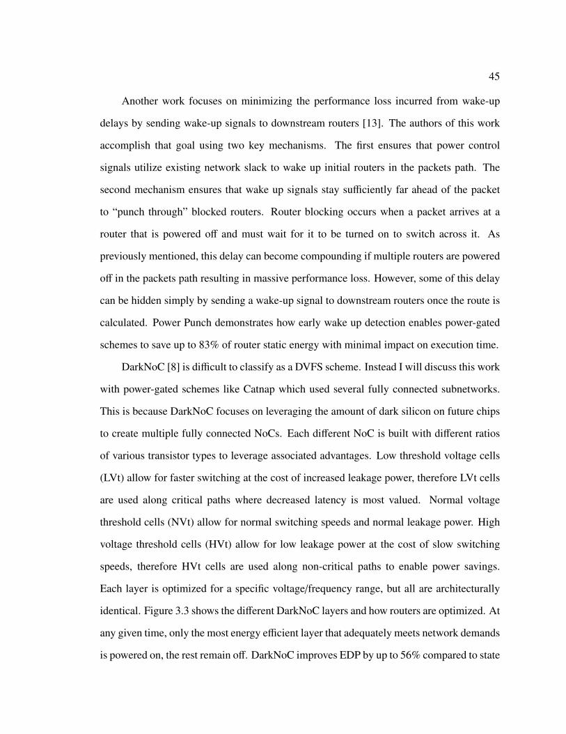
DarkNoC [8] is difficult to classify as a DVFS scheme. Instead I will discuss this work

with power-gated schemes like Catnap which used several fully connected subnetworks.

This is because DarkNoC focuses on leveraging the amount of dark silicon on future chips

to create multiple fully connected NoCs. Each different NoC is built with different ratios

of various transistor types to leverage associated advantages. Low threshold voltage cells

(LVt) allow for faster switching at the cost of increased leakage power, therefore LVt cells

are used along critical paths where decreased latency is most valued. Normal voltage

threshold cells (NVt) allow for normal switching speeds and normal leakage power. High

voltage threshold cells (HVt) allow for low leakage power at the cost of slow switching

speeds, therefore HVt cells are used along non-critical paths to enable power savings.

Each layer is optimized for a specific voltage/frequency range, but all are architecturally

identical. Figure 3.3 shows the different DarkNoC layers and how routers are optimized. At

any given time, only the most energy efficient layer that adequately meets network demands

is powered on, the rest remain off. DarkNoC improves EDP by up to 56% compared to state

46

Figure 3.3: Four seperate DarkNoC layers are shown in (a), a single DarkNoC layer isshown in (b), and DarkNoC routers are shown in (c) [8].

of the art DVFS techniques, however due to the nature of this design it would require four

fully connected NoCs, potentially quadrupling the area overhead of the NoC.

3.2 DozzNoC Architecture

DozzNoC improves upon LEAD with enough versatility to be applicable to multiple

network topologies. We specifically apply DozzNoC to both a CMesh and a mesh network

topology unlike LEAD which was only applied to a CMesh [16]. When applying DozzNoC

to a CMesh we use a 4 × 4 NoC with a concentration factor of 4. When applying DozzNoC

to a mesh we use an 8 × 8 network with 64 cores. We can easily switch between other

network topologies and scale to increased numbers of routers because we use only local

router features to select voltage levels. Using only local router features is critical because

we eliminate the need for global co-ordination. This means adding a new router is as simple

as adding another voltage regulator and will incur minimal amounts of extra computational

overhead. The difference between applying DozzNoC to a mesh and CMesh network can

be seen in Figure 3.4(a,b). When applying DozzNoC to a CMesh network, we use larger

routers with 8 input ports, 8 output ports, and 4 virtual channels per port. When applying

47

Figure 3.4: We apply DozzNoC to both a CMesh in (a), as well as a mesh in (b). The routermicroarchitecture for a mesh topology is shown in (c) [16].

DozzNoC to a mesh network, we use smaller routers with 5 input ports, 5 output ports,

and 4 virtual channels per port. Processor count remains unchanged between topologies

and each core has a separate L1 cache, however, in a CMesh the L2 cache is shared among

cores. The router microarchitecture for DozzNoC remains unchanged from LEAD. Newly

generated packets sit in the input buffers of the routers. This location corresponds to the

packets’ injection source. Next the output port is computed using look-ahead routing in

the route computation stage. We then use XY dimension order routing to select the output

ports. We also use this information to ensure that downstream routers are not allowed to

be powered-off, and if they are off, to wake them up for a partially non-blocking power-

gated scheme. Naturally it would be more difficult to design a partially non-blocking

power-gated scheme if we did not use XY routing, but it is still achievable if downstream

routers can be determined and woken up in advance. Next, a virtual channel is allocated

to the packet and it competes for the output channel. Lastly, the packet is sent across the

crossbar and into the destination port after a successful switch traversal [16]. Our proposed

router microarchitecture does not really change from LEAD, therefore we will not replicate

previously presented material. However, we have removed one redundant component. The

48

new DozzNoC router microarchitecture is shown in Figure 3.4(c), while Figure 3.4(a)

shows DozzNoC being applied to a CMesh and Figure 3.4(b) shows DozzNoC being

applied to a mesh.

3.2.1 Operational States

Routers and links under DozzNoC are given three states of operation as shown in

Figure 3.5. These three states include an inactive state, an active state, and a wakeup state.

While these states appear to be similar to the states one would observe from a normal

power-gated scheme, the active state is unique [16]. All wake-up and switching latencies

are estimated using equivalent capacitance of a router and its’ outgoing links, however the

voltage regulator design as well as the specific values for voltage switching and wake-up

delay were created and evaluated by another team of researchers. While the switching and

wake-up delays are based on real values, they will not be discussed in this thesis, nor will

the voltage regulator design.

Inactive State: In this state, the power supply to an individual router and its’ outgoing

links is reduced to 0 V , thus the router and associated links are completely switched off.

While in an inactive state, the router and its’ outgoing links consume no power. However,

inactive components may not be used to send/receive packets and cannot be used to hop

packets across them. The router can transition from an active state to an inactive state in a

single cycle, but it must satisfy specific conditions before it is allowed to switch off. For

this work we ensure that the routers’ buffers have been empty for several consecutive cycles

and that it is not a downstream router before we allow the router to be switched off [16].

Wakeup State: A router that is in the process of transitioning from an inactive state to

an active state goes into a wakeup state. While in the wakeup state, the router consumes

the same amount of power as if it were on as it is supplied with one of 5 various Vdds.

However, components that are in this state may not be used to send/receive packets and it

49

Figure 3.5: Our version of Power Punch acts as a baseline and is shown in (a). LEAD-τ hasonly one state, the active state; however active routers may operate at one of five differentvoltage levels (b). DozzNoC has three states and when a router is active it may operate atone of five different voltage levels as shown in (c) [16].

may not be used to hop packets across them until the wake-up delay has been satisfied. This

is similar to prior work that also called this a ”wake-up” state [19]. A router can transition

from an inactive state to a wakeup state in a single cycle, but the router must wait in the

wakeup state for a set amount of cycles before it can be considered fully on and functional.

In a power delivery system this is called the wake-up time, and it is defined as the interval

from the instant of a voltage change until the local voltage level settles to meet the supply

voltage level [16].

Active State: A router that is in an active state can operate at one of five different

voltage levels. These different V/F pairs are referred to as various modes of operation in

which the supply voltage and clock frequency are proportionally increased/decreased. The

V/F pairs our DozzNoC model uses in this work are {0.8 V/1 GHz, 0.9 V/1.5 GHz, 1.0

V/1.8 GHz, 1.1 V/2 GHz and 1.2 V/2.25 GHz} which correspond to being in the active

state in modes 3-7. We start the numbering at mode 3 because we consider mode 1 to be

the inactive state and mode 2 to be the wakeup state. These V/F pairs are similar to those

used in other works [17, 31]. A key difference in this portion of our work is that we use real

valued switching delays obtained from a unique SIMO voltage regulator design supplied

50

Figure 3.6: DozzNoC mode selection is shown in (a), while LEAD-τ mode selection isshown in (b) [16].

by other researchers in [16]. We chose not to add/remove modes for several reasons. First,

we wanted to maintain a fair comparison against prior work that used a similar number of

V/F pairs. Secondly, we did not wish to add unnecessary design complexity [16].

3.3 Power-Gated DVFS Models

This research focuses on combining the static power savings of power-gating with the

dynamic energy savings of DVFS. To that end, we propose two machine learning models

built on a power-gated framework that use supervised learning to train the regression

algorithm. These two algorithms correspond to DozzNoC and ML+TURBO. We also

compare to our best performing LEAD model from prior work that also used machine

learning and DVFS, LEAD-τ. All three machine learning models use the same threshold

based DVFS mode selection logic. This logic looks at the predicted future buffer utilization

and compares it to a theoretical maximum to determine what mode should be selected for

the next epoch. The state transition logic for all three ML models is shown in Figure

51

3.6. DozzNoC and ML+TURBO use the state selection logic from part a, while LEAD-

τ will never transition out of the active state. When the router is in the active state, all

three comparative ML models use the logic in part b to select the optimal voltage mode.

ML+TURBO was added to see the impact on static power and dynamic energy when the

highest mode is chosen instead of a lower predicted mode [16].

Baseline: The baseline model starts with all routers operating in the active state at the

highest voltage level, mode 7. The Baseline does not allow the transition of a router into

any other state. Therefore, all routers are always active and always operate in mode 7. This

model will always have the highest throughput and the lowest latency as it incurs no router

wake-up delay and no voltage level switching delay. However, the baseline offers no static

power savings and no dynamic energy savings and is mostly used as an upper bound on

performance and power cost [16].

Power Punch (PG): The Power Punch model is based on prior work from which the

name was created [13]. This model is not an exact replica of Power Punch, rather it behaves

similarly in that look-ahead routing is used to wake-up downstream routers and minimize

the impact of router blocking. Therefore, it is used for comparative purposes against a

state-of-the-art power-gating technique. This model operates routers individually in one of

three states. Either a router is inactive, waking up, or active. If the router is inactive, then

it consumes no power but cannot be used to send/receive packets. If a router is waking

up, it consumes the same amount of power as if it was active, but it cannot be used to

send/receive packets. Finally, if a router is active, then it will operate at the highest mode

of operation, mode 7. For a router to transition from an active state to an inactive state,

it must be idle for at least T-Idle consecutive cycles. A router is considered idle only if

its’ input buffers are empty and it is not a downstream router. This secondary condition

was developed to make this model as non-blocking in nature as possible so that a fairer

comparison to Power Punch can be made. We use XY look-ahead DOR routing, which

52

allows us to easily know the next router in a packets path so that downstream routers can

be secured. When a router is in a secured state, it cannot be switched off. If it is currently

off, it will immediately transition into a wakeup state where it will stay until the wake-up

delay has been met. The main purpose of this model is to compare the static power savings

of a state-of-the-art power-gating technique against a design that combines power-gating

and DVFS [16].

DozzNoC (ML+PG+DVFS): The DozzNoC design uses the same underlying

partially non-blocking power-gated design proposed earlier wherein all routers may be in

one of three states. In the inactive state, a router consumes no power but cannot be used

to send/receive packets. Transitioning to an inactive state takes a single cycle, and in order

to transition to an inactive state the router must first be in an active state and idle for more

than T-Idle consecutive cycles. The second state is the wakeup state. A router transitions

to a wakeup state when it is off and needs to be woken up. A router in the wakeup state

cannot be used to send/receive packets until the wake-up delay has been met. The length of

the wakeup state depends on the voltage level of the active state and is based on real values

presented in prior work [16]. The final state is the active state. A router that is in an active

state may send/receive packets and operate like normal. However, the key difference is that

DozzNoC uses predictive machine learning techniques to determine the optimal voltage

level for a router that is in an active state. This means that DozzNoC dynamically adjusts

the supply voltage to select the optimal active state operational mode. In order to do this,

we predict future input buffer utilization of a router and then compare this to the theoretical

maximum utilization to determine the optimal voltage level. This optimal voltage level

must meet network performance demands while still ensuring dynamic energy savings.

This DVFS design relies on aggressive voltage scaling that minimizes potential loss in

throughput. For epoch size of 100 cycles, if we predict the buffers to be less than 5% of

the maximum over the next epoch, we select the lowest voltage level for the active state to

53

Figure 3.7: A walkthrough example showing the difference in active state mode selectionacross two epochs for a dummy network [16].

operate at, mode 3. Mode 3 is considered the lowest mode of operation because mode 1

corresponds to the inactive state and mode 2 corresponds to the wakeup state. If the buffers

are predicted to be between 5% and 10% of the maximum we select mode 4, if the buffers

are predicted to be between 10% and 20% we select mode 5, if the buffers are between 20%

and 25% we select mode 6, and finally if the buffers are predicted to be more than 25% full

we select mode 7. These thresholds are slightly different at higher epoch sizes as they need

to be more aggressive to counteract a higher theoretical maximum [16].

In Figure 3.7 we show a walk-through example detailing how routers and links in

a dummy network would transition between different states on a per cycle basis. We

54

also show how the optimal active state voltage level is updated every epoch. R-Idle is

the number of consecutive cycles that a router has been idle, while R-Wakeup is used to

measure the number of cycles a router has spent in the wakeup state. For example, if in the

first epoch (Ek) DozzNoC predicts that the input buffers will be greater than 25% full for the

next epoch, then it will subsequently determine that the optimal active mode of operation

is the highest mode. This is highlighted with router 1 operating at the highest mode until

it is turned off, and router 2 waking up into the highest mode after the wake-up delay

is satisfied (RWakeup = 0). Router idleness (RIdle) along with number of cycles a router has

been waking up (RWakeup) are measured every cycle. A router will only switch off if a router

has been idle for several consecutive cycles (T-Idle) meaning the buffers are empty and it

is not a downstream router. Once a router is off, it must wait several cycles corresponding

to the wake-up delay before it is useable (T-Wakeup). This delay is kept track of by setting

RWakeup = TWakeup and subtracting one from Rwakeup every cycle. Once the router is finished

waking up (RWakeup = 0) we may use the router. If at the next epoch Ek+1 DozzNoC predicts

that the input buffers will be less than 5% full for the next epoch, then it will subsequently

determine that the optimal active mode of operation is the lowest mode. Thus router 1 will

now operate in the lowest mode when active and router 2 will operate in the lowest mode

after it successfully transitions from the wakeup state to the active state. When the router

has been idle for T-Idle consecutive cycles it is turned off, as can be observed by router

1. When a router is no longer considered idle (RIdle = 0), it transitions from the inactive

state to the wakeup state as shown by router 3. While this example network has only four

routers, the actual network will have 16 routers for a CMesh and 64 routers for a mesh.

The three states, inactive, wakeup and active will remain the same as the dummy network.

However, in this example a router in the active state has only three modes of operation, low,

medium and high while the real network has five operational modes. Also, for simplicity,

55

all routers in the dummy network have the same active mode of operation, while in the real

network each individual router selects operational modes based on local router labels [16].

LEAD-τ (ML+DVFS): LEAD-τ [17] is used for comparative purposes so that

throughput loss and dynamic energy savings of DozzNoC can be compared to prior work

that only applied machine learning-based DVFS to the NoC. While using this model, the

router can only be in the active state and may never transition to an inactive or wakeup state.

While in the active state LEAD-τ uses the same mode selection logic as DozzNoC where

future input buffer utilization is predicted, and an optimal active voltage level is selected.

This model may transition from any voltage level to any other voltage level within the range

of 0.8V to 1.2V. The main purpose for including this model is to compare how a stand-alone

machine learning DVFS design performs against a machine learning design that has DVFS

and power-gating [16].

ML+TURBO: This model seeks to apply power-gating and DVFS to the NoC in a

similar fashion to DozzNoC. It uses the same three states of operation as DozzNoC; the

inactive state, the wakeup state, and the active state. When a router and its’ links are active,

a prediction of the future input buffer utilization is used to govern the voltage level. The

key difference between this model and DozzNoC is that every three times we predict that a

router should be at any active mode other than mode 3 or mode 7, we instead select mode

7. The key goal of this model is to improve throughput and static power savings at the cost

of dynamic energy since we opt for the highest operational mode even if we predict a lower

mode sufficient to meet network demand [16].

3.4 Machine Learning for PG-DVFS

Machine Learning enables us to use proactive mode selection techniques for DozzNoC

and all comparative models. This allows DozzNoC to use ML techniques to select

operating voltage levels while in the active state. The underlying ML equations have not

56

changed between LEAD and DozzNoC. We use the same Ridge Regression optimization

formulation as in Section 2.4, and the feature vector and weight vector are trained and

validated in the same way. The major difference for DozzNoC is that extensive feature

engineering allows us to reduce the number of features to only 5.

Feature Set: The feature set is carefully crafted such that prediction accuracy is

maximized while overhead is kept to a minimum. This is accomplished by selecting local

router features that give the greatest insight into network performance while also keeping

the relative number of features small. For DozzNoC we determined the features that were

most relevant to accurate label prediction exhaustively as is shown in 4.5. This will be

further explained in the results section. We found that it is possible to reduce the number

of features (starting with the same 41 features proposed in prior work) without having a

significant impact on the overall performance, which is shown in 4.6. Each additional

feature equates to more run-time computational overhead because the number of additions

and multiplications necessary to generate the label increases. The original feature set

proposed in [17] contained 41 features in total as well as a label, however we have reduced

this to only five critical features. These five features are listed in detail in Table 3.1 [16].

Table 3.1: DozzNoC’s Reduced Feature Set [16]

Feature Set:

Feature 1: Array of 1’s

Feature 2: Requests Sent by All Cores

Feature 3: Requests Received by All Cores

Feature 4: Router Total Off Time

Feature 5: Current Input Buffer Utilization

Label: Future Input Buffer Utilization

57

Label: Label generation for DozzNoC remains unchanged from LEAD, however,

LEAD used 40 features, while DozzNoC uses only 5. Like LEAD, DozzNoC and all

comparative models are trained offline and are ready to use at test time [16].

Machine Learning Overhead: After a model has been trained, the weight vector is

exported to the network simulator where it can be used to select voltage levels when routers

are active. The additional overhead incurred from machine learning can be broken down

into the timing, area, and energy cost to execute a series of additions and multiplications

as this is how a label is calculated. Each feature is multiplied by its equivalent weight and

then the results are summed to generate a label. Prior work [32] has already estimated the

cost to do these operations and they do not change from LEAD ML overhead. Prior work

that used 41 features calculated the total energy overhead cost to be 61.1pJ, the total area

overhead cost to be 0.122 mm2, and the total timing cost to be 3-4 cycles. We will show

in Chapter 4 that the feature set can be reduced to 5 features without causing a significant

impact on model performance. Therefore, the overhead to generate a label for DozzNoC

and all comparative models can be reduced to only 5 multiplications and 4 additions. This

equates to a total energy overhead cost of 7.1pJ, a total area overhead cost of 0.013 mm2,

and a total timing cost of 3-4 cycles per router. Our epoch size is 500 cycles, with label

generation occurring on a per router basis once per epoch. However, if the additional

energy overhead were too large, it could be further reduced by increasing the size of the

epoch. If the area overhead was too large, it could be reduced by forcing routers to share

computational resources, which would increase the timing overhead proportional to the

amount of shared resources [16].

58

4 Performance Evaluation

4.1 LEAD Simulation Methodology

In this chapter we evaluate the static power and dynamic energy savings as well as

the performance trade-offs for our various proposed LEAD (LEAD-τ, LEAD-∆, LEAD-

G) and DozzNoC (DozzNoC, LEAD-τ, ML+TURBO) models. For fair comparison,

we specifically apply all LEAD models to a 4×4 CMesh topology with 64 cores. We

evaluate all LEAD models across 13 different real traffic traces gathered using Multi2sim.

Multi2sim [58] is a full system simulator that uses CPU benchmarks from PARSEC 2.1

[5] and SPLASH2 [61] in order to generate cycle accurate traces. These traces are used as

input for our in-house network simulator, where reactive versions of each LEAD model are

run such that features and labels can be extracted. The 13 different traces used to train and

validate each LEAD model are shown in Table 4.1.

Table 4.1: LEAD Benchmarks

Training Validation Testing

Barnes Raytrace Lu (non-contiguous)

Blackscholes Swaptions Lu (contiguous)

Bodytrack Ferret Radix

Dedup Fluidanimate

FFT Canneal

Ocean

The goal of using trace files generated with PARSEC 2.1 and SPLASH2 benchmarks

for these simulations is to evaluate the throughput, latency, and dynamic energy of various

machine learning enhanced voltage switching models across real traffic patterns. LEAD is

implemented in our in-house network simulator; therefore, each line of the trace file need

59

only consist of relevant packet data. This data includes packet injection source, packet

destination, packet type, and injection cycle. Packet source and destination information

must be known to calculate the route. It is also important that we know the packet type

(request or response) because only requests are used as inputs. Our network simulator

will automatically generate a response packet once a request has been received. It is also

crucial that we know the injection time since our results must be cycle accurate. Specific

Multi2sim parameters used to gather trace files are shown in Table 4.2.

Table 4.2: Multi2sim Parameters

Cores 64

Routers 16

Concentration Factor 4

L1/L2 Coherence Protocol MOESI

Private L1/L2 Yes

Private LLC No

L1 Instruction Cache Size (kB) 32

L1 Data Cache Size (kB) 64

L2 Cache Size (kB) 256

L3 Cache Size (MB) 8

Main Memory Size (GB) 16

We used DSENT [57] to model routers and links so that the resulting dynamic power

results could be converted into energy per hop. The energy per hop is gathered for all 5

different V/F pairs at a 22 nm technology node assuming a 128-bit flit width [17]. The

total dynamic energy is calculated as the cost to send a specific number of packets through

the network, where every hop is recorded and the cost per hop is known. Each entry

in a trace file contains a single packets injection information, therefore total packets sent

60

equal total requests in the trace file. Naturally the number of requests may vary slightly

between trace files, however, the number of packets sent per trace is still constant across

all LEAD models. The energy per packet is calculated as the cost to traverse a router and

an outgoing link. Routers and links may operate at one of five different operating voltages

corresponding to modes 1-5, thus energy per hop will change accordingly. This energy

cost is listed starting from lowest mode to highest mode: {25 pJ/packet, 32 pJ/packet, 39

pJ/packet, 47 pJ/packet, 57 pJ/packet} [17]. The voltage and frequency of each mode as

well as packet traversal energy is shown in table 4.3.

Table 4.3: Dynamic Energy Per Hop (Modes 1-5) [17]©2018 ACM

Mode 1 0.8V 1.0 Ghz 25 pJ/packet

Mode 2 0.9V 1.5 Ghz 32 pJ/packet

Mode 3 1.0V 1.8 Ghz 39 pJ/packet

Mode 4 1.1V 2.0 Ghz 47 pJ/packet

Mode 5 1.2V 2.25 Ghz 57 pJ/packet

4.1.1 LEAD Model Variants

For the LEAD-τ model, we needed to determine the ideal input buffer utilization

thresholds for switching between modes. To determine these ideal mode transition

thresholds, we conducted an exhaustive study. Figure 4.1 shows a small set of our threshold

studies on a single trace file. Each model variant’s name (shown on the x-axis) consists

of 4 values that correspond to the mode transition thresholds. For example, 5/10/20/25

implies a transition from mode 1 to mode 2 when buffer utilization exceeds 5%, from

mode 2 to mode 3 when the buffer utilization exceeds 10%, from mode 3 to mode 4 when

buffer utilization exceeds 20%, and finally a transition to mode 5 when buffer utilization

is above 25%. From Figure 4.1, we observe that the set of thresholds that lead to the

61

Figure 4.1: The throughput loss and dynamic energy savings across multiple LEAD-τvariants with an epoch size of 500 cycles [17]©2018 ACM.

best performance (lowest throughput loss and maximum energy savings) was 5/10/20/25

which yielded 15.51% energy savings while showing 5.35% throughput loss across a single

training trace file. Therefore, we use 5/10/20/25 threshold values for our LEAD-τ model

[17]. For the LEAD-∆ and LEAD-G models, similar testing occurred. LEAD-∆ model

variants changed the thresholds needed to transition up or down a voltage level, while

LEAD-G model variants changed the number of hold cycles before the model could change

explorative directions. Only the best performing models are shown in the results section.

4.1.2 LEAD Mode Breakdown

In Figure 4.2 we show the amount of time spent in each of the five different modes

across all five test applications for the best performing LEAD models. Every epoch the

routers’ current voltage level is recorded, and one of five various counters is incremented

corresponding to the routers’ voltage level. This is done for all 16 routers every epoch

so that total network time spent in each mode can be calculated. LEAD-τ has the unique

ability to switch from any-to-any mode, which allows it to avoid mode 4 altogether. We

can observe how LEAD-τ routers spend most of their time in the highest mode of operation

but can switch into lower modes to exploit idle traffic patterns. This ensures that LEAD-τ

62

Figure 4.2: The time routers and links spent in each mode for all LEAD models across alltest traces [17]©2018 ACM.

minimizes loss in throughput while maximizing energy savings. Both LEAD-∆ and LEAD-

G show significant amounts of time spent in the lower modes 2 and 1 respectively. However,

LEAD-∆ routers have a very even distribution of time spent in each of the five different

mode of operation, corresponding to the gradually changing nature of the model. LEAD-G

routers show the exact opposite behavior of LEADτ wherein they wish to stay in the lowest

mode of operation as much as possible to maximize energy savings. The LEAD-G model

does not conserve performance at high network load. All three models and their behaviors

will be discussed further in the following sections.

4.2 LEAD ML Simulation Methodology

Each LEAD model is trained using Ridge Regression, a machine learning algorithm

that minimizes the sum of squared errors and adds a regularization term. We must gather

training and validation data as well as test data to evaluate model performance. LEAD uses

supervised machine learning, thus both features and corresponding labels must be gathered

for training and validation. Labels are unique to each of the three different LEAD models

63

and will be discussed in greater detail in the following section. To gather training data, a

reactive version of each LEAD model is used to govern mode selection. Then, at every

epoch (100-1000 cycles) features as well as the previous epochs corresponding label are

exported to a text file for every router.

From Table 4.1, we observe that six trace files are used to gather features and target

labels, three are used to validate the trained models, and the remaining five are used at

test time to evaluate model generalization. This process must be repeated for each LEAD

model as each will have a unique reactive version used to gather training/validation data,

and each will have unique target label. This results in each LEAD model having a unique

set of trained weights which are exported for use during test time. It is important that we

tune the lambda hyper-parameter during the validation phase as it controls the amount of L2

regularization used to combat over-fitting. If the model over-fits, it will generalize poorly.

This means the model will perform very well on the training data but will perform poorly

at test time. Model training and tuning occurs in Matlab where we have implemented

our Ridge Regression algorithm. After this phase concludes, trained weights are exported

back to our in-house network simulator where they are used on test traces to predict router

specific target labels every epoch. These labels are used to govern mode selection and

enable proactive voltage switching. The five trace files used at test time are completely

untouched during training/validation. Seeing them in advance would be equivalent to

cheating, thus generalization performance could not be accurately measured.

4.2.1 LEAD Feature Engineering

The process of feature engineering involves selecting specific network parameters to

use as inputs for label generation while keeping overhead to a minimum. If the label is

the future state of the network, then features should contain relevant network information

that will help predict this future state. For example, the label for LEAD-τ is input buffer

64

utilization over the next epoch, therefore the most critical feature is the input buffer

utilization over the current epoch. Knowing the current value of a parameter helps pattern

recognition software predict the future value of that parameter immensely. We use a total

of 39 features ranging from requests sent and received on all directions, responses sent and

received on all directions, incoming and outgoing link utilization in all directions, current

input buffer utilization, current change in input buffer utilization, current slack, and current

voltage level.

The first feature is an array of 1’s, this is used for weight normalization. The

next several features are Requests/Responses sent and received on every direction.

These features are important because they provide the algorithm with useful direction

specific traffic insights. This adds directional traffic flow information to label generation.

Incoming/Outgoing link utilization help determine whether the performance needs of the

network are increasing or decreasing. These features are critical to determine whether

router modes should be increased or decreased to meet such changing needs. However, the

most critical feature for predicting future input buffer utilization, is knowing the current

input buffer utilization. Therefore, feature 36 is mainly added to improve performance

of the LEAD-τ model. Likewise, knowing the current change in input buffer utilization

between the last and current epoch is very helpful when trying to predict this change for

the next epoch. Therefore, feature 37 was added largely to help performance of the LEAD-

∆ model, however feature 36 is still important for this label as well. Similarly, feature

38 was added to help label generation of the LEAD-G model. The feature set does not

change between LEAD models, only the corresponding label changes. Therefore, we tried

to select enough key features such that each of the three various labels can be accurately

generated at test time using the same feature set. Each feature contains only local router

information with the full list of features given in two separate Tables 4.4 and 4.5. The

feature set is split into two different tables because of page size limitations. It is crucial

65

Table 4.4: Full LEAD Feature Set

LEAD Feats: (1-20)

Feature 1: Array of 1’s

Feature 2: Requests Sent by All Cores:

Feature 3: Responses Sent by All Cores:

Feature 4: Requests Recieved by All Cores:

Feature 5: Responses Recieved by All Cores:

Feature 6: Requests Sent by Cores per Direction (+X):

Feature 7: Responses Sent by Cores per Direction (+X):

Feature 8: Requests Recieved by Cores per Direction (+X):

Feature 9: Responses Recieved by Cores per Direction (+X):

Feature 10: Outgoing Link Utilization per Direction (+X):

Feature 11: Incoming Link Utilization per Direction (+X):

Feature 12: Requests Sent by Cores per Direction (-X):

Feature 13: Responses Sent by Cores per Direction (-X):

Feature 14: Requests Recieved by Cores per Direction (-X):

Feature 15 Responses Recieved by Cores per Direction (-X):

Feature 16: Outgoing Link Utilization per Direction (-X):

Feature 17: Incoming Link Utilization per Direction (-X):

Feature 18: Requests Sent by Cores per Direction (+Y):

Feature 19: Responses Sent by Cores per Direction (+Y):

Feature 20: Requests Recieved by Cores per Direction (+Y):

that the total number of features be kept minimal because each additional feature incurs

increased run-time computational overhead.

66

Table 4.5: Full LEAD Feature Set (Cont.)

LEAD Feats: (21-40)

Feature 21: Responses Recieved by Cores per Direction (+Y):

Feature 22: Outgoing Link Utilization per Direction (+Y):

Feature 23: Incoming Link Utilization per Direction (+Y):

Feature 24: Requests Sent by Cores per Direction (-Y):

Feature 25: Responses Sent by Cores per Direction (-Y):

Feature 26: Requests Recieved by Cores per Direction (-Y):

Feature 27: Responses Recieved by Cores per Direction (-Y):

Feature 28: Outgoing Link Utilization per Direction (-Y):

Feature 29: Incoming Link Utilization per Direction (-Y):

Feature 30: Requests Sent by Cores per Direction (core):

Feature 31: Responses Sent by Cores per Direction (core):

Feature 32: Requests Recieved by Cores per Direction (core):

Feature 33: Responses Recieved by Cores per Direction (core):

Feature 34: Outgoing Link Utilization per Direction (core):

Feature 35: Incoming Link Utilization per Direction (core):

Feature 36: Current Input Buffer Utilization:

Feature 37: Current Change in Input Buffer Utilization:

Feature 38: Current Slack:

Feature 39: Voltage Level:

Feature 40: Label:

4.2.2 LEAD ML Accuracy

Machine learning research will typically use RMSE to determine model accuracy,

however we define and use mode selection accuracy to evaluate both our LEAD models

67

and our DozzNoC models. We use mode selection accuracy because there is a large range

of acceptable label values per mode. Table 4.6 shows the achieved mode selection accuracy

for various applications for the LEAD-τ model. To calculate mode selection accuracy, we

start by recording the label every epoch. Then, during the following epoch, we measure the

actual buffer utilization and compare to the label from the previous epoch. We determine

what mode should have been chosen based on the actual utilization, and what mode was

chosen using the label. If both the label and actual utilization would lead to the same

mode being selected, then the selection was accurate, else the selection was inaccurate. All

accurate selections are divided by the total number of inaccurate and accurate selections to

generate mode selection accuracy. We achieve an average of 86% accuracy across all test

benchmarks, with the Canneal application showing almost 95% accuracy.

Table 4.6: LEAD-τ Mode Selection Accuracy [17]©2018 ACM

Models Lu Ls Radix Fluid Canneal

LEAD-τ 500 88.3% 82.3% 62.7% 68% 95.9%

LEAD-τ 1000 83.2% 73.2% 56.6% 53.2% 95.9%

4.3 DozzNoC Simulation Methodology

DozzNoC simulation methodology is almost identical to LEAD. Firstly, we use the

same cycle accurate full system simulator, Multi2sim [58] to gather trace files. We use

the same industry standard benchmarks from both PARSEC 2.1 [5] and SPLASH2 [61]

to create trace files containing cycle accurate network traffic. The full set of benchmarks

used for DozzNoC is the same as the benchmarks used in LEAD, and are shown in Table

4.7. The main difference is that DozzNoC is evaluated on time compressed and non-time

compressed trace files. DozzNoC is also evaluated across both a mesh with 64 cores, and

a CMesh with 16 routers and a concentration factor of 4. The goal of evaluating DozzNoC

68

across different network topologies is to see the trade-off in performance and energy savings

across topologies. Concentrated designs have lower network area overhead, but this can

also hinder potential static power savings. This is because power-gated schemes that use

shared components can be powered off less often. We also use time-compressed and non-

time compressed trace files to simulate different traffic loads. Time compressed trace files

simulate high network load. The idea is to decrease packet injection times so that packets

are injected into the network as fast as the scheme will allow. The second set of trace files

are not time compressed and simulate low-normal network load. The goal behind using

compressed and uncompressed traces is to ensure that DozzNoC performs well at times of

network saturation, as well as network idleness. All DozzNoC benchmarks can be seen in

Table 4.7. Traces are supplied to our in-house network simulator and are used as input for

real traffic patterns to gather training and validation data for our various models. This will

be discussed further in following sections. The goal of using PARSEC 2.1 and SPLASH2

benchmarks for these simulations is to increase the accuracy of the performance results

during the testing phase. The performance accuracy of synthetic traffic is not as reliable

because models can be designed that exploit synthetic traffic patterns as they are generated

using a predictable algorithm.

Table 4.7: DozzNoC Benchmarks

Time Compressed Non-Time Compressed

Training Validation Testing Training Validation Testing

Barnes Raytrace Lu (non-cont.) Barnes Raytrace Lu (non-cont.)

Blackscholes Swaptions Lu (cont.) Blackscholes Swaptions Lu (cont.)

Bodytrack Ferret Radix Bodytrack Ferret Radix

Dedup Fluidanimate Dedup Fluidanimate

FFT Canneal FFT Canneal

Ocean Ocean

69

DSENT [57] is used once more to model the router and the links as well as to

obtain their respective static power/dynamic energy costs. The static power as well as

the dynamic energy of the router and it’s outgoing links for a CMesh are shown in table

4.8. This table has three columns of significant importance, the first being the static power

in Joules/second. This is directly from DSENT and is an estimate of the static power to

operate a router and its outgoing links. We have converted this cost to a per cycle basis

so that total static power and dynamic energy can be calculated with our in-house network

simulator. Every cycle a router is operational in mode 1 will cost 66.7% less static power

than if it were operational in mode 5 as reflected in column 4. The final column shows

the dynamic energy per hop for a packet traversing a router in each of the five different

operational modes. It should be noted that this cost is identical to the energy per hop

from LEAD. The network latency of a CMesh is lower than a mesh as there are fewer

hops from source to destination. However, the power/energy cost per hop is higher for a

CMesh because it has more components and larger crossbars. Thus, the CMesh network

is used as a worst case for any power/energy costs and a best case for latency. We use the

same power/energy cost per hop for both a mesh and CMesh for simplicity sake. When

determining voltage switching latency and wake up delay, CMesh routers have a higher

equivalent capacitance, which in turn means they will have larger delays. However, we

once again assume the same switching delay and wake-up delay for both a CMesh and

a mesh router for simplicity. These delays are estimated for the five different modes of

operation at a technology size of 22nm with 128-bit flit width [16].

4.3.1 DozzNoC Model Variants

We tested many different variants of the DozzNoC model, just as we tested many

different variants of our LEAD models. We did not test different active state operational

threshold values, instead we kept these the same as those used in LEAD-τ. This was done

70

Table 4.8: Static Power and Dynamic Energy Per Hop for Active State Operational Modes[16]

Voltage Frequency Static Power Static Power Dynamic Energy

(Volts) (GHz) (J/s) (Cycle) (pJ/hop)

0.8 1.0 .036 .667 25.1

0.9 1.5 .041 .750 31.8

1.0 1.8 .045 .833 39.2

1.1 2.0 .050 .917 47.5

1.2 2.25 .054 1.0 56.5

partly for fair comparative purposes, but also partly because we had already performed

extensive threshold testing for LEAD-τ. Instead we opted to test how DozzNoC model

variants performed at various epoch sizes. This testing focused on the trade-offs between

coarse time-grained and fine time-grained DVFS applied to a partially non-blocking power-

gated scheme. In Figure 4.3, we observe how various epoch size variant DozzNoC

models compared against a baseline. The baseline DozzNoC model chose new active state

operational modes every 100 cycles. This means that if the router is active, it will operate

at one of five different operational modes to be re-calculated every 100 cycles. Our other

model variants include epoch sizes of 1000 cycles, 5000 cycles, and 10,000 cycles. The

percent change in throughput, latency, and dynamic energy across all test traces show that

epoch size of 500 cycles and 1000 cycles leads to the best model performance. Features and

labels are exported every epoch, therefore, to ensure sufficient training/validation data is

generated (improving generalization performance), we opt for an epoch size of 500 cycles.

We also tested several variations of the ML+TURBO model. This was accomplished by

changing how often ML+TURBO would force routers and links into the highest mode of

operation. For example, should it force routers and links into the highest mode of operation

71

Figure 4.3: The change in throughput, dynamic energy, and latency of DozzNoC at variousepoch sizes compared to a baseline DozzNoC model with an epoch size of 100 cycles [16].

every 2 re-configurable windows or every 3. In the following sections we will evaluate only

the best performing models for DozzNoC, LEAD-τ, and ML+TURBO.

4.3.2 DozzNoC Mode Breakdown

In Figure 4.4 we show the total network distribution of predicted active modes of

operation for DozzNoC, LEAD-τ and ML+TURBO. This means that when a DozzNoC

router is in the active state, it will operate at one of the five different operational modes

(Mode 3-Mode 7). DozzNoC active state voltage levels are updated every epoch, but a

router may transition between active, wake-up, and inactive states at any point within an

epoch. Therefore, the predicted operational modes over an epoch do not directly reflect

time spent in all modes, rather it is a proportional reflection. For LEAD-τ, routers will

never be in an inactive or wakeup state as power-gating is not applied. Therefore, the

predicted operational modes will reflect the actual network mode breakdown much like

the breakdown for other LEAD models presented in Figure 4.2. Because LEAD-τ routers

do not apply power-gating, they are always active in the operational mode determined by

the generated label. The baseline and Power Punch scheme are not shown as they do not

use DVFS logic to select optimal active modes. Instead, the baseline model is always

operational in the highest mode and the Power Punch model is a power-gating scheme with

72

Figure 4.4: A breakdown of predicted operational modes while in an active state for an 8 ×8 mesh network for DozzNoC (a), LEAD-τ (b), and ML+TURBO (c) [16].

only one operational mode. When Power Punch is in the active state, it will always operate

at mode 7 [16].

4.4 DozzNoC ML Simulation Methodology

The ML simulation methodology used for the DozzNoC, LEAD-τ, and ML+TURBO

used in this section are very similar to those used for LEAD. We must first develop reactive

versions of each model which rely on current input buffer utilization to select voltage levels

while the router is in an active state. This allows us to run our network simulator and export

features and a label every epoch. The main difference between these reactive models and

the reactive versions presented in LEAD are that these need to be adaptable to different

network topologies and they must be able to handle various traffic loads. Once again,

gathered features and labels are used to train our various mode selection models using

supervised Ridge Regression. Our trace breakdown is the same as LEAD, using a total of

six trace files for training purposes, three for validation, and the final five for testing. The

73

Figure 4.5: The results of DozzNoC single feature mode selection accuracy testing [16].

main difference between DozzNoC comparative models and our LEAD models is that we

must repeat this process for both time compressed and non-time compressed trace files.

This means that we will have twice as many uniquely trained algorithms for DozzNoC.

The validation phase for DozzNoC remains unchanged from LEAD. After training and

validation, we test the trained algorithm by exporting the trained weights for use in our in-

house network simulator where they are used to generate labels. This time the label (future

input buffer utilization) does not change between models, however the process must still

be repeated for DozzNoC, LEAD-τ, and ML+TURBO as each will have a unique weight

array. The LEAD-τ model logic used in these tests does not change from the previous

version presented in section 4.1. However, we still need to repeat the training/validation

process for this model as it must be evaluated on both time compressed and non-time

compressed trace files as well as both a mesh and CMesh network topology.

4.4.1 DozzNoC Feature Engineering

For DozzNoC, we wanted to ensure that our feature set consisted only of relevant

network information. Therefore, we performed a series of experiments where a select

number of features were used to train, validate, and test model performance. Firstly, we

tested the single feature mode selection accuracy as shown in Figure 4.5. This experiment

consisted of using only a single feature for training, validation, and testing. Then, we

74

Figure 4.6: The throughput, latency, dynamic energy savings, static power savings andEDP of DozzNoC-5 versus DozzNoC-41 [16].

evaluated how accurately each single feature DozzNoC model selected operational modes

using mode selection accuracy.

We took the five features that had the highest single feature mode selection accuracy

and created a reduced feature set. This reduced feature set was used to evaluate model

throughput, latency, dynamic energy, static power, and EDP against a model that used

41 features as can be seen in 4.6. The reduced feature set model is called DozzNoC-

5 as it used only the five features that had the highest mode selection accuracy, while

the original DozzNoC model that used all 41 features is called DozzNoC-41. These 41

features are largely pulled directly from the original LEAD feature set. However, some

LEAD model specific features were removed, and some power-gating specific features

were added. Newly added features included current router off time and network total off

time. From Figure 4.6 we can observe that there is almost no impact on throughput, latency,

dynamic energy savings, static power savings, or EDP between the two DozzNoC model

variants. This allows us to reduce the run-time overhead incurred by label generation every

epoch to only 5 multiplies and 4 additions per router, far less than the original 41 multiplies

and 40 additions [16].

75

4.5 LEAD Results

In this section we will compare the throughput and dynamic energy for all LEAD

models against a baseline model which does not apply DVFS and the reactive Greedy

model proposed in [40]. All LEAD models will be evaluated on a CMesh topology with

16 routers and 64 cores. The goal is to evaluate dynamic energy savings in high load

environments.

4.5.1 LEAD Energy and Throughput

Figure 4.7 shows the average dynamic energy and throughput across all five test traces

for all LEAD models. The best performing LEAD-τ model is evaluated at epoch sizes of

both 500 and 1000 cycles. Other LEAD models show only the best performing model

variants at epoch size of 500 cycles. The epoch size determines how often mode re-

configuration is performed as well as how often features and labels are extracted. The

dynamic energy is normalized to a baseline that does not apply DVFS to make visualizing

energy savings and performance loss as simple as possible. At an epoch size of 500

and 1000 cycles, LEAD-τ reduces total dynamic energy by 13-17% for a minimal loss

in throughput of 2-4%. The LEAD-∆ model decreased dynamic energy by 34-35%,

far more than LEAD-τ, however this energy savings came at a substantial throughput

loss of 40-43%. LEAD-G performed the best in terms of dynamic energy reduction,

saving a significant 42% dynamic energy for an almost even throughput trade-off of 42%.

This makes sense since LEAD-G sought to move routers in the direction that minimized

energythroughput2 . If both the top and bottom terms are equally weighted, then we should see

an even trade-off between the two. We see that LEAD-τ greatly improves total dynamic

energy savings at both select epoch sizes with minimal loss in throughput. LEAD-G may

not have the highest performance, but overall it did save significantly more dynamic energy

than LEAD-∆ and was able to achieve an even trade-off between dynamic energy savings

76

Figure 4.7: The throughput (a) and Normalized Dynamic Energy (b) for all LEAD modelscompared against baseline and greedy [17]©2018 ACM.

and loss in throughput. In almost all networks, and especially networks under high load,

LEAD-τ would be the optimal mode selection model. However, if the network rarely

became congested, then LEAD-G would be the best option [17].

4.6 DozzNoC Results

In this section we will evaluate the throughput, normalized dynamic energy, and

normalized static power for DozzNoC, LEAD-τ, and ML+TURBO. These results will then

be compared against a baseline model with neither power-gating nor DVFS and a state-of-

the-art power-gating model based on Power Punch. DozzNoC and all comparative models

will be evaluated on both a CMesh topology with 16 routers and 64 cores at high network

load, and a mesh topology with 64 routers and 64 cores at a low network load. This will

allow a model’s performance and power/energy savings to be evaluated across multiple

topologies and multiple network load environments.

77

4.6.1 DozzNoC Throughput, Static Power, and Dynamic Energy

For traditional DVFS designs, the focus is often the trade-off between performance

loss and dynamic energy savings. This differs from traditional power-gated designs which

usually focus on the trade-off between performance loss and static power savings. For our

work, our results must focus on the trade-off between performance loss and both dynamic

energy savings as well as static power savings. Therefore, we compare a baseline model

that has neither power-gating nor DVFS implemented against four other models to show

case these numerous trade-offs. The baseline model is always active and always operates

routers and links at the highest voltage level while the Power Punch design operates routers

and links at mode 7 when in the active state. The baseline shows how a model that applied

neither DVFS nor power-gating would perform and acts as an upper bound on performance.

The Power Punch model shows the trade-offs associated with state-of-the-art power-gating

techniques that employ partial or full non-blocking techniques [16].

Overall network throughput and static power/dynamic energy across all five test

traces for the CMesh topology at high network load are shown in Figure 4.8. The same

information for a mesh topology at low network load is shown in Figure 4.9. These

two figures showcase the trade-offs between model performance and static power/dynamic

energy savings across multiple network topologies and network loads. For a mesh topology

at an epoch size of 500 cycles, our version of Power Punch can achieve an average of 47%

static power savings for an increase of 5% in latency and a throughput loss of 9%. For a

CMesh topology, the static power savings to an average of 32% for latency increase of 3%

and throughput loss of 5%. LEAD-τ shows the trade-offs associated with machine learning

based proactive DVFS and allows DozzNoC a direct comparison to our best performing

LEAD model. For a mesh topology at an epoch size of 500 cycles, LEAD-τ can achieve

an average of 25% dynamic energy savings and 25% static power savings for a 1% latency

increase and a 3% loss in throughput. We note that static power savings are obtainable

78

Figure 4.8: DozzNoC throughput for CMesh architecture at epoch size of 500 cycles (a).DozzNoC normalized static and dynamic energy for CMesh at epoch size of 500 cycles athigh load (b). DozzNoC normalized static and dynamic energy for CMesh at epoch size of500 cycles at low load (c) [16].

while only using DVFS because lower voltage levels will consume proportionally less static

power than the baseline which always operates at the highest voltage level. This means if

the simulation takes the same amount of time to execute the same amount of instructions for

both the baseline and DVFS model, the DVFS model will save static power as it operated

at lower modes throughout the course of the simulation [16].

DozzNoC highlights our novel power-gated DVFS design which seeks to save both

static power and dynamic energy. For a mesh topology with an epoch size of 500 cycles,

our DozzNoC model can save on average 53% static power and 25% dynamic energy.

This comes at the cost of increasing latency by 3% and decreasing throughput by 7%. For

a CMesh network, DozzNoC can save on average 39% static power and 18% dynamic

energy for a latency increase of 2% and a throughput loss of 5%. The ML+TURBO model

79

Figure 4.9: DozzNoC throughput for mesh architecture at epoch size of 500 cycles (a).DozzNoC normalized static and dynamic energy for mesh at epoch size of 500 cycles athigh load (b). DozzNoC normalized static and dynamic energy for mesh at epoch size of500 cycles at low load (c) [16].

is an experimental model designed to show the trade-off between dynamic energy savings

and static power savings. Every three epochs that our ML+TURBO model determined a

router should operate in a mode other than the lowest or highest mode, we instead forced

that router to operate in the highest mode. The goal was to see if we could lose some

dynamic energy savings to obtain a greater increase in static power savings through faster

simulations. For a mesh topology with an epoch size of 500 cycles, ML+TURBO saved

on average 52% static power and 21% dynamic energy for a latency increase of 3% and a

throughput loss of 7%. For a CMesh topology, ML+TURBO saved on average 37% static

power and 14% dynamic energy for a latency increase of 2% and a throughput loss of 4%.

When compared to our DozzNoC model, we note that not only did we have a slight loss in

static power savings, but that we also had a slight loss in dynamic energy savings. This is

80

because the highest mode of operation consumes the most dynamic energy and it has the

highest static power cost. Also, operating in the highest mode doesn’t necessarily mean

that the simulation will end sooner because packet injection is based on real valued cycle

times [16].

81

5 Conclusions and FutureWork

In this thesis, we presented and evaluated two novel energy proportional computing

techniques applicable to the NoC. The first technique was proactive machine learning

enhanced DVFS on a per router basis in the form of our various LEAD models. In the

sections that presented and evaluated our LEAD models, we showed how proactive mode

selection techniques such as LEAD-τ can lead to substantial dynamic energy savings of

17% on average with minimal loss in performance of 2-4%. LEAD-∆ highlights how we

can have an unequal trade-off between dynamic energy savings and performance with a 34-

35% dynamic energy reduction for 40-43% loss in throughput. This showed the opposite

side of the spectrum; how a poorly tuned or otherwise underwhelming mode selection

model can lead to sub-optimal dynamic energy savings/performance trade-off. LEAD-G

shows a mode selection model that achieved very good energy savings of 42% for an even

throughput loss of 42% resulting in an equal trade-off in saturated networks [17].

The second energy proportional computing technique we presented and evaluated

in this thesis was DozzNoC. DozzNoC is a combination of our best performing LEAD

model, LEAD-τ, with a partially non-blocking power-gated framework. In the sections

that presented and evaluated DozzNoC and its’ various comparative models, we showed

how it is possible to target both static power and dynamic energy. The power gated portion

of this design can be operated on a very fine time grain to ensure that break-even times,

wakeup times, and idle counters are accounted for, while the DVFS portion can be operated

on a larger time grain. This ensures that switching delays and computational overhead

costs are minimized. The LEAD-τ model as well as the Power Punch model were used for

comparative purposes, and highlighted the individual trade-offs associated with using either

a modern partially non-blocking power-gated scheme, or a proactive mode selection model

for DVFS. At high network load for the mesh network topology, our version of Power

Punch achieved an average of 47% static power savings at a cost of 9% throughput with

82

no reduction in dynamic energy. Our best performing LEAD model, LEAD-τ, applied

to the same topology achieved a dynamic energy reduction of 25% and a static power

reduction of 25% at a cost of only 3% throughput. Finally, our DozzNoC model achieved

an average static power reduction of 53% and an average dynamic energy reduction of 25%

for only 7% loss in throughput. These results showcase how it is possible to combine the

underlying ideas behind a partially or fully non-blocking power-gated design and smart

proactive DVFS to save both dynamic energy and static power. These savings can be

realized for minimal loss in performance and minimal run-time computational overhead

[16].

There are many avenues for future work that could improve various aspects of both

LEAD and DozzNoC. One example of future LEAD work would be the application of

more advanced machine learning techniques such as deep learning and reinforcement

learning. The goal of this future work would be to analyze the overhead and energy savings

associated with both online and offline learning, as well as the implementation of more

dynamic models that can easily adapt to new network load environments and topologies.

Another example of future LEAD work would include monitoring bit error rate and adding

noise so that reliability trade-offs can be evaluated. This type of work would mainly focus

on lower voltage levels where lower supply voltage may lead to an increase in bit error rate.

The goal of this future work would be to quantify error rate and determine the reliability

impact on energy savings and performance loss. Future DozzNoC work may include the

development of novel non-blocking strategies or other modification of the power-gating

scheme. Router/link off time would be maximized through the addition of either packet

re-routing or bypass channels. The goal would be to evaluate static power and energy

savings of a DozzNoC model with both reinforcement/deep learning techniques, and novel

non-blocking power-gating strategies.

83

References

[1] M. Baboli, N. Husin, and M. Marsono. A comprehensive evaluation of directand indirect network-onchip topologies. In Proceedings of the 2014 InternationalConference on Industrial Engineering and Operations Management, January 2014.

[2] Y. Bai, V. W. Lee, and E. Ipek. Voltage regulator efficiency aware power management.In Proceedings of the Twenty Second International Conference on ArchitecturalSupport for Programming Languages and Operating Systems (ASPLOS), April 2017.

[3] A. Banerjee, R. Mullins, and S. Moore. A power and energy exploration ofnetwork-on-chip architectures. In First International Symposium on Networks-on-Chip (NOCS’07), May 2007.

[4] Andrea Bianco, Paolo Giaccone, and Nanfang Li. Exploiting dynamic voltage andfrequency scaling in networks on chip. In 2012 IEEE 13th International Conferenceon High Performance Switching and Routing, pages 229–234, June 2012.

[5] C. Bienia and K. Li. PARSEC 2.0: A New Benchmark Suite for Chip-Multiprocessors . In Proc. of the 5th Annual Workshop on Modeling, Benchmarkingand Simulation, June 2009.

[6] Christopher M. Bishop. Pattern recognition and machine learning (informationscience and statistics). In Springer-Verlag, 2006.

[7] Paul Bogdan, Radu Marculescu, Siddharth Jain, and Rafael Gavila. An optimal con-trol approach to power management for multi-voltage and frequency islands multi-processor platforms under highly variable workloads. In International Symposium onNetworks on Chip (NoCS), pages 35–42, May 2012.

[8] Haseeb Bokhari, Haris Javaid, Muhammad Shafique, Jorg Henkel, and SriParameswaran. darknoc: Designing energy-efficient network-on-chip with multi-vtcells for dark silicon. In 2014 51st ACM/EDAC/IEEE Design Automation Conference(DAC) (DAC-51), pages 1–6, June 2014.

[9] R. Boyapati, J. Huang, N. Wang, K. H. Kim, K. H. Yum, and E. J. Kim. Fly-over:A light-weight distributed power-gating mechanism for energy-efficient networks-on-chip. In International Parallel and Distributed Processing Symposium (IPDPS), July2017.

[10] M.R. Casu, M.K. Yadav, and M. Zamboni. Power-gating technique for network-on-chip buffers. In Electronics Letters, pages 1438–1440, November 2013.

[11] Lizhong Chen and Timothy Pinkston. Nord: Node-router decoupling for effectivepower-gating of on-chip routers. In 2012 45th Annual IEEE/ACM InternationalSymposium on Microarchitecture, pages 270–281, December 2012.

84

[12] Lizhong Chen, Lihang Zhao, Ruisheng Wang, and Timothy Pinkston. Mp3:Minimizing performance penalty for power-gating of clos network-on-chip. In 2014IEEE 20th International Symposium on High Performance Computer Architecture(HPCA), pages 296–307, February 2014.

[13] Lizhong Chen, Di Zhu, Massoud Pedram, and Timothy Pinkston. Power punch:Towards non-blocking power-gating of noc routers. In 2015 IEEE 21st InternationalSymposium on High Performance Computer Architecture (HPCA), pages 378–389,July 2015.

[14] X. Chen and L. Peh. Leakage power modeling and optimization in interconnectionnetworks. In Proceedings of the 2003 International Symposium on Low PowerElectronics and Design, 2003., August 2003.

[15] Xi Chen, Zheng Xu, Hyungjun Kim, Paul Gratz, Jiang Hu, Michael Kishinevsky,Umit Ogras, and Raid Ayoub. Dynamic voltage and frequency scaling forshared resources in multicore processor designs. In 50th ACM/EDAC/IEEE DesignAutomation Conference (DAC), July 2013.

[16] Mark Clark, Yingping Chen, Avinash Karanth, Brian D. Ma, and Ahmed Louri.Dozznoc: Reducing static and dynamic energy in network-on-chips with low-latencyvoltage regulators using machine learning. In Submitted to Transactions, 2018.

[17] Mark Clark, Avinash Kodi, Razvan Bunescu, and Ahmed Louri. Lead: Learning-enabled energy-aware dynamic voltage/frequency scaling in nocs. In The 55th AnnualDesign Automation Conference (DAC), June 2018.

[18] W. Dally and B. Towles. Principles and practices of interconnection networks. InMorgan Kaufmann, 2003.

[19] Reetuparna Das, Satish Narayanasamy, Sudhir Satpathy, and Ronald Dreslinski.Catnap: Energy proportional multiple network-on-chip. In ISCA ’13 Proceedings ofthe 40th Annual International Symposium on Computer Architecture, pages 320–331,June 2013.

[20] Radu David, Paul Bogdan, and Radu Marculescu. Dynamic power management formulticores: Case study using the intel scc. In Internationa Conference on VLSI andSystem-on-Chip (VLSI-SoC), pages 147–152, October 2012.

[21] Benoit Dupont de Dinechin, Pierre Guironnet de Massas, Guillaume Lager, ClementLeger, Benjamin Orgogozoa, Jerome Reybert, and Thierry Strudela. A distributedrun-time environment for the kalray mppar-256 integrated manycore processor. InIntl. Conference on Computational Science, ICCS, Vol. 18, 2013.

[22] Gaurav Dhiman and Tajana Rosing. Dynamic voltage frequecy scaling for multi-tasking systems using online learning. In ACM/IEEE International Symposium onLow Power Electronics and Design (ISLPED), August 2007.

85

[23] C. Enz and Y. Cheng. Mos transistor modeling for rf ic design. In IEEE Journal ofSolid-State Circuits, February 2000.

[24] Stijn Eyerman and Lieven Eeckhout. Fine-grained dvfs using on-chip regulators. InACM Transactions on Architecture and Code Optimization (TACO), April 2011.

[25] Hossein Farrokhbakht, Mohammadkazem Taram, Behnam Khaleghi, and ShaahinHessabi. Toot: an efficient and scalable power-gating method for noc routers. In 2016Tenth IEEE/ACM International Symposium on Networks-on-Chip (NOCS), pages 1–8,August 2016.

[26] Quintin Fettes, Mark Clark, Razvan Bunescu, Avinash Karanth, and Ahmed Louri.Dynamic voltage and frequency scaling in nocs with supervised and reinforcementlearning techniques. In IEEE Transactions on Computers, October 2018.

[27] A. Flores, J.L. Aragon, and M. Acacio. An energy consumption characterizationof on-chip interconnection networks for tiled cmp architectures. In J Supercomput(2008) 45, September 2008.

[28] Kyle Hale, Boris Grot, and Stephen Keckler. Segment gating for static energyreduction in networks-on-chip. In 2009 2nd International Workshop on Network onChip Architectures, pages 57–62, December 2009.

[29] Richard Hay. Machine learning based dvfs for energy efficient execution ofmultithreaded workloads. In Dissertations and Theses Technical Reports-ComputerScience, November 2014.

[30] Sebastion Herbert and Diana Marculescu. Analysis of dynamic voltage/frequencyscaling in chip-multiprocessors. In Proceedings of the 2007 international symposiumon Low power electronics and design (ISLPED), August 2007.

[31] R. Hesse and N.E. Jerger. Improving dvfs in nocs with coherence prediction. InNOCS ’15 Proceedings of the 9th International Symposium on Networks-on-Chip,September 2015.

[32] M. Horowitz. 1.1 computing’s energy problem (and what we can do about it). In2014 IEEE International Solid-State Circuits Conference Digest of Technical Papers(ISSCC), pages 10–14, February 2014.

[33] Brad Hutchings, Brent Nelson, Stephen West, and Reed Curtis. Optical flow on theambric massively parallel processor array (mppa). In 17th IEEE Symposium on FieldProgrammable Custom Computing Machines, April 2009.

[34] Keith R. Jackson, Lavanya Ramakrishnan, Krishna Muriki, Shane Canon, ShreyasCholia, John Shalf, Harvey J. Wasserman, and Nicholas J. Wright. Performanceanalysis of high performance computing applications on the amazon web services

86

cloud. In IEEE Second International Conference on Cloud Computing Technologyand Science (CLOUDCOM), 2010.

[35] Rahul Jain, Preeti Panda, and Sreenivas Subramoney. Machine learned machines:Adaptive co-optimization of caches, cores, and on-chip network. In Design,Automation and Test in Europe Conference and Exhibition (DATE), April 2016.

[36] R.M. Warner Jr. and B. L. Grung. Transistors: Fundamentals for the integrated-circuitengineer. 1984.

[37] S. Kaxiras and M. Martonosi. Computer architecture techniques for power-efficiency.In Morgan and Claypool Publishers, 2008.

[38] R. Lippmann. An introduction to computing with neural nets. In IEEE ASSPMagazine, 1987.

[39] N. Magen, A. Kolodny, U. Weiser, and N. Shamir. Interconnect-power dissipation ina microprocessor. In SLIP ’04 Proceedings of the 2004 international workshop onSystem level interconnect prediction, pages 7–13, February 2014.

[40] G. Magklis, P. Chaparro, J. Gonzalez, and A. Gonzalez. Independent front-end andback-end dynamic voltage scaling for a gals microarchitecture. In Proceedings ofthe 2006 International Symposium on Low Power Electronics and Design (ISPLED),2006.

[41] Asit K. Mishra, Reetuparna Das, Soumya Eachempati, Ravi Iyer, N. Vijaykrishnan,and Chita R. Das. A case for dynamic frequency tuning in on-chip networks. InProceedings of the International Symposium on Microarchitecture (MICRO), pages392–303, 2009.

[42] G. E. Moore. Cramming more components onto integrated circuits. In Proceedingsof the IEEE, January 1998.

[43] Nasim Nasirian, Reza Soosahabi, and Magdy Bayoumi. Traffic-aware power-gatingscheme for network-on-chip routers. In 2016 IEEE Dallas Circuits and SystemsConference (DCAS), pages 1–4, October 2016.

[44] B. Parhami. Computer architecture: From microprocessors to supercomputers. InOxford University Press, 2005.

[45] Ritesh Parikh, Reetuparna Das, and Valeria Bertacco. Power-aware nocs throughrouting and topology reconfiguration. In DAC ’14 Proceedings of the 51st AnnualDesign Automation Conference, pages 1–6, June 2014.

[46] D. A. Patterson and J. L. Hennessy. Computer organization and design: Thehardware/software interface, 5th ed. In Morgan Kaufmann, 2013.

87

[47] Carl Ramey. Tile-gx100 manycore processor: Acceleration interfaces and architec-ture. In 2011 IEEE Hot Chips 23 Symposium (HCS), August 2011.

[48] Ahmad Samih, Ren Wang, Anil Krishna, Christian Maciocco, Charlie Tai, andYan Solihin. Energy-efficient interconnnect via router parking. In 2013 IEEE19th International Symposium on High Performance Computer Architecture (HPCA),pages 508–519, February 2013.

[49] K.Y. Sanbonmatus and C.S. Tung. High performance computing in biology:Multimillion atom simulations of nanoscale systems. In Journal of Structural Biology,October 2006.

[50] R. R. Schaller. Moore’s law: past, present and future. In IEEE Spectrum Volume: 34,June 1997.

[51] Li Shang, Li-Shiuan Peh, and Niraj K. Jha. Analysis of dynamic voltage/frequencyscaling in chip-multiprocessors. In Computer Architecture Letters, pages 6–6, January2002.

[52] Hao Shen, Jun Lu, and Qinru Qiu. Learning based dvfs for simultaneous temperature,performance and energy management. In 13th International Symposium on QualityElectronic Design (ISQED), March 2012.

[53] W. Shockley and R. Brown. Electrons and holes in semiconductors with applicationsto transistor electronics. 1963.

[54] L. Shulenburger, A. Landahl, J. Moussa, O. Parekh, J. Wendt, and J. Aidun.Benchmarking adiabatic quantum optimization for complex network analysis. InTechnical Report SAND2015-3025, Sandia National Laboratories, June 2015.

[55] Seung Son, K. Malkowski, Guilin Chen, M. Kandemir, and P. Raghavan. Integratedlink/cpu voltage scaling for reducing energy consumption of parallel sparse matrixapplications. In Proceedings 20th IEEE International Parallel and DistributedProcessing Symposium, April 2006.

[56] C. Sun, C. Chen, G. Kurian, L. Wei, J. Miller, A. Agarwal, L. Peh, and V. Stojanovic.Dsent - a tool connecting emerging photonics with electronics for opto-electronicnetworks-on-chip modeling. In IEEE/ACM Sixth International Symposium onNetworks-on-Chip, May 2012.

[57] Chen Sun, C.-H.O. Chen, G. Kurian, Lan Wei, J. Miller, A. Agarwal, Li-Shiuan Peh,and V. Stojanovic. Dsent - a tool connecting emerging photonics with electronics foropto-electronic networks-on-chip modeling. In Networks on Chip (NoCS), 2012 SixthIEEE/ACM International Symposium on, pages 201–210, 2012.

88

[58] Rafael Ubal, Byunghyun Jang, Perhaad Mistry, Dana Schaa, and David Kaeli.Multi2sim: A simulation framework for cpu-gpu computing. In Proceedings of the21st International Conference on Parallel Architectures and Compilation Techniques,PACT ’12, pages 335–344, 2012.

[59] Saeeda Usman, Samee Khan, and Sikandar Khan. A comparative study ofvoltage/frequency scaling in noc. In IEEE International Conference on Electro-Information Technology , EIT 2013, pages 1–5, May 2013.

[60] R. Widlar. New developments in ic voltage regulators. In IEEE International Solid-State Circuits Conference. Digest of Technical Papers, February 1970.

[61] S.C. Woo, M. Ohara, E. Torrie, J. P. Singh, and A. Gupta. The SPLASH-2Programs: Characterization and Methodological Considerations. In Proc. of the 22ndInternational Symposium on Computer Architecture, June 1995.

[62] Sheng Yang, Rishad Shafik, Geoff Merrett, Edward Stott, Joshua Levine, JamesDavis, and Bashir Al-Hashimi. Adaptive energy minimization of embeddedheterogeneous systems using regression-based learning. In 25th InternationalWorkshop on Power and Timing Modeling, Optimization and Simulation (PATMOS),September 2015.

[63] Jia Zhan, Nikolay Stoimenov, Jin Ouyang, Lothar Thiele, Vijaykrishnan Narayanan,and Yuan Xie. Optimizing the noc slack through voltage and frequency scaling inhard real-time embedded systems. In IEEE Transactions on Computer-Aided Designof Integrated Circuits and Systems, pages 1632–1643, November 2014.

[64] Davide Zoni, Federico Terraneo, and William Fornaciari. A dvfs cycle accurate sim-ulation framework with asynchronous noc design for power-performance optimiza-tions. In Journal of Signal Processing Systems, pages 357–371, June 2016.

!!!!!!!!!!!!!!!!!!!!!!!!!!!!!!!!!!!!!!!

!!

Thesis and Dissertation Services