Dynamic transition embedding for image feature extraction and recognition

ICIC2010

Dynamic transition embedding for image feature extractionand recognition

Zhihui Lai • Zhong Jin • Jian Yang •

Mingming Sun

Received: 11 November 2010 / Accepted: 21 March 2011

� Springer-Verlag London Limited 2011

Abstract In this paper, we propose a novel method called

dynamic transition embedding (DTE) for linear dimen-

sionality reduction. Differing from the recently proposed

manifold learning-based methods, DTE introduces the

dynamic transition information into the objective function

by characterizing the Markov transition processes of the

data set in time t(t [ 0). In the DTE framework, running

the Markov chain forward in time, or equivalently, taking

the larger powers of Markov transition matrices integrates

the local geometry and, therefore, reveals relevant geo-

metric structures of the data set at different timescales.

Since the Markov transition matrices defined by the con-

nectivity on a graph contain the intrinsic geometry infor-

mation of the data points, the elements of the Markov

transition matrices can be viewed as the probabilities or the

similarities between two points. Thus, minimizing the

errors of the probability reconstruction or similarity

reconstruction instead of the least-square reconstruction in

the well-known manifold learning algorithms will obtain

the optimal linear projections with respect to preserving the

intrinsic Markov processes of the data set. Comprehensive

comparisons and extensive experiments show that DTE

achieves higher recognition rates than some well-known

linear dimensionality reduction techniques.

Keywords Manifold learning � Dimensionality

reduction � Feature extraction � Markov transition matrix �Dynamic transition processes

1 Introduction

Recent research showed that many high-dimensional data

in real world applications are usually lie on or near a low-

dimensional manifold embedded in a high-dimensional

space. In order to make the high-dimensional data more

suitable for further process, it is very important to discover

and faithfully preserve the intrinsic geometry structure of

the raw data on dimensionality reduction. The goal of

dimensionality reduction is to map the high-dimensional

data to a lower-dimensional subspace in which certain

geometric properties of interest are preserved.

The classical linear dimensionality reduction techniques

include principle component analysis (PCA) [1, 2, 4, 5] and

linear discriminant analysis (LDA) [3–5]. However, PCA

and LDA fail to discover the underlying nonlinear mani-

fold structure and cannot preserve the local geometry. In

order to overcome the drawbacks in these linear methods

and deal with the nonlinear data, the kernel extension of the

linear methods, i.e., kernel principle component analysis

(KPCA) [6] and kernel linear discriminant analysis

(KLDA) [7], have been proposed and attracted much

attention in the fields of pattern recognition and machine

learning. In recent years, there have been great interest in

geometry-based nonlinear manifold learning, and many

nonlinear techniques have been proposed. The representa-

tive methods include isomap [8], locally linear embedding

(LLE) [9], Laplacian eigenmap (LE) [10, 11], local tangent

space alignment (LTSA) [12], and diffusion maps [13].

Isomap tries to preserve the global topological structure,

i.e., geodesic distance, of the original data when the data

are mapped onto a lower-dimensional subspace, whereas

LLE tries to unfold the manifold by preserving the local

linear reconstruction relationship of the data. LE tries to

preserve the local nearest neighborhood relationship,

Z. Lai (&) � Z. Jin � J. Yang � M. Sun

School of Computer Science, Nanjing University

of Science and Technology, 210094 Nanjing, Jiangsu,

People’s Republic of China

e-mail: [email protected]

123

Neural Comput & Applic

DOI 10.1007/s00521-011-0587-5

whereas HLLE [14] modifies LE by estimating the Hessian

instead of the Laplacian on the manifold. LTSA captures

the internal global coordinates of the data points by

aligning a set of local tangent spaces. Unlike LE and LLE,

diffusion maps try to preserve the diffusion distance in the

low-dimensional subspace by performing a random walk

on the data and calculating the eigenvectors of the transi-

tion matrix as the low-dimensional coordinates. In addi-

tion, the recently developed Riemannian manifold learning

algorithm [15] tries to learn the Riemannian manifold

structure by preserving distances and angels between each

pair of samples.

Although these nonlinear methods have yielded

impressive results on artificial and real world data sets,

they can not give explicit maps and how to evaluate the

maps on new test data points remains unclear. As a result,

these nonlinear manifold learning methods might not be

suitable for some tasks, such as face and palm-print rec-

ognition. A nature way to obtain the explicit maps is to

perform the linear approximations of the nonlinear

dimensionality reduction techniques, which include

neighborhood preserving embedding (NPE) [16], locality

preserving projections (LPP) [17], and linear local tangent

space alignment (LLTSA) [18]. These linear extension

methods aim to find a low-dimensional linear subspace on

which the corresponding geometry manners can be maxi-

mally preserved. PCA seeks a subspace to preserve the

variance of the data set. LDA is a supervised learning

algorithm that searches a set of projections on which both

the between-class saparability and the within-class com-

pactness are maximized. NPE, the linear extension of LLE,

aims to preserve the local neighborhood reconstructive

relationship in a linear subspace. LPP, a linear extension of

LE, attempts to preserve the relative location relationships

in each local neighborhood of the data set. LLTSA pre-

serves the essential manifold structure by linearly approx-

imating the local tangent space coordinates.

By integrating the local neighborhood information and

class label information together, local discriminant

embedding (LDE) [19], marginal Fisher analysis (MFA)

[20], discriminant simplex analysis (DSA) [21], con-

strained maximum variance mapping (CMVM) [22], and

some 2D/kernel variants [23–25] are also developed to

enhance the performances in feature extraction and clas-

sification. In fact, most of these manifold learning-based

methods, no matter supervised or unsupervised methods,

use the same graph-embedding framework [20], i.e., un-

normalized graph Laplacian, for feature extraction. How-

ever, since the data set are usually nonuniform distribution,

the frequently used unnormalized graph Laplacian is not

suitable for manifold learning-based algorithms when

compared with normalized graph Laplacian [26–29].

In this paper, we proposed a new linear method named

dynamic transition embedding (DTE) for linear dimen-

sionality reduction. Differing from the state-of-the-art

manifold learning methods, DTE introduces the dynamic

transition probability information of the Markov chain

evolved forward in time into the objective function and

preserves the dynamic probabilistic transition information

in the low-dimensional subspace in any time t. The ele-

ments in the Markov transition matrices in any time can be

viewed as the similarities or the transition probabilities

between two points. We propose to minimize the errors of

the probability reconstruction or similarity reconstruction

instead of the least-square reconstruction in the well-

known LLE or NPE. Thus, a novel geometric property is

preserved in the low-dimensional subspace. To our best

knowledge, there is no previously known method with such

similar properties on linear dimensionality reduction.

The following properties should be highlighted in the

proposed framework:

• The projections are designed to maximize a new

objective criterion based on a probability transition

processes or random walk on a graph, which is

significantly different from the existing linear dimen-

sionality reduction techniques.

• Unlike most manifold-based methods that use unnor-

malized Laplacian, DTE uses normalized graph Lapla-

cian to model the probability transition processes.

• The discriminative ability and robustness of DTE are

superior to classical linear dimensionality methods, such

as PCA, LPP, NPE, and LLTAS. Therefore, DTE may be

more suitable for dimensionality reduction in applications.

The rest of the paper is organized as follows. In Sect. 2,

some related linear dimensionality reduction techniques are

reviewed. DTE algorithm is described in Sect. 3. In Sect. 4,

experiments are carried out to evaluate the proposed

algorithm, and the experimental results are presented.

Finally, the conclusions are given in Sect. 5.

2 A brief review of PCA, LPP, and NPE

Let matrix X ¼ x1; x2; . . .; xN½ � be the data matrix, including

all the training samples xif gNi¼12 Rm in its columns. In

practice, the feature dimension m is often very high. The

goal of the linear dimensionality reduction is to transform

the data from the original high-dimensional space to a low-

dimensional subspace, i.e.,

y ¼ AT x 2 Rd ð1Þ

for any x 2 Rm with d\\m, where A ¼ a1; a2; . . .; adð Þand ai i ¼ 1; . . .; dð Þ is an m-dimensional column vector.


123

2.1 Principle component analysis (PCA)

PCA [1] preserves the global geometric structure, i.e.,

global scatter, of data in a transformed low-dimensional

space. With the linear transformation in (1), the objective

function of PCA is to maximize the global scatter of the

samples:

JPCA ¼XN

i¼1

yi � �yk k2 ¼XN

i¼1

AT xi � �xð Þ�� 2

¼XN

i¼1

tr AT xi � �xð Þ xi � �xð ÞTA� �

¼tr AT ST A� �

where �y ¼ 1N

PNi¼1 yi, �x ¼ 1

N

PNi¼1 xi, and ST is the total

scatter matrix with ST ¼PN

i¼1 xi � �xð Þ xi � �xð ÞT . The

optimal projections of PCA are the first d generalized

eigenvectors of the eigenfunction

STa ¼ ka ð2Þ

Since PCA only focuses on the global scatter, the local

geometric structure of the data set may not be preserved in

the learned subspace.

2.2 Locality preserving projections (LPP)

Unlike PCA, LPP aims to preserve the local geometric

structure of the data set. The objective function of LPP is

defined as follows:

min1

2

X

i

X

j

WLPPij yi � yj

�� 2 ¼ min tr AT X�

� DLPP �WLPP� �

XT A�

ð3Þ

where yi ¼ AT xi i ¼ 1; . . .;Nð Þ, DLPPii ¼

Pj WLPP

ij , and the

affinity weight matrix WLPP is defined as

WLPPij ¼

exp � xi�xj

�� 2=2e

� �; if xi2Nk xj

� �orxj2Nk xið Þ

0; otherwise

(

where NkðxiÞ denotes the k-nearest neighbors of xi and edenotes the Gaussian kernel parameter.

By imposing a constraint of AT XDLPPXT A ¼ I, the

optimal projections of LPP are given by the first d smallest

nonzero eigenvalue solutions to the following generalized

eigenvalue problem:

X DLPP �WLPP� �

XTa ¼ kXDLPPXTa ð4Þ

where a is a column vector of A.

Minimizing (3) means that if two points are close to

each other in the original space, then they should be kept

close in the low-dimensional transformed space. Thus, it is

obvious that LPP is effective for preserving the local

neighborhood relationship of the data points of the under-

lying manifold.

2.3 Neighborhood preserving embedding (NPE)

NPE aims at preserving the local neighborhood geometric

structure of the data. The affinity weight matrix of NPE is

obtained from the coefficients of local least-square

approximation. The local approximation error in NPE is

measured by minimizing the cost function:

X

i

xi �X

j2pkðxiÞxijxj

��

��

2

ð5Þ

where pkðxiÞ denotes the index set of k-nearest neighbors

of xi, and xij‘s are the optimal local least-square

reconstruction coefficients. The criterion for choosing an

optimal projection a is to minimize the cost function:

X

i

aT xi �X

j2pkðxiÞxija

T xj

��

��

2

¼ tr ATX I �WNPE� �T

I �WNPE� �

XT A� �

ð6Þ

where WNPEij ¼ xij.

By removing an arbitrary scaling factor, the optimal

projections of NPE are the eigenvectors corresponding to

the minimum eigenvalue of the following generalized

eigenvalue problem:

X I �WNPE� �T

I �WNPE� �

XTa ¼ kXXTa ð7Þ

As can be seen from (5 and 6), a drawback of NPE is that

one should perform local least-square reconstruction for

each point to obtain the weighted matrix WNPE. Thus, NPE

is relatively time consuming when compared with LPP. But

NPE preserves the local reconstruction relationship of the

data set, which is different form LPP.

3 Dynamic transition embedding (DTE)

In the literatures, many locality-based or manifold learn-

ing-based linear dimensionality methods [10, 11, 17, 19,

20, 22] usually, firstly, construct graphs to model the data

structure and then linearly approximate the structure of the

manifold. The unnormalized graph Laplacian is frequently

used in these methods. However, since the data points are

generally not uniformly distributed, Lafon et al. [26, 27]

showed that the limit operator contains an additional drift

term and they suggested a different kernel normalization on


123

Laplacian operator that separates the manifold geometry

from the distribution of points on it. They also showed that

normalized graph Laplacian could also recover the

Laplace–Beltrami operator. Based on the theoretic analy-

sis, Hein et al. [28] argued against using the unnormalized

graph Laplacian. Luxburg [29] also suggested using the

normalized graph Laplacian by evaluating their experi-

mental results. These theorems and experiments show that

the normalized graph Laplacian is more suitable for graph-

based manifold learning algorithms.

In this paper, we use the normalized graph Laplacian

and view them as the probability transition matrix of the

Markov chain of the data set since the sum of each row of

the matrix is equal to 1. The elements in the Markov

transition matrix in any time can be viewed as the simi-

larities or the transition probabilities between two points.

We propose to minimize the errors of the probability

(similarity) reconstruction instead of the least-square

reconstruction in the well-known LLE or NPE. Then, the

transition processes in any time t are preserved in the low-

dimensional subspace. Thus, the learned subspace pre-

serves a novel geometric property, which is significantly

different from the existing linear dimensionality reduction

method.

3.1 Learning the probability transition Markov matrix

Let us consider a set of N samples X ¼ x1; x2; . . .; xN½ �,taking values in an m-dimensional Euclidean space. We

define a pair-wise similarity matrix W between points, for

example using a Gaussian kernel with width e defined in

the local neighborhood of the data set

Wij ¼ exp � xi�xjk k2

2e

; if xi 2 Nk xj

� �or xj 2 Nk xið Þ

b; otherwise:

8<

:

ð8Þ

where NkðxiÞ denotes the data points in the first k-nearest

neighbors of xi, and b b 2 ½0; 1�ð Þ is a constant set by user.

The elements in W measure the local connectivity of the

data points and hence capture the local geometry of the

data set. When the data points are out of the local

neighborhood, the similarities are viewed as a constant,

which simply characterize the nonlocal connections of the

data set. Thus, W can be viewed as the local

neighborhood graph defined on the data set. Let D be

the diagonal matrix with the diagonal elements

Dii ¼P

j Wij, and we can construct the following

symmetric matrix

Ms ¼ D�1=2WD�1=2 ð9Þ

As it was mentioned in the literatures [10, 11, 13], D is

an approximation of the true density of the data set. The

symmetric matrix Ms is an anisotropic kernel that

approximates the Fokker–Planck operator defined on the

data set [30]. We normalize the anisotropic kernel Ms, and

define the stochastic transition Markov matrix P ¼ �D�1Ms

in time t as

Pt ¼ �D�1Ms

� �t ð10Þ

where the diagonal element of the diagonal matrix �D is

defined as �Dii ¼P

j Ms;ij.

Denote the entry of matrix Pt in the location i; jð Þ as

pt xi; xj

� �, then pt xi; xj

� �can be interpreted as the proba-

bility of transition from xi to xj in time t. The quantity

p1 xi; xj

� �for t = 1 reflects the first-order neighborhood

structure of the graph [13]. Since Pt for any t [ 0 is still a

Markov transition matrix, the new idea introduced in the

proposed framework is to capture information on local

neighborhoods by taking powers of the matrix P or

equivalently to run the random walk forward in time.

Increasing t corresponds to propagate the local influence of

each node with its neighbors. That is, running the chain

forward in time, or equivalently, taking larger powers of P

will allow us to integrate the local geometry and, therefore,

will reveal relevant geometric structures of X at different

timescales.

3.2 Preserving the dynamic transition processes

in linear subspace

In Sect. 1, we have mentioned that NPE aims to preserve

the local neighborhood reconstructive relationship on the

manifold, and LPP attempts to preserve the relative loca-

tion relationship in each local neighborhood of the data set.

Different from the NPE and LPP, DTE preserves another

geometric property of the data set in a similar way with

LLE and NPE. That is, Markov probability transition

processes within the data set at any time t [ 0 are pre-

served in the low-dimensional subspace. Let y1; y2; . . .; yN

be the corresponding data points of x1; x2; . . .; xN in the

low-dimensional subspace. The objective function of DTE

is to minimize the cost function of the probability transition

processes in any time t:

X

i

yi �X

j

ptðxi; xjÞyj

��

��

2

ð11Þ

Since we want to obtain an optimal transformation

matrix A such that yi ¼ AT xi i ¼ 1; . . .;Nð Þ, then from (11),

we have


123

X

i

ATxi �X

j

ptðxi; xjÞAT xj

��

��

2

¼X

i

AT xi �X

j

pt xi; xj

� �AT xj

!

� AT xi �X

j

pt xi; xj

� �AT xj

!T

¼ tr ATX I � Ptð ÞT I � Ptð ÞXT A� �

ð12Þ

Clearly, the matrix X I � Ptð ÞT I � Ptð ÞXT is symmetric

and semi-positive definite. Similar to NPE, in order to

remove an arbitrary scaling factor in the projection, we

impose a constraint as follows:

aT XXTa ¼ 1 ð13Þ

Finally, the minimization problem reduces to finding the

optimal projection vector a:

arg minaT XXTa¼1

aT X I � Ptð ÞT I � Ptð ÞXTa ð14Þ

By using the Lagrange multiplier method, it is easy to show

that the transformation vector a that minimizes the

objective function is given by the minimum eigenvalue

solution to the following generalized eigenvector problem:

X I � Ptð ÞT I � Ptð ÞXTa ¼ kXXTa ð15Þ

The optimal transformation matrix ADTE is composed by

the eigenvectors corresponding to the minimum eigenvalue

solutions of (15).

Clearly, the significant difference between the NPE and

the proposed DTE is that NPE preserves the local recon-

struction relationship of the data set, and DTE preserves

the dynamic transition processes of the data set in low-

dimensional subspace instead. Moreover, the quantity

pt xi; xj

� �has another physical interpretation. Since

0� pt xi; xj

� �� 1 and

Pj pt xi; xj

� �¼ 1, pt xi; xj

� �directly

shows us that how much percent information are transited

from xi to xj. Since the reconstruction coefficients in LLE

or NPE may be negative or positive (even bigger than 1),

they cannot give such interpretations. Thus, DTE preserves

the different geometric property, which potentially makes

it perform much better than NPE.

3.3 The algorithm

It should be noted that the matrix XXT in (15) might be

singular, which stems from the small sample size problem. In

order to overcome the complication of a singular matrix XXT ,

we first project the data set to a PCA subspace so that the

resulting matrix XXT is nonsingular. Another consideration

of using PCA as preprocessing is for noise reduction. The

preprocessing must be performed when we encounter the

case mentioned earlier. Therefore, the final transformation

matrix A can be expressed as follows:

A ¼ APCAADTE ð16Þ

The DTE algorithmic procedures can be summarized as

follows:

Step1: Project the original data into the PCA subspace

by throwing away the smallest principal compo-

nents to overcome the singular problem.

Step2: Compute the distance matrix between any two

data points and construct an undirected graph W

on X with a weight function defined in (8).

Step3: Construct symmetric matrix Ms and Markov

transition matrix P.

Step4: Compute the optimized resolutions by solving the

generalized eigenvalue problem based on (15)

with a fixed time parameter t set by user.

Step5: Project samples to the DTE subspace and adopt a

suitable classifier for classification.

3.4 Kernel extension

In the proposed algorithm, a linear transformation is taken

to improve the generalization ability. It is well known that

in the kernel space, the generalization ability is also very

powerful in some cases. Although we mainly focus on the

linear method in this paper, we extend the proposed

method with kernel trick and present the main processes for

the special users who need to use the nonlinear techniques.

To begin with, supposed the data is mapped into an implicit

feature space H using a nonlinear function

/ : xi 2 Rm ! /ðxiÞ 2 H ð17Þ

Then, in the feature space, we would like to minimize

X

i

AT/ xið Þ �X

j

pt / xið Þ;/ xj

� �� AT/ xj

� ��

��

2

¼X

i

AT/ xið Þ �X

j

pt / xið Þ;/ xj

� �� AT/ xj

� � !

� AT/ xið Þ �X

j

pt / xið Þ;/ xj

� �� AT/ xj

� � !T

¼ tr AT K I � Pt/

� �T

I � Pt/

� �KA

ð18Þ

where K ¼ /ðXÞT/ðXÞ is a kernel matrix, whose entries

are K i; jð Þ ¼ /ðxiÞ;/ðxjÞ� �

and


123

W/;ij ¼ exp � /ðxiÞ�/ðxjÞk k2

2e

; if /ðxiÞ 2 Nk /ðxjÞ

� �or / xj

� �2 Nk /ðxiÞð Þ

b; otherwise:

8<

: ;

D/;ii ¼X

j

W/;ij; Ms/ ¼ D�1=2/ W/D

�1=2/ ;

�D/;ii ¼X

j

Ms/;ij; Pt/ ¼ �D�1

/ Ms/

� �t

With a constraint of

AT KKA ¼ I ð19Þ

one can easily get the following generalized eigenvalue

problem

K I � Pt/

� �TI � Pt

/

� �Ka ¼ kKKa ð20Þ

and the matrix A is determined by the eigenvectors

corresponding to the smallest d nonzero eigenvalues of

(20). Once transformation matrix A is obtained, the high-

dimensional data can be mapped into a d-dimensional

subspace by

y ¼ AT/ðxÞ ¼ AT k x1; xð Þ; k x2; xð Þ; . . .; k xN ; xð Þ½ �T ð21Þ

where kð�; �Þ is the kernel function set by user.

4 Experiments

To evaluate the proposed DTE algorithm, we compare it

with the well-known unsupervised linear dimensionality

reduction algorithms, i.e., PCA (Eigenface), LPP (Lapla-

cianface), NPE and LLTSA on Yale, AR face databases,

PolyU FKP, and NIR database [31–33]. The Yale database

was used to examine the performance when both facial

expressions and illumination are varied. The AR database

was employed to test the performance of these methods

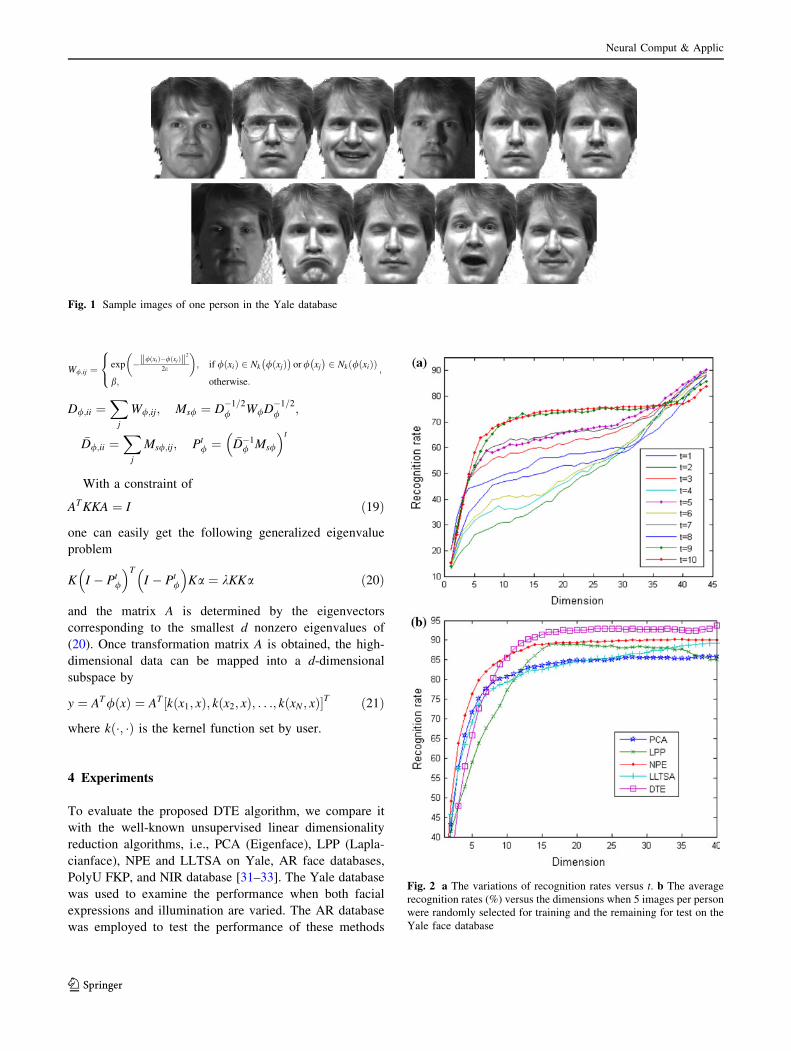
Fig. 1 Sample images of one person in the Yale database

Fig. 2 a The variations of recognition rates versus t. b The average

recognition rates (%) versus the dimensions when 5 images per person

were randomly selected for training and the remaining for test on the

Yale face database


123

under conditions where there was a variation over time, in

facial expressions and in lighting conditions. The FKP

database was used to evaluate the performance when the

images were captured in different time section. The NIR

face database was used to test the performance of different

methods on near-infrared face image recognition with

variations of pose, expression, focus, scale, and time. The

nearest neighbor classifier with Euclidean distance was

used in all the experiments.

4.1 Experiments on Yale database

The Yale face database contains 165 images of 15 indi-

viduals (each person providing 11 different images) under

various facial expressions and lighting conditions. In our

experiments, each image was manually cropped and re-

sized to 100 9 80 pixels. Figure 1 shows sample images of

one person. For computational effectiveness, we down

sample it to 50 9 40 in this experiment.

In order to decide the optimal parameter t, we select 3

images per person for training and the remaining for test in

the experiment. We ran the experiments for 10 times. The

variations of recognition rates versus t are shown in

Fig. 2a. As can be seen from the figure, the optimal

parameter t is t = 5 on this database.

In the experiments, l images (l varies from 3 to 6) are

randomly selected from the image gallery of each individual

to form the training sample set. The remaining 11 – l images

are used for testing. For each l, we independently run the

system 50 times. PCA, LPP, NPE, LLTSA, and DTE are,

respectively, used for feature extraction. In the PCA phase of

LPP, NPE, LLTSA, and DTE, the number of principle

components is set as 40, kept about 96% of the image energy.

The maximal average recognition rate of each method and

the corresponding dimension are given in Table 1. The

average recognition rates (%) versus the dimensions when 5

images per person were randomly selected for training and

the remaining for testing is shown in Fig. 2b.

As it is shown in Table 1 and Fig. 2b, the top recogni-

tion rate of DTE is significantly higher than the compared

methods. Why can DTE significantly outperform the other

algorithms? An important reason may be that DTE not only

characterizes the local geometry structure but also dis-

covers the intrinsic relationships hidden within the data

points at a certain time t steps by introducing dynamic

processes, thus eliminates more negative influence of the

variations of expressions and illuminations.

4.2 Experiments on the AR face database

The AR face database contains over 4,000 color face

images of 126 people (70 men and 56 women), including

frontal views of faces with different facial expressions,

lighting conditions, and occlusions. The pictures of 120

individuals (65 men and 55 women) were taken in two

sessions (separated by 2 weeks), and each section contains

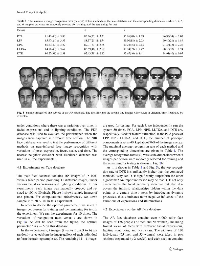
Table 1 The maximal average recognition rates (percent) of five methods on the Yale database and the corresponding dimensions when 3, 4, 5,

and 6 samples per class are randomly selected for training and the remaining for test

#/class 3 4 5 6

PCA 81.47(40) ± 3.83 85.26(37) ± 3.21 85.96(40) ± 1.79 86.93(34) ± 2.03

LPP 85.97(24) ± 3.35 88.57(21) ± 2.74 89.00(18) ± 2.03 90.40(21) ± 1.89

NPE 86.23(39) ± 3.27 89.01(33) ± 2.65 90.24(35) ± 2.13 91.33(32) ± 2.26

LLTSA 84.88(40) ± 3.67 86.59(40) ± 2.82 89.24(39) ± 2.47 90.13(37) ± 1.74

DTE 90.27(38) ± 2.31 92.43(38) ± 2.12 93.67(40) ± 1.41 94.91(40) ± 0.97

Fig. 3 Sample images of one subject of the AR database. The first line and the second line images were taken in different time (separated by

2 weeks)


123

13 color images. 7 images of these 120 individuals are

selected and used in our experiments. The face portion of

each image is manually cropped and then normalized to

50 9 40 pixels. The sample images of one person are

shown in Fig. 3. These images vary as follows: 1. neutral

expression; 2. smiling; 3. angry; 4. screaming; 5. left light

on; 6. right light on; 7. all sides light on; 8. wearing sun

glasses; 9. wearing sun glasses and left light on; and 10.

wearing sun glasses and right light on.

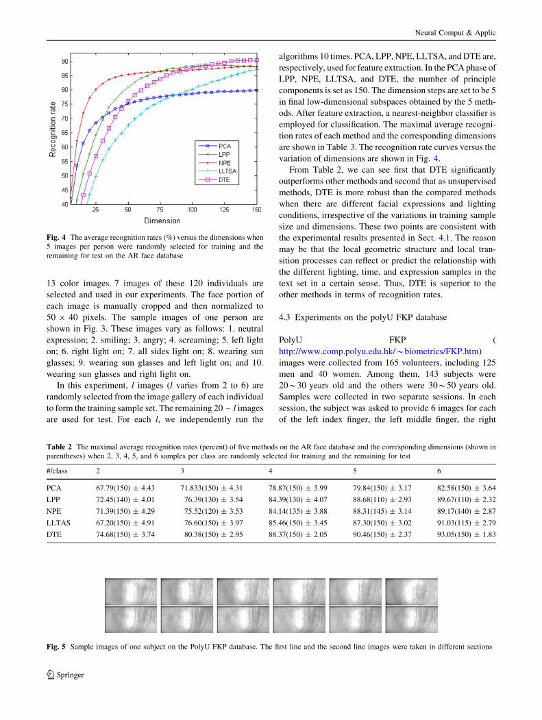
In this experiment, l images (l varies from 2 to 6) are

randomly selected from the image gallery of each individual

to form the training sample set. The remaining 20 – l images

are used for test. For each l, we independently run the

algorithms 10 times. PCA, LPP, NPE, LLTSA, and DTE are,

respectively, used for feature extraction. In the PCA phase of

LPP, NPE, LLTSA, and DTE, the number of principle

components is set as 150. The dimension steps are set to be 5

in final low-dimensional subspaces obtained by the 5 meth-

ods. After feature extraction, a nearest-neighbor classifier is

employed for classification. The maximal average recogni-

tion rates of each method and the corresponding dimensions

are shown in Table 3. The recognition rate curves versus the

variation of dimensions are shown in Fig. 4.

From Table 2, we can see first that DTE significantly

outperforms other methods and second that as unsupervised

methods, DTE is more robust than the compared methods

when there are different facial expressions and lighting

conditions, irrespective of the variations in training sample

size and dimensions. These two points are consistent with

the experimental results presented in Sect. 4.1. The reason

may be that the local geometric structure and local tran-

sition processes can reflect or predict the relationship with

the different lighting, time, and expression samples in the

text set in a certain sense. Thus, DTE is superior to the

other methods in terms of recognition rates.

4.3 Experiments on the polyU FKP database

PolyU FKP (

http://www.comp.polyu.edu.hk/*biometrics/FKP.htm)

images were collected from 165 volunteers, including 125

men and 40 women. Among them, 143 subjects were

20*30 years old and the others were 30*50 years old.

Samples were collected in two separate sessions. In each

session, the subject was asked to provide 6 images for each

of the left index finger, the left middle finger, the right

Fig. 4 The average recognition rates (%) versus the dimensions when

5 images per person were randomly selected for training and the

remaining for test on the AR face database

Table 2 The maximal average recognition rates (percent) of five methods on the AR face database and the corresponding dimensions (shown in

parentheses) when 2, 3, 4, 5, and 6 samples per class are randomly selected for training and the remaining for test

#/class 2 3 4 5 6

PCA 67.79(150) ± 4.43 71.833(150) ± 4.31 78.87(150) ± 3.99 79.84(150) ± 3.17 82.58(150) ± 3.64

LPP 72.45(140) ± 4.01 76.39(130) ± 3.54 84.39(130) ± 4.07 88.68(110) ± 2.93 89.67(110) ± 2.32

NPE 71.39(150) ± 4.29 75.52(120) ± 3.53 84.14(135) ± 3.88 88.31(145) ± 3.14 89.17(140) ± 2.87

LLTAS 67.20(150) ± 4.91 76.60(150) ± 3.97 85.46(150) ± 3.45 87.30(150) ± 3.02 91.03(115) ± 2.79

DTE 74.68(150) ± 3.74 80.38(150) ± 2.95 88.37(150) ± 2.05 90.46(150) ± 2.37 93.05(150) ± 1.83

Fig. 5 Sample images of one subject on the PolyU FKP database. The first line and the second line images were taken in different sections


123

http://www.comp.polyu.edu.hk/~biometrics/FKP.htm

index finger, and the right middle finger. Therefore, 48

images from 4 fingers were collected from each subject. In

total, the database contains 7,920 images from 660 differ-

ent fingers. The average time interval between the first and

the second sessions was about 25 days. The maximum and

minimum intervals were 96 days and 14 days, respectively.

For more details, please see [31, 33]. Some sample images

of one subject on the PolyU FKP database are shown in

Fig. 5.

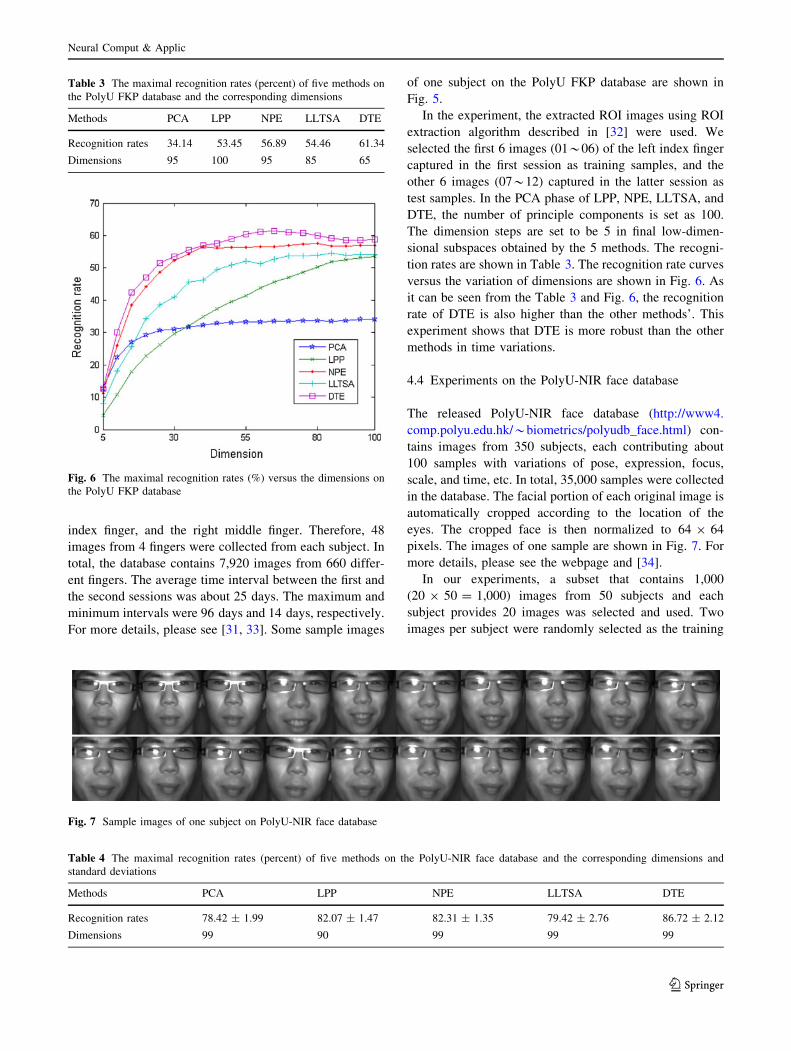
In the experiment, the extracted ROI images using ROI

extraction algorithm described in [32] were used. We

selected the first 6 images (01*06) of the left index finger

captured in the first session as training samples, and the

other 6 images (07*12) captured in the latter session as

test samples. In the PCA phase of LPP, NPE, LLTSA, and

DTE, the number of principle components is set as 100.

The dimension steps are set to be 5 in final low-dimen-

sional subspaces obtained by the 5 methods. The recogni-

tion rates are shown in Table 3. The recognition rate curves

versus the variation of dimensions are shown in Fig. 6. As

it can be seen from the Table 3 and Fig. 6, the recognition

rate of DTE is also higher than the other methods’. This

experiment shows that DTE is more robust than the other

methods in time variations.

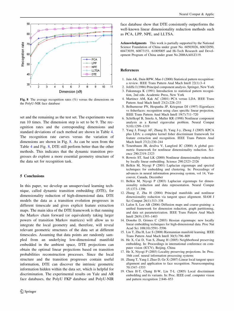
4.4 Experiments on the PolyU-NIR face database

The released PolyU-NIR face database (http://www4.

comp.polyu.edu.hk/*biometrics/polyudb_face.html) con-

tains images from 350 subjects, each contributing about

100 samples with variations of pose, expression, focus,

scale, and time, etc. In total, 35,000 samples were collected

in the database. The facial portion of each original image is

automatically cropped according to the location of the

eyes. The cropped face is then normalized to 64 9 64

pixels. The images of one sample are shown in Fig. 7. For

more details, please see the webpage and [34].

In our experiments, a subset that contains 1,000

(20 9 50 = 1,000) images from 50 subjects and each

subject provides 20 images was selected and used. Two

images per subject were randomly selected as the training

Table 3 The maximal recognition rates (percent) of five methods on

the PolyU FKP database and the corresponding dimensions

Methods PCA LPP NPE LLTSA DTE

Recognition rates 34.14 53.45 56.89 54.46 61.34

Dimensions 95 100 95 85 65

Fig. 6 The maximal recognition rates (%) versus the dimensions on

the PolyU FKP database

Fig. 7 Sample images of one subject on PolyU-NIR face database

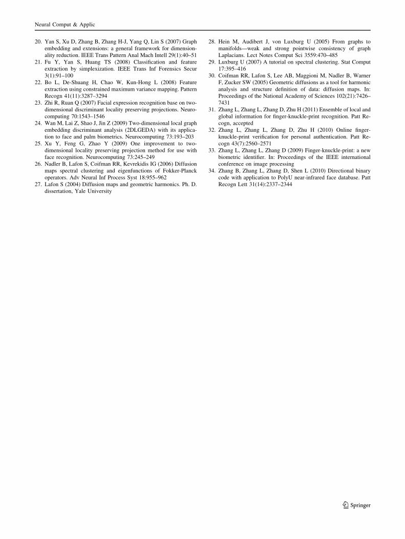
Table 4 The maximal recognition rates (percent) of five methods on the PolyU-NIR face database and the corresponding dimensions and

standard deviations

Methods PCA LPP NPE LLTSA DTE

Recognition rates 78.42 ± 1.99 82.07 ± 1.47 82.31 ± 1.35 79.42 ± 2.76 86.72 ± 2.12

Dimensions 99 90 99 99 99


123

http://www4.comp.polyu.edu.hk/~biometrics/polyudb_face.html

http://www4.comp.polyu.edu.hk/~biometrics/polyudb_face.html

set and the remaining as the test set. The experiments were

run 10 times. The dimension step is set to be 9. The rec-

ognition rates and the corresponding dimensions and

standard deviations of each method are shown in Table 4.

The recognition rate curves versus the variation of

dimensions are shown in Fig. 8. As can be seen from the

Table 4 and Fig. 8, DTE still perform better than the other

methods. This indicates that the dynamic transition pro-

gresses do explore a more essential geometry structure of

the data set for recognition task.

5 Conclusions

In this paper, we develop an unsupervised learning tech-

nique, called dynamic transition embedding (DTE), for

dimensionality reduction of high-dimensional data. DTE

models the data as a transition evolution progresses in

different timescale and gives explicit feature extraction

maps. The main idea of the DTE framework is that running

the Markov chain forward (or equivalently taking larger

powers of transition Markov matrices) will allow us to

integrate the local geometry and, therefore, will reveal

relevant geometric structures of the data set at different

timescales. Assuming that data points are randomly sam-

pled from an underlying low-dimensional manifold

embedded in the ambient space, DTE projections can

obtain the optimal linear projections based on transition

probabilities reconstruction processes. Since the local

structure and the transition progresses contain useful

information, DTE can discover the intrinsic geometric

information hidden within the data set, which is helpful for

discrimination. The experimental results on Yale and AR

face databases, the PolyU FKP database and PolyU-NIR

face database show that DTE consistently outperforms the

well-known linear dimensionality reduction methods such

as PCA, LPP, NPE, and LLTSA.

Acknowledgments This work is partially supported by the National

Science Foundation of China under grant No. 60503026, 60632050,

60473039, 60873151, 61005005 and Hi-Tech Research and Devel-

opment Program of China under grant No.2006AA01Z119.

References

1. Jain AK, Duin RPW, Mao J (2000) Statistical pattern recognition:

a review. IEEE Trans Pattern Anal Mach Intell 22(1):3–4

2. Joliffe I (1986) Principal component analysis. Springer, New York

3. Fukunnaga K (1991) Introduction to statistical pattern recogni-

tion, 2nd edn. Academic Press, New York

4. Martinez AM, Kak AC (2001) PCA versus LDA. IEEE Trans

Pattern Anal Mach Intell 23(2):228–233

5. Belhumeour PN, Hespanha JP, Kriegman DJ (1997) Eigenfaces

vs fisherfaces: recognition using class specific linear projection.

IEEE Trans Pattern Anal Mach Intell 19(7):711–720

6. Scholkopf B, Smola A, Muller KR (1998) Nonlinear component

analysis as a Kernel eigenvalue problem. Neural Comput

5(10):1299–1319

7. Yang J, Frangi AF, Zhang D, Yang J-y, Zhong J (2005) KPCA

plus LDA: a complete kernel fisher discriminant framework for

feature extraction and recognition. IEEE Trans Pattern Anal

Mach Intell 27(2):230–244

8. Tenenbaum JB, desilva V, Langford JC (2000) A global geo-

metric framework for nonlinear dimensionality reduction. Sci-

ence 290:2319–2323

9. Roweis ST, Saul LK (2000) Nonlinear dimensionality reduction

by locally linear embedding. Science 290:2323–2326

10. Belkin M, Niyogi P (2001) Laplacian eigenmaps and spectral

techniques for embedding and clustering. In: Proceedings of

advances in neural information processing system, vol 14, Van-

couver, Canada, December

11. Belkin M, Niyogi P (2003) Laplacian eigenmaps for dimen-

sionality reduction and data representation. Neural Comput

15:1373–1396

12. Zhang Z, Zha H (2004) Principal manifolds and nonlinear

dimensionality reduction via tangent space alignment. SIAM J

Sci Comput 26(1):313–338

13. Lafon S, Lee AB (2006) Diffusion maps and coarse-graining: a

unified framework for dimension reduction, graph partitioning,

and data set parameterization. IEEE Trans Pattern Anal Mach

Intell 28(9):1393–1403

14. Donoho D, Grimes C (2003) Hessian eigenmaps: new locally

linear embedding techniques for high-dimensional data. Proc Nat

Acad Sci 100(10):5591–5596

15. Lin T, Zha H, Lee S (2008) Riemannian manifold learning. IEEE

Trans Pattern Anal Mach Intell 30(5):796–809

16. He X, Cai D, Yan S, Zhang H (2005) Neighborhood preserving

embedding. In: Proceedings in international conference on com-

puter vision (ICCV), Beijing, China

17. He X, Niyogi P (2003) Locality preserving projections. In: Proc.

16th conf. neural information processing systems

18. Zhang T, Yang J, Zhao D, Ge X (2007) Linear local tangent space

alignment and application to face recognition. Neurocomputing

70:1547–1553

19. Chen H-T, Chang H-W, Liu T-L (2005) Local discriminant

embedding and its variants. In: Proc. IEEE conf. computer vision

and pattern recognition 2:846–853

Fig. 8 The average recognition rates (%) versus the dimensions on

the PolyU-NIR face database


123

20. Yan S, Xu D, Zhang B, Zhang H-J, Yang Q, Lin S (2007) Graph

embedding and extensions: a general framework for dimension-

ality reduction. IEEE Trans Pattern Anal Mach Intell 29(1):40–51

21. Fu Y, Yan S, Huang TS (2008) Classification and feature

extraction by simplexization. IEEE Trans Inf Forensics Secur

3(1):91–100

22. Bo L, De-Shuang H, Chao W, Kun-Hong L (2008) Feature

extraction using constrained maximum variance mapping. Pattern

Recogn 41(11):3287–3294

23. Zhi R, Ruan Q (2007) Facial expression recognition base on two-

dimensional discriminant locality preserving projections. Neuro-

computing 70:1543–1546

24. Wan M, Lai Z, Shao J, Jin Z (2009) Two-dimensional local graph

embedding discriminant analysis (2DLGEDA) with its applica-

tion to face and palm biometrics. Neurocomputing 73:193–203

25. Xu Y, Feng G, Zhao Y (2009) One improvement to two-

dimensional locality preserving projection method for use with

face recognition. Neurocomputing 73:245–249

26. Nadler B, Lafon S, Coifman RR, Kevrekidis IG (2006) Diffusion

maps spectral clustering and eigenfunctions of Fokker-Planck

operators. Adv Neural Inf Process Syst 18:955–962

27. Lafon S (2004) Diffusion maps and geometric harmonics. Ph. D.

dissertation, Yale University

28. Hein M, Audibert J, von Luxburg U (2005) From graphs to

manifolds—weak and strong pointwise consistency of graph

Laplacians. Lect Notes Comput Sci 3559:470–485

29. Luxburg U (2007) A tutorial on spectral clustering. Stat Comput

17:395–416

30. Coifman RR, Lafon S, Lee AB, Maggioni M, Nadler B, Warner

F, Zucker SW (2005) Geometric diffusions as a tool for harmonic

analysis and structure definition of data: diffusion maps. In:

Proceedings of the National Academy of Sciences 102(21):7426–

7431

31. Zhang L, Zhang L, Zhang D, Zhu H (2011) Ensemble of local and

global information for finger-knuckle-print recognition. Patt Re-

cogn, accepted

32. Zhang L, Zhang L, Zhang D, Zhu H (2010) Online finger-

knuckle-print verification for personal authentication. Patt Re-

cogn 43(7):2560–2571

33. Zhang L, Zhang L, Zhang D (2009) Finger-knuckle-print: a new

biometric identifier. In: Proceedings of the IEEE international

conference on image processing

34. Zhang B, Zhang L, Zhang D, Shen L (2010) Directional binary

code with application to PolyU near-infrared face database. Patt

Recogn Lett 31(14):2337–2344


123

Dynamic transition embedding for image feature extraction and recognition

Documents

Transcript of Dynamic transition embedding for image feature extraction and recognition