1

3

5

7

9

11

13

15

17

19

21

23

25

27

29

31

33

35

37

39

41

43

45

47

49

51

53

55

ARTICLE IN PRESS

3B2v8:06a=w ðDec 5 2003Þ:51cXML:ver:5:0:1 CAG : 1405 Prod:Type:FTP

pp:1212ðcol:fig::F1;2;6213ÞED:ShanthiV:B:

PAGN:Vishwanath SCAN:Padma

0097-8493/$ - se

doi:10.1016/j.ca

�CorrespondE-mail add

lbarthe@irit.fr

Computers & Graphics ] (]]]]) ]]]–]]]

www.elsevier.com/locate/cag

Dynamic surfel set refinement for high-quality rendering

Gael Guennebaud�, Loıc Barthe, Mathias Paulin

IRIT, CNRS, Universite Paul Sabatier, 118 route de Narbonne, 31062 Toulouse, Cedex 4, France

TED PROOFAbstract

Splatting-based rendering techniques are currently the best choice for efficient high-quality rendering of point-based

geometries. However, such techniques are not suitable for large magnification, especially when the object is under-

sampled. This paper improves the rendering quality of pure splatting techniques using a fast dynamic up-sampling

algorithm for point-based geometry. Our algorithm is inspired by interpolatory subdivision surfaces where the

geometry is refined iteratively. At each step the refined geometry is that from the previous step enriched by a new set of

points. The point insertion procedure uses three operators: a local neighborhood selection operator, a refinement

operator (adding new points) and a smoothing operator. Even though our insertion procedure makes the analysis of the

limit surface complicated and it does not guarantee its G1 continuity, it remains very efficient for high-quality real-time

point rendering. Indeed, while providing an increased rendering quality, especially for large magnification, our

algorithm needs no other preprocessing nor any additional information beyond that used by any splatting technique.

This extended version (Real-time point cloud refinement, in: Proceedings of Eurographics Symposium on Point-Based

Graphic, 2004, pp. 41.) contains details on creases handling and more comparison to other smoothing operators.

r 2004 Published by Elsevier Ltd.

Keywords: I.3.3; I.3.5; Viewing algorithms; Curve; Surface; Solid; Object representations

C 57

59

61

63

65

67

69

UNCORRE1. Introduction

Owing to the absence of topological information,

point clouds give us a simple and powerful surface

representation for complex geometries where the accu-

racy mainly depends on the number of points. However,

real-time visualization of such data sets requires addi-

tional information such as normal vector, texture color,

and an estimation of the local sampling density. From

these additional attributes, a continuous image of the

point cloud can be reconstructed using an image-based

filtering technique, by adjusting the sampling density on

the fly or by using the so-called surface splatting

71

73

e front matter r 2004 Published by Elsevier Ltd.

g.2004.08.011

ing author.

resses: guenneba@irit.fr (G. Guennebaud),

(L. Barthe), paulin@irit.fr (M. Paulin).

technique [1]. In the latter case, each point is represented

by an oriented disk (a surfel) in object space [2].

Rendering is then equivalent to a resampling process

where surfels are blended with a Gaussian distribution in

the image space. In this paper, we call such a point cloud

a surfel set. Currently, for high-quality and efficient

point-based rendering, a splatting approach is doubtless

the best choice since such approaches are supported by

modern GPUs [3,4].

Whereas a surfel set describes a continuous texture

function [1], from the geometric point of view it is a

simple set of oriented overlapping disks. Hence, in the

case of an under-sampled surface, visual artifacts appear

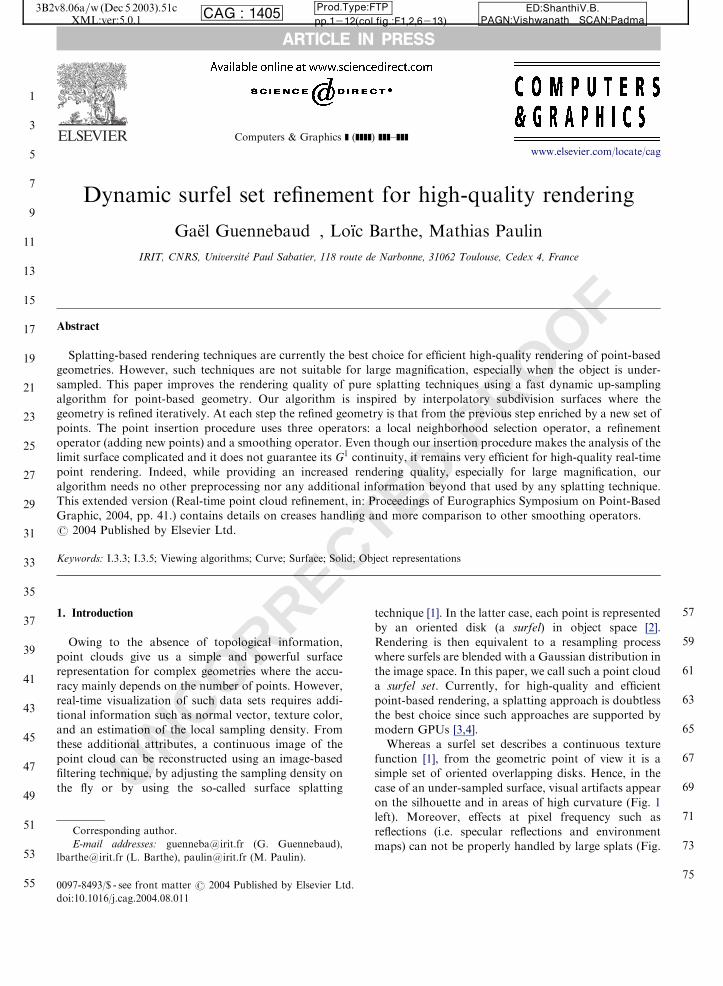
on the silhouette and in areas of high curvature (Fig. 1

left). Moreover, effects at pixel frequency such as

reflections (i.e. specular reflections and environment

maps) can not be properly handled by large splats (Fig.

75

1

3

5

7

9

11

13

15

17

19

21

23

25

27

29

31

33

35

37

39

41

43

45

47

49

51

53

55

57

59

61

63

65

67

69

71

73

75

77

79

81

83

85

87

89

91

93

95

97

99

101

103

105

107

109

111

ARTICLE IN PRESSCAG : 1405

Fig. 1. Left: rendering of an undersampled bunny with a pure

high-quality splatting technique. Artifacts on silhouette and

specular reflexions are clearly visible. Right: same model with

our dynamic up-sampling algorithm enabled.

G. Guennebaud et al. / Computers & Graphics ] (]]]]) ]]]–]]]2

UNCORREC9). Thus, for high-quality rendering, the use of a pure

splatting-based approach is limited to relative small

magnification.

Although a point set intrinsically describes a smooth

surface, the geometry itself is discontinuous. This can be

compared to polygonal meshes where the geometry is

only C0 continuous even though we may intend the

mesh to describe a smooth (G1) surface. In order to

overcome the continuity problem of polygonal meshes,

several methods have been developed. Among these,

subdivision surfaces perform the refinement of a coarse

mesh into a finer one and several iterations generate a

sequence of incrementally refined meshes which con-

verges to a smooth surface [5–8]. More specifically,

interpolatory subdivision schemes [9–11] are well suited

when we desire smooth interpolation of the mesh

vertices. Following the same idea, a point set could be

refined in order to maintain local point density and

hence improve rendering quality. Unfortunately, owing

to the lack of topological information, subdivision

operators for meshes cannot be directly applied to point

sets.

On the other hand, several consolidationmethods have

been proposed. By consolidation we mean the process of

extrapolating a continuous surface from the point set.

Most consolidation methods are based on an implicit

representation. For example, in [12], a triangular mesh is

built from a signed distance function defined on a

volumetric grid. Others are based on radial basis

TED PROOF

functions (RBF) that reconstruct a Cn implicit surface

from a scattered point set [13]. However, owing to the

global support of RBFs, such approaches need an

expensive preprocessing step since the coefficients of the

RBFs are computed by solving a large linear system.

This problem is partially overcome by local approaches

[14,15], but they remain too expensive for real-time

applications.

In [16], Levin introduces a smooth point-based

representation called moving least-squares (MLS) sur-

face. The surface is defined implicitly by a local

projection operator. A related definition of a smooth

surface from points is the implicit version of Adamson

and Alexa [17] that allows relatively fast ray intersection

(5k intersections per second), surface boundaries repre-

sentation [18] and accurate normal computation [19]. In

[20] Amenta and Kil describe the MLS surface as an

extremal surface. They also define a similar surface

determined by a set of surfels.

Based on the MLS surface representation, several

methods for down-sampling [21,22] and up-sampling

[21,23] point sets have been proposed. However, these

up-sampling methods are not suitable for real-time

applications since the computation of the local projec-

tion operator is a non-linear optimization problem.

Moreover, methods used for the generation of a locally

uniform sampling are expensive to evaluate since they

are based on either a local Voronoı diagram or a particle

simulation [24]. In [21] Alexa et al. present an interactive

rendering technique based also on the MLS surface

representation. In a preprocessing step, a bivariate

polynomial is computed for each point of the reference

point set. During rendering, additional points can be

dynamically sampled from these polynomials. In addi-

tion to the need for preprocessing, this up-sampling

approach presents other drawbacks: it does not support

discontinuities or texture colors, it requires much

memory for storing the polynomials, and it generates

oversampling owing to the overlapping of polynomials

patches.

In [25], Stamminger and Drettakis render complex

procedural geometry with a dynamicffiffiffi5p

sampling

algorithm. While their sampling scheme is fast to

evaluate, its extension to the smooth up-sampling of

general point-based geometries is difficult.

In order to increase the rendering quality of surfel

sets, we present a new up-sampling method inspired by

subdivision surfaces. The main features of our algorithm

are:

�

Speed: Real-time processing is our major constraint.

�

Simplicity: Easy to implement and adapted to further

hardware optimizations.

�

Smoothness: The visualized surface looks smooth.

�

Locally uniform sampling: Avoiding oversampling is a

fundamental issue, especially for hardware splatting

1

3

5

7

9

11

13

15

17

19

21

23

25

27

29

31

33

35

37

39

41

43

45

47

49

51

53

55

57

ARTICLE IN PRESSCAG : 1405

G. Guennebaud et al. / Computers & Graphics ] (]]]]) ]]]–]]] 3

approaches that are limited by the precision of the

color buffer.

59

� Globally adaptive sampling: Only areas that need

accurate sampling are refined.

61

� Suitable for discontinuities: Our method handles

boundaries and sharp creases.

63

�

PROOF

65

67

69

71

73

75

77

79

81

83

85

87

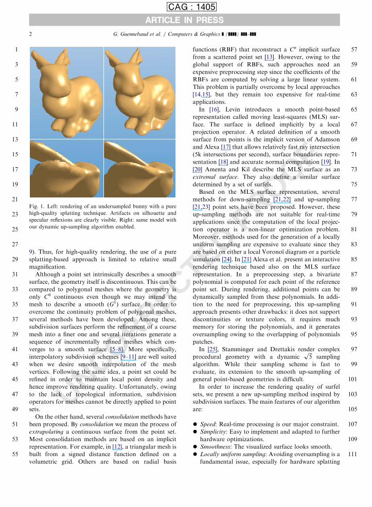
Fig. 2. Illustration of the refinement procedure. On the top left,

the initial points (from the bunny model) are visualized with

large white surfels. The smaller points have been introduced by

a single refinement step. The red point comes from the

interpolation of five points. From left to right and top to

bottom, one refinement step is performed on the input points

(coming from the previous refinement step and visualized with

large surfels).

No preprocessing: Our system takes as input an

unstructured point set with per point normal, texture

color and radius. This set of attributes is the

minimum information needed for all point based

rendering techniques. Because our algorithm does not

need any preprocessing, it is well-suited for handling

deformable models.

Since real-time processing is our major constraint, we

decided to develop an interpolation method which is as

fast as possible. Even though we cannot guarantee its G1

continuity, the approach presented here increases the

rendering quality of a pure splatting technique.

The paper is organized as follow: after a brief

overview of our refinement algorithm in Section 2, we

describe the local point of view in Section 3 and the

global point of view in Section 4. Then we show how our

refinement procedure can be efficiently used on top of a

rendering pipeline (Section 5). From the earlier version

[26], in addition to give more details on the dynamic

refinement procedure, we explain in detail how sharp

features are handled (boundaries and creases) in the

Section 3.2.2. We also add performance and quality

comparisons of our method to the butterfly scheme and

MLS projection operator in the Section 6.1.

89

91

93

95

97

99

101

103

105

107

109

111

UNCORREC2. Overview

Our algorithm takes, as input, a regular point set P0 ¼

fpig defining a smooth surface. We assume that we also

know, for each point pi 2 P; its normal ~ni; its texture

color and the local density described by a scalar radius

ri: The radius, ri; of each surfel has to be large enough to

provide a splatting rendering without holes, and it must

be less than or equal to the maximum distance between

the ith surfel and its neighbors. The initial point set, P0;is up-sampled by inserting additional points yielding the

new set P1 with P0 � P1: In a similar fashion to

subdivision surfaces, the up-sampled point set describes

a new surface that is used for the next refinement step.

At each refinement step, the number of points approxi-

mately quadruples, increasing the resolution by a factor

of two (Fig. 2). Hence, the radius of surfels are divided

by two at each step. By repeating the refinement step we

construct a sequence P0;P1; . . . of point sets with Pl �

Plþ1:Our up-sampling algorithm can be described by a

selection operator C and an interpolation operator F:The selection operator (see Section 3.1 and Fig. 4) takes

TEDa point p 2 Pl and defines the set CðpÞ of point subsetsCiðpÞ around p from which a single new point will be

inserted:

C : Pl�!PðPðPlÞÞ;

C : p7�!fC0ðpÞ; . . . ;CmðpÞg(1)

with PðEÞ the power set of the set E : PðEÞ ¼ fe j e �Eg: The operator F (Section 3.2) inserts a single new

point by interpolation of the points of CiðpÞ: Hence for

each CiðpÞ; a new point is added to Plþ1:

F : PðPlÞ�!R3 (2)

and the up-sampled point set Plþ1 of Pl is defined as

follows:

Plþ1 ¼ Pl [ fFðCiðpÞÞ jCiðpÞ 2 CðpÞ; 8p 2 Plg: (3)

For convenience, attributes of points (normals, colors,

etc.) do not appear in these definitions. As mentioned in

Section 4, the global subdivision process must be slightly

modified to avoid redundancy. However, before describ-

ing the global subdivision algorithm (Section 4), we first

present in detail the refinement procedure around a

single point p 2 Pl ; by describing the local operators Cand F:

F

1

3

5

7

9

11

13

15

17

19

21

23

25

27

29

31

33

35

37

39

41

43

45

47

49

51

53

55

57

59

61

63

65

67

69

71

73

75

ARTICLE IN PRESSCAG : 1405

G. Guennebaud et al. / Computers & Graphics ] (]]]]) ]]]–]]]4

3. Local up-sampling

3.1. The selection operator, C

Our up-sampling scheme is based on the idea of

adding a new point for each pair of neighbor samples.

However, whatever the accuracy of the neighbor

relation, this basic idea is insufficient because a subset

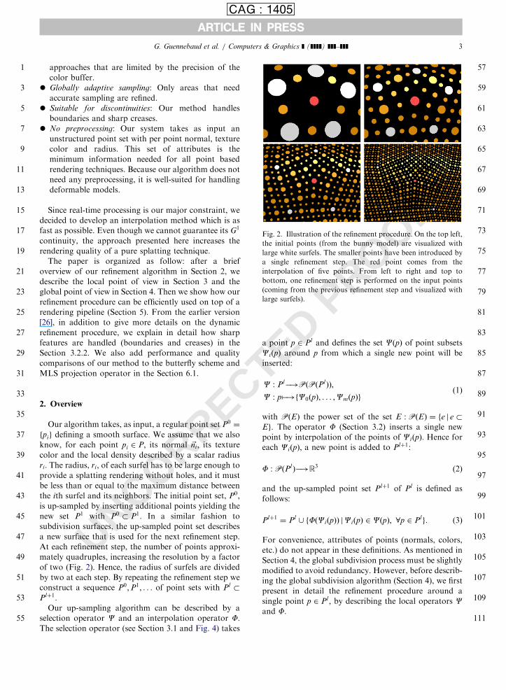
of kX4 points that are all in the neighborhood of one

another generates 12kðk � 3Þ points near their center

(Figs. 3a, 4b). In such cases, the obvious choice is to

insert only a single new point.

From a given point p 2 P and its neighborhood Np �

P (Section 3.1.1), the selection operator C must define a

set of subsets of points in Np for which a single new

point must be inserted. This is done by building a local

set of polygons, called a polygon fan, from the implicit

triangle fan defined by the neighborhoods (Section

3.1.2). This construction is similar to the fan cloud

representation of Linsen and Prautzsch [27].

UNCORRECFig. 3. (a) Four surfels are all in the neighborhood of one

another. Interpolating points two by two leads to over-

sampling and incoherency. (b) The query ball intersects two

disjoint components of the surface.

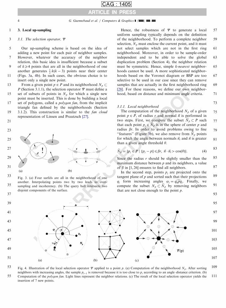
Fig. 4. Illustration of the local selection operator C applied to a po

neighbors with increasing angles, the sample pi�1 is removed because

Computation of the polygon fan. Light lines represent the neighbor r

insertion of 7 new points.

Hence, the robustness of C to generate a local

uniform sampling typically depends on the definition

of the neighborhood. To perform a complete neighbor

selection, Np must enclose the current point, and it must

not select samples which are not in the first ring

neighborhood. Moreover, in order to be sample-order

independent and to be able to solve the global

duplication problem (Section 4), the neighbor relation

must be symmetric. Hence, simple k-nearest neighbor-

hoods cannot be used. A more sophisticated neighbor-

hoods based on the Voronoi diagram or BSP are too

selective to be used in our case since they can remove

samples that are actually in the first neighborhood ring

[28]. For these reasons, we define our own neighbor-

hood, based on distance and minimum angle criteria.

77

79

81

83

85

87

89

91

TED PROO3.1.1. Local neighborhood

The computation of the neighborhood Np of a given

point p 2 P; of radius r and normal ~n is performed in

two steps. First, we compute the subset eNp � P such

that each point pi 2 eNp is in the sphere of center p and

radius br: In order to avoid problems owing to fine

‘‘features’’ (Figure 3b), we also remove from eNp points

for which the angle between normals ~ni and ~n is greater

than a given angle threshold y:

eNp ¼ fpi 2 P j kpi � pkpbr; ~n �~ni4 cosðyÞg: (4)

Since the radius r should be slightly smaller than the

maximum distance between p and its neighbors, a value

of b in ½1; 26� ensures to find all neighbors.

In the second step, points pi are projected onto the

tangent plane of p and sorted such that their projections

qi form increasing angles ji ¼ dq0pqi: Finally, we

compute the subset Np � eNp by removing neighbors

that are not close enough to the point p.

93

95

97

99

101

103

105

107

109

111

int p. (a) Computation of the neighborhood Np: After sorting

it is too close to pi according to an angle–distance criterion. (b)

elations. (c) The result of the local selection operator yields the

1

3

5

7

9

11

13

15

17

19

21

23

25

27

29

31

33

35

37

39

41

43

45

47

49

51

53

55

57

59

61

63

65

67

69

71

73

75

77

79

81

83

85

87

89

91

93

95

97

99

101

103

105

107

109

111

ARTICLE IN PRESSCAG : 1405

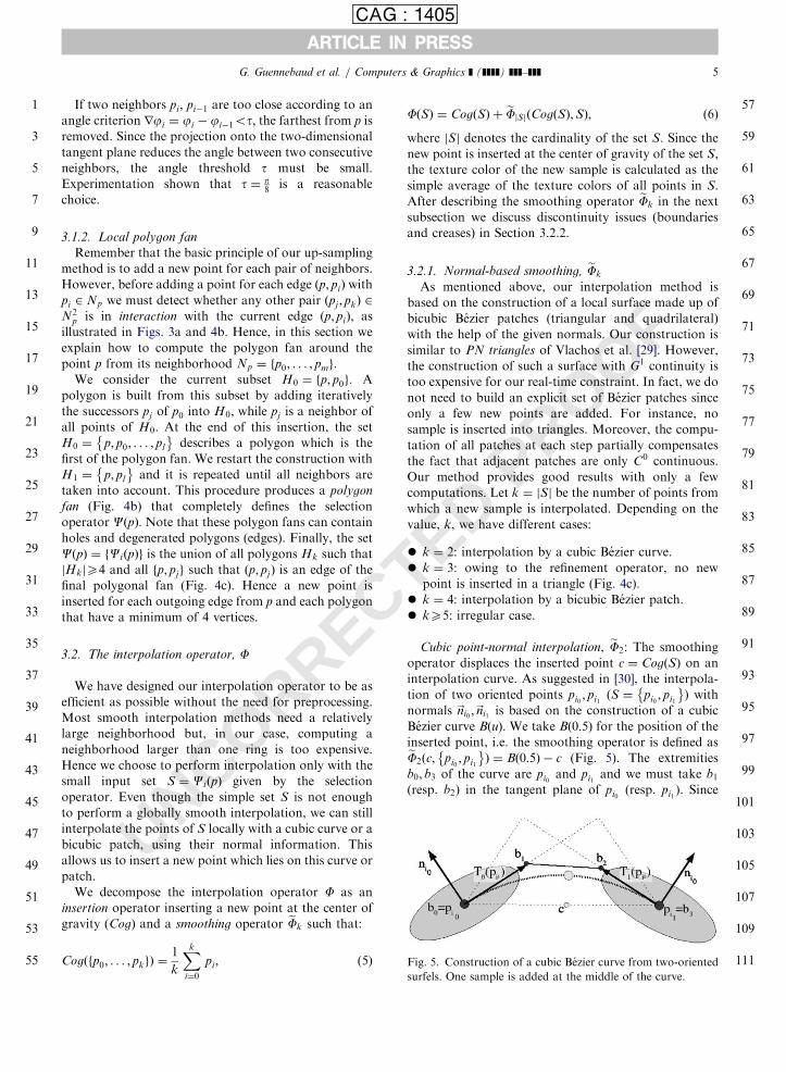
Fig. 5. Construction of a cubic Bezier curve from two-oriented

surfels. One sample is added at the middle of the curve.

G. Guennebaud et al. / Computers & Graphics ] (]]]]) ]]]–]]] 5

UNCORREC

If two neighbors pi; pi�1 are too close according to an

angle criterion rji ¼ ji � ji�1ot; the farthest from p is

removed. Since the projection onto the two-dimensional

tangent plane reduces the angle between two consecutive

neighbors, the angle threshold t must be small.

Experimentation shown that t ¼ p8

is a reasonable

choice.

3.1.2. Local polygon fan

Remember that the basic principle of our up-sampling

method is to add a new point for each pair of neighbors.

However, before adding a point for each edge ðp; piÞ withpi 2 Np we must detect whether any other pair ðpj ; pkÞ 2N2

p is in interaction with the current edge ðp; piÞ; as

illustrated in Figs. 3a and 4b. Hence, in this section we

explain how to compute the polygon fan around the

point p from its neighborhood Np ¼ fp0; . . . ; pmg:We consider the current subset H0 ¼ fp; p0g: A

polygon is built from this subset by adding iteratively

the successors pj of p0 into H0; while pj is a neighbor of

all points of H0: At the end of this insertion, the set

H0 ¼ p; p0; . . . ; pl� �

describes a polygon which is the

first of the polygon fan. We restart the construction with

H1 ¼ p; pl� �

and it is repeated until all neighbors are

taken into account. This procedure produces a polygon

fan (Fig. 4b) that completely defines the selection

operator CðpÞ: Note that these polygon fans can contain

holes and degenerated polygons (edges). Finally, the set

CðpÞ ¼ fCiðpÞg is the union of all polygons Hk such that

jHkjX4 and all fp; pjg such that ðp; pjÞ is an edge of the

final polygonal fan (Fig. 4c). Hence a new point is

inserted for each outgoing edge from p and each polygon

that have a minimum of 4 vertices.

3.2. The interpolation operator, F

We have designed our interpolation operator to be as

efficient as possible without the need for preprocessing.

Most smooth interpolation methods need a relatively

large neighborhood but, in our case, computing a

neighborhood larger than one ring is too expensive.

Hence we choose to perform interpolation only with the

small input set S ¼ CiðpÞ given by the selection

operator. Even though the simple set S is not enough

to perform a globally smooth interpolation, we can still

interpolate the points of S locally with a cubic curve or a

bicubic patch, using their normal information. This

allows us to insert a new point which lies on this curve or

patch.

We decompose the interpolation operator F as an

insertion operator inserting a new point at the center of

gravity (Cog) and a smoothing operator eFk such that:

Cogðfp0; . . . ; pkgÞ ¼1

k

Xki¼0

pi; (5)

PROOF

FðSÞ ¼ CogðSÞ þ eFjSjðCogðSÞ;SÞ; (6)

where jSj denotes the cardinality of the set S: Since the

new point is inserted at the center of gravity of the set S;the texture color of the new sample is calculated as the

simple average of the texture colors of all points in S.

After describing the smoothing operator eFk in the next

subsection we discuss discontinuity issues (boundaries

and creases) in Section 3.2.2.

3.2.1. Normal-based smoothing, eFk

As mentioned above, our interpolation method is

based on the construction of a local surface made up of

bicubic Bezier patches (triangular and quadrilateral)

with the help of the given normals. Our construction is

similar to PN triangles of Vlachos et al. [29]. However,

the construction of such a surface with G1 continuity is

too expensive for our real-time constraint. In fact, we do

not need to build an explicit set of Bezier patches since

only a few new points are added. For instance, no

sample is inserted into triangles. Moreover, the compu-

tation of all patches at each step partially compensates

the fact that adjacent patches are only C0 continuous.

Our method provides good results with only a few

computations. Let k ¼ jSj be the number of points from

which a new sample is interpolated. Depending on the

value, k, we have different cases:

�

D

k ¼ 2: interpolation by a cubic Bezier curve.

�

Ek ¼ 3: owing to the refinement operator, no new

point is inserted in a triangle (Fig. 4c).

T� k ¼ 4: interpolation by a bicubic Bezier patch.

�

kX5: irregular case.

Cubic point-normal interpolation, eF2: The smoothing

operator displaces the inserted point c ¼ CogðSÞ on an

interpolation curve. As suggested in [30], the interpola-

tion of two oriented points pi0 ; pi1 (S ¼ pi0 ; pi1� �

) with

normals ~ni0 ;~ni1 is based on the construction of a cubic

Bezier curve BðuÞ: We take Bð0:5Þ for the position of the

inserted point, i.e. the smoothing operator is defined aseF2ðc; pi0 ; pi1� �

Þ ¼ Bð0:5Þ � c (Fig. 5). The extremities

b0; b3 of the curve are pi0 and pi1 and we must take b1(resp. b2) in the tangent plane of pi0 (resp. pi1 ). Since

1

3

5

7

9

11

13

15

17

19

21

23

25

27

29

31

33

35

37

39

41

43

45

47

49

51

53

55

57

59

61

63

65

67

69

71

73

75

77

79

81

83

85

87

89

91

93

95

97

99

101

103

105

107

109

111

ARTICLE IN PRESSCAG : 1405

G. Guennebaud et al. / Computers & Graphics ] (]]]]) ]]]–]]]6

UNCORREC

there is an infinite number of solutions, we take one

which is both convenient to compute and of reasonable

shape. Let b01 be the projection of the point pi1 into the

tangent plane of pi0 : We take b1 such that b0b1��!¼ n b0b

01

��!:

The n scalar defines the velocity of the curve and it must

be close to 13for visually good results [29]. Let TiðqÞ be

the tangent vector from pi toward q,

TiðqÞ:¼nkpi � qkðq� ððpi � qÞ �~niÞ~niÞ

kðq� ððpi � qÞ �~niÞ~niÞk: (7)

Hence we have,

eF2ðc; fpi0 ; pi1 gÞ ¼3

8ðTi0 ðpi1 Þ þ Ti1 ðpi0 ÞÞ: (8)

In order to compute the normal ~n of the new point p ¼eF2 c; pi0 ; pi1� �� �

we first compute the curve tangent_Bð0:5Þ and we take a perpendicular vector. Again, there

is an infinite number of solutions, and a reasonable

choice is to take the normal which is the closest to the

two input normals, i.e. the vector which is in the plane of

normal ~nplane:

~nplane ¼ ð~ni0 þ~ni1 Þ ^ ðpi1 � pi0 Þ;

~n ¼ ~nplane ^ _Bð0:5Þ: ð9Þ

Another possibility is to perform a quadratic interpola-

tion of the normals as in [31]. This solution is

computationally equivalent but it generates more

oscillations.

Bicubic point-normal interpolation, eF4: When a point

has been inserted from four surfels, its displacement can

be computed from a bicubic Bezier patch Bðu; vÞ: We

take eF4ðc; pi0 ; . . . ; pi3� �

Þ ¼ Bð0:5; 0:5Þ � c as the smooth-

ing displacement vector. The position of the 4 corner

Bezier points are pi0 ; . . . ; pi3 : The 8 control points at the

boundary of the patch are computed as in the previous

case. For the 4 interior Bezier points the simpler solution

is to take the zero twists method [30]. We have, for the

corner point pi0 :

b00 ¼ pi0 ;

b01 ¼ b00 þ Ti0 ðpi1 Þ;

b10 ¼ b00 þ Ti0 ðpi3 Þ;

b11 ¼ b00 þ Ti0 ðpi1 Þ þ Ti0 ðpi3 Þ:

The normal is given by the cross product of the two

tangents of the Bezier patch.

Generalized point-normal interpolation, eFk; kX5:

While it is possible to construct patches with an

arbitrary number of edges [30], we propose here a

simpler method. Indeed, such irregular cases appear only

during the first refinement step and with a small

frequency. By extension to the two regular previous

cases, we compute the displacement of the inserted point

c from the interpolation of k surfels, with kX5; as

follows:

OOF

eFkðc; fpi0 ; . . . ; pik�1 gÞ ¼3

4k

Xk�1j¼0

2Tij ðcÞ: (10)

The computation of the normal cannot be generalized in

the same manner. A reasonable solution is to take the

average of the k normals resulting of the k cross

products: ðpij�1 � pÞ ^ ðpij � pÞ:While we give a generalized case for polygons with

kX5 edges, in practice we never met cases with k45:This is principally due to both the minimum angle

criterion in our neighborhood definition that forces the

selection of mostly regular polygons and the regularity

of the input point set. Indeed, we notice that the

robustness of our method directly depends of the

sampling regularity. It is also possible to avoid such

cases by splitting polygons into triangles and quads, but

by doing so, several points will be inserted in the

polygon, yielding to a less uniform sampling. Moreover,

this can introduce more oscillations since all vertices do

not participate equally in the interpolation. The refine-

ment of a such case is illustrated Fig. 2.

TED PR

3.2.2. Boundaries and creases

Discontinuities such as boundaries and creases can be

easily handled by our approach. Indeed, boundaries do

not need special treatment if we assume that the

boundary line passes through the center of the boundary

surfels. Creases are handled using an explicit crease line

representation as in [23]. In this case a surfel stores two

different normals and two different colors. From a surfel

with two normals, we derive two clipped surfels and the

clipping line direction is the cross product of the two

normals. This line direction is used both for the

rendering, i.e. in order to clip surfels, and for the

interpolation. Indeed, the construction of Bezier curves

and patches requires the computation of the tangent

vector from a surfel p0 toward another one p1: Threecases are to be distinguished:

1.

p0 is a simple surfel: no change. The projection of p1onto the tangent plane of p0 gives us the direction of

the tangent vector (Eq. 7).

2.

p0 has two normals n01 ; n02 and p1 satisfies the

condition:

cl0

kcl0k�

p1 � p0kp1 � p0k

��������4 cosðTcÞ; (11)

where cl0 is the clipping line direction of the two

tangent planes of p0 : cl0 ¼ n01 ^ n02 : In this case, the

direction of the tangent vector from p0 toward p1 is

cl0 (or �cl0 if cl0 � ðp1 � p0Þo0). This condition

defines a cone of aperture Tc that determines if p1is on the crease or not. The choice for the value of Tc

depends on the type of p1: Indeed, if p1 has also two

different normals, the tolerance angle must be

1

3

5

7

9

11

13

15

17

19

21

23

25

27

29

31

33

35

37

39

41

43

45

47

49

51

53

55

57

59

61

ARTICLE IN PRESSCAG : 1405

G. Guennebaud et al. / Computers & Graphics ] (]]]]) ]]]–]]] 7

relatively large (Fig. 10 first row), 3p8is a reasonable

value. On the other hand, if p1 is a simple surfel we

must blend the sharp features with the smooth

surface (Figure 10 second row). This implies a small

angle (after experiments we suggest p6).

3.

O

63

65

67

69

71

73

75

77

79

81

83

85

87

89

91

93

95

97

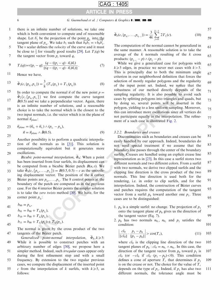
Fig. 6. Left: the point p is refined and 4 new points are inserted

while the red edge overlaps two other polygons. Right: the

point p is removed and the points p0 is refined. A wrong new

point is inserted between p0; p2: Then, p1 is refined and another

wrong point is inserted between p1; p3: This problem is solved

during the refinement of p by inserting p2 into the black list of

p0 and p3 into the black list of p1:

RREC

the last case is when p0 has two normals and p1 does

not satisfy condition (11). We take the tangent vector

as in case 1 by projecting p1 onto the two tangent

planes of p0 and we keep the projected point which is

the closest to p1:

Six combinations are possible for the interpolation

between two surfels p0 and p1: Three of them are

explicitly illustrated Fig. 10. The new inserted surfel will

have two different normals if and only if one of the

extremities p0 and p1 is in the case 2. The two normals of

the new surfel are computed with Eq. (9). For the

quadrilateral case, before inserting a new point in the

middle of a bicubic Bezier patch we must check if a

crease line does not pass through the quad, i.e. if two

opposite surfels of the quad are not both in case 2. In

this case the two other corners are discarded and a new

surfel with two normals is inserted onto the crease line

(case 2-2). Corners are treated in a similar manner,

simply they require three different normals. Each of

these normals defines a tangent plane in p0: The normal

defining the tangent plane which is the farthest to p1 is

discarded. Then, two normals remain and the surfel is

treated as in cases 2 and 3.

However, if creases are not explicitly represented in

the reference point cloud geometry, they can be detected

during the first subdivision step. If the angle between the

tangent planes of two neighbor points p and p0 is greater

than a given crease angle, a new surfel with its two

normals is inserted at the intersection between the crease

line (intersection of the two tangent planes) and the

plane defined by the two points p and p0 and the vector~nplane (computed as in Eq. (9) using p, p0 and their

normals). Full details on the rendering of sharp features

can be found in [23,32]. It is also possible to use, in a

preprocessing step, a more robust and automatic feature

detection algorithm [33].

O99

101

103

105

107

109

UNC4. Global up-sampling algorithm

In the previous section we have shown how a given

point neighborhood is refined into several points with

local uniformity. However, the direct subdivision of a

point set Pl to Plþ1 with the basic formulation (Eq. (3))

generates multiple duplicated samples: points generated

from k samples appear k times in Plþ1: In order to avoid

these duplications, we first remove from Pl the current

processed point. Hence, Plþ1 is computed as follow:

for

each p 2 Pl do

Plþ1 Plþ1 [ fFðSiÞ jSi 2 CðpÞg

FPl Pl � fpg

done

111

TED PRO

Another problem is the overlapping of neighbor

relations (Fig. 6) which is inherent to the independence

of the neighborhood computations. Such overlapping

neighbor relations can also appear after removing the

current refined point because this removal can modify

the neighborhood of next processed surfels. Overlapping

neighbor relations yield to the insertion of very close

samples and hence a non-uniform sampling. We solve

this problem by storing for each point p a black list L of

indices containing the list of wrong neighbors. This list L

is used during the local neighborhood computation of

the point p by removing from the coarse neighborhoodeNp the list of points indexed by L:

eNp eNp � fpj 2 P j j 2 Lg:

These black lists are updated as points are processed.

After sorting eNp with the angle criterion, we update the

black list of each neighbor pj 2 eNp by adding all pk 2 eNp

into Lj if and only if the edge ðpk; pjÞ overlap the current

polygon fan. To be efficient, the black lists must be as

short as possible. Thus, we had two other simple

conditions: pk must be into eNpj (i.e. close enough) and

jok (it is not necessary to store two time the same

wrong pair). The number of selected neighbors thus

decreases dramatically during the refinement procedure,

significantly increasing the performance.

Note that neighbor lists are not all stored into

memory. The neighborhood is computed for a given

surfel only when this surfel is refined and deleted straight

away. During the refinement procedure, the main

memory consumption is due to the black lists (an

average of 3 indices by surfel). Remark that, the black

list of a given point can be deleted just after its

refinement.

TED P

1

3

5

7

9

11

13

15

17

19

21

23

25

27

29

31

33

35

37

39

41

43

45

47

49

51

53

55

57

59

61

63

65

67

69

71

73

75

77

79

81

83

85

87

89

91

93

95

97

ARTICLE IN PRESSCAG : 1405

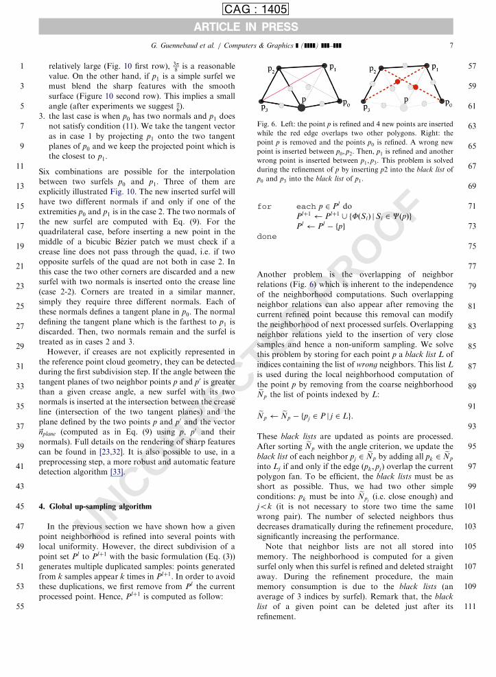
Fig. 8. A close view of the chameleon model (76k pts). Left:

EWA splatting. Right: after two refinement steps.

G. Guennebaud et al. / Computers & Graphics ] (]]]]) ]]]–]]]8

RREC

5. Real-time rendering

Our refinement procedure has been designed to

improve the rendering quality of point based geometry

in the context of real-time applications. It is efficiently

added on top of a hardware accelerated EWA splatting

algorithm [4,32] that allows holes filling and high

frequency filtering. Indeed it is too expensive and

unnecessary to up-sample the model until the size of

projected surfels is smaller than a single pixel. A

threshold value between two and four pixels is enough

for high quality visualization. Whereas our refinement

algorithm is fast, it is not conceivable to iteratively up-

sample the entire model at each frame. It is preferable to

up-sampled only parts of the model that need to be

refined and store the new geometry into a bounded

cache. We achieve this goal by dynamically updating an

octree.

According to the size of the input model, we can start

from a precomputed octree which contains coarse levels,

from a grid which can be immediately computed or from

a unique cell which contains the entire model. Classi-

cally, nodes of the octree are recursively processed by

performing simple visibility test and density estimation.

In addition, if a leaf is not dense enough then it becomes

a node and new leaves are created using our up-sampling

procedure. On the contrary, if an inserted node is out

dated (not rendered since a long time) then it is deleted

with all its children. The new points are inserted into a

pre-allocated chunk of memory, hence nodes store only

a range of indexes. So, owing to temporal and spatial

coherency, only a few nodes have to be refined at each

frame and real-time framerates are reached. We also

bound the length of the refinement procedure: if a

prefixed delay expires, we break the refinement process

and perform the rendering with the available data. The

remaining refinement process will be done at the next

frame. Since the splatting process can be entirely

performed by the graphics hardware, GPU and CPU

tasks can be efficiently organized. So, we recommend

that the rendering of available data starts before the up-

UNCO

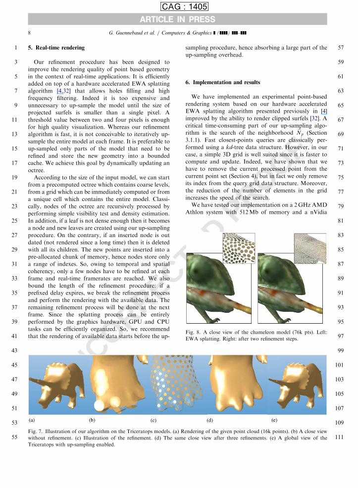
Fig. 7. Illustration of our algorithm on the Triceratops models. (a) R

without refinement. (c) Illustration of the refinement. (d) The same

Triceratops with up-sampling enabled.

sampling procedure, hence absorbing a large part of the

up-sampling overhead.

ROOF

6. Implementation and results

We have implemented an experimental point-based

rendering system based on our hardware accelerated

EWA splatting algorithm presented previously in [4]

improved by the ability to render clipped surfels [32]. A

critical time-consuming part of our up-sampling algo-

rithm is the search of the neighborhood eNp (Section

3.1.1). Fast closest-points queries are classically per-

formed using a kd-tree data structure. However, in our

case, a simple 3D grid is well suited since it is faster to

compute and update. Indeed, we have shown that we

have to remove the current processed point from the

current point set (Section 4), but in fact we only remove

its index from the query grid data structure. Moreover,

the reduction of the number of elements in the grid

increases the speed of the search.

We have tested our implementation on a 2GHz AMD

Athlon system with 512Mb of memory and a nVidia

99

101

103

105

107

109

111endering of the given point cloud (16k points). (b) A close view

close view after three refinements. (e) A global view of the

ORRECD P

ROOF

1

3

5

7

9

11

13

15

17

19

21

23

25

27

29

31

33

35

37

39

41

43

45

47

49

51

53

55

57

59

61

63

65

67

69

71

73

75

77

79

81

83

85

87

89

91

93

95

97

99

101

103

105

107

109

111

ARTICLE IN PRESSCAG : 1405

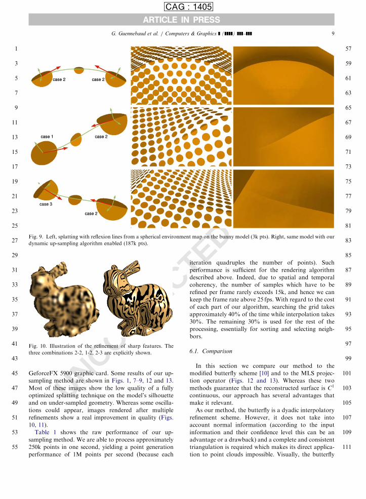
Fig. 9. Left, splatting with reflexion lines from a spherical environment map on the bunny model (3k pts). Right, same model with our

dynamic up-sampling algorithm enabled (187k pts).

Fig. 10. Illustration of the refinement of sharp features. The

three combinations 2-2, 1-2, 2-3 are explicitly shown.

G. Guennebaud et al. / Computers & Graphics ] (]]]]) ]]]–]]] 9

UNCGeforceFX 5900 graphic card. Some results of our up-

sampling method are shown in Figs. 1, 7–9, 12 and 13.

Most of these images show the low quality of a fully

optimized splatting technique on the model’s silhouette

and on under-sampled geometry. Whereas some oscilla-

tions could appear, images rendered after multiple

refinements show a real improvement in quality (Figs.

10, 11).

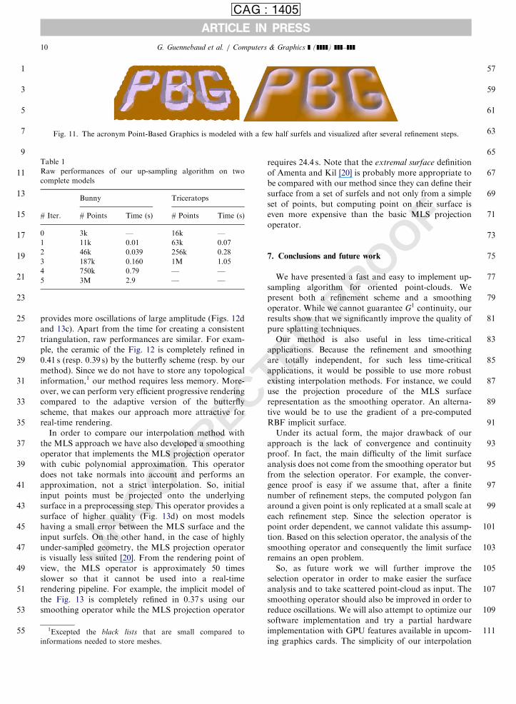
Table 1 shows the raw performance of our up-

sampling method. We are able to process approximately

250k points in one second, yielding a point generation

performance of 1M points per second (because each

TEiteration quadruples the number of points). Such

performance is sufficient for the rendering algorithm

described above. Indeed, due to spatial and temporal

coherency, the number of samples which have to be

refined per frame rarely exceeds 15k, and hence we can

keep the frame rate above 25 fps. With regard to the cost

of each part of our algorithm, searching the grid takes

approximately 40% of the time while interpolation takes

30%. The remaining 30% is used for the rest of the

processing, essentially for sorting and selecting neigh-

bors.

6.1. Comparison

In this section we compare our method to the

modified butterfly scheme [10] and to the MLS projec-

tion operator (Figs. 12 and 13). Whereas these two

methods guarantee that the reconstructed surface is C1

continuous, our approach has several advantages that

make it relevant.

As our method, the butterfly is a dyadic interpolatory

refinement scheme. However, it does not take into

account normal information (according to the input

information and their confidence level this can be an

advantage or a drawback) and a complete and consistent

triangulation is required which makes its direct applica-

tion to point clouds impossible. Visually, the butterfly

F

1

3

5

7

9

11

13

15

17

19

21

23

25

27

29

31

33

35

37

39

41

43

45

47

49

51

53

55

57

59

61

63

65

67

69

71

73

75

77

79

81

83

85

87

89

91

93

95

97

99

101

103

105

107

109

ARTICLE IN PRESSCAG : 1405

Fig. 11. The acronym Point-Based Graphics is modeled with a few half surfels and visualized after several refinement steps.

Table 1

Raw performances of our up-sampling algorithm on two

complete models

Bunny Triceratops

# Iter. # Points Time (s) # Points Time (s)

0 3k — 16k —

1 11k 0.01 63k 0.07

2 46k 0.039 256k 0.28

3 187k 0.160 1M 1.05

4 750k 0.79 — —

5 3M 2.9 — —

G. Guennebaud et al. / Computers & Graphics ] (]]]]) ]]]–]]]10

UNCORREC

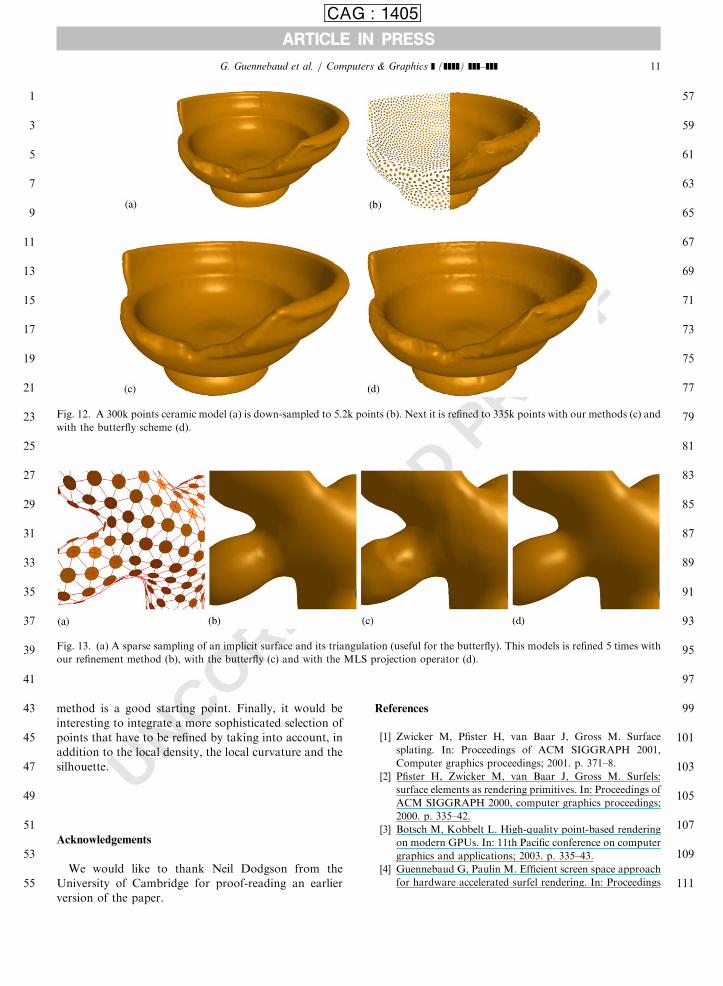
provides more oscillations of large amplitude (Figs. 12d

and 13c). Apart from the time for creating a consistent

triangulation, raw performances are similar. For exam-

ple, the ceramic of the Fig. 12 is completely refined in

0.41 s (resp. 0.39 s) by the butterfly scheme (resp. by our

method). Since we do not have to store any topological

information,1 our method requires less memory. More-

over, we can perform very efficient progressive rendering

compared to the adaptive version of the butterfly

scheme, that makes our approach more attractive for

real-time rendering.

In order to compare our interpolation method with

the MLS approach we have also developed a smoothing

operator that implements the MLS projection operator

with cubic polynomial approximation. This operator

does not take normals into account and performs an

approximation, not a strict interpolation. So, initial

input points must be projected onto the underlying

surface in a preprocessing step. This operator provides a

surface of higher quality (Fig. 13d) on most models

having a small error between the MLS surface and the

input surfels. On the other hand, in the case of highly

under-sampled geometry, the MLS projection operator

is visually less suited [20]. From the rendering point of

view, the MLS operator is approximately 50 times

slower so that it cannot be used into a real-time

rendering pipeline. For example, the implicit model of

the Fig. 13 is completely refined in 0.37 s using our

smoothing operator while the MLS projection operator

1Excepted the black lists that are small compared to

informations needed to store meshes.

requires 24.4 s. Note that the extremal surface definition

of Amenta and Kil [20] is probably more appropriate to

be compared with our method since they can define their

surface from a set of surfels and not only from a simple

set of points, but computing point on their surface is

even more expensive than the basic MLS projection

operator.

111

TED PROO7. Conclusions and future work

We have presented a fast and easy to implement up-

sampling algorithm for oriented point-clouds. We

present both a refinement scheme and a smoothing

operator. While we cannot guarantee G1 continuity, our

results show that we significantly improve the quality of

pure splatting techniques.

Our method is also useful in less time-critical

applications. Because the refinement and smoothing

are totally independent, for such less time-critical

applications, it would be possible to use more robust

existing interpolation methods. For instance, we could

use the projection procedure of the MLS surface

representation as the smoothing operator. An alterna-

tive would be to use the gradient of a pre-computed

RBF implicit surface.

Under its actual form, the major drawback of our

approach is the lack of convergence and continuity

proof. In fact, the main difficulty of the limit surface

analysis does not come from the smoothing operator but

from the selection operator. For example, the conver-

gence proof is easy if we assume that, after a finite

number of refinement steps, the computed polygon fan

around a given point is only replicated at a small scale at

each refinement step. Since the selection operator is

point order dependent, we cannot validate this assump-

tion. Based on this selection operator, the analysis of the

smoothing operator and consequently the limit surface

remains an open problem.

So, as future work we will further improve the

selection operator in order to make easier the surface

analysis and to take scattered point-cloud as input. The

smoothing operator should also be improved in order to

reduce oscillations. We will also attempt to optimize our

software implementation and try a partial hardware

implementation with GPU features available in upcom-

ing graphics cards. The simplicity of our interpolation

RRECTED PROOF

1

3

5

7

9

11

13

15

17

19

21

23

25

27

29

31

33

35

37

39

41

43

45

47

49

51

53

55

57

59

61

63

65

67

69

71

73

75

77

79

81

83

85

87

89

91

93

95

97

99

101

103

ARTICLE IN PRESSCAG : 1405

Fig. 12. A 300k points ceramic model (a) is down-sampled to 5.2k points (b). Next it is refined to 335k points with our methods (c) and

with the butterfly scheme (d).

Fig. 13. (a) A sparse sampling of an implicit surface and its triangulation (useful for the butterfly). This models is refined 5 times with

our refinement method (b), with the butterfly (c) and with the MLS projection operator (d).

G. Guennebaud et al. / Computers & Graphics ] (]]]]) ]]]–]]] 11

NCOmethod is a good starting point. Finally, it would be

interesting to integrate a more sophisticated selection of

points that have to be refined by taking into account, in

addition to the local density, the local curvature and the

silhouette.

U105

107

109

111

Acknowledgements

We would like to thank Neil Dodgson from the

University of Cambridge for proof-reading an earlier

version of the paper.

References

[1] Zwicker M, Pfister H, van Baar J, Gross M. Surface

splating. In: Proceedings of ACM SIGGRAPH 2001,

Computer graphics proceedings; 2001. p. 371–8.

[2] Pfister H, Zwicker M, van Baar J, Gross M. Surfels:

surface elements as rendering primitives. In: Proceedings of

ACM SIGGRAPH 2000, computer graphics proceedings;

2000. p. 335–42.

[3] Botsch M, Kobbelt L. High-quality point-based rendering

on modern GPUs. In: 11th Pacific conference on computer

graphics and applications; 2003. p. 335–43.

[4] Guennebaud G, Paulin M. Efficient screen space approach

for hardware accelerated surfel rendering. In: Proceedings

1

3

5

7

9

11

13

15

17

19

21

23

25

27

29

31

33

35

37

39

41

43

45

47

49

51

53

55

57

59

61

63

65

67

69

71

73

75

77

79

81

83

85

87

ARTICLE IN PRESSCAG : 1405

G. Guennebaud et al. / Computers & Graphics ] (]]]]) ]]]–]]]12

ORREC

of vision, modeling and visualization, IEEE signal proces-

sing society; 2003. p. 41–9.

[5] Clark EC. Recursively generated b-spline surfaces on

arbitrary topological meshes. Computer Aided Design

1978;10(6):350–5.

[6] Doo D, Sabin M. Analysis of the behaviour of recursive

subdivision surfaces near extraordinary points. Computer

Aided Design 1978;10(6):356–60.

[7] Zorin D, Schroder P. Subdivision for modeling and

animation. In: SIGGRAPH 2000 course notes, 2000.

[8] Warren J, Weimer H. Subdivision methods for geometric

design: a constructive approach, 2002.

[9] Dyn N, Levin D, Gregory J. A butterfly subdivision

scheme for surface interpolation with tension control.

ACM Transaction on Graphics 1990;9(2):160–9.

[10] Zorin D, Schroder P, Sweldens W. Interpolating subdivi-

sion for meshes with arbitrary topology. In: Proceedings of

ACM SIGGRAPH 1996, computer graphics proceedings;

1996. p. 189–92.

[11] Kobbelt L. Interpolatory subdivision on open quadrilat-

eral nets with arbitrary topology. In: Proceedings of

Eurographics; 1996.

[12] Hoppe H, DeRose T, Duchamp T, McDonald J, Stuezle

W. Surface reconstruction from unorganized points. In:

Proceedings of ACM SIGGRAPH 92, Computer graphics

proceedings; 1992.

[13] Carr JC, Beatson RK, Cherrie JB, Mitchell TJ, Fright

WR, McCallum BC, Evans TR. Reconstruction and

representation of 3D objects with radial basis functions.

In: Proceedings of ACM SIGGRAPH 2001, Computer

graphics proceedings; 2001. p. 67–76.

[14] Ohtake Y, Belyaev A, Alexa M, Turk G, Seidel H-P.

Multi-level partition of unity implicits. ACM Transactions

on Graphics 2003;22(3):463–70.

[15] Tobor I, Reuter P, Schlick C. Multiresolution reconstruc-

tion of implicit surfaces with attributes from large

unorganized point sets. In: Proceedings of shape modeling

international; 2004.

[16] Levin D. Mesh-independent surface interpolation. In:

Advances in computational mathematics; 2001.

[17] Adamson A, Alexa M. Approximating and intersecting

surfaces from points. In: Proceedings of the Eurographics

symposium on geometry processing; 2003. p. 245–54.

[18] Adamson A, Alexa M. Approximating bounded, non-

orientable surfaces from points. In: Proceedings of shape

modeling international; 2004.

[19] Alexa M, Adamson A. On normals and projection

operators for surfaces defined by point sets. In: Proceed-

UN

TED PROOF

ings of the eurographics symposium on point-based

graphics; 2004. p. 149–55.

[20] Amenta N, Kil YJ. Defining point set surfaces. In:

Proceedings of ACM SIGGRAPH 2004, Computer

graphics proceedings, 2004, to appear.

[21] Alexa M, Behr J, Cohen-Or D, Fleishman S, Levin D,

Silva CT. Computing and rendering point set surface.

IEEE Transaction on Visualization and Computer Gra-

phics 2003;9(1):3–15.

[22] Pauly M, Gross M, Kobbelt LP. Efficient simplification of

point-sampled surfaces. In: Proceedings of the 13th IEEE

visualization conference; 2002. p. 163–70.

[23] Pauly M, Keiser R, Kobbelt LP, Gross M. Shape modeling

with point-sampled geometry. In: Proceedings of ACM

SIGRAPH 2003, Computer graphics proceedings; 2003. p.

641–50.

[24] Turk G. Re-tiling polygonal surface. In: Proceedings of

ACM SIGGRAPH 92, computer graphics proceedings;

1992.

[25] Stamminger M, Drettakis G. Interactive sampling and

rendering for complex and procedural geometry. In:

Proceedings of the 12th eurographics workshop on

rendering; 2001. p. 151–62.

[26] Guennebaud G, Barthe L, Paulin M. Real-time point

cloud refinement. In: Proceedings of Eurographics sympo-

sium on point-based graphics; 2004. p. 41–8.

[27] Linsen L, Prautzsch H. Fan clouds—an alternative to

meshes. In: Dagstuhl seminar 02151 on theoretical

foundations of computer vision—geometry, morphology,

and computational imaging, 2002.

[28] Floater MS, Reimers M. Meshless parameterization and

surface reconstruction. Computer Aided Geometric De-

sign 2001;18:77–92.

[29] Vlachos A, Peters J, Boyd C, Mitchell JL. Curved PN

triangles. In: Proceedings of the 2001 symposium on

interactive 3D graphics; 2001.

[30] Farin G. CAGD a practical guide, 5th ed. New York:

Academic Press; 2002.

[31] van Overveld CWAM, Wyvill B. Phong normal interpola-

tion revisited. ACM Transaction on Graphics

1997;16(4):397–419.

[32] Zwicker M, Rasanen J, Botsch M, Dachsbacher C, Pauly

M. Perspective accurate splatting. In: Graphics interface,

2004, to appear.

[33] Pauly M, Keiser R, Gross M. Multi-scale feature extrac-

tion on point-sampled models. In: Proceedings of euro-

graphics; 2003. p. 121–30.

C