1

Dynamic response of earlywood and latewood within annual growth ring

structure of Scots pine subjected to changing relative humidity

Leszek Krzemień1, Marcin Strojecki1,*, Sebastian Wroński2, Jacek Tarasiuk2 and Michał

Łukomski1

1Jerzy Haber Institute of Catalysis and Surface Chemistry, Polish Academy of Sciences, Kraków,

Poland

2Faculty of Physics and Applied Computer Science, AGH - University of Science and

Technology, Kraków, Poland

*Corresponding author

Jerzy Haber Institute of Catalysis and Surface Chemistry, Polish Academy of Sciences, ul.

Niezapominajek 8, 30-239 Kraków, Poland

Phone: +48-12-6395119

E-mail: ncstroje@cyf-kr.edu.pl

Abstract: Scots pine (Pinus sylvestris L.) was subjected to relative humidity (RH) changes and

the dynamic strain field on the surface and in the bulk wood was monitored by digital speckle

pattern interferometry (DSPI) and X-ray computed microtomography (μXCT) assisted by digital

volume correlation (DVC). If a freely shrinking specimen was subjected to an RH decrement,

earlywood (EW) and latewood (LW) at the surface layer were deformed in the opposite

directions at the beginning of drying due to moisture gradient across the specimen. As a result,

the surface and core behaved as independent sub-components, with the surface restrained in its

response by the dimensionally unchanged core. With time, both LW and EW shrank as moisture

content (MC) became uniform across the specimen. When an entire wood specimen was

restrained from movement and desiccated in ambient RH, EW was stretched to compensate for

the considerable shrinkage of LW. Knowledge about surface deformation at the annual ring level

as a function of varying RH may be helpful to assess the risks associated with the damage of

paint layers caused by fluctuations of ambient RH.

Keywords: digital speckle pattern interferometry; dynamic moisture response; earlywood;

latewood; pine wood; X-ray computed microtomography;

2

Introduction

Cracks in paint layers on wood exhibit a clear correlation with growth ring structure. The

interrelation between wood structure and paint layer cracking has several implications, such as

for furniture manufacturers and for conservators striving to prevent moisture-induced damage in

diverse objects of fine and applied arts, such as panel paintings, furniture or polychrome

sculpture (Keck 1969; Mecklenburg et al. 1998). It is also known that formation of cracks on

wood exposed to harsh climatic conditions is related to growth rings (Williams 1999).

Wood has a complex hierarchical structure resulting from the characteristic orientation of

microfibrils (MFs) in the cell wall layers and the alternation of earlywood (EW) and latewood

(LW) in annual growth rings with different cell wall thicknesses and densities in each of the

tissues. This is the reason why the moisture-induced swelling is different in the three principal

anatomical directions (anisotropy). The swelling anisotropy is not well understood at the micro-

scale of wood cells and tissues regardless of the research in the last decade.

Murata and Masuda (2001, 2006) determined the microscopic swelling behaviour of LW

tracheids in Douglas fir by confocal laser scanning microscopy (CLSM) and digital image

correlation (DIC). Moisture-related swelling was found to be the same in radial (R) and tangential

(T) directions. The authors concluded, therefore, that the swelling anisotropy of large wood

specimens must derive from the interaction between EW and LW. This conclusion was

confirmed by subsequent studies. Derome et al. (2011) induced moisture swelling of Norway

spruce (Picea abies L.) by gradual changes in relative humidity (RH) and observed the effects at

the cellular scale by high-resolution X-ray tomographic microscopy (µXCT). Specimens of EW

and LW (0.5 mm thick) were measured separately. The relationship between the dimensional

change and RH was close to linear, between 25 and 85% RH. The dimensional change

coefficients determined in the R direction across that range were 0.04% per 1% RH (shortly

3

% RH−1) and 0.011% RH−1 in LW and EW, respectively. In contrast, the difference in the T

swelling of LW and EW was not significant with coefficients being 0.045 and 0.038% RH−1,

respectively. Lower R swelling of EW was explained by a lower amount of moisture adsorbed in

the EW cell walls and a strong restraint of rays in that direction, while the restraining effect is

less pronounced in LW due to its higher stiffness.

Much smaller moisture-induced R swelling of EW was confirmed in the microscopic

studies of swelling behaviour of the bulk Norway spruce, performed by DIC (Keunecke et al.

2012; Lanvermann et al. 2013). Authors of the latter study demonstrated that the R swelling

coefficient for LW was 0.25% per 1% moisture content (shortly % MC-1) or approximately

0.05% RH-1, when compared to 0.07% MC-1 (or 0.015% RH-1) for EW. With the equal T

swelling coefficients for LW and EW (0.33% MC-1 or 0.07% RH-1), it was demonstrated that the

anisotropic hygric behaviour of wood is solely governed by restrained swelling in the R direction.

The experimental full field measurements of moisture-induced strains agreed remarkably

well with the mechanical and swelling behaviour at growth ring level predicted by a multiscale

finite element model based on microstructural information concerning the geometry of the wood

cells, local density, MF angle, mechanical and swelling properties of cell wall layers (Rafsanjani

et al. 2013). The highly non-uniform R strain profiles strictly followed the density profiles across

the growth ring structure and the T strain profiles were uniform. The model revealed that the

uniformity of T-profiles is due to the similar swelling of EW and LW in the T direction and the

high stiffness of LW, which forces EW into T tension and this leads to expanding tissues in that

direction in the same extent.

LW is denser than EW, and this non uniformity accounts for the variation of stiffness

over the growth ring scale. EW deforms 1.5 times more than LW in spruce, when a

4

macroscopic wood element is under R compression (Garab 2010). The change in the

elasticity modulus in the R direction of Norway spruce was from 671 to 1570 MPa over a

single growth ring (Persson et al. 2000). Moisture-related dimensional changes within

growth rings have so far focused on the static situation, in which wood is in an equilibrium

state with ambient RH and localized dimensional changes attain constant levels.

However, the dynamic response of the complex structure of wood to RH changes is of

fundamental interest, as temporal strain fields across wood could be different from that in the

equilibrium state. The wood deformation at the micro level – on the surface and in the bulk

material – can effectively be observed by digital speckle pattern interferometry (DSPI) and μXCT

aided by DVC (Umezaki et al. 2004; Müller et al. 2005; Valla et al. 2011; Forsberg et al. 2010).

Recently, the usefulness of µXCT applied to the measurement of shrinkage in beech wood was

reported by Taylor et al. (2013). This is the reason why, in the present study, the dynamic

shrinkage of wood was observed at the micro level by combination of DSPI and µXCT and DVC

as instruments.

Materials and methods

A 10(T) x 10(L) x 15(R) mm specimen of Scots pine (Pinus sylvestris) wood was machined from

a dried and seasoned clear part of a trunk. Prior to the measurements, the specimen was

conditioned at 75% RH over a week to stabilize its dimensions in a swollen state. The

equilibrium moisture content (EMC) in the specimen (14%) was calculated as the average of

corresponding MC values on the adsorption and desorption branches of the sorption isotherm

(Bratasz et al. 2012). The same approach was used throughout the paper. Two sides of the

specimen perpendicular to wood fibres were sealed with silicone to enable the diffusion of water

5

vapour along the R and T directions only. In this way, the same situation was created as in typical

wooden objects, which are much longer and wider than they are thick.

In the surface oriented experiments, the strain field on the surface was continuously

monitored by means of a home-made 1D in-plane DSPI. The instrument setup is powered by a

Samba 300~mW frequency doubled Nd:YAG single mode laser from Cobolt (Cobolt AB, Solna,

Sweden). The beam is split into two paths by a non-polarizing beam splitter cube and expanded

to 40 mm in diameter. In one arm of the interferometer, a mirror is mounted on a piezoelectric

phase shifter. This allows an arbitrary phase difference between the beams to be introduced,

which is needed as a four frame phase stepping algorithm along with the spatial phase

unwrapping is used to obtain information about displacements, as described in Rastogi’s book

(2000).

The images were taken by means of a BCi4-6600 CCD camera (C-cam Technologies,

Vector international bvba, Leuven, Belgium; 6.6 MPixel; 2208 x 3000 pixels) every minute after

an abrupt RH decrement from 75 to 50%. The DSPI experiments were conducted for free and

restrained shrinkage. In the first case, one end of the specimen was clamped in a vice and the

other end, observed by the CCD camera, could swell freely. In the second case, both specimens’

ends were fixed in the vice. The RH in the laboratory was stabilised by means of humidifiers and

in the home-built climatic box, in which both the DSPI setup and the specimen were enclosed, a

bentonite clay dessicant (Desi Pack) was placed with a huge moisture capacity (conditioned at

50% of RH).

In the second type of experiment, the strain field inside the same specimen was measured in

time intervals by μXCT (180N from GE Sensing & Inspection Technologies phoenix | X-ray

Gmbh, Munich, Germany). The machine was equipped with a nanofocus X-ray tube (V=100 kV

and I = 200 µA). The tomograms were recorded on a Hamamatsu (HAM C 7942CA-02,

6

Hamamatsu Photonics K.K., Hamamatsu,Japan) 2300 x 2300 pixel detector. During the

measurement, a tungsten target was used. 1400 projections were taken with an exposure time of

500 ms with 3 integrations for each exposition. The total time of measurement was around 40

min. The reconstruction of measured objects was done with the aid of proprietary GE software

(datosX ver. 2.1.0) in combination with the Feldkamp algorithm for a cone beam X-ray CT

(Feldkamp et.al. 1984). The post reconstruction of data was performed by means of VGStudio

Max 2.1 (Volume Graphics GmbH, Heidelberg, Germany) (Reference Manual 2013).

The whole measured volume of the specimen was 10(T) x 9(L) x 15(R) mm3, whereas the

final resolution of the reconstructed object was 6.75 µm. Such a reduced resolution was adequate

for further calculations but, on the other hand, allowed for relatively short time of data

acquisition, which allowed the minimization of the blurring effect due to the shrinkage of the

specimen during the experiment.

Tomograms were taken at 3, 13, and 76 h after an abrupt RH decrement from 75 to 40%.

The DVC method was implemented into the MATLAB (The MathWorks, Inc., MA, USA) code

developed by the authors to calculate the strain field inside the volume of the measured specimen.

Digital volume correlation is usually performed in the 2D digital image correlation (2D

DIC) mode (Peters and Ranson 1982). However, in such method, the pseudo-strains cannot be

eliminated, which are caused by out-of- plane displacement occurring during the specimen’s

deformation. Therefore, a 3D DVC was developed to analyse μXCT images. DVC is a

computational method applied to images recorded prior to and after the deformation of an object

leading to 3D deformation fields. The original approach of Bay et al. (1999) was modified by a

number of researchers ( Forsberg et al.2010 ; Gates and Lambros 2013 ) and very recently a

commercial DVC has been created as part of lavisoion strainmaster software. The technique

consists of finding a mathematical transformation, which correlates images before and after

7

deformation. An alignment of images is defined on the basis of least squares or a cross-

correlation criterion for selected features. The whole volume of the object is divided into small

sub-volumes, for which calculations are performed independently. Thus voxel images are

obtained by the interpolation of the calculation results. Regardless of the type of criterion selected

for pattern-matching, the DVC algorithm is always based on an optimisation of the

transformation function, so the choice of the function type and its initial parameters is essential

(Gates and Lambros 2013). After the pattern-matching procedure, the obtained transformation

parameters need to be recalculated into displacement and strain fields. The whole procedure

involves three phases.

1. Initial aligning. Prior to dividing the volume of the object into small sub-volumes, the

parameters of affine transformation (a combination of linear deformation and rotation) and

translation are calculated in order to align a few, manually selected features on images captured

before and after the deformation. This initial phase of the calculations assures consistency of the

DVC procedure in the case of deformations larger than 10 voxels. In the algorithm applied in this

study, the affine transformation matrix A and translation vector T are determined in the procedure

of aligning the position of four pairs of voxels selected by the user. Results are obtained by

solving the following set of equations:

where Vi and V’i are vectors indicating the position of the i-th of four voxels before and after the

deformation, respectively. Once matrix A and vector T are determined, the image of the

deformed specimen is transformed using Matlab Image Processing Toolbox library. At the end of

this stage of calculations, parameters of transformation leading to the coarse alignment of the

object before and after the deformation are obtained.

8

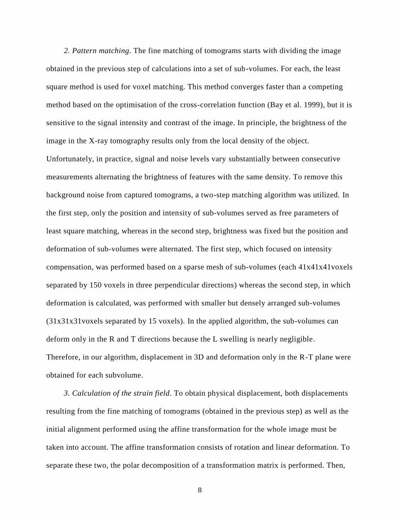
2. Pattern matching. The fine matching of tomograms starts with dividing the image

obtained in the previous step of calculations into a set of sub-volumes. For each, the least

square method is used for voxel matching. This method converges faster than a competing

method based on the optimisation of the cross-correlation function (Bay et al. 1999), but it is

sensitive to the signal intensity and contrast of the image. In principle, the brightness of the

image in the X-ray tomography results only from the local density of the object.

Unfortunately, in practice, signal and noise levels vary substantially between consecutive

measurements alternating the brightness of features with the same density. To remove this

background noise from captured tomograms, a two-step matching algorithm was utilized. In

the first step, only the position and intensity of sub-volumes served as free parameters of

least square matching, whereas in the second step, brightness was fixed but the position and

deformation of sub-volumes were alternated. The first step, which focused on intensity

compensation, was performed based on a sparse mesh of sub-volumes (each 41x41x41voxels

separated by 150 voxels in three perpendicular directions) whereas the second step, in which

deformation is calculated, was performed with smaller but densely arranged sub-volumes

(31x31x31voxels separated by 15 voxels). In the applied algorithm, the sub-volumes can

deform only in the R and T directions because the L swelling is nearly negligible.

Therefore, in our algorithm, displacement in 3D and deformation only in the R-T plane were

obtained for each subvolume.

3. Calculation of the strain field. To obtain physical displacement, both displacements

resulting from the fine matching of tomograms (obtained in the previous step) as well as the

initial alignment performed using the affine transformation for the whole image must be

taken into account. The affine transformation consists of rotation and linear deformation. To

separate these two, the polar decomposition of a transformation matrix is performed. Then,

9

only a Hermitian part of the matrix, describing deformation, is needed to correct the

displacement field obtained from the sub-volumes matching procedure.

In this paper, only R strain fields will be presented. The R derivative of the R displacement

was calculated by convolving the image with an appropriately normalised derivative of the

Gaussian function as described in Tomasi (2003).

Results and discussion

Freely shrinking specimen

In-plane DSPI measurements of time evolution of the surface strain were performed for an

unrestrained radially cut pine specimen conditioned at 75% RH (14% MC) and subjected to an

abrupt RH decrement to 50% (10% MC). The results are shown in Fig. 1. The dimension of the

specimen altered over the analyzed time period. Both EW and LW shrank after 30 h when the

wood reached about half its equilibrium length, which is in agreement with the numerical

calculations by Rachwał et al. (2012). However, at the very beginning of the RH change, the

strains of EW and LW were opposite. The effect is further illustrated in Fig. 2.

The reversal of strain sign for EW during the first few hours after the change in RH can be

explained by internal restraint due to uneven moisture distribution in the specimen. Due to the

limited speed of moisture diffusion at the beginning of the RH change, the core of the specimen

did not experience change in the MC, and hence did not change dimensionally. The immediate

dimensional response occurred to RH decrement in the environment, however, only on the

wood’s surface. The surface response was restrained by the dimensionally stable core. As a

result, the surface and core behaved as independent sub-components, hence during the first 30

min the former behaved like a restrained specimen. Indeed, the strain of the LW seems to be

10

unperturbed by the internal restrain in the early phase of drying. With time, both LW and EW

shrank as the MC became uniform across the specimen.

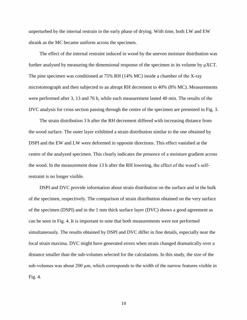
The effect of the internal restraint induced in wood by the uneven moisture distribution was

further analysed by measuring the dimensional response of the specimen in its volume by µXCT.

The pine specimen was conditioned at 75% RH (14% MC) inside a chamber of the X-ray

microtomograph and then subjected to an abrupt RH decrement to 40% (8% MC). Measurements

were performed after 3, 13 and 76 h, while each measurement lasted 40 min. The results of the

DVC analysis for cross section passing through the centre of the specimen are presented in Fig. 3.

The strain distribution 3 h after the RH decrement differed with increasing distance from

the wood surface. The outer layer exhibited a strain distribution similar to the one obtained by

DSPI and the EW and LW were deformed in opposite directions. This effect vanished at the

centre of the analyzed specimen. This clearly indicates the presence of a moisture gradient across

the wood. In the measurement done 13 h after the RH lowering, the effect of the wood’s self-

restraint is no longer visible.

DSPI and DVC provide information about strain distribution on the surface and in the bulk

of the specimen, respectively. The comparison of strain distribution obtained on the very surface

of the specimen (DSPI) and in the 1 mm thick surface layer (DVC) shows a good agreement as

can be seen in Fig. 4. It is important to note that both measurements were not performed

simultaneously. The results obtained by DSPI and DVC differ in fine details, especially near the

local strain maxima. DVC might have generated errors when strain changed dramatically over a

distance smaller than the sub-volumes selected for the calculations. In this study, the size of the

sub-volumes was about 200 µm, which corresponds to the width of the narrow features visible in

Fig. 4.

11

Restrained specimen

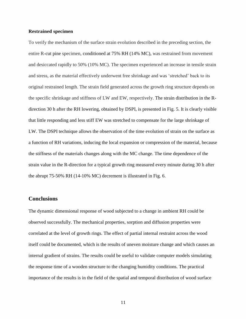
To verify the mechanism of the surface strain evolution described in the preceding section, the

entire R-cut pine specimen, conditioned at 75% RH (14% MC), was restrained from movement

and desiccated rapidly to 50% (10% MC). The specimen experienced an increase in tensile strain

and stress, as the material effectively underwent free shrinkage and was ‘stretched’ back to its

original restrained length. The strain field generated across the growth ring structure depends on

the specific shrinkage and stiffness of LW and EW, respectively. The strain distribution in the R-

direction 30 h after the RH lowering, obtained by DSPI, is presented in Fig. 5. It is clearly visible

that little responding and less stiff EW was stretched to compensate for the large shrinkage of

LW. The DSPI technique allows the observation of the time evolution of strain on the surface as

a function of RH variations, inducing the local expansion or compression of the material, because

the stiffness of the materials changes along with the MC change. The time dependence of the

strain value in the R-direction for a typical growth ring measured every minute during 30 h after

the abrupt 75-50% RH (14-10% MC) decrement is illustrated in Fig. 6.

Conclusions

The dynamic dimensional response of wood subjected to a change in ambient RH could be

observed successfully. The mechanical properties, sorption and diffusion properties were

correlated at the level of growth rings. The effect of partial internal restraint across the wood

itself could be documented, which is the results of uneven moisture change and which causes an

internal gradient of strains. The results could be useful to validate computer models simulating

the response time of a wooden structure to the changing humidity conditions. The practical

importance of the results is in the field of the spatial and temporal distribution of wood surface

12

deformation under varying RH conditions. The effect is especially important for short-term RH

fluctuations, for which the mutual interaction of EW and LW produces local strains at the surface

layer, which are higher than the average response of the macroscopic sample. Thus the risks can

be better assessed, which are associated with the damage of paint layers caused by fluctuations of

ambient RH. The experimental techniques – DSPI and μXCT assisted by DVC analysis – are

very useful for monitoring dynamic strain fields on the surface and in the bulk of wood

specimens subjected to RH change. The deformations of wooden samples monitored by the

µXCT can be analysed quantitatively by the elaborated DVC method. The only situations in

which the DVC algorithm fails is, when the strain changes dramatically over a distance smaller

than the sub-volumes selected for the calculations.

Acknowledgements: This research received funding from the Marian Smoluchowski

Krakow Research Consortium, a Leading National Research Centre (KNOW) supported by the

Ministry of Science and Higher Education. Further support by Grant UMO-

2011/01/B/HS2/02586 funded by the Polish National Science Centre is acknowledged.

References

Bay, B. K., Smith, T. S., Fyhrie, D. P., Saad, M. (1999) Digital volume correlation: three-

dimensional strain mapping using X-ray tomography. Exp. Mechanics 39:217-226.

Bratasz, Ł. Kozłowska, A., Kozłowski, R. (2012) Analysis of water adsorption by wood

using the Guggenheim-Anderson-de Boer equation. Eur. J. Wood Prod. 70:445–451.

Derome, D., Griffa, M., Koebel, M., Carmeliet, J. (2011) Hysteretic swelling of wood at cellular

scale probed by phase-contrast X-ray tomography. J. Struct. Biol. 173:180-190.

Feldkamp, L.A., Davis L.C., Kress J.W. (1984) Practical cone-beam algorithm. J. Opt. Soc. Am.

A1: 612-619.

Forsberg, F., Sjödahl, M., Mooser, R., Hack, E., Wyss, P. (2010) Full three-dimensional strain

measurements on wood exposed to three-point bending: analysis by use of digital volume

correlation applied to synchrotron radiation micro-computed tomography image data. Strain

46:47-60.

13

Garab, J., Keunecke, D., Hering, S., Szalai, J., Niemz, P. (2010) Measurement of standard and

off-axis elastic moduli and Poisson’s ratios of spruce and yew wood in the transverse plane.

Wood Sci. Technol. 44:451-464.

Gates, M., Lambros, J. High Performance Digital Volume Correlation, Springer, New York, pp.

307-314 (2013).

Keck, S. (1969). Mechanical alteration of the paint film. Studies in Conservation 14:9-30.

Keunecke, D., Novosseletz, K., Lanvermann, C., Mannes, D., Niemz, P. (2012) Combination of

X-ray and digital image correlation for the analysis of moisture-induced strain in wood:

opportunities and challenges. Eur. J. Wood. Prod. 70:407-413.

Lanvermann, C., Wittel, F. K., Niemz, P. (2013) Full-field moisture induced deformation in

Norway spruce: intra-ring variation of transverse swelling. Eur. J. Wood. Prod. 72:43-52.

Mecklenburg, M.F., Tumosa, C.S., Erhardt, D. (1998) Structural Response of Painted Wood

Surfaces to Changes in Ambient Relative Humidity. In: Painted Wood: History and

Conservation. Eds. Dorge, V., Howlett, F.C. The Getty Conservation Institute, Los Angeles,

pp. 464–83.

Murata, K., Masuda, K. (2001) Observation of microscopic swelling behaviour of the cell wall. J.

Wood Sci. 47:507-509.

Murata, K., Masuda, K. (2006) Microscopic observation of transverse swelling of latewood

tracheid: effect of macroscopic/mesoscopic structure. J. Wood Sci. 52:283-289.

Müller, U., Sretenovic, A., Vincenti, A., Gindl, W. (2005) Direct measurement of strain

distribution along a wood bond line. Part 1: Shear strain concentration in a lap joint

specimen by means of electronic speckle pattern interferometry. Holzforschung 59:300-

306.

Peters, W. H., Ranson, W. F. (1982) Digital imaging techniques in experimental stress analysis.

Optical Eng. 21:213427-213427.

Persson, K. Micromechanical modelling of wood and fibre properties. Lund University,

Department of Mechanics and Materials, Lund, 2000.

Rachwał, B., Bratasz, Ł., Łukomski, M., Kozłowski, R. (2012). Response of wood supports in

panel paintings subjected to changing climate conditions. Strain 48(5):366-374.

Rafsanjani, A., Lanvermann, C., Niemz, P., Carmeliet, J., Derome, D. (2013) Multiscale analysis

of free swelling of Norway spruce. Composites A 54:70-78.

Rastogi, P. K. (2000). Digital speckle pattern interferometry and related techniques. Digital

Speckle Pattern Interferometry and Related Techniques, by PK Rastogi (Editor), pp. 384.

Wiley-VCH, December 2000, 1.

Reference Manual VGStudio Max Release 2.0., Volume Graphics GmbH, 2013

http://www.volumegraphics.com/en/products/vgstudio-max.

Taylor, A., Plank, B., Standfest, G., Petutschnigg, A. (2013) Beech wood shrinkage observed at

the micro-scale by a time series of X-ray computed tomographs (μXCT). Holzforschung

67:201-205.

Tomasi, C. (2006) Convolution, smooting, and image derivatives. In: Introduction to computer

vision. Duke University Course.

Umezaki, E., Suzuki, T., Takahashi, M. (2004) Measurement of deformation of wood joints using

Electronic Speckle Pattern Interferometry. JSME Int. J. Series A 47: 274-279.

Valla, A., Konnerth, J., Keunecke, D., Niemz, P., Müller, U., Gindl, W. (2011) Comparison of

two optical methods for contactless, full field and highly sensitive in-plane deformation

measurements using the example of plywood. Wood Sci. Tech. 45:755-765.

14

Williams, R., S. (1999) Finishing of wood. In: Wood handbook. Wood as an engineering

material. Forest Products Laboratory, Department of Agriculture, Forest Service, US, pp

15/1–15/37.

15

LEGEND OF FIGURES

1. Radial strain distribution on the surface of a freely shrinking specimen 30 h after a 75-50%

RH decrement; a) picture of the specimen, b), c), and d) strain distribution after 30 min, 12

and 24 h, respectively, e) strain after 30 min, 12 and 24 h integrated parallel to the annual

growth rings.

2. The surface strain development of a freely shrinking specimen after a 75-50% RH decrement.

3. Radial strain distribution in the central section of the freely shrinking specimen, 3, 13 and 76 h

after a 75 - 40% RH decrement. Rectangles on the image indicate the areas of the plotted

strain.

4. Comparison of the radial strain distributions obtained by DSPI (solid black) and DVC (dashed

red). From top to bottom: The strain distribution after 3, 13 and 76 h after RH decrement.

5. Radial strain distribution on the surface of the restrained specimen, 30 h after a 75-50% RH

decrement. a) picture of the specimen, b) strain distribution, c) strain integrated parallel to the

growth rings.

6. Maximum negative (shrinkage) and positive (elongation) strain values in the radial direction

for the restrained and unrestrained specimen measured every minute during 30 h after a 75-

50% RH decrement.

16

0 2 4 6 8 10 12 14 16

-1.2

-1.0

-0.8

-0.6

-0.4

-0.2

0.0

0.2

e)

d)

c)

b)

Str

ain

(%

)

Radial distance (mm)

30 m

12 h

24 h

-0.005 Strain rate (%·min–1

) 0.005

a)

Fig. 1

17

0 4 8 12 16 20 24 28 32

-1.2

-1.0

-0.8

-0.6

-0.4

-0.2

0.0

0.2

average

earlywood

latewood

Str

ain

(%

)

Time (hours)

Fig. 2

0 1 2 3 4 5 6 7

-1.0

-0.8

-0.6

-0.4

-0.2

0.0

0.2

latewoodearlywood

earlywood latewood

3 h

13 h

76 h

Str

ain

(%

)

Tangential distance (mm)

earlywood

latewood

3h 13h 76h

Fig. 3

18

0.0

0.5

1.0

3h

Str

ain

(%

)

0.0

1.0

2.0

13h

S

tra

in (

%)

12 13 14 15 16 17 18 19 20 21 22

0.0

1.0

2.0 76h

Str

ain

(%

)

Radial distance (mm)

Fig. 4

0 2 4 6 8 10 12 14 16 18 20 22-0.8

-0.6

-0.4

-0.2

0.0

0.2

0.4

0.6

c)

b)

Str

ain

(%

)

Radial distance (mm)

0.5 Strain (%) -0.5

a)

Fig. 5

19

0 4 8 12 16 20 24 28 32

-1.6

-1.4

-1.2

-1.0

-0.8

-0.6

-0.4

-0.2

0.0

0.2

0.4

free restrained

average

earlywood

latewood

Str

ain

(%

)

Time (hours)

Fig. 6