A

toa

Aviovs©

K

1

e1hg2PV

f

(

0

BioSystems 91 (2008) 51–68

Available online at www.sciencedirect.com

Dynamic properties of a delayed protein cross talk model

Svetoslav Nikolov a, Julio Vera b, Vladimir Kotev a,Olaf Wolkenhauer b,∗, Valko Petrov a

a Institute of Mechanics and Biomechanics-BAS, Acad. G. Bonchev Str., Bl. 4, 1113 Sofia, Bulgariab Systems Biology and Bioinformatics Group, Department of Computer Science, University of Rostock, 18051 Rostock, Germany

Received 2 February 2007; received in revised form 3 July 2007; accepted 4 July 2007

bstract

In this paper we investigate how the inclusion of time delay alters the dynamical properties of the Jacob–Monod model, describinghe control of the �-galactosidase synthesis by the lac repressor protein in E. coli. The consequences of a time delay on the dynamicsf this system are analysed using Hopf’s theorem and Lyapunov–Andronov’s theory applied to the original mathematical modelnd to an approximated version.

Our analytical calculations predict that time delay acts as a key bifurcation parameter. This is confirmed by numerical simulations.critical value of time delay, which depends on the values of the model parameters, is analytically established. Around this critical

alue, the properties of the system change drastically, allowing under certain conditions the emergence of stable limit cycles, that

s self-sustained oscillations. In addition, the features of the end product repression play an essential role in the characterisationf these limit cycles: if cooperativity is considered in the end product repression, time delay higher than the mentioned criticalalue induce differentiated responses during the oscillations, provoking cycles of all-or-nothing response in the concentration of thepecies.

2007 Elsevier Ireland Ltd. All rights reserved.

ogy

eywords: Cross talk; Time delay; Bifurcation analysis; Systems biol

. Introduction

The process of translating observed data into a math-matical model is called dynamic modelling (Beltrami,987). Dynamical modelling of intracellular networksas emerged as a valuable tool for experimental data inte-ration and validation of biological hypotheses (Kolch,

000; Galach, 2003; Eungdamrong and Iyengar, 2004;etrov et al., 2005; Nikolov et al., 2005, 2006 andera et al., 2007a,b). Mathematical models have been

∗ Corresponding author. Tel.: +49 381 498 75 70;ax: +49 381 498 75 72.

E-mail address: olaf.wolkenhauer@informatik.uni-rostock.deO. Wolkenhauer).

URL: http://www.sbi.uni-rostock.de (O. Wolkenhauer).

303-2647/$ – see front matter © 2007 Elsevier Ireland Ltd. All rights reservdoi:10.1016/j.biosystems.2007.07.004

used to investigate the role of phosphorylation, multi-merisation, positive or negative feedback regulation oftranscription factors (Goldbeter, 1995; Smolen et al.,1998; Chen and Aihara, 2002; Salazar and Hofer, 2006),and gene expression multistability (Wolf and Eeckman,1998).

Time delay emerges in some cases as a constitutiveproperty of pathways (Timmer et al., 2004). The natureof time delay in biochemical system models is twofold.In some cases the time delay is related to processes thattake an intrinsic discrete time to be accomplished (forinstance, the synthesis of mRNA), while in other cases

it is a consequence of the modelling approach used,in which complex sequences of events, not representedin detail, provoke the emergence of an apparent timedelay. The processes related to gene expression induce

ed.

oSystem

52 S. Nikolov et al. / Bi

very often time delays in the biochemical systems.Smolen et al. (1999) describes a time delay associatedto the translocation of proteins and mRNAs between50 and 100 min. Rateitschak and Wolkenhauer (2007)describes a time delay for gene transcription between10 and 40 min. Finally, in Swameye et al. (2003) atime delay around 7 min is defined and estimated fornucleocytoplasmic shuttling, which describes the delayassociated to a pool of processes not described in detailin the model. Various authors have previously consid-ered biochemical oscillators with time delay (Nikolovet al., 2006) and the usefulness of bifurcation analysisto investigate properties of time-delay biochemical net-works (Rateitschak and Wolkenhauer, 2007; Mocek etal., 2005). Their analyses show that the introduction ofa large enough time delay can sometimes change theunique equilibrium of the system and induce periodicsolutions (self-oscillation), which arise from the equi-librium through an Andronov–Hopf bifurcation.

The use of the theory of dynamical systems for theinvestigation of pathologies relates to the concept of“dynamical diseases” (Glass and Mackey, 1988), whichdefines an anomalous temporal organisation emergingfrom a phatological configuration of the biochemicalsystem investigated. There are three main abnormal con-ditions that could emerge as consequence of a dynamicalpathology: (i) proteins or metabolic levels that showshomeostasis in normal conditions can lead to highamplitude periodical oscillations (Pigolotti et al., 2007);(ii) new periodicities with different time duration mayappear in biochemical systems that already showedcharacteristic cyclic processes with defined periods andamplitudes (Johnston et al., 2007); (iii) rhythmical pro-cesses may disappear and be replaced by anomaloussteady states or even by aperiodical (chaotic) dynamics(Wu et al., 2007). In this context, mathematical (theoret-ical or data-based) models allow the systematic inves-tigation on the effects produced by the manipulation ofcertain properties of the system (binding efficiency, char-acteristic times of biochemical processes, time delayedprocesses . . .), which are not experimentally accessiblebut can appear as characteristic features in some diseases.From the point of view of the dynamic systems theory,the Hopf bifurcation theorem (Marsden and McCracken,1976) and the first Lyapunov value (Nikolov, 2005;Petrov and Nikolov, 1998, 1999) together with otherelements of the bifurcation theory are basic analyticaltools to investigate pathological conditions in biological

systems. The qualitative knowledge on the dynamics ofthe systems emerging from this analysis can help in thedevelopment of diagnostic methods and the choice ofrational therapeutic strategies (Petrov et al., 2006).

s 91 (2008) 51–68

An activated intermediate component of a signallingcascade can be shared between different pathways orinduce a response in more than one cascade. In this way,a single signal can produce a multiple response (Berget al., 2002). Some authors speak about cross talk inprotein–protein interactions having in view systems inte-grated by only two proteins (Pircher et al., 1999): theunderlying idea of this approach is that the study of thebasic features and motifs of cross talk in reduced sys-tems (like the case study presented here) is a necessarypreliminary step for investigating the nature of pathwayscross talk, which involves interactions between complete(and complex) protein networks.

The aim of this article is to elucidate how the dynam-ics of the interaction between pathways via cross talk isaffected by the time delay associated to gene expression.In our analysis we use the model proposed by Jacob andMonod (1961) for the activation of the operon lactosein E. coli, which is considered a classical case study ofgene regulatory networks. The role that cooperativity ofthe end product repression could play in the stability ofthe system is also analysed. In Section 2 a simple model,describing the essential features of the lactose operon, isformulated and described, as well as the essentials of theanalytical techniques used in our investigation. Section3 shows the results of our investigation through eithertheoretical analysis or numerical simulations. Finally,Section 4 summarises our results and includes a biologi-cal interpretation on the effects of time delay in systemswith cross talk. In order to focus the discussion on thebiological interpretation or our results, the mathematicalderivation of the analytical tools used in our case studyis discussed in Appendix A. We focus most of our resultsand discussion on the investigation of the system whencooperativity in the end product repression is not consid-ered (p1 is equal to 1). However, effects of cooperativityare discussed in the conclusions and fully included inAppendix A.

2. Material and Methods

2.1. The Mathematical Model for the Lactose Operon

The model we have used for our investigation is depictedin Fig. 1, which shows the structure of the operon and how thepresence or absence of lactose induces different responses ofthe system.

In essence, the system acts as a feedback loop where the

lac repressor protein, y3, controls the synthesis of the enzyme�-galactosidase, y2, through the repression of the mRNA, y1,production. At the same time y3 is regulated by the effect of�-galactosidase in the reduction of lactose concentration. Ina simple form, the system can be represented by the follow-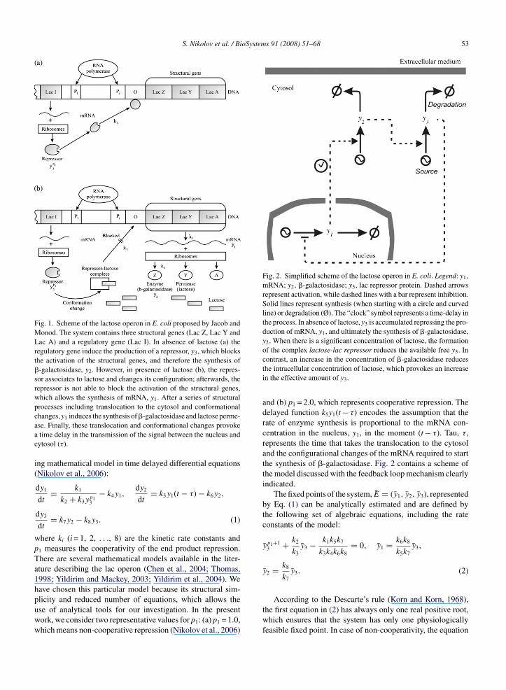

S. Nikolov et al. / BioSystems 91 (2008) 51–68 53

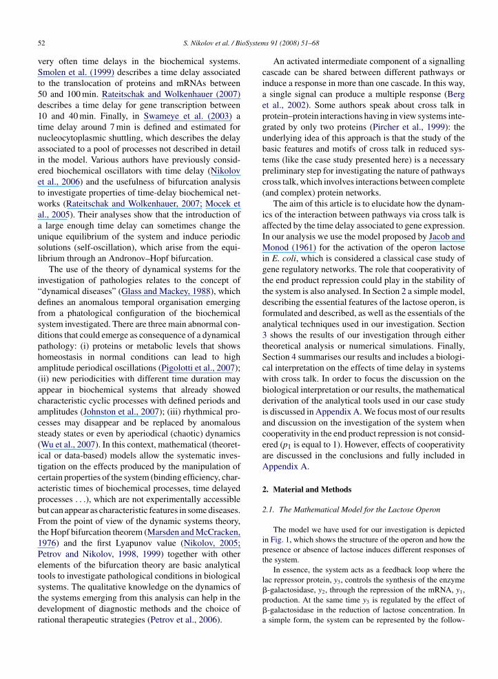
Fig. 1. Scheme of the lactose operon in E. coli proposed by Jacob andMonod. The system contains three structural genes (Lac Z, Lac Y andLac A) and a regulatory gene (Lac I). In absence of lactose (a) theregulatory gene induce the production of a repressor, y3, which blocksthe activation of the structural genes, and therefore the synthesis of�-galactosidase, y2. However, in presence of lactose (b), the repres-sor associates to lactose and changes its configuration; afterwards, therepressor is not able to block the activation of the structural genes,which allows the synthesis of mRNA, y1. After a series of structuralprocesses including translocation to the cytosol and conformationalcaac

i(

wpTa1hpuww

Fig. 2. Simplified scheme of the lactose operon in E. coli. Legend: y1,mRNA; y2, �-galactosidase; y3, lac repressor protein. Dashed arrowsrepresent activation, while dashed lines with a bar represent inhibition.Solid lines represent synthesis (when starting with a circle and curvedline) or degradation (Ø). The “clock” symbol represents a time-delay inthe process. In absence of lactose, y3 is accumulated repressing the pro-duction of mRNA, y1, and ultimately the synthesis of �-galactosidase,y2. When there is a significant concentration of lactose, the formationof the complex lactose-lac repressor reduces the available free y3. In

hanges, y1 induces the synthesis of �-galactosidase and lactose perme-se. Finally, these translocation and conformational changes provoketime delay in the transmission of the signal between the nucleus andytosol (τ).

ng mathematical model in time delayed differential equationsNikolov et al., 2006):

dy1

dt= k1

k2 + k3yp13

− k4y1,dy2

dt= k5y1(t − τ) − k6y2,

dy3

dt= k7y2 − k8y3. (1)

here ki (i = 1, 2, . . ., 8) are the kinetic rate constants and1 measures the cooperativity of the end product repression.here are several mathematical models available in the liter-ture describing the lac operon (Chen et al., 2004; Thomas,998; Yildirim and Mackey, 2003; Yildirim et al., 2004). We

ave chosen this particular model because its structural sim-licity and reduced number of equations, which allows these of analytical tools for our investigation. In the presentork, we consider two representative values for p1: (a) p1 = 1.0,hich means non-cooperative repression (Nikolov et al., 2006)

contrast, an increase in the concentration of �-galactosidase reducesthe intracellular concentration of lactose, which provokes an increasein the effective amount of y3.

and (b) p1 = 2.0, which represents cooperative repression. Thedelayed function k5y1(t − τ) encodes the assumption that therate of enzyme synthesis is proportional to the mRNA con-centration in the nucleus, y1, in the moment (t − τ). Tau, τ,represents the time that takes the translocation to the cytosoland the configurational changes of the mRNA required to startthe synthesis of �-galactosidase. Fig. 2 contains a scheme ofthe model discussed with the feedback loop mechanism clearlyindicated.

The fixed points of the system, E = (y1, y2, y3), representedby Eq. (1) can be analytically estimated and are defined bythe following set of algebraic equations, including the rateconstants of the model:

yp1+13 + k2

k3y3 − k1k5k7

k3k4k6k8= 0, y1 = k6k8

k5k7y3,

y2 = k8

k7y3. (2)

According to the Descarte’s rule (Korn and Korn, 1968),the first equation in (2) has always only one real positive root,which ensures that the system has only one physiologicallyfeasible fixed point. In case of non-cooperativity, the equation

oSystem

54 S. Nikolov et al. / Bi

describing the stationary values of y3 is simpler:

y3 = 1

2

⎛⎝−k2

k3+√(

k2

k3

)2

+ 4k1k5k7

k3k4k6k8

⎞⎠ (2.1)

2.2. Analytical Tools. Andronov–Hopf Bifurcation andFirst Lyapunov Value

The dynamical systems approach for the investigation ofpathologies considers that the analysis of non-linearity andbifurcations in mathematical for an understanding of the mech-anism of transition between the healthy and pathological states.Steady state and oscillatory solutions of the dynamical systembelong to the set of recurrent solutions. One of these solutionsis stable if any small perturbation disappears over time and thesystem returns to the vicinity of the initial state. If this returnis not accomplished (e.g., the amplitude of the perturbationincreases over time), the solution is unstable. Stable (steadystate and oscillatory) recurrent solutions represent physiolog-ically observable states in homeostatic and cyclic biologicalsystems. In addition, in self-sustained physiological oscilla-tions their characteristics are defined predominantly by internalproperties of the control system and not by external influences.

The nature of the recurrent solutions of a dynamical sys-tem depends on the values of the parameters. If a parametervalue is changed due to pathological (e.g., loss of functionalityin an enzyme due to structural deficiencies) or biotechnolog-ical motivations (e.g., changes in the rate of synthesis of acertain protein by artificial over expression), then the proper-ties of the recurrent solutions of the network may change. Forinstance, a steady state may lose its stability or even cease toexist, and a self-sustained oscillation may be into existence, abehaviour called the Andronov–Hopf bifurcation. This bifur-cation is well documented (Marsden and McCracken, 1976;Iooss and Joseph, 1990) and can be investigated by local anal-ysis, which is one of the analytical strategies used in this work.This bifurcation can be of two types: supercritical (soft lossof stability), which has been experimentally observed in manybiological systems (Petrov and Nikolov, 1998, 1999), and sub-critical (hard loss of stability). A subcritical Andronov–Hopfbifurcation leads to unstable solutions but may fold back andexhibit stable periodic solutions coexisting with stable steadystates. In general, qualitative changes in the nature of the recur-rent solutions when certain parameters are modified are calledbifurcations; these qualitative changes occur at specific valuesof the parameters called bifurcation points.

The Andronov–Hopf bifurcation is a rather widespreadmechanism in living organisms and there is a Hopf theorem thatpredicts the general conditions under which the correspondingbifurcation occurs and what the features of this bifurcation

are. In this way, using the Lyapunov function (Andronov et al.,1966; Bautin, 1984) or its corresponding index one can predictif stability in the solutions emerges from a bifurcation. But theuse of the First Lyapunov values (Nikolov, 2005; Petrov andNikolov, 1998, 1999 and Petrov et al., 2006), the other analyt-

s 91 (2008) 51–68

ical tool used in this work, has improved predictive abilitiesbecause it permits to decide whether the transition over thebifurcation point provokes either stability or instability. Thestability or instability of these transitions may have importantconsequences on the dynamics of the investigated system, lead-ing the system to pathological configurations and pointing outchanges in which parameters are critical for the emergence ofthe pathology.

3. Results

3.1. Theoretical Predictions

3.1.1. Andronov–Hopf Bifurcation AnalysisIn this section, we consider the system when the coop-

erativity in the end-product repression, p1, is equal to oneand all constants of the model are real positive numbers.We use Andronov–Hopf bifurcation analysis and con-sider the time delay τ as a bifurcation parameter. Let usconsider a small perturbation around the fixed point ofthe system E defined as:

y1 = y1 + x y2 = y2 + y y3 = y3 + z

If we expand the non-linear equation describing thefeedback loop, the equations describing the system aretransformed into:

dx

dt= −k4x − k1k3

δ2 z + k1k23

δ3 z2 − k1k33

δ4 z3,

dy

dt= k5�

−τχx − k6y,dz

dt= k7y − k8z (3)

where δ = k2 + k3y3. If we neglect terms of second andthird order, the stability matrix leads to the followingcharacteristic equation

χ3 + pχ2 + qχ + r1 = −A�−τχ (4)

where

p = k4 + k6 + k8, q = k4k6 + k4k8 + k6k8,

r1 = k4k6k8, A = k1k3k5k7

δ2 (5)

This characteristic Eq. (4) is transcendental and can-not be solved analytically. Moreover, it has an indefinitenumber of roots (Elsgolz and Norkin, 1974, and Khanand Greenhagh, 1999). In essence, we have two mainoptions besides a direct numerical investigation: (i) lin-ear stability analysis, which is valid only in case of small

time delays (see Appendix A for further details about thispossibility), and (ii) the Hopf bifurcation theorem (Cai,2005), which is the option we explore here. If we defineχ = m + in and rewrite (4) in terms of its real and imagi-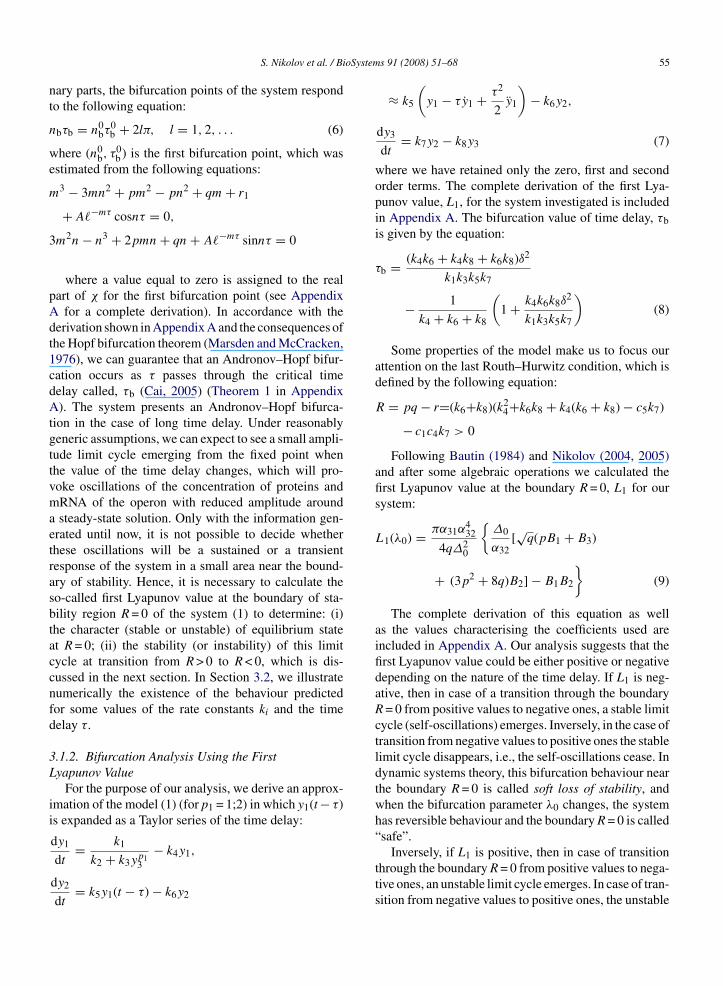

oSystem

nt

n

we

m

3

pAdt1cdAtgttvmaetrasbtaccnfd

3L

ii

Inversely, if L1 is positive, then in case of transitionthrough the boundary R = 0 from positive values to nega-

S. Nikolov et al. / Bi

ary parts, the bifurcation points of the system respondo the following equation:

bτb = n0bτ

0b + 2lπ, l = 1, 2, . . . (6)

here (n0b, τ

0b ) is the first bifurcation point, which was

stimated from the following equations:3 − 3mn2 + pm2 − pn2 + qm + r1

+ A�−mτ cosnτ = 0,

m2n − n3 + 2pmn + qn + A�−mτ sinnτ = 0

where a value equal to zero is assigned to the realart of χ for the first bifurcation point (see Appendix

for a complete derivation). In accordance with theerivation shown in Appendix A and the consequences ofhe Hopf bifurcation theorem (Marsden and McCracken,976), we can guarantee that an Andronov–Hopf bifur-ation occurs as τ passes through the critical timeelay called, τb (Cai, 2005) (Theorem 1 in Appendix). The system presents an Andronov–Hopf bifurca-

ion in the case of long time delay. Under reasonablyeneric assumptions, we can expect to see a small ampli-ude limit cycle emerging from the fixed point whenhe value of the time delay changes, which will pro-oke oscillations of the concentration of proteins andRNA of the operon with reduced amplitude aroundsteady-state solution. Only with the information gen-

rated until now, it is not possible to decide whetherhese oscillations will be a sustained or a transientesponse of the system in a small area near the bound-ry of stability. Hence, it is necessary to calculate theo-called first Lyapunov value at the boundary of sta-ility region R = 0 of the system (1) to determine: (i)he character (stable or unstable) of equilibrium statet R = 0; (ii) the stability (or instability) of this limitycle at transition from R > 0 to R < 0, which is dis-ussed in the next section. In Section 3.2, we illustrateumerically the existence of the behaviour predictedor some values of the rate constants ki and the timeelay τ.

.1.2. Bifurcation Analysis Using the Firstyapunov Value

For the purpose of our analysis, we derive an approx-mation of the model (1) (for p1 = 1;2) in which y1(t − τ)s expanded as a Taylor series of the time delay:

dy1

dt= k1

k2 + k3yp13

− k4y1,

dy2

dt= k5y1(t − τ) − k6y2

s 91 (2008) 51–68 55

≈ k5

(y1 − τy1 + τ2

2y1

)− k6y2,

dy3

dt= k7y2 − k8y3 (7)

where we have retained only the zero, first and secondorder terms. The complete derivation of the first Lya-punov value, L1, for the system investigated is includedin Appendix A. The bifurcation value of time delay, τbis given by the equation:

τb = (k4k6 + k4k8 + k6k8)δ2

k1k3k5k7

− 1

k4 + k6 + k8

(1 + k4k6k8δ

2

k1k3k5k7

)(8)

Some properties of the model make us to focus ourattention on the last Routh–Hurwitz condition, which isdefined by the following equation:

R = pq − r=(k6+k8)(k24+k6k8 + k4(k6 + k8) − c5k7)

− c1c4k7 > 0

Following Bautin (1984) and Nikolov (2004, 2005)and after some algebraic operations we calculated thefirst Lyapunov value at the boundary R = 0, L1 for oursystem:

L1(λ0) = πα31α432

4qΔ20

{Δ0

α32[√

q(pB1 + B3)

+ (3p2 + 8q)B2] − B1B2

}(9)

The complete derivation of this equation as wellas the values characterising the coefficients used areincluded in Appendix A. Our analysis suggests that thefirst Lyapunov value could be either positive or negativedepending on the nature of the time delay. If L1 is neg-ative, then in case of a transition through the boundaryR = 0 from positive values to negative ones, a stable limitcycle (self-oscillations) emerges. Inversely, in the case oftransition from negative values to positive ones the stablelimit cycle disappears, i.e., the self-oscillations cease. Indynamic systems theory, this bifurcation behaviour nearthe boundary R = 0 is called soft loss of stability, andwhen the bifurcation parameter λ0 changes, the systemhas reversible behaviour and the boundary R = 0 is called“safe”.

tive ones, an unstable limit cycle emerges. In case of tran-sition from negative values to positive ones, the unstable

oSystems 91 (2008) 51–68

56 S. Nikolov et al. / Bi

limit cycle disappears. This type of bifurcation behaviournear the boundary R = 0 is called hard loss of stability, thesystem has an irreversible behaviour, and the boundaryR = 0 is referred to as “dangerous” (Bautin, 1984).

As a consequence of our analysis, we can predict thata limit cycle will emerge if the time delay is higher thanτb, while the cycle limit will vanish if the time delayis smaller. In other words, as a result of the evidenceobtained through (A.27)–(A.30) (see Appendix A) and(8) we may conclude that in this case the time delay hasa destabilizing role because it changes drastically theproperties of the system when pass through the bifur-cation point provoking the emergence of a limit cycle.For time delays longer than the bifurcation value τb,the lactose operon would present sustained oscillationswith coupled periodic variations on the concentration ofboth proteins and the mRNA. In contrast, a time delaysmaller than τb will provoke only transient oscillationsof the species integrating the operon around a stablesteady state.

3.2. Numerical Analysis

In the previous two sections, we introduced the ana-lytical tools proposed and used them for a qualitativeanalysis of the system obtaining some predictions aboutthe dynamics of the system. In this section, we performa numerical analysis of the model based on the previ-ous results. The values chosen for the parameters andused in the numerical analysis were selected according to(Timmer et al., 2004; Fall et al., 2002; Jacob and Monod,1961 and Bliss et al., 1982) and are included in AppendixA. The analytical results stated in previous sections per-mit us to predict how the properties of the system vary

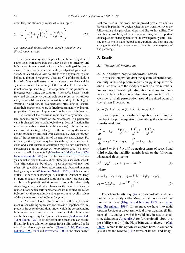
when the parameters in the model are modified. In Fig. 3we show the dependence on k3 and k5 of the criticalvalue of time delay in which the system goes through atransition to a stable limit cycle, τb.

Fig. 4. Stable (a) and unstable (b) solution of the

Fig. 3. Predicted values of τb (as function of k3 and k5) using analyticalformula (8) from Section 3.1.

The value of τb is quite sensitive to changes in bothparameters, especially k3. For example, a change of 50%in the value of k3 multiplies by three the value of thecritical time delay, and a change of 100% in k3 increasesthe value of the critical time delay up to 27 min. Thismeans that for very high values on k3, the transition tostable limit cycles will not appear in the system becauseit requires too long, biologically unfeasible, time delays(much longer than half an hour).

In order to compare the predictions with numericalresults, the governing equations of the model, repre-sented by (1), were solved numerically using MATLAB(Mathworks, 2007). The use of (8) permitted us tocompute a predicted value for the critic time delayof τb = 4.17 min when we fixed the parameters k1–k8(see (A.57) of Appendix A). In Fig. 4 we illustratethe dependence of the model behaviour on the value

for the time delay (around this predicted critic valueτb). Fig. 4a shows a simulation of the dynamics fory1, y2 and y3 when time delay is lower than the criticvalue τb(τ = 2.5). After several physiologically accept-

system (1) (p1 = 1) at τ = 2.5 and 6.5 min.

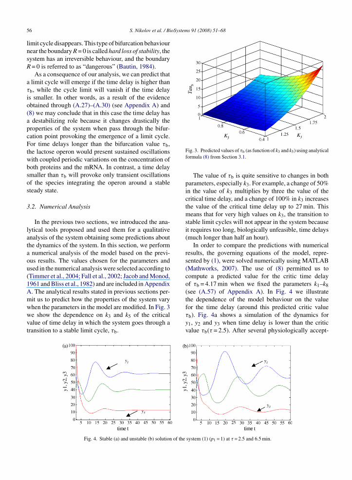
S. Nikolov et al. / BioSystems 91 (2008) 51–68 57

F he ampt

aeuwbpOcwti

Fk

ig. 5. Periodic solutions for mRNA (a) and repressor (b) at τ = 6.5. The values of both variables in the analysed state.

ble fluctuations, the variables describing mRNA, y1,nzyme, y2 and repressor, y3 approach to constant val-es that describe a steady state of the system. In otherords, in this case the Routh–Hurwitz condition for sta-ility is valid and the system (1) lies in a stable zone of itsarametric space. Notice that in this case R = 0.5168 > 0.n the other hand, Fig. 4b depicts the dynamics for the

ase of time delays higher than the critic value (τ = 6.5)here R is negative (R = −0.2397). Mathematically,

his state corresponds to a loss of stability. Accord-ng to the analytical results obtained in Section 3.1 we

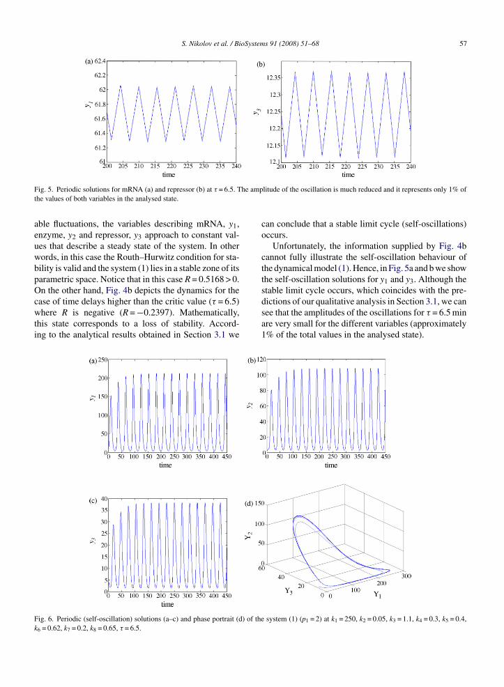
ig. 6. Periodic (self-oscillation) solutions (a–c) and phase portrait (d) of the

6 = 0.62, k7 = 0.2, k8 = 0.65, τ = 6.5.

litude of the oscillation is much reduced and it represents only 1% of

can conclude that a stable limit cycle (self-oscillations)occurs.

Unfortunately, the information supplied by Fig. 4bcannot fully illustrate the self-oscillation behaviour ofthe dynamical model (1). Hence, in Fig. 5a and b we showthe self-oscillation solutions for y1 and y3. Although thestable limit cycle occurs, which coincides with the pre-

dictions of our qualitative analysis in Section 3.1, we cansee that the amplitudes of the oscillations for τ = 6.5 minare very small for the different variables (approximately1% of the total values in the analysed state).

system (1) (p1 = 2) at k1 = 250, k2 = 0.05, k3 = 1.1, k4 = 0.3, k5 = 0.4,

oSystem

58 S. Nikolov et al. / Bi

These results shown in Fig. 5 need additional dis-cussion. The existence of cooperativity in protein-geneinteractions results in large changes in activation withsmall changes in protein concentration (Lehninger,2004). On the other hand, the minimum cooperativityrequired for oscillations becomes small when the lengthof the feedback loop increases. Since in the case anal-ysed we supposed low cooperativity and a short lengthfeedback loop, the limit cycle has small amplitude (Fallet al., 2002; Agnati et al., 2005). On the other hand, thecase when cooperativity is considered (p1 = 2) is shown

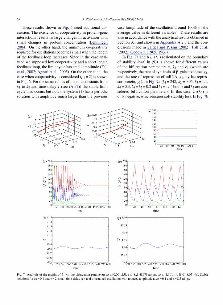
in Fig. 6. For the same values of the rate constants fromk1 to k8 and time delay τ (see (A.57)) the stable limitcycle also occurs but now the system (1) has a periodicsolution with amplitude much larger than the previous

Fig. 7. Analysis of the graphs of L1 vs. the bifurcation parameters k5 ∈ [0.0solutions for k5 = 0.1 and τ = 2, small time-delay (c), and a sustained oscillati

s 91 (2008) 51–68

case (amplitude of the oscillation around 100% of theaverage value in different variables). These results arealso in accordance with the analytical results obtained inSection 3.1 and shown in Appendix A.2.3 and the con-clusions made in Saltiel and Pessin (2002), Fall et al.(2002), Goodwin (1965, 1966).

In Fig. 7a and b L1(�0) (calculated on the boundaryof stability R = 0 in (9)) is shown for different valuesof the bifurcation parameters τ, k5 and k3 (which arerespectively, the rate of synthesis of �-galactosidase, y2,and the rate of repression of mRNA, y1, by lac repres-

sor protein, y3). In Fig. 7a (k1 = 248, k2 = 0.05, k3 = 1.1,k4 = 0.3, k6 = k7 = 0.2 and k8 = 1.1) both τ and k5 are con-sidered bifurcation parameters. In this case, L1(λ0) isonly negative, which ensures soft stability loss. In Fig. 7b

01,15], τ ∈ [8.,8.4897] (a) and k3 ∈ [1,10], τ ∈ [8.01,8.05] (b). Stableon with reduced amplitude at k5 = 0.1 and τ = 8.5 (d–g).

S. Nikolov et al. / BioSystems 91 (2008) 51–68 59

F ) whenk

(kes(cdH(

tsdFvttoir

4

qddbtfgos

tde

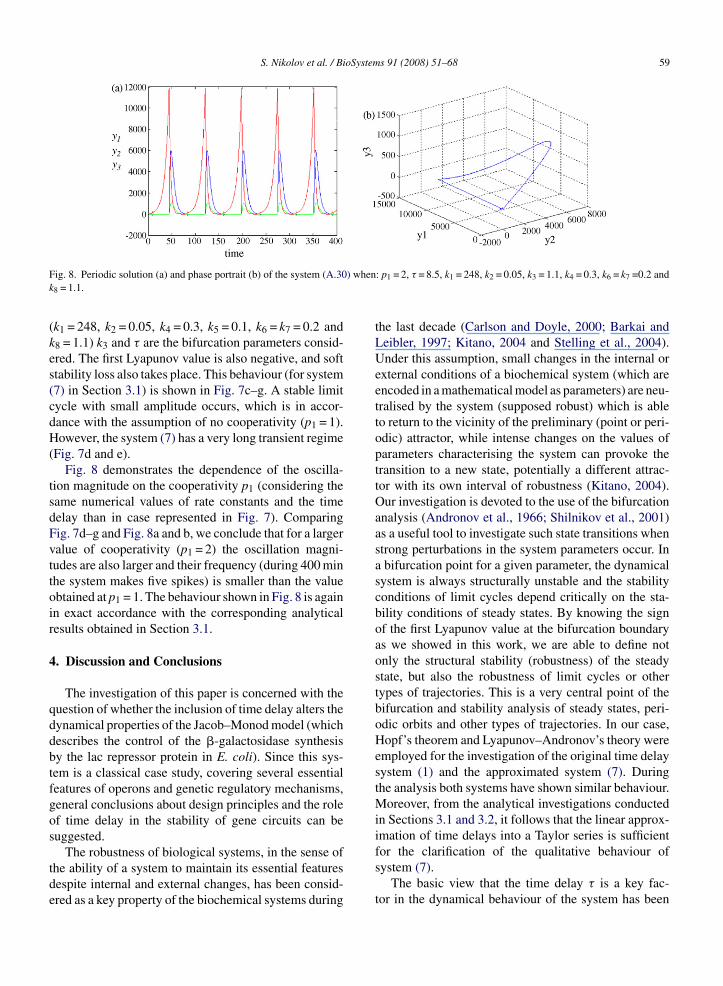
ig. 8. Periodic solution (a) and phase portrait (b) of the system (A.30

8 = 1.1.

k1 = 248, k2 = 0.05, k4 = 0.3, k5 = 0.1, k6 = k7 = 0.2 and8 = 1.1) k3 and τ are the bifurcation parameters consid-red. The first Lyapunov value is also negative, and softtability loss also takes place. This behaviour (for system7) in Section 3.1) is shown in Fig. 7c–g. A stable limitycle with small amplitude occurs, which is in accor-ance with the assumption of no cooperativity (p1 = 1).owever, the system (7) has a very long transient regime

Fig. 7d and e).Fig. 8 demonstrates the dependence of the oscilla-

ion magnitude on the cooperativity p1 (considering theame numerical values of rate constants and the timeelay than in case represented in Fig. 7). Comparingig. 7d–g and Fig. 8a and b, we conclude that for a largeralue of cooperativity (p1 = 2) the oscillation magni-udes are also larger and their frequency (during 400 minhe system makes five spikes) is smaller than the valuebtained at p1 = 1. The behaviour shown in Fig. 8 is againn exact accordance with the corresponding analyticalesults obtained in Section 3.1.

. Discussion and Conclusions

The investigation of this paper is concerned with theuestion of whether the inclusion of time delay alters theynamical properties of the Jacob–Monod model (whichescribes the control of the �-galactosidase synthesisy the lac repressor protein in E. coli). Since this sys-em is a classical case study, covering several essentialeatures of operons and genetic regulatory mechanisms,eneral conclusions about design principles and the rolef time delay in the stability of gene circuits can beuggested.

The robustness of biological systems, in the sense ofhe ability of a system to maintain its essential featuresespite internal and external changes, has been consid-red as a key property of the biochemical systems during

: p1 = 2, τ = 8.5, k1 = 248, k2 = 0.05, k3 = 1.1, k4 = 0.3, k6 = k7 =0.2 and

the last decade (Carlson and Doyle, 2000; Barkai andLeibler, 1997; Kitano, 2004 and Stelling et al., 2004).Under this assumption, small changes in the internal orexternal conditions of a biochemical system (which areencoded in a mathematical model as parameters) are neu-tralised by the system (supposed robust) which is ableto return to the vicinity of the preliminary (point or peri-odic) attractor, while intense changes on the values ofparameters characterising the system can provoke thetransition to a new state, potentially a different attrac-tor with its own interval of robustness (Kitano, 2004).Our investigation is devoted to the use of the bifurcationanalysis (Andronov et al., 1966; Shilnikov et al., 2001)as a useful tool to investigate such state transitions whenstrong perturbations in the system parameters occur. Ina bifurcation point for a given parameter, the dynamicalsystem is always structurally unstable and the stabilityconditions of limit cycles depend critically on the sta-bility conditions of steady states. By knowing the signof the first Lyapunov value at the bifurcation boundaryas we showed in this work, we are able to define notonly the structural stability (robustness) of the steadystate, but also the robustness of limit cycles or othertypes of trajectories. This is a very central point of thebifurcation and stability analysis of steady states, peri-odic orbits and other types of trajectories. In our case,Hopf’s theorem and Lyapunov–Andronov’s theory wereemployed for the investigation of the original time delaysystem (1) and the approximated system (7). Duringthe analysis both systems have shown similar behaviour.Moreover, from the analytical investigations conductedin Sections 3.1 and 3.2, it follows that the linear approx-imation of time delays into a Taylor series is sufficient

for the clarification of the qualitative behaviour ofsystem (7).

The basic view that the time delay τ is a key fac-tor in the dynamical behaviour of the system has been

oSystem

consider the time delay τ as a bifurcation parameter. Thefirst step is to obtain the characteristic equation for thelinearisation of the system near the equilibrium E. Let

60 S. Nikolov et al. / Bi

confirmed by the analytical calculations and numericalsimulations. From the qualitative theory of DDE andODE viewpoint, time delay appears as a bifurcationparameter on whose values depend the altered (stableor unstable) behaviour of the model. When no delayis considered in the synthesis of �-galactosidase (seeAppendix A), only a soft loss of stability take place,and changes of time delay through the critic value τbhas reversible behaviour. This means that at the tran-sition of R through the boundary R = 0 from positivevalues to negative ones a stable limit cycle emerges, i.e.,self-oscillations of the system appear. Inversely, at thetransition of R from negative values to positive ones thestable limit cycle disappears, i.e., the self-oscillationscease. However, when a time delay is considered theproperties of the system changes drastically, and hardloss of stability emerges. For time delays longer than τb,the lactose operon would present sustained oscillationswith coupled periodic variations on the concentration ofboth proteins and the mRNA. In contrast, a time delaysmaller than τb will provoke only transient oscillations ofthe species integrating the operon around a stable steadystate. We can say that in this situation time delay has adestabilizing role.

When simple (non-cooperative) inhibition of mRNAproduction by the lac repressor protein is considered(p1 = 1.0), oscillations in values of concentrations forproteins and mRNA appear but the amplitude of suchoscillations is much reduced (around 1% of the averageconcentration in the cases shown in Figs. 5 and 7). Ifthe system is not able to distinguish these fine-tuningoscillations, the lac operon would act as if an effectivequasi steady state exists. From a biological perspective,it could be reasonable to think that the system presentsat least local robustness with respect the concentrationof lactose (which is a primary carbon source of the sys-tem), and then this reduced amplitude oscillations wouldnot provoke a differentiated response of the system dur-ing the different phases of the oscillation. In contrast,when cooperativity in the repression of mRNA synthe-sis is considered (p1 = 2.0), the oscillations also occursbut the magnitude of this oscillations in the concentra-tion of proteins and mRNA is actually significant. Insome cases (Figs. 6 and 8) the cooperativity provokesoscillations with changes all-nothing for the concentra-tion of the proteins during the period of the oscillations.Therefore, the oscillations induced for time delays higherthan the critic value τ in a system with cooperativ-

bity could provoke clearly differentiated responses of thesystem during the period of the oscillations. The conclu-sion of our analysis is that in the case of the lac operonanalysed, not only time delay in galactosidase synthe-

s 91 (2008) 51–68

sis but also cooperativity in the end product repressionis necessary to induce a regime of effective sustainedoscillations.

From a physiological viewpoint, the hard (irre-versible) loss of stability might be related to theemergence of new configurations in the regulatorygene circuit that could lead the system into a patho-logic state. Similar behaviour has been already detectedand discussed in other biological systems with differ-ent nature such as cardiac pulsations and the ocularsystem (Petrov and Nikolov, 1998, 1999), but the con-clusion that we point out here for hard stability loss issuggested here by the first time for protein synthesissystems.

Future work includes an investigation into whethersystem (1) also has a chaotic (non-regular) behaviourfor some numerical values of the parameters and howthis relates to pathological configurations of the sys-tem (Alligood et al., 1996; Nikolov, 2005 and Wu etal., 2007). A prerequisite for such a research is theresult that the first Lyapunov value L1(λ0) (in (9)) canalso be positive, i.e., the stability boundary R = 0 isdangerous.

Acknowledgements

S. Nikolov wishes to thank Prof. Assen Dim-itrov for his valuable help and suggestions. Thiswork was supported by the European Commission 6thFramework program as part of the COSBICS projectunder contract LSHG-CT-2004-512060: www.sbi.uni-rostock.de/cosbics.

Appendix A

A.1. Andronov–Hopf Bifurcation Analysis.Derivation and Additional Cases Analysed

In this section, we consider the system when the coop-erativity in the end-product repression, p1, is equal to oneand all constants of the model are real positive numbers.Let E = (y1, y2, y3) denote the equilibrium point of thesystem. We use Andronov–Hopf bifurcation analysis and

us consider a small perturbation about the equilibriumlevel defined as

y1 = y1 + x y2 = y2 + y y3 = y3 + z (A.1)

oSystem

b

wtah

wsf

χ

w

p

r

tiKmedt

AS

lfil

χ

wro

S. Nikolov et al. / Bi

In the general case, the function k1/k2 + k3yp13 can

e written as a MacLaurin series:

k1

k2 + k3yp13

= k1

δ + k3η= k1

δ((k3/δ)η + 1)

= k1

δ

(1 − k3

δη +

(k3

δ

)2

η2

−(

k3

δ

)3

η3 + · · ·)

(A.2)

here δ = k2 + k3yp13 and η is a polynomial of z. If we

ake only linear, square and cubic terms from (A.2) andfter substitution of (A.1) into differential Eq. (1) weave

dx

dt= −k4x − k1k3

δ2 z + k1k23

δ3 z2 − k1k33

δ4 z3,

dy

dt= k5�

−τχx − k6y,dz

dt= k7y − k8z (A.3)

here δ = k2 + k3y3 when p1 = 1. If we neglect terms ofecond and third order, the stability matrix leads to theollowing characteristic equation

3 + pχ2 + qχ + r1 = −A�−τχ (A.4)

here

= k4 + k6 + k8, q = k4k6 + k4k8 + k6k8,

1 = k4k6k8, A = k1k3k5k7

δ2 (A.5)

This characteristic Eq. (A.4), which is a transcenden-al equation, cannot be solved analytically and has anndefinite number of roots (Elsgolz and Norkin, 1974;han and Greenhagh, 1999). In essence, we have twoain tools besides a direct numerical investigation: lin-

ar stability analysis, which is valid in case of small timeelays, and the Hopf bifurcation theorem (Cai, 2005). Inhe following section we analyse both cases.

.1.1. Effects of Small Time Delays Using Lineartability Analysis

For a small time delay (i.e., τ ≈ 1 min) the method ofinear stability analysis is a very convenient approach tond the bifurcation point of the system. In this case let

−χτ ≈ 1 − χτ; then the characteristic Eq. (A.4) becomes

3 + pχ2 + (q − Aτ)χ + r = 0 (A.6)

here r = r1 + A. By applying the Hopf bifurcation theo-em and the Routh–Hurwitz criteria, a Hopf bifurcationccurs at a value τ = τb where the following conditions

s 91 (2008) 51–68 61

are satisfied:

p>0, q − Aτb > 0, r > 0, R = p(q − Aτb) − r = 0

(A.7)

Let us define the function h, which represent the char-acteristic function in case of small time delays:

h(χ, τ) = χ3 + pχ2 + (q − Aτ)χ + r (A.8)

If we evaluate the roots of h at τ = τb, we obtain thefollowing values that represent the eigenvalues of thesystem in the approximation of small time delay:

χ1 = −p = −(k4 + k6 + k8) < 0,

χ2,3 = ±ik = ±i√

q − Aτb (A.9)

where i is the imaginary unit. In order to clarify theproperties of the system in the Andronov–Hopf bifurca-tion (τ = τb), we analyse the derivative of the eigenvaluesaround this value of time delay. If we differentiate implic-itly h(χ(τ), τ) we obtain:

dχ

dτ= − ∂h/∂τ

∂h/∂χ= − −Aχ

3χ2 + 2pχ + q − Aτ(A.10)

Then, we evaluate the required derivatives of h at τb.The two roots χ2 and χ3 are complex complementaryand therefore have identical real part. Thus, the resultfor χ2 is identical to the result for χ3. In the particularcase of χ2, we obtain

dχ2(τb)

dτ= ikA(−3k2 + q − Aτb − 2pki)

L2 + I2 (A.11)

where L = −3k2 + q − Aτb, I = 2pk. The real part of(A.11) has the form

Re

(dχ2(τb)

dτ

)= 2pk2A

L2 + I2 > 0 (A.12)

The inequality stated in (A.12) is sufficient to ensurethat the real part of the eigenvalue χ2(τ) at τ = τb has apositive slope. In this case, the use of the Hopf bifurcationtheorem predicts that the system will have a limit cyclefor a time delay with the critic value τ = τb when theapproximation for small time delays is used.

A.1.2. Effects of Large Time Delays Using HopfBifurcation Analysis

For larger time delays τ, the linear stability analysisof the previous section is no longer valid and we needto use an alternative approach. If we define χ = m + inand rewrite (A.4) in terms of its real and imaginary parts

oSystem

62 S. Nikolov et al. / Bi

we obtain∣∣∣∣∣∣∣m3 − 3mn2 + pm2 − pn2 + qm + r1

+ A�−mτ cosnτ = 0,

3m2n − n3 + 2pmn + qn + A�−mτ sinnτ = 0

(A.13)

In order to find the first bifurcation point, we set m = 0in the equations. Then, the above two equations reduceto the following∣∣∣∣∣−pn2 + r1 + A cosnτ = 0,

−n3 + qn + A sinnτ = 0(A.14)

These two equations in (A.14) can be solved numeri-cally, leading to (n0

b, τ0b ), the first bifurcation point. The

subsequent bifurcation points (nb, τb) satisfy the follow-ing relation:

nbτb = n0bτ

0b + 2lπ, l = 1, 2, . . . (A.15)

We can guarantee that (A.14) has at least one positiveroot, that is, there is at least one bifurcation point of thesystem. By squaring the two equations in (A.14), addingthem, and using properties of trigonometric functions, itfollows that

n6 + (p2 − 2q)n4 + (q2 − 2pr1)n2 + r21 − A2 = 0

(A.16)

Here, we note that this is a cubic equation in n2 thatdescribes the stability of the system. If the conditionr2

1 < A2 is satisfied, the left-hand side of the equationis positive for large values of n2 and negative for n = 0.This means that (A.16) has at least one positive real root.Moreover, according to (Khan, 2000), Lemma 1 (seeAppendix A) applies in this situation and provides uswith a series of necessary and sufficient conditions in thisequation to obtain at least one positive root. Moreover,when we introduce the variable z = n2

b, (A.16) reducesto

g(z)=z3+(p2−2q)z2+(q2 − 2pr1)z + r21 − A2 = 0

The derivative of this equation in z has the followingvalue:

g′(z) = 3z2 + 2(p2 − 2q)z + q2 − 2pr1

The interesting point is that g′(z)|τ=τb > 0 if nb isthe least positive simple root of Eq. (A.16). This prop-

erty will be used in the following demonstration. Let usdenote the characteristic equation without linear approx-imation

H(χ, τ) = χ3 + pχ2 + qχ + r1 + A�−τχ

s 91 (2008) 51–68

Again, in order to clarify the properties of the sys-tem in the studied fixed point (τ = τb), we analyse thederivative of the eigenvalues around this value of timedelay:

dχ

dτ= − ∂H/∂τ

∂H/∂χ= Aχ�−τχ

3χ2+2pχ + q − Aτ�−τχ(A.17)

If we evaluate the real part of this equation at the fixedpoint τ = τb and set χ = inb, we obtain

dm

dτ

∣∣∣∣τ=τb

= Re

(dχ

dτ

)∣∣∣∣τ=τb

= n2b[3n4

b + 2(p2 − 2q)n2b − 2pr1 + q2]

L21 + I2

1

where L1 = −3n2b + q − Aτb cosnbτb and I1 = 2pnb +

Aτb sin nbτb. The expression between brackets in theprevious equation coincides with g′(z) = 3z2 + 2(p2 −2q)z + q2 − 2pr1, and then we can guarantee thatg′(z)|τ=τb > 0. This means that this derivative ispositive:

dm

dτ

∣∣∣∣τ=τb

= Re

(dχ

dτ

)∣∣∣∣τ=τb

= n2bg

′(n2b)

L21 + I2

1

> 0 (A.18)

A.1.2.1. Derivation of Lemma 1 and Theorem 1.Lemma 1. Let us define

Δ = 1

27(4c3

2 − c21c

22 + 4c3

1c3 − 18c1c2c3 + 27c33)

and suppose that c3 > 0. Then necessary and sufficientconditions for the cubic equation

θ3 + c1θ2 + c2θ + c3 = 0

to have at least one single positive root for θ are (A) either(i) c1 < 0, c2 ≥ 0, c2

1 > 3c2, or (ii) c2 < 0; and (B) Δ < 0.

If we denote

H(χ, τ) = χ3 + pχ2 + qχ + r1 + A�−τχ

then

dχ

dτ= − ∂H/∂τ

∂H/∂χ= Aχ�−τχ

3χ2 + 2pχ + q − Aτ�−τχ(A.19)

Evaluating the real part of this equation at τ = τb andsetting χ = inb yield

dm

dτ

∣∣∣∣τ=τb

= Re

(dχ

dτ

)∣∣∣∣τ=τb

= n2b[3n4

b + 2(p2 − 2q)n2b − 2pr1 + q2]

L21 + I2

1

oSystem

wA

g

g

un

a(

Tauna

twfd

A

t

y

w

M

Q

h

x

wtsc

S. Nikolov et al. / Bi

here L1 = −3n2b + q − Aτb cosnbτb and I1 = 2pnb +

τb sin nbτb. Let z = n2b, then (A.16) reduces to

(z)=z3+(p2 − 2q)z2 + (q2 − 2pr1)z + r21 − A2 = 0.

Then for g′(z) we have

′(z) = 3z2 + 2(p2 − 2q)z + q2 − 2pr1

If nb is the least positive simple root of Eq. (A.16),nless this is a double root when we must take nb as theext root, thus g′(z) | > 0. Hence

dm

dτ

∣∣∣∣τ=τb

= Re

(dχ

dτ

)∣∣∣∣τ=τb

= n2bg

′(n2b)

L21 + I2

1

> 0. (A.20)

According to the Hopf bifurcation theorem (Marsdennd McCracken, 1976), the following statement is trueCai, 2005)

heorem 1. Assume that the conditions of Lemma 1re satisfied and nb is the least positive root of Eq. (A.13)nless this is a double root when we must take nb as theext root which is simple, then a Hopf bifurcation occurss τ passes through τb.

Hence, it is possible for a negative feedback loopo have an Andronov–Hopf bifurcation. In Section 3.2,e demonstrate numerically these types of behaviour

or some values of the rate constants ki and the timeelay τ.

.1.3. Investigation of the Case, When p1 = 2In this case, the equilibrium (steady state) value y3 of

he system (1) is

¯3 = M1 + M2 (A.21)

here M1 = 3√

(k1k5k7/2k3k4k6k8) + √Q,

2 = 3√

(k1k5k7/2k3k4k6k8) − √Q. Here

=(

k2

3k3

)3

+(

k1k5k7

2k3k4k6k8

)2

> 0. (A.22)

Following the same type of procedure, the system (1)as the form

˙ = −k4x − 2y3k1k3

δ2 z + k1k3(4k3y23 − δ)

δ3 z2

+4k1k23 y3

δ3 z3 + k1k23

δ3 z4,

y = k5�−τχ − k6y, z = k7y − k8z, (A.23)

here now (for p1 = 2) δ = k2 + k3y23. It is easy to see

hat structure of the system (A.23) like with this ofystem (A.3). Therefore, the analytical results for thease of no longer cooperativeness are valid for this case.

s 91 (2008) 51–68 63

Note that now A = 2k1k3k5k7y3/δ2. In other words, the

Andronov–Hopf bifurcation takes place.

A.2. Bifurcation Analysis Using First LyapunovValue. Derivation and Additional Cases Analysed

In this section we study the advantages of the useof the first Lyapunov value (Andronov et al., 1966;Bautin, 1984; Nikolov, 2004; Nikolov and Petrov, 2004;Shilnikov et al., 2001) for investigating in detail the qual-itative properties of the bifurcation behaviour for thesystem with respect to a time delay. For the purposes ofour analysis, we derive an approximation of the model(1) (for p1 = 1; 2) in which y1(t − τ) is expanded as aTaylor’s series of the time delay:

dy1

dt= k1

k2 + k3yp13

− k4y1,

dy2

dt= k5y1(t − τ) − k6y2

≈ k5

(y1 − τy1 + τ2

2y1

)− k6y2,

dy3

dt= k7y2 − k8y3 (A.24)

where we have retained only the first, second and thirdterms (i.e., up to quadratic one with respect to τ). Hence,the role of time delay in the qualitative behaviour of sys-tem (1) can be analysed. It is well known that replacingy1(t − τ) with higher order approximations of a Taylorseries is not better than applying lower order approxima-tion (Elsgoltz, 1957; Driver, 1977). The reason for thisparadoxical phenomenon consists in the circumstancethat the higher order terms in the second equation of(A.24) are, in principle, not small. For example, by apply-ing a ‘step by step’ method (Elsgoltz, 1957; Driver, 1977)to solve a time delay system in Taylor’s presentationwith higher order terms, a small parameter at the higherderivatives appears. On the contrary, in lower order termsapproximation a similar parameter does not appear. Thedetailed statement of this circumstance depends on theorder of system. In the present case, Taylor’s series canbe applied only up to quadratic approximation. Certainly,linear approximation is also admissible.

Following (Bautin, 1984; Nikolov, 2004; Nikolov,2005), we calculate the so-called first Lyapunov valueL (see Appendix A in (Nikolov and Petrov, 2004)

1or for a detailed discussion (Andronov et al., 1966;Shilnikov et al., 2001)) at the boundary of the stabil-ity region R = 0 of the system (A.24). In accordancewith the Lyapunov–Andronov theory we have: (i) the

oSystem

64 S. Nikolov et al. / Bi

sign of the Lyapunov’s value determines the character(stable or unstable) of the equilibrium state at R = 0; (ii)the character of the equilibrium state, at R = 0, qualita-tively determines the reconstruction of the phase portrait(including the stability or instability of the limit cycle)at the transition from R < 0 to R > 0 (Andronov et al.,1966; Bautin, 1984). When the system without cooper-ativity is considered, it is not difficult to obtain that theapproximate canonical form of (A.24),

dx

dt= −k4x − c1z + c2z

2 − c3z3,

dy

dt= c4x − k6y + c5z − c6z

2 + c7z3,

dz1

dt= k7y − k8z (A.25)

where

c1 = k1k3

δ2 , c2 = k1k23

δ3 , c3 = k1k33

δ4 ,

c4 = k5(1 + k4τ), c5 = k1k3k5τ

δ2 , c6 = k1k23k5τ

δ3 ,

c7 = k1k33k5τ

δ4 (A.26)

Hence, the Routh–Hurwitz conditions for stability ofthe steady state, defined by (2), are

p = k4 + k6 + k8 > 0, (A.27)

q = k4k6 + k4k8 + k6k8 − c5k7 > 0, (A.28)

r = k4k6k8 + c1c4k7 − c5k4k7 > 0, (A.29)

R = pq − r = (k6 + k8)(k24+k6k8+k4(k6+k8)−c5k7)

−c1c4k7 > 0 (A.30)

When conditions (A.29) or (A.30) are not valid, thesteady state (2.1) becomes unstable. This means thatthere are several different values for some of the rateconstants, ki(i = 1, 2, 3, . . ., 8), and time delay, τ, thatmake the coefficients R and r pass through bifurcationboundaries in the parametric space (p > 0, q > 0, r), (p > 0,q > 0, R) or (k1, k2, . . ., k8) where the steady state (2.1)could change its character (stable or unstable):

R = pq − r = 0, (A.31)

r = 0 (A.32)

Following (Bautin, 1984), we call L1 the first Lya-punov value at boundary R = 0 and l1 at the boundaryr = 0. Following (Bautin, 1984; Nikolov, 2005), after

s 91 (2008) 51–68

accomplishing some algebraic operations we calculatethe first Lyapunov value at the boundary R = 0 for thecase of a three-dimensional system. Thus, we obtain

L1(λ0) = πα31α432

4qΔ20

{Δ0

α32[√

q(pB1 + B3)

+ (3p2 + 8q)B2] − B1B2

}(A.33)

where

B1 = 2(α′31c2 − α′

32c6), B2 = α31c6 − α23c2,

B3 = 3(α23c3 − α13c7),

Δ0 = det

∣∣∣∣∣∣∣α11 α12 α13

α21 α22 α23

α31 α32 α33

∣∣∣∣∣∣∣ (A.34)

Here we note that

α11 = c1(k4 + k8), α21 = −[c1c4 + c5(k6 + k8)],

α31 = (k6 + k8)(k4 + k8), α12 = −k4(k6 + k8),

α22 = c4k8, α32 = c4k7, α13 = −(k6 + k8)√

q,

α23 = −c4√

q, α33 = 0 (A.35)

Consequently, (A.34) follows from

α′31 = α11α22 − α12α21, α′

32 = α11α32 − α12α31

(A.36)

From (A.33) it is easy to see that in this casethe first Lyapunov value can be positive or negative,i.e., hard and soft loss stability can take place. There-fore, time delay is a key factor in the bifurcationbehaviour of the model (A.24). In other words, inaccordance to the Lyapunov–Andronov theory for thegeneral case of a three-dimensional system, if the timedelay is higher or smaller than one bifurcation value τbwe have:

• If L1 is negative, then in case of transition throughthe boundary R = 0 from positive values to negativeones, a stable limit cycle (self-oscillations) emerges.Inversely, in the case of transition from negative val-ues to positive ones the stable limit cycle disappears,

i.e., the self-oscillations cease. In dynamic systemstheory, this bifurcation behaviour near the bound-ary R = 0 is called soft loss of stability, and whenthe bifurcation parameter λ0 changes, the system has

oSystem

•

arwiaojH(S

•

•

•

t

τ

A

pp

�y

c13 = −k1k3k5k7

δ4 (A.45)

The divergence of the flow (A.44) is

D3 = ∂x1 + ∂x2 + ∂x3 = S1 < 0. (A.46)

S. Nikolov et al. / Bi

reversible behaviour and the boundary R = 0 is called“safe”.If L1 is positive, then in case of transition through theboundary R = 0 from positive values to negative ones,an unstable limit cycle emerges. Inversely, in case oftransition from negative values to positive ones, theunstable limit cycle disappears. This type of bifur-cation behaviour near the boundary R = 0 is calledhard loss of stability, the system has an irreversiblebehaviour, and the boundary R = 0 is referred to as“dangerous” (Bautin, 1984).

In other words, in the case of safe boundaries, L1 < 0,slow drift of the parameters back into the stability

egion brings a system back into the original response,hereas in the dangerous case, L1 > 0, this is generally

mpossible. Obviously, safe and dangerous boundariesre distinguished mainly by the stability or instabilityf the corresponding equilibrium state, or periodic tra-ectory, on the boundary (Shilnikov et al., 1993, 2001).ere we could note that at the boundary of stability r = 0

positive feedback loop), two cases occur (Bautin, 1984;hilnikov et al., 2001; Nikolov and Bozhov, 2004):

If l1 is different to zero, then in case of a transitionfrom negative values to positive ones the equilibriumstate becomes unstable double point, the system hasirreversible behaviour and the boundary r = 0 is dan-gerous. Also, from the sign of the added condition

Δ∗ = −p2q2 + 4q3 (A.37)

We can have two cases: (i.1) if Δ* < 0, then the equilib-rium state becomes saddle-knot; (i.2) if Δ* > 0, thenthe equilibrium state becomes saddle-focus.If the first Lyapunov’s value l1 is zero, then the equi-librium state is stable.

In the terms of model (A.24), using (A.31), we obtainhe bifurcation value of time delay, τb

b = (k4k6 + k4k8 + k6k8)δ2

k1k3k5k7

− 1

k4 + k6 + k8

(1 + k4k6k8δ

2

k1k3k5k7

)(A.38)

.2.1. Investigation of the Case τ = 0, p1 = 1Before determining analytically L1, we must accom-

lish some transformations of the system (A.24) (τ = 0,1 = 1). First we express (A.24) in the form

3 = −(k4 + k6 + k8)y3 − k4k6k8y3 + k1k5k7

k2 + k3y3.

(A.39)

s 91 (2008) 51–68 65

Let us denote

w = y3 − y3. (A.40)

According to (A.2), the function 1/k2 + k3y3 inMaclaurin series has the form

1

k2 + k3y3= 1

δ + k3w= 1

δ((k3/δ)w + 1)

= 1

δ

(1 − k3

δw +

(k3

δ

)2

w2

−(

k3

δ

)3

w3 + . . .

), (A.41)

where δ = k2 + k3y3. Once again, if we take only linear,square and cubic terms from (A.41) and after substitutionof (A.40) into (A.39), Eq. (A.39) takes the form

�w = −(k4 + k6 + k8)w − (k4k6 + k4k8 + k6k8)w

−(

k4k6k8 + k1k3k5k7

δ2

)w + k1k

23k5k7

δ3 w2

− k1k33k5k7

δ4 w3 (A.42)

On the other hand, let

w = x1, w = x2, w = x3. (A.43)

After substitution of (A.43) into (A.42), the third-order ordinary differential Eq. (A.42) is reduced to threefirst-order differential equations:

x1 = S1x1 + S2x2 + S3x3 + S6x23 + c13x

33,

x2 = x1, x3 = x2 (A.44)

where the coefficients S1,S2,S3,S6 and c13 are denoted inNikolov (2004), and here have the form

S1 = −(k4 + k6 + k8), S2 = −(k4k6 + k4k8 + k6k8),

S3 = −(

k4k6k8 + k1k3k5k7

δ2

), S6 = k1k

23k5k7

δ3 ,

3

∂x1 ∂x2 ∂x3

Therefore, the system (A.44) is always dissipativeand has an attractor. Following (Bautin, 1984), the

oSystem

66 S. Nikolov et al. / Bi

Routh–Hurwitz conditions for stability of

y3 = 1

2

⎛⎝−k2

k3+√(

k2

k3

)2

+ 4k1k5k7

k3k4k6k8

⎞⎠ ,

y1 = k6k8

k5k7y3, y2 = k8

k7y3 (A.47)

can be written in the form

p = −S1 > 0, (A.48)

q = −S2 > 0, (A.49)

r = −S3 > 0, (A.50)

R = pq − r = S1S2 + S3 > 0. (A.51)

The notations p,q,r and R are taken from (Bautin,1984). Here, we note that the conditions (A.48)–(A.50)are always valid. When the condition (A.51) is not valid,the steady state (A.47) becomes unstable. In order todefine the type of stability loss of steady state (A.47)it is necessary to calculate the so-called first Lyapunovvalue ((Bautin, 1984; Nikolov and Petrov, 2004). In thecase of three first-order differential equations, this valuewas determined analytically in Nikolov (2004). Thus,now we obtain

L1(λ0) = 3πS22

4Δ20

(S22 + S1S3)c13 < 0 (A.52)

where λ0 is defined as value of S1,S2,S3 and c13for which the relation R = 0 takes place. According to(Nikolov, 2004), Δ0 = (S2

2 + S1S3)√

q. In other words,as a result of the evidence obtained in (A.52), we con-clude that when τ = 0, p1 = 1, L1 is always negative andfor the system (A.24) only a soft loss of stability takeplace, i.e., in this case the system (A.24) has reversiblebehaviour in the cases of transition through the boundaryR = 0 -negative feedback loop.

A.2.2. Investigation of the Case τ �= 0, p1 = 1.Square Approximation

Here, we investigate the role of τ in the qualita-tive behaviour of system (A.24) replacing y1(t − τ) withsquare order approximation of a Taylor’s series. Thus,the system (A.24) in local coordinates takes the form

x = −k4x − c1z + c2z2 − c3z

3,

y = c∗4x − k6y + c∗

5z + Ψ, z = k7y − k8z, (A.53)

s 91 (2008) 51–68

where

c∗4 = k5(1 + k4τ) + k2

4τ2

2,

c∗5 = k1k3k5

δ2

[τ + τ2

2

(k4 + 2k3

δ

)],

Ψ = −k1k23k5τ

2δ3

[2 + τ

(k4 + 3k3

δ

)]z2 + k1k

33k5τ

2δ4

×[

2 + τ

(k4 + 4k3

δ

)]z3 − 3k1k

53k5τ

2

2δ6 z4

+ k1k63k5

δ7 z5 − k1k3k5τ2

δ8 z6. (A.54)

It is seen that that the structure (from qualitativepoint of view) is one and the same with this of sys-tem (A.25). Therefore, we can conclude that the formof the first Lyapunov value is also the same and wehave not new behaviour types, i.e., when we take squareapproximation hard (irreversible) loss of stability andsoft (reversible) loss of stability take place, and the linearapproximation is sufficient.

A.2.3. Investigation of the Case τ �= 0, p1 = 2In this case the system (A.24) has one real positive

equilibrium point (A.21). Thus, the canonical form of(A.24) (using (A.1)) is:

x = −k4x − c∗∗1 z + c∗∗

2 z2 + c∗∗3 z3,

y = c∗∗4 x − k6y + c∗∗

5 z − c∗∗6 z2 − c∗∗

7 z3,

z = k7y − k8z, (A.55)

where

c∗∗1 = 2k1k3y3

δ2 , c∗∗2 = k1k3

(4k3y

23 − δ

)δ3 ,

c∗∗3 = 4k1k

23

δ3 , c∗∗4 = k5(1 + k4τ),

c∗∗5 = 2k1k3k5τy3

δ2 , c∗∗6 = k1k3k5τ(4y2

3k3 − δ)

δ3 ,

c∗∗7 = 4k1k

23k5τy3

δ3 (A.56)

Note that δ = k2 + k3y23 and we retain only the first,

second and third terms of z. It is seen that the structure

of the system (A.55) and (A.25) is very close. Thus,we obtain that for this case the analytical formula forL1 is concurring with those in (A.33), where now B3 =3(α13c7 − α23c3). Hence, we conclude that also soft andhard stability loss take place.

oSystem

At

pMFo

k

k

k

k

τ

wt

R

A

A

A

B

B

B

BB

C

C

C

C

D

E

E

E

F

S. Nikolov et al. / Bi

.3. Values for the Parameters of the Model Used inhe Numerical Analysis

The corresponding numerical values of the modelarameters ki and τ were extracted from Jacob andonod (1961); Bliss et al. (1982); Pircher et al. (1999);

all et al. (2002); Timmer et al. (2004) are the followingne:

1 = 250 [min−1], k2 = 0.05 [min−1],

3 = 1.1 [min−1], k4 = 0.3 [min−1],

5 = 0.4 [min−1], k6 = 0.62 [min−1],

7 = 0.2 [min−1], k8 = 0.65 [min−1],

∈ [2.5, 6.5]. (A.57)

Since the time delay is the bifurcation parameterhose properties we are studying, we allow to vary in

he interval referred.

eferences

gnati, L., Tarakanov, A., Guidolin, D., 2005. A simple mathemat-ical model of cooperativeness in receptor mosaics based on the“symmetry rule”. Biosystems 80 (2), 165–177.

lligood, K., Sauer, T., Yorke, J., 1996. Chaos. An Introduction toDynamical Systems. Springer.

ndronov, A., Witt, A., Chaikin, S., 1966. Theory of Oscillations.Addison-Wesley, Reading, MA.

arkai, N., Leibler, S., 1997. Robustness in simple biochemical net-works. Nature 387, 913–917.

autin, N., 1984. Behavior of Dynamical Systems Near the Boundaryof Stability, Nauka, Moscow (in Russian).

eltrami, E., 1987. Mathematics for Dynamic Modeling. AcademicPress, Inc., Boston.

erg, et al., 2002. Biochemistry, fifth ed. W.H. Freeman & Co. Ltd.liss, R., Painter, P., Marr, A., 1982. Role of feedback inhibition in

stabilizing the classical operon. J. Theor. Biol. 97, 177–193.ai, H., 2005. Hopf bifurcation in the IS-LM business cycle model

with time delay. Electron. J. Diff. Eq. 15, 1–6.arlson, J., Doyle, J., 2000. Highly optimized tolerance: robustness

and design in complex systems. Phys. Rev. Lett. 84, 2529–2532.hen, L., Aihara, K., 2002. A model of periodic oscillation for genetic

regulatory systems. IEEE Trans. Circuits Syst. 49 (10), 1429–1436.hen, L., Wang, R., Kobayashi, T., Aihara, K., 2004. Dynamics of

gene regulatory networks with cell division cycle. Phys. Rev. E 70,011909.

river, R., 1977. Ordinary and Delay Differential Equations. Springer-Verlag, New York.

lsgolz, L., Norkin, S., 1974. Introduction in time delay equations,Nauka, Moscow (in Russian).

lsgoltz, L., 1957. Differential Equations, Gosizdat, Moscow (in Rus-

sian).

ungdamrong, N., Iyengar, R., 2004. Modeling cell signaling net-works. Biol. Cell 96, 355–362.

all, C., Marland, E., Wagner, J., Tyson, J., 2002. Computational CellBiology. Springer.

s 91 (2008) 51–68 67

Galach, M., 2003. Dynamics of the tumor-immune systemcompetition—the effect of time delay. Int. J. Appl. Math. Comput.Sci. 13 (3), 395–406.

Glass, L., Mackey, M., 1988. From Clock to Chaos. The Rhythms ofLife. Princeton Univ. Press.

Goldbeter, A., 1995. A model for circadian oscillations in theDrosophila period protein (PER). Proc. R. Soc. Lond. B261 (1362),319–324.

Goodwin, B., 1965. Oscillatory behavior in enzymatic control pro-cesses. Adv. Enz. Regul. 3, 425–438.

Goodwin, B., 1966. An entrainment model for timed enzyme synthesisin bacteria. Nature 209, 479–481.

Iooss, G., Joseph, D., 1990. Elementary stability and bifurcation theory,second. ed. Springer.

Jacob, F., Monod, F., 1961. Genetic regulatory mechanisms in thesynthesis of proteins. J. Mol. Biol. 3, 318–356.

Johnston, M.D., Edwards, C.M., Bodmer, W.F., Maini, P.K., Chapman,S.J., 2007. Mathematical modeling of cell population dynamics inthe colonic crypt and in colorectal cancer. PNAS USA 104 (10),4008–4013.

Khan, Q., Greenhagh, D., 1999. Hopf bifurcation in epidemic modelswith a time delay in vaccination. IMA J. Math. Appl. Med. Biol.16, 113–142.

Khan, Q., 2000. Hopf bifurcation in multiparty political systems withtime delay in switching. Appl. Math. Lett. 13, 45–52.

Kitano, H., 2004. Biological Robustness. Nature 5, 826–837.Kolch, W., 2000. Meaningful relationship: the regulation of the

Ras/Raf/Mek/Erk pathway by protein interactions. Biochem. J.351, 289–305.

Korn, G., Korn, T., 1968. Mathematical Handbook for Scientists andEngineers. McGraw-Hill Book Company.

Lehninger, A., 2004. Principles of Biochemistry. Freeman ed., NewYork.

Marsden, J., McCracken, M., 1976. The Hopf Bifurcation and ItsApplications. Springer-Verlag, NY.

Matlab, 2007. The MathWorks, Inc. Natick, MA, USA www.mathworks.com.

Mocek, W., Rudnicki, R., Voit, E., 2005. Approximation of delays inbiochemical systems. Math. Biosci. 198, 190–216.

Nikolov, S., Bozhov, B., 2004. Bifurcations and chaotic behavior onthe Lanford system. Chaos Solitons Fract. 21, 803–808.

Nikolov, S., 2004. First Lyapunov value and bifurcation behavior ofspecific class of three-dimensional systems. Int. J. BifurcationChaos 14 (8), 2811–2823.

Nikolov, S., Petrov, V., 2004. New results about route to chaos inRossler system. Int. J. Bifurcation Chaos 14 (1), 293–308.

Nikolov, S., 2005. An alternative bifurcation analysis of theRose–Hindmarsh mode. Chaos Solitons Fract. 23, 1643–1649.

Nikolov, S., Kotev, V., Petrov, V., 2005. An alternative approach toinvestigating a time delay model of Jak-Stat signaling pathway.Compt. Rend. Acad. Bulg. Sci. 58 (6), 889–896.

Nikolov, S., Kotev, V., Georgiev, G., Petrov, V., 2006. Dynamical rolesof time delays in protein cross talk models. Compt. Rend. Acad.Bulg. Sci. 59 (3), 261–268.

Petrov, V., Nikolov, S., 1998. Valuation of the extraocular effectiveelastance on the base of dynamical model. Nonlinear Dyn. Psychol.Life Sci. 2 (1), 1–20.

Petrov, V., Nikolov, S., 1999. Rheodynamic model of cardiac pressurepulsations. Math. Biosci. 157 (1/2), 237–252.

Petrov, V., Nikolova, E., Wolkenhauer, O., 2005. Driver identificationof the RAS/RAF/MEK/ERK signal transduction pathway. Compt.Rend. Acad. Bulg. Sci. 58 (6), 639–644.

oSystem

tose operon: a mathematical modeling study and comparison withexperimental data. Biophys. J. 84, 2841–2851.

68 S. Nikolov et al. / Bi

Petrov, V., Peifer, M., Timmer, J., 2006. Bistability and self-oscillationsin cell cycle control. J. Bifurcation Chaos 16 (4), 1057–1067.

Pigolotti, S., Krishna, S., Jensen, M.H., 2007. Oscillation patterns innegative feedback loops. PNAS USA 104 (16), 6533–6537.

Pircher, T., Petersen, H., Gustafsson, J., Haldosen, L., 1999. ERKinteracts with STAT5a. Mol. Endocrinol. 13, 555–565.

Rateitschak, K., Wolkenhauer, O., 2007. Intracellular delay limitscyclic changes in gene expression. Math. Biosci. 205, 163–179.

Salazar, C., Hofer, T., 2006. Kinetic models of phosphorylation cycles:a systematic approach using the rapid-equilibrium approximationfor protein–protein interactions. Biosystems 83 (2), 195–206.

Saltiel, A., Pessin, J., 2002. Insulin signaling pathways in time andspace. Trends. Biochem. Sci. 12, 65–71.

Shilnikov, L., Shilnikov, A., Turaev, D., Chua, L., 2001. Methods ofQualitative Theory in Nonlinear Dynamics, Part II, World Scien-tific, Singapore.

Shilnikov, A., Shilnikov, L., Turaev, D., 1993. Normal forms andLorenz attractors. Int. J. Bifurcation Chaos 1 (4), 1123–1139.

Smolen, P., Baxter, D., Byrne, J., 1998. Frequency selectivity, multista-bility, and oscillations emergy from models of genetic regulatorysystems. Am. J. Physiol. 274 (2), 532–542.

Smolen, P., Baxter, D.A., Byrne, J.H., 1999. Effects of macromolec-ular transport and stochastic fluctuations on dynamics of genetic

regulatory systems. Am. J. Physiol. 277 (4 Pt 1), C777–C790.

Swameye, I., Mueller, T.G., Timmer, J., Sandra, O., Klingmueller,U., 2003. Identification of nucleocytoplasmic cycling as a remotesensor in cellular signaling by data-based modelling. PNAS 100,1028–1033.

s 91 (2008) 51–68

Stelling, J., Sauer, U., Szallasi, Z., Doyle, F.I., Doyle, J., 2004. Robust-ness of cellular functions. Cell 118, 675–685.

Thomas, R., 1998. Laws for the dynamics of regulatory networks. Int.J. Dev. Biol. 42, 479–485.

Timmer, J., Muller, T., Swameye, I., Sandra, O., Klingmuller, U., 2004.Modeling the nonlinear dynamics of cellular signal transduction.Int. J. Bifurcation Chaos 14, 2069–2079.

Vera, J., Balsa-Canto, E., Wellstead, P., Banga, J.R., Wolkenhauer, O.,2007a. Power-Law Models of signal transduction pathways. Cell.Signal. 19, 1531–1541.

Vera, J., Curto, R., Cascante, M., Torres, N.V., 2007b. Detection ofpotential enzyme targets by metabolic modelling and optimisa-tion. Application to a simple enzymopathy. Bioinformatics 23,2281–2289.

Wolf, D., Eeckman, E., 1998. On the relationship between genomicregulatory element organization and gene regulatory dynamics. J.Theor. Biol. 195 (2), 167–186.

Wu, X., Lu, J., Wong, S., 2007. Suppression and generation of chaosfor a three-dimensional autonomous system using parametric per-turbation. Chaos Solitons Fract. 31 (4), 811–819.

Yildirim, N., Mackey, M., 2003. Feedback regulation in the Lac-

Yildirim, N., Santillan, M., Horike, D., Mackey, M., 2004. Dynamicsand bistability in a reduced model of lac operon. Chaos 14 (2),279–292.