DYNAMIC MODELING ISSUES

FOR POWER SYSTEM APPLICATIONS

A Thesis

by

XUEFENG SONG

Submitted to the Office of Graduate Studies of Texas A&M University

in partial fulfillment of the requirements for the degree of

MASTER OF SCIENCE

December 2003

Major Subject: Electrical Engineering

brought to you by COREView metadata, citation and similar papers at core.ac.uk

provided by Texas A&M University

DYNAMIC MODELING ISSUES

FOR POWER SYSTEM APPLICATIONS

A Thesis

by

XUEFENG SONG

Submitted to Texas A&M University

in partial fulfillment of the requirements for the degree of

MASTER OF SCIENCE

Approved as to style and content by:

____________________________ Garng M. Huang (Chair of Committee)

_____________________________ ____________________________ Ali Abur Henry F. Taylor (Member) (Member)

_____________________________ ____________________________ Du Li Chanan Singh (Member) (Head of Department)

December 2003

Major Subject: Electrical Engineering

iii

ABSTRACT

Dynamic Modeling Issues

for Power System Applications. (December 2003)

Xuefeng Song, B.S., Shandong University;

M.E., Dalian Maritime University

Chair of Advisory Committee: Dr. Garng M. Huang

Power system dynamics are commonly modeled by parameter dependent

nonlinear differential-algebraic equations (DAE) ),,( pyxfx =& and ),,(0 pyxg= . Due to

the algebraic constraints, we cannot directly perform integration based on the DAE.

Traditionally, we use implicit function theorem to solve for fast variables y to get a

reduced model in terms of slow dynamics locally around x or we compute y numerically

at each x. However, it is well known that solving nonlinear algebraic equations

analytically is quite difficult and numerical solution methods also face many

uncertainties since nonlinear algebraic equations may have many solutions, especially

around bifurcation points. In this thesis, we apply the singular perturbation method to

model power system dynamics in a singularly perturbed ODE (ordinary-differential

equation) form, which makes it easier to observe time responses and trace bifurcations

without reduction process. The requirements of introducing the fast dynamics are

investigated and the complexities in the procedures are explored. Finally, we propose

PTE (Perturb and Taylor’s expansion) technique to carry out our goal to convert a DAE

to an explicit state space form of ODE. A simplified unreduced Jacobian matrix is also

iv

introduced. A dynamic voltage stability case shows that the proposed method works well

without complicating the applications.

v

To my family

vi

ACKNOWLEDGMENTS

I would like to thank my advisor, Dr. Garng M. Huang, for his continuous

guidance, support and encouragement throughout my thesis work. I am thankful to my

committee members Dr. Ali Abur, Dr. Henry F. Taylor, and Dr. Du Li for their help and

time.

vii

TABLE OF CONTENTS

Page

ABSTRACT…………………………………….………………………………….…. iii

DEDICATION……………………………………………………………………....... v

ACKNOWLEDGMENTS…………………………………………………………….. vi

TABLE OF CONTENTS……………………………………………………………... vii

LIST OF FIGURES………………………………………………………………….... ix

LIST OF TABLES……………………………………………………………………. xii

CHAPTER

I INTRODUCTION…………………………………………………………... 1

1.1 Overview of Dynamic Modeling Issues of Power Systems……….. 1 1.2 Objectives and Organization of This Thesis………………………. 4

II ISSUES OF DIFFERENTIAL-ALGEBRAIC EQUATION (DAE) MODELING………………...………………………………………………. 7

2.1 Parameter Dependent DAE System……………......……………... 7 2.2 Bifurcation Analysis……………………………..……………….. 9 2.3 Fundamental Insights of the Modeling Approaches…………........ 22 2.4 The Requirements of Using the Singularly Perturbed ODE........... 53 2.5 Complexities of Building Fast Dynamics.…………………..….... 58 2.6 Summary………………………………………….…………….... 61

III THE TECHNIQUE OF PTE: PERTURB AND TAYLOR’S EXPANSION………………………………………………………..…....... 63

3.1 Describe Fast Dynamics by PTE…………………..………..….... 63 3.2 Case Study…………………………………..………………......... 67 3.3 Summary.…………………………………….………………….... 84

viii

CHAPTER Page

IV CONCLUSIONS………………………………………………….……...... 86

REFERENCES……………………………………………………………………...... 89

VITA………………………………………………………………………………..... 92

ix

LIST OF FIGURES

FIGURE Page

1 An illustration of a bifurcation point…………………………………………. 12

2 Saddle-Node………………………………………………………………….. 13

3 Purely imaginary eigenvalues (λ=±jω) occur at Hopf bifurcation………….... 14

4 The instability mechanism of Hopf bifurcations…………………………....... 16

5 C: singularity-induced bifurcation, B: saddle-node bifurcation…………….... 19

6 Singularity-induced bifurcation as p=0.125………………………………….. 21

7 The curves of f1(x, p) for different values of p……………………………….. 27

8 The curves of f2(x, p) for different values of p……………………………….. 27

9 The p-y curve of the DAE system……………………………………………. 30 10 Two components C+ and C_ divided by IS………………………………….. 32

11 Saddle-node B……………………………………………………………….. 35

12 Stability boundary in X space for p=0.14 in C+……………………………..... 37

13 Time response of (2.44a) converges to xM=xe1=0.3818...…………….…….... 37

14 Stability boundary in C_ in X space for p=0.08……………………………... 38

15 Stability boundary in C+ in X space for p=0.08.…………………………........ 38

16 Time response of (2.44b) converges to xL=xe2=0.8………………..……......... 39

17 Time response of (2.44a) converges to xH=0.1789……………….………….. 40

18 The singularly perturbed ODE defined in components C+ and C_………….. 43

x

FIGURE Page

19 The p-y curve of the ODE system...………………………………………….. 46

20 Phase portrait as p=0.08……………………………………………………… 47

21 Stability boundary of the stable equilibrium point H in C+ in X space as p=0.08…………………………………………………… 48

22 Stability boundary of the stable equilibrium point L in C_ in X space as p=0.08…………………………………………………… 48

23 Time response converges to H: (xH, yH)=(0.8944, 0.1789)…………………... 49

24 Time response converges to L: (xL, yL)=(0.8, 0.2)…………………………… 49

25 Phase portrait as p=0.125…………………………………………………….. 50

26 Phase portrait as p=0.14……………………………………………………… 51

27 Phase portrait as p≥0.1545…………………………………………………… 52

28 A two-bus power system…………………………………………………….. 68

29 The P-V curve…………………………………………………………….….. 72

30 Time response of E’ converges to the stable equilibrium E’=1.0199……….. 75 31 Time response of Efd converges to the stable equilibrium Efd=1.983..………. 75

32 Time response of E converges to the stable equilibrium E=0.79…....………. 76

33 Time responses of E’, Efd, and E diverge away from the unstable equilibrium E’=0.996, Efd = 2.018, E=0.72………………..…………............ 76

34 Time responses of E’, Efd, and E monotonically diverge.…………………… 78

35 The eigenvalues approach to infinity at SIB point C………………………… 80

36 Time response of E’ initial at E’(0)=1.048..…………………………………. 80

37 Time response of Efd initial at Efd(0)=1.9…...……………………………….. 81

38 Time response of E initial at E(0)=0.834…………………………………….. 81

xi

FIGURE Page

39 Break-away point D and break-in point C…………………………………… 83

xii

LIST OF TABLES

TABLES Page

I Equilibrium points and eigenvalues of the DAE system……………….......... 29

II Equilibrium points and eigenvalues of the ODE system compared with the original DAE system…..………………………………… 45

III Eigenvalues of the three systems…………………………………………….. 59

IV Sign adjustment for m=2……………………………………………………... 60

V Hopf bifurcation point A…………………………………………………….. 74

VI Saddle-node bifurcation point B…………………………………………….. 77

VII Singularity-induced bifurcation point C…………………………………….. 79

VIII A break-away point D introduced by TJM and Point C becomes a break-in point………………………………………. 84

1

CHAPTER I

INTRODUCTION

In the last two decades, power systems have been operated under much more

stressed conditions than in the past. This is largely due to the environmental pressures on

transmission expansion, increased electricity consumption in heavy load areas, new

system loading patterns for the deregulated electricity market, etc. Under these stressed

conditions, a power system can exhibit a new type of dynamic unstable behaviors such as

slow voltage drops, or even voltage collapse [1], [2], [3]. Therefore, the need for power

system dynamic analysis has grown significantly in recent years.

The objective of this thesis is studying the dynamic modeling issues of power

systems. We will propose improved and approximated modeling approaches, as well as

power system examples to demonstrate the approaches and their applications.

1.1 Overview of Dynamic Modeling Issues of Power Systems

Power system dynamics are commonly expressed in a differential-algebraic

equation (DAE) form [1], [4]

kmn

mqmn

nqmn

PpYyXx

gpyxgfpyxfx

ℜ⊂∈ℜ⊂∈ℜ⊂∈

⎪⎩

⎪⎨⎧

ℜ→ℜ=

ℜ→ℜ=++

++

,,

)2.1(:),,,(0)1.1(:),,,(&

_______________________

This thesis follows the style of the IEEE Transactions on Automatic Control.

2

where the parameter p defines specific system configurations and operation conditions,

such as loads, generation, voltage setting points, etc. The dynamic state x (slow modes)

describes the generation dynamics of power systems, such as exciter control systems.

The instantaneous variables y (fast modes) satisfies algebraic constraints (1.2), such as

power flow equations, which is implicitly assumed to have an instantaneously

converging transient.

We analyze power system dynamics through observing time responses and

eigenvalue solutions [3]. However, it is difficult to analyze and simulate the nonlinear

DAE due to the instantaneous dynamic nature of algebraic constraints, which is only

true in the approximation sense. Traditionally, we use implicit function theorem to solve

for fast variables y to get a reduced model in terms of slow dynamics locally around x.

Or we compute y numerically at each x. The reduced Jacobian matrix of DAE is often

used in the analysis of power system dynamics [3], [5]. The linearized dynamic

expression of DAE is as below [1], [6]:

⎥⎦

⎤⎢⎣

⎡∆∆

=⎥⎦

⎤⎢⎣

⎡∆yx

Jx

u0&

(1.3)

⎥⎦

⎤⎢⎣

⎡=

yx

yxu gg

ffJ (1.4)

DAE (1.3) can be reduced to an ODE (ordinary-differential equation) when gy is

nonsingular, i.e., the algebraic variable y∆ can be eliminated from (1.3) [1]

)5.1(][ 1 xJxggffx rxyyx ∆=∆−=∆ −&

)6.1(][ 1xyyxr ggffJ −−=

3

where Jr is called the reduced Jacobian matrix (RJM) as opposed to the unreduced

Jacobian matrix (UJM) Ju. The stability of an equilibrium point of the DAE system for a

given p depends on the eigenvalues of the reduced Jacobian matrix Jr [1]. Through

tracing the eigenvalues of matrix Jr, we can study the local dynamic stability of the

systems [1], [7]. There are two steps involved to identify the dynamic stability of power

systems as the parameter p slowly changes. First, solve and trace the equilibrium point

along the path, which is defined by a scheduled system operating strategy. Then, form

RJM and analyze the eigenvalues at each equilibrium point [1], [8], [9].

The reduction computation may not be trivial. It is well known that solving

nonlinear algebraic equations analytically is quite difficult. Numerical methods can be

used to solve DAE systems. The procedure involves alternately solving the algebraic

power flow equations representing the network and the differential equations

representing the machines [6], [10]. We may use Gauss-Seidel (or Newton-Raphson)

method to solve nonlinear algebraic equations (power flow equations) and Euler’s

method (or Runge-Kutta method) to get the solutions of differential equations [10]. The

integration and algebraic solving are alternately applied and the procedure is messy. For

large power systems, if the initial condition is far from a solution point of the power flow

or the power flow problem is an ill-conditioned one, convergence of the power flow

solutions can be significantly slow or does not exist at all [11]. In addition, algebraic

constraints are approximations of fast dynamics, which assumes that the fast variable

converges to its equilibrium state instantaneously. Even if this is almost true, the

4

approximation may make its dynamic response too fast to be observed and the

interaction between fast modes and slow modes may become unclear.

Compared to RJM, the unreduced Jacobian matrix (UJM) Ju in (1.4) is simpler

and attractive to use in power system applications. Unfortunately, using this Ju may not

be able to obtain the exact system dynamic behaviors due to the unknown fast

dynamics y& . The singular perturbation provides a way to deal with this issue [8], [12].

Paper [8] uses sign adjustment to model power system dynamics where a UJM is used in

bifurcation analysis. However it is difficult for cases with high dimensional power flow

constraints. In addition, decision on sign change is a big computation burden itself. Paper

[12] derives an approximated expression of fast dynamics but does not analyze the

dynamics based on the approximation in details. When it is used in the dynamic voltage

stability studies, we find that the singularity-induced bifurcation (SIB) of the original

DAE system is not preserved. The eigenvalue loci near the singular point are quite

different from those of the original DAE system. All these make the approximation

questionable.

1.2 Objectives and Organization of This Thesis

In this thesis, we introduce our new approach to model power system dynamics

in a singularly perturbed ODE, which can be directly integrated to obtain time responses

to avoid solving the nonlinear algebraic equations. The bifurcation properties of the

original DAE system are preserved by the ODE.

The idea of our new modeling approach is based on the following considerations:

5

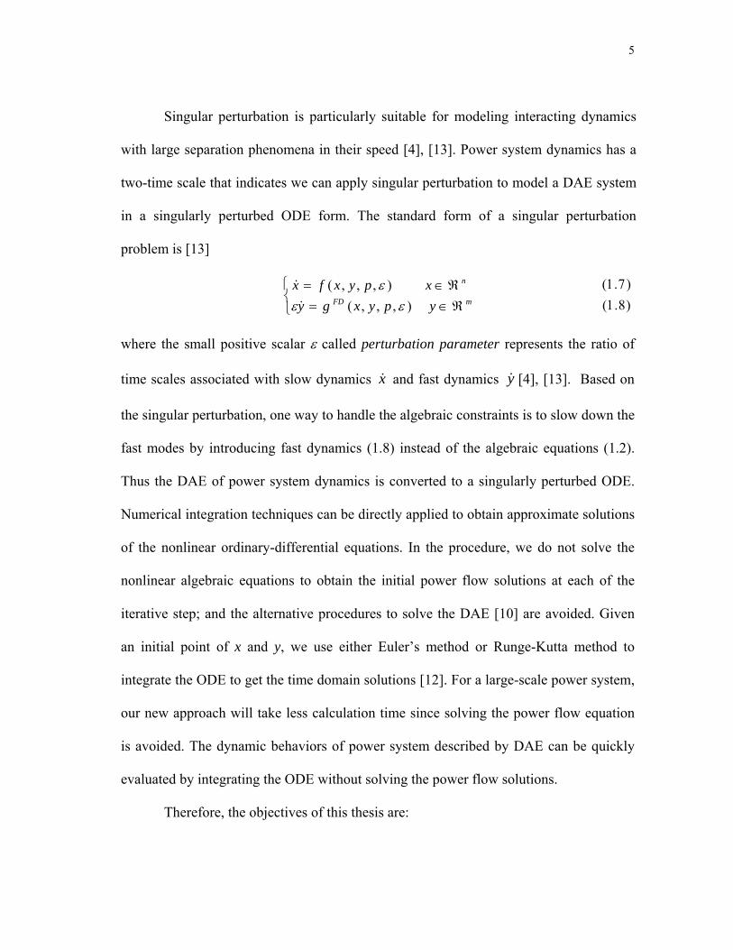
Singular perturbation is particularly suitable for modeling interacting dynamics

with large separation phenomena in their speed [4], [13]. Power system dynamics has a

two-time scale that indicates we can apply singular perturbation to model a DAE system

in a singularly perturbed ODE form. The standard form of a singular perturbation

problem is [13]

)8.1()7.1(

),,,(),,,(

⎩⎨⎧

ℜ∈=ℜ∈=

mFD

n

ypyxgyxpyxfx

εεε

&

&

where the small positive scalar ε called perturbation parameter represents the ratio of

time scales associated with slow dynamics x& and fast dynamics y& [4], [13]. Based on

the singular perturbation, one way to handle the algebraic constraints is to slow down the

fast modes by introducing fast dynamics (1.8) instead of the algebraic equations (1.2).

Thus the DAE of power system dynamics is converted to a singularly perturbed ODE.

Numerical integration techniques can be directly applied to obtain approximate solutions

of the nonlinear ordinary-differential equations. In the procedure, we do not solve the

nonlinear algebraic equations to obtain the initial power flow solutions at each of the

iterative step; and the alternative procedures to solve the DAE [10] are avoided. Given

an initial point of x and y, we use either Euler’s method or Runge-Kutta method to

integrate the ODE to get the time domain solutions [12]. For a large-scale power system,

our new approach will take less calculation time since solving the power flow equation

is avoided. The dynamic behaviors of power system described by DAE can be quickly

evaluated by integrating the ODE without solving the power flow solutions.

Therefore, the objectives of this thesis are:

6

• Remodel the DAE by a singularly perturbed ODE to avoid solving the

nonlinear algebraic equations so that we can directly integrate the ODE without

reduction process.

• Investigate the requirements and explore the complexities to introduce the fast

dynamics.

• Propose PTE (Perturb and Taylor’s Expansion) technique to build the fast

dynamics. Thus, by PTE, a DAE is converted to a singularly perturbed ODE.

The organization of the thesis is as below:

• In chapter II, we present fundamental insights of our modeling approach. A

detailed dynamic analysis of a DAE system is demonstrated and compared

with the singularly perturbed ODE form. We then investigate the requirements

and explore the complexities of applying our new modeling approach. Some

associated mathematical background materials on bifurcation analysis are

provided.

• In chapter III, we present the technique of PTE (Perturb and Taylor’s

Expansion) to derive a generic expression of fast dynamics. A simplified

unreduced Jacobian matrix is also proposed which can be used in the

eigenvalue analysis. A power system example is given to demonstrate our

proposals.

• Finally, all conclusions will be presented in chapter IV.

7

CHAPTER II

ISSUES OF DIFFERENTIAL-ALGEBRAIC EQUATION (DAE)

MODELING

In this chapter, we present fundamental insights of our modeling approach. A

detailed dynamic analysis of a DAE system is demonstrated and compared with our

singularly perturbed ODE. We then discuss the requirements and the complexities to

describe fast dynamics. A quick review of needed mathematical background is also

provided. We focus on DAE systems, bifurcation analysis, and our singular perturbation

approach.

2.1 Parameter Dependent DAE System

Parameter dependent DAE of the form

kmn

mkmn

nkmn

PpYyXx

gpyxgfpyxfx

ℜ⊂∈ℜ⊂∈ℜ⊂∈

⎪⎩

⎪⎨⎧

ℜ→ℜ=

ℜ→ℜ=++

++

,,

)2.2()1.2(

:),,,(0:),,,(&

is widely used to model the dynamics of physical systems, such as dynamic voltage

stability of power systems [1], [12], [14]. In the parameter-state space of X, Y, P, x is a

vector of n state variables, y is a vector of m algebraic variables, and p is a vector of k

parameter variables, which are changing slowly. The m algebraic equations (2.2) define

an n+k dimension manifold, called constraint manifold, in the n+m+k dimensional

parameter-state space of X, Y, P. System equilibrium points (xe, ye) satisfying

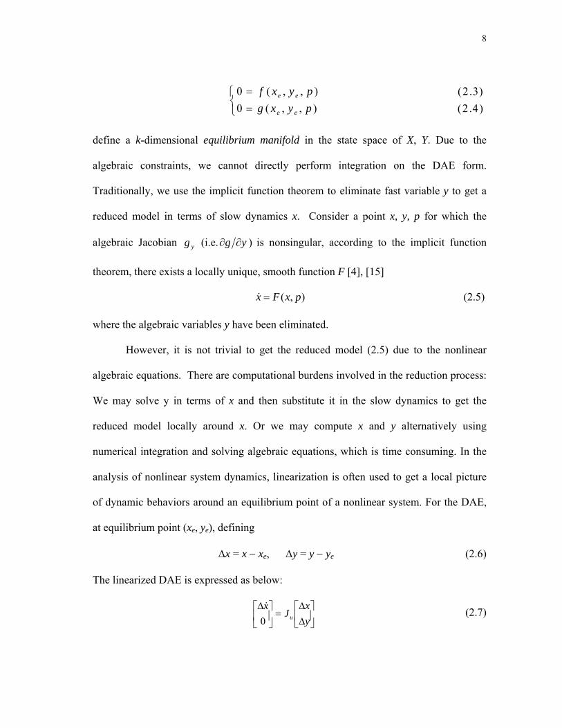
8

)4.2()3.2(

),,(0),,(0

⎩⎨⎧

==

pyxgpyxf

ee

ee

define a k-dimensional equilibrium manifold in the state space of X, Y. Due to the

algebraic constraints, we cannot directly perform integration on the DAE form.

Traditionally, we use the implicit function theorem to eliminate fast variable y to get a

reduced model in terms of slow dynamics x. Consider a point x, y, p for which the

algebraic Jacobian yg (i.e. yg ∂∂ ) is nonsingular, according to the implicit function

theorem, there exists a locally unique, smooth function F [4], [15]

(2.5)),( pxFx =&

where the algebraic variables y have been eliminated.

However, it is not trivial to get the reduced model (2.5) due to the nonlinear

algebraic equations. There are computational burdens involved in the reduction process:

We may solve y in terms of x and then substitute it in the slow dynamics to get the

reduced model locally around x. Or we may compute x and y alternatively using

numerical integration and solving algebraic equations, which is time consuming. In the

analysis of nonlinear system dynamics, linearization is often used to get a local picture

of dynamic behaviors around an equilibrium point of a nonlinear system. For the DAE,

at equilibrium point (xe, ye), defining

∆x = x − xe, ∆y = y − ye (2.6)

The linearized DAE is expressed as below:

⎥⎦

⎤⎢⎣

⎡∆∆

=⎥⎦

⎤⎢⎣

⎡∆yx

Jx

u0& (2.7)

9

where Ju is denoted as the unreduced Jacobian of the DAE system

⎥⎦

⎤⎢⎣

⎡=

yx

yxu gg

ffJ (2.8)

When yg is nonsingular, we eliminate y∆ from (2.7) to get the reduced model as

following:

xJx r∆=∆& (2.9)

where

),(1 ][

ee yxxyyxr ggffJ −−= (2.10)

Jr is the reduced Jacobian matrix (RJM) of the DAE system. As seen in (2.9), the DAE is

reduced to an n-dimensional ODE. As p changes slowly, we solve for the system

equilibrium points and build the reduced Jacobian matrix for each of the equilibrium

points. The dynamic behaviors of an equilibrium point can be analyzed through the

eigenvalues of the reduced Jacobian Jr evaluated at the equilibrium point.

In contrast to linear systems, in a nonlinear system we should always be aware of

the following facts [4], [15]:

• A nonlinear system may have one or more than one or no equilibria.

• The region of attraction of a stable equilibrium point may be limited.

2.2 Bifurcation Analysis

Bifurcation analysis is widely used in nonlinear system dynamic studies [14]. As

p varies slowly in the parameter space, we trace system equilibrium points and the

10

corresponding eigenvalues through RJM to observe bifurcations of parameter dependent

DAE systems [1], [16]. In this section we will briefly introduce the ideas behind

bifurcation analysis.

Consider a nonlinear system represented by [4], [15]

(2.11)),( pxfx =&

where x is an n×1 vector and p is a k×1 parameter vector. For every value of p the

equilibrium points of the system are given by the solution of:

(2.12)0),( =pxf

Consider an equilibrium point x(1) corresponding to the parameter 0p , and assume that

the Jacobian of f is nonsingular at this point

)13.2(0),(det 0)1( ≠pxf x

By the implicit function theorem, there exists a unique function

(2.14))(* )1( pgx =

such that

(2.15))( 0)1()1( pgx =

gives a branch of equilibrium points of system (2.11) as a function of p.

Similarly, for the same value 0p it may exist many equilibrium points, say x(2),

i.e. another solution of (2.12). This solution also corresponds to a nonsingular Jacobian

),( 0)2( pxf x . By the implicit function theorem, we have a second function

(2.16))(* )2( pgx = such that

(2.17))( 0)2()2( pgx =

11

gives another branch of equilibrium points of system (2.11) as a function of p.

As p varies, the bifurcation occurs when different branches of equilibrium points

intersecting each other, and thus either bifurcating or disappearing [4], [14], [15]. Note,

in such bifurcation points the Jacobian fx becomes singular, and consequently the

implicit function theorem is no longer valid [4].

Here an example illustrates the bifurcation concept:

(2.18))1( 2 pxx +−=&

The equilibrium points satisfy

0)1( 2 =+− px

where p is a scalar parameter (k=1). This system has two equilibrium points for p<0, a

single equilibrium for p=0 and no equilibrium points for p>0. In Fig. 1 we see that two

branches of equilibrium points )()1( px and )()2( px on the plane (p, x) intersect at the

bifurcation point B. At this point the following conditions are satisfied:

(2.19)0)1*(2,1*,0 =−=∂∂

== xxfxp

12

Fig. 1. An illustration of a bifurcation point.

In general, bifurcations may occur at any point along the parameterized path

[17]. It is an important characteristic that the qualitative structure of the system (2.11)

will change drastically by a small perturbation of p at a bifurcation point [4], [17].

Accordingly, these bifurcation points are critical points for dynamic stability analysis of

nonlinear systems, which deal with local properties such as the dynamic stability of

equilibrium points under small variations of parameter p [18]. Three types of

bifurcations are encountered in bifurcation analysis of power system dynamics [4], [19]:

Saddle-Node Bifurcation (SNB), Hopf Bifurcation (HB), and Singularity-Induced

Bifurcation (SIB).

13

2.2.1 Saddle-Node Bifurcation (SNB)

An SNB is a point where a pair of equilibria, meets and disappears with a zero

eigenvalue [15]. One of the equilibria (node) is stable while the other (saddle) is

unstable. The particular point is referred to as a saddle-node bifurcation [15]. Like the

case described in Fig. 1, for p<0, there are two distinct equilibrium points, one stable and

the other unstable. These two equilibria coalesce as p=0 and disappear as p>0. In this

sense, point B is a saddle-node bifurcation of the first order system. At point B the

Jacobian (2.19) is singular. Near the saddle-node there exists a direction, along which

trajectories behave as shown in Fig. 2, approaching the equilibrium from the one side

(stable manifold of the SNB), and diverging on the other (unstable manifold of the SNB)

[4]. Moreover, B is an unstable equilibrium point lying on the stability boundaries at the

critical parameter value p=0.

Stable manifold SNB Unstable manifold

Fig. 2. Saddle-node.

For a general n-dimensional system we have the following conclusion [4], [17],

[15]:

At a Saddle-Node Bifurcation, two equilibrium points, one has a real positive

and the other a real negative eigenvalue, coalesce and disappear both the eigenvalues

becoming zero at the bifurcation.

14

In a saddle-node bifurcation, the region of attraction of the stable equilibrium

point shrinks due to an approaching the unstable equilibrium point and the stability is

eventually lost when the two equilibria coalesce and disappear [15]. This implies that an

SNB has a Jacobian with a simple zero eigenvalue. The saddle-node bifurcation has been

linked to voltage collapse in [1], [8], [9], [17], and [20]. An important feature of the

saddle-node bifurcation is the disappearance, locally, of any stable bounded solution of

the dynamic system [21].

2.2.2 Hopf Bifurcation (HB)

As we know, an SNB is characterized by a zero eigenvalue at the origin of the

complex plane. There is another type of stable equilibrium points that can become

unstable following a parameter variation that force a pair of complex eigenvalues to

cross the imaginary axis in the complex plane [15]. This type of oscillatory instability is

associated in nonlinear systems with the Hopf Bifurcation (HB). Fig. 3 shows the loci of

the eigenvalues near the Hopf bifurcation point.

Fig. 3. Purely imaginary eigenvalues (λ=±jω) occur at Hopf bifurcation.

Im

-jω

jω

0 Re

15

In Fig. 3, a Hopf bifurcation occurs at a point where the system has a simple pair

of purely imaginary eigenvalues (λ=±jω) and no other eigenvalue with zero real part.

Hopf bifurcations signal the birth or the annihilation of period orbits called limit cycle

[4]. More precisely, a limit cycle is an isolated periodic solution of a nonlinear system

)(xfx =& . Here, a periodic solution is a function x(t) satisfying )(xfx =& and having the

property of )()( txTtx =+ for all t, where T is the period of the periodic solution.

Therefore, a limit cycle is a closed curve in n-dimensional space [4].

At an HB the stability of the equilibrium point is lost through its interaction with

a limit cycle [15]. It is expected that in the vicinity of this bifurcation either stable or

unstable limit cycles should exist. There exist two types of Hopf Bifurcation depending

on the nature of the interaction with a limit cycle [14], [15]:

Subcritical HB: an unstable limit cycle, existing prior to the bifurcation, shrinks and

eventually disappears as it coalesces with a stable equilibrium point at the bifurcation.

After the bifurcation, the equilibrium point becomes unstable resulting in growing

oscillations.

Supercritical HB: a stable limit cycle is generated at the bifurcation, and a stable

equilibrium point becomes unstable with increasing amplitude oscillations, which are

eventually attracted by the stable limit cycle.

The instability mechanism of the subcritical Hopf bifurcation is shown in Fig. 4

(a) where annihilation of the operating point leads to oscillatory diverging. The

16

instability mechanism of the supercritical Hopf bifurcation is shown in Fig. 4 (b) where

operation changes from an operating point to stable oscillations [17].

Fig. 4. The instability mechanism of Hopf bifurcations [17]. (a) Subcritical Hopf bifurcation. (b) Supercritical Hopf bifurcation.

From an engineering viewpoint both cases are unacceptable since both result an

unstable operating point with oscillations after this bifurcation. The necessary condition

for a HB is the existence of equilibrium with purely imaginary eigenvalues. For which

the real part of the critical eigenvalue pair does not change sign after going to zero are

not HB points [4].

2.2.3 Singularity-Induced Bifurcation (SIB)

A special type of bifurcation called singularity-induced bifurcation (SIB) exists in

DAE system [17]. The state space of DAE systems is divided into open components by

surface where the Jacobian matrix of algebraic equations is singular. The surface is

defined by [4]

(a) (b)

17

⎩⎨⎧

==

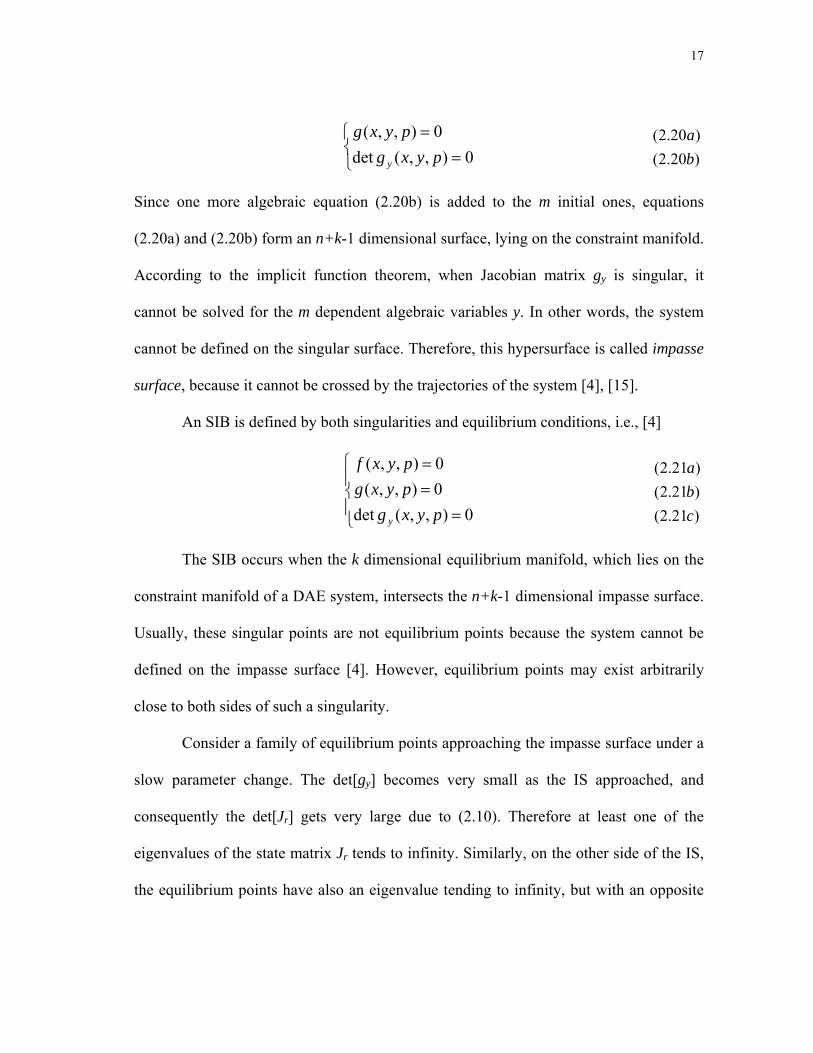
0),,(det0),,(pyxg

pyxg

y

)20.2()20.2(

ba

Since one more algebraic equation (2.20b) is added to the m initial ones, equations

(2.20a) and (2.20b) form an n+k-1 dimensional surface, lying on the constraint manifold.

According to the implicit function theorem, when Jacobian matrix gy is singular, it

cannot be solved for the m dependent algebraic variables y. In other words, the system

cannot be defined on the singular surface. Therefore, this hypersurface is called impasse

surface, because it cannot be crossed by the trajectories of the system [4], [15].

An SIB is defined by both singularities and equilibrium conditions, i.e., [4]

⎪⎩

⎪⎨

⎧

===

0),,(det0),,(0),,(

pyxgpyxgpyxf

y

)21.2()21.2()21.2(

cba

The SIB occurs when the k dimensional equilibrium manifold, which lies on the

constraint manifold of a DAE system, intersects the n+k-1 dimensional impasse surface.

Usually, these singular points are not equilibrium points because the system cannot be

defined on the impasse surface [4]. However, equilibrium points may exist arbitrarily

close to both sides of such a singularity.

Consider a family of equilibrium points approaching the impasse surface under a

slow parameter change. The det[gy] becomes very small as the IS approached, and

consequently the det[Jr] gets very large due to (2.10). Therefore at least one of the

eigenvalues of the state matrix Jr tends to infinity. Similarly, on the other side of the IS,

the equilibrium points have also an eigenvalue tending to infinity, but with an opposite

18

sign [1]. We have therefore a change of the stability properties of the system on the two

sides of the singularity and this constitutes a bifurcation, called singularity-induced

bifurcation [17], [22].

Note that in DAE systems the det[Jr] changes sign, either when it becomes

singular, having a zero eigenvalue, or when it has an unbounded eigenvalue going from

minus infinity to plus infinity [11], [21]. The previous one could be an SNB while an

SIB for the later one.

Let us take an example to illustrate SNB and SIB:

(2.22)2 pyxx +−=&

(2.23)10 22 pxyy −−+−=

ℜ⊂∈ℜ⊂∈ℜ⊂∈ PpYyXx ,,

where p is a positive scalar parameter. In this system, n=m=k=1. The state and

parameter space X, Y, P has dimension n+m+k=3. The constraint manifold is a surface

of dimension n+k=2. The impasse surface is an n+k-1=1 dimensional curve and the

equilibrium manifold is another k=1 dimensional curve lying on the constraint manifold.

The 2-dimensional constraint manifold, defined by (2.23), is represented through

a collection of contours shown in Fig. 5 with solid lines for different values of p. The

impasse surface (IS) is defined by the constraint (2.23) and the singularity condition

012 2 =−+−=∂∂

= xyygg y (2.24)

It is shown as a dash curve marked IS in Fig. 5 that divides the constraint manifold into

two components. Note that each solid curve of the constraint manifold folds with respect

19

to the x-axis at its crossing point with the impasse curve. The equilibrium manifold (EM)

satisfies the following conditions:

(2.25)02 =+− pyx

(2.26)01 22 =−−+− pxyy

From above two equations, we get the curve in X, Y space

(2.27)05.01 2 =−−+− xxy

which is shown as a dash-dot line marked EM in Fig. 5.

Fig. 5. C: singularity-induced bifurcation, B: saddle-node bifurcation.

20

As seen in Fig. 5, the equilibrium manifold EM intersects the impasse surface IS at point

C, which is a singularity-induced bifurcation. We use the reduced Jacobian matrix to

calculate eigenvalues in the bifurcation analysis. The linearized system around an

equilibrium point is expressed as below:

⎥⎦

⎤⎢⎣

⎡∆∆

=⎥⎥⎦

⎤

⎢⎢⎣

⎡∆yx

Jxu

0

.

(2.28)

(2.29)12

12

2 ⎥⎥

⎦

⎤

⎢⎢

⎣

⎡

−+−−

−−−

=

⎥⎦

⎤⎢⎣

⎡=

xyx

yxxy

ggff

Jyx

yxu

xJx r∆=∆& (2.30)

)31.2(

1121

2

2

2

1

⎟⎟⎠

⎞⎜⎜⎝

⎛

−−+−−−=

−= −

xyx

xyy

ggffJ xyyxr

The eigenvalue of the reduced Jacobian Jr just equals to Jr. Fig. 6 shows the eigenvalue

locus as p→0.125. We can see clearly that as p close to 0.125 from one side, say

p=0.125−, the eigenvalue of Jr tends to minus infinity; as p=0.125, gy is singular; after

this point, say p=0.125+, the eigenvalue of Jr tends to plus infinity. So the system

21

changes the property at p=0.125 which corresponds to the singularity-induced

bifurcation (SIB) point C.

-∞

+∞

Fig. 6. Singularity-induced bifurcation as p=0.125.

For this case we can also observe the saddle-node bifurcation. Now let p varies

slowly starting from 0 to seek SNB. For p=0 we have x=0, y=1. The eigenvalues of Ju

are –1, –1 while the eigenvalue of Jr is –1. This is a stable equilibrium point. Increasing

p slowly, we move uphill along the dash-dot equilibrium curve until reaching point B

(for p slightly larger than 0.1545), after which there is no equilibrium point for

increasing p. This is an SNB, at which a stable equilibrium point such as M coalesces

with an unstable equilibrium point such as N, which bounds the region of attraction of

the stable equilibrium point M. The descending path in the direction of N is made up of

unstable equilibria becoming more and more unstable with an eigenvalue approaching

22

+∞ at the SIB point C. There is no Hopf bifurcation since this is an n=1 dimensional

system. We will observe Hopf bifurcation through a simple power system example in

chapter III.

In conclusion, a bifurcation occurs when the qualitative structure of the system

(i.e., the number of equilibrium points, their stability, etc.) changes for a small variation

of the parameters. In the parameter dependent DAE problems, there are three generic

bifurcations [2], [17]:

• Saddle-node bifurcation (SNB), where two equilibria coalesce and then

disappear. At this point the Jacobian has a zero eigenvalue, i.e., it is singular.

• Hopf bifurcation (HB), where there is emergence of oscillatory instability. At

this point, two complex conjugate eigenvalues of Jacobian cross the imaginary axis.

• Singularity-induced bifurcation (SIB), where gy is singular. One eigenvalue is

going to infinity at both sides of the singular point with opposite sign.

2.3 Fundamental Insights of the Modeling Approaches

Dynamics may evolve in different time scales; some are fast and others slow. It

is not practical to treat both dynamics in the same way. For a DAE system, due to the

algebraic constraints, we cannot directly perform integration or calculate eigenvalues. In

this section, we introduce our new singular perturbation approach to solve DAE

systems. Our goal is to remodel the DAE system by an ODE without reductions. Hence

we can integrate directly to the ODE. The ODE should preserve bifurcation properties

of the original DAE system, since the bifurcations are the critical points to determine the

23

stability boundaries in the parameter-state space of X, Y, P [17]. We will demonstrate it

through a simple example.

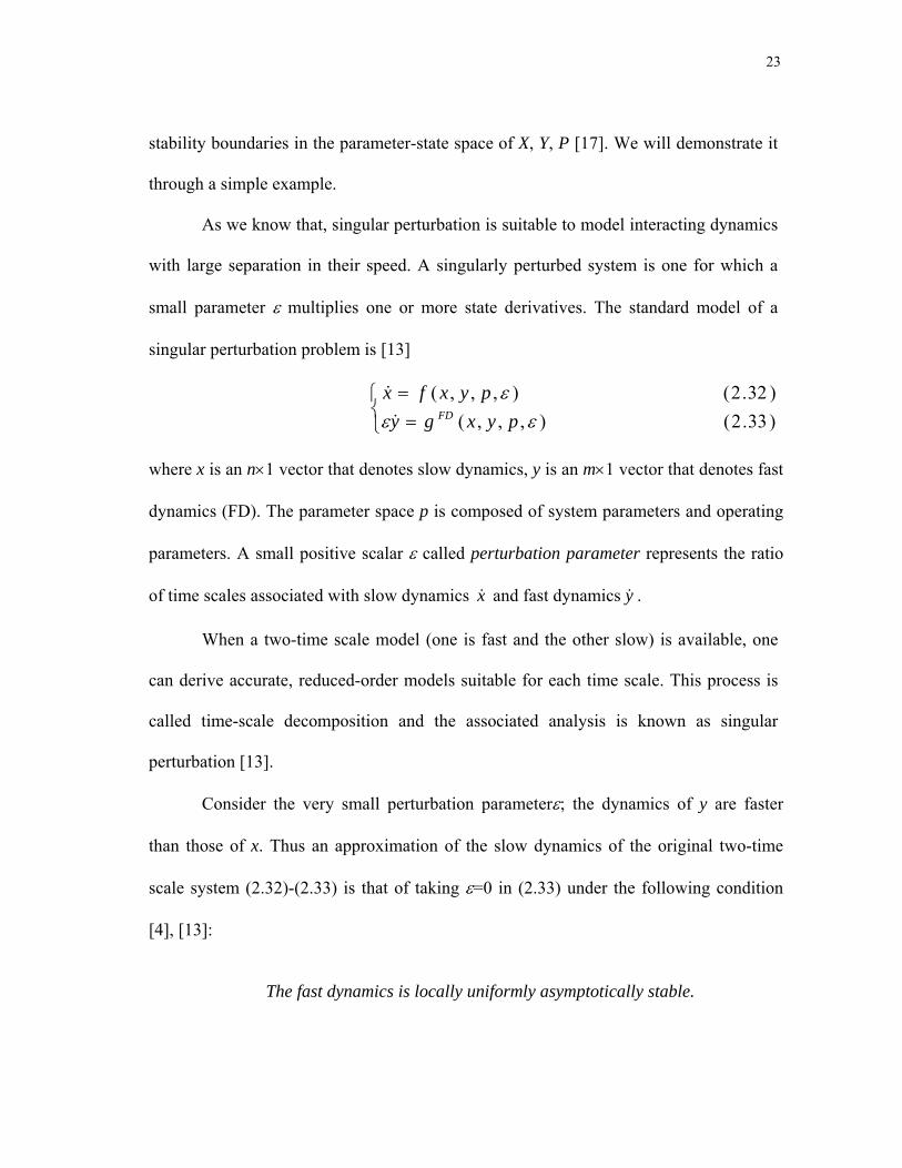
As we know that, singular perturbation is suitable to model interacting dynamics

with large separation in their speed. A singularly perturbed system is one for which a

small parameter ε multiplies one or more state derivatives. The standard model of a

singular perturbation problem is [13]

)33.2()32.2(

),,,(),,,(

⎩⎨⎧

==

εεεpyxgy

pyxfxFD&

&

where x is an n×1 vector that denotes slow dynamics, y is an m×1 vector that denotes fast

dynamics (FD). The parameter space p is composed of system parameters and operating

parameters. A small positive scalar ε called perturbation parameter represents the ratio

of time scales associated with slow dynamics x& and fast dynamics y& .

When a two-time scale model (one is fast and the other slow) is available, one

can derive accurate, reduced-order models suitable for each time scale. This process is

called time-scale decomposition and the associated analysis is known as singular

perturbation [13].

Consider the very small perturbation parameterε; the dynamics of y are faster

than those of x. Thus an approximation of the slow dynamics of the original two-time

scale system (2.32)-(2.33) is that of taking ε=0 in (2.33) under the following condition

[4], [13]:

The fast dynamics is locally uniformly asymptotically stable.

24

It means that FDyg (i.e. yg FD ∂∂ ) has all eigenvalues with strictly negative real parts,

i.e., fast modes converge. It also implies that Jacobian FDyg is nonsingular and all

trajectories remain in the attractive region of the stable equilibrium of the FDyg

dynamics. Under this condition, when 0=ε , the dynamics of y is infinitely faster than

those of x, the ODE (2.32)-(2.33) becomes DAE (2.34)-(2.35). The system order (n+m)

is then reduced to n, the order of x.

)35.2()34.2(

),,(0),,(

⎩⎨⎧

==

pyxgpyxfx

FD

&

The slow subsystem is a differential-algebraic system that can be analyzed through the

reduced Jacobian matrix Jr as described in the previous section. The slow subsystem

approximates the dynamics of the original ODE system (2.32)-(2.33) well [4], [13]; and

the dynamic behaviors of the system around an equilibrium point is characterized by the

reduced Jacobian matrix Jr of the form (2.10).

However, power system dynamic analysis has been based on the differential-

algebraic equations of the form (2.34)-(2.35). The algebraic constraints result from

approximating the fast dynamics as instantaneous variables. Obviously, the singular

perturbation approach is an inverse process to achieve our goal. However, we still can

apply the singular perturbation approach to introduce the fast dynamics, so that the DAE

comes back to the ODE without any reduction.

For general systems we formulate the problem as follows:

Given the differential-algebraic equations (DAE) of power system dynamics

25

)37.2()36.2(

),,(0),,(

⎩⎨⎧

==

pyxgpyxfx&

Convert the DAE to the singularly perturbed ODE

)39.2()38.2(

),,,(),,,(

⎩⎨⎧

==

εεεpyxgy

pyxfxFD&

&

Let us take an example to see why we want to do this.

2.3.1 A Simple Example of Using the Reduction Method

A DAE system is shown in (2.40a), (2.40b), and (2.40c):

⎪⎩

⎪⎨

⎧

ℜ⊂∈ℜ⊂∈ℜ⊂∈

−−+−=+−=

+++ )40.2(,,)40.2()40.2(

102

22

cPpYyXxba

pxyypyxx&

where p>0 is a scalar parameter and assumed slowly changing. Due to the algebraic

constraints (2.40b), we cannot directly integrate to find its dynamic response based on

the DAE. The reduction method solves for fast variable y from (2.40b) and substitutes it

in (2.40a), then integrate the remaining slow dynamics to obtain the trajectories of slow

variable x or calculate eigenvalues through the reduced Jacobian matrix Jr in bifurcation

analysis.

The equilibrium points of the above system satisfy

⎩⎨⎧

−−+−=+−=

)41.2()41.2(

1020

22 ba

pxyypyx

From (2.41b) we have two solutions of y for a given p:

26

2411 22 pxx

y−−+−

= (2.42a)

and

2411 22 pxx

y−−−−

= (2.42b)

Substituting (2.42a) or (2.42b) in (2.41a), and letting

pxpxx

pxf 22

411),(

22

1 +⎟⎟

⎠

⎞

⎜⎜

⎝

⎛ −−+−−= (2.43a)

and

pxpxx

pxf 22

411),(

22

2 +⎟⎟

⎠

⎞

⎜⎜

⎝

⎛ −−−−−= (2.43b)

the system equilibrium points are the solutions of f1=0 and f2=0. Fig. 7 and Fig. 8 show

the curves f1(x, p) and f2(x, p) for different values of p respectively. The points at which

the curves cross the zero line are the system equilibrium points. We see that there are two

equilibrium points for each value of p. When 0<p<0.125, one of the two comes from f1=0

and the other comes from f2=0. When 0.125<p<0.1545, both comes from f1=0. When

p>0.1545, no equilibrium point exists anymore.

Note, for this case, we can solve for y in terms of x explicitly. However, it is

impossible to do that for most of nonlinear algebraic equations. For this simple example,

we have two solutions of y and we have to deal with each of them respectively, which

makes it more complicated in the procedure of analysis.

27

0 0.1 0.2 0.3 0.4 0.5 0.6 0.7 0.8 0.9 1 -0.4

-0.2

0

0.2

x

-0.5 x (sqrt (1-x 2 )+ sqrt (1-x 2 -4 p))+ 2 p

p=0.08

p=0.125

p=0.14 p=0.1545

f1

Fig. 7. The curves of f1(x, p) for different values of p.

0 0 .1 0 .2 0 .3 0 .4 0 .5 0 .6 0 .7 0 .8 0 .9 1 -0 .1

-0 .05

0

0 .05

0 .1

0 .15

0 .2

0 .25

0 .3

x

-0.5 x (sq rt (1-x 2 )-sq rt(1-x 2 -4 p))+2 p

p=0 .08

p=0 .1545

p=0 .14

p=0 .125

f2

Fig. 8. The curves of f2(x, p) for different values of p.

28

Actually, these equilibrium points come from two differential equations in two

reduced models. Substituting (2.42a) or (2.42b) in (2.40a), we obtain the reduced models

in terms of slow dynamics accordingly:

pxpxx

x 22

411 22

+⎥⎥⎦

⎤

⎢⎢⎣

⎡ −−+−−=& (2.44a)

or

pxpxx

x 22

411 22

+⎥⎥⎦

⎤

⎢⎢⎣

⎡ −−−−−=& (2.44b)

The Jacobian matrices of the slow dynamics are as followings respectively:

2

22

22

411

11

21

2411

xpxx

pxxJ r

⎥⎥⎦

⎤

⎢⎢⎣

⎡

−−+

−+

⎥⎥⎦

⎤

⎢⎢⎣

⎡ −−+−−= (2.45a)

or

2

22

22

411

11

21

2411

xpxx

pxxJ r

⎥⎥⎦

⎤

⎢⎢⎣

⎡

−−−

−+

⎥⎥⎦

⎤

⎢⎢⎣

⎡ −−−−−= (2.45b)

As p varies, we can trace system equilibrium points and eigenvalues based on the

reduced models above. TABLE I shows the corresponding equilibrium points and

eigenvalues for different values of p:

29

TABLE I EQUILIBRIUM POINTS AND EIGENVALUES OF THE DAE SYSTEM

P

C+ component

pxpxx

x 22

411 22

+⎥⎥⎦

⎤

⎢⎢⎣

⎡ −−+−−=&

C_ component

pxpxx

x 22

411 22

+⎥⎥⎦

⎤

⎢⎢⎣

⎡ −−−−−=&

p=0.08

xe = 0.1789 ye = 0.8944 λ = −0.8583

xe = 0.8 ye = 0.2 λ = −1.2667

p=0.125−

xe = 0.3162 ye = 0.7906 λ = −0.6589

xe = 0.7071 ye = 0.3536 λ = −inf

p=0.125

SIB

p=0.125+

xe1 = 0.3162 ye1 = 0.7906 λ = −0.6589

xe2 = 0.7071 ye2 = 0.3536 λ = inf

No equilibrium point.

p=0.14

xe1 = 0.3818 ye1 = 0.7333 λ = −0.5201

xe2 = 0.6559 ye2 = 0.4269 λ = 2.0322

No equilibrium point.

p=0.1544

xe1 = 0.5138 ye1 = 0.6010 λ = −0.0634

xe2 = 0.5375 ye2 = 0.5745 λ = 0.0694

No equilibrium point.

p=0.1545 SNB

xe1 = xe2 = 0.5257 ye1 = ye2 = 0.5878

λ = 0 No equilibrium point.

p> 0.1545 No equilibrium point. No equilibrium point.

30

We also present the p-y curve in Fig. 9. Along the p-y curve, the segment B-C

corresponds to unstable equilibrium points while the others stable. This p-y curve is

similar to the P-V curve in power system literature where p corresponds to P, the active

power load; y corresponds to V, the load bus voltage.

Fig. 9. The p-y curve of the DAE system. B: saddle-node bifurcation, C: singularity-induced bifurcation.

From TABLE I and Fig. 9, we have the following observations:

• p=0.125 corresponds to an SIB (point C in Fig. 9), where two equilibrium

points, one to each side of C, have eigenvalues tending to infinity, but

with an opposite sign.

• p=0.1545 corresponds to an SNB (point B in Fig. 9), where two

equilibrium points, one stable and one unstable, coalesce and disappear

with zero eigenvalue.

31

• When 0<p<0.1545, there exist two equilibrium points of the system.

o When 0<p<0.125, two stable equilibrium points with two

differential equations. One of the two equilibrium points comes

from (2.43a) while the other one comes from (2.43b). Both

eigenvalues are less than zero.

o When 0.125<p<0.1545, two equilibrium points with the

differential equation (2.43a), one is stable, the other one unstable;

and equation (2.43b) has no equilibrium point.

• When p>0.1545, no equilibrium points exist anymore.

In the dynamic state and instantaneous state space, i.e. X, Y space, the 2-

dimensional constraint manifold, defined by (2.40b), is represented through a collection

of contours shown in Fig. 10 with solid lines for different values of p. As already known,

there is an SIB at point C as p=0.125. This SIB brings out the impasse surface (It is

shown as a dashed curve marked IS in Fig. 10) that divides the constraint manifold by

cut off on the tip into two components in the state space. The impasse curve is defined

by the singularity of the fast dynamics:

012 2 =−+−= xyg y (2.46)

32

Fig. 10. Two components C+ and C_ divided by IS. B: saddle-node bifurcation, C: singularity-induced bifurcation. The heavier lines represent the stability boundaries in C+ and C_ respectively.

The two components defined by (2.42a) and (2.42b) have their own dynamics

defined by (2.44a) and (2.44b) respectively. Each dynamics has its own stability region

in the state space. The two components are denoted here as C+ and C_ shown in Fig. 10

respectively. In Fig. 5, we can also see that the singularity-induced bifurcation point C

separates the p-y curve into the two components C+ and C_.

The equilibrium points satisfy the conditions (2.41a) and (2.41b). From the two

equations, we get the equilibrium manifold in X, Y space:

05.01 2 =−−+− xxy (2.47)

33

which is shown as a dash-dot curve marked EM in Fig. 10. Given p>0, the points at

which the constraint manifold intersects the EM are the system equilibrium points for the

specific value of p.

As seen in Fig. 10, when p=0.125, the equilibrium manifold EM together with

the constraint manifold intersects the impasse surface IS at point C, which is the

singularity-induced bifurcation. When p=0.1545, the equilibrium manifold EM tangents

the constraint manifold at point B, which is a saddle-node bifurcation. The SNB and SIB

are the critical points to determine the stability boundaries in parameter-state space.

Now, let us look into the region of attraction and the stability boundaries of the

stable equilibrium points for each dynamics in C+ and C_ respectively. Here we just

consider x, y, and p in ℜ+ space for simplicity.

On the C+ component

• When 0<p<0.125, there are two stable equilibrium points for each p that are

defined, respectively, by two different stable dynamic equations in the two

components C+ and C_, one to each side of the impasse surface IS (such as H in

C+ and L in C_, see Fig. 10). Because system states cannot be defined on the

impasse curve, the trajectories of the dynamics in C+ cannot cross the IS into C_,

and vice verse. Hence, the segment d-C along IS lies on the stability boundaries

of the stable equilibria in C+.

• When 0.125<p<0.1545, given p, we have two equilibrium points in C+, one stable

and one unstable (such as M and N as p=0.14, see Fig. 7). The unstable

equilibrium point bounds the stability region of the stable one. As p varies

34

between 0.125 and 0.1545, the collection of the stable equilibria in C+ consists of

the segment B-J along the EM curve while the collection of the unstable

equilibria in C+ consists of the segment C-B. Thus, the C-B segment lies on the

stability boundaries of the stable equilibria in C+. As 0.125<p<0.1545, the

descending path from B in the direction of N is made up of unstable equilibria

becoming more and more unstable with an eigenvalue approaching +∞ at the SIB

point C (see TABLE I).

• When p=0.1545, the saddle-node bifurcation occurs at point B. For the first order

differential equation, B is a saddle-node in the sense that near B there exists a

direction in the state space, along which trajectories behave as shown in Fig. 11,

approaching the equilibrium from one side, and diverging on the other. In this

case the system reaches the SNB by a gradual increase of p, the trajectory will

depart from the equilibrium surface along the unstable manifold (the B-D curve

in Fig. 10) of the SNB and it will end up on the impasse surface at point D which

is not an equilibrium point. Similarly, if p is larger than 0.1545, all the trajectories

will sink to the impasse curve along the corresponding constraint manifold (see

the trajectory as p=0.2 in Fig. 10), and the system collapses in the sense that no

equilibria exist anymore. Hence the B-a curve along the constraint manifold as

p=0.1545 lies on the stability boundaries in C+.

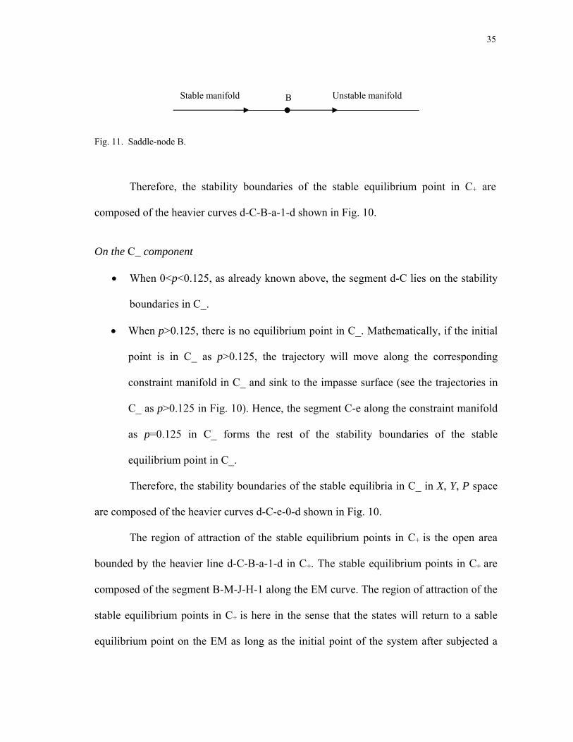
35

Fig. 11. Saddle-node B.

Therefore, the stability boundaries of the stable equilibrium point in C+ are

composed of the heavier curves d-C-B-a-1-d shown in Fig. 10.

On the C_ component

• When 0<p<0.125, as already known above, the segment d-C lies on the stability

boundaries in C_.

• When p>0.125, there is no equilibrium point in C_. Mathematically, if the initial

point is in C_ as p>0.125, the trajectory will move along the corresponding

constraint manifold in C_ and sink to the impasse surface (see the trajectories in

C_ as p>0.125 in Fig. 10). Hence, the segment C-e along the constraint manifold

as p=0.125 in C_ forms the rest of the stability boundaries of the stable

equilibrium point in C_.

Therefore, the stability boundaries of the stable equilibria in C_ in X, Y, P space

are composed of the heavier curves d-C-e-0-d shown in Fig. 10.

The region of attraction of the stable equilibrium points in C+ is the open area

bounded by the heavier line d-C-B-a-1-d in C+. The stable equilibrium points in C+ are

composed of the segment B-M-J-H-1 along the EM curve. The region of attraction of the

stable equilibrium points in C+ is here in the sense that the states will return to a sable

equilibrium point on the EM as long as the initial point of the system after subjected a

B Unstable manifold Stable manifold

36

small disturbance is within the region. For example, suppose the system is operating at

stable equilibrium point M as p=0.14 in C+. The initial point after subjected a small

disturbance is at point IM. For the specific value of p, the region of attraction of the stable

equilibrium point M is the curve along the corresponding constraint manifold above the

unstable equilibrium point N in C+. During the dynamic procedure, parameter p keeps

constant under the assumption that p is slowly changing. The system states keep staying

on the corresponding constraint manifold as p=0.14. Finally, the system trajectory will

return to M since IM is within the region of attraction of the stable equilibrium point M.

Likewise, the region of attraction of the stable equilibrium points in C_ is the

open area bounded by the heavier line d-C-e-0-d in C_. For example, as p=0.08 we have

a stable equilibrium point L in C_. If the initial point, upon clearing a small disturbance,

is at point IL within the region of attraction of the stable equilibrium point L, the system

trajectory will return to L along the constraint manifold. The third region bounded by e-

C-B-a-e contains no equilibria and all trajectories staying on constraint manifolds sink

into the impasse curve (see the trajectories as p=0.2 in Fig. 10), where the system is not

well defined and the event is unpredictable, resulting in the system collapse [17], [23].

As already known, the reduced models (2.44a) and (2.44b) represent the

dynamics in terms of slow variable x defined in C+ and C_ respectively. It is convenient

to observe the stability boundary in X state space by simply project it to the x-axis in Fig.

10. For instance, as p=0.14, we have two equilibrium points in C+ (see TABLE I and Fig.

10):

M: (xe1, ye1) = (xM, yM) = (0.3818, 0.7333)

37

and

N: (xe2, ye2) = (xN, yN) = (0.6559, 0.4269)

M is stable, and N is unstable. In X space, the stability boundary of the stable equilibrium

xe1 (i.e. xM in Fig. 10) is determined by the unstable equilibrium point xe2 (i.e. xN in Fig.

10), which is illustrated in Fig. 12. Given x0=0.5 (corresponding to initial point IM in Fig.

10) within the region of attraction of the stable equilibrium xM (=xe1), the time response

follows the path of (2.44a) and converges to the stable equilibrium point xM (see Fig. 13).

Fig. 12. Stability boundary in X space for p=0.14 in C+.

0 5 10 15 20 25 300.36

0.38

0.4

0.42

0.44

0.46

0.48

0.5

0.52

time (sec)

x

p=0.14, Slow Dynamics in C+

x

Fig. 13. Time response of (2.44a) converges to xM=xe1=0.3818. Initial x0=0.5.

xM xN 0

38

Similarly, as p=0.08, we have two stable equilibrium points H and L in C+ and C_

respectively (see TABLE I and Fig. 10):

H: (xe1, ye1) = (xH, yH) = (0.1789, 0.8944)

and

L: (xe2, ye2) = (xL, yL) = (0.8, 0.2)

Since the impasse curve intersects the corresponding constraint manifold as p=0.08 at

xQ=0.8246, the stability boundary of the stable equilibrium point xe2 (i.e. xL in Fig. 10) in

C_ in X space is determined by xQ (see Fig. 14). Note, the stability boundary of the stable

equilibrium point xe1 (i.e. xH in Fig. 10) in C+ in X space is also determined by xQ (see

Fig. 15).

Given x0=0.6 (corresponding to initial point IL in Fig. 10) within the region of

attraction of the stable equilibrium xL (=xe2), the time response follows the path of (2.44a)

and converges to the stable equilibrium point xL (see Fig. 16).

Fig. 14. Stability boundary in C_ in X space for p=0.08.

Fig. 15. Stability boundary in C+ in X space for p=0.08.

xL xQ 0

xH xQ 0

39

0 5 10 15 20 25 300.55

0.6

0.65

0.7

0.75

0.8

0.85

0.9

time (sec)

x

p=0.08 slow dynamics x in C_

Fig. 16. Time response of (2.44b) converges to xL=xe2=0.8. Initial x0=0.6.

As has been known, system trajectories that encounter impasse surface generally

cannot continue because the system cannot be defined on the singular point [4]. From the

engineering point of view, system can only work in one component with its dynamics

defined in the component, such as (2.44a) defined in C+ with wider region of attraction

for this case. The other one is then physically meaningless. In real power systems, the

equilibrium point in C_ is of too low bus voltage for operation. A system break up by

selective protection will follow. Therefore, we always let the power system dynamics

along the upper operating path in C+. Fig. 17 shows such a case of p=0.08 (refer to

TABLE I for the corresponding equilibrium points and eigenvalues) where the time

response for x0=0.7 (corresponding to initial point IH in Fig. 10) converges to the stable

equilibrium point xH = 0.1789.

40

0 5 10 15 20 25 300.1

0.2

0.3

0.4

0.5

0.6

0.7

0.8

time (sec)

x

x

p=0.08 slow dynamics in C+

Fig. 17. Time response of (2.44a) converges to xH=0.1789. Initial x0 = 0.7.

From above we see that the procedure of the reduction method to analyze

nonlinear DAE systems is quite complicated since we have to solve for y and deal with

the two solutions of y and the two reduced slow dynamics of x respectively, which only

gives local pictures of system behaviors. In the next section, we will discuss a singularly

perturbed ODE form that well descries the original DAE system. Through the ODE, we

avoid solving the nonlinear algebraic equations and directly perform integration without

reduction process.

2.3.2 A Simple Example to Demonstrate Our New Singularly Perturbed ODE

Let us look into the singularly perturbed ODE. We put the original DAE here for

convenience:

41

)50.2()49.2()48.2(

,,10

222

⎪⎩

⎪⎨

⎧

ℜ⊂∈ℜ⊂∈ℜ⊂∈

−−+−=+−=

+++ PpYyXxpxyy

pyxx&

Suppose the singularly perturbed ODE is expressed as below:

)52.2()51.2(

121

2

2

22

⎪⎩

⎪⎨

⎧

⎟⎟⎠

⎞⎜⎜⎝

⎛

−+−

−−+−−=

+−=

xypxyyy

pyxx

&

&

ε

where ε is the perturbation parameter and the Jacobian of algebraic equations is

nonsingular, i.e.

012 2 ≠−+−= xyg y (2.53)

The original DAE system is essentially approximated by a set of ODEs with an attractive

manifold given by the algebraic constraint equations. The requirements of applying the

singularly perturbed ODE will be discussed in the next section. The technique to convert

a DAE to a singularly perturbed ODE will be introduced in chapter III. Here we just use

the ODE and compare with the original DAE to analyze the system dynamics.

Once the singularly perturbed ODE is obtained, the time domain simulations or

complex domain bifurcation analysis can be performed directly to this explicit state

space form without any reductions.

The state x, y can be anywhere in the state space since there is no constraint

manifold in the singularly perturbed ODE.

The equilibrium points of the ODE system follow the equations:

42

)55.2()54.2(

12

10

20

2

22

⎪⎩

⎪⎨

⎧

⎟⎟⎠

⎞⎜⎜⎝

⎛

−+−

−−+−−=

+−=

xy

pxyypyx

Under the condition of (2.53), we get the same solutions of equilibrium points as the

DAE:

)57.2()56.2(

1020

22⎩⎨⎧

−−+−=+−=

pxyypyx

Thus in X, Y space, we have the same equilibrium manifold as DAE:

05.01 2 =−−+− xxy (2.58)

which is shown as a dash-dot curve marked EM in Fig. 18.

From (2.53) we also have the same impasse curve as the DAE defined by the

singular surface:

012 2 =−+−= xyg y (2.59)

All the trajectories of the ODE system cannot cross the impasse surface. Like we

mentioned in section 2.3.1, the impasse curve marked IS in Fig. 18 divides the state

space into two components C+ and C_ and the dynamics of the ODE system are defined

in the two components. Note, due to (2.50), the ODE system is defined with the

limitation of 0<x<1, so that the two components are the open areas C+ and C_ left to the

line x=1. Since the algebraic equations are approximated by the fast dynamics (2.52), the

instantaneous algebraic variable y becomes fast dynamic state y. Hence, the states x and y

can be anywhere in the state space. The trajectories of the states x, y will follow the

dynamics (2.51)-(2.52) and converge fast to the algebraic constraints in some local

43

neighborhood of the exact solution. This dynamic behavior of the ODE can be directly

observed from phase portraits in phase plan, where the system dynamics are augmented

in the state space through the recovery of fast dynamics. We will demonstrate it later on.

Fig. 18. The singularly perturbed ODE defined in components C+ and C_. B: saddle-node bifurcation, C:

singularity-induced bifurcation.

To analyze the dynamic behaviors of the ODE system, we solve for system

equilibrium points for each given p. All the equilibrium points will be on the equilibrium

manifold. The eigenvalues for each of the equilibrium points are calculated using the

following unreduced Jacobian matrix:

44

⎥⎥⎥

⎦

⎤

⎢⎢⎢

⎣

⎡

−−−+−

−

−−=

εε1

1)12(1

22 xxyx

xyJu (2.60)

where Ju is built in certain simplifications. We will discuss the system Jacobian of the

ODE in detail in chapter III. As p varies, we trace system equilibrium points and

eigenvalues based on (2.56), (2.57), and (2.60). TABLE II shows the corresponding

equilibrium points and eigenvalues for different values of p.

Compared with the original DAE, the eigenvalue λ1 of the unreduced Jacobian Ju

is quite similar to the eigenvalue λ of the reduced Jacobian Jr. The negative λ2 with large

magnitude represents the very fast convergence of the fast dynamics.

We have already known that the original DAE has two bifurcations an SNB and

an SIB. From TABLE II we see that the singularly perturbed ODE preserves the

bifurcation properties of the original DAE system. The two bifurcations marked B and C

respectively are shown in Fig. 18. In Fig. 19, we see that the singularity-induced

bifurcation point C separates the p-y curve into the two components C+ and C_. Along the

p-y curve, segment B-C corresponds to unstable equilibrium points while the others

stable. This feature is just the same as the demonstrated in Fig. 9 for the DAE system in

section 2.3.1.

45

TABLE II EQUILIBRIUM POINTS AND EIGENVALUES OF THE ODE SYSTEM COMPARED WITH THE

ORIGINAL DAE SYSTEM

Original DAE Singularly perturbed ODE p

C+ component C_ component C+ component C_ component

p=0.08

xe = 0.1789 ye = 0.8944 λ = −0.8583

xe = 0.8 ye = 0.2

λ = −1.2667

xe = 0.1789 ye = 0.8944 λ1 = −0.8583

λ2 = −100000.0361

xe = 0.8 ye = 0.2

λ1 = −1.2667 λ2 = −99998.9333

p=0.125−

xe = 0.3162 ye = 0.7906 λ = −0.6589

xe = 0.7071 ye = 0.3536 λ = −inf

xe = 0.3162 ye = 0.7906 λ1 = −0.6588

λ2 = −100000.1318

xe = 0.7071 ye = 0.3536 λ1 = −inf λ2 = −inf

p=0.125

SIB

p=0.125+

xe1 = 0.3162 ye1 = 0.7906 λ = −0.6589

xe2 = 0.7071 ye2 = 0.3536 λ = inf

No equilibrium point.

xe1 = 0.3162 ye1 = 0.7906 λ1 = −0.6588

λ2 = −100000.1317

xe2 = 0.7071 ye2 = 0.3536 λ1 = inf λ2 = −inf

No equilibrium point.

p=0.14

xe1 = 0.3818 ye1 = 0.7333 λ = −0.5201

xe2 = 0.6559 ye2 = 0.4269 λ = 2.0322

No equilibrium point.

xe1 = 0.3818 ye1 = 0.7333 λ1 = −0.5201

λ2 = −100000.2132

xe2 = 0.6559 ye2 = 0.4269 λ1 = 2.0322

λ2 = −100002.4590

No equilibrium point.

p=0.1545 SNB

xe1 = xe2 =0.5257 ye1 = ye2 =0.5878

λ = 0

No equilibrium point.

xe1 = xe2 =0.5257 ye1 = ye2 =0.5878

λ1=0 λ2= −100000.5878

No equilibrium point.

p> 0.1545 No equilibrium point.

No equilibrium point.

No equilibrium point.

No equilibrium point.

46

Fig. 19. The p-y curve of the ODE system. B: saddle-node bifurcation, C: singularity-induced bifurcation.

Now, let us look into the stability boundaries of the stable equilibrium point in

the phase plane of the state space.

When 0<p<0.125, we have two stable equilibrium points, say H and L as p=0.08,

in C+ and C_ respectively. See Fig. 20. Suppose the initial point is at point IH in C+

component. Upon clearing a disturbance, the system dynamics will converge very fast to

the corresponding constraint manifold and return to the stable equilibrium point H along

the constraint manifold. As p=0.08, the constraint manifold intersects the impasse curve

at point Q. Thus, the vertical line (x=0.8246) passing though Q together with the impasse

curve left to point Q consists of the stability boundaries of the stable equilibrium points

H and L in C+ and C_ respectively (marked heavier lines in Fig. 20). It is therefore, the

region of attraction of the stable equilibrium point H in C+ is the open area above the

stability boundaries in C+.

47

Fig. 20. Phase portrait as p=0.08. H: stable equilibrium point in C+, L: stable equilibrium point in C_, B:

saddle-node bifurcation, C: singularity-induced bifurcation.

Similarly, the region of attraction of the stable equilibrium point L in C_ is the

open area below the stability boundaries in C_. This phase portrait also reflects the “slow

down” of the fast dynamics through the small perturbation parameter ε (here ε=10-5). If

ε=0, the region of attraction will instantaneously shrink, in the y direction, to the

constraint manifold that associates the DAE model. The trajectories for the initial point

outside the region of attraction will sink to the impasse surface and the system collapses.

48

By projecting the phase plane to x-axis, we obtain the stability boundaries of the

stable equilibrium point H and L in X space shown in Fig. 21 and Fig. 22 respectively,

which are the same as the DAE model. Suppose the initial point is at IH: (x0, y0)=(0.7,

0.5) within the region of attraction of the stable equilibrium point H in C+, the time

responses of states x, y are shown in Fig. 23 where the trajectories approach to H. If the

initial point is at IL: (x0, y0)=(0.6, 0.33) within the region of attraction of the stable

equilibrium point L in C_, the time responses of states x, y are shown in Fig. 24 where

the trajectories approach to L. All the trajectories are obtained by directly integrating the

singularly perturbed ODE without substitutions and reductions like we did for the DAE

in section 2.3.1.

Fig. 21. Stability boundary of the stable equilibrium point H in C+ in X space as p=0.08.

Fig. 22. Stability boundary of the stable equilibrium point L in C_ in X space as p=0.08.

xL xQ 0

xH xQ 0

49

Fig. 23. Time response converges to H: (xH, yH)=(0.8944, 0.1789). Initial at IH: (x0, y0)=(0.7, 0.5) in C+ and

p=0.08.

Fig. 24. Time response converges to L: (xL, yL)=(0.8, 0.2). Initial at IL: (x0, y0)=(0.6, 0.33) in C_ and

p=0.08.

50

As p increases slowly to p=0.125, the singularity-induced bifurcation point C

occurs and no equilibrium point exists in C_. All the trajectories with initial point in C_

either sink to the impasse curve or to the SIB point C along the constraint manifold and

eventually the system collapses. On the other hand, the system may work at the stable

equilibrium point J in C+ component as p=0.125. The phase portrait and the region of

attraction of the stable equilibrium point J are shown in Fig. 25.

Fig. 25. Phase portrait as p=0.125. J: stable equilibrium point, C: singularity-induced bifurcation.

When 0.125<p<0.1545, we have two equilibrium points in C+, one stable and one

unstable, such as M and N as p=0.14 shown in Fig. 26. The unstable equilibrium point

determines the stability boundaries of the stable one. In Fig. 26, the region of attraction

51

of the stable equilibrium point M is the open area above the impasse curve and left to

line x=0.6559.

Fig. 26. Phase portrait as p=0.14. M: stable equilibrium point, N: unstable equilibrium point.

When p reaches 0.1545, a saddle-node bifurcation occurs at point B, where two

equilibria meet and disappear with a zero eigenvalue. In this case the system reaches the

SNB by a gradual increase of p, the trajectory will depart from the equilibrium surface

along the B-D curve (see Fig. 27) and it will end up on the impasse surface at point D,

which is not an equilibrium point. When p is lager than or equal to 0.1545, no stability

region exists anymore. All the trajectories will sink to the impasse curve and the system

get collapse.

52

Fig. 27. Phase portrait as p≥0.1545. B: saddle-node bifurcation.

This example illustrates that we can observe time domain trajectories by directly

integrating the singularly perturbed ODE without reduction computation. The ODE

presented above preserves the bifurcation properties of the original DAE system. Since

the fast dynamics is introduced, the instantaneous variable y becomes fast dynamic state

y. Here the perturbation parameter ε plays the role to slow down the fast dynamics to

observe. The slow state x and fast state y are no longer confined in the constraint

manifold for all time. In other words, x and y can be anywhere in the state space. The

components C+ and C_ in which the ODE dynamics is defined are augmented with

respect to fast state y. The stability region is therefore augmented in X, Y state space.

Look into the phase portraits above, we see that the system dynamics converge very fast

53

to the algebraic constraints or to the impasse surface: when left to the tip point on the

constraint manifold (at which the constraint manifold is cut off by the impasse curve),

the impasse curve is kind of a source and all the trajectories depart from the impasse

curve and converge very fast to the constraint manifold; when right to the tip point, the

impasse curve is kind of a sink and all the trajectories move up or down to the impasse

curve and eventually the system collapse in the sense that the system is not well defined

on the impasse surface; when ε=0, the states instantaneously shrink, in the y direction,

to the constraint manifolds of the DAE model. In conclusion, the augmentation of

stability region is associated with fast state y. The stability boundaries and therefore the

regions of attraction of stable equilibrium points in X state space keep the same as the

original DAE system.

Through this example we see that the original DAE system is well descried by

the singularly perturbed ODE. However, there still exist issues need to investigate: What

are the requirements of using our singularly perturbed ODE? What are the complexities

in the procedure of building fast dynamics? We will address these issues in detail in the

coming sections.

2.4 The Requirements of Using the Singularly Perturbed ODE

To apply our new modeling approach, we need to investigate the requirements

under which the DAE (2.36)-(2.37) can be successfully converted to the singularly

perturbed ODE (2.38)-(2.39).

Three issues are discussed for our new singularly perturbed ODE:

54

2.4.1 ),,,( εpyxg FD Describing the Fast Dynamics Is Not Necessary the Same As

),,( pyxg

For a valid approximation the fast dynamics must converge [13]; i.e., its

eigenvalues must have negative real parts. However, this may not be true for the original

algebraic constraints 0=g(x, y, p). For example, consider the original DAE system

described by

)61.2()61.2(

02

ba

yxyxx

⎩⎨⎧

+−=+−=&

The reduced Jacobian matrix Jr is

1)1(2 −=−−−=rJ (2.62)

The eigenvalue of Jr is

1)( −=rJeig (2.63)

The system is dynamic stable. But if we introduce the fast dynamics by simply setting

),,,( εpyxg FD = ),,( pyxg , we get

)65.2()64.2(2

⎩⎨⎧

+−=+−=

yxyyxx

&

&

ε

Then, the unreduced Jacobian matrix Ju is

⎥⎥⎦

⎤

⎢⎢⎣

⎡−

−=

εε1112

uJ (2.66)

The eigenvalues of Ju can be obtained by solve the following equation:

55

01112

=−

−+

ελ

ε

λ

They are

04

11211 21 >+++−=

εελ (2.67)

04

11211 22 <+−+−=

εελ (2.68)

For any ε>0, we have eigenvalue λ1>0. Therefore, the dynamic system (2.64)-(2.65) is

unstable. It is clear that these two systems are totally different. The reason is that the fast

dynamics ),,,( εpyxg FD is diverging, since the Jacobian of the fast dynamics

εεε1)(11

=∂+−∂

=∂∂

=∂∂

yyx

yg

yg FD

(2.69)

has a positive eigenvalue

01)( >=∂∂

εygeig (2.70)

2.4.2 Fast Dynamics Has Eigenvalues with Larger Real Magnitude than That of Slow

Dynamics

According to the fundamental linear control theory, the dynamic response

depends on system characteristic root (i.e. eigenvalues) locations. If the roots are located

far away from the imaging axis in the open left half complex plane, the converging

response will be fast; and the slower it will be when approaching imaging axis.

56

Consider a standard second order linear system:

22

2

2)(

nn

n

ssG

ωςωω

++= (2.71)

The characteristic equation is

02 22 =++ nns ωςω (2.72)

The characteristic roots are

22,1 1 ςωςω −±−= nn js (2.73)

The under damped response (ζ<1) to a unit step input, subject to zero initial condition, is

given by

)1sin(1

1)( 2

2θςω

ς

ςω

+−−

−=−

tetc n

tn

(2.74)

Where

⎟⎟

⎠

⎞

⎜⎜

⎝

⎛ −= −

ςς

θ2

1 1tan (2.75)

It is straightforward to see that the dynamic settle time mainly determined by

nςω− , the real part of the characteristic roots. For the second-order system, the response

remains within 2 percent after 4 times constants, that is

nst ςω

4= (2.76)

This suggests that the perturbation parameter ε need to be small enough to guarantee the

fast dynamics converge fast. Again from above example (2.64)-(2.68), Let ε=10-5, then

57

eigenvalue λ1=99999.00001 in (2.67) corresponds to the fast dynamics, while

λ2=−1.00001 in (2.68) corresponds to the slow dynamics.

2.4.3 0),,,( =εpyxg FD if and only if 0),,( =pyxg

According to the singularly perturbed ODE, if fast dynamics ),,,( εpyxg FD of

(2.39) converges fast enough, then by taking ε=0 we can obtain a DAE system of the

form (2.36)-(2.37). Since the singular perturbation approach is an inverse process of

converting DAE to ODE, the ODE system (2.38)-(2.39) must approximate the original

DAE system (2.36)-(2.37) well. Comparing these two systems, we know immediately

that 0),,,( =εpyxg FD if and only if 0),,,( =εpyxg .

Now, according to above investigations, we have the following requirement to

build the fast dynamics:

Fast dynamics converge fast to the algebraic constraints.

The singularly perturbed ODE is suitable for numerical integration to obtain time

domain responses of dynamic systems. Based on the ODE, an unreduced Jacobian is also

used in eigenvalue analysis, which should preserve the bifurcation properties of the

original DAE systems. The detailed modeling technique will be described in chapter III.

58

2.5 Complexities of Building Fast Dynamics

From FDgy =&ε we know that the system will have different dynamic behaviors

for different value of ε. When ε is close to zero, there are different instantaneous variable

sequences can be employed to express the fast dynamics; In addition, g=0 implies –g=0.

And also there exists a question of if the singular perturbation preserves the bifurcation

properties of the original DAE system. These turn out complexities in building fast

dynamics.

2.5.1 The Selection of ε

We introduce the perturbation parameter ε to slow down the fast dynamics.

However, there are no explicit criteria to determine the value of ε need to ensure that the

trajectories fast enough converge to the constraint manifolds. In addition, the error

between the original DAE and the singularly perturbed ODE is related to ε. However,

there is no explicit expression of bounding the approximation error [12]. In our

applications, we select a small epsilon, say ε=10-5. It shows that this ε is small enough to

make the dynamic behavior of the singularly perturbed ODE system similar to the

original DAE system.

2.5.2 The Different Sequences of Fast Dynamic States y&

Consider two ODEs with different sequences of fast dynamic states shown below

59

⎥⎥⎥

⎦

⎤

⎢⎢⎢

⎣

⎡

⎥⎥⎥

⎦

⎤

⎢⎢⎢

⎣

⎡

−−

−=

⎥⎥⎥

⎦

⎤

⎢⎢⎢

⎣

⎡

2

1

1

2

1

1

300221011

yyx

yyx

&

&

&

εε (2.77)

⎥⎥⎥

⎦

⎤

⎢⎢⎢

⎣

⎡

⎥⎥⎥

⎦

⎤

⎢⎢⎢

⎣

⎡

−−

−=

⎥⎥⎥

⎦

⎤

⎢⎢⎢

⎣

⎡

2

1

1

1

2

1

300221011

yyx

yyx

&

&

&

εε (2.78)

As ε is close to zero, both (2.77) and (2.78) are approximated by DAE (2.79). But the

results of eigenvalue analysis shown in TABLE III are quite different.

⎥⎥⎥

⎦

⎤

⎢⎢⎢

⎣

⎡

⎥⎥⎥

⎦

⎤

⎢⎢⎢

⎣

⎡

−−

−=

⎥⎥⎥

⎦

⎤

⎢⎢⎢

⎣

⎡

2

1

11

300221011

00

yyxx&

(2.79)

TABLE III

EIGENVALUES OF THE THREE SYSTEMS (ε=0.001)

ODE (2.77) ODE (2.78) DAE (2.79)

-0.5

-2000.5

-3000.0

-0.5

3645.6

-1646.1

-0.5

The ODE system (2.77) is stable that matches the DAE system (2.79), while the ODE

system (2.78) unstable. The actual system Jacobian matrix of ODE (2.77) is

⎥⎥⎥

⎦

⎤

⎢⎢⎢

⎣

⎡

−−

−

εεεε

/2/2/1/300

011 (2.80)

Obviously the fast modes diverge because one of its eigenvalues ε)71( ± is large than

zero. The selection of the sequence depends on the fact that fast dynamics converge. So

60

we could not use the sequence shown in (2.77). For a system with m algebraic equations,

there will be !m different sequences to express the fast dynamics y& . However, there are

no easy criteria to verify which one satisfies the fast convergence requirement.

2.5.3 The Sign Adjustment of Algebraic Equations

We noted that the algebraic equation g(x,y,p)=0 implies −g(x,y,p)=0. For one-

dimensional algebraic constraint, the eigenvalue of Jr equals to Jr itself. Therefore, to

guarantee the fast dynamics converge, one may just set gFD=g or gFD= –g. There is an

overhead in the decision to switch between these two options. For a DAE with m

algebraic equations, there will be 2m possibilities of different sign. However, there is no

way to always guarantee fast modes converge by exhausting all the 2m possibilities.

TABLE IV shows that a 2-dimensional fast mode Jacobian has this scenario.

TABLE IV SIGN ADJUSTMENT FOR m=2

Fast Mode Jacobian ⎥

⎦

⎤⎢⎣

⎡1221

⎥⎦

⎤⎢⎣

⎡−− 1221

⎥⎦

⎤⎢⎣

⎡−−−−

1221

⎥⎦

⎤⎢⎣

⎡ −−1221

Eigenvalues -1

3

1.7321j

-1.7321j

-3

1

1.7321j

-1.7321j

61

2.5.4 The Singularly Perturbed ODE Is Not Necessary To Preserve the Bifurcation

Properties of the Original DAE System

Fast convergence of fast dynamics is the requirement of using our new modeling

approach to build fast dynamics. Singularly perturbed ODE form is valid only in the

approximation sense. This implies that a singularly perturbed ODE is not necessary to

preserve the bifurcation properties of the original DAE system, such as losing the

significance of the singularity-induced bifurcation of the original DAE system. We will

demonstrate this scenario in chapter III through a power system example.

2.6 Summary

In this chapter, we give fundamental insights on our modeling approaches.

Through a simple example, a detailed dynamic analysis of using reduction method is

demonstrated and compared with the singularly perturbed ODE. We can directly

integrate the ODE to quickly view the local dynamic behaviors of the system through

time responses. As has been seen, the singularly perturbed ODE makes it easier to

analyze since we do not need solving the nonlinear algebraic equations. The bifurcation

prosperities of the original DAE are preserved by the ODE.

We also discussed the requirements and the complexities of applying our new

modeling approach. The requirement is

Fast dynamics converge fast to the algebraic constraints.

62

Therefore, we need new design methods to satisfy the fast convergence

requirement to remodel a DAE by a singularly perturbed ODE, which is suitable for time

domain simulation and preserve the bifurcation properties of the original DAE system.

63

CHAPTER III

THE TECHNIQUE OF PTE: PERTURB AND TAYLOR’S EXPANSION

In this chapter, we propose PTE technique to convert a DAE to a singularly

perturbed ODE. Time domain simulation is then easily performed to this ODE to

observe dynamic responses. A simplified unreduced Jacobian matrix of the ODE is

introduced to perform eigenvalue analysis. Simulation results show that PTE technique

satisfies the fast convergence requirement and preserves the bifurcation properties of the

original DAE system. We will demonstrate PTE through a rudimentary power system

example.

3.1 Describe Fast Dynamics by PTE

We convert DAE (3.1)-(3.2)

⎩⎨⎧

==

),,(0),,(

pyxgpyxfx&

)2.3()1.3(

to a singularly perturbed ODE (3.3)-(3.4)

⎩⎨⎧

==

),,,(),,,(

εεε

pyxgypyxfx

FD&

&

)4.3()3.3(

Fast dynamics described by gFD needs to converge to the algebraic constraint g=0

fast to make our approximation meaningful. Under this condition, the simulation results

obtained from the ODE will have similar behaviors as the original DAE. Since

64

0),,( =pyxg is known, to get the fast dynamics of instantaneous variable y, we simply

perturb it around the algebraic constraint by a small positive scalar ε,

),,(0 pyyxg &ε+= (3.5)

By Taylor’s expansion we have

)(),,(),,(0 εε oypyxgpyxg y ++= & (3.6)

Ignoring high order terms we have

),,(),,( pyxgypyxg y −=&ε (3.7)

If gy is nonsingular, then

),,(),,( 1 pyxgpyxgy y−−=&ε (3.8)

Thus

gggy yFD 111 −−==

εε& (3.9)

Equation (3.9) gives a generic expression of fast dynamics. Therefore, the

singularly perturbed ODE obtained by PTE is as below:

⎪⎩

⎪⎨⎧

−=

=− ggy

pyxfx

y11

),,,(

ε

ε

&

&

)11.3()10.3(

The corresponding Jacobian matrix is given in (3.12):

⎥⎥

⎦

⎤

⎢⎢

⎣

⎡= FD

yFDx

yx

u gg

ffJ

εε11 (3.12)

For eigenvalue analysis, we evaluate Ju at each equilibrium point. From (3.9) we have

ggg FDy −= (3.13)

65

Taking the partial derivatives of the above equation in terms of x and y, we have

yFDyy

FDyy ggggg −=+ (3.14)

xFDxy

FDyx ggggg −=+ (3.15)

When gy is nonsingular, substituting gFD with –gy-1g into above equations, we obtain

yFDyyyyy gggggg −=+− − 1 (3.16)

xFDxyyyx gggggg −=+− − 1 (3.17)

At each equilibrium point where g=0, the above two equations become

mmyyFDy Iggg ×

− −=−= 1 (3.18)

xyFDx ggg 1−−= (3.19)

Or

mmFDy Ig ×−=

εε11

(3.20)

xyFDx ggg 111 −−=

εε (3.21)

where I is an m×m identity matrix. Obviously, (3.20) assures that fast dynamics always

converge fast since all its eigenvalues are ε1− . Thus the unreduced Jacobian Ju

becomes

⎥⎥

⎦

⎤

⎢⎢

⎣

⎡

−−=

×−

mmxy

yx

u Igg

ffJ

εε11 1 (3.22)

For a large-scale power system, m can be huge, so Ju is a sparse matrix. Then we can use

sparse techniques to compute its eigenvalues. On the contrary, a reduced Jacobian matrix

66

is not sparse and the solution efficiency is poor. For large power systems, the solution

time is increased significantly [20].

In (3.22), it seems that we need to calculate the inverse of gy to obtain Ju. But

since 1−yg is involved only in xy gg 11 −−

ε, an alternative way to avoid the inverse

calculation is as below:

From

xyFDx ggg 1−−= (3.23)

We have

xFDxy ggg −= (3.24)

Here gx, gy are known at each operating point. So we can obtain the matrix multiplication

of (3.23) by solving sparse linear equation of (3.24) under the assumption of a

nonsingular gy.

If gy is singular, we cannot solve for FDxg uniquely or the solution may not exist.

To handle this singularity, we apply perturbation technique again to get an approximate

unique solution of FDxg . At this time we perturb gy at the singular point by a small

positive scalar ε1, thus (3.7) becomes

gyIg y −=+ &)( 1εε (3.25)

Rewrite (3.25) by

gyIg y −=+ &)( µε (3.26)

67

where µ=ε1/ε. Therefore (gy+µI) is regularized by choosing µ=o(ε). We can solve for

FDxg by

xFDxy ggIg −=+ )( µ (3.27)

Hence, we can apply the PTE to describe a DAE by a singularly perturbed ODE.

Dynamic analysis can then be performed to the ODE without reduction calculation. We

can directly integrate slow dynamics x& and fast dynamics y& to obtain the time domain

trajectories. To perform eigenvalue analysis, we calculate eigenvalues using the

simplified unreduced Jacobian (3.22) and the bifurcation properties of the original DAE

system are preserved by PTE.

Note that for the original DAE, the singularity of the Jacobian of algebraic

equations (gy=0) brings out the impasse surface lying on the constraint manifolds defined

by (3.2). This impasse surface still exists in the singularly perturbed ODE. Under the

assumption of gy nonlinear, the equilibrium points of the ODE are the same as the DAE.

We calculate system equilibrium points through the equations the same as the DAE:

⎩⎨⎧

==

),,(0),,(0

pyxgpyxf

)29.3()28.3(

3.2 Case Study

In this section, we will apply PTE technique to a simple power system example.

We will compare the simulation results with those of the reduction method. We focus

on the dynamic voltage stability issues for this case.

68

3.2.1 Apply PTE to a Simple Power System

The simplified model shown in Fig. 28 retains the rudiments of power system

voltage dynamics, i.e., generator, voltage control, transmission and load [17].

Fig. 28. A two-bus power system.

This simplified model includes a one-axis generator model and a first-degree

simplification of the IEEE Type I excitation control [24] (refer to [17] for more details

on the modeling assumptions). The following parameter dependent differential-algebraic

equations describe the dynamics:

Dynamic Equations:

⎥⎦

⎤⎢⎣

⎡+

′′+−

+′+

−=′•

fdddd

d

EE

QxEx

xxEx

xxT

E2

0 ''

''1 (3.30)

⎥⎦⎤

⎢⎣⎡ −++−−−=

•

))()(1()(1 2220 rfdfdfd EExQxP

EKEE

TE (3.31)

Algebraic Equation:

EG

Control

Generator

EG,δG

Transmission ', dd xx

rE

θ,fdE

δ ′′,E PG+jQG

δ,E

Load P+jQ

x

Exciter

69

22222 )()(0 EQxPxEE +′−′−′= (3.32)

where Er is the set-point voltage, 0fdE is the nominal field excitation, and T, K are

control coefficients. The other notations are conventional. Equations (3.30)-(3.31)

denote the dynamics of the excitation system, the slow state variable x={E’, Efd}.

Equation (3.32) denotes the power flow of the system, the fast variable y={E}. The

parameter p can be the load p={P, Q} which is treated as constant power load. This is a

DAE model with two first-order differential equations (n=2) and one algebraic constraint

(m=1). The unreduced Jacobian is a 3×3 dimensional matrix. We select ε=10-5 and

consider the system defined in ℜ+ space. The parameters of the system are:

0.1,5.2,5.0,'',1.0

,2.0',2.1,6.1,5.1,5' 00

===+==

=====

rd

ddfdd

EKPQxxxx

xxETT

Let

⎥⎦

⎤⎢⎣

⎡+

′′+−

+′+

−= fdddd

dfd E

EQxE

xxxE

xxx

TPEEEf

2

01 '

'''

1),,,'( (3.33)

⎭⎬⎫

⎩⎨⎧

⎥⎦⎤

⎢⎣⎡ −++−−−= rfdfdfd EExQxP

EKEE

TPEEEf 222

02 )()(1)(1),,,'( (3.34)

22222 )'()'('),,,'( EQxPxEEPEEEg fd +−−= (3.35)

The load flow constraint manifold is a vertical wall in Efd for this case because Efd does

not appear in g. The singularity condition satisfies the following equation:

0)(42 22 =+′−′=∂∂ EEQxEEEg (3.36)

which brings out the impasse surface defined by (3.36). The impasse surface separates

70

the load flow manifolds into two components C+ and C_ in the parameter-state space.

Each component has its own dynamics. Look into the DAE, we see that we can solve for

E2 from (3.35) and substitute it in (3.33) and (3.34) to get reduced models in the each of

the components. However, at this time, we simply apply PTE technique to avoid the

reductions. The dynamic behavior of the singularly perturbed ODE will match that of the

DAE system. We will observe the time responses and trace the bifurcations directly

through the singularly perturbed ODE. All the results will be compared with the original

DAE system.

(1) Time Domain Simulation

Once PTE is applied to the DAE, we have the singularly perturbed ODE as

below:

⎥⎦

⎤⎢⎣

⎡+

′′+−

+′+

−=′•

fdddd

d

EE

QxEx

xxE

xxx

TE

2

0 ''

''1 (3.37)

⎥⎦⎤

⎢⎣⎡ −++−−−=

•

))()(1()(1 2220 rfdfdfd EExQxP

EKEE

TE (3.38)

⎥⎦

⎤⎢⎣

⎡+−

+′−′−−=

EEQxEEEQxPxEEE

)'(2'2)()('1

22

22222

ε& (3.39)

As concluded in chapter II, the fast dynamics (3.39) converge fast to the load

flow manifold (3.32). The stability regions in the slow state E’, Efd space are the same as

the DAE system. Upon a clearing of a disturbance, we can observe the time responses of

the system dynamics starting from an initial point in the state space by directly

71

integrating the ODE (3.37), (3.38), and (3.39). During the dynamic procedure, the

constant power load is fixed under the assumption that P is slowly changing.

(2) Eigenvalue Analysis

The unreduced Jacobian matrix of the singularly perturbed ODE is

⎥⎥

⎦

⎤

⎢⎢

⎣

⎡

−−=

εε11 FD

x

yx

u g

ffJ (3.40)

As the constant power load P slowly changes, we trace the system equilibrium points

and calculate eigenvalues of Ju at each of the equilibrium points. For this case, we have

⎥⎥⎥⎥

⎦

⎤

⎢⎢⎢⎢

⎣

⎡

∂∂

∂∂

∂∂

∂∂

=

fd

fdx

Ef

Ef

Ef

Ef

f22

11

'

' (3.41)

⎥⎥⎥

⎦

⎤

⎢⎢⎢

⎣

⎡

∂∂∂∂

=

EfEf

f y2

1

(3.42)

The gxFD in Ju is calculated by solving the following linear equation:

xFDxy ggg −= (3.43)

where

⎥⎥⎦

⎤

⎢⎢⎣

⎡

∂∂

∂∂

=fd

x Eg

Egg

' (3.44)

⎥⎦⎤

⎢⎣⎡∂∂

=Egg y (3.45)

72

We will see that the PTE technique preserves the bifurcations of the original

DAE system.

3.2.2 Simulation Results

Starting with a base case, let the load active power P slowly increase, the

associated P-V curve is shown in Fig. 29.

Fig. 29. The P-V curve. A: Hopf bifurcation, B: saddle-node bifurcation, C: singularity-induced bifurcation.

As P changes, we obtain three bifurcation points A, B, and C based on the

singularly perturbed ODE, which are the same as the original DAE form. The three

bifurcation points are: Hopf bifurcation A, saddle-node bifurcation B and singularity-

73

induced bifurcation C. The singularity-induced bifurcation point C (as P=0.89) divides

the P-V curve into two components. The C+ component corresponds to the P-V curve

above point C (thick line in Fig. 29) while the C_ component corresponds to the P-V

curve below point C (thin line in Fig. 29).

Let the constant power load P slowly increases from P>0. We have two

equilibrium points in this case. As P<0.89, one is in C+, and one is in C_. As

0.89<P<0.9424, both equilibrium points are in C+. As P>0.9424, no equilibrium point

exists anymore.

We observe the three bifurcations in detail in TABLE V. Some associated time

domain trajectories of slow dynamics are shown in Fig. 30 through Fig. 32.

TABLE V shows that a pair of conjugate complex eigenvalues crosses the

imaging axis of complex plane from left to right. There exists a Hopf bifurcation point

between P=0.9358 and P=0.9359, which occurs on the feasibility boundary of the

equilibrium of high load bus voltages. It has been shown to be sub-critical [1], [21], i.e.,

the limit cycle corresponding to the exciter states is unstable. However, load flow

solution still exists. In voltage collapse studies, it was shown that the exciter mode might

go unstable first. The local transients near the Hopf bifurcation can be demonstrated as

shown in Fig. 30 through Fig. 33. As P=0.92, starting from the initial point showing in

Fig. 30, Fig. 31, and Fig. 32, the time responses converge to the stable equilibrium point

in an oscillatory fashion. In Fig. 33, As P=0.94, the trajectories diverge away from the

unstable equilibrium in an oscillatory fashion.

74

TABLE V

HOPF BIFURCATION POINT A

Eigenvalues A

(HB)

P=0.9358 P=0.9359

Equilibrium

point

E’ = 1.0040 Efd = 2.0678 E = 0.7397

E’ = 1.0038 Efd = 2.0686 E = 0.7394

eigJr −0.0005+j0.3838

−0.0005−j0.3838

0.0007+j0.3827

0.0007−j0.3827

eigJu

−0.0005+j0.3838

−0.0005−j0.3838

-100001.8655

0.0007+j0.3827

0.0007−j0.3827

-100001.8676

Equilibrium

point

E’ = 0.9651 Efd = 2.2781 E = 0.6410

E’ = 0.9652 Efd = 2.2773 E = 0.6414

eigJr 1.4787

−0.2046

1.4678

−0.2037

C+

eigJu

1.4787

−0.2046

−100003.1427

1.4678

−0.2037

−100003.1327

C_ No equilibrium points

75

Fig. 30. Time response of E’ converges to the stable equilibrium E’=1.0199. Initial at E’(0)=1.03.

Fig. 31. Time response of Efd converges to the stable equilibrium Efd=1.983. Iinitial at Efd(0)=1.993.

76

Fig. 32. Time response of E converges to the stable equilibrium E=0.799. Iinitial at E(0)=0.79.

Fig. 33. Time responses of E’, Efd, and E diverge away from the unstable equilibrium E’=0.996, Efd = 2.018, E=0.72. Initial at E’(0)=0.997, Efd(0)=2.019, E(0)=0.3.

77

TABLE VI SADDLE-NODE BIFURCATION POINT B

Eigenvalues B (SNB)

P=0.9424 P>0.9424

Equilibrium point

E’ = 0.9853 Efd = 2.1678 E = 0. 6927

eigJr 0. 3771 0.0177

eigJu 0. 3771 0.0177

−100002.2064

Equilibrium point

E’ = 0. 9841 Efd = 2.1753 E = 0. 6893

eigJr 0. 4483 −0.0152

C+

eigJu 0. 4483 −0.0152

−100002.3619

No equilibrium points

C_ No equilibrium points

TABLE VI shows that a saddle and an unstable node crosses and then disappear

as P slightly large than 0.9424. Accordingly, there is a saddle-node bifurcation point B.

In Fig. 34 we see that the time responses monotonically diverge as P approaches the

collapse point. This is consistent with the results shown in TABLE VI that all

eigenvalues are real numbers when approaching P=0.9424. Two equilibrium paths, a

higher bus voltage path and a lower bus voltage path both in C+, coalesce and disappear

78

at the saddle-node bifurcation B on the tip of the P-V curve. After point B (P>0.9424),

no power flow solutions exist anymore and results in voltage collapse [19].

Fig. 34. Time responses of E’, Efd and E monotonically diverge. Initial at E’(0)=0.9874, Efd(0)=2.1569, E(0)=0.6989.

TABLE VII and Fig. 35 show that a real eigenvalue changes sign from minus

infinity to plus infinity at point C. There is a singularity-induced bifurcation point

between P=0.8898 and P=0.8900. This SIB point cannot be crossed by the trajectories of

the system dynamics. Mathematically, all the trajectories in the C_ component converge

to the singular point and causing the system to collapse. As P=0.89, the equilibrium

point in C+ component is a stable focus with its region of attraction in the C+ component

[19]. The time responses for the initial point in the C+ component are shown in Fig. 36,

Fig. 37, and Fig. 38.

79

TABLE VII

SINGULARITY-INDUCED BIFURCATION POINT C

Eigenvalues C

(SIB) P=0.8898 P=0.89

Equilibrium point

E’ = 1.0381 Efd = 1.8877 E = 0. 8243

E’ = 1.0380 Efd = 1.8879 E = 0. 8242

eigJr −0.1923+j 0.4989 −0.1923−j 0.4989

−0.1919+j 0.4988 −0.1919−j 0.4988

eigJu −0.1923+j 0.4989 −0.1923−j 0.4989 −100001.4819

−0.1919+j 0.4988 −0.1919−j 0.4988 −100001.4828

Equilibrium point

E’ = 0. 9295 Efd = 2.4782 E = 0. 5464

eigJr 1457.7860

−0. 3481

C+

eigJu

1437.1113 −0. 3480 −101438.6300

Equilibrium point

E’ = 0. 9294 Efd = 2.4786 E = 0. 5463

eigJr −1484. 0548

−0. 3482 C_

eigJu −1506.7344 −0. 3482 −100000.7838

No equilibrium points

80

Fig. 35. The eigenvalues approach to infinity at SIB point C.

Fig. 36. Time response of E’ initial at E’(0)=1.048.

81

Fig. 37. Time response of Efd initial at Efd(0)=1.9.

Fig. 38. Time response of E initial at E(0)=0.834.

82

As addressed in [19], the three bifurcations above play important roles in the

dynamic analysis of power systems. The singularity-induced bifurcation C divides the

system dynamics into two components C+ and C_. In C_, the lower equilibrium is stable

throughout C_ component but is typically not viable, mostly because of too low bus

voltage for operation. A system break up by selective protection will follow. On the

other hand, we should let the power system to operate in a practical region in the C+

component. The segment A-B-C (see Fig. 29) lies on the stability boundaries of the

stable equilibrium points in C+ component. These equilibrium points along the upper P-

V curve are potential operating points of the power system. It should be observed that the

region of attraction of such a stable equilibrium point, the usual operating point,

gradually shrinks in size with increasing load and disappears when the Hopf bifurcation

A is crossed. Changing system parameters of the excitation system and the transmission

part may relocate the bifurcation points, thus improves the system dynamic properties.

The singularly perturbed ODE makes it easier to observe time responses and

trace bifurcations. However, a singularly perturbed ODE might not preserve the

bifurcation properties of the original DAE system. From the unreduced Jacobian Ju in

(3.22), we see that the interactions between slow modes and fast modes are mainly

driven by fy and xy gg 1− . In fact, 1−yg plays an important role in SIB. In [12], the fast

dynamics is approximated by gg Tyε

1− (we denote the method as TJM: Transpose

Jacobian Method). When we use it in the power system example, the singular point C is

no longer a singularity-induced bifurcation point. Fig. 39 shows that a break-away point

83

D is introduced on the left real axis of the eigenvalue plane. Observing in detail in

TABLE VIII, we see that the fast modes are no longer fast when approaching point C.

Looking into Fig. 39, we see that two eigenvalues moving along the negative real axis

break away at point D and then move in the left half of the conjugate complex plane.

They come back to real axis and meet at Point C. Point C becomes a break-in point with

a zero eigenvalue. As P increases, one eigenvalue goes through zero and changes sign at

point C. The stability property is changed at point C. However, system equilibrium

points still exist beyond C. Point C is referred as a saddle focus bifurcation in the sense

that a complex conjugate pair of eigenvalues merger into two real eigenvalues with

opposite sign. So TJM does not preserve the bifurcation properties of the original DAE

system. All these complicate the interaction picture between slow state variables and

instantaneous variables and the identification of the voltage collapse point.

-60 -40 -20 0 20

-40

-20

0

20

40

Real

Imag TJM: eigenvalue locus

D C

Fig. 39. Break-away point D and break-in point C.

84

TABLE VIII A BREAK-AWAY POINT D INTRODUCED BY TJM AND POINT C BECOMES A BREAK-IN POINT

Eigenvalues

D P=0.8795 P=0.8796

RJM -20.2821 -0.3634

-20.9593 -0.3586

PTE -99984.3184

-20. 1848 -0.3634

-99976.6428 -20.9651 -0.3586

TJM -102.1177 -23.9438 -0.3614

-33.6534+j1.2319 -33.6534–j1.2319

-0.3585

Eigenvalues

C

P=0.8898 P=0.8899 RJM (SIB)

−1484. 0548 −0. 3482

1457.7860 −0. 3481

UJM

(SIB)

−1506.7344 −0. 3482

−100000.7838

1437.1113 −0. 3480

−101438.6300

TJM

−0.8256+j0.9108 −0.8256−j0.9108

-0.2154

-2.0049 0.5141 -0.3759

3.3 Summary

By PTE technique, we convert a DAE to a singularly perturbed ODE. In

addition, a simplified unreduced Jacobian matrix is also proposed. PTE makes all system

variables involved explicitly to be observed. The time domain simulation is therefore

easier to perform and the bifurcation properties are preserved. The traditional

85

substitution and reduction process to solve for a DAE system can be avoided using the

proposed ODE form.

In power system dynamics, a very small ε is introduced to slow down the

dynamic process of the power flow to observe the dynamic behaviors. An application of

a dynamic voltage stability case is demonstrated to show that the proposed technique of

PTE works well for both time domain simulation and bifurcation analysis.

86

CHAPTER IV

CONCLUSIONS

This thesis addresses some dynamic modeling issues of power system

applications. We focus on the systematic descriptions and their applications, such as

dynamic voltage stability issues in power systems etc. Mathematically, these kinds of

problems are commonly modeled by differential-algebraic equations (DAE). In power

system applications, the differential equations describe the slow dynamics, such as

excitation control system, voltage regulators. The algebraic equations are corresponding

to the power flow equations, which are fast modes compared with the slow modes of

generation parts.

The objective of the thesis is to remodel the dynamic power system by an explicit

state space form of ODE. Thus, we can quickly view the dynamic behaviors of the

system by directly integrate the ODE since we do not need to solve the nonlinear

algebraic equations.

To achieve our goal, we propose PTE technique to build the fast dynamics of the

fast modes. Hence a DAE is converted to a singularly perturbed ODE. All system

variables of slow modes and fast modes are involved in this ODE to be observed with

their dynamic form.

Now, let us summarize our conclusions:

87

• The requirement of building the fast dynamics is that the fast dynamics

converges fast to the algebraic constraints. The singularly perturbed ODE has the

following explicit state space form:

⎩⎨⎧

==

),,,(),,,(εε

εpyxgy

pyxfxFD&

&

where a very small ε is introduced to slow down the dynamic process of the

power flow in order to observe the dynamic behaviors. We can directly integrate

the ODE to observe the trajectories of dynamic responses without the reduction

process.

• We present the technique of PTE (Perturb and Taylor’s Expansion) to derive a

general expression of fast dynamics. That is

gggy yFD 111 −

•

−==εε

Using PTE, a DAE with n differential equations and m algebraic constraints is

converted to a (n+m)×(n+m) dimensional ODE with the following form:

⎪⎩

⎪⎨⎧

−=

=− ggy

pyxfx

y11

),,,(

ε

ε

&

&

In addition, a simplified unreduced Jacobian matrix is proposed as below:

⎥⎥

⎦

⎤

⎢⎢

⎣

⎡

−−=

×−

mmxy

yx

u Igg

ffJ

εε11 1

which is evaluated at each equilibrium point for tracing eigenvalues in the

bifurcation analysis. We also introduce a simple way to avoid the calculation of

88

the inverse of the fast mode Jacobian. PTE preserves bifurcation properties of

the original DAE system. An application of dynamic voltage stability is

introduced to demonstrate that the approach works well without complicating the

applications.

89

REFERENCES

[1] P. W. Sauer and M. A. Pai, Power System Dynamics and Stability. Upper Saddle

River, NJ: Prentice-Hall, 1998.

[2] T. V. Cutsem, “Voltage instability: Phenomena, countermeasures, and analysis

methods,” Proceedings of the IEEE, vol. 88, Issue 2, pp. 208-227, Feb. 2000.

[3] C. W. Taylor, Power System Voltage Stability. New York: McGraw-Hill, Inc.

1994.

[4] C. Vournas, Voltage Stability of Electric Power Systems. Boston: Kluwer

Academic Publishers, 1998.

[5] J. A. Momoh and M. E. El-Hawary, Electric Systems, Dynamics, and Stability with

Artificial Intelligence Applications. New York: M. Dekker, 2000.

[6] P. M. Anderson, A. A. Fouad, Power System Control and Stability. Piscataway,

NJ: IEEE Press, 1993.

[7] P. Kundur, Power System Stability and Control. New York: McGraw-Hill, 1994.

[8] G. M. Huang, L. Zhao, and X. Song, “A new bifurcation analysis for power system

dynamic voltage stability studies,” Power Engineering Society Winter Meeting,

2002. IEEE, vol. 2, pp. 882-887, Jan. 2002.

[9] G. M. Huang and K. Men, “Contribution allocation for voltage stability in

deregulated power systems,” Power Engineering Society Summer Meeting, 2002

IEEE, vol. 3, pp. 1290-1295, July 2002.

[10] H. Saadat, Power System Analysis. Boston: McGraw-Hill, 1999.

90

[11] Y. V. Makarof, I. A. Hiskens, and D. J. Hill, “Study of multisolution quadratic

load flow problems and applied newton-raphson like methods,” IEEE

International Symposium on Circuits and Syst., vol. 2, pp. 1508-1511, May 1995.

[12] B. W. Gordon and S. Liu, “A singular perturbation approach for modeling

differential-algebraic systems,” ASME Journal of Dynamic Systems, Measurement,

and Control, vol. 120, pp. 541-544, Dec. 1998.

[13] P. Kokotovic, H. K. Khalil, and J. O’Reilly. Singular Perturbation Methods in

Control: Analysis and Design. London: Orlando Academic Press, 1986.

[14] F. Colonius, L. Grüne, Dynamics, Bifurcations, and Control. New York: Springer-

Verlag, Inc. 2002.

[15] S. Sastry, Nonlinear Systems: Analysis, Stability, and Control. New York:

Springer-Verlag, Inc. 1999.

[16] R. A. Schlueter, S. Liu, and K. Ben-Kilani, “Justification of the voltage stability

security assessment and diagnostic procedure using a bifurcation subsystem

method,” IEEE Trans. Power Syst., vol. 15, pp. 1105-1111, Aug. 2000.

[17] V. Venkatasubramanian, H. Schaettler and J. Zaborazky, “Local bifurcations

feasibility regions in differential-algebraic systems,” IEEE Trans. Automat. Cont.,

vol. 40, pp.1992-2013, Dec. 1995.

[18] V. Venkatasubramanian, H. Schaettler and J. Zaborazky, “Global voltage

dynamics: study of a generator with voltage control, transmission and matched

MW load,” The 29th IEEE CDC, Honolulu, Hawaii, pp. 3045-3056, Dec.1990.

91

[19] V. Venkatasubramanian, H. Schattler, and J. Zaborszky, “Voltage dynamics: study

of a generator with voltage control, transmission, and matched mw load,” IEEE

Trans. Automat. Contr., vol. 37, pp.1717-1733, Nov. 1992.

[20] I. A. Hiskens and D. J. Hill, “Energy function, transient stability and voltage

behavior in power systems with nonlinear loads,” IEEE Trans. Power Syst., vol. 4,

pp. 1525-1533, Oct. 1989.

[21] J. H Chow, P. V. Kokotovic, and Robert J. Thomas, System and Control Theory

for Power Systems. New York: Spring-Verlag, 1995.

[22] V. Venkatasubramanian, “Singularity induced bifurcation and the Van Den Pol

oscillator,” IEEE Trans. Circuits Syst. I, vol. 41, pp.765-769, Nov. 1994.

[23] IEEE Committee Report, “Excitation system model for power system stability

studies,” IEEE Trans. Power Apparatus Syst., vol. PAS-100, pp. 494-509,

Feb.1981.

[24] L. H. Fink, Bulk Power System Voltage Phenomena III Voltage Stability, Security,

and Control. Davos, Switzerland: ECC, Inc. August 1994.

92

VITA

Xuefeng Song was born in Dalian, China. His permanent address is: 87

Yongping Street, 18-4, Dalian, Liaoning 116021, P. R. China. He received his B.S.

degree in mathematics at Shandong University and M.E. degree in electrical engineering

at Dalian Maritime University, China, respectively in 1984 and 1996. He worked in

Dalian Maritime University from 1987. He received his M.S. degree in electrical

engineering at Texas A&M University in December 2003.