r Human Brain Mapping 30:1877–1886 (2009) r

Dynamic Granger–Geweke Causality ModelingWith Application to Interictal Spike Propagation

Fa-Hsuan Lin,1,2* Keiko Hara,2 Victor Solo,2,3 Mark Vangel,2

John W. Belliveau,2 Steven M. Stufflebeam,2 and Matti S. Hamalainen2

1Institute of Biomedical Engineering, National Taiwan University, Taipei 106, Taiwan2MGH/HST Athinoula A. Martinos Center for Biomedical Imaging, Charlestown, Massachusetts 02129

3School of Electrical Engineering, University of New South Wales, Sydney, Australia

r r

Abstract: A persistent problem in developing plausible neurophysiological models of perception, cogni-tion, and action is the difficulty of characterizing the interactions between different neural systems. Previ-ous studies have approached this problem by estimating causal influences across brain areas activatedduring cognitive processing using structural equation modeling (SEM) and, more recently, withGranger–Geweke causality. While SEM is complicated by the need for a priori directional connectivity in-formation, the temporal resolution of dynamic Granger–Geweke estimates is limited because the underly-ing autoregressive (AR) models assume stationarity over the period of analysis. We have developed anovel optimal method for obtaining data-driven directional causality estimates with high temporalresolution in both time and frequency domains. This is achieved by simultaneously optimizing the lengthof the analysis window and the chosen AR model order using the SURE criterion. Dynamic Granger–Geweke causality in time and frequency domains is subsequently calculated within a moving analysiswindow. We tested our algorithm by calculating the Granger–Geweke causality of epileptic spike propa-gation from the right frontal lobe to the left frontal lobe. The results quantitatively suggested that theepileptic activity at the left frontal lobe was propagated from the right frontal lobe, in agreement with theclinical diagnosis. Our novel computational tool can be used to help elucidate complex directional inter-actions in the human brain. Hum Brain Mapp 30:1877–1886, 2009. VC 2009 Wiley-Liss, Inc.

Keywords: epilepsy; Granger causality; connectivity

r r

INTRODUCTION

Modeling the synchronization of activity between differ-

ent brain areas using approaches such as the phase-locking

value analysis [Lachaux et al., 1999; Lin et al., 2004] can

only identify cortical areas acting in concert, without infer-ring any causal relationships between them. To reveal thecausal influence among ‘‘nodes’’ in a network of brainregions requires a measure of effective connectivity. Previ-ously, structural equation modeling (SEM) has been used

Contract grant sponsor: National Institutes of Health; Contractgrant numbers: R01DA14178, R01HD040712, R01NS037462, P41RR14075, R21EB007298; Contract grant sponsor: National ScienceCouncil (NSC), Taiwan; Contract grant number: 97-2320-B-002-058, 97-2221-E-002-005; Contract grant sponsor: National HealthResearch Institute, Taiwan; Contract grant number: NHRI-EX98-9715EC; Contract grant sponsor: Mental Illness and NeuroscienceDiscovery Institute (MIND).

*Correspondence to: Fa-Hsuan Lin, Athinoula A. Martinos Centerfor Biomedical Imaging, Massachusetts General Hospital, 149 13th

Street, Rm. 2301, Charlestown, MA 02129 or Institute of Biomedi-cal Engineering, National Taiwan University, 1, Sec. 4, RooseveltRd., Taipei 106, Taiwan.E-mail: fhlin@ntu.edu.tw or fhlin@nmr.mgh.harvard.edu

Received for publication 10 November 2008; Accepted 10 Febru-ary 2009

DOI: 10.1002/hbm.20772Published online 17 April 2009 in Wiley InterScience (www.interscience.wiley.com).

VC 2009 Wiley-Liss, Inc.

to reveal the strength of the directional modulation of neu-ral ensembles using covariance or correlation matricesderived from time series measurements [McArdle andMcDonald, 1984]. A major limitation of SEM is that itrequires strong a priori assumptions on the number ofdirectional connections and their respective directionality,which are difficult to justify or validate, particularly innoninvasive human neuroimaging studies.

Recently, Granger–Geweke causality has been proposedfor effective connectivity analysis [Astolfi et al., 2004; Bro-velli et al., 2004; Eichler, 2005; Goebel et al., 2003; Granger,1969; Kus et al., 2004]. Granger–Geweke causality can esti-mate the directionality of modulation from recorded timeseries across all nodes of a network without a prioriassumptions. Essentially, Granger–Geweke causality isbased on the test of improvement of prediction by addi-tional information. Granger–Geweke causality infers direc-tional influence between two cortical areas based on timeseries analysis [Granger, 1969]. Qualitatively, we infer theexistence of Granger–Geweke causality from ‘‘X’’ to ‘‘Y’’ ifthe combined information from pasts of both ‘‘X’’ and ‘‘Y’’can significantly improve the prediction of the future ofthe time series ‘‘Y’’ rather than using the information fromthe past of ‘‘Y’’ alone. Granger–Geweke causality has bothtime-domain and frequency-domain formulations [Brovelliet al., 2004; Geweke, 1982]. Granger–Geweke causality isclosely related to partial directed coherence [Sameshimaand Baccala, 1999] and directed transfer function [Kaminskiand Blinowska, 1991] measures, which are frequency-domain characterizations of causality and are normalizedto different inputs and outputs [Kus et al., 2004]. Theapplication of Granger–Geweke causality to human neuro-imaging data has been reported for fMRI [Abler et al.,2006; Goebel et al., 2003; Londei et al., 2006; Roebroeck etal., 2005; Sato et al., 2006], EEG [Blinowska et al., 2004;Chavez et al., 2003; Hesse et al., 2003; Kaminski et al.,2001; Kus et al., 2004; Valdes-Sosa, 2004], and MEG [Gowet al., 2008; Kujala et al., 2007] experiments. Causality wasusually estimated using multivariate autoregressive (AR)modeling of the time series [Astolfi et al., 2004, 2008;Kujala et al., 2007]. Dynamic causality was previouslystudied on scalp EEG [Hesse et al., 2003]. However, time-varying Granger–Geweke causality analysis applied toMEG or EEG source estimates in both time and frequencydomains has never been reported. The more general defi-nition of nonlinear causality provided by Granger [1980]supports the linear time-varying Granger–Geweke causal-ity implicitly used here. In this article, we will use bothtime- and frequency-domain Granger–Geweke causality,coupled with a time windowing, to obtain dynamic char-acterization of causal interaction estimates among corticalareas. As an example, we apply this dynamic causalitymodeling to study the propagation of epileptic interictalspikes. Based on Granger–Geweke causality, we can quan-titatively differentiate synchronous versus propagated spikes.This will be particularly significant to the surgical plan-ning in extratemporal epilepsy because of the rapid propa-

gation of epileptic activity [Niedermeyer and Lopes daSilva, 2004]. Therefore, surgical removal of only primaryepileptogenic focus can significantly minimize surgicalcomplications. The results reported here also validated thefeasibility to apply dynamic Granger–Geweke causalitymodeling to MEG and EEG source analysis.

METHODS

Granger–Geweke Causality

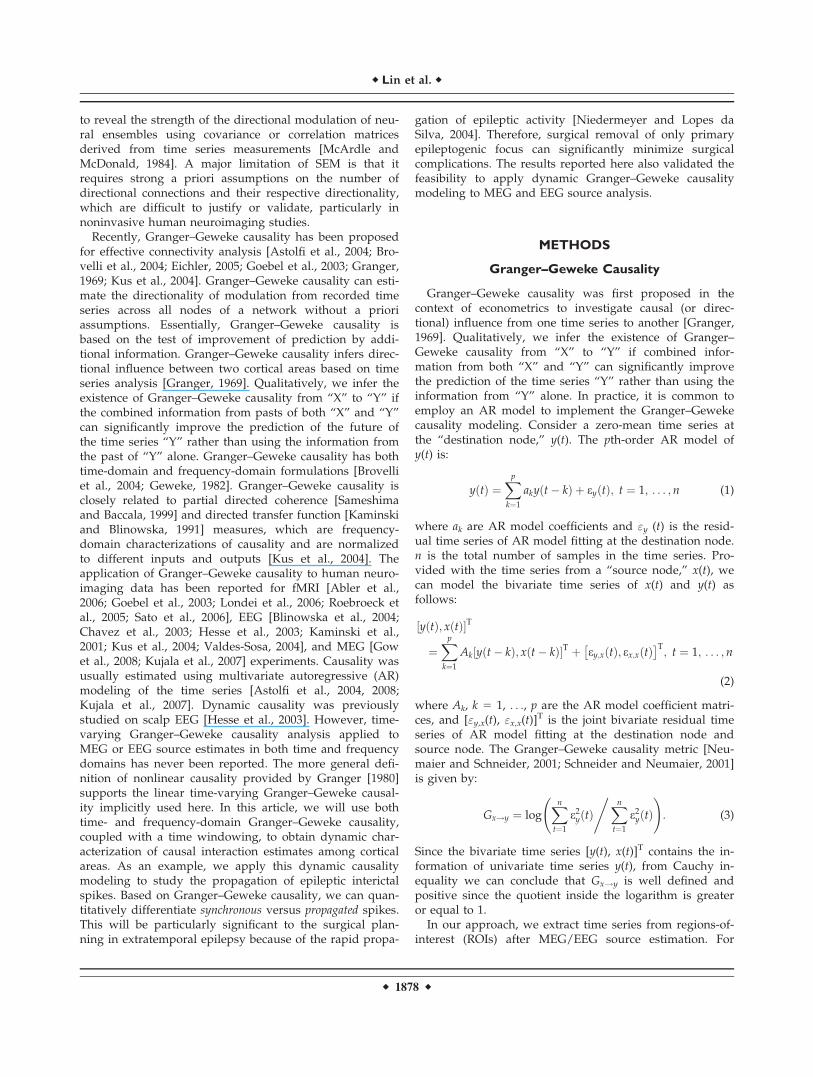
Granger–Geweke causality was first proposed in thecontext of econometrics to investigate causal (or direc-tional) influence from one time series to another [Granger,1969]. Qualitatively, we infer the existence of Granger–Geweke causality from ‘‘X’’ to ‘‘Y’’ if combined infor-mation from both ‘‘X’’ and ‘‘Y’’ can significantly improvethe prediction of the time series ‘‘Y’’ rather than using theinformation from ‘‘Y’’ alone. In practice, it is common toemploy an AR model to implement the Granger–Gewekecausality modeling. Consider a zero-mean time series atthe ‘‘destination node,’’ y(t). The pth-order AR model ofy(t) is:

yðtÞ ¼Xpk¼1

akyðt� kÞ þ eyðtÞ; t ¼ 1; : : : ;n (1)

where ak are AR model coefficients and "y (t) is the resid-ual time series of AR model fitting at the destination node.n is the total number of samples in the time series. Pro-vided with the time series from a ‘‘source node,’’ x(t), wecan model the bivariate time series of x(t) and y(t) asfollows:

yðtÞ; xðtÞ½ �T

¼Xpk¼1

Ak yðt� kÞ; xðt� kÞ½ �T þ ey;xðtÞ; ex;xðtÞ� �T

; t ¼ 1; : : : ; n

(2)

where Ak, k 5 1, . . ., p are the AR model coefficient matri-ces, and ["y,x(t), "x,x(t)]

T is the joint bivariate residual timeseries of AR model fitting at the destination node andsource node. The Granger–Geweke causality metric [Neu-maier and Schneider, 2001; Schneider and Neumaier, 2001]is given by:

Gx!y ¼ logXnt¼1

e2yðtÞ,Xn

t¼1

e2yðtÞ !

: (3)

Since the bivariate time series [y(t), x(t)]T contains the in-formation of univariate time series y(t), from Cauchy in-equality we can conclude that Gx!y is well defined andpositive since the quotient inside the logarithm is greateror equal to 1.

In our approach, we extract time series from regions-of-interest (ROIs) after MEG/EEG source estimation. For

r Lin et al. r

r 1878 r

each pair of time series from two ROIs (‘‘X’’ and ‘‘Y’’), werespectively calculate the Granger–Geweke causality Gx!y

and Gy!x. We will use the SURE criterion (see below) toestimate the order of the AR model and stepwise leastsquares to estimate model parameters [Brovelli et al., 2004;Geweke, 1982]. Let

Fx!y ¼ n� 2p

pexpðGx!yÞ � 1� �

: (4)

Under the null hypothesis, Fx!y asymptotically follows theF-distribution with (p) and (n 2 2p) degrees of freedom,where n denotes the length of the time series andp denotes the order of AR Model [Gourevitch et al., 2006].

Granger–Geweke causality has the frequency-domainrepresentation [Brovelli et al., 2004; Geweke, 1982]:

Gx!yðf Þ ¼ � ln 1� ðRxx � R2xy=RyyÞ Hyxðf Þ

�� ��2Syyðf Þ

!(5)

where x and y subscripts denotes the entries in the matrix.S(f) is the spectral matrix

Sðf Þ ¼ Hðf ÞRHHðf Þ (6)

and H(f) is the transfer function of the system

Hðf Þ ¼Xpk¼0

Ak expðj2pkf Þ !�1

(7)

Ak is the coefficient matrix, andP

is the noise covariancematrix of ["y,x(t), "x,x(t)]

T in the AR model.The statistical inference of frequency-domain Granger–

Geweke causality can be derived with the help of statistic.

Fx!yðf Þ ¼ n� 2p

pexpðGx!yðf ÞÞ� �

(8)

which is analogous to Eq. (4). Under the null hypothesisof no causal relationship from X to Y, Fx!y (f) asympto-tically follows the F distribution with degrees of freedom(p, n 2 2p) [Brovelli et al., 2004; Gourevitch et al., 2006].

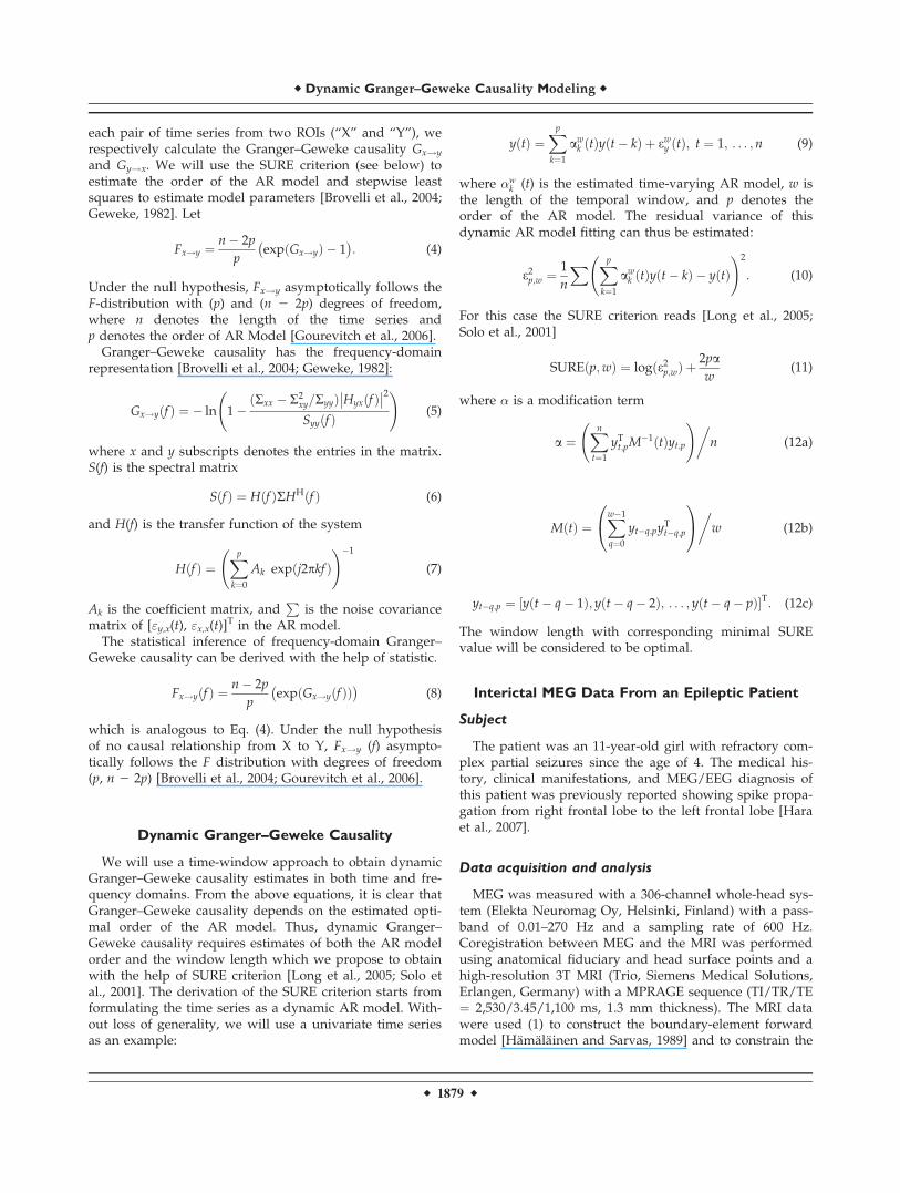
Dynamic Granger–Geweke Causality

We will use a time-window approach to obtain dynamicGranger–Geweke causality estimates in both time and fre-quency domains. From the above equations, it is clear thatGranger–Geweke causality depends on the estimated opti-mal order of the AR model. Thus, dynamic Granger–Geweke causality requires estimates of both the AR modelorder and the window length which we propose to obtainwith the help of SURE criterion [Long et al., 2005; Solo etal., 2001]. The derivation of the SURE criterion starts fromformulating the time series as a dynamic AR model. With-out loss of generality, we will use a univariate time seriesas an example:

yðtÞ ¼Xpk¼1

awk ðtÞyðt� kÞ þ ewy ðtÞ; t ¼ 1; : : : ;n (9)

where �wk (t) is the estimated time-varying AR model, w is

the length of the temporal window, and p denotes theorder of the AR model. The residual variance of thisdynamic AR model fitting can thus be estimated:

e2p;w ¼ 1

n

X Xpk¼1

awk ðtÞyðt� kÞ � yðtÞ !2

: (10)

For this case the SURE criterion reads [Long et al., 2005;Solo et al., 2001]

SUREðp;wÞ ¼ logðe2p;wÞ þ2paw

(11)

where � is a modification term

a ¼Xnt¼1

yTt;pM�1ðtÞyt;p

!�n (12a)

MðtÞ ¼Xw�1

q¼0

yt�q;pyTt�q;p

0@

1A�w (12b)

yt�q;p ¼ yðt� q� 1Þ; yðt� q� 2Þ; : : : ; yðt� q� pÞ½ �T: (12c)

The window length with corresponding minimal SUREvalue will be considered to be optimal.

Interictal MEG Data From an Epileptic Patient

Subject

The patient was an 11-year-old girl with refractory com-plex partial seizures since the age of 4. The medical his-tory, clinical manifestations, and MEG/EEG diagnosis ofthis patient was previously reported showing spike propa-gation from right frontal lobe to the left frontal lobe [Haraet al., 2007].

Data acquisition and analysis

MEG was measured with a 306-channel whole-head sys-tem (Elekta Neuromag Oy, Helsinki, Finland) with a pass-band of 0.01–270 Hz and a sampling rate of 600 Hz.Coregistration between MEG and the MRI was performedusing anatomical fiduciary and head surface points and ahigh-resolution 3T MRI (Trio, Siemens Medical Solutions,Erlangen, Germany) with a MPRAGE sequence (TI/TR/TE¼ 2,530/3.45/1,100 ms, 1.3 mm thickness). The MRI datawere used (1) to construct the boundary-element forwardmodel [Hamalainen and Sarvas, 1989] and to constrain the

r Dynamic Granger–Geweke Causality Modeling r

r 1879 r

source locations to the cortex the subsequent MEG sourceanalysis and (2) for visualizing MEG source analysisresults on inflated cortical surfaces [Dale, 1999; Fischl etal., 1999].

A total of 24 spikes (seven right frontal spikes and 17left frontal spikes) were recorded and separated into leftand right frontal spikes. Seventeen of them are left frontalspikes and seven of them are right frontal spikes. Only 3out of 7 recorded right frontal spikes showed clear propa-gation to the left frontal lobe with a 15–30 ms peak-to-peak latency [Hara et al., 2007]. Epileptic spikes withineach frontal lobe were then temporally aligned and aver-aged. We chose the peak time of the left averaged spikeas 0 ms and the same time origin was applied to theright averaged spike. The source analysis of averaged leftspike (from 17 raw spikes) was done separately by calculat-ing the dynamic statistical parametric mapping (dSPM)[Dale et al., 2000], which is a noise-normalized minimum ‘2-norm source estimate localizing statistically significant neu-ronal activity. Based on our clinical experience and compari-son with the equivalent current dipole (ECD) modelingresults, a critical threshold of 10�6 (uncorrected) was chosenon the dSPM to define the ROIs and to localize the epilepticactivity. Time courses were extracted from all sources withinthe left and right frontal lobe ROIs, respectively. We also cal-culated the time–frequency representation of the timecourses using the continuous wavelet transform (Morletwavelet) to reveal the distribution of the energy in the time–frequency plane [Lin et al., 2004].

To simultaneously estimate the optimal temporal win-dow length and the order of the AR model, we calculatedthe SURE values with the AR model orders varyingbetween 1 and 7 using the ARFIT algorithm [Schneiderand Neumaier, 2001] and the window length varyingbetween 60 and 150 ms. The SURE values for the timecourse averaged across sources locations within the leftand the right frontal lobes were calculated separately. Wechose the window length and the order of the AR modelfor dynamic time-domain and frequency-domain Granger–Geweke causality by choosing those giving the minimalSURE value in the left and right frontal lobe time series.

As discussed earlier, the SURE value was first calculatedusing the average time course within each ROI. Subse-quently, dynamic time-domain Granger–Geweke causalitywas calculated between all left frontal lobe/right frontallobe source pairs using the same the optimal windowlength (w) and AR model order (p) suggested by the SUREcriterion. Using all pairwise causality data, we estimatedthe average and standard deviation of the Granger–Geweke causality. Similarly, using all pairwise time seriesfrom both ROIs, dynamic frequency-domain Granger–Geweke causality between 5 and 40 Hz was also calculatedto give the average and the standard deviation in eachspectrotemporal grid. This frequency range was selectedbased on the time-frequency representation of the timecourses as well as previous studies of cortical oscillatoryinteractions in beta and gamma frequency bands [Kopell

et al., 2000]. We only show statistically significantGranger–Geweke causality with P value of 1% or less.

RESULTS

Spike loci at the left and right frontal lobes localized bythe dSPM are shown in Figure 1A. With respect to thepeak time of the left frontal lobe spike (designated by 0ms), right frontal lobe showed statistically significant activ-ity 21 ms before the peak time of the left frontal lobe. Thetime courses of the left and right frontal lobes within theROI defined by uncorrected P value less than 10�6 wereshown in Figure 1A. Clear separation of the two peaksbetween left and right frontal lobes was observed. Thelocalization results and the spike propagation diagnosiswere further confirmed by a trained epileptologist [Haraet al., 2007]. Two minor activation loci were found in theinferior frontal lobe. These regions are likely artifacts inthe source modeling since they are spatially adjacent toeach other in the convoluted anatomical space and there-fore their MEG lead field is similar. We only included onemajor source ROI in the left and right frontal lobes, respec-tively, to extract time courses for the subsequent causalitymodeling since they matched to the ECD fitting in ourprevious report [Hara et al., 2007]. The average time–fre-quency representation of the time courses in the right andleft frontal ROIs are shown in Figure 1B. Time courses inboth ROIs have energy confined to the time range �50 to50 ms and to frequencies below 20 Hz.

The SURE values for averaged left and right frontallobes is shown in Figure 2. For the left frontal lobe time se-ries, SURE suggested a temporal window of 70 ms and theAR model order of 4. For the right frontal lobe time series,SURE suggested a temporal window of 110 ms and theAR model order of 6. It is rare to obtain one AR model tooptimally model the joint time series in both ROIs as wellas the time series in an individual ROI. We chose the tem-poral window of 70 ms and the AR model order of 4 forthe subsequent Granger–Geweke causality calculationbecause (1) the cost function value is smaller in the leftfrontal lobe calculation than the right frontal lobe calcula-tion, and (2) we desired a more dynamic (a shorter timewindow) and a more simple (a lower AR model order)model.

The time-domain Granger–Geweke causality estimatesare shown in Figure 3 (top panel). The averaged Granger–Geweke causality between the left frontal to right frontallobe and the right frontal to left frontal lobe was difficultto discern before 30 ms of the peak time of Granger–Geweke causality. However, a clear dissociation (P value< 0.01) between these two directional influences was cal-culated at the peak time of the left frontal lobe spike(0 ms) and it continued for 50 ms. The effect durationlikely reflects the chosen temporal window of 70 ms. Wealso calculated the time-domain Granger–Geweke causalityusing the AR model order of 6 and window length of

r Lin et al. r

r 1880 r

110 ms, the optimal values for the right frontal ROI (Fig. 3,bottom panel). The result of unidirectional causal influencefrom the right frontal lobe to the left frontal lobe is consist-ent with that calculated with AR model order of 4 andwindow length of 70 ms.

The top panel of Figure 4 shows the dynamic frequency-domain Granger–Geweke causality with values higherthan 1.5 (P value < 10�4). Between 4 and 22 Hz, from

�150 to 200 ms, there was no statistically significantGranger–Geweke causality found from the left frontal lobeto the right frontal lobe. However, we found statisticallysignificant Granger–Geweke causality spectrally concen-trated between 4 and 20 Hz and temporally concentratedbetween �10 and 0 ms. The frequency-domain Granger–Geweke causality matched the time-domain Granger–Geweke causality showing the right frontal lobe to the left

Figure 1.

(A) Inset: The epileptic activity estimated by dSPM of the aver-

age spike at left and right frontal lobe, respectively. The results

were rendered on the inflated cortical surface where dark gray

and light gray colors indicated sulci and gyri, respectively. The

time origin was chosen such that the peak of the left frontal

lobe spike was 0 ms. Panel: The average and standard deviation

of the time courses at the left and right frontal lobe ROIs.

(B) The average absolute values of the time–frequency represen-

tation of the time courses in the left and right frontal lobes. The

color range was selected to show the range between the 20%

and 80% of the maximal value.

r Dynamic Granger–Geweke Causality Modeling r

r 1881 r

frontal lobe spike propagation. Using a longer time win-dow (110 ms) and a larger AR model order (6), we foundthat consistent unidirectional causality was found from theright frontal lobe to the left frontal lobe (Fig. 4, bottompanel). Compared with the results of 70 ms windowlength and AR model order of 4, higher values in thecausality estimates and wider causal interaction in timewere likely attributed to the more complicated model(higher order in AR modeling) and a longer time window.Note that the time-frequency range showing strong causalinteraction also overlaps with strong energy in the time–frequency representation of the time courses shown inFigure 1B.

DISCUSSION

This study proposes a novel algorithm to estimatedynamic Granger–Geweke causality in both time and fre-quency domains. Based on clinical diagnosis, we testedand validated the feasibility of this approach by comput-ing Granger–Geweke causality estimates from MEG dataacquired from an epileptic patient. Epilepsy can be consid-ered as a disorder of spontaneous neuronal activity. Ingeneral, we expect that the proposed method can beapplied not only to spontaneous activity, but also task-related evoked or induced responses, since the algorithmderives the estimates from time series. The impact ofGranger–Geweke causality estimates in the clinical diagno-sis of spike propagation is that, taken together with other

clinical considerations, such quantitative estimates maysuggest minimal resection applied to the primary epilepto-genic locus only in order to minimize the surgical compli-cations. The causal relationship is already apparent in thesource waveforms. In fact, this clinical case can be consid-ered to ‘‘validate’’ the procedure of calculating dynamicGranger–Geweke causality. Since our calculation is consist-ent with this rather simple clinical case, we are more confi-dent in applying this computational technique in otherrather complicated studies, where noninvasive validationmay be challenging.

This computational tool can be also useful in basic neuro-science studies to elucidate the directional interaction ofbrain areas during behavior, tasks, and cognition. Oscilla-tions are a cardinal signature of brain activity across a broadrange of spatial and temporal scales, ranging from the cellu-lar to the systems level [Berger, 1929; Cohen, 1968; Singer,1999]. Intuitively, oscillations are most effectively character-ized in the frequency domain. Nevertheless, the nonstation-ary nature of oscillatory neural activity suggests that aneffective analysis should span both spectral and temporaldomains. In addition, the brain imaging methods used toinvestigate highly dynamic neural interactions must allowboth high spatial and temporal specificity and sensitivity[Mesulam, 1990]. Coupled with multimodal brain imagingusing high temporal resolution MEG and high spatial reso-lution MRI, a dynamic causality analysis of neural oscilla-tory activity across spatial, temporal, and spectral domainswill provide the opportunity to better understand complexneural information transfer mechanisms.

Figure 2.

The SURE numbers calculated by the left and right frontal lobe time series. Note that the color

codes for the negative SURE values. Therefore, the highest values in each panel of the figure cor-

respond to the minimal values in the cost function, which were indicated by a white star inside a

box with light blue boundary.

r Lin et al. r

r 1882 r

It is possible that the proposed pairwise interactionmodels of pooled ROI time courses may miss some of thefiner interactions or even has the potential problem of falsecausal estimates [Kus et al., 2004]. This is the consequenceof providing partial information of the system: causalinteractions via regions outside the ROI pair wereneglected. In our case, we do not suffer from this issuebecause the data can be accounted for by activity in onlytwo ROIs (in left and right frontal lobes). To apply themethod to a system with multiple ROIs, we can calculateconditional causality [Chen et al., 2006] by including allother ROI time series outside the chosen ROI pairs inorder to avoid the problem of detecting false causal inter-actions or common driving source. This will change thecalculation from pairwise bivariate AR modeling to multi-variate AR modeling. The other challenge to our method

is the situation of missing driving ROIs in the analysis.For example, it is possible to have one common hiddennode driving other ROIs. In this case, our approach willgive false causality estimates among ROIs.

In this study, we used the minimum-norm estimates(MNEs) to extract time courses for the brain space causal-ity modeling. However, because of the cross-talk presentin MNE, the time courses within a cortical region may becorrelated. Because of the nature of correlated informationinside the ROI, we may improve the computational effi-ciency by reducing the dimension of the data. For exam-ple, we may average the time courses within one ROI oruse singular value decomposition to first decompose themultivariate spatiotemporal data and then to removethe last few insignificant components in order to reducethe amount of computation in pairwise causality

Figure 3.

The time-domain dynamic Granger–

Geweke causality. The mean value and

the standard deviation of the

Granger–Geweke causality in both

directions estimated from all pairwise

calculation within ROIs and between

�150 and 200 ms. Top: AR model

order ¼ 4 and window length ¼ 70

ms (optimal for the left frontal lobe in

SURE criterion); bottom: AR model

order ¼ 6 and window length ¼ 110

ms (optimal for the right frontal lobe

in SURE criterion).

r Dynamic Granger–Geweke Causality Modeling r

r 1883 r

calculation. However, the spatiotemporal information maybe incomplete if averaging or a dimension reductionmethod is used. We acknowledge that pairwise calculationbased on partially correlated time courses may be biased.However, this method can empirically estimate the fluctua-tion range of the Granger–Geweke causality. To utilize thistool in planning of clinical treatment, we have to consideralso the precision of source localization in order to extractaccurate time series for the subsequent causality modeling.The spatial accuracy of the MNE source modeling on theMEG data has been studied extensively. Based on our clini-cal experience and comparison with the ECD modeling

results we chose our ROI by selecting a critical threshold ofP value at 10�6 [Hara et al., 2007]. The selection of thethreshold may affect the size of ROI, and subsequently theavailable time courses within a ROI will be different.

The calculated SURE values appeared varying within asmall range over the parametric space (see Fig. 2). How-ever, these numbers themselves do not carry any physicalunit, and they are only used for comparing different mod-els. In this study, we did not study the variability of theSURE values. We only use them to determine the optimalparameters for causality calculation. In fact, using two dif-ferent combinations of the parameters gives consistent

Figure 4.

The frequency-domain dynamic Granger–Geweke causality with spectral analysis between 4 and

22 Hz, and from �150 to 200 ms. Top: AR model order ¼ 4 and window length ¼ 70 ms (opti-

mal for the left frontal lobe in SURE criterion); bottom: AR model order ¼ 6 and window length

¼ 110 ms (optimal for the right frontal lobe in SURE criterion).

r Lin et al. r

r 1884 r

causality results (Figures 3 and 4). This supports that thestability of the SURE criterion.

The SURE values used for determining the optimal tem-poral window length may show no clear minimumbecause the biological mechanism generating the time se-ries measurement does not follow an AR model. It is alsopossible that some window length is deemed optimalbased on prior information. In such cases, it is possible touse a specific window length for dynamic Granger–Geweke causality analyses. It has been reported that thediscrete time filter implementing the windowing domi-nates the frequency resolution of the covariance matrix[Oppenheim et al., 1999]. Additionally, given a fixedamount of temporal observations, the trade-off betweenthe length of a data segment and the number of the seg-ments is essential for the bias and the variance in spectralestimation [Oppenheim et al., 1999]. A Kaiser window[Kuo and Kaiser, 1966] may be used to tune the necessaryfrequency resolution. The selection of temporal segmentscan be proceeded using the ‘‘1/2 overlap’’ principle, whichestimates the instantaneous covariance from data length lby overlapping l/2 samples from previous segments. Thedecision of the segment length l will depend on the sizeand the quality of the collected data.

SEM has been widely used for effective connectivityanalysis to elucidate directional causal interaction amongbrain areas. One principal difference between SEM andGranger–Geweke causality is that SEM is a more model-driven approach, i.e., a prior directional connectivitymodel must be provided before parameter estimation,while Granger–Geweke causality is a more data-drivenapproach where directional modulation is directly esti-mated from the time series without any prior information.However, AR modeling is still used in the calculation. Onelimitation of Granger–Geweke causality is the temporal re-solution. Even using a temporal windowing approach asreported here, Granger–Geweke causality cannot resolvecausal modulation within the chosen temporal window.SEM, on the other hand, is capable of achieving the high-est temporal resolution by time-point–by–time-point calcu-lation. Theoretically it is possible to combine Granger–Geweke causality and SEM in order to avoid the heuristicspecification of the directional connectivity while achievingthe highest temporal resolution possible. Specifically,Granger–Geweke causality can be utilized to estimate stat-istically significant directional paths for each possible pairof sources, to construct a directional connectivity matrix inSEM. Together with dynamic covariance matrix estimatedfrom the data, we may dynamically estimate path coeffi-cients at the millisecond temporal resolution.

CONCLUSIONS

We employed dynamic Granger–Geweke causality esti-mates in both time and frequency domain in order toinvestigate directional influence among brain areas. This

approach was applied to clinical spike propagation case toquantitatively ascertain the epileptic event propagatingfrom the right frontal lobe to the left frontal lobe. Weexpect that the same algorithm can be applied to MEG,EEG, fMRI, or combined modality data in order to helpbetter understand the complex interactions within thehuman brain.

REFERENCES

Abler B, Roebroeck A, Goebel R, Hose A, Schonfeldt-Lecuona C,Hole G, Walter H (2006): Investigating directed influencesbetween activated brain areas in a motor-response task usingfMRI. Magn Reson Imaging 24:181–185.

Astolfi L, Cincotti F, Mattia D, Salinari S, Babiloni C, Basilisco A,Rossini PM, Ding L, Ni Y, He B, Marciani MG, Babiloni F(2004): Estimation of the effective and functional human corti-cal connectivity with structural equation modeling anddirected transfer function applied to high-resolution EEG.Magn Reson Imaging 22:1457–1470.

Astolfi L, Cincotti F, Mattia D, De Vico Fallani F, Tocci A, Colo-simo A, Salinari S, Marciani MG, Hesse W, Witte H, Ursino M,Zavaglia M, Babiloni F (2008): Tracking the time-varying corti-cal connectivity patterns by adaptive multivariate estimators.IEEE Trans Biomed Eng 55:902–913.

Berger H (1929): Ueber das Elektrenkephalogramm des Menschen.Archiv fuer Psychiatrie und Nervenkrankheiten 87:527–570.

Blinowska KJ, Kus R, Kaminski M (2004): Granger causality andinformation flow in multivariate processes. Phys Rev E StatNonlinear Soft Matter Phys 70(5, Part 1):050902.

Brovelli A, Ding M, Ledberg A, Chen Y, Nakamura R, Bressler SL(2004): Beta oscillations in a large-scale sensorimotor corticalnetwork: Directional influences revealed by Granger causality.Proc Natl Acad Sci USA 101:9849–9854.

Chavez M, Martinerie J, Le Van Quyen M (2003): Statistical assess-ment of nonlinear causality: Application to epileptic EEG sig-nals. J Neurosci Methods 124:113–128.

Chen Y, Bressler SL, Ding M (2006): Frequency decomposition ofconditional Granger causality and application to multivariateneural field potential data. J Neurosci Methods 150:228–237.

Cohen D (1968): Magnetoencephalography: Evidence of magneticfields produced by alpha-rhythm currents. Science 161:784–786.

Dale AM (1999): Optimal experimental design for event-relatedfMRI. Hum Brain Mapp 8:109–114.

Dale AM, Liu AK, Fischl BR, Buckner RL, Belliveau JW, LewineJD, Halgren E (2000): Dynamic statistical parametric mapping:combining fMRI and MEG for high-resolution imaging of corti-cal activity. Neuron 26:55–67.

Eichler M (2005): A graphical approach for evaluating effectiveconnectivity in neural systems. Philos Trans R Soc Lond B BiolSci 360:953–967.

Fischl B, Sereno MI, Dale AM (1999): Cortical surface-based analy-sis. II. Inflation, flattening, and a surface-based coordinate sys-tem. Neuroimage 9:195–207.

Geweke J (1982): Measures of conditional linear dependence andfeedback between time series. J Am Stat Assoc 77:304–313.

Goebel R, Roebroeck A, Kim DS, Formisano E (2003): Investigat-ing directed cortical interactions in time-resolved fMRI datausing vector autoregressive modeling and Granger causalitymapping. Magn Reson Imaging 21:1251–1261.

r Dynamic Granger–Geweke Causality Modeling r

r 1885 r

Gourevitch B, Bouquin-Jeannes RL, Faucon G (2006): Linear andnonlinear causality between signals: methods, examples andneurophysiological applications. Biol Cybern 95:349–369.

Gow DW Jr, Segawa JA, Ahlfors SP, Lin FH (2008): Lexical influ-ences on speech perception: A Granger causality analysis ofMEG and EEG source estimates. Neuroimage 43:614–623.

Granger CWJ (1969): Investigating causal relations by econometricmodels and cross-spectral methods. Econometrica 37:424–438.

Granger CWJ (1980): Testing for causality. J Econ Dyn Control 2:329–352.

Hamalainen MS, Sarvas J (1989): Realistic conductivity geometrymodel of the human head for interpretation of neuromagneticdata. IEEE Trans Biomed Eng 36:165–171.

Hara K, Lin FH, Camposano S, Foxe DM, Grant PE, Bourgeois BF,Ahlfors SP, Stufflebeam SM (2007): Magnetoencephalographicmapping of interictal spike propagation: A technical and clini-cal report. AJNR Am J Neuroradiol 28:1486–1488.

Hesse W, Moller E, Arnold M, Schack B (2003): The use of time-variant EEG Granger causality for inspecting directed interde-pendencies of neural assemblies. J Neurosci Methods 124:27–44.

Kaminski M, Ding M, Truccolo WA, Bressler SL (2001): Evaluatingcausal relations in neural systems: Granger causality, directedtransfer function and statistical assessment of significance. BiolCybern 85:145–157.

Kaminski MJ, Blinowska KJ (1991): A new method of the descrip-tion of the information flow in the brain structures. BiolCybern 65:203–210.

Kopell N, Ermentrout GB, Whittington MA, Traub RD (2000):Gamma rhythms and beta rhythms have different synchroniza-tion properties. Proc Natl Acad Sci USA 97:1867–1872.

Kujala J, Pammer K, Cornelissen P, Roebroeck A, Formisano E,Salmelin R (2007): Phase coupling in a cerebro-cerebellarnetwork at 8–13 Hz during reading. Cereb Cortex 17:1476–1485.

Kuo FF, Kaiser JF (1966): System Analysis by Digital Computer,Vol. XIV. New York: Wiley. 438 p.

Kus R, Kaminski M, Blinowska KJ (2004): Determination of EEGactivity propagation: Pair-wise versus multichannel estimate.IEEE Trans Biomed Eng 51:1501–1510.

Lachaux JP, Rodriguez E, Martinerie J, Varela FJ (1999): Mea-suring phase synchrony in brain signals. Hum Brain Mapp 8:194–208.

Lin FH, Witzel T, Hamalainen MS, Dale AM, Belliveau JW, Stuf-flebeam SM (2004): Spectral spatiotemporal imaging of cortical

oscillations and interactions in the human brain. Neuroimage23:582–595.

Londei A, D’Ausilio A, Basso D, Belardinelli MO (2006): A newmethod for detecting causality in fMRI data of cognitive proc-essing. Cogn Process 7:42–52.

Long CJ, Brown EN, Triantafyllou C, Aharon I, Wald LL, Solo V(2005): Nonstationary noise estimation in functional MRI.Neuroimage 28:890–903.

McArdle JJ, McDonald RP (1984): Some algebraic properties of thereticular action model for moment structures. Br J Math StatPsychol 37 (Part 2):234–251.

Mesulam M-M (1990): Large-scale neurocognitive networks anddistributed processing for attention, language, and memory.Ann Neurol 28:597–613.

Neumaier A, Schneider T (2001): Estimation of parameters andeigenmodes of multivariate autoregressive models. ACM TransMath Softw 27:27–57.

Niedermeyer E, Lopes da Silva FH (2004): Electroencephalogra-phy: Basic Principles, Clinical Applications, and Related Fields.Philadelphia: Lippincott Williams & Wilkins.

Oppenheim AV, Schafer RW, Buck JR (1999): Discrete-Time SignalProcessing, Vol. XXVI. Upper Saddle River, NJ: Prentice Hall.870 p.

Roebroeck A, Formisano E, Goebel R (2005): Mapping directedinfluence over the brain using Granger causality and fMRI.Neuroimage 25:230–242.

Sameshima K, Baccala LA (1999): Using partial directed coherenceto describe neuronal ensemble interactions. J Neurosci Meth-ods 94:93–103.

Sato JR, Junior EA, Takahashi DY, de Maria Felix M, BrammerMJ, Morettin PA (2006): A method to produce evolving func-tional connectivity maps during the course of an fMRI experi-ment using wavelet-based time-varying Granger causality.Neuroimage 31:187–196.

Schneider T, Neumaier A (2001): Algorithm 808: ARfit—A Matlabpackage for the estimation of parameters and eigenmodes ofmultivariate autoregressive models. ACM Trans Math Softw27:58–65.

Singer W (1999): Neuronal synchrony: A versatile code for thedefinition of relations? Neuron 24:49–65, 111–125.

Solo V, Purdon P, Weisskoff R, Brown E (2001): A signal estimationapproach to functional MRI. IEEE Trans Med Imaging 20:26–35.

Valdes-Sosa PA (2004): Spatio-temporal autoregressive modelsdefined over brain manifolds. Neuroinformatics 2:239–250.

r Lin et al. r

r 1886 r