A Dynamic-Bayesian Network Framework for Modeling

and Evaluating Learning from Observation

Santiago Ontanona,, Jose L. Montanab, Avelino J. Gonzalezc

aDrexel University, Philadelphia, PA, USAbUniversity of Cantabria, Santander, Spain

cUniversity of Central Florida, Orlando, FL, USA

Abstract

Learning from Observation (LfO), also known as Learning from Demon-stration, studies how computers can learn to perform complex tasks by ob-serving and thereafter imitating the performance of a human actor. Althoughthere has been a significant amount of research in this area, there is no agree-ment on a unified terminology or evaluation procedure. We outline a possibletheoretical framework for the quantitative modeling and evaluation of LfOtasks. We note that: (1) the information captured through the observa-tion of agent behaviors does not occur as a sample of a state to action mapbut as the realization of a stochastic process; (2) these observations may besimplified at the price of some loss of model accuracy and abstraction byintroducing dynamic models with hidden states for which the learning andmodel evaluation tasks can be reduced to minimization and estimation ofsome stochastic similarity measures such as crossed entropy. Specifically, themain contributions of this paper are: a unified framework for LfO, whichallows us to provide an easy characterization of the types of behaviors thatcan be learned from observation and makes explicit the relation of LfO withsupervised learning; a framework for LfO problems based on graphical mod-els; and a collection of evaluation metrics for LfO algorithms, which we showto better capture the performance of LfO algorithms than prediction error.

Keywords: Learning from Observation, Dynamic Bayesian Networks

∗Corresponding authorEmail addresses: santi@cs.drexel.edu (Santiago Ontanon), montanjl@unican.es

(Jose L. Montana), gonzalez@ucf.edu (Avelino J. Gonzalez)

Preprint submitted to Expert Systems with Applications December 7, 2013

1. Introduction

Learning by watching others do something is a natural and highly effec-tive way for humans to learn. It is also an intuitive and highly promisingavenue for machine learning. It provides a way for machines to learn howto perform tasks in a more natural fashion. For many tasks, learning fromobservation is more natural than providing static examples that explicitlycontain the solution, as in the traditional supervised learning approach. It isalso easier than manually creating a controller that encodes the desired be-havior. Humans typically just perform the task and trust that the observercan figure out how to successfully imitate the behavior.

Although there has been a significant amount of research in learning fromobservation (LfO), there is no agreement on a unified terminology or evalu-ation procedure. Works reported in the literature also refer to learning fromdemonstration, learning by imitation, programming by demonstration, or ap-prenticeship learning, as largely synonymous to learning from observation.In learning from demonstration, a human purposely demonstrates how toperform a task or an action, expressly to teach a computer agent how toperform the same task or mission. We consider learning from demonstrationto be a specialization of LfO and define the latter as a more general learningapproach, where the actor being observed need not be a willing participant inthe teaching process. This could include opponents being observed in teamgame competition or the enemy tactics being learned through observation(and thereafter modeled).

In this paper, we argue that LfO is fundamentally different from tra-ditional supervised, unsupervised and reinforcement learning approaches.Clearly, LfO differs from unsupervised learning because the examples (demon-strations) contain an implicit indication of correct behavior. Also, LfO clearlydiffers from reinforcement learning because LfO learns from a collection oftraces (or trajectories), rather than from trial and error through a reinforce-ment signal (although, as we will see later, some reinforcement learning ap-proaches use LfO as a way to guide the learning process, e.g. [1]).

LfO can be more readily likened to supervised learning, but two key dif-ferences exist. First, in LfO the learning examples are time-based, continuousand not easily separable through the duration of the exercise. Furthermore,no explicit linkage between cause and effect is provided, but must be ex-tracted automatically by the learning algorithm. The cause of an actionmight very well be something perceived in a past instant of time, rather than

2

in the current perceptual state. Thus, the form of supervised learning thatis more related to LfO is that of sequential learning [2].

A second, key, difference is on what needs to be learned. Supervisedmachine learning techniques (including sequential ones) focus on learningmodels that minimize the prediction error, i.e. they learn to predict the out-put of the learning task given the input, on average. However, that is notthe goal in LfO. Consider an agent trying to learn by observing the behaviorof an actor who, while driving a car, chooses a different random speed eachminute with a mean of 100kph and a certain variance. A standard super-vised learning method would learn to predict that the speed should alwaysbe 100kph (because that is the value that yields minimum prediction error).However, an LfO agent should learn that the speed must be changed whenappropriate with a particular variance. This illustrates that LfO aims atreplicating the behavior of the actor, instead of minimizing the predictionerror. For that reason, supervised learning techniques for LfO have to beemployed with care, and a different class of algorithms is required in the gen-eral case. However, as our previous work shows, some types of learning fromobservation tasks can be addressed with supervised learning (for example, aswe will see later, when learning state-less deterministic behavior, minimizingprediction error is equivalent to replicating behavior).

This paper focuses on a unified framework for learning from observation.We will provide both an intuitive description of the framework, as well as aformal statistical model of LfO, based on the formalism of Dynamic BayesianNetworks (DBN) [3]. The main contributions of this paper, are:

• A formal statistical model of LfO, that includes a taxonomy of thedifferent behaviors that can be learned through LfO.

• An explicit formulation of the difference between supervised learningand LfO algorithms. This is important, since in most LfO work, stan-dard supervised algorithms (like neural networks, or nearest-neighborclassifiers) are used. As stated above, there are many LfO behaviorsfor which those algorithms are not appropriate.

• A proposal for new evaluation metrics. Our framework makes explicitthe reason for which standard metrics, like classification accuracy arenot appropriate for LfO in some situations, and do not properly reflecthow well an LfO algorithms has learned. We will describe the reasons

3

for this, and propose an alternative evaluation approach based on theKullback-Liebler divergence.

The remainder of this paper is organized as follows. Section 2 briefly sum-marizes previous research in the field. After that, Section 3 introduces acommon framework and vocabulary for learning from observation, includingan intuitive description of the different behaviors that can be attempted withLfO, and how performance can be measured. Section 4 presents a statisti-cal formalization of the problem, that leads to the three insights outlinedabove. Section 5 focuses on evaluation metrics for LfO algorithms. Finally,Section 6 presents an empirical validation of two of our claims: a) supervisedlearning algorithms are not appropriate for some LfO behaviors, and b) ourproposed evaluation metric is more accurate than then typical metrics usedin the literature of LfO.

2. Learning from Observation Background

Work in learning from observation can be traced back to the early daysof AI. For instance, Bauer [4] proposed in 1979 to learn programs from ex-ample executions, which basically amounts to learning strategies to performabstract computations by demonstration. This form of learning has beenespecially popular in robotics [5]. Another early mention of learning fromobservation comes from Michalski et al. [6] who define it merely as unsuper-vised learning, or Pomerleau [7], who developed the ALVINN system thattrained neural networks from observation of a road-following automobile inthe real world.

More recent work on the more general LfO subject came from Sammutet al [8], Sidani [9] and Gonzalez et al [10]. Fernlund et al. [11] used learningfrom observation to build agents capable of driving a simulated automobilein a city environment. The neural network approach to learning from obser-vation has remained popular, and contributions are still being made, such asthe work of Moriarty and Gonzalez [12], in the context of computer games.

In robotics, learning from demonstration has been extensively used toimplement human behavior in humanoid robot movements. Bentivegna andAtkeson [13] used learning from demonstration to teach a humanoid robotto play air hockey using a set of action primitives, each describing a certainbasic action. Chernova and Veloso [14, 15] studied the problem of multi-robot learning from demonstration where a group of agents was shown how

4

to collaborate with each other. Other important work was reported by Schaal[16], Atkeson et al. [17] and Argall et al. [18] among many others.

Konik and Laird [19] studied learning from observation with the SOARsystem by using inductive logic programming techniques.

A theoretical approach to LfO is that of Khardon [20], where he proposedto use a systematic algorithm that enumerates all the possible finite-statemachines (given the inputs and outputs of a given domain), and rank themaccording to their probability of achieve the goal, and to how consistent theyare with the behavior observed from the expert. An important differencebetween Khardon’s work and most work on LfO is that Khardon assumedthat the learning agent has access to a description of the goal (i.e. thelearning agent knows, during learning, if a particular behavior would achievethe goal or not in a given scenario). Most work on LfO just assumes thatthe only form of input are samples of behavior from the expert, without anyexplicit description of the goal to be achieved.

Other significant work done under the label of learning from demonstra-tion has emerged recently in the case-based reasoning (CBR) community.Floyd et al. [21] present an approach to learn how to play RoboSoccer byobserving the play of other teams. Ontanon and associates [22, 23, 24] uselearning from demonstration in the context of case-based planning, appliedto real-time strategy games. Rubin and Watson [25] used LfO for creating aPoker-playing agent. And LaMontagne et al. [26] study techniques based onconditional entropy to improve case acquisition in CBR-based LfO. The maindifference between the work based on CBR and the previous work presentedin this section is that CBR methods are related to lazy machine learningtechniques that do not require any form of generalization during learning.In CBR, thus, learning becomes a pure memorization of new cases, and anykind of generalization is delayed until problem solving time.

Additionally, Inverse Reinforcement Learning (IRL) [27] is closely relatedto learning from observation, where the focus is on reconstructing the rewardfunction given optimal behavior (i.e. given a policy, or a set of trajectories).One of the main difficulty in IRL is that there might be different rewardfunctions that correspond to the observed behavior, and heuristics need tobe devised to bias the learning towards the set of reward functions of in-terest. The paradigm of inverse reinforcement learning has recently receivedincreased attention for its applications to LfO [28, 29, 30]. The key differencebetween the IRL approach to LfO and the supervised learning approachesmentioned above is that IRL tries to learn the goal (reward function) of the

5

expert, to then use standard reinforcement learning to learn optimal behav-ior to achieve such goal. The supervised learning approach to LfO, however,aims at learning to directly predict the actions of the expert from the ob-served behavior. These approaches, however, ignore the fact that the expertmight have internal state. For example, IRL assumes the expert is solving aMarkov Decision Process (MDP), and thus has no additional internal stateother than the observed state. For IRL to be applicable to the general prob-lem of LfO, it needs to consider partially observable MDPs (POMDP), toaccount for the lack of observability of the expert’s state.

Finally, the approaches that are most related to the model presented inthis paper, are those based on Markov Decision Processes (MDP). For exam-ple, Dereszynski et al. [31] describe an approach based on Hidden MarkovModels to learn a model of the behavior of agents in real-time strategy games.Pentland and Liu [32] used Hidden Markov Models (HMMs) to infer the in-ternal state of an automobile driver.

An in-depth overview of the area is out of the scope of this paper, theinterested reader is referred to [18] for a recent overview. Moreover, we cansee that while a significant amount of work has been on-going over the last20 years, the problem does not enjoy a modicum of formalization, or even ofagreement in terminology. For example, in the in-depth recent overview byArgall et al. [18], or in the recent formalization by Billing and Hellstrom [33],they present a formalization that only covers learning Markovian processesfrom observation (thus, not covering the whole spectrum of existing LfOtechniques, as we will show later). In this paper, we hope to provide a steptowards this missing formalization.

3. Learning from Observation

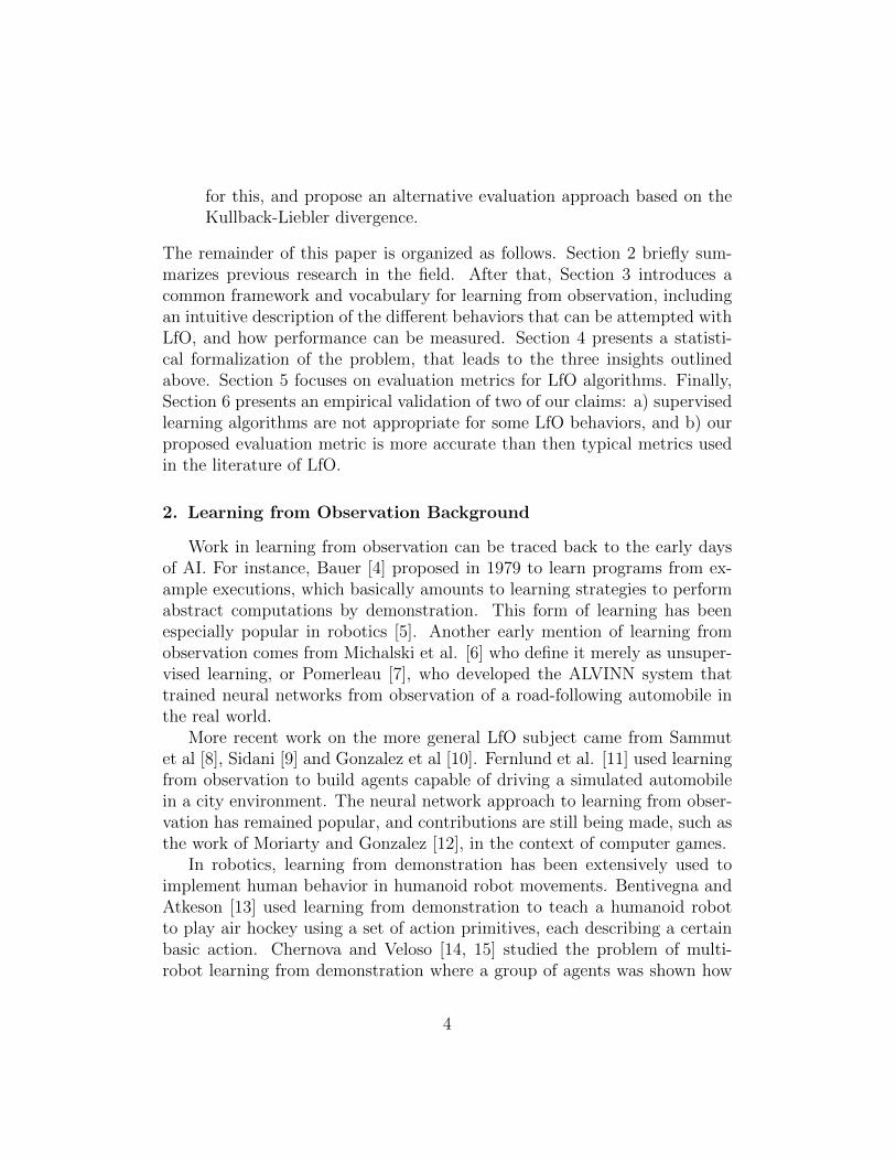
In this section we outline a framework that attempts to be a unification ofprevious work in the area (which will be further formalized in Section 4). Letus start by introducing the different elements appearing in LfO (illustratedin Figure 1):

• There is a task T to be learned, which can be either achieving a con-dition (such as building a tower, or defeating an enemy), maintainingsome process over time (such as keeping a car on the road), or maximiz-ing some value. In general, T can be represented as a reward function,which has to be maximized.

6

actionlearning trace

environment

perception

learning agent

actortask

A

CT

x y

E

[(x1, y1), ..., (xn, yn)]

Figure 1: Elements appearing in learning from observation.

• There is an environment E.

• There is one actor (or trainer, expert, or demonstrator) C, who per-forms the task T in the environment (there can in principle be also bemore than one actor).

• There is a learning agent A, whose goal is to learn how to achieve T inthe environment E by observing C (some work in the literature, suchas [14] or [34] focus on multiagent learning from observation, in thispaper, we will focus on single-agent LfO).

In learning from observation, the learning agent A first observes one orseveral actors performing the task to be learned in the environment, andrecords their behavior in the form of traces. Then, those traces are usedto learn how to perform T . The environment in which the learning agentobserves the actor perform the task and the one in which the agent later needsto perform do not necessarily have to be exactly the same. For instance, inthe context of a computer game, the learning agent might observe the actorplay the game in a particular map, and then try to perform in a differentmap. Moreover, we are assuming that the agent does not have access to adescription of T , and thus, behavior must be learned purely by observationand imitation of the behavior of the expert.

Let BC be the behavior of an actor C. By behavior, we mean the controlmechanism, policy, or algorithm that an actor or a learning agent uses todetermine which actions to execute over time. In subsequent sections we will

7

provide a more formal definition of behavior, based on the notion of stochasticprocesses, but this intuitive idea suffices for the purpose of this section.

In a particular execution, a behavior BC is manifested as the series ofactions that the actor executes over time, which we call a behavior trace, orBT . Depending on the type of the task to be learned, the actions of theactor can vary in nature. These could be atomic actions, durative actions,or just a collection of control variables y that are adjusted over time. Ingeneral, we will assume that the actor can control a collection of variables,and thus, a behavior trace is defined as the variation of these variables overtime: BTC = [y1, ..., yn], where, yt represent the value of the control variablesat time t, which we will call the action executed by the actor at time t.

The most common situation is to assume that the learning agent canexecute the same set of actions as the actor (i.e. that the set of controlvariables of the learning agent is the same as that of the actor). Otherwise,the LfO problem becomes harder, since a mapping between the learning agentactions and the actor’s actions must be learned as well. Moreover, the stateof the environment might not be directly observable. Both the actor andthe learning agent perceive it through a collection of input variables x. Theevolution of the environment, as observed by the actor, is captured into aninput trace: IT = [x1, ..., xn].

The combination of actor behavior plus input trace, constitutes a learningtrace in learning from observation: LT = [(x1, y1), ..., (xn, yn)].

We assume traces are indexed in a finite set, and that sampling at a givenfrequency will be used when learning tasks in environments with continuoustime, e.g. [13].

The task T to perform is defined as a reinforcement signal T (x, y), whichassigns a reinforcement value T (x, y) ∈ R to each state/action pair (x, y).When the learning agent observes the actor, it is assumed that the actor istrying to maximize T . Notice that a reinforcement signal is general enoughto capture tasks such as “reaching a terminal state” (by having a positivereward in that state, and 0 in any other state), “staying in a certain set ofstates”, etc. However, in most work on LfO, only the actor has access to thedefinition of the task T , which is unknown to the learning agent A. We willthus, distinguish the two situations, when A has access to T , and when Adoes not.

1. If the reward function T is available to the learning agent A, LfO canbe defined as:

8

Given: An environment E, perceived through a set of input variablesx, and acted upon by a set of control variables y, a collection oflearning traces LT1, ..., LTk, and a reward function T .

Learn: A behavior B that maximizes T . In this case, the set of inputtraces from the expert, are typically just used to learn an initialbehavior, that is later optimized (e.g. using reinforcement learn-ing) to maximize T . In other words, in this situation, the experttraces are just used to speed up the convergence to a behaviorthat maximizes T . For example, the work of Lin [1] falls underthis category.

2. If T is not available to the learning agent A, LfO can be defined as:

Given: An environment E, perceived through a set of input variablesx, and acted upon by a set of control variables y, and a collectionof learning traces LT1, ..., LTk

Learn: A behavior B that behaves in the same way as the actor doesin the environment E, given the same inputs. For example, thework of Fernlund et al. [11] falls into this category. Given that noreward function T is available in this case, one of the open chal-lenges in the LfO literature, is how to formally define “in the sameway”, i.e. how to define performance metrics for LfO algorithms,which we address below.

Measuring the success of a LfO system is not trivial [18]. In supervisedlearning, a simple way is to leave some training examples out, and use themas test. The equivalent in LfO would be to leave some learning traces out,and use them to verify the learned behavior B. However, in LfO we haveto compare behavior traces, which is not trivial. For example, if at somepoint of time t two traces differ, it might be meaningless to compare therest of the traces, since from that point on, they might completely diverge.Therefore, just counting percentage of actions correctly predicted is not agood approach.

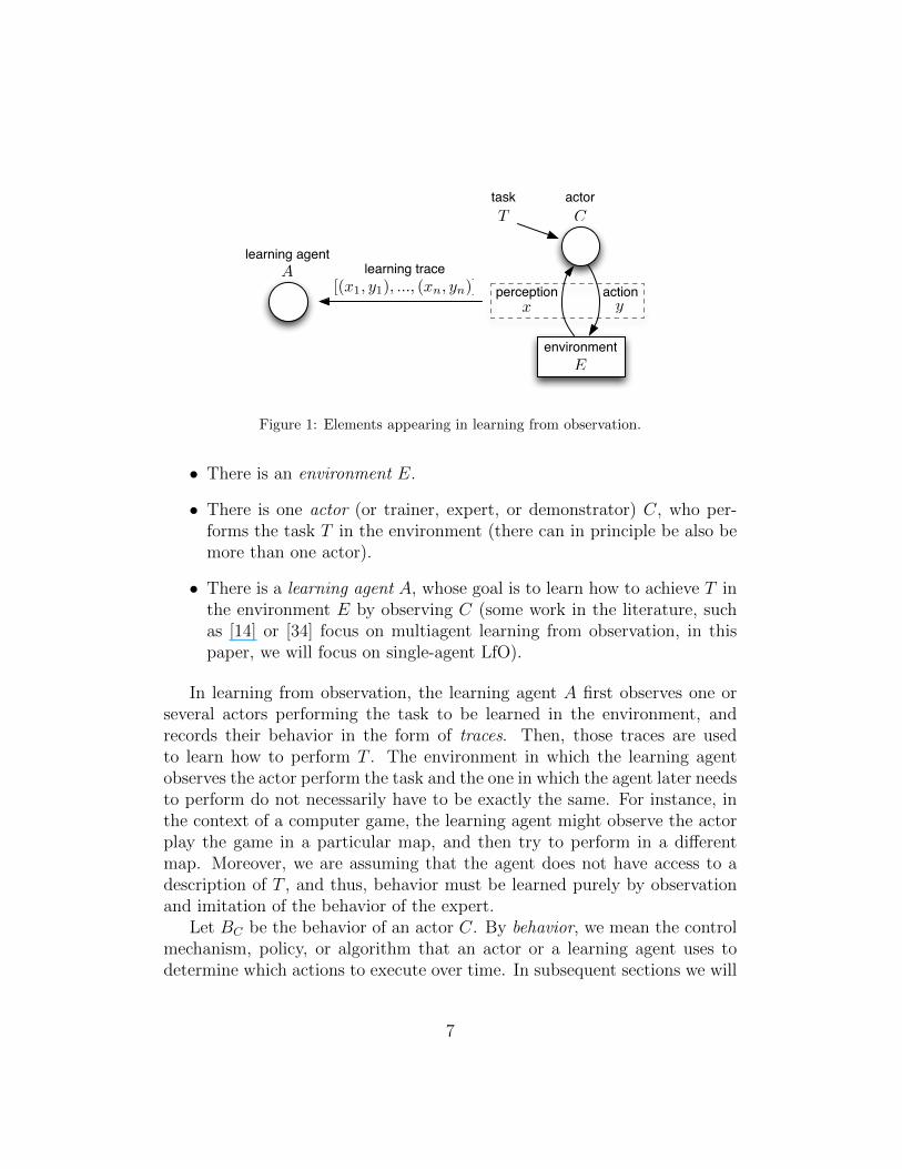
Furthermore, if the behavior to be learned is stochastic, comparing in-dividual actions would not be a good approach. Imagine that an actor isdemonstrating a behavior which consists of picking an action at random fromthe set {−1, 0, 1} at each executing cycle. There are two learning agents, A1

and A2. After observing this actor, the behavior learnt by A1 consists of al-ways executing 0 (which gives the best mean-square error prediction error);

9

the behavior learnt by A2, however, is the correct one (randomly execute oneof the three actions at each cycle). Now, if we were to evaluate the perfor-mance of these two agents using a standard loss function, like mean-squareerror using a leave-one-out method, agent A1 would get an average error ofabout 0.66, and agent A2 would achieve one of about 0.88. However, it wasA2 who properly learnt the behavior of the actor. Therefore, simple measuressuch as classification accuracy or mean-square error are not enough to mea-sure the performance of LfO algorithms and determine whether the learnedbehavior is similar or not to the expert behavior. We need performancemeasures that can compare probability distributions.

Three basic strategies have been explored in the literature to evaluateagents trained through LfO:

• Output Evaluation: This approach compares the actions executed bythe learning agent A against the actions executed by the actor C. Thisevaluation method is the most similar to supervised learning. The setof learning traces can be divided into a training set and a test set, anduse the test set of traces to evaluate the learning agent. One must becareful when using this evaluation method, since, as mentioned earlier,comparing traces in general is not trivial. If we assume the behavior tobe learned is a deterministic observation to action mapping, i.e. thatthe action yt to execute at time t only depends on the input variablesxt (the current state), then the learning traces can be split up intostandard training instances (pairs observation/action) and use standardsupervised learning classification accuracy, for example. For example,this is the approach taken by Floyd et al. [21]. However, this simpleapproach would not work for more complex behaviors (e.g. behaviorsthat cannot be represented as an observation to action mapping).

• Performance Evaluation: This approach measures how well thelearning agent A performs T , regardless of whether it is performingsimilar actions to the actor C or not. This can be measured, for ex-ample, by computing the accumulated or discounted reward obtainedby the learning agent. For example, in a car driving scenario, we couldmeasure whether the learning agent can keep the car in the road. Forexample, the work of Ontanon et al. [23] uses this strategy.

• Model Evaluation: This approach is based on manually comparingthe actual model (program, state machine, set of rules, probability

10

distribution, policy, or any other decision procedure) that the agent haslearned against the model the actor was using to generate the traces.For example, if we know that the actor was following a specific finite-state machine, we can manually see if the learning agent has learnedexactly the same finite-state machine. Early work on programming bydemonstration [4] used this paradigm to evaluate success. However,given that this is not a practical approach to evaluate performance(since it requires manual inspection of the learned behavior), it is notused in practice.

The previous three approaches, intuitively, correspond to: compare theactions (output evaluation), compare the effect of the actions (performanceevaluation), and compare the procedure executed to generate the actions(model evaluation). Model evaluation is typically a manual process, whereasperformance evaluation is directly measurable (it requires testing to whatdegree the task the learning agent was supposed to learn was achieved).However, output evaluation is a more complex matter, for which we willprovide a formalization in Section 5.

This section has presented the basic vocabulary in LfO. The followingsubsection presents a taxonomy of different families of behaviors, discussingwhich LfO algorithms can be used to learn each of them.

3.1. Levels of Learning from Observation

It is intuitively evident that not all LfO learning algorithms will work forlearning all behaviors. Therefore, we next attempt to categorize the typesof behaviors that can be learned through LfO. First we must state that thegeneral type of problems LfO addresses are those that involve learning sometype of control function (i.e. a behavior). Such behaviors may be low level,such as motor skills, or higher level, such as strategic decision making.

Several factors determine the complexity of a behavior to be learnedthrough LfO:

• Are the variables continuous or discrete?

• Is the actor behavior observable? If the learning agent cannot perceivethe same variables (x) of the environment as the actor, or if the learnercannot fully perceive the control variables (y) that the actor moanip-ulates, the learning task becomes very complex. This basically means

11

Generalization? Memory? Level

no no Level 1: Strict Imitation

yes no Level 2: Reactive Behavior

yes yes Level 3: Memory-based Behavior

Table 1: Characterization of the different levels of difficulty of learning from observation.

that the behavior of the actor is not fully observable (input or outputvariables).

• Does the learning task require generalization? Generalization is theprocess by which a general statement is obtained by inference fromspecific instances. Some tasks, as we will show below, do not requiregeneralization.

• Does the learning task require memory? In some tasks, the learningagent has to take into account events that occurred earlier in timein order to take a decision. In such tasks, we say that memory isrequired. This basically translates to whether the behavior to be learntis Markovian or not (i.e. whether the action yt only depends on thecurrent state observation xt or not).

Let us then focus on the last two of those factors, since they define thethree major families of behaviors that can be learned through learning fromobservation (as shown in Table 1):

Level 1 - Strict Imitation: some behaviors do not require feedback fromthe environment, and thus neither generalization nor memory. Thelearned behaviors are a strict function of time. For that reason, itdoes not matter whether the environment is known or unknown. Thelearning algorithms to solve these tasks only require pure memorization.One can think of these behaviors as requiring open-loop control. Robotsin factories are an instance of this type of learning, where the pieces arealways in the exact same place each time the robot performs a learnedaction.

Level 2 - Reactive Behavior: reactive behaviors correspond to input toaction mapping, without requiring memory. Generalization is desirablewhen learning these behaviors. Reactive behaviors are Markovian, since

12

they can be represented as a a mapping from the perceived state of theenvironment to the action, i.e. a policy. Learning how to play somevideo games such as pong and space invaders would fit this category.

Level 3 - Memory-based Behavior: This level includes behaviors in whichthe current state of the world is not enough to determine which actionsto execute, previous states might have to be taken into account. Thebehavior to learnt is not just a situation to action mapping, but mighthave internal state. For example, learning how to play a game likeStratego is a task of Level 3. Stratego is a strategy game similar toChess, but where the players do not see the types of the pieces of theopponent, only their locations. After certain movements, a player cantemporally observe the type of one piece, and must remember this inorder to exploit this information in the future. Thus, a learning agenthas to take into account past events in order to properly understandwhy the actor executed certain actions.

While level 1 can be considered trivial trivial, learning behaviors of levels2 or 3 from observation constitute the most interesting cases. Traditionally,most work on LfO has focused on level 2 (or has just ignored the distinctionbetween level 2 and 3 completely). Level 2 (and some special cases of level3) is the highest that can be directly dealt with using standard (i.e. non-sequential) supervised machine learning techniques.

It is important to distinguish level 2 from level 3, because the kind ofalgorithms required to learn those behaviors are very different. This distinc-tion is typically not made in the LfO literature, and standard supervisedlearning algorithms or reinforcement learning algorithms are used to learntasks of level 3. Some restricted forms of level 3 behaviors can be reducedto level 2 behaviors by using techniques such as sliding windows [2], but ingeneral this is not always possible.

Finally, it is also important to highlight that not all level 2 behaviors arelearnable through any standard supervised learning method. This is becausemost supervised learning algorithms focus on learning average behavior, i.e.they focus on minimizing prediction error. However, if the behavior to belearned has a stochastic component, the LfO algorithm must also learn suchstochastic component. Consider the following example. In the context ofa medical training simulator, we want to use LfO to learn the behavior ofcertain patients during some specific procedures. Imagine that this behavior

13

has some stochastic component, where patients behave in a certain way mostof the times, but with a small probability they behave in a different way. If atypical supervised machine learning algorithm is used to learn such behavior,we would obtain a behavior that represents only the way patients behavemost of the times, and the algorithm would ignore the small variations ofbehavior that have a low probability of occurring. However, for the learnedbehavior to be useful in the training simulator, the variability of behaviorsin patients is important. Thus, in general, LfO requires the use of learningalgorithms that can learn probability distributions, instead of just functionsthat minimize the prediction error.

Let us now formalize the intuitive descriptions presented in this section,including a general framework for LfO, including learning approaches for eachlevel of LfO, and a methodology for evaluation using a statistical formulation.

4. A Statistical Formulation of Learning from Observation

The key idea in our formalization is that a behavior can be modeled as astochastic process, and the elements shown in Figure 1 correspond to randomvariables. See, for instance, [35] for the theoretical background related tostochastic processes.

We will assume that, in general, the actor providing the demonstrationsmight have a non-observable internal state. For example, when observing ahuman playing the game of Stratego, she keeps an internal record (in hermemory) of the type of the known pieces of the opponent (information thatis not directly observable by looking at the board at any given time). Sinceher behavior will be influenced by this memory, it is necessary to include itin the model. We will use the following random variables:

• The state of the environment at time t is a non-observable (hidden)random variable Et.

• Both the actor and the learning agent can observe a multidimensionalinput random variable Xt, representing their perception of the environ-ment state Et.

• The actions that can be executed at time t are represented by a multi-dimensional control random variable Yt.

• The internal state of the actor at time t is a non-observable randomvariable Ct.

14

We will use the following convention: if Xt is a variable, then we will usea calligraphic X to denote the set of values it can take, and lower case x ∈ Xto denote specific values it takes.

We assume that the random variables Xt and Yt are multidimensionalvariables that can be either continuous or discrete, that is, the set of valuesX , that Xt can take is either X = Rp, for some p, or some discrete set;analogously, either Y = Rq for some q, or Y is a discrete set. Examples inwhich the environment is a continuous space and the actions are describedinside a discrete space are found quite often in the literature (see for instance[7]).

The behavior BC of the actor C can be interpreted, thus, as a stochasticprocess I = {I1, ..., In, ...}, with state space I = X × C × Y , where It =(Xt, Ct, Yt) is the random variable where Xt and Yt represent respectivelythe input and output variables at time t, and Ct represents the internal stateof the actor at time t.

Now, a learning trace LT = [(x1, y1), ..., (xn, yn)] observed by the learningagent A can be seen as the realization – also trajectory or sample path – of thestochastic process corresponding to the behavior of the actor C, but wherethe values ct of the non-observable variables Ct have been omitted. The pairof variables Xt and Yt represent the observation of the learning agent A attime t, i.e.: Ot = (Xt, Yt). Thus, for simplicity, we can write a learning traceas LT = [o1, ..., on].

We also assume, as usual in stochastic process theory, that variables It aredefined over the same probability space (I, F, ρ), where I is the nonemptystate space, F is the σ-algebra of events and ρ is an unknown probabilitymeasure that governs the behavior of the observed actor.

Under this formalization, the LfO problem reduces to estimating the un-known probability measure ρ from a set of trajectories {LTj : 1 ≤ j ≤ k} ofthe stochastic process I = {It : t ∈ T}. How the probability distribution ρcan be learnt depends on the level of the problem under consideration (seeSection 3.1).

We can further analyze the probability distribution ρ by using a Dynam-ical Bayesian Network. A Bayesian Network (BN) is a modeling tool thatrepresents a collection of random variables and their conditional dependen-cies as a directed acyclic graph (DAG). In this paper, we are interested in aspecific type of BNs called Dynamic Bayesian Networks (DBN) [36], whichcan be used to model stochastic processes. In a DBN, the variables of thenetwork are divided into a series of identical time-slices. A time-slice contains

15

E3E1 E2

X3X1 X2 Y2Y1 Y3

C3C1 C2

...

Figure 2: Conditional dependencies between the variables appearing in LfO. Grayed outvariables are observable by the learning agent, white variables are hidden.

the collection of variables representing the state of the process we are tryingto model at a specific instant of time. Variables in a time-slice can only havedependencies with variables in the same or previous time-slices.

Using the DBN framework, we can model the conditional dependenciesbetween all the variables that play a role in LfO. Figure 2 shows our proposalfor such model, where actions Yt depend on the current perception, and onthe internal state Ct, and where Ct represents everything that the agentremembers from previous states. Figure 2 also shows that in our model thestate of the environment Et at time t only depends on the previous stateof the environment Et−1 and of the previous action Yt−1 (if there are otheragents, they are considered as part of the environment). These dependenciesare shown with dashed lines, since they are not relevant for the learningtask (notice that, given X, the actions of the expert Y are conditionallyindependent of the environment E). Therefore, for the purposes of learningfrom observation, we can simplify the Bayesian model, and obtain the modelshown in Figure 3, which we will call the LfO-DBN model. The internalstate of the actor at time t, Ct, depends on the internal state at the previousinstant of time, Ct−1, the previous action Yt−1 and of the current observationXt. The action Yt depends only on the current observation, Xt, and thecurrent internal state of the actor Ct.

Notice, that in some specific LfO settings, where the learning agent has adescription of the task T being executed by the actor, it might be interestingfor the learning agent to learn a model of the environment (the dashed linesin Figure 2), or at least the dependency between Yt and Xt+1. However, thisis not relevant in the standard LfO setting studied in this paper.

Given the LfO-DBN model, if the learning agent wants to learn the be-havior of the expert, it has to learn the dependencies between the variables

16

X3X1 X2

Y2Y1 Y3

C3C1 C2

...

Figure 3: Conditional dependencies between the variables relevant for the learning agentin LfO. Grayed out variables are observable by the learning agent, white variables arehidden.

Y2Y1 Y3 ...

Figure 4: Simplification of the model shown in Figure 3 for LfO tasks of level 1.

Ct, Xt, and Yt, i.e. it has to learn the following conditional probability dis-tributions: ρ(C1), ρ(Yt|Ct, xt), and ρ(Ct|Ct−1, Xt, Yt−1).

If the learning agent is able to infer the previous conditional probabilitydistributions, it can replicate the behavior of the expert, and thus, we couldsay that it has successfully learned its behavior from observation. In practice,the main difficulty of this learning task is that the internal state variable Ctis not observable, and thus, if no assumption is done on its structure, in thegeneral case, there is no direct way to learn its probability distribution.

Based on the LfO-DBN model, let us now present four different ap-proaches to LfO based on making different assumptions over the internalstate of the actor Ct, and on the variable relations, leading to increasinglycomplex learning algorithms. Each of these four approaches map intuitivelyto different complexity levels, from the ones we identified in Section 3.1.

4.1. Level 1 - Strict Imitation

In this first approach we assume the learning task is a strict imitationtask, and thus the variables Yt do not depend on either Xt or Ct. Therefore,they can be removed from the model. In this approach, the probabilitydistribution of the Yt variables only depend on time (i.e. the distribution ofvariable Yt1 might be different from the one of Yt2 if t1 6= t2).

The resulting graphical model can be seen in Figure 4. If what we want isto reproduce the set of actions defined by a behavior trace BT = [y1, ..., yn],

17

X3X1 X2

Y2Y1 Y3 ...

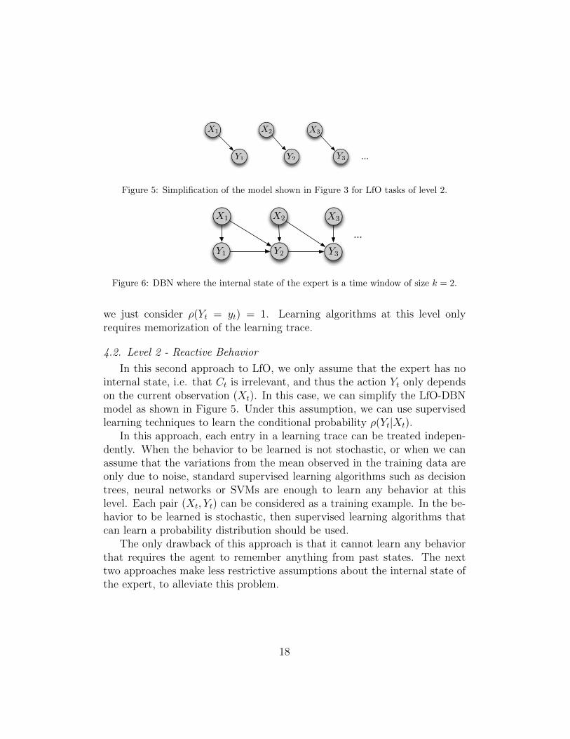
Figure 5: Simplification of the model shown in Figure 3 for LfO tasks of level 2.

X3X1 X2

Y2Y1 Y3

...

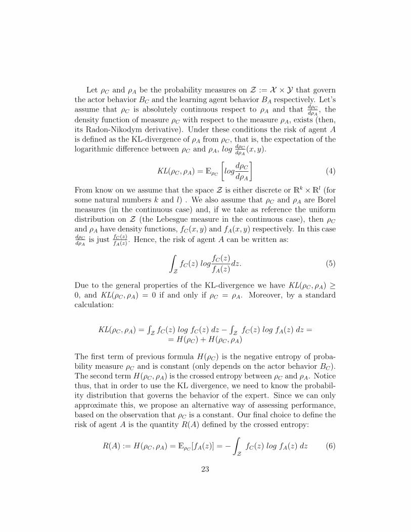
Figure 6: DBN where the internal state of the expert is a time window of size k = 2.

we just consider ρ(Yt = yt) = 1. Learning algorithms at this level onlyrequires memorization of the learning trace.

4.2. Level 2 - Reactive Behavior

In this second approach to LfO, we only assume that the expert has nointernal state, i.e. that Ct is irrelevant, and thus the action Yt only dependson the current observation (Xt). In this case, we can simplify the LfO-DBNmodel as shown in Figure 5. Under this assumption, we can use supervisedlearning techniques to learn the conditional probability ρ(Yt|Xt).

In this approach, each entry in a learning trace can be treated indepen-dently. When the behavior to be learned is not stochastic, or when we canassume that the variations from the mean observed in the training data areonly due to noise, standard supervised learning algorithms such as decisiontrees, neural networks or SVMs are enough to learn any behavior at thislevel. Each pair (Xt, Yt) can be considered as a training example. In the be-havior to be learned is stochastic, then supervised learning algorithms thatcan learn a probability distribution should be used.

The only drawback of this approach is that it cannot learn any behaviorthat requires the agent to remember anything from past states. The nexttwo approaches make less restrictive assumptions about the internal state ofthe expert, to alleviate this problem.

18

x1 y1

x2

x3

x4

x5

y2

y3

y4

y5

Training ExamplesProblem Solution

x1

x2

x3

x4

y1

y2

y3

y4

--

Learning Trace

LT = [ (x1, y1),(x2, y2),(x3, y3),(x4, y4),(x5, y5) ]

Figure 7: Example extraction from a trace. Internal state is a time window with k = 2.

4.3. Restricted Level 3 - Time Window-based Behavior

In this approach, we assume that the expert internal state is a time win-dow memory that stores the last k observations, i.e., the current state Xt,and the last k − 1 observations Ot−1, ..., Ot−(k−1) (which corresponds to thetypical “sliding window” approach [2]). For example, if k = 2, the expertinternal state is Ct = (Xt, Ot−1). Under this assumption we can reformulatethe LfO-DBN model, as shown in Figure 6 for k = 2. Notice that given k, wecan ignore Ct in the DBN model, and thus, we still have no hidden variables.In general, for any given k, the conditional probability that must be learnedis: ρ(Yt|Xt, Ot−1, ..., Ot−(k−1)).

Notice that this is a restricted version of LfO tasks of Level 3. In thisapproach, each subsequence of k entries in a learning trace can be treatedindependently as a training example, and we can still use supervised learningtechniques. Figure 7 shows how training examples for supervised learningcan be extracted from a learning trace under this assumption. The maindrawback of this approach is that, as k increases, the number of features inthe training examples increases, and thus, the learning task becomes morecomplex.

4.4. Level 3 - Memory-based Behavior

In this approach, we only assume that the internal state Ct is discreteand finite. The internal state Ct and the actions Yt at time t depend onthe perceived state of the environment and on the internal state at previousinstants of time. In this situation, the complete LfO-DBN model, as shownin Figure 3 must be considered. The main difference between this approachand the previous two is that now, the supervised learning hypothesis andthe conditional hypothesis p(Ct|xt, ct−1) = p(Ct|xt), might not be true and

19

X3X1 X2

Y2Y1 Y3 ...

X3X1 X2

Y2Y1 Y3

...U1 U2 U3

Hidden Markov ModelInput-Output Hidden Markov Model

Figure 8: A Dynamic Bayesian Network (DBN) representation of Hidden Markov Modelsand Input-Output Hidden Markov Models.

therefore learning traces have to be considered as a whole and cannot bedivided into collections of training examples (Xt, Yt) as before.

A particular case is if we assume that the internal state Ct depends only onprevious internal state Ct−1 and observation Xt. In this case, interestinglyenough, the resulting model shown in Figure 3 corresponds to an Input-Output Hidden Markov Model (IOHMM) [37] (in this case the internal statedepends only on previous inputs, X1, . . . , Xt). IOHMMs are an extensionof Hidden Markov Models (HMM) [38], that can be used to learn how tomap an input sequence to an output sequence (in our case, how to map thesequence of environment observations Xt to actions, Yt). In a standard HMMthere are only two variables: a hidden internal state, typically denoted byx, and an output variable, typically denoted by y. In a IOHMM, there is athird variable u, called input, and both the internal state and the observationvariable depend on u (see Figure 8). In LfO terminology, the internal stateof the IOHMM corresponds to the internal state of the actor, Ct, the outputvariable is the action executed by the expert, Yt, and the input variable (uponwhich the other two depend on) is the observation of the environment stateXt. Learning algorithms for IOHMMs exist for restricted cases. The standardlearning algorithm [37] is derived from the expectation-maximization (EM)algorithm [39] and is applicable as long as the internal state variable Ct isdiscrete (the input (Xt) and action variables (Yt) can be either continuous ordiscrete).

Another particularly interesting case is that in which the input variablesXt are also unobservable, this case is just the well known Hidden MarkovModel (HMM) (as shown in Figure 8).

The main conclusion of this section is that tasks of different levels imposedifferent restrictions from the learning algorithm. Tasks of level 1 require

20

simple memorization, some tasks of level 2 correspond to supervised learning(when behaviors are not stochastic), whereas, in general, tasks of level 3require DBN-style learning algorithms. A specific subclass of behaviors oflevel 3 (those that require only remembering a fixed amount of tie steps) canalso be transformed to level 2 by using a sliding-window approach.

Assuming finite and discrete internal state, we can use EM to learn theparameters of the DBN, but there is no known algorithm to learn the gen-eral class of problems with unrestricted internal state, to the best of ourknowledge. Section 6 presents an empirical evaluation of different algorithmsmaking different assumptions about the internal state. Next section discussesevaluation metrics for LfO algorithms.

5. Evaluation Metrics for LfO

As mentioned before, the evaluation of the performance of LfO algorithmsis still an open problem. In the situation where the task T is known, andthus the learning agent has access to a reward function, evaluation is easier,since we can use the reward function in order to assess the performance ofthe agent, in the same was as in reinforcement learning.

However, when the task T is not specified, the performance of an LfOalgorithm needs to be measured by how much the learned behavior “resem-bles” that of the observed actor. Assessing this “resemblance” is easy or harddepending on the behavior to be learned. In this section, we will present acollection of evaluation metrics that can be used for a range of behaviors.

5.1. Restricted Level 2 - Deterministic Reactive Behavior

When the behavior to be learned is reactive (i. e., it is level 2) and we wantto build a deterministic model for this behavior, we can interpret the behaviorBC of the actor C as a random variable I = (X, Y ) that takes values in X×Y ,where X and Y represent the input and the output variables respectively.In this case, a learning trace LT = [(x1, y1), ..., (xn, yn)] observed by thelearning agent A can be seen as a sample in (X × Y)n, that is, n examplesindependently drawn according to the unknown distribution ρC of variable(X, Y ) that governs the behavior of the actor BC .

A deterministic model for the behavior of agent C is an agent A thatreacts always in the same way if the same input is given. Such a deterministicagent A can be modeled as an input/output map: A : X −→ Y . If we have

21

a loss functions l(y, y′) between actions, then the risk of agent A is definedas the average value of the loss function over the pairs (A(x), y):

R(A) := EρC [l(A(x), y)] =

∫

X×Yl(A(x), y)dρC , (1)

and the goal of learning is to find a model A minimizing the previous riskfunction. As usual, when a trace LTC , generated by the behavior of the actorBC , is given the former theoretical quantity is replaced by the empirical risk

RLTC (A) :=1

n

∑

i=1,...,n

l(A(xi), yi) (2)

If the loss function l : Y × Y −→ R is a 0-1 function, l(y, y′) = I{y}(y′)

(where I{y} is the indicator function), then the (empirical) accuracy of agentA measured using the learning trace LTC is

ACLTC (A) := 1−RLTC (A) = 1− 1

n

∑

i=1,...,n

l(A(xi), yi) (3)

and represents the proportion of actions correctly predicted by agent A. Incase the space of actions Y is discrete we shall use the 0 − 1 loss functionas explained before. If, for instance, actions are represented by real numbers(or vectors of real numbers) the square error loss function could be moreaccurate.

5.2. Level 2 - Stochastic Reactive Behavior

When the behavior to be learned is stochastic, standard empirical risk asdefined in Section 5.1 (or classification accuracy) could not be representativeof the performance of a LfO agent. For example, an agent trying to replicatean actor that executes actions at random would, by definition, have a verylow classification accuracy, even if its behavior is exactly the same as thatof the actor (executing actions at random). For this reason, we need to usean evaluation metric that compares probability distributions over actions,rather than specific actions. Several metrics exist in the literature of Infor-mation Theory. Perhaps the most common strategy for density estimationis based on likelihood principle. Algorithms in this direction try to minimizeKullback-Leibler divergence [40] in the presence of empirical data. For thisreason the metrics that we propose are based on the Kullback-Leibler (KL)divergence.

22

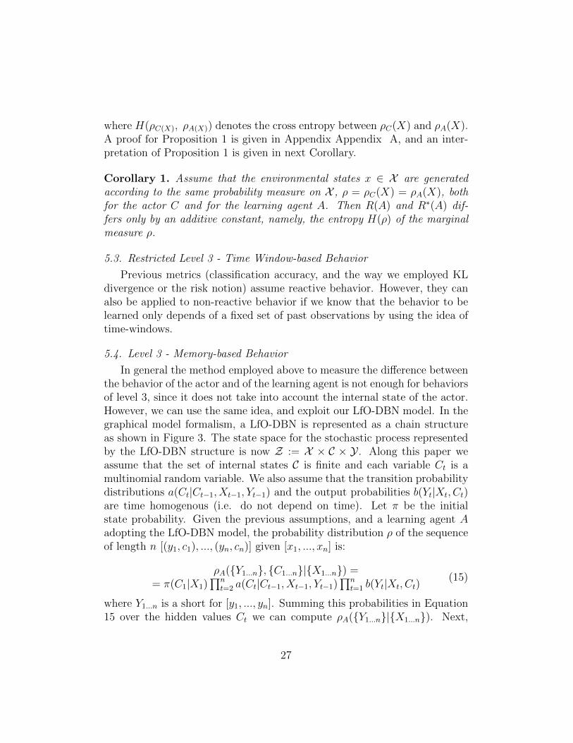
Let ρC and ρA be the probability measures on Z := X × Y that governthe actor behavior BC and the learning agent behavior BA respectively. Let’sassume that ρC is absolutely continuous respect to ρA and that dρC

dρA, the

density function of measure ρC with respect to the measure ρA, exists (then,its Radon-Nikodym derivative). Under these conditions the risk of agent Ais defined as the KL-divergence of ρA from ρC , that is, the expectation of thelogarithmic difference between ρC and ρA, log dρC

dρA(x, y).

KL(ρC , ρA) = EρC

[log

dρCdρA

](4)

From know on we assume that the space Z is either discrete or Rk ×Rl (forsome natural numbers k and l) . We also assume that ρC and ρA are Borelmeasures (in the continuous case) and, if we take as reference the uniformdistribution on Z (the Lebesgue measure in the continuous case), then ρCand ρA have density functions, fC(x, y) and fA(x, y) respectively. In this casedρCdρA

is just fC(z)fA(z)

. Hence, the risk of agent A can be written as:

∫

ZfC(z) log

fC(z)

fA(z)dz. (5)

Due to the general properties of the KL-divergence we have KL(ρC , ρA) ≥0, and KL(ρC , ρA) = 0 if and only if ρC = ρA. Moreover, by a standardcalculation:

KL(ρC , ρA) =∫Z fC(z) log fC(z) dz −

∫Z fC(z) log fA(z) dz =

= H(ρC) +H(ρC , ρA)

The first term of previous formula H(ρC) is the negative entropy of proba-bility measure ρC and is constant (only depends on the actor behavior BC).The second term H(ρC , ρA) is the crossed entropy between ρC and ρA. Noticethus, that in order to use the KL divergence, we need to know the probabil-ity distribution that governs the behavior of the expert. Since we can onlyapproximate this, we propose an alternative way of assessing performance,based on the observation that ρC is a constant. Our final choice to define therisk of agent A is the quantity R(A) defined by the crossed entropy:

R(A) := H(ρC , ρA) = EρC [fA(z)] = −∫

ZfC(z) log fA(z) dz (6)

23

This former definition – sometimes called the Vapnik risk in the related fieldof density estimations [41] – has the advantage that, once we have learnedagent A, the risk of A can be approximated using a Monte Carlo estimationon empirical data, without requiring to know the probability distribution thatgoverns the expert’s behavior. If we have a trace LTC = [z1, . . . , zn] gener-ated according to the actor behavior BC , the Monte Carlo approximation ofEquation 6 is defined as:

RLTC (A) = − 1

n

∑

i=1,...,n

log fA(zi) (7)

Note that, on the other hand, minimizing the previous expression over em-pirical data, corresponds just to the maximum likelihood principle.

It is interesting also to note that sometimes risk estimation can be solvedwithout estimating the densities first (as suggested in Equation 7). For in-stance if the distributions are discrete this intermediate step is unnecessaryand the KL-divergence or the risk can be estimated using directly the empir-ical distributions. To do this it is enough to substitute the distributions ρC(corresponding to the actor behavior) and ρA (corresponding to the learningagent) by their corresponding empirical distributions. Let ρLTC and ρLTA thecorresponding empirical distributions obtained from learning traces LTC andLTA respectively. Recall that if ρ is a discrete probability measure on Z, theempirical probability measure associated to a learning trace LT = [z1, . . . , zn]of size n is defined as:

ρLT (z) :=1

n

n∑

i=1

δzi(z), (8)

where δzi is the Dirach distribution. If f is a real valued function on Z then:

∫

Zf(z)dρLT =

1

n

n∑

i=1

f(zi) (9)

Next, using a trace LTC = [z1, ..., zn] of size n (generated according to theactor behavior) and a trace of size m LTA = [z′1, ..., z

′m] (generated according

to the learning agent behavior), we estimate the risk R(A) defined in Equa-tion 6 by the risk between the empirical distribution of the learning agentρLTA and and the empirical behavior of the actor ρLTA . This leads to thefollowing definition:

24

RLTA,LTC (A) = −∫

Zlog ρLTA(z)dρLTC (10)

If the distributions are discrete, using Equations 8 and 9 we get thefollowing expression:

RLTA,LTC (A) = − 1

n

n∑

i=1

log

[1

m

m∑

j=1

δz′j(zi)

](11)

Strong consistency for the estimator RLTA,LTC (A) is due to the strong law oflarge numbers. Moreover, to improve estimations when the available tracesare too short, or they do not cover the entire Z, we can use Laplace smooth-ing, and modify the equation like this (which is the actual equation we usedin the experiments reported in the next section):

RLTA,LTC (A) = − 1

n

n∑

i=1

log

[1 +

∑mj=1 δz′j(zi)

|Z|+m

](12)

We generalize the previous method to continuous probability measuresas follows. A sample of size n, LTC = [z1, ..., zn], generated according to theactor behavior C, where the zi are vectors of numbers, induces a partitionP of Z in n-dimensional Borel sets by projecting each point zi onto eachcomponent of Z. Next, given a sample of size m generated according to thelearning agent behavior LTA = [z′1, ..., z

′m] we can approximate the empirical

measure ρLTA of each partition element P ∈ P by:

ρLTA(P ) =1

m

m∑

i=1

δz′i(P )

Next, in Equation 11, zi is replaced by P and δz′i(zi) is replaced by δz′i(P )which leads to the following estimator (which could also be adapted to in-corporate Laplace smoothing):

RLTA,LTC (A) = − 1

size(P)

∑

P∈P

log

[1

m

m∑

i=1

δz′i(P )

](13)

25

5.2.1. Estimating Risk from Conditional Distributions

When dealing with reactive behaviors, sometimes it is easier to workwith the conditional probabilities ρC(Y |x) and ρA(Y |x) than with the jointdistribution. In this case, if we have access to a method for generating en-vironmental states (from X ) following a uniform distribution (or any other),then we know the marginal distribution on the the space X , call it ρC(X).The question that naturally arises is which risk function should be used inthis situation. An intuitive answer to this question is to use the expectationof the Kulback-Leibler divergence between the conditional distributions, thatis,

EρC(X)[KL(ρC(Y |x), ρA(Y |x))],

where ρC(Y |x) and ρA(Y |x) are the conditional distributions of actions Ygiven the states X = x of the actor and the learning agent respectively. Theprevious expression can be decomposed into two parts:

−EρC(X)[H(ρC(Y |x))] + EρC(X)[H(ρC(Y |x), ρA(Y |x))].

Due to the previous decomposition, since the first term is constant (i.e. itdoes not depend on the learning agent), our choice for the risk function inthis situation is:

R∗(A) := EρC(X)[H(ρC(Y |x), ρA(Y |x))] == −

∫X fC,X(x)

[∫Y fC,Y |x(y) log fA,Y |x(y) dy

]dx

(14)

where fC,X is the density function of ρC(X) and fC,Y |x is the density functionof ρC(Y |x). We call R∗(A) the conditional distribution risk. We note thisrisk measure with an asterisk, to indicate it is computed from conditionalprobabilities, instead of absolute probabilities, as the risk functions definedbefore. The precise relationship between the quantities R(A) (defined inEquation 6) and R∗(A) (defined in Equation 14) can be established usingBayes and Fubini’s theorems as follows.

Proposition 1. Let BC and BA be the actor an the learning agent behaviorrespectively. Let R(A) and R∗(A) be respectively as before. Then the followingholds:

R(A) = H(ρC(X), ρA(X)) +R∗(A)

26

where H(ρC(X), ρA(X)) denotes the cross entropy between ρC(X) and ρA(X).A proof for Proposition 1 is given in Appendix Appendix A, and an inter-pretation of Proposition 1 is given in next Corollary.

Corollary 1. Assume that the environmental states x ∈ X are generatedaccording to the same probability measure on X , ρ = ρC(X) = ρA(X), bothfor the actor C and for the learning agent A. Then R(A) and R∗(A) dif-fers only by an additive constant, namely, the entropy H(ρ) of the marginalmeasure ρ.

5.3. Restricted Level 3 - Time Window-based Behavior

Previous metrics (classification accuracy, and the way we employed KLdivergence or the risk notion) assume reactive behavior. However, they canalso be applied to non-reactive behavior if we know that the behavior to belearned only depends of a fixed set of past observations by using the idea oftime-windows.

5.4. Level 3 - Memory-based Behavior

In general the method employed above to measure the difference betweenthe behavior of the actor and of the learning agent is not enough for behaviorsof level 3, since it does not take into account the internal state of the actor.However, we can use the same idea, and exploit our LfO-DBN model. In thegraphical model formalism, a LfO-DBN is represented as a chain structureas shown in Figure 3. The state space for the stochastic process representedby the LfO-DBN structure is now Z := X × C × Y . Along this paper weassume that the set of internal states C is finite and each variable Ct is amultinomial random variable. We also assume that the transition probabilitydistributions a(Ct|Ct−1, Xt−1, Yt−1) and the output probabilities b(Yt|Xt, Ct)are time homogenous (i.e. do not depend on time). Let π be the initialstate probability. Given the previous assumptions, and a learning agent Aadopting the LfO-DBN model, the probability distribution ρ of the sequenceof length n [(y1, c1), ..., (yn, cn)] given [x1, ..., xn] is:

ρA({Y1...n}, {C1...n}|{X1...n}) == π(C1|X1)

∏nt=2 a(Ct|Ct−1, Xt−1, Yt−1)

∏nt=1 b(Yt|Xt, Ct)

(15)

where Y1...n is a short for [y1, ..., yn]. Summing this probabilities in Equation15 over the hidden values Ct we can compute ρA({Y1...n}|{X1...n}). Next,

27

we define the n-level conditional distribution risk of agent A (following theLfO-DBN model) with respect to an actor C as:

R∗n(A) = −∫

Xn

[∫

Yn

log ρA({Y1...n}|{X1...n})dρC,T ({Y1...n}|{X1...n})]dρC({X1...n})

(16)

Remark 1. Note that the previous definition is the natural extension of theexpression proposed for R∗(A) for reactive behaviors (Equation 14), but inthis case dealing with the (conditional) distributions over sequences of obser-vations ((X × Y)n), rather than individual observations (Z = X × Y).

Our assumptions about transition and output probabilities, in particularthose assuming the time homogeneous property, implies that the LfO-DBNdefines a stationary process. In this case, the risk rate, defined as:

R∗(A) := limn→∞1

nR∗n(A), (17)

is finite. The risk rate can be used as a (length-independent) risk measure.The LfO-DBN is a 2D-lattice with inhomogeneous field terms (the ob-

served data). It is well known that such kind of structures are intractableusing exact calculations. It is not difficult to write down the EM algorithmgiving the recursions for the calculations of posterior probabilities in the E-step. These calculations are not too time-consuming for practical use (for ntime steps, k values per node the algorithm scales as O(k2n)).

Another important question is how to approximate the risk rate R∗(A)from empirical data. To perform a Monte Carlo approximation of expres-sion 16 we note that a version of Fubini’s theorem states that for any mea-sure ρ on a product space X × Y if we consider the factorization of ρas the marginal measure ρ(X) on X and the conditional measure ρ(Y |x)then for any integrable function φ(x, y) the following holds:

∫φ(x, y) dρ =∫

[∫φ(x, y)dρ(Y |x)]dρ(X). Using Fubini’s theorem in this form, the n-level

risk can be written as:

R∗n(A) = −∫log ρA({Y1...n}|{X1...n})dρ({X1...n}{Y1...n})

28

Level 2:

Classification Accuracy

ACLTC(A) := 1 � 1

n

X

i=1,...,n

l(A(xi), yi)

Monte Carlo approximation of Vapnik's Risk:

Level 3:

Monte Carlo approximation of Vapnik's rate:

Applicable for deterministic reactive behaviors

Applicable for deterministic or stochastic reactive behaviors

Applicable for deterministic or stochastic memory-based

behaviors

RLTA,LTC(A) = � 1

n

nX

i=1

log

24 1

m

mX

j=1

�z0j(zi)

35

R⇤TC

(A) = � 1

|TC |X

T2TC

1

nlog ⇢A({T.Y1...n}|{T.X1...n})

Figure 9: Summary of the different metrics presented in Section 5, where A(xi) representsthe action that the learning agent A would execute when observing xi; δz′

jis Dirac’s

delta function (δz′j(z) = 1 if z = z′j and 0 otherwise); and ρA({T.Y1...n}|{T.X1...n} is

the probability that the learning agent A executed the sequence of actions {T.Y1...n} whenobserving the sequence of observations {T.X1...n} (this probability is estimated by learningan LfO-DBN using traces generated by the learning agent).

Since this last integral is over the joint distribution ρC({X1...n}{Y1...n}), givena set of traces TC of length n generated by the actor C, the Monte Carloapproximation of R∗TC (A) is defined as:

R∗TC (A) = − 1

|TC |∑

T∈TC

1

nlog ρA({T.Y1...n}|{T.X1...n}) (18)

where T.Y1...n represent the sequence of actions the actor executed in traceT , and T.X1...n is the set of observations the actor observed in trace T .

5.5. Summary

Summarizing the definitions and results presented in the previous sub-sections, all the metrics we proposed follow the same general idea: 1) learna probability distribution for the behavior of teach of the agents, 2) use ametric based on the KL-divergence to determine how similar those proba-bility distributions are. The more similar, the better the learning agent has

29

learned. Moreover, instead of using directly the KL-divergence, we use Vap-nik’s risk, which does not require to know the probability distribution thatgoverns the behavior of the expert. For behaviors of level 2, these probabilitydistributions take the form of either absolute distributions of the pair of vari-ables (X, Y ), or conditional probabilities P (Y |X). For behaviors of level 3,these probability distributions take the form of a dynamic Bayesian network,such as the LfO-DBN. Figure 9 presents the list of the evaluation metrics forLfO that we propose, and that will be evaluated in the next section.

6. Experimental Evaluation

This section presents an experimental validation of the theoretical con-cepts put forward in this paper. Specifically we want to evaluate the twomain hypotheses in this paper:

H1: Standard supervised learning metrics for learning algorithm perfor-mance do not correlate well with the performance of LfO algorithms.The proposed metrics put forward in Section 5 better evaluate howclose the behavior of two agents is.

H2: Standard supervised learning algorithms (typically used in many ap-proaches to LfO) can only handle tasks of level 2 that are determinis-tic. For learning stochastic behaviors, or behaviors of level 3, we needa different kind of algorithms.

The following two sections present and discuss a collection of experimentsdesigned to validate these two hypotheses respectively. We used simple do-mains in our evaluation, since those are enough to evaluate whether H1 andH2 hold.

6.1. Performance Evaluation in Learning from Observation

In order to evaluate our proposed metrics, and to show the weaknessesof standard supervised learning metrics (such as classification accuracy) forevaluating how similar is the behavior learned by the learning agent to thatof the actor, we designed the following experiment. We defined a toy domainas follows:

• There are only 3 possible states: X = {x1, x2, x3}.

30

• The agent can only execute 2 actions: Y = {y1, y2}, with deterministiceffect. Action y1 corresponds to moving to the “right” (goes from statex1 to x2, from x2 to x3 and when executed in x3, makes the state goback to x1). Action y2 corresponds to moving to the “left” (from statex1 the action changes the state of x3, from state x2 to x1 and from statex3 to x2).

We defined 8 different agents of several levels with the following behaviors:

SEQ: FixedSequence. (level 1) This agent always repeats the same, fixed,sequence of actions (the sequence is 6 actions long). Once the sequenceis over, it restarts from scratch.

RND: Random. (level 1/2) This agent executes actions at random.

L2DETA: Level 2 Deterministic A. (level 2) This agent produces “right”for states x1 and x2 and “left” otherwise.

L2DETB: Level 2 Deterministic B. (level 2) This agent produces “left”for states x1 and x2 and “right” otherwise.

L2STOA: Level 2 Stochastic A. (level 2) This agent produces, with aprobability 0.75 “right” for states x1 and x2 and “left” for x3. It has aprobability of 0.25 of producing the opposite action.

L2STOB: Level 2 Stochastic B. (level 2) This agent produces, with aprobability 0.75 “left” for states x1 and x2 and “right” for x3. It has aprobability of 0.25 of producing the opposite action.

RNDS: RandomStraight. (level 3) This agent executes one action at ran-dom when in state x1. When in states x2 and x3, it executes the sameaction as in the previous execution cycle with probability 5/6 and theopposite action with probability 1/6.

INT: InternalState. (level 3) This agent has two internal states: i1 andi2 (initially, it starts at i1). When at i1, the agent executes action y1,when at i2, it executes action y2. When the agent observes state x1, itswitches states.

31

Table 2: Comparison of the behavior of different agents using classification accuracy(ACLTC

(A)) (A is the column agent and C is the row agent). The higher, the betterperformance. The highest value in each row is highlighted.

SEQ RND L2DETA L2DETB L2STOA L2STOB RNDS INT

SEQ 1.00 0.52 0.66 0.33 0.59 0.40 0.48 0.50RND 0.53 0.50 0.51 0.49 0.49 0.49 0.51 0.50

L2DETA 0.33 0.53 1.00 0.00 0.74 0.24 0.50 0.50L2DETB 0.33 0.52 0.00 1.00 0.25 0.76 0.50 0.50L2STOA 0.50 0.48 0.75 0.25 0.63 0.39 0.54 0.50L2STOB 0.49 0.50 0.25 0.75 0.38 0.61 0.49 0.48RNDS 0.50 0.51 0.50 0.50 0.48 0.48 0.48 0.49INT 0.33 0.50 0.50 0.50 0.49 0.51 0.47 1.00

We then generated two traces (LT 1A and LT 2

A) of 1000 time steps for eachagent A. We then used performance metrics to determine how well does thebehavior of one agent resemble the behavior of another using these traces.We then compared the behavior of A against C in the following way:

• When using classification accuracy, we take trace LT 2C and feed the

perception state step by step to agent A, asking A to generate thecorresponding action Y . We then use Equation 3 to determine classifi-cation accuracy.

• When using Vapnik’s Risk, we compare traces LT 1A and LT 2

C usingEquation 12.

• When using Vapnik’s rate, we learn an LfO-DBN from trace LT 1A, and

then compute Vapnik’s Risk (Equation 18) with respect to LT 2C .

Ideally, a good performance metric should result in a high score whencomparing an expert with itself, and result in a low score when comparingdifferent experts. Thus, the goal is to validate hypotheses H1 above, and showthat the metrics presented in Section 5 better capture when the behavior oftwo agents is similar than standard supervised learning metrics.

For comparison purposes, we also compared the traces using a standardstatistical test, based on the χ2 distance. The χ2 distance is the underlyingmeasure used in the Pearson statistical hypothesis test. We use it here as ameasure of dissimilarity between probability distributions. For this purpose,we compute the empirical probability distributions ρLTC and ρLTA for Z from

32

Table 3: Comparison of the behavior of different agents using Vapnik’s Risk (RLTA,LTC(A))

(A is the column agent and C is the row agent). The lower, the better performance. Thehighest value in each row is highlighted.

SEQ RND L2DETA L2DETB L2STOA L2STOB RNDS INT

SEQ 1.33 1.81 4.61 6.91 1.75 2.25 1.79 1.79RND 3.23 1.79 4.66 4.89 1.95 1.98 1.79 1.79

L2DETA 1.79 1.85 0.70 6.91 1.24 2.55 1.8 1.79L2DETB 6.91 1.74 6.91 0.70 2.65 1.23 1.79 1.79L2STOA 2.31 1.81 3.15 6.06 1.62 2.28 1.8 1.79L2STOB 4.69 1.77 5.97 3.18 2.31 1.61 1.79 1.79RNDS 3.25 1.79 4.71 4.86 1.97 1.96 1.79 1.79INT 3.27 1.79 4.73 4.84 1.97 1.96 1.79 1.79

Table 4: Comparison of the behavior of different agents using the χ2 distance (A is thecolumn agent and C is the row agent). The lower, the better performance. The highestvalue in each row is highlighted.

SEQ RND L2DETA L2DETB L2STOA L2STOB RNDS INT

SEQ 0.00 61.07 1.98 498.01 11.63 172.48 55.66 55.28RND 0.66 0.00 1.88 2.04 0.28 0.35 0.00 0.00

L2DETA 166.11 102.47 0.00 498.5 36.7 200.46 98.23 96.97L2DETB 277.22 105.56 497.51 0.00 207.98 47.5 110.77 111L2STOA 0.84 0.56 0.7 6.99 0.00 2.26 0.53 0.5L2STOB 1.63 0.45 6.87 0.67 2.17 0.01 0.48 0.51RNDS 0.66 0.01 1.94 2.01 0.31 0.32 0.00 0.00INT 0.66 0.00 1.97 1.98 0.32 0.32 0.00 0.00

traces of both agents, A and C, respectively. Since our experts have discreteaction space Y the χ2 distance is:

χ2(ρLTA , ρLTC ) =∑

y∈Z

(ρLTA(z)− ρLTC (z))2

ρLTC (z)

where quantities ρLTA(z) and ρLTC (z) denote, respectively, the probability ofthe pair observation/action z under measure ρLTA and the probability of zunder measure ρLTC . We use Laplace smoothing to prevent ρLTC (z) beingzero.

Tables 2, 3, 4, and 5 show the results obtained using each of the metricswe used. For each metric, we show a matrix containing one agent per row,and also one agent per column. The number shown in row i and column jrepresents how good agent j approximates the behavior of agent i according

33

Table 5: Comparison of the behavior of different agents using Vapnik’s rate (A is thecolumn agent and C is the row agent). The lower, the better performance. The highestvalue in each row is highlighted.

SEQ RND L2DETA L2DETB L2STOA L2STOB RNDS INT

SEQ 1.33 2.12 36.01 36.04 1.88 2.59 2.01 13.96RND 36.04 1.86 36.04 35.97 2.09 2.24 2.16 29.04

L2DETA 1.81 2.31 0.71 36.04 1.16 3.50 3.72 40.26L2DETB 36.04 1.79 36.04 0.69 2.40 1.08 3.62 22.45L2STOA 36.04 2.05 36.04 36.01 1.65 2.80 2.42 28.55L2STOB 36.04 1.74 36.04 35.87 2.39 1.64 2.56 30.86RNDS 35.83 1.86 36.01 36.04 2.12 2.16 1.66 19.43INT 36.04 1.89 36.04 36.01 2.05 2.14 1.45 1.10

to each metric. Table 2 shows the results computed using standard classi-fication accuracy. For computing classification accuracy, we feed the set ofobservations that row agent observed when generating the test trace to thecolumn agent, recorded the actions the column agent generates and com-pared them against the actions the row agent actually generated. Ideally, wewould like to have numbers close to 1.00 in the diagonal (100% of actionspredicted correctly) and lower anywhere else (since an agent should be ableto properly predict its own actions, but not the actions of other agents).However, we observe that the only elements of the diagonal that are 1.00 arefor agents SEQ, L2DETA, L2DETB, and INT (the agents that are deter-ministic). When agents are not deterministic, classification accuracy is nota good measure of how similar their behaviors are.

Table 3 shows the results using a Monte Carlo approximation of Vapnik’srisk (RLTC ,LTA , shown in Equation 11). Here we expect the values in thediagonal to be lower then all the other values in the same row (notice that wecannot expect zeroes in the diagonal, since the minimum value that Vapnik’srisk can obtain is the entropy of the distribution of the expert H(ρC)). Wecan see that this metric works very well for all the agents of levels 1 and 2.As expected, it is not able to properly distinguish behaviors of level 3 (RNDSand INT). For example, in the rows for the RNDS and INT agents, the valuesobtained by RND, RNDS and INT are almost identical. This metric is thusideal when we know the behaviors of interest are level 2, since it can moreaccurately determine whether an agent’s behavior is similar to another onethan using classification accuracy.

34

-100

-90

-80

-70

-60

-50

-40

-30

-20

-10

0 0

100

200

300

400

500

600

700

800

900

1000

A = SEQ, C = RNDSA = RND, C = RNDS

A = RNDS, C = RNDS

-100

-90

-80

-70

-60

-50

-40

-30

-20

-10

0

0

10

20

30

40

50

60

70

80

90

10

0

A = SEQ, C = RNDSA = RND, C = RNDS

A = RNDS, C = RNDS

Figure 10: An illustration of the convergence of Vapnik’s rate (vertical axis), for differentvalues of n (horizontal axis), computed using Equation 18. Left hand side shows values ofn from 1 to 1000, and the right hand side zooms in to show just the values from 1 to 100.

Table 4 shows the results obtained by using a χ2 test. In this case, wewould like the numbers in the diagonal to be close to 0, and the rest ofnumbers to be high. Notice that indeed the numbers in the diagonal are all0 or very close, but some of the elements outside of the diagonal for the rowsRNDS and INT are also close to 0. Thus, similarly as for Vapnik’s Risk, aχ2 test over the ρLTC and ρLTA distribution can only distinguish the behaviorof agents when they are level 2, but not when they are level 3.

Finally, Table 5 show the results obtained using a Monte Carlo approx-imation to Vapnik’s rate computed using LfO-DBNs. Here we expect thevalues in the diagonal to be lower then all the other values in the same row(again, we cannot expect zeroes in the diagonal, for the same reason as forVapnik’s risk). As we can see, this metric works well for all behaviors, andthe minimum value for each row falls exactly in the diagonal. This meansthat this measure is properly able to determine that the behavior of a givenexpert is most closely predicted by that expert itself.

Finally, Figure 10 illustrates the convergence of the Monte Carlo approxi-mation of Vapnik’s rate used in Table 5 (Equation 18), with increasing valuesof n. Specifically, for n = 1, we consider only the first step of the expert trace,for n = 2 we consider the first two steps, etc. The figure shows the conver-gence of Vapnik’s rate for three specific instances, where the expert was agentRNDS. As we can see, Vapnik’s rte converges to a finite value and, in ourexperiments, it converges to its final value at around n = 200.

The summary is that classification accuracy can only be used to comparebehaviors that are are deterministic, Vapnik’s risk and χ2 over the empiricaldistributions ρLTC and ρLTA over Z can be used for any behavior of Level 2 (or

35

for behaviors that depend only on a fixed set of past states). For behaviorsof level 3, since they require memory, it is not enough with these empiricaldistributions. We need to learn a dynamical model (such as an LfO-DBN)for each agent and then use Vapnik’s rate.

6.2. The Vacuum Cleaner Domain

In order to illustrate the limitations of traditional LfO algorithms, wedesigned a domain that simulates an automatic vacuum cleaner navigating aroom, and removing dirt spots. A scenario is defined as a rectangular grid,where each cell in the grid can be either an empty space, a wall, an obstacle,or dirt. The vacuum cleaner is a 2 by 2 square that navigates the grid lookingfor dirt spots. If the vacuum cleaner enters in contact with a dirt spot, thedirt spot disappears. The goal is to remove all the dirt spots in the map. Forthese experiments, all the obstacles are static, and the only moving object inthe simulation is the vacuum cleaner.

The simulation time is discrete, and at each time step, the vacuum cleanercan take one out of these 5 actions: up, down, left, right and stand still.The effect of the first four actions is to move the vacuum cleaner one cellin each of the four directions, unless there is an obstacle preventing themove (in this case, the vacuum cleaner simple won’t execute the action).Thus, there is a single control variable y, which can take 5 different values:{up,down, left , right , stand}.

The vacuum cleaner perceives the world through 8 different variables,illustrated in Figure 11. Basically, there are 2 variables per direction (up,down, left, right), one of them identifying what can the vacuum cleaner seein each direction (obstacle or dirt), and the other determining whether theobject being seen is close (touching) or far. All the variables are thus binary.The state space of this domain is thus small, but the complexity of it comesfrom the range of behaviors that can be defined, some of which cannot bedescribed as a perception to action mapping.

We hand crafted a collection of 7 different maps, of different sizes, from8x8 to 32x32 and with different configuration of obstacles and dirt. Nextsection presents our experimental results in this domain.

6.3. Comparison of LfO Algorithms

In order to test hypothesis H2, we created eight different agents by hand,that were used as the experts to learn from:

36

x1 = wall (element up)x2 = far (distance)3 di ( l i h )x3 = dirt (element right)x4 = far (distance)x5 = obstacle      (element down)X6 = close (distance)( )x7 = wall  (element left)x8 = close (distance)

Figure 11: The eight variables used as the perception of the environment in our experi-ments.

WF: Wall Follower. (deterministic, level 2) This agent always follows theleft wall. If there is no wall being touched, then it moves right. Theagent is completely deterministic, and has no internal state.

SWF: Smart Wall Follower. (deterministic, level 2) Same as the WF agent,but if it sees dirt in one of the four directions, it will move straight forthe dirt.

RD: Random. (stochastic, level 2) This agent just executes one action atrandom at each cycle.

SRD: Smart Random. (stochastic, level 2) This agent just executes oneaction at random at each cycle, except if it sees dirt in one of the fourdirections, in which case it will move straight for the dirt.

SL: Straight Line. (stochastic, level 3) This agent picks one direction atrandom and moves in a straight line until colliding with an obstacleor a wall. Then it picks a different direction at random, and restartsits behavior. Notice that this behavior has internal state, since thedirection the vacuum cleaner last moved is not included amongst theperception variables X.

SSL: Smart Straight Line. (stochastic, level 3) Like SL, but if it sees dirtin one of the four directions, it will move straight for the dirt. Thisbehavior also has internal state, like SL.

ZZ: Zig-Zag. (deterministic, level 3) This agent moves in zig-zag, it movesall the way to the right, until colliding, then moves down and startsmoving to the left until colliding. When it cannot go down any further,

37

it repeats the behavior, but going up, and so on. In order to properlyperform this behavior, an agent must remember whether it is going leftor right, and also whether it must go down or up after colliding withan object.

SEQ: Fixed Sequence. (deterministic, level 1/3) This agent always loopsover the same, fixed, sequence of actions (15 actions long), indepen-dently of the perception.

We generated a total of 56 learning traces (one per expert per map).We will refer to LTmC to the learning trace generate for agent C in mapm. Therefore, the learning agents have seven learning traces per expert.Each learning trace is 1000 steps long. We compared the performance of thefollowing algorithms:

Supervised Learning Algorithms (level 2): We used NN (Neural Net-works), widely used in the literature of LfO [7, 12], and BN (BayesianNetworks), a direct implementation of the simplified Bayesian Networkshown in Figure 5. Neural Networks in our experiments have one hid-den layer with 10 nodes, and 5 output nodes (one per possible action).

Supervised Learning Algorithms (with time-window-based internalstate, restricted level 3): We also experimented with two algorithmsin this case: NNk2 (Neural Networks) and BNk2 (a direct implementa-tion of the Bayesian Network shown in Figure 6). For both algorithms,we used a time window of size k = 2, i.e. they learn to predict theexpert actions based on the current state of the world, and the stateand action in the previous instant of time.

Dynamic-Bayesian Networks Algorithms (level 3): We experimentedwith using the EM algorithm to learn the parameters of both our pro-posed LfO-DBN model (Figure 3) and a IOHMM. We ran 20 iterationsof the EM algorithm (we used the EM implementation of the BNTsoftware package [42]), and we assumed the internal state of the expertcan take l = 4 different values.

For testing how well a learning method M learns the behavior of an agentC, we used a leave-one-out technique: for each map m, we use method Mto learn behavior from the traces of agent C in all maps except for m. This

38

Table 6: Classification accuracy of different LfO algorithms in predicting the actions ofthe expert. The bottom row shows the average of all the other rows (higher is better; bestperformer per row is highlighted). Right-most column shows the accuracy that the expertitself would achieve in predicting its own actions.

NN NNk2 BN BNk2 LfO-DBN IOHMM Expert

WF 0.99 0.85 0.92 0.86 0.88 0.88 1.00SWF 1.00 0.86 0.94 0.88 0.93 0.93 1.00RD 0.20 0.20 0.21 0.20 0.19 0.19 0.20SRD 0.36 0.34 0.35 0.33 0.36 0.36 0.35SL 0.49 0.93 0.49 0.91 0.79 0.73 0.95SSL 0.49 0.94 0.49 0.92 0.90 0.83 0.94ZZ 0.52 0.96 0.48 0.88 0.83 0.65 1.00SEQ 0.53 0.66 0.40 0.47 0.88 0.65 1.00

Avg. 0.57 0.72 0.54 0.68 0.72 0.65 0.81

results in a learned agent A. We then compared the behavior of A againstC in the following way:

• When using classification accuracy, we take trace LTmC and feed theperception state step by step to agent A, asking A to generate thecorresponding action Y . We then use Equation 3 to determine classifi-cation accuracy.

• When using Vapnik’s Risk, we compare traces LTmA and LTmC usingEquation 12.

• When using Vapnik’s rate, we learn an LfO-DBN from trace LTmA , andthen compute Vapnik’s Risk (Equation 18) with respect to LTmC .

Looking at the classification accuracy results (Table 6), we can see thatNeural Networks (NN), and Bayesian Networks (BN) can predict the be-havior of WF and SWF (which are deterministic and that do not requireinternal memory) very well. Also, we see that when moving to algorithmsbased on time-windows (NNk2, and BNk2), the predictive accuracy improvessignificantly (except for the simple WF and SWF, where NNk2 and BNk2have some overfitting). NNk2 and BNk2 can predict the behavior of the SL,SSL and ZZ experts with very high accuracy. Overall, we see that NNk2,LfO-DBN achieve the highest classification accuracy overall.

Thus, looking at those results, we might believe that NNk2 (neural net-works) performs identically than an LfO-DBN. However, as we showed above,

39

Table 7: Vapnik’s risk between the action distribution predicted by each LfO algorithmand that of the expert, computed based on the current perceptual state xt (lower is better;best performer per row is highlighted). Right-most column shows the Vapnik’s risk withrespect to another set of traces generated by the expert itself.

NN NNk2 BN BNk2 LfO-DBN IOHMM Expert

WF 3.18 4.88 2.93 4.60 2.93 2.94 2.41SWF 2.51 4.95 2.34 4.01 2.15 2.34 2.12RD 8.34 8.56 4.53 6.65 4.55 4.57 4.42SRD 7.37 7.88 3.34 3.93 3.34 3.36 3.31SL 6.35 7.10 3.41 4.65 3.33 3.35 3.29SSL 6.71 7.70 3.07 4.19 3.08 3.11 3.00ZZ 5.65 7.23 3.34 4.25 3.25 3.30 3.16SEQ 7.90 7.93 4.13 5.19 4.13 4.17 3.45

Avg. 6.00 7.03 3.39 4.68 3.34 3.39 3.15

classification accuracy is not representative of how well an LfO agent haslearned a stochastic behavior. Table 7 (showing results using Vapnik’s risk),gives us a better idea of how well the stochastic behaviors (RD, SRD, SL andSSL) where learned. Here we can see that only LfO-DBNs, IOHMMs andBNs learn action distributions that resemble those of the expert.

Table 8 shows a comparison of all the Bayesian models we used in ourexperiments using the Vapnik’s rate (which basically learns an LfO-DBNfrom traces of the learning agent and determines the likelihood of tracesgenerated by the expert according to that LfO-DBN). Vapnik’s rate showsthat there is a significant difference in the performance of BN approaches(BN, BNk2) and DBN ones (LfO-DBN, IOHMM) when learning behaviorsof level 3 (SL, SSL, ZZ). Moreover, LfO-DBNs can learn the behaviors in ourexperiment in a more accurate way than other common DBN models such asIOHMMs. Moreover, we would like to point out that Vapnik’s rate dependon learning an LfO-DBN from traces generated from the learning agent. Thisprocess in itself depends on running the EM algorithm, which might fall intolocal minima. Thus, in order to get a more reliable estimator of Vapnik’srate in practice, it should be computed several times, and keep the minimumvalue obtained. Values in Table 8 represent the minimum obtained aftercomputing Vapnik’s rate twice.

In summary, we can conclude the following: algorithms like Neural Net-works (typically used in the LfO literature) can only learn deterministic be-haviors that do not require memory of past states. Neural Networks can be

40

Table 8: Vapnik’s rate between the action distribution predicted by different LfO algo-rithms and that of the expert, computed based on an LfO-DBN (lower is better). Right-most column shows the Vapnik’s rate with respect to another set of traces generated bythe expert itself.

NN NNk2 BN BNk2 LfO-DBN IOHMM Expert

WF 87.10 184.58 207.02 251.18 85.72 118.63 49.63SWF 148.49 151.48 80.77 228.98 148.13 146.95 43.01RD 252.15 252.22 242.90 252.42 241.50 246.82 220.17SRD 251.54 251.09 235.74 246.48 211.39 243.45 157.17SL 250.45 249.86 240.16 251.38 180.06 181.34 76.46SSL 250.75 249.79 250.83 252.02 184.81 249.69 77.23ZZ 250.83 251.83 247.97 249.73 241.20 215.60 73.97SEQ 252.10 251.85 97.44 221.10 126.07 64.23 24.95

Avg. 217.93 230.34 200.35 244.16 177.36 183.34 90.32

augmented using time windows, which can expand the range of behaviorsthat can be learned, but they are still restricted to deterministic behaviors.Methods like Bayesian Networks can capture stochastic behaviors, but notbehaviors that require memory of past events. Dynamic Bayesian Networkscan learn a wider spectrum of behaviors than other algorithms.

7. Conclusions

Despite the considerable amount of interest and work on learning fromobservation, the field lacks a unified framework for comparing different ap-proaches. The main goal of this paper is to put forward a proposal to fillin that gap, and present a unified framework for learning from observation,consisting of three main components: a) a statistical model which sheds somelight on the formal differences between LfO and other forms of learning, b)a classification of the different levels of difficulty of the tasks attempted byLfO, and c) a collection of evaluation metrics for different LfO tasks. Finally,we have presented an empirical evaluation of our main claims:

1. Supervised learning algorithms are not appropriate for some LfO tasks:our experimental results show that algorithms making different assump-tions can learn different ranges of behaviors, and that supervised learn-ing approaches to LfO are not enough to deal with the general form ofthe LfO problem. Additionally, we compared different approaches to

41

learn from observation: neural networks, bayesian networks and DBNs,and showed their strengths and weaknesses.

2. Our proposed evaluation metrics better reflect the performance of LfOalgorithms than typical metrics used in the literature of LfO: our ex-perimental results show that standard metrics such as classificationaccuracy cannot accurately determine whether two behaviors are sim-ilar or not when these behaviors are stochastic or require memory ofpast states. The alternative metrics proposed in this paper, based Vap-nik’s risk or Vapnik’s rate can better determine behavior similarity inthese situations.

As part of our future work, we want to explore new algorithms to LfOthat can learn the same range of behaviors as our LfO-DBN model, but thatoffer better scalability. Additionally, we would like to continue our study ofperformance metrics for LfO, with the goal of reaching agreement in the LfOcommunity over a set of standard metrics.

Appendix A. Proof of Proposition 1

Proposition 1 in Section 5.2.1 stated that given two agents, BC and BA,then the following holds:

R(A) = H(ρC(X), ρA(X)) +R∗(A)

whereR(A) is the risk measure of the behavior of agentBA with respect to thebehavior of BC when computed from the probability distribution functionsρA and ρC that govern their behaviors, and R∗(A) is the risk when computedfrom the conditional probability distributions. Let us present a proof to suchstatement.

R(A) = −∫

X×YfC(x, y) log(fA(x, y)) dx dy =

= −∫

X×YfC(x, y) log(fA,X(x)fA,Y |x(y)) dx dy =

= −∫

X×YfC(x, y) log(fA,X(x)) dx dy −

∫

X×YfC(x, y) log(fA,Y |x(y)) dx dy

Let’s writeR(A) = R1 +R2,

42

where

R1 = −∫

X×YfC(x, y) log(fA,X(x)) dx dy

and

R2 =

∫

X×YfC(x, y) log(fA,Y |x(y)) dx dy

Let’s analyze each term separately. First,

R1 = −∫

X×YfC(x, y) log(fA,X(x)) dx dy =

= −∫

X

[∫

YfC(x, y) log(fA,X(x) dy

]dx =

= −∫

Xlog fA,X(x)

[∫

YfC(x, y) dy

]dx =

= −∫

XfC,X(x) log fA,X(x) dx = −EρC(X)[fA,X ]

This means that term R1 is the risk of the marginal distribution on com-ponent X, ρA(X) (with respect to the marginal distribution ρC(X) of theactor). The second term R2 can be written as:

R2 = −∫

X×YfC(x, y) log fA,Y |x(y) dx dy =

−∫

X×YfC,X(x) fC,Y |x(y) log fA,Y |x(y) dx dy =

−∫

XfC,X(x)

[∫

YfC,Y |x(y) log fA,Y |x(y) dy

]dx = R∗(A)

�

References

[1] L.-J. Lin, Self-improving reactive agents based on reinforcement learn-ing, planning and teaching, Machine learning 8 (3-4) (1992) 293–321.

[2] T. G. Dietterich, Machine learning for sequential data: A review, in:Proceedings of the Joint IAPR International Workshop on Structural,Syntactic, and Statistical Pattern Recognition, Springer-Verlag, Lon-don, UK, UK, 2002, pp. 15–30.

43

[3] A. V. Nefian, L. Liang, X. Pi, X. Liu, K. P. Murphy, Dynamic bayesiannetworks for audio-visual speech recognition, EURASIP J. Adv. Sig.Proc. 2002 (11) (2002) 1274–1288.

[4] M. A. Bauer, Programming by examples, Artificial Intelligence 12 (1)(1979) 1–21.

[5] T. Lozano-Perez, Robot programming, in: Proceedings of IEEE, Vol. 71,1983, pp. 821–841.

[6] R. S. Michalski, R. E. Stepp, Learning from observation: Conceptualclustering, in: R. S. Michalski, J. G. Carbonell, T. M. Mitchell (Eds.),Machine Learning: An Artificial Intelligence Approach, Tioga, 1983,Ch. 11, pp. 331–364.

[7] D. Pomerleau, Alvinn: An autonomous land vehicle in a neural network,in: D. Touretzky (Ed.), Advances in Neural Information Processing Sys-tems 1, Morgan Kaufmann, 1989.

[8] C. Sammut, S. Hurst, D. Kedzier, D. Michie, Learning to fly, in: ML,1992, pp. 385–393.

[9] T. Sidani, Automated machine learning from observation of simulation,Ph.D. thesis, University of Central Florida (1994).

[10] A. J. Gonzalez, M. Georgiopoulos, R. F. DeMara, A. Henninger, W. Ger-ber, Automating the cgf model development and refinement process byobserving expert behavior in a simulation, in: Proceedings of The 7thConference on Computer Generated Forces and Behavioral Representa-tion, 1998.

[11] H. K. G. Fernlund, A. J. Gonzalez, M. Georgiopoulos, R. F. DeMara,Learning tactical human behavior through observation of human perfor-mance, IEEE Transactions on Systems, Man, and Cybernetics, Part B36 (1) (2006) 128–140.

[12] C. L. Moriarty, A. J. Gonzalez, Learning human behavior from obser-vation for gaming applications, in: FLAIRS Conference, 2009.

[13] D. C. Bentivegna, C. G. Atkeson, Learning from observation using prim-itives, in: In IEEE International Conference on Robotics and Automa-tion, 2001, pp. 1988–1993.

44

[14] S. Chernova, M. M. Veloso, Confidence-based policy learning fromdemonstration using gaussian mixture models, in: AAMAS, 2007, p.233.

[15] S. Chernova, M. M. Veloso, Teaching multi-robot coordination usingdemonstration of communication and state sharing, in: AAMAS, 2008,pp. 1183–1186.

[16] S. Schaal, Learning from demonstration, in: NIPS, 1996, pp. 1040–1046.

[17] C. G. Atkeson, J. G. Hale, F. E. Pollick, M. Riley, S. Kotosaka, S. Schaal,T. Shibata, G. Tevatia, A. Ude, S. Vijayakumar, M. Kawato, Usinghumanoid robots to study human behavior, IEEE Intelligent Systems15 (4) (2000) 46–56.

[18] B. D. Argall, S. Chernova, M. Veloso, B. Browning, A survey of robotlearning from demonstration, Robot. Auton. Syst. 57 (2009) 469–483.doi:10.1016/j.robot.2008.10.024.

[19] T. Konik, J. E. Laird, Learning goal hierarchies from structured obser-vations and expert annotations, Mach. Learn. 64 (1-3) (2006) 263–287.doi:http://dx.doi.org/10.1007/s10994-006-7734-8.

[20] R. Khardon, Learning to take actions, Mach. Learn. 35 (1) (1999) 57–90.doi:10.1023/A:1007571119753.

[21] M. W. Floyd, B. Esfandiari, K. Lam, A case-based reasoning approachto imitating robocup players, in: Proceedings of the Twenty-First In-ternational Florida Artificial Intelligence Research Society (FLAIRS),2008, pp. 251–256.

[22] S. Ontanon, K. Mishra, N. Sugandh, A. Ram, Case-based planning andexecution for real-time strategy games, in: ICCBR, 2007, pp. 164–178.

[23] S. Ontanon, K. Mishra, N. Sugandh, A. Ram, On-line case-based plan-ning, Computational Intelligence Journal 26 (1) (2010) 84–119.

[24] S. Ontanon, Case acquisition strategies for case-based reasoning in real-time strategy games, in: FLAIRS Conference, 2012.

[25] J. Rubin, I. Watson, On combining decisions from multiple expert imi-tators for performance, in: IJCAI, 2011, pp. 344–349.

45

[26] L. Lamontagne, F. Rugamba, G. Mineau, Acquisition of cases in se-quential games using conditional entropy, in: ICCBR 2012 Workshopon TRUE: Traces for Reusing Users’ Experience, 2012.

[27] A. Y. Ng, S. Russell, Algorithms for Inverse Reinforcement Learning,in: in Proc. 17th International Conf. on Machine Learning, 2000, pp.663–670.

[28] E. Klein, M. Geist, O. Pietquin, Batch, off-policy and model-free appren-ticeship learning, in: IJCAI Workshop on Agents Learning Interactivelyfrom Human Teachers (ALIHT 2011), Barcelona (Spain), 2011.

[29] M. Lopes, T. Cederbourg, P.-Y. Oudeyer, Simultaneous acquisition oftask and feedback models, in: IJCAI Workshop on Agents LearningInteractively from Human Teachers (ALIHT 2011), Barcelona (Spain),2011.

[30] B. Tastan, G. R. Sukthankar, Learning policies for first person shootergames using inverse reinforcement learning, in: AIIDE, 2011.

[31] E. W. Dereszynski, J. Hostetler, A. Fern, T. G. Dietterich, T.-T. Hoang,M. Udarbe, Learning probabilistic behavior models in real-time strategygames, in: AIIDE, 2011.

[32] A. Pentland, A. Liu, Toward augmented control systems, in: Proceed-ings of the Intelligent Vehicles ’95 Symposium, 1995, pp. 350–355.

[33] E. Billing, T. Hellstrom, A formalism for learning from demonstration,Paladyn Journal of Behavioral Robotics 1:1, s. 1-13.

[34] C. L. Johnson, A contextual approach to learning collaborative behaviorvia observation, Ph.D. thesis, University of Central Florida Orlando,Florida (2011).

[35] A. Papoulis, S. U. Pillai, Probability, Random Variables, and StochasticProcesses, McGraw-Hill Series in Electrical and Computer Engineering,McGraw-Hill, 2002.

[36] Z. Ghahramani, Learning dynamic bayesian networks, in: Adaptive Pro-cessing of Sequences and Data Structures, International Summer Schoolon Neural Networks, ”E.R. Caianiello”-Tutorial Lectures, Springer-Verlag, London, UK, 1998, pp. 168–197.

46

[37] Y. Bengio, P. Frasconi, Input/output hmms for sequence processing,IEEE Transactions on Neural Networks 7 (1996) 1231–1249.

[38] L. R. Rabiner, A tutorial on hidden markov models and selected appli-cations in speech recognition, in: Proceedings of the IEEE, 1989, pp.257–286.

[39] A. P. Dempster, N. M. Laird, D. B. Rubin, Maximum likelihood fromincomplete data via the em algorithm, Journal of the Royal StatisticalSociety, Series B 39 (1) (1977) 1–38.

[40] S. Kullback, R. A. Leibler, On information and sufficiency, Ann. Math.Statist. 22 (1) (1951) 79–86.

[41] V. Vapnik, The nature of Statistical Learning Theory, Springer Verlag,1995.

[42] K. Murphy, The bayes net toolbox for matlab, Computing science andstatistics 33 (2) (2001) 1024–1034.

47