University of WollongongResearch Online

Faculty of Commerce - Papers Faculty of Commerce

2007

Dynamic linkages between Thai and internationalstock marketsAbbas ValadkhaniUniversity of Wollongong, abbas@uow.edu.au

S. ChancharatUniversity of Wollongong, sc983@uow.edu.au

Research Online is the open access institutional repository for theUniversity of Wollongong. For further information contact ManagerRepository Services: morgan@uow.edu.au.

Recommended CitationValadkhani, Abbas and Chancharat, S.: Dynamic linkages between Thai and international stock markets 2007.http://ro.uow.edu.au/commpapers/354

Dynamic linkages between Thai and international stock markets

AbstractThis paper investigates the existence of cointegration and causality between the stock market price indices ofThailand and its major trading partners (Australia, Hong Kong, Indonesia, Japan, Korea, Malaysia, thePhilippines, Singapore, Taiwan, the UK and the US), using monthly data spanning December 1987 toDecember 2005. Both the Engle-Granger two-step procedure (assuming no structural breaks) and theGregory and Hansen (1996) test (allowing for one structural break) provide no evidence of a long-runrelationship between the stock prices of Thailand and these countries. Based on the empirical results obtainedfrom these two residual-based cointegration tests, potential long-run benefits exist from diversifying theinvestment portfolios internationally to reduce the associated systematic risks across countries. However, inthe short run, three unidirectional Granger causalities run from the stock returns of Hong Kong, thePhilippines and the UK to those of Thailand, pair-wise. Furthermore, there are two unidirectional causalitiesrunning from the stock returns of Thailand to those of Indonesia and the US. We also found empiricalevidence of bidirectional Granger causality, suggesting that the stock returns of Thailand and three of itsneighbouring countries (Malaysia, Singapore and Taiwan) are interrelated. No previous study examines thepossibility that the pair-wise long-run relationship between the stock prices of Thailand and those of bothemerging and developed markets may have been subject to a structural break.

Keywordsthailand, stock markets, cointegration, structural breaks

Publication DetailsThis article originally published as: Valadkhani, A, and Chancharat, S, Dynamic Linkages between Thai andInternational Stock Markets, Journal of Economic Studies, 2008, in press (accepted 17 August 2007).Copyright Emerald 2008. Original journal information available here.

This journal article is available at Research Online: http://ro.uow.edu.au/commpapers/354

1

Dynamic linkages between Thai and international

stock markets

Abbas Valadkhani and Surachai Chancharat School of Economics, University of Wollongong, NSW 2522 Australia

This paper investigates the existence of cointegration and causality between the stock market price indices of Thailand and its major trading partners (Australia, Hong Kong, Indonesia, Japan, Korea, Malaysia, the Philippines, Singapore, Taiwan, the UK and the US), using monthly data spanning December 1987 to December 2005. Both the Engle-Granger two-step procedure (assuming no structural breaks) and the Gregory and Hansen (1996) test (allowing for one structural break) provide no evidence of a long-run relationship between the stock prices of Thailand and these countries. Based on the empirical results obtained from these two residual-based cointegration tests, potential long-run benefits exist from diversifying the investment portfolios internationally to reduce the associated systematic risks across countries. However, in the short run, three unidirectional Granger causalities run from the stock returns of Hong Kong, the Philippines and the UK to those of Thailand, pair-wise. Furthermore, there are two unidirectional causalities running from the stock returns of Thailand to those of Indonesia and the US. We also found empirical evidence of bidirectional Granger causality, suggesting that the stock returns of Thailand and three of its neighbouring countries (Malaysia, Singapore and Taiwan) are interrelated. No previous study examines the possibility that the pair-wise long-run relationship between the stock prices of Thailand and those of both emerging and developed markets may have been subject to a structural break. Keywords Stock markets, Cointegration, Structural breaks, Thailand Paper type Research paper

1. Introduction

There are many reasons why stock markets of different countries may have significant co-movements. For example global capital movements and the presence of economic ties and regional policy coordination among countries can directly or indirectly interconnect their stock prices through time. According to Phylaktis and Ravazzolo (2005), unlike other crises, the Asian crisis engulfed a group of countries that were both financially and economically integrated prior to the crisis. However, Chan et al. (1997) argue that although common economic and geographic factors were considered as crucial factors, they were not necessarily major causes of national stock markets to follow the same stochastic trend. It is also argued that there is less evidence of stock market integration after major stock market crises and hence international diversification among stock markets can be undertaken more effectively due to the lack of long-run co-movements of international stock prices (Patev et al., 2006). In the context of the Malaysian stock market, for example, Ibrahim and Aziz (2003) provide

2

some evidence that the Asian crisis appears to give rise to irregularity in the interactions between stock prices and macroeconomic variables.

A growing interest in the integration of international stock markets is evident in the number of empirical studies that examine the various aspects of stock market linkages. These studies were mainly motivated by the stock market crash in October 1987 and subsequent Asian financial crisis in 1997. For instance, Susmel and Engle (1994), Fraser and Power (1997), Kanas (1998b) and Fratzscher (2002) examine volatility spillovers across stock markets; while Phylaktis and Ravazzolo (2002) report their test results using international capital asset pricing models.

In addition to these studies, cointegration techniques in the literature are widely used to investigate the long-run relationships between stock markets. These studies can be classified into three groups. First, some focus mainly on developed markets in the US, Canada, Europe and Japan (for example, Kasa, 1992; Richards, 1995; Choudhry, 1996; Kanas, 1998a; Hamori and Imamura, 2000; Ahlgren and Antell, 2002) and find some evidence that there are interdependent linkages among the stock markets of developed countries. Second, other studies in the literature examine the stock price linkages among only emerging stock markets, without capturing the important influence of stock markets in developed countries. They find only weak evidence of a relationship among the Asian stock markets (for more details see Chaudhuri, 1997; Sharma and Wongbangpo, 2002; Worthington et al., 2003; Yang et al., 2003).

The last group of studies examines the interdependencies between developed and emerging markets but they do not incorporate the effect of possible structural changes in the long-run relationships, such as the 1987 great crash and the Asian financial crisis in 1997. Due to earlier inconclusive results, there is no consensus among previous studies as to whether international stock markets are interdependent. For instance, while Masih and Masih (1999) and Syriopoulos (2004) found some pair-wise long-run relationships between stock markets in developed countries and the stock markets of emerging countries, other studies (such as Chang, 2001; Ng, 2002; Climent and Meneu, 2003) do not find any empirical evidence suggesting that stock market dependence exists among such countries. These studies have deepened our understanding of the interplay among international stock market linkages; however, allowing for a possible break in cointegration vectors, this paper specifically examines the interplay between the stock markets in Thailand and 11 other countries, including both developed and emerging markets.

Compared to previous studies, this paper differs in two aspects. First, no previous study examines the possibility that the pair-wise long-run relationship between the stock prices of two countries may have been subject to a structural break. In addition to the Engle–Granger two-step procedure, this paper employs the Gregory and Hansen (GH, 1996) cointegration test, which allows for a structural break in the cointegrating vector. Gregory and Hansen argue that structural breaks have important implications for cointegration analysis because these breaks can decrease the power of cointegration tests and lead to the under-rejection of the null hypothesis of no cointegration.

Second, as discussed earlier, most previous studies focus on developed markets, and few examine both emerging and developed markets. In contrast, this study examines whether the Thai stock market is linked with the stock markets of its major trading partners. No existing study focuses specifically on the Thai stock market, although some include Thailand in their sample countries (for example, Masih and

3

Masih, 1999; Chang, 2001; Ng, 2002; Sharma and Wongbangpo, 2002; Climent and Meneu, 2003; Worthington et al., 2003; Phylaktis and Ravazzolo, 2005).

The 1997 Asian financial crisis first began with the floating of the Thai baht in July 1997, and soon after, the crisis spread rapidly to the Philippines, Malaysia, Indonesia and Korea. Following this crisis, relatively small depreciations also engulfed Singapore and Japan (Barro, 2001). Therefore, Thailand can be considered as an important case among other emerging markets. In 2004, on the Stock Exchange of Thailand (SET), market turnover was 93.8 per cent, there were 465 listed domestic companies, and the value traded was $US109,949 million. The SET was classified as the ninth highest among emerging markets in terms of these three measures, and the nineteenth, twentieth and twenty-fourth on a global scale. In terms of market capitalisation, the SET reached a record high $US115,400 million, which ranked twelfth-highest among all emerging markets and thirty-first in the world (Standard and Poor’s, 2005).

This paper investigates the long-run and short-run relationships between the Thai stock market and those of its major trading partners: Australia, Hong Kong, Indonesia, Japan, Korea, Malaysia, the Philippines, Singapore, Taiwan, the UK and the US. We chose these eleven countries because of their relatively high share of Thai exports and imports. It should be noted that Japan and the US are Thailand’s two biggest trading partners. Malaysia, Singapore, Indonesia and the Philippines are all members of the Association of Southeast Asian Nations (ASEAN), which aims to remove trade barriers among its member countries. Hong Kong, Taiwan and Australia are also among Thailand’s top-ten trading partners, followed by Korea and the UK, which are just outside the top ten.

The remainder of the paper is structured as follows. Section 1 discusses briefly the empirical methodology adopted in the paper. Section 2 describes the summary statistics of the data. Section 3 presents the empirical results of cointegration and causality tests. Finally, Section 4 provides some concluding remarks.

2. Empirical methodology

We initially performed the augmented Dickey-Fuller (ADF) unit root test to examine the time series properties of the data without allowing for any structural breaks. The ADF test is conducted using this equation:

t

k

i

ititt ycyty εαβµ +∆+++=∆ ∑=

−−

1

1 (1)

Where yt denotes the time series being tested; ln( )i

t ty P= , ln( )i

tP is the natural

logarithm of the stock market price index in country i; ∆ is the first different operator; t

is a time trend term; k denotes the optimal lag length; and ε t is a white noise disturbance term.

In this paper, the lowest value of the Akaike information criterion (AIC) was used as a guide to determine the optimal lag length in the ADF regression. These lags augment the ADF regression to ensure that the error term is white noise and free of serial correlation. In addition, the Phillips-Perron (PP) test was used as an alternative nonparametric model to control for serial correlation. Using the PP test ensures that the higher-order serial correlations in the ADF equation were handled properly. That is, the ADF test corrects for higher-order autocorrelation by including lagged differenced terms on the right-hand side of the ADF equation; whereas the PP test corrects the ADF t-statistic by removing the serial correlation in it. This nonparametric t-test uses the

4

Newey-West heteroscedasticity autocorrelation consistent estimate, and is robust to heteroscedasticity and autocorrelation of unknown form.

An important shortcoming associated with the ADF and PP tests is that they do not allow for the effect of structural breaks. Perron (1989) argues that if a structural break in a series is ignored, unit root tests can be erroneous in rejecting null hypothesis. Zivot and Andrews (ZA, 1992) developed methods to search endogenously for a structural break in the data. We employ their ‘model C’, which allows for one structural break in both the intercept and slope coefficients in the following equation:

t

k

i

ititttt ycyDTDUty εαγθβµ +∆+++++=∆ ∑=

−−

1

1 (2)

Where 1=tDU if TBt > , otherwise zero; TB denotes the time of break; and

TBtDTt −= if TBt > , otherwise zero.

The ‘trimming region’, in which we searched for TB covers the 0.15T-0.85T period, where T is the sample size. Following Chaudhuri and Wu (2003) and Narayan and Smyth (2005), we selected the break point (TB) based on the minimum value of the t

statistic for α. In this study, kmax is set equal to 12. After determining the order of integration of each variable, we needed to test for the

existence of any long-run relationship between the stock prices of Thailand and its major trading partners. We employed the Engle-Granger two-step procedure first by obtaining the resulting residuals of the following equation, and then conducting a unit root test on them:

0t t ty t xµ β ϕ ε= + + + (3)

Where yt and xt are the natural log of the stock price indices of Thailand and one of its major trading partners, respectively.

According to Engle and Granger (1987), if both yt and xt are I(1), and t̂ε is I(0),

then a long-run relationship between these two variables exists. The resulting error-correction model (ECM) from such a model can then be written as:

1 2

1

0 1

k k

t i t i i t i t t

i i

y x y ECM vφ λ δ η− − −

= =

∆ = + ∆ + ∆ + +∑ ∑ (4)

Whereisλ

are the estimated short-term coefficients;

isδ denotes the estimated

coefficients of the lagged dependent variables added to ensure vt or the disturbance term is white noise; η is the feedback effect capturing the speed of adjustment, whereby

short-term dynamics converge to the long-term equilibrium path indicated in equation

(3); and ECMt or t̂ε is obtained from equation (3) by the OLS method.

The general-to-specific methodology can then be used to omit insignificant variables in equation (4) based on a battery of maximum likelihood tests. In this method joint zero restrictions are imposed on explanatory variables in the unrestricted (general) model to obtain a parsimonious model. The null hypothesis of no cointegration is rejected if 0η < and is statistically significant.

The lack of evidence of cointegration in previous studies in the literature could be attributed to the ignorance of the structural break in cointegrating vector. To address this issue, we also used the GH (1996) test. GH (1996) postulate three alternative models similar to those proposed by ZA (1992) to capture the changes in parameters of the cointegrating vector. First, the level shift model (C), which assumes a change only in the intercept, as shown below:

5

0 1t t t ty DU xµ θ µ ε= + + + (5)

The second model, a level shift and change in trend (C/T), takes this form:

0 1t t t ty DU t xµ θ β µ ε= + + + + (6)

The third model, which allows for changes in both the intercept and slope of the cointegration vector (C/S), is presented as:

0 1 2t t t t t ty DU t x x DUµ θ β µ µ ε= + + + + + (7)

Where t

DU is defined as previously in equation (2).

Intuitively, within the range of 0.15T-0.85T, this technique searches for a particular

TB, which minimises the value of the ADF* statistic for t̂ε . The GH (1996) method tests

the null hypothesis of no cointegration against the alternative hypothesis of cointegration with a single structural break at time TB, which is determined endogenously.

Finally, we conducted the Granger causality test based on the error correction

model specified in equation (4). A variable such as t

x∆ (the stock returns) Granger

causes t

y∆ if its past values can explain

ty∆ , but past values of

ty∆

do not explain

tx∆

(Granger, 1969). If the two variables are not cointegrated, and η in equation (4) is not

negative and significant, the following bivariate VAR equations will then be used for the causality test:

1 2

0

1 1

k k

t t i t i i t i t

i i

y x x y vφ λ λ δ− −

= =

∆ = + ∆ + ∆ + ∆ +∑ ∑ (8)

1 2

0

1 1

k k

t t i t i i t i t

i i

x y y x vφ λ λ δ′ ′

− −

= =

′ ′ ′ ′ ′∆ = + ∆ + ∆ + ∆ +∑ ∑ (9)

On the other hand, if yt and xt are cointegrated, these error correction models are adopted:

1 2

0 1

1 1

k k

t t i t i i t i t t

i i

y x x y ECM vφ λ λ δ η− − −

= =

∆ = + ∆ + ∆ + ∆ + +∑ ∑ (10)

1 2

0 1

1 1

k k

t t i t i i t i t t

i i

x y y x ECM vφ λ λ δ η′ ′

− − −

= =

′ ′ ′ ′ ′ ′∆ = + ∆ + ∆ + ∆ + +∑ ∑ (11)

The Granger causality test can be conducted under two assumptions. First, if yt and xt are not cointegrated, then we can use equations (8) and (9) to test the following two null

hypotheses: If in equation (8) 1 2 1: ... 0o k

H λ λ λ= = = =

is rejected, then

1ln lnj j

t t tx P P−∆ = − , or the stock price return in country j, Granger causes

1ln lni i

t t ty P P−∆ = − or the stock price return in country i. This can be written as

t tx y∆ → ∆ . Similarly, if, in equation (9), 1 2 1: ... 0

o kH λ λ λ′ ′ ′ ′= = = = is rejected, then we

can conclude that t

y∆ causes t

x∆ or t t

y x∆ → ∆ . If both null hypotheses are rejected

simultaneously, there would be a bidirectional causality between the two variables, that

is, t t

y x∆ ↔ ∆ . Second, if yt and xt are in fact cointegrated, then we need to use

equations (10) and (11) to test the same two hypotheses. The inclusion of ECM in these two equations ensures that the long-term run properties of the data are not lost when

dealing with the first difference form. If in equation (10), 1 2 1: ... 0o k

H λ λ λ= = = = is

rejected, then t t

x y∆ → ∆ (

tx∆

Granger causes

ty∆ ), or

t tx y∆ → ∆ . In the same way, if

6

in equation (11), 1 2 1: ... 0o k

H λ λ λ′ ′ ′ ′= = = = is rejected, then one can conclude that

t ty x∆ → ∆ . If both

oH and

oH ′ are rejected, the causality between the two variables is

bidirectional, or t t

y x∆ ↔ ∆ .

3. Data and summary statistics

The data included in this paper include the stock prices of these 12 countries: Thailand (TH), Australia (AU), Hong Kong (HK), Indonesia (IN), Japan (JA), Korea (KO), Malaysia (MA), the Philippines (PH), Singapore (SG), Taiwan (TA), the UK and the US. Monthly data span December 1987 to December 2005, with a base value of 100 in December 1987. All stock price indices were obtained from Morgan Stanley Capital International (MSCI) which is one of the widely used sources of financial data in the literature (Hamori and Imamura, 2000; Ahlgren and Antell, 2002; Ng, 2002; Climent and Meneu, 2003; Worthington et al., 2003) in terms of the degree of comparability and avoidance of dual listings. Since this paper is concerned with the comparative performance of the international stock markets, all price indices (P) are denominated in US dollars. The MSCI indices for different markets are computed using the same consistent formula which is value weighted. The rate of returns ln(Pt/Pt-1) calculated from the MSCI price indices which consists of both capital gain and income gain .

[Table I about here]

Table I presents the descriptive statistics of the data, including sample means, medians, maximums, minimums, standard deviations, skewness, kurtosis as well as the Jarque-Bera statistics and p-values. The highest mean return is 0.008 per cent in Hong Kong and the US while the lowest is 0.000 per cent in Japan. The standard deviations range from 0.041 per cent in the US (the least volatile) to 0.145 per cent in are Indonesia (the most volatile). The standard deviations of stock returns are lowest in developed economies (that is, the US, the UK, Australia and Japan), and the most volatile in Indonesia, Thailand, Taiwan and Korea. All monthly stock returns,

1ln( / )t t

P P− , have excess kurtosis, which means that they have a thicker tail and a higher

peak than a normal distribution. The calculated Jarque-Bera statistics and corresponding p-values are used to test for the normality assumption. Based on the Jarque-Bera statistics and p-values, this assumption is rejected at any conventional level of significance for all stock returns, with the only three exceptions being the monthly stock returns in Australia, Japan and the UK.

4. Empirical results

As mentioned earlier, we first used the ADF and PP tests to determine the order of integration of the 12 stock prices studied. The lowest value of the AIC was used to determine the optimal lag length in the estimation procedure. Based on the results of the unit root tests presented in Table II, the ADF and PP tests reject the random walk hypothesis for only the stock price index in Taiwan at the five and one per cent significance levels, respectively. However, for all other countries, both unit root tests cannot reject the random walk hypothesis. We thus conclude that the stock price indices in 11 out of the 12 countries are I(1).

[Table II about here]

In the second stage, we subjected each variable to one structural break. For each series, we then carried out the ZA test (model C) and report the results in Table III, below. As mentioned earlier, the ADF and PP test results reveal that most stock prices

7

examined in this paper followed a random walk; whereas the results of the ZA test show that stock prices for three countries (that is, Indonesia, Korea and Malaysia) are now stationary. Despite allowing for one endogenous structural break in the data, the data in

the remaining nine countries still contain a unit root. The estimated coefficients µ and θ

are statistically significant for all variables, except for θ in the case of the Philippines stock prices. There was at least one structural break in the intercept during the sample

period for all stock prices. The estimated coefficients for β and γ are also statistically significant in eight and nine out of 12 countries, respectively, implying the stock price series exhibits an upward or downward trend and at least one structural break in trend in these countries exists.

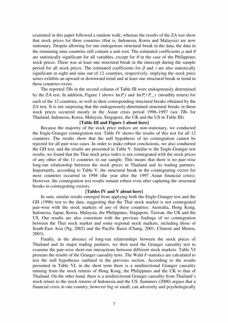
The reported TBs in the second column of Table III were endogenously determined

by the ZA test. In addition, Figure 1 shows ln( )t

P and 1ln( / )t t

P P− (monthly return) for

each of the 12 countries, as well as their corresponding structural breaks obtained by the ZA test. It is not surprising that the endogenously-determined structural breaks in these stock prices occurred mostly in the Asian crisis period 1996–1997 (see TBs for Thailand, Indonesia, Korea, Malaysia, Singapore, the UK and the US in Table III).

[Table III and Figure 1 about here]

Because the majority of the stock price indices are non-stationary, we conducted the Engle-Granger cointegration test. Table IV shows the results of this test for all 12 countries. The results show that the null hypothesis of no cointegration cannot be rejected for all pair-wise cases. In order to make robust conclusions, we also conducted the GH test, and the results are presented in Table V. Similar to the Engle-Granger test results, we found that the Thai stock price index is not cointegrated with the stock prices of any other of the 11 countries in our sample. This means that there is no pair-wise long-run relationship between the stock prices in Thailand and its trading partners. Importantly, according to Table V, the structural break in the cointegrating vector for most countries occurred in 1998 (the year after the 1997 Asian financial crisis). However, the cointegration test results remain robust even after capturing the structural breaks in cointegrating vectors.

[Tables IV and V about here]

In sum, similar results emerged from applying both the Engle-Granger test and the GH (1996) test to the data, suggesting that the Thai stock market is not cointegrated pair-wise with the stock markets of any of these countries: Australia, Hong Kong, Indonesia, Japan, Korea, Malaysia, the Philippines, Singapore, Taiwan, the UK and the US. Our results are also consistent with the previous findings of no cointegration between the Thai stock market and some regional stock markets, including those of South-East Asia (Ng, 2002) and the Pacific Basin (Chang, 2001; Climent and Meneu, 2003).

Finally, in the absence of long-run relationships between the stock prices of Thailand and its major trading partners, we then used the Granger causality test to examine the pair-wise short-run interactions between different stock markets. Table VI presents the results of the Granger causality tests. The Wald F-statistics are calculated to test the null hypotheses outlined in the previous section. According to the results presented in Table VI, in the short term there is a unidirectional Granger causality running from the stock returns of Hong Kong, the Philippines and the UK to that of Thailand. On the other hand, there is a unidirectional Granger causality from Thailand’s stock return to the stock returns of Indonesia and the US. Summers (2000) argues that a financial crisis in one country, however big or small, can adversely and psychologically

8

affect investors’ perceptions and expectations in other countries. Investors’ reactions to acute market shocks when coincided with unwise government policy responses can influence the other markets. For example the Asian crisis influenced the other stock markets in the world (including the US market) as investors started panicking that the financial downturn could also engulf their market due to knock-on effects across international markets. This could partially explain why the stock market return in such a small country such as Thailand Granger causes the return in the US market.

We also found a bidirectional Granger causality between the market stock returns in Thailand and its three neighbouring countries (that is, Malaysia, Singapore and Taiwan). Therefore, the short-run movements of stock returns in these three countries can influence the performance of Thailand’s stock market. It can also be concluded that any short-run variation of the stock returns in Thailand can affect the market returns of its three neighboring countries, and vice versa. Hence, in order to avoid financial contagion and future crises similar to the one which occurred in 1997, central bankers and individual investors must keep abreast of new developments in international stock markets — particularly those for which we found the evidence of bidirectional and unidirectional causality.

[Table VI about here]

5. Conclusions

This study examines the long-run and short-run relationships between the stock prices of Thailand and its major trading partners (Australia, Hong Kong, Indonesia, Japan, Korea, Malaysia, the Philippines, Singapore, Taiwan, the UK and the US), using monthly data for the period December 1987 to December 2005. In addition to the Engle-Granger two-step procedure, we used the Gregory and Hansen (1996) test, which allows for a structural break in the cointegration vector.

Based on the cointegration results, we found no evidence of long-run relationships between the stock price indices of Thailand and its major trading partners. The policy implication of this finding for international investors is quite straightforward: in the long run, there are potential gains (for example, reduced systematic risks) which can be leveraged by astute investors through portfolio diversification across different international markets.

Second, in terms of short-run movements of international stock market returns, we found three pair-wise unidirectional Granger causalities, whereby the returns in Hong Kong, the Philippines and the UK can Granger cause the return in Thailand. Based on these results, the performance of stock markets in Honk Kong, the Philippines and the UK may have a direct bearing on the Thai stock market. However, there were also two unidirectional Granger causalities running from Thailand to Indonesia and the US. Thus any abnormal movement in Thailand’s stock returns could lead to similar changes in Indonesia and the US. Third, we found evidence of a bidirectional Granger causality between the stock returns in Thailand and those of three of its neighbouring countries (that is, Malaysia, Singapore and Taiwan). The reported causality test results are useful for any assessment of the Asian stock markets. For example, the interplay between these three pairs of countries (Thailand–Malaysia, Thailand–Singapore and Thailand–Taiwan) can be useful for central bankers and international investors alike in evaluating stock market performance. The empirical results presented in this paper support the view that international investors have long-run opportunities for portfolio diversification by acquiring stocks from these eleven countries. However, in the short-run the scope of these opportunities

9

is rather limited due to systematic and transitory fluctuations which are inherent to stock markets as evidenced by the causality test results.

10

References

Ahlgren, N. and Antell, J. (2002), "Testing for cointegration between international stock prices", Applied Financial Economics, Vol. 12 No. 12, pp. 851-61.

Barro, R.J. (2001), Economic growth in East Asia before and after the financial crisis, Working Papers No. 8330, National Bureau of Economic Research, Cambridge, MA.

Chan, K.C., Gup, B.E. and Pan, M.-S. (1997), "International stock market efficiency and integration: A study of eighteen nations", Journal of Business Finance and

Accounting, Vol. 24 No. 6, pp. 803-13. Chang, T. (2001), "Are there any long-run benefits from international equity

diversification for Taiwan investors diversifying in the equity markets of its major trading partners, Hong Kong, Japan, South Korea, Thailand and the USA", Applied Economics Letters, Vol. 8 No. 7, pp. 441-6.

Chaudhuri, K. (1997), "Cointegration, error correction and Granger causality: An application with Latin American stock markets", Applied Economics Letters, Vol. 4 No. 8, pp. 469-71.

Chaudhuri, K. and Wu, Y. (2003), "Random walk versus breaking trend in stock prices: Evidence from emerging markets", Journal of Banking and Finance, Vol. 27 No. 4, pp. 575-92.

Choudhry, T. (1996), "Interdependence of stock markets: Evidence from Europe during the 1920s and 1930s", Applied Financial Economics, Vol. 6 No. 3, pp. 243-9.

Climent, F. and Meneu, V. (2003), "Has 1997 Asian crisis increased information flows between international markets", International Review of Economics and Finance, Vol. 12 No. 1, pp. 111-43.

Engle, R.F. and Granger, C.W.J. (1987), "Cointegration and error correction: Representation, estimation and testing", Econometrica, Vol. 55 No. 2, pp. 251-76.

Fraser, P. and Power, D. (1997), "Stock return volatility and information: An empirical analysis of Pacific Rim, UK and US equity markets", Applied Financial

Economics, Vol. 7 No. 3, pp. 241-53. Fratzscher, M. (2002), "Financial market integration in Europe: On the effects of EMU

on stock markets", International Journal of Finance and Economics, Vol. 7 No. 3, pp. 165-93.

Granger, C.W.J. (1969), "Investigating causal relations by econometric models and cross-spectral methods", Econometrica, Vol. 37 No. 3, pp. 424-38.

Gregory, A.W. and Hansen, B.E. (1996), "Residual-based tests for cointegration in models with regime shifts", Journal of Econometrics, Vol. 70 No. 1, pp. 99-126.

Hamori, S. and Imamura, Y. (2000), "International transmission of stock prices among G7 countries: LA-VAR approach", Applied Economics Letters, Vol. 7 No. 9, pp. 613-8.

Ibrahim, M.H. and Aziz, H. (2003), "Macroeconomic variables and the Malaysian equity market: A view through rolling subsamples", Journal of Economic Studies, Vol. 30 No. 1, pp. 6-27.

Kanas, A. (1998a), "Linkages between the US and European equity markets: Further evidence from cointegration tests", Applied Financial Economics, Vol. 8 No. 6, pp. 607-14.

Kanas, A. (1998b), "Volatility spillovers across equity markets: European evidence", Applied Financial Economics, Vol. 8 No. 3, pp. 245-56.

11

Kasa, K. (1992), "Common stochastic trends in international stock markets", Journal of

Monetary Economics, Vol. 29 No. 1, pp. 95-124. MacKinnon, J.G. (1991), "Critical values for cointegration tests", in Engle, R.F. and

Granger, C.W.J. (Eds.), Long-run economic relationships: Readings in

cointegration, Oxford University Press, Oxford, pp. 267-76. Masih, A.M.M. and Masih, R. (1999), "Are Asian stock market fluctuations due mainly

to intra-regional contagion effects? Evidence based on Asian emerging stock markets", Pacific-Basin Finance Journal, Vol. 7 No. 3-4, pp. 251-82.

Narayan, P.K. and Smyth, R. (2005), "Are OECD stock prices characterized by a random walk? Evidence from sequential trend break and panel data models", Applied Financial Economics, Vol. 15 No. 8, pp. 547-56.

Ng, T.H. (2002), "Stock market linkages in South-East Asia", Asian Economic Journal, Vol. 16 No. 4, pp. 353-77.

Patev, P., Kanaryan, N. and Lyroudi, K. (2006), "Stock market crises and portfolio diversification in Central and Eastern Europe", Managerial Finance, Vol. 32 No. 5, pp. 415-32.

Perron, P. (1989), "The great crash, the oil price shock and the unit root hypothesis", Econometrica, Vol. 57 No. 6, pp. 1361-401.

Phylaktis, K. and Ravazzolo, F. (2002), "Measuring financial and economic integration with equity prices in emerging markets", Journal of International Money and

Finance, Vol. 21 No. 6, pp. 879-903. Phylaktis, K. and Ravazzolo, F. (2005), "Stock market linkages in emerging markets:

Implications for international portfolio diversification", Journal of International

Financial Markets, Institutions and Money, Vol. 15 No. 2, pp. 91-106. Richards, A.J. (1995), "Comovements in national stock market returns: Evidence of

predictability but not cointegration", Journal of Monetary Economics, Vol. 36 No. 3, pp. 631-54.

Sharma, S.C. and Wongbangpo, P. (2002), "Long-term trends and cycles in ASEAN stock markets", Review of Financial Economics, Vol. 11 No. 4, pp. 299-315.

Standard and Poor's (2005), Global stock markets factbook, Standard and Poor's, New York.

Summers, L.H. (2000), "International financial crises: Causes, prevention and cures", American Economic Review, Vol. 90 No. 2, pp. 1-16.

Susmel, R. and Engle, R.F. (1994), "Hourly volatility spillovers between international equity markets", Journal of International Money and Finance, Vol. 13 No. 1, pp. 3-25.

Syriopoulos, T. (2004), "International portfolio diversification to Central European stock markets", Applied Financial Economics, Vol. 14 No. 17, pp. 1253-68.

Worthington, A.C., Katsuura, M. and Higgs, H. (2003), "Price linkages in Asian equity markets: Evidence bordering the Asian economic, currency and financial crises", Asia-Pacific Financial Markets, Vol. 10 No. 1, pp. 29-44.

Yang, J., Kolari, J.W. and Min, I. (2003), "Stock market integration and financial crises: The case of Asia", Applied Financial Economics, Vol. 13 No. 7, pp. 477-86.

Zivot, E. and Andrews, D.W.K. (1992), "Further evidence on the Great Crash, the oil-price shock and the unit-root hypothesis", Journal of Business and Economic

Statistics, Vol. 10 No. 3, pp. 251-70.

12

Table I. Descriptions of the data (stock return) employed, December 1987-December 2005

Variable Mean Median Maximum Minimum Standard deviation

Skewness Kurtosis Jarque-Bera p-value

lnTH

tP∆ 0.003 0.007 0.359 -0.416 0.119 -0.394 4.802 34.804 0.000

lnAU

tP∆ 0.006 0.005 0.157 -0.166 0.053 -0.244 3.464 4.091 0.129

lnHK

tP∆ 0.008 0.007 0.284 -0.344 0.077 -0.203 5.290 48.907 0.000

lnIN

tP∆ 0.005 0.009 0.662 -0.525 0.145 0.415 7.320 174.181 0.000

lnJA

tP∆ 0.000 -0.002 0.217 -0.216 0.066 0.077 3.437 1.944 0.378

lnKO

tP∆ 0.005 -0.001 0.534 -0.375 0.111 0.306 5.914 79.815 0.000

lnMA

tP∆ 0.004 0.005 0.405 -0.361 0.091 -0.200 6.731 126.730 0.000

lnPH

tP∆ 0.002 0.005 0.360 -0.347 0.095 -0.021 4.744 27.405 0.000

lnSG

tP∆ 0.006 0.009 0.228 -0.231 0.071 -0.502 5.365 59.702 0.000

lnTA

tP∆ 0.004 0.002 0.381 -0.410 0.113 -0.034 4.179 12.556 0.002

lnUK

tP∆ 0.006 0.004 0.138 -0.111 0.045 0.083 3.137 0.420 0.810

lnUS

tP∆ 0.008 0.011 0.106 -0.151 0.041 -0.556 3.871 18.022 0.000

Source: Morgan Stanley Capital International, http://www.msci.com/equity/index2.html.

13

Table II. Unit root test results

1

1

k

t t i t i t

i

y t y c yµ β α ε− −

=

∆ = + + + ∆ +∑

ADF test PP test Variable Constant and

trend Optimal lag

Constant and trend

Bandwidth

lnTH

tP -2.372 12 -2.046 5

lnTH

tP∆ -4.656*** 6 -14.169*** 7

lnAU

tP -2.573 0 -2.478 7

lnAU

tP∆ -9.002*** 4 -16.265*** 12

lnHK

tP -2.086 0 -2.050 8

lnHK

tP∆ -14.003*** 0 -14.001*** 11

lnIN

tP -3.350 8 -2.595 5

lnIN

tP∆ -10.271*** 1 -12.274*** 3

lnJA

tP -2.188 0 -2.387 3

lnJA

tP∆ -14.151*** 0 -14.151*** 1

lnKO

tP -1.668 0 -1.744 1

lnKO

tP∆ -14.103*** 0 -14.103*** 4

lnMA

tP -3.053 9 -2.332 4

lnMA

tP∆ -3.862** 10 -12.440*** 0

lnPH

tP -2.099 1 -2.006 2

lnPH

tP∆ -11.696*** 0 -11.700*** 3

lnSG

tP -2.537 0 -2.552 1

lnSG

tP∆ -14.393*** 0 -14.393*** 1

lnTA

tP -3.759** 1 -4.068*** 5

lnTA

tP∆ -13.130*** 0 -13.145*** 2

lnUK

tP -1.551 2 -1.805 6

lnUK

tP∆ -13.546*** 1 -15.718*** 9

lnUS

tP -1.178 0 -1.146 3

lnUS

tP∆ -15.805*** 0 -15.794*** 3

Notes: a) ** and *** indicate that the corresponding null hypothesis is rejected at the 5 and 1 per cent significance levels, respectively. b) Critical values at the 5 and 1 per cent are -3.43 and -4.00, respectively (MacKinnon, 1991).

14

Table III. The Zivot and Andrews test results: Break in both the intercept and trend

1

1

k

t t t t i t i t

i

y t DU DT y c yµ β θ γ α ε− −

=

∆ = + + + + + ∆ +∑

Variable TB µ β θ γ α k Inference

lnTH

tP 1996:10

0.420 (3.788)***

0.001 (1.339)

-0.170 (-3.659)***

-0.000 (-0.071)

-0.078 (-3.574)

12 Random walk

lnAU

tP 2001:02

0.792 (3.667)***

0.001 (3.240)***

-0.062 (-2.955)***

0.002 (3.724)***

-0.167 (-3.651)

10 Random walk

lnHK

tP 1993:01

0.652 (4.090)***

0.002 (2.478)**

0.074 (2.320)**

-0.002 (-2.455)**

-0.144 (-4.128)

11 Random walk

lnIN

tP 1997:08

0.831 (5.765)***

0.000 (0.708)

-0.258 (-4.835)***

0.001 (1.206)

-0.137 (-5.695)***

8 Stationary

lnJA

tP 2002:06

0.623 (4.069)***

-0.000 (-2.227)**

-0.068 (-2.565)**

0.003 (2.990)***

-0.132 (-4.089) 9 Random walk

lnKO

tP 1997:09

1.004 (5.425)***

-0.000 (-0.530)

-0.160 (-3.906)***

0.003 (4.267)***

-0.200 (-5.444)** 9 Stationary

lnMA

tP 1997:07

0.883 (6.774)***

0.002 (5.095)***

-0.234 (-6.121)***

-0.001 (-2.492)**

-0.185 (-6.719)***

9 Stationary

lnPH

tP 1993:07

0.440 (3.426)***

0.001 (1.237)

0.073 (1.892)

-0.002 (-2.163)**

-0.090 (-3.468)

12 Random walk

lnSG

tP 1997:03

0.572 (3.781)***

0.001 (2.976)***

-0.075 (-3.081)***

-0.001 (-2.089)**

-0.119 (-3.714)

7 Random walk

lnTA

tP 1993:10

0.885 (4.019)***

-0.002 (-2.045)**

0.109 (2.844)***

0.001 (1.570)

-0.150 (-4.102)

9 Random walk

lnUK

tP 1996:08

0.361 (3.076)***

0.000 (2.016)**

0.032 (2.132)**

-0.001 (-2.148)**

-0.077 (-3.018)

2 Random walk

lnUS

tP 1996:09

0.313 (3.407)***

0.001 (2.568)**

0.040 (2.657)***

-0.001 (-2.761)***

-0.066 (-3.338)

7 Random walk

Notes: a) ** and *** indicate that the corresponding null hypothesis is rejected at the 5 and 1 per cent significance levels, respectively. b)

Critical values for tα at the 5 and 1 per cent levels are -5.08 and -5.57, respectively (Zivot and Andrews, 1992).

15

Figure 1. Plot of the international stock price indices and market returns

-.6

-.4

-.2

.0

.2

.4

3

4

5

6

7

1988 1990 1992 1994 1996 1998 2000 2002 2004

Ln(TH) Return of TH

Return of TH Ln(TH)

-.2

-.1

.0

.1

.24.5

5.0

5.5

6.0

1988 1990 1992 1994 1996 1998 2000 2002 2004

Ln(AU) Return of AU

Return of AU Ln(AU)

-.4

-.2

.0

.2

.4

4.5

5.0

5.5

6.0

6.5

1988 1990 1992 1994 1996 1998 2000 2002 2004

Ln(HK) Return of HK

Return of HK Ln(HK)

-.8

-.4

.0

.4

.8

3

4

5

6

7

1988 1990 1992 1994 1996 1998 2000 2002 2004

Ln(IN) Return of IN

Return of IN Ln(IN)

-.3

-.2

-.1

.0

.1

.2

.3

3.6

4.0

4.4

4.8

5.2

1988 1990 1992 1994 1996 1998 2000 2002 2004

Ln(JA) Return of JA

Return of JA Ln(JA)

-.4

-.2

.0

.2

.4

.6 3.5

4.0

4.5

5.0

5.5

6.0

1988 1990 1992 1994 1996 1998 2000 2002 2004

Ln(KO) Return of KO

Return of KO Ln(KO)

-.4

-.2

.0

.2

.4

.6

4.0

4.5

5.0

5.5

6.0

6.5

1988 1990 1992 1994 1996 1998 2000 2002 2004

Ln(MA) Return of MA

Return of MA Ln(MA)

-.4

-.2

.0

.2

.4

4.0

4.5

5.0

5.5

6.0

6.5

7.0

1988 1990 1992 1994 1996 1998 2000 2002 2004

Ln(PH) Return of PH

Return of PH Ln(PH)

-.3

-.2

-.1

.0

.1

.2

.3

4.4

4.8

5.2

5.6

6.0

6.4

1988 1990 1992 1994 1996 1998 2000 2002 2004

Ln(SG) Return of SG

Return of SG Ln(SG)

-.6

-.4

-.2

.0

.2

.4

4.4

4.8

5.2

5.6

6.0

6.4

1988 1990 1992 1994 1996 1998 2000 2002 2004

Ln(TA) Return of TA

Return of TA Ln(TA)

-.15

-.10

-.05

.00

.05

.10

.15

4.4

4.8

5.2

5.6

6.0

1988 1990 1992 1994 1996 1998 2000 2002 2004

Ln(UK) Return of UK

Return of UK Ln(UK)

-.16

-.12

-.08

-.04

.00

.04

.08

.12

4.5

5.0

5.5

6.0

6.5

1988 1990 1992 1994 1996 1998 2000 2002 2004

Ln(US) Return of US

Return of US Ln(US)

Source: Morgan Stanley Capital International, http://www.msci.com/equity/index2.html.

Note: The vertical line shows the time of the structural break obtained by the ZA (1992) method.

16

Table IV. The Engle-Granger two-step test results t-statistics

ADF test on

t̂ε

(equation 3)a

η̂ coefficient

(equation 4)

Thailand-Australia -2.165(0) -1.390 Thailand-Hong Kong -2.412(12) -0.771 Thailand-Indonesia -2.965(0) -1.270 Thailand-Japan -2.098(0) -1.520 Thailand-Korea -2.117(0) -2.190* Thailand-Malaysia -2.884(12) 0.109 Thailand-Philippines -2.130(12) -1.610 Thailand-Singapore -1.297(2) -0.885 Thailand-Taiwan -2.406(12) -1.470 Thailand-UK -2.309(12) -2.300* Thailand-US -2.468(12) -3.050*

Notes: a) We do not reject the null (i.e. a unit root in t̂ε ) at the 5 per

cent level or better as the critical values at the 5 and 1 per cent are -3.43 and -4.00, respectively (MacKinnon, 1991). b) Figures in parentheses are the optimal lag length determined by the AIC.

17

Table V. The Gregory and Hansen test results

Model C: 0 1t t t t

y DU xµ θ µ ε= + + +

Model C/T: 0 1t t t t

y DU t xµ θ β µ ε= + + + +

Model C/S: 0 1 2t t t t t t

y DU t x x DUµ θ β µ µ ε= + + + + +

Model TB ADF* k

Thailand-Australia C 1998:06 -3.842 12 C/T 1998:07 -3.609 10 C/S 1998:06 -3.862 12 Thailand-Hong Kong C 1998:06 -3.527 12 C/T 2002:10 -3.797 12 C/S 1998:06 -3.444 12 Thailand-Indonesia C 1991:12 -3.526 8 C/T 1997:08 -3.301 8 C/S 1991:11 -3.476 8 Thailand-Japan C 1998:06 -3.130 12 C/T 1998:06 -3.896 12 C/S 1998:06 -3.129 12 Thailand-Korea C 1998:07 -2.719 10 C/T 1998:07 -3.413 10 C/S 1998:07 -2.660 10 Thailand-Malaysia C 1998:02 -3.755 12 C/T 2003:06 -3.752 12 C/S 1994:10 -3.461 12 Thailand-Philippines C 1995:04 -2.795 12 C/T 2001:09 -3.443 12 C/S 1998:06 -2.834 12 Thailand-Singapore C 1996:04 -2.909 12 C/T 2002:10 -3.675 12 C/S 1996:04 -2.908 12 Thailand-Taiwan C 1998:06 -3.166 12 C/T 1998:06 -3.706 12 C/S 1998:06 -3.037 12 Thailand-UK C 1998:06 -3.247 12 C/T 1998:06 -3.947 12 C/S 1998:06 -3.177 12 Thailand-US C 1992:04 -3.298 12 C/T 1998:06 -4.120 12 C/S 1996:07 -3.349 12

Critical values 5 per cent 1 per cent

C -4.61 -5.13 C/T -4.99 -5.45 C/S -4.95 -5.47

Note: Given the reported critical values (GH, 1996), the null is not rejected at the 5 and 1 per cent levels of significance for any pair of countries.

18

Table VI. The Granger causality test results 1 2

0 1

1 1

k k

t t i t i i t i t t

i i

y x x y ECM vφ λ λ δ η− − −

= =

∆ = + ∆ + ∆ + ∆ + +∑ ∑

1 2

0 1

1 1

k k

t t i t i i t i t t

i i

x y y x ECM vφ λ λ δ η′ ′

− − −

= =

′ ′ ′ ′ ′ ′∆ = + ∆ + ∆ + ∆ + +∑ ∑

Null hypothesis

1 2 1: ... 0

o kH λ λ λ= = = =

or

1 2 1: ... 0

o kH λ λ λ′ ′ ′ ′= = = =

Inference

F-statistic Probability

No causality lnAU

tP∆ → ln

TH

tP∆ 1.034 0.399

No causality lnTH

tP∆ → ln

AU

tP∆ 1.817 0.111

Unidirectional causality ln lnHK TH

t tP P∆ ∆→ 7.013*** 0.009

No causality lnTH

tP∆ → ln

HK

tP∆ 0.253 0.616

No causality lnIN

tP∆ → ln

TH

tP∆ 1.322 0.256

Unidirectional causality ln lnTH IN

t tP P∆ ∆→ 4.290*** 0.001

No causality lnJA

tP∆ → ln

TH

tP∆ 0.144 0.704

No causality lnTH

tP∆ → ln

JA

tP∆ 1.720 0.191

No causality lnKO

tP∆ → ln

TH

tP∆ 0.358 0.550

No causality lnTH

tP∆ → ln

KO

tP∆ 0.404 0.526

ln lnMA TH

t tP P∆ ∆→ 1.870** 0.046 Bidirectional causality

ln lnTH MA

t tP P∆ ∆↔

ln lnTH MA

t tP P∆ ∆→ 3.771*** 0.000

Unidirectional causality ln lnPH TH

t tP P∆ ∆→ 1.936** 0.049

No causality lnTH

tP∆ → ln

PH

tP∆ 1.628 0.110

ln lnSG TH

t tP P∆ ∆→ 2.322* 0.076 Bidirectional causality

ln lnTH SG

t tP P∆ ∆↔

ln lnTH SG

t tP P∆ ∆→ 2.633* 0.051

ln lnTA TH

t tP P∆ ∆→ 2.690** 0.011 Bidirectional causality

ln lnTH TA

t tP P∆ ∆↔

ln lnTH TA

t tP P∆ ∆→ 1.798* 0.090

Unidirectional causality ln lnUK TH

t tP P∆ ∆→ 3.358*** 0.006

No causality lnTH

tP∆ → ln

UK

tP∆ 1.577 0.168

No causality lnUS

tP∆ → ln

TH

tP∆ 1.422 0.190

Unidirectional causality ln lnTH US

t tP P∆ ∆→ 2.335** 0.020

Note: *, ** and *** indicate that the corresponding null hypothesis is rejected at the 10, 5 and 1 per cent significance levels, respectively.