Duntroon Marine Seismic Survey Acoustic Modelling
151
Duntroon MC3D and MC2D MSS Environment Plan (EPP41, EPP42, EPP45, EPP46) Rev: 3 Page 701 of 724 Appendix B: Duntroon Marine Seismic Survey Acoustic Modelling
-
Upload
khangminh22 -
Category
Documents
-
view
1 -
download
0
Transcript of Duntroon Marine Seismic Survey Acoustic Modelling

Duntroon MC3D and MC2D MSS Environment Plan (EPP41, EPP42, EPP45, EPP46)
Rev: 3 Page 701 of 724
Appendix B: Duntroon Marine Seismic Survey Acoustic Modelling

Version 1.0 i
Duntroon Marine Seismic Survey
Acoustic Modelling for Assessing Marine Fauna Sound Exposures for a 3260 in³ array
Submitted to: Alyse Blake PGS Australia
Authors: Jennifer Wladichuk Craig McPherson Klaus Lucke Zizheng Li
19 September 2018
P001361-002 Document 01629 Version 1.0
JASCO Applied Sciences (Australia) Pty Ltd Unit 1, 14 Hook Street
Capalaba, Queensland, 4157 Tel: +61 7 3823 2620
Mob: +61 4 3812 8179 www.jasco.com
Version 1.0 i
Document Version Control
Version Date Name Change
1.0 2018 Sept C. McPherson Final submitted to client
Suggested citation:
Wladichuk, J., C. McPherson, K. Lucke, and Z. Li. 2018. Duntroon Marine Seismic Survey: Acoustic Modelling for Assessing Marine Fauna Sound Exposures for a 3260 in³ array. Document 01629, Version 1.0. Technical report by JASCO Applied Sciences for PGS Australia.
Disclaimer:
The results presented herein are relevant within the specific context described in this report. They could be misinterpreted if not considered in the light of all the information contained in this report. Accordingly, if information from this report is used in documents released to the public or to regulatory bodies, such documents must clearly cite the original report, which shall be made readily available to the recipients in integral and unedited form.

JASCO APPLIED SCIENCES Duntroon Marine Seismic Survey
Version 1.0 ii
Contents
EXECUTIVE SUMMARY ................................................................................................... 1
1. INTRODUCTION ......................................................................................................... 3
2. NOISE EFFECT CRITERIA ........................................................................................... 7 2.1. Marine Mammals ......................................................................................................................... 8
2.1.1. Marine mammal weighting functions................................................................................ 8 2.1.2. Behavioural response ...................................................................................................... 9 2.1.3. Injury and hearing sensitivity changes ............................................................................. 9
2.2. Fish, Turtles, Fish Eggs, and Fish Larvae .................................................................................. 9 Turtle Behavioural Response ......................................................................................... 11
3. METHODS ............................................................................................................... 12 3.1. Acoustic Source Model ............................................................................................................. 12 3.2. Sound Propagation Models ....................................................................................................... 12 3.3. Parameter Overview ................................................................................................................. 12 3.4. Accumulated SEL ...................................................................................................................... 13
Method overview ............................................................................................................. 13 Scenario definition .......................................................................................................... 13
3.5. Geometry and Modelled Regions ............................................................................................. 14 4. RESULTS ................................................................................................................ 16
4.1. Acoustic Source Levels and Directivity ..................................................................................... 16 4.2. Single Pulse Sound Fields ........................................................................................................ 16
Tabulated Results ........................................................................................................... 18 Maps and Graphs ........................................................................................................... 27
4.3. Accumulated Sound Exposure Levels ...................................................................................... 59 Tabulated Results ........................................................................................................... 59 Sound Level Contour Maps ............................................................................................ 61
5. DISCUSSION AND CONCLUSION ................................................................................ 68 5.1. Overview ................................................................................................................................... 68 5.2. Single pulse sound fields .......................................................................................................... 68 5.3. Multiple pulse sound fields ........................................................................................................ 70 5.4. Summary ................................................................................................................................... 71
GLOSSARY ................................................................................................................. 73
LITERATURE CITED ..................................................................................................... 78
APPENDIX A. ACOUSTIC METRICS ............................................................................... A-1
APPENDIX B. ACOUSTIC SOURCE MODEL .................................................................... B-1
APPENDIX C. SOUND PROPAGATION MODELS .............................................................. C-1
APPENDIX D. METHODS AND PARAMETERS .................................................................. D-1
APPENDIX E. FWRAM RESULTS................................................................................. E-1

JASCO APPLIED SCIENCES Duntroon Marine Seismic Survey
Version 1.0 iii
Figures
Figure 1. Site locations and relevant features for the Duntroon MSS 3-D Survey Area 1. ..................... 4 Figure 2. Seafloor relevant modelling locations and relevant features for the Duntroon MSS 3-D
Survey Areas 1 and 2. ....................................................................................................................... 4 Figure 3. Overview of zones along the modelled survey lines represented by the nine modelled
sites. ................................................................................................................................................. 14 Figure 4. Site 1, Line 1: Sound level contour map showing unweighted maximum-over-depth per-
pulse SEL results for the 3260 in³ array towed at 7 m depth, on a heading of 098° ....................... 27 Figure 5. Site 1, Line 1: Sound level contour map showing maximum-over-depth SPL results for
the 3260 in³ array towed at 7 m depth, on a heading of 098° ......................................................... 28 Figure 6. Site 2, Line 1: Sound level contour map showing unweighted maximum-over-depth per-
pulse SEL results for the 3260 in³ array towed at 7 m depth, on a heading of 098° ....................... 29 Figure 7. Site 2, Line 1: Sound level contour map showing maximum-over-depth SPL results for
the 3260 in³ array towed at 7 m depth, on a heading of 098° ......................................................... 30 Figure 8. Site 4, Line 1: Sound level contour map showing unweighted maximum-over-depth per-
pulse SEL results for the 3260 in³ array towed at 7 m depth, on a heading of 098° ....................... 31 Figure 9. Site 4, Line 1: Sound level contour map showing maximum-over-depth SPL results for
the 3260 in³ array towed at 7 m depth, on a heading of 098° ......................................................... 32 Figure 10. Site 1, Line 2: Sound level contour map showing unweighted maximum-over-depth
per-pulse SEL results for the 3260 in³ array towed at 7 m depth, on a heading of 278° ................. 33 Figure 11. Site 1, Line 2: Sound level contour map showing maximum-over-depth SPL results for
the 3260 in³ array towed at 7 m depth, on a heading of 278° ......................................................... 34 Figure 12. Site A: Sound level contour map showing unweighted maximum-over-depth per-pulse
SEL results for the 3260 in³ array towed at 7 m depth, on a heading of 278° ................................. 35 Figure 13. Site A: Sound level contour map showing maximum-over-depth SPL results for the
3260 in³ array towed at 7 m depth, on a heading of 278° ................................................................ 36 Figure 14. Site B: Sound level contour map showing unweighted maximum-over-depth per-pulse
SEL results for the 3260 in³ array towed at 7 m depth, on a heading of 278° ................................. 37 Figure 15. Site B: Sound level contour map showing maximum-over-depth SPL results for the
3260 in³ array towed at 7 m depth, on a heading of 278° ................................................................ 38 Figure 16. Line 2, Shot 5: Sound level contour map showing maximum-over-depth SPL results
for the 3260 in³ array towed at 7 m depth, on a heading of 278° at the closest point to the SRW BIAs ........................................................................................................................................ 39
Figure 17. Line 2, Shot 5: Sound level contour map showing maximum-over-depth LF-weighted SPL results for the 3260 in³ array towed at 7 m depth, on a heading of 278° at the closest point to the SRW BIAs ..................................................................................................................... 40
Figure 18. Site 1, Line 1: Predicted unweighted per-pulse SEL as vertical slices. ............................... 41 Figure 19. Site 1, Line 1: Predicted unweighted SPL as vertical slices. ............................................... 42 Figure 20. Site 4, Line 1: Predicted unweighted per-pulse SEL as vertical slices. ............................... 43 Figure 21. Site 4, Line 1: Predicted unweighted SPL as vertical slices. ............................................... 44 Figure 22. Site 1, Line 2: Predicted unweighted per-pulse SEL as vertical slices. ............................... 45 Figure 23. Site 1, Line 2: Predicted unweighted SPL as vertical slices. ............................................... 46 Figure 24. Site 2, Line 1: Predicted unweighted per-pulse SEL in the offshore direction as a
vertical slice. .................................................................................................................................... 46 Figure 25. Site 3, Line 2: Predicted unweighted SPL in the offshore direction as a vertical slice. ....... 47 Figure 26. Site A: Predicted unweighted per-pulse SEL as vertical slices. .......................................... 47 Figure 27. Site A: Predicted unweighted SPL as vertical slices. .......................................................... 48 Figure 28. Site B: Predicted unweighted per-pulse SEL as vertical slices. .......................................... 49 Figure 29. Site B: Predicted unweighted SPL as vertical slices. .......................................................... 50 Figure 30. Site A: Predicted unweighted per-pulse SEL in the offshore direction as a vertical
slice. ................................................................................................................................................. 50

JASCO APPLIED SCIENCES Duntroon Marine Seismic Survey
Version 1.0 iv
Figure 31. Site A: Predicted SPL in the offshore direction as a vertical slice. ...................................... 51 Figure 32. Depths ≤600 m - Site 1, Line 1: Sound level contour map showing maximum-over-
depth SPL results for the 3260 in³ array towed at 7 m depth, on a heading of 098° ....................... 52 Figure 33. Depths ≤600 m - Site 4, Line 1: Sound level contour map showing maximum-over-
depth SPL results for the 3260 in³ array towed at 7 m depth, on a heading of 098° ...................... 53 Figure 34. Depths ≤600 m - Site 1, Line 2: Sound level contour map showing maximum-over-
depth SPL results for the 3260 in³ array towed at 7 m depth, on a heading of 278° ...................... 54 Figure 35. Depths ≤600 m - Site A: Sound level contour map showing maximum-over-depth SPL
results for the 3260 in³ array towed at 7 m depth, on a heading of 278° ......................................... 55 Figure 36. Depths ≤600 m - Site B: Sound level contour map showing maximum-over-depth SPL
results for the 3260 in³ array towed at 7 m depth, on a heading of 278° ......................................... 56 Figure 37. Site 1, Line 1: Sound level contour map comparing unweighted maximum-over-depth
per-pulse SEL results for the entire water column and depths ≤600 m ........................................... 57 Figure 38. Predicted maximum PK along the seafloor at Sites C–F..................................................... 58 Figure 39. Predicted maximum PK-PK along the seafloor at Sites C–F .............................................. 58 Figure 40. Low-frequency cetaceans (LF): Sound level contour map showing frequency-weighted
maximum-over-depth SEL results accumulated over 24 h. ............................................................. 61 Figure 41. Mid-frequency cetaceans (MF): Sound level contour map showing frequency-weighted
maximum-over-depth SEL results accumulated over 24 h. ............................................................. 62 Figure 42. High-frequency cetaceans (HF): Sound level contour map showing frequency-
weighted maximum-over-depth SEL results accumulated over 24 h. ............................................. 63 Figure 43. Phocid pinnipeds in water (PW): Sound level contour map showing frequency-
weighted maximum-over-depth SEL results accumulated over 24 h. ............................................. 64 Figure 44. Otariid pinnipeds in water (OW): Sound level contour map showing frequency-
weighted maximum-over-depth SEL results accumulated over 24 h. ............................................. 65 Figure 45. Depths ≤600 m: Low-frequency cetaceans (LF): Sound level contour map showing
frequency-weighted maximum-over-depth SEL results accumulated over 24 h. ............................ 66 Figure 46. Sound level contour map showing unweighted seafloor SEL results accumulated over
24 h. ................................................................................................................................................. 67
Tables
Table 1. Summary of marine mammal Permanent Threshold Shift (PTS) (injurious) onset distances, maximum of PK (Lpk) and SEL24h (LE) presented. ............................................................ 2
Table 2. Location of modelled sites on potential 3-D acquisition lines in 3-D Survey Area 1 of the Duntroon 3-D MSS ............................................................................................................................. 5
Table 3. Location details for modelled sites in 3-D Survey Area 2 of the Duntroon 3-D MSS ............... 5 Table 4. Location details for the survey lines modelled in 3-D Survey Area 1 to assess the
defined 24 h SEL scenario for the Duntroon 3-D MSS ...................................................................... 5 Table 5. Location details for the 24 h sound field sampling locations for the Duntroon MSS
operating in 3-D Survey Area 1 ......................................................................................................... 6 Table 6. Location details for the SRW BIA relevant sound field sampling locations for the closest
operation point from the Duntroon MSS operating in 3-D Survey Area 1 ......................................... 6 Table 7. Location details for the Duntroon MSS modelled sites for seafloor PK and PK-PK
metrics................................................................................................................................................ 6 Table 8. The SPL (unweighted, Lp, and LF-weighted, Lp, LF) SEL24h (LE,24h) and PK (Lpk)
thresholds for acoustic effects on marine mammals. ........................................................................ 8 Table 9. Behavioural exposure criteria used in this analysis for calving and migrating SRW ................ 9 Table 10. Criteria for seismic noise exposure for fish and turtles ......................................................... 11 Table 11. Source level specifications in the horizontal plane for the 3260 in3 array ............................ 16

JASCO APPLIED SCIENCES Duntroon Marine Seismic Survey
Version 1.0 v
Table 12. Maximum (Rmax) and 95% (R95%) horizontal distances (in km) from the 3260 in3 array to modelled maximum-over-depth per-pulse SEL isopleths from the nine modelled single-shot sites .................................................................................................................................................. 18
Table 13. Maximum (Rmax) and 95% (R95%) horizontal distances (in km) from the 3260 in3 array to modelled maximum-over-depth SPL isopleths from the nine modelled single-shot sites ............... 19
Table 14. Maximum (Rmax) and 95% (R95%) horizontal distances (in km) from the 3260 in3 array to modelled maximum-over-depth per-pulse SEL isopleths from the two modelled sites in 3-D Survey Area 2, and Line 2 Site 5 from 3-D Survey Area 2. ............................................................. 19
Table 15. Maximum (Rmax) and 95% (R95%) horizontal distances (in km) from the 3260 in3 array to modelled maximum-over-depth SPL isopleths from the two modelled sites in 3-D Survey Area 2, and Line 2 Site 5 in 3-D Survey Area 2 ....................................................................................... 20
Table 16. LF-weighted SPL: Maximum (Rmax) and 95% (R95%) horizontal distances (in km) from the 3260 in3 array to modelled maximum-over-depth LF-weighted SPL isopleths from Line 2 Site 5 in 3-D Survey Area 2 ............................................................................................................. 20
Table 17. Maximum (Rmax) and 95% (R95%) horizontal distances (km) from the 3260 in3 array to modelled maximum-over-depth peak pressure level (PK) thresholds ............................................. 21
Table 18. Received maximum-over-depth SPL midway between the Neptune Islands and at the boundaries of the SRW BIAs from the closest modelling sites........................................................ 21
Table 19. Received maximum-over-depth LF-weighted SPL at the boundaries of the SRW BIAs from the closest modelling site, Line 2, Site 5, for comparison to the Wood et al. (2012) behavioural exposure criteria. .......................................................................................................... 21
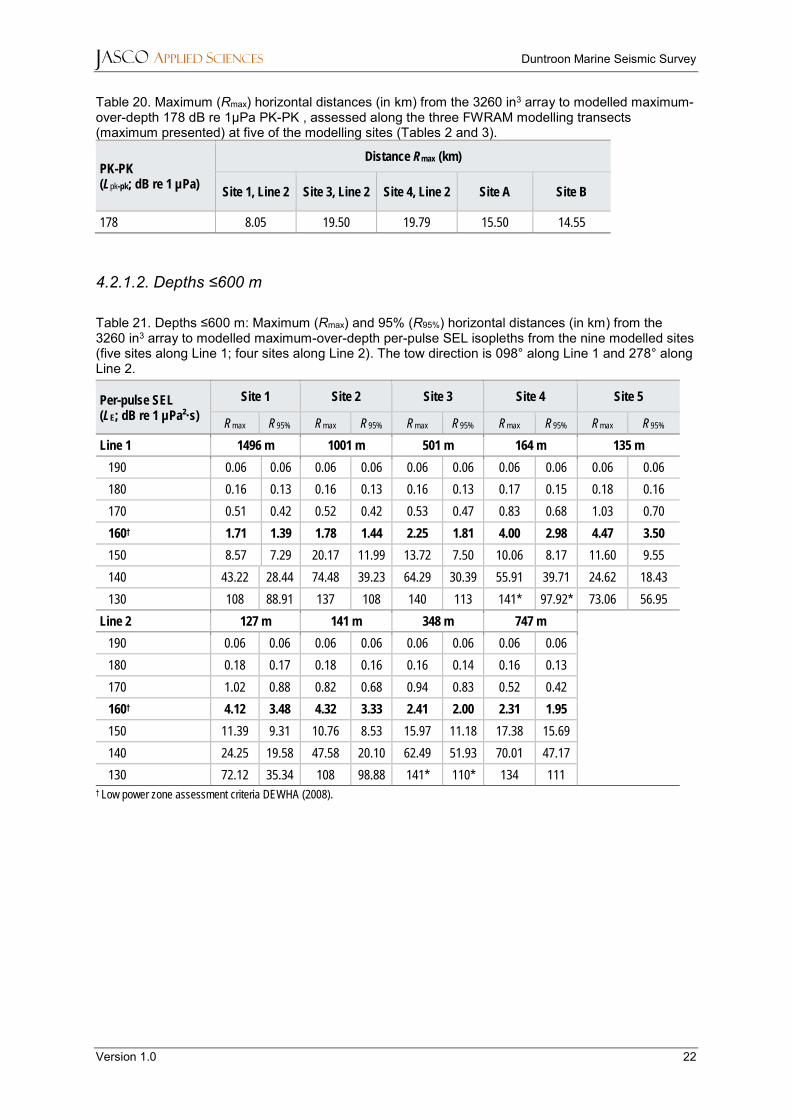
Table 20. Maximum (Rmax) horizontal distances (in km) from the 3260 in3 array to modelled maximum-over-depth 178 dB re 1µPa PK-PK ................................................................................. 22
Table 21. Depths ≤600 m: Maximum (Rmax) and 95% (R95%) horizontal distances (in km) from the 3260 in3 array to modelled maximum-over-depth per-pulse SEL isopleths from the nine modelled sites .................................................................................................................................. 22
Table 22. Depths ≤600 m: Maximum (Rmax) and 95% (R95%) horizontal distances (in km) from the 3260 in3 array to modelled maximum-over-depth SPL isopleths from the nine modelled sites ...... 23
Table 23. Depths ≤600 m: Maximum (Rmax) and 95% (R95%) horizontal distances (in km) from the 3260 in3 array to modelled maximum-over-depth SEL isopleths from the two modelled sites in 3-D Survey Area 2 ........................................................................................................................... 23
Table 24. Depths ≤600 m: Maximum (Rmax) and 95% (R95%) horizontal distances (in km) from the 3260 in3 array to modelled maximum-over-depth SPL isopleths from the two modelled sites in 3-D Survey Area 2 ........................................................................................................................... 24
Table 25. Maximum-over-depth SPL total ensonified area (km2): entire water column (EWC) and depths ≤600 m from the nine modelled sites ................................................................................... 24
Table 26. Difference in maximum-over-depth SPL ensonified area (km2) between entire water column and depths ≤600 m from the nine modelled sites ............................................................... 25
Table 27. Maximum-over-depth SPL total ensonified area (km2): entire water column (EWC) and depths ≤600 m from the two modelled sites in 3-D Survey Area 2. ................................................ 25
Table 28. Maximum (Rmax) horizontal distances (in m) from the 3260 in3 array to modelled seafloor PK from four transects ....................................................................................................... 25
Table 29. Maximum (Rmax) horizontal distances (in m) from the 3260 in3 array to modelled seafloor PK-PK for comparison to results in Payne et al. (2008), and Day et al. (2016a). ............. 26
Table 30. Maximum-over-depth results for frequency-weighted SEL 24 h PTS thresholds based on the NOAA Technical Guidance (NMFS 2018) over the entire water column. ............................ 59
Table 31. Results for SEL24h fish TTS criteria (LE,24h; 186 dB re 1 µPa²·s), for the entire water column (maximum-over-depth) and seafloor receptors. .................................................................. 59
Table 32. Received frequency-weighted SEL 24 h (LE,24h; dB re 1 µPa²·s) at five sampling locations. .......................................................................................................................................... 60
Table 33. Depths ≤600 m: Maximum-over-depth results for frequency-weighted SEL 24 h (LE,24h; dB re 1 µPa²·s) thresholds based on the NOAA Technical Guidance (NMFS 2018) for water depths ≤600 m. ................................................................................................................................ 60

JASCO APPLIED SCIENCES Duntroon Marine Seismic Survey
Version 1.0 vi
Table 34. Comparison (distance) between maximum (Rmax) and 95% (R95%) horizontal distances (in m) from the 3260 in3 array to modelled maximum-over-depth per-pulse SEL isopleths between sites at similar depths in 3-D Survey Area 1 and 2 (Tables 12 and 14). ........................... 70
Table 35. Summary of marine mammal PTS (injurious) onset distances. ............................................ 71 Table 36. Summary of marine mammal TTS onset distances .............................................................. 72

JASCO APPLIED SCIENCES Duntroon Marine Seismic Survey
Version 1.0 1
Executive Summary
Sound models were used to assess underwater noise levels during the proposed Duntroon Multi-Client Marine Seismic Survey (MSS) by PGS Australia. The modelling results are required for assessing the noise that marine fauna, are exposed to near survey operations. Previous modelling for this project assessed a 3090 in3 seismic airgun array (McPherson et al. 2017); however, a 3260 in3 is anticipated to be used in the survey and therefore is evaluated in this report. There is potential for the survey to be conducted any time during March – May or September – November; therefore, a review of sound speed profiles from these months versus May, which was used in the original modelling, was done to investigate the most conservative scenario, which was still found to be May. The modelling approach accounted for the acoustic emission characteristics of a 3260 in3 seismic airgun array that is likely to be operated during the survey and considered source directivity and the area’s range-dependent environmental properties relevant for the sound propagation.
The modelling study for the Duntroon MSS assessed twelve single pulse sites, nine of which were used to inform a representative accumulated sound exposure level (SEL, LE) scenario over 24 hours. Four sites additional sites relevant to seafloor peak pressure (PK, Lpk) and peak-to-peak pressure level (PK-PK, Lpk-pk) metrics were considered. Water depth for all sites varied from 127 to 1496 m.
The analysis considered the maximum distances away from the seismic source or survey lines at which several effects criteria were reached, with consideration of sound levels within Biological Areas of Importance for Australian sea lions and Southern Right Whales (SRW) north of the proposed survey area. Additionally, modelling considered the sound levels received by mysticetes (low-frequency cetaceans), and other fauna, such as turtles, which only utilise depths less than or equal to 600 m. A number of different criteria have been employed to assess the ranges for potential noise-induced effects to occur in each of the taxonomic groups, the results are summarised below for the representative single-impulse sites and accumulated SEL scenarios.
Marine Mammals
• NMFS (2018) marine mammal injury criteria: The results considered both metrics within the criteria for Permanent Threshold Shift (PTS) (PK and SEL24h). The farthest distance associated with either metric is required to be applied according to the criteria. Table 1 summarises the maximum distances and their associated metric. Because the array is not a point source (8.8 × 16.8 m), the actual ranges from the outer edge of the airgun array are small for mid-frequency cetaceans, and phocid and otariid pinnipeds.
• Based on the marine mammal injury criteria (NMFS 2018), temporary threshold shifts (TTS; non-injurious) are not predicted to occur in either in otariid pinnipeds, such as the Australian sea lion, or mid-frequency cetaceans, however they are predicted to occur in low and high-frequency cetaceans, along with phocid pinnipeds.
• United States National Marine Fisheries Service (NMFS; 2013) acoustic threshold for behavioural effects in marine mammals: Airgun sounds exceeded the sound pressure level (SPL) threshold of 160 dB re 1 µPa for behavioural effects on marine mammals within 7.6–13.05 km of the 3260 in3 seismic airgun array (Rmax distances) considering the entire water column or 6.59–13.05 km (Rmax distances) considering depths less than or equal to 600 m.
• Received sound levels at the boundary of the SRW calving and calving buffer BIAs were examined from the closest modelled site, and expressed in terms of unweighted and NMFS (2018) low-frequency (LF) weighted SPL. The LF weighted SPL is reported for comparison to the Wood et al. (2012) probabilistic disturbance threshold for migrating mysticetes, which have been demonstrated to respond to seismic airgun noise at lower received sound levels when compared to mysticetes in other behavioural states. The thresholds for migrating mysticetes are a 10% response likelihood at a weighted SPL of 120 dB re 1 µPa, 50% at a weighted SPL of 140 dB re 1 µPa, and a 90% response likelihood at a weighted SPL of 160 dB re 1 µPa.
o Unweighted sound levels at the boundaries of the calving buffer BIA and calving BIA are predicted to be 137 dB and 125 re 1 µPa (SPL), respectively.
o LF-weighted sound levels at the boundaries of the calving buffer BIA and calving BIA are predicted to be 132.8 dB and 121.8 re 1 µPa (SPL), respectively.

JASCO APPLIED SCIENCES Duntroon Marine Seismic Survey
Version 1.0 2
Table 1. Summary of marine mammal Permanent Threshold Shift (PTS) (injurious) onset distances, maximum of PK (Lpk) and SEL24h (LE) presented. The per-pulse modelling resolution was 20 m.
Relevant hearing group Metric associated with PTS onset Distance Rmax (m)
Low-frequency cetaceans† Weighted SEL24h (LE, 24h) 760
Mid-frequency cetaceans PK (Lpk) <20
High-frequency cetaceans PK (Lpk) 450
Phocid pinnipeds in water PK (Lpk) 40
Otariid pinnipeds in water PK (Lpk) <20
†The model does not account for shutdowns.
Turtle Behaviour
• United States NMFS criterion for behavioural effects in turtles: Airgun sounds exceeded the 166 dB re 1 µPa (SPL) threshold for behavioural effects within 1.9 to 4.32 km based on R95% distances, or 2.25 to 5.38 km based on Rmax distances at depths ≤600 m.
Fish, Turtle Injury, Fish Eggs, and Fish Larvae
• Based on PK metrics, acoustic injury (including both lethal and recoverable injuries) could be sustained at the seafloor within a maximum horizontal distance of 28 m of the seismic array for fish without a swim bladder (Site F, 160 m deep) and within a maximum horizontal distance of 150 m for fish with a swim bladder, turtles, fish eggs, and fish larvae (Site F, 160 m deep). The ranges associated with both possible mortality and potential mortal injury, and recoverable injury on fish, turtles, fish eggs and larvae suggested by Popper et al. (2014) using the SEL24h metric were not reached. Therefore, following the criteria, the PK metric should be used to assess these impacts to fish, turtles, fish eggs, and fish larvae.
Crustaceans, Bivalves, Plankton, Corals and Sponges
• To assist with the assessment of potential effects on crustaceans and bivalves, seafloor PK-PK was assessed at four locations, considering isopleths equivalent to those reported in Day et al. (2016b), along with the distance to a PK-PK of 202 dB re 1 µPa from Payne et al. (2007). The maximum distance to this sound level (202 dB re 1 µPa) is 718 m.
• To assist with the assessment of potential effects on plankton through comparison to relevant literature, the distance to the sound level of 178 dB re 1 µPa PK-PK from McCauley et al. (2017) was determined at five modelling sites through full-waveform modelling using FWRAM, and ranged from 8.1 to 19.8 km based on Rmax distances and maximum-over-depth.

JASCO APPLIED SCIENCES Duntroon Marine Seismic Survey
Version 1.0 3
1. Introduction
JASCO Applied Sciences (JASCO) performed a numerical estimation study of underwater sound levels associated with the Duntroon Multi-Client (MC) Marine Seismic Survey (MSS) proposed by Petroleum Geo-services (PGS) Australia in the Great Australian Bight (GAB). Previous modelling for this project assessed a 3090 in3 seismic airgun array (McPherson et al. 2017); however, a 3260 in3 is anticipated to be used in the survey and therefore is evaluated in this report. The modelling study specifically focused on one of the proposed three-dimensional (3-D) components of the survey, due to the acquisition line spacing and proximity to the coast and Kangaroo Island. The acoustic modelling evaluated the propagation of sounds produced by the seismic survey on marine fauna including cetaceans, pinnipeds, turtles, fish and invertebrates. The modelling considers a 3260 in3 airgun array towed at 7 m depth. Sound levels due to pressure are presented as sound pressure levels (SPL, Lp), zero-to-peak pressure levels (PK, Lpk), peak-to-peak pressure levels (PK-PK; Lpk-pk), and either single-impulse (i.e., per-pulse) or accumulated sound exposure levels (SEL, LE) as appropriate.
Per-pulse sound fields were modelled at:
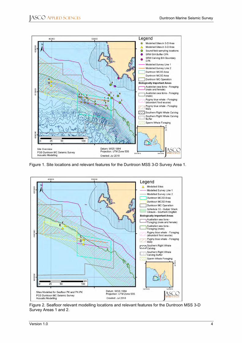
• Ten sites along two possible survey lines in in 3-D Survey Area 1 (Figure 1, Table 2)
• Two sites in in 3-D Survey Area 2 (Figure 1, Table 3)
• Four sites relevant to seafloor PK and PK-PK metrics (Figure 2, Table 7)
The modelling used seismic lines that were based on an acquisition pattern being considered for the proposed 3-D survey component that PGS provided to JASCO. This pattern was based on the original Bight Lightning MSS design, and was in a similar location to 3-D Survey Area 1. The model considers 24 hours of operation within this survey design. The acquired seismic lines are orientated with respect to prevailing weather conditions in the Great Australian Bight and are within an area that might best represent a 3-D acquisition area. These survey lines were selected because they best represent the range of bathymetry within the operational area closest to the Australian sea lion Biologically Important Areas (BIAs), and include the closest line to the Southern Right Whale (SRW) calving BIAs. The single impulse points within the Scenario are all those listed in Table 2.
To provided context for the received levels within the male and female sea lion foraging BIA which is not traversed by the vessel during the survey design, JASCO selected five locations to sample the modelled 24 h sound field. They represent the closest approach of the array to the BIA in broadside and endfire directions, or simply the closest in absolute terms, and the closest approach to the 100 m contour in either broadside direction or absolute terms. Tables 2–5 list the geographic coordinates of the modelled sites, survey lines, and sound field sampling locations.
Additionally, PGS requested that two per-pulse sites be modelled within a possible second 3-D survey area (3-D Survey Area 2) within the Duntroon MC MSS Operational area (Figure 1, Table 3). The footprints at these sites are compared to similar per-pulse sites within 3-D Survey Area 1. Additionally to assess the closest operational point to the Southern Right Whale (SRW) BIAs for calving and the calving buffer two locations were defined (Table 6), the sound levels from the closest operational point within 3-D Survey Area 1 (Line 2, Site 5) were predicted. PK and PK-PK at the seafloor were predicted at two sites within each 3-D survey area (Figure 2, Table 7).
Blue whales are known to primarily migrate and feed in the first few hundred metres of the water column (Croll et al. 2001, Goldbogen et al. 2011), with the deepest dive being reported from a pygmy blue whale being 506 m (Owen et al. 2016). Therefore, the sound levels received by mysticetes (low-frequency cetaceans), and other fauna which only utilise depths less than or equal to 600 m, such as turtles, have also been examined.
JASCO APPLIED SCIENCES Duntroon Marine Seismic Survey
Version 1.0 4
Figure 1. Site locations and relevant features for the Duntroon MSS 3-D Survey Area 1.
Figure 2. Seafloor relevant modelling locations and relevant features for the Duntroon MSS 3-D Survey Areas 1 and 2.

JASCO APPLIED SCIENCES Duntroon Marine Seismic Survey
Version 1.0 5
Table 2. Location of modelled sites on potential 3-D acquisition lines in 3-D Survey Area 1 of the Duntroon 3-D MSS (UTM zone 53S).
Line # Site # Latitude Longitude Easting Northing Water depth (m) Tow heading (°)
1
1 −35.4538 134.6535 468557 6076572 1496 098
2 −35.4655 134.7511 477418 6075302 1001 098
3 −35.4753 134.8331 484860 6074235 501 098
4 −35.4966 135.0135 501229 6071887 164 098
5 −35.5282 135.2866 525981 6068338 135 098
2
1 −35.4225 135.2578 523405 6080073 127 278
2 −35.3693 134.8035 482152 6085988 141 278
3 −35.3521 134.6603 469133 6087855 348 278
4 −35.3456 134.6064 464232 6088557 747 278
5 −35.4329 134.3488 531656 6078890 128 278
Table 3. Location details for modelled sites in 3-D Survey Area 2 of the Duntroon 3-D MSS (UTM zone 53S).
Site Latitude Longitude Easting Northing Water depth (m) Tow heading (°)
A −35.0171 133.8879 398537 6124501 496 278
B −35.0980 133.8903 398858 6115531 950 278
Table 4. Location details for the survey lines modelled in 3-D Survey Area 1 to assess the defined 24 h SEL scenario for the Duntroon 3-D MSS (UTM zone 53S).
Line # Position Latitude Longitude Easting Northing Tow heading (°)
1 Start −35.4424 134.5590 459976 6077803
098 End −35.5353 135.3488 531618 6067530
2 Start −35.4329 135.3488 531656 6078890
278 End −35.3399 134.5592 459940 6089173

JASCO APPLIED SCIENCES Duntroon Marine Seismic Survey
Version 1.0 6
Table 5. Location details for the 24 h sound field sampling locations for the Duntroon MSS operating in 3-D Survey Area 1 (UTM zone 53S).
Location Latitude Longitude Easting Northing Distance from closest
survey line (km)
1 Closest point between the array and the foraging (male and female)
sea lion BIA −35.3692 135.4365 539649 6085927 10.65
2 Closest point between the broadside of the array and the foraging (male
and female) sea lion BIA −35.3075 135.3703 533662 6092788 14.05
3 Closest point between the endfire of the array and the foraging (male and
female) sea lion BIA −35.4668 135.6470 558700 6074991 27.33
4 Closest point between the array and the 100 m isobath
−35.3262 135.5985 554397 6090622 25.60
5 Closest point between the broadside of the array and the 100 m isobath
−35.0958 135.4054 536948 6116257 37.75
Table 6. Location details for the SRW BIA relevant sound field sampling locations for the closest operation point from the Duntroon MSS operating in 3-D Survey Area 1 (UTM zone 53S).
Location Latitude Longitude Easting Northing
Boundary of SRW Calving Buffer BIA −35.1263 135.5173 547130.8 6112826
Boundary of SRW Calving BIA −34.955 135.6082 555533.2 6131782
Table 7. Location details for the Duntroon MSS modelled sites for seafloor PK and PK-PK metrics (UTM zone 53S).
Site Site label Latitude Longitude Easting Northing Water depth (m) Tow heading (°)
3-D Survey Area 1, Site 1 C −35.3675 134.7265 475159 6086162 200 098
3-D Survey Area 1, Site 2 D −35.4565 134.7216 474738 6076294 1099 098
3-D Survey Area 2, Site 1 E −35.1267 134.2016 427252 6112615 649 098
3-D Survey Area 2, Site 2 F −35.0786 134.2650 432994 6117992 160 098

JASCO APPLIED SCIENCES Duntroon Marine Seismic Survey
Version 1.0 7
2. Noise Effect Criteria
The perceived loudness of sound, especially impulsive noise such as from seismic airguns, is not generally proportional to the instantaneous acoustic pressure. Rather, perceived loudness depends on the time over which the pulse rises, how long this occurs for, and its frequency content. Thus, several sound level metrics are commonly used to evaluate noise and its effects on marine life (Appendix A). The period of accumulation associated with SEL is defined, with this report referencing either a “per pulse” assessment or over 24 h. Appropriate subscripts indicate any applied frequency weighting; unweighted SEL is defined as required. The acoustic metrics in this report reflect the updated ANSI and ISO standards for acoustic terminology, ANSI-ASA S1.1 (R2013) and ISO/DIS 18405.2:2017 (2016).
The noise criteria were chosen for this study include standard thresholds and thresholds suggested by the best available science (Sections 2.1–2.2 and Appendix A), additionally specific sound levels have been included for comparison to those reported in specific recent literature. All criteria and specific sound levels considered are as follows:
1. Peak pressure levels (PK; Lpk) and frequency-weighted accumulated sound exposure levels (SEL; LE,24h) from the U.S. National Oceanic and Atmospheric Administration (NOAA) Technical Guidance (NMFS 2018) for the onset of permanent threshold shift (PTS) and temporary threshold shift (TTS) in marine mammals.
a. TTS for low-frequency cetaceans is presented also considering the maximum-over-depth value for depths ≤600 m.
2. Marine mammal behavioural threshold based on the current interim U.S. National Marine Fisheries Service (NMFS) criterion (NMFS 2013) for marine mammals of 160 dB re 1 µPa SPL (Lp) for impulsive sound sources. Reported as both:
a. Maximum-over-depth value for entire water column
b. Maximum-over-depth value for depths ≤600 m.
3. Low-frequency (LF) weighted SPL for comparison to the Wood et al. (2012) probabilistic disturbance thresholds for migrating mysticetes (relevant for calving mysticetes), assessed using the NMFS (2018) frequency weighting function. The relevant thresholds are LF-weighted SPLs of 120, 140 and 160 dB re 1 µPa, relating to response likelihoods of 10, 50 and 90%, respectively. These thresholds are considered only at the closest modelling site to the SRW calving and calving buffer BIAs.
4. Sound exposure guidelines for fish, fish eggs and larvae, and turtles (Popper et al. 2014).
5. Threshold for turtle behavioural response of 166 dB re 1 μPa SPL (Lp) (NSF 2011), as applied by the US NMFS.
a. Maximum-over-depth value for entire water column
b. Maximum-over-depth value for depths ≤600 m.
6. PK-PK (Lpk-pk) at the seafloor is reported for comparison to results in Payne et al. (2008), and Day et al. (2016a).
7. 178 dB re 1 μPa PK-PK in the water column, reported for comparison to McCauley et al. (2017) for plankton.
Additionally, to assess the size of the low-power zone required under the Australian Environment Protection and Biodiversity Conservation (EPBC) Act Policy Statement 2.1, Department of the Environment, Water, Heritage and the Arts (DEWHA) (2008), the distance to an unweighted per-pulse SEL of 160 dB re 1 μPa2·s is reported as both:
a. Maximum-over-depth value for entire water column
b. Maximum-over-depth value for depths ≤600 m.

JASCO APPLIED SCIENCES Duntroon Marine Seismic Survey
Version 1.0 8
2.1. Marine Mammals
The criteria applied in this study to assess possible effects of airgun noise on marine mammals are summarised in Table 8 and detailed in Sections 2.1.2 and 2.1.3, with frequency weighting explained in Section 2.1.1 and Appendix A.2.
Table 8. The SPL (unweighted, Lp, and LF-weighted, Lp, LF) SEL24h (LE,24h) and PK (Lpk) thresholds for acoustic effects on marine mammals. Injury is defined as permanent threshold shift (PTS).
Hearing group
Behaviour
NMFS (2018)
PTS onset thresholds* (received level)
TTS onset thresholds* (received level)
SPL (dB re 1 μPa)
Weighted SEL24h (LE, 24;
dB re 1 μPa2·s)
PK (Lpk; dB re 1 μPa)
Weighted SEL24h (LE, 24;
dB re 1 μPa2·s)
PK (Lpk; dB re 1 μPa)
Low-frequency cetaceans
160 (Lp) (NMFS 2013)
183 219 168 213
Mid-frequency cetaceans
185 230 170 224
High-frequency cetaceans
155 202 140 196
Phocid pinnipeds in water
185 218 170 226
Otariid pinnipeds in water
203 232 188 212
Migrating and calving SRW
Modified Wood et al. (2012) – See
Table 9 Refer to Low-frequency cetaceans
* Dual metric acoustic thresholds for impulsive sounds: Use whichever results in the largest isopleth for calculating PTS onset. If a non-impulsive sound has the potential of exceeding the peak sound pressure level thresholds associated with impulsive sounds, these thresholds should also be considered. Lpk, flat–peak sound pressure is flat weighted or unweighted and has a reference value of 1 µPa LE - denotes cumulative sound exposure over a 24-hour period and has a reference value of 1 µPa2s Subscripts indicate the designated marine mammal auditory weighting.
2.1.1. Marine mammal weighting functions The potential for anthropogenic sounds to impact marine mammals is largely dependent on whether the sound occurs at frequencies that an animal can hear well, unless the sound pressure level is so high that it can cause physical tissue damage regardless of frequency. Auditory (frequency) weighting functions reflect an animal’s ability to hear a sound (Nedwell and Turnpenny 1998, Nedwell et al. 2007). Auditory weighting functions have been proposed for marine mammals, specifically associated with PTS thresholds expressed in metrics that consider what is known about marine mammal hearing (e.g., SEL (LE)) (Southall et al. 2007, Erbe et al. 2016, Finneran 2016). Marine mammal auditory weighting functions published by Finneran (2016) are included in the NMFS 2018 Technical Guidance for use in conjunction with corresponding PTS (injury) onset acoustic criteria.
The application of marine mammal auditory weighting functions emphasises the importance of making measurements and characterising sound sources in terms of their overlap with biologically-important frequencies (e.g., frequencies used for environmental awareness, communication or the detection of predators or prey), and not only the frequencies of interest or concern for the completion of the sound-producing activity (i.e., context of sound source; NMFS 2018).

JASCO APPLIED SCIENCES Duntroon Marine Seismic Survey
Version 1.0 9
2.1.2. Behavioural response Numerous studies on marine mammal behavioural responses to sound exposure have not resulted in consensus in the scientific community regarding the appropriate metric for assessing behavioural reactions. However, it is recognised that the context in which the sound is received affects the nature and extent of responses to a stimulus (Southall et al. 2007, Ellison and Frankel 2012, Southall et al. 2016). Because of the complexity and variability of marine mammal behavioural responses to acoustic exposure, NMFS has not yet released technical guidance on behaviour thresholds for use in calculating animal exposures (NMFS 2018). The NMFS currently uses a step function to assess behavioural impact. A 50% probability of inducing behavioural responses at a SPL of 160 dB re 1 µPa was derived from the HESS (1999) report which, in turn, was based on the responses of migrating mysticete whales to airgun sounds (Malme et al. 1983, Malme et al. 1984). The HESS team recognized that behavioural responses to sound may occur at lower levels, but significant responses were only likely to occur above a SPL of 140 dB re 1 µPa. An extensive review of behavioural responses to sound was undertaken by Southall et al. (2007, their Appendix B). Southall et al. (2007) found varying responses for most marine mammals between a SPL of 140 and 180 dB re 1 µPa, consistent with the HESS (1999) report, but lack of convergence in the data prevented them from suggesting explicit step functions. Absence of controls, precise measurements, appropriate metrics, and context dependency of responses (including the activity state of the animal) all contribute to variability. Therefore, unless otherwise specified, the relatively simple sound level criterion for potentially disturbing a marine mammal applied by NMFS has been used. For impulsive sounds, this threshold is 160 dB re 1 µPa SPL for cetaceans (NMFS 2013).
Wood et al. (2012) proposed a graded probability of response for impulsive sounds using a frequency weighted SPL metric. They defined behavioural response categories for sensitive species (including harbor porpoise and beaked whales) and for migrating mysticetes. The migrating mysticete category has been applied in this analysis to Southern Right Whales, in particular within the calving and calving buffer BIAs, but also during migration, to assess behavioural response to impulsive sounds (Table 9). The Wood et al. (2012) approach has been updated to consider the frequency weighting from NMFS (2018).
Table 9. Behavioural exposure criteria used in this analysis for calving and migrating SRW Probability of behavioural response frequency-weighted sound pressure level (SPL dB re 1 µPa). Probabilities are not additive. Adapted from Wood et al. (2012).
Probability of response to frequency-weighted SPL (dB re 1 µPa)
120 140 160
10% 50% 90%
2.1.3. Injury and hearing sensitivity changes There are two categories of auditory threshold shifts or hearing loss: permanent threshold shift (PTS), a physical injury to an animal’s hearing organs and Temporary Threshold Shift (TTS), a temporary reduction in an animal’s hearing sensitivity as the result of receptor hair cells in the cochlea becoming fatigued.
To assist in assessing the potential for injuries to marine mammals this report applies the criteria recommended by NMFS (2018), considering both PTS and TTS, to help assess the potential for injuries to marine mammals. Appendix A provides more information about the NMFS (2018) criteria.
2.2. Fish, Turtles, Fish Eggs, and Fish Larvae
In 2006, the Working Group on the Effects of Sound on Fish and Turtles was formed to continue developing noise exposure criteria for fish and turtles, work begun by a NOAA panel two years earlier. The resulting guidelines included specific thresholds for different levels of effects and for different

JASCO APPLIED SCIENCES Duntroon Marine Seismic Survey
Version 1.0 10
groups of species (Popper et al. 2014). These guidelines defined quantitative thresholds for three types of immediate effects:
• Mortality, including injury leading to death.
• Recoverable injury, including injuries unlikely to result in mortality, such as hair cell damage and minor haematoma.
• TTS
Masking and behavioural effects were assessed by Popper et al (2014) only qualitatively, by assessing relative risk rather than by specific sound level thresholds. These effects are not assessed in this report. Because the presence or absence of a swim bladder and ancilliary structures has a role in hearing in fish, their susceptibility to hearing related injury from noise exposure varies depending on the species and anatomy. Accordingly, , Popper et al (2014) suggested different thresholds for fish without a swim bladder (also appropriate for sharks and applied to whale sharks in the absence of other information), fish with a swim bladder not used for hearing, and fish that use their swim bladders for hearing. Turtles, fish eggs, and fish larvae were considered separately.
Table 10 lists relevant effect thresholds suggested by Popper et al. (2014). In general, any adverse effects of seismic sound on fish behaviour depends on the species, the state of the individuals exposed, and other factors. Despite mortality being a possible outcome for fish exposed to airgun sounds, Popper et al. (2014) do not reference this effect occurring, but since that time, newer studies have further examined that question. Popper et al. (2016) added further information to the possible levels of impulsive seismic airgun sound to which adult fish can be exposed without immediate mortality. They found that the two fish species in their study, with individual body masses in the range 200–400 g, exposed to a maximum received level of either 231 dB re 1 μPa (PK) or 205 dB re 1 μPa2∙s (per-pulse SEL), remained alive for 7 days after exposure and that the probability of mortal injury did not differ between exposed and control fish.
The SEL metric integrates noise intensity over some period of exposure. Because the period of integration for regulatory assessments is not well defined for sounds that do not have a clear start or end time, or for very long-lasting exposures, a period of time must be defined. For marine mammals, following the Southall et al. (2007) criteria, the period is 24 h or the duration of the activity, whichever is shorter. Popper et al. (2014) recommended a standard period of time should be applied, where this is either defined as a justified fixed period or the duration of the activity, however they also included caveats about the length of time to which fish could be exposed because fish and sources can move or remain stationary. When Popper et al. (2014) discuss their criteria, they refer to complications determining a relevant period for mobile seismic surveys and mobile or site-attached fish, because the received levels at the fish change between impulses due to the mobile source, and that in reality a revised guideline based on the closest PK or the per-pulse SEL might be more useful than one based on accumulated SEL. This is because exposures at the closest point of approach are the primary contributors to a receiver’s accumulated level (Gedamke et al. 2011). Additionally, several important factors determine the likelihood and duration a receiver is expected to be very close to a sound source (i.e., overlap in space and time between the source and receiver). For example, accumulation time for mobile sources moving fast relative to the receiver is driven primarily by the source’s characteristics (i.e., speed, duty cycle) (NMFS 2018).
Popper et al. (2014) summarise that in all TTS studies considered, fish that showed TTS recovered to normal hearing levels within 18–24 hours. Due to this, a period of accumulation of 24 h has been applied in this study for SEL, which is similar to that applied for marine mammals in Southall et al. (2007) and NMFS (2018).

JASCO APPLIED SCIENCES Duntroon Marine Seismic Survey
Version 1.0 11
Table 10. Criteria for seismic noise exposure for fish and turtles, adapted from Popper et al. (2014).
Type of animal Mortality and
Potential mortal injury
Impairment Behaviour
Recoverable injury TTS Masking
Fish: No swim bladder (particle motion detection)
> 219 dB SEL24h or
> 213 dB PK
> 216 dB SEL24h or
> 213 dB PK >> 186 dB SEL24h
(N) Low (I) Low (F) Low
(N) High (I) Moderate
(F) Low
Fish: Swim bladder not involved in hearing (particle motion detection)
210 dB SEL24h or
> 207 dB PK
203 dB SEL24h or
> 207 dB PK >> 186 dB SEL24h
(N) Low (I) Low (F) Low
(N) High (I) Moderate
(F) Low
Fish: Swim bladder involved in hearing (primarily pressure detection)
207 dB SEL24h or
> 207 dB PK
203 dB SEL24h or
> 207 dB PK 186 dB SEL24h
(N) Low (I) Low
(F) Moderate
(N) High (I) High
(F) Moderate
Turtles 210 dB SEL24h
or > 207 dB PK
(N) High (I) Low (F) Low
(N) High (I) Low (F) Low
(N) Low (I) Low (F) Low
(N) High (I) Moderate
(F) Low
Fish eggs and fish larvae > 210 dB SEL24h
or > 207 dB PK
(N) Moderate (I) Low (F) Low
(N) Moderate (I) Low (F) Low
(N) Low (I) Low (F) Low
(N) Moderate (I) Low (F) Low
Notes: Peak sound level (PK) dB re 1 µPa; SEL24h dB re 1µPa2∙s. All criteria are presented as sound pressure, even for fish without swim bladders, since no data for particle motion exist. Relative risk (high, moderate, or low) is given for animals at three distances from the source defined in relative terms as near (N), intermediate (I), and far (F).
Turtle Behavioural Response There is a paucity of data regarding responses of turtles to acoustic exposure, and no studies of hearing loss due to exposure to loud sounds. McCauley et al. (2000) observed the behavioural response of caged turtles—green (Chelonia mydas) and loggerhead (Caretta caretta)—to an approaching seismic airgun. For received levels above 166 dB re 1 μPa (SPL), the turtles increased their swimming activity and above 175 dB re 1 μPa they began to behave erratically, which was interpreted as an agitated state. The 166 dB re 1 μPa level has been used as the threshold level for a behavioural disturbance response by NMFS and applied in the Arctic Programmatic Environment Impact Statement (PEIS) (NSF 2011). At that time, and in the absence of any data from which to determine the sound levels that could injure an animal, TTS or PTS onset were considered possible at an SPL of 180 dB re 1 μPa (NSF 2011). Some additional data suggest that behavioural responses occur closer to an SPL of 175 dB re 1 μPa, and TTS or PTS at even higher levels (Moein et al. 1995), but the received levels were unknown and the NSF (2011) PEIS maintained the earlier NMFS criteria levels of 166 and 180 dB re 1 μPa (SPL) for behavioural response and injury, respectively. Popper et al. (2014) suggested injury to turtles could occur for sound exposures above 207 dB re 1 μPa (PK) or above 210 dB re 1 μPa2·s (SEL24h) (Table 10). Sound levels defined by Popper et al. (2014) show that animals are very likely to exhibit a behavioural response when they are near an airgun (tens of metres), a moderate response if they encounter the source at intermediate ranges (hundreds of metres), and a low response if they are far (thousands of meters) from the airgun. Both the NMFS criteria for behavioural disturbance (SPL of 166 dB re 1 μPa) and the Popper et al. (2014) injury criteria were included in this analysis, although the analysis did not consider the ranges at which an animal could suffer impairment, as defined by Popper et al. (2014).

JASCO APPLIED SCIENCES Duntroon Marine Seismic Survey
Version 1.0 12
3. Methods
This section details the methodology for predicting source levels, modelling sound propagation, and assessing distances to the selected impact criteria.
3.1. Acoustic Source Model
The source levels and directivity of the airgun array were predicted with JASCO’s Airgun Array Source Model (AASM), which accounts for:
• Array layout
• Volume, tow depth, and firing pressure of each airgun
• Interactions between different airguns in the array
The array was modelled over AASM’s full frequency range, up to 25 kHz. Details of the model are described in Appendix B.
3.2. Sound Propagation Models
Four sound propagation models (Appendix C) were used to predict the acoustic field around the airgun array for frequencies from 5 Hz to 25 kHz:
• Range-dependent parabolic equation model (Marine Operations Noise Model, MONM)
• Range-dependent ray tracing model (BELLHOP)
• Full Waveform Range-dependent Acoustic Model (FWRAM)
• Wavenumber integration model (VSTACK).
The models were used in combination to characterise the acoustic fields at short and long ranges in terms of SEL, SPL, PK, and PK-PK.
3.3. Parameter Overview
The specifications of the airgun array source modelled at all sites and the environmental parameters used in the propagation models are described in detail in Appendix D.
The airgun array under consideration for the proposed Duntroon MSS is a 8.8 × 16.8 m 3260 in3 seismic array consisting of two strings towed at a depth of 7 m, Figure D-4, Table D-2. The firing pressure will be 2000 psi.
A single sound speed profile that provided the greatest propagation across the period January to May and September to November was applied, which occurs during the month of May.

JASCO APPLIED SCIENCES Duntroon Marine Seismic Survey
Version 1.0 13
3.4. Accumulated SEL
Method overview During a seismic survey, a new portion of sound energy is introduced into the environment with each pulse from the airgun array. While some impact criteria are based on per-pulse energy released, others, such as the marine mammal SEL criteria used in this report (Section 2.1) consider the total acoustic energy marine fauna is subjected to over 24 hours. An accurate assessment of the cumulative acoustic field depends not only on the parameters of each impulse, but also on the number of impulses delivered over a period and the relative position of the impulses.
When there are many seismic pulses, it becomes computationally prohibitive to perform sound propagation modelling for every single event. The offset between the consecutive seismic impulses is small enough, however, that the environmental parameters that influence sound propagation are virtually the same for many impulse points. The acoustic fields can, therefore, be modelled for a subset of seismic pulses and estimated at several adjacent ones. After sound fields from representative impulse locations are calculated, they are adjusted to account for the source position for nearby impulses.
Although estimating the cumulative sound field with the described approach is not as precise as modelling sound propagation at every impulse location, small-scale, site-specific sound propagation features tend to blur and become less relevant when sound fields from adjacent impulses are summed. Larger scale sound propagation features, primarily dependent on water depth, dominate the cumulative field. The accuracy of the present method acceptably reflects those large-scale features, thus providing a meaningful estimate of a wide area SEL field in a computationally feasible framework.
Scenario definition Because modelling the thousands of impulses needed to represent 24 hours of seismic operation is time consuming, we estimated the acoustic fields based on nine per-pulse model sites from representative source locations; these formed the library of representative footprints. The survey lines within the 24-hour exposure calculation were segmented into zones by classifying impulse points into one of nine representative sites based on geographic similarity (Figure 3). One scenario, which represents possible methods for acquisition because the design is not yet finalised, was defined to assess accumulated SEL over 24 hours of seismic operation along the supplied survey lines.
To produce maps of cumulative received sound level distribution and calculate distances to specified maximum over depth sound level thresholds, the sound level was calculated at a subset of points within the modelled region. The radial grids of sound levels of the modelled sites at each point were then resampled (by linear triangulation) to produce a regular Cartesian grid. These grids were transposed geographically to each impulse location along the survey lines, based on similar water depths at the modelled location and at the impulse location. The sound field grids from all impulses were summed, using Equation A-6, to produce the cumulative sound field grid. The produced grids had a cell size of 50 m. The contours and threshold ranges were calculated from these flat Cartesian projections of the modelled acoustic fields.
We postulated a scenario in which the vessel travelled along Lines 1 and 2 (Figure 1) over 24 hr at a speed of 7.78 km/h (4.2 knots), which conforms to the PGS specifications of an impulse every 16.67 m. The model estimated 8681 seismic events occurred over this period. This period conforms with the requirements of the NMFS (2018) criteria, and is considered sufficient to assess the accumulated sound fields in relation to the adjacent BIAs. The resulting ranges to the relevant thresholds equal the maximum range calculated over 24 hours.

JASCO APPLIED SCIENCES Duntroon Marine Seismic Survey
Version 1.0 14
Figure 3. Overview of zones along the modelled survey lines represented by the nine modelled sites.
3.5. Geometry and Modelled Regions
The sound fields were modelled using MONM and BELLHOP models up to distances of 100 km from the source, with a 20 m horizontal separation between receiver points along the modelled radials. Sound fields were modelled with a horizontal angular resolution of = 2.5° for a total of N = 144 radial planes. Receiver depths were chosen to span the entire water column over the modelled areas, from 1 m to a maximum of 5000 m, depending upon the site, with step sizes increasing with depth.
JASCO APPLIED SCIENCES Duntroon Marine Seismic Survey
Version 1.0 15
Full waveform model FWRAM was run to a distance of 10 km, with a range step of 20 m, along three radials (each broadside and aft endfire directions) for computational efficiency. The model ran from 5 to 1024 Hz in 0.5 Hz steps to provide a 2 second time-domain window for pulse analysis. This was done to compute SEL-to-SPL conversion functions (Appendix D.2). FWRAM was also used to model the PK levels in the water column.
The nearfield full-waveform model VSTACK was used to model both seafloor PK and PK-PK levels. The maximum modelled range for VSTACK was 500 m. Because VSTACK assumes constant bathymetry, radials were only run in four directions (endfire: fore and aft; broadside: port and starboard). Received levels were computed for test receivers on the seafloor.

JASCO APPLIED SCIENCES Duntroon Marine Seismic Survey
Version 1.0 16
4. Results
This section presents the model results as distances to sound level thresholds and as sound field contour maps.
4.1. Acoustic Source Levels and Directivity
The pressure signatures of the individual airguns and the composite 1/3-octave-band point-source equivalent directional levels of the arrays were modelled with AASM (Section 3.1). Although AASM accounts for the effects of surface-reflected signals on bubble oscillations and inter-bubble interactions in the notional pressure signatures of each airgun, the signal reflected off the water surface (known as surface ghost) is not included in the far-field source signatures; however, the acoustic propagation models account for those surface reflections because they are a property of the propagating medium rather than the source.
The horizontal and vertical overpressure signatures, corresponding power spectrum levels, and the horizontal directivity plots for the array is provided in Appendix B.2.
To help compare these results to the outputs of other airgun array source models, Table 11 presents the vertical source level that accounts for the surface ghost, and lists the broadband PK, and per-pulse SEL source levels of the array in the endfire, broadside, and vertical directions.
Table 11. Source level specifications in the horizontal plane for the 3260 in3 array, for a 7 m tow depth. Source levels are for a point-like acoustic source with equivalent far-field acoustic output in the specified direction. Sound level metrics are per-pulse and unweighted.
Direction
Peak source pressure level
(LS,pk) (dB re 1 μPa2m2)
Per-pulse source SEL (LS,E) (dB 1 μPa2m2s)
10–2000 Hz 2000–25000 Hz 10–25000 Hz
Broadside 249.5 224.9 186.9 224.9
Endfire 246.2 223.5 186.9 223.5
Vertical (no ghost) 255.6 228.6 194.6 228.6
Vertical (with ghost) 255.6 231.1 197.5 231.1
4.2. Single Pulse Sound Fields
Single pulse sound fields were modelled at:
• Ten sites along two possible survey lines in in 3-D Survey Area 1 (Table 2).
• Two sites in in 3-D Survey Area 2 (Table 3).
• Four sites relevant to seafloor PK and PK-PK metrics (Table 7).
Distances to isopleths for maximum-over-depth per-pulse SEL and SPL are presented in Tables 12 and 14, and Tables 13 and 15 respectively. The maximum-over-depth LF-weighted SPL isopleths from Line 2 Site 5 are presented in Table 16. Table 17 presents distances to the PK thresholds based on the NOAA Technical Guidance (NMFS 2018). The SPL at the Neptune Islands and the SRW BIAs from the closest per-pulse modelled site are presented in Table 18, with LF-weighted SPLs at the boundaries of the SRW BIAs shown in Table 19.
To assist with the assessment of sound levels received by marine fauna in the upper 600 m of the water column, maximum-over-depth results, where the depth range is restricted to the upper 600 m, are presented for per-pulse SEL and SPL in Tables 21 and 23, Tables 22 and 24 respectively. The ensonified area for SPL footprints for both the entire water column and depths less than or equal to

JASCO APPLIED SCIENCES Duntroon Marine Seismic Survey
Version 1.0 17
600 m for the 170, 160, and 150 dB re 1 µPa isopleths are presented in Table 25 (3-D Survey Area 1) and Table 27 (3-D Survey Area 2), with differences provided in Table 26 for 3-D Survey Area 1. Distances to seafloor PK and PK-PK metrics were determined through considering the four broadside and endfire transects, and the results are presented in Tables 28 and 29.
Considering 3-D Survey Area 1, Figures 4–11 show example maps of maximum-over-depth sound level in per-pulse SEL and SPL for:
• A site in deep water (Site 1, Line 1),
• The site with the largest 160 dB re 1 µPa Rmax (Site 2, Line 1),
• A site on the continental shelf edge (Site 4, Line 1), and
• A site on the continental shelf (Site 1, Line 2).
Corresponding vertical slices of the estimated sound fields for per-pulse SEL and SPL are shown in Figures 18–23, which demonstrate the distribution of sound in the water column in the broadside and endfire directions. The sound fields in the offshore broadside direction at longer ranges are shown in a vertical slice of per-pulse SEL for Site 2, Line 1 (Figure 24), and SPL for Site 3, Line 2 (Figure 25).
Maps for the two additional modelling sites in 3-D Survey Area 2 are shown in Figures 12–15, with associated vertical slice plots in Figures 26–30. The sound fields in the offshore broadside direction at longer ranges are shown in a vertical slice of per-pulse SEL for Site A (Figure 31).
A map for an additional modelling site in the 3-D Survey Area 1 closest to the SRW BIAs (Site 5, Line 2) is shown in Figure 16. The map shows that the levels within the BIAs are below 140 dB re 1µPa, with levels at the BIA boundaries shown in Table 18. The LF-weighted SPL sound fields at this site are shown in Figure 17, with levels at the BIA boundaries shown in Table 19.
The decay of seafloor PK and PK-PK as the distance from the source increases are shown in Figures 38 and 39. These figures show the maximum predicted level from each of the four modelled transects, one in each of the broadside and endfire directions.

JASCO APPLIED SCIENCES Duntroon Marine Seismic Survey
Version 1.0 18
Tabulated Results
4.2.1.1. Entire water column
Table 12. Maximum (Rmax) and 95% (R95%) horizontal distances (in km) from the 3260 in3 array to modelled maximum-over-depth per-pulse SEL isopleths from the nine modelled single-shot sites (five sites along Line 1; four sites along Line 2). The tow direction is 098° along Line 1 and 278° along Line 2. The 160 dB re 1 µPa²·s isopleth (bold values) is associated with the DEWHA (2008) criterion.
Per-pulse SEL (LE; dB re 1 µPa²·s)
Site 1 Site 2 Site 3 Site 4 Site 5
Rmax R95% Rmax R95% Rmax R95% Rmax R95% Rmax R95%
Line 1 1496 m 1001 m 501 m 164 m 135 m
190 0.06 0.06 0.06 0.06 0.06 0.06 0.06 0.06 0.06 0.06
180 0.16 0.13 0.16 0.13 0.16 0.13 0.17 0.15 0.18 0.16
170 0.51 0.42 0.52 0.42 0.53 0.47 0.83 0.68 1.03 0.70
160† 1.75 1.54 3.20 2.52 2.88 2.29 4.00 2.98 4.47 3.50
150 9.12 7.26 20.17 11.86 13.94 10.75 10.06 8.16 11.60 9.55
140 43.51 31.95 74.48 47.52 88.48 69.88 60.16 47.22 24.62 18.43
130 108 91.81 137 109 141* 113* 141* 114* 91.24 64.35
Line 2 127 m 141 m 348 m 747 m
190 0.06 0.06 0.06 0.06 0.06 0.06 0.06 0.06
180 0.18 0.17 0.18 0.16 0.16 0.14 0.16 0.13
170 1.02 0.88 0.82 0.68 0.94 0.83 0.52 0.42
160† 4.12 3.48 4.32 3.33 2.51 2.06 3.18 2.45
150 11.39 9.31 10.76 8.53 15.97 11.33 17.38 15.54
140 24.25 19.58 47.58 32.48 101 64.30 70.47 47.84
130 72.12 39.52 122 104 141* 114* 137 113
* Radii extend beyond modelling boundary. † Low power zone assessment criteria DEWHA (2008).

JASCO APPLIED SCIENCES Duntroon Marine Seismic Survey
Version 1.0 19
Table 13. Maximum (Rmax) and 95% (R95%) horizontal distances (in km) from the 3260 in3 array to modelled maximum-over-depth SPL isopleths from the nine modelled single-shot sites (five sites along Line 1; and four sites along Line 2) The tow directions for Line 1 is 098° and 278° along Line 2.
SPL (Lp; dB re 1 µPa)
Site 1 Site 2 Site 3 Site 4 Site 5
Rmax R95% Rmax R95% Rmax R95% Rmax R95% Rmax R95%
Line 1 1496 m 1001 m 501 m 164 m 135 m
190 0.14 0.12 0.14 0.12 0.14 0.12 0.15 0.12 0.15 0.14
180 0.45 0.36 0.45 0.37 0.46 0.38 0.76 0.63 0.72 0.60
170 1.42 1.24 2.68 2.20 2.59 2.07 3.24 2.46 3.63 2.80
166† 4.45 3.57 4.43 3.46 3.58 2.82 4.89 3.81 5.38 4.32
160‡ 7.60 6.08 11.89 9.78 10.77 6.48 7.87 6.32 9.09 7.38
150 37.84 28.29 48.94 42.21 60.53 45.60 38.25 32.07 19.24 14.62
140 107 89.89 133 100 141* 114* 128 103 65.85 38.56
130 141* 116* 141* 116* 141* 118* 141* 115* 141* 109*
Line 2 127 m 141 m 348 m 747 m
190 0.16 0.14 0.15 0.14 0.14 0.12 0.14 0.12
180 0.73 0.61 0.72 0.60 0.84 0.44 0.45 0.37
170 3.61 2.86 3.59 2.82 2.28 1.80 2.75 2.11
166† 5.13 4.30 5.30 4.17 3.69 2.96 4.16 3.33
160‡ 8.71 7.16 8.71 6.81 11.05 6.67 12.75 6.25
150 20.36 16.32 33.92 20.63 59.16 42.25 54.60 43.47
140 43.02 34.41 106 94.12 141* 114* 132 108
130 114 92.61 141* 113* 141* 119* 141* 118*
* Radii extend beyond modelling boundary. † Threshold for turtle behavioural response to impulsive noise (NSF 2011). ‡ Marine mammal behavioural threshold for impulsive sound sources (NMFS 2013).
Table 14. Maximum (Rmax) and 95% (R95%) horizontal distances (in km) from the 3260 in3 array to modelled maximum-over-depth per-pulse SEL isopleths from the two modelled sites in 3-D Survey Area 2, and Line 2 Site 5 from 3-D Survey Area 2. (Tables 2 and 3).
Per-pulse SEL (LE; dB re 1 µPa²·s)
Site A 496 m depth
Site B 950 m depth
Line 2, Site 5
128 m depth
Rmax R95% Rmax R95% Rmax R95%
190 0.06 0.06 0.06 0.06 0.61 0.60
180 0.16 0.13 0.16 0.13 0.19 0.16
170 0.56 0.48 0.51 0.42 1.05 0.90
160† 2.78 2.23 3.03 2.52 4.11 3.50
150 13.86 12.36 11.83 9.43 21.37 16.53
140 69.07 49.64 48.69 37.85 40.82 33.79
130 128 106 106 90.22 106.52 89.39
† Low power zone assessment criteria DEWHA (2008).

JASCO APPLIED SCIENCES Duntroon Marine Seismic Survey
Version 1.0 20
Table 15. Maximum (Rmax) and 95% (R95%) horizontal distances (in km) from the 3260 in3 array to modelled maximum-over-depth SPL isopleths from the two modelled sites in 3-D Survey Area 2, and Line 2 Site 5 in 3-D Survey Area 2 (Tables 2 and 3).
SPL (Lp; dB re 1 µPa)
Site A 496 m depth
Site B 950 m depth
Line 2, Site 5
128 m depth
Rmax R95% Rmax R95% Rmax R95%
190 0.14 0.12 0.14 0.12 0.16 0.14
180 0.46 0.40 0.45 0.37 0.74 0.62
170 2.55 1.99 2.66 2.28 3.31 2.87
166† 4.00 3.31 3.84 3.17 5.03 4.25
160‡ 13.05 8.66 9.10 6.72 8.99 7.13
150 65.65 41.90 43.29 32.91 21.37 16.53
140 117 97.73 105 90.18 40.82 33.79
130 141* 119* 141* 119* 107 89.39
* Radii extend beyond modelling boundary. † Threshold for turtle behavioural response to impulsive noise (NSF 2011). ‡ Marine mammal behavioural threshold for impulsive sound sources (NMFS 2013).
Table 16. LF-weighted SPL: Maximum (Rmax) and 95% (R95%) horizontal distances (in km) from the 3260 in3 array to modelled maximum-over-depth LF-weighted SPL isopleths from Line 2 Site 5 in 3-D Survey Area 2 (Table 2).
LF-weighted SPL (Lp, LF; dB re 1 µPa)
Line 2, Site 5
128 m depth
Rmax R95%
190 0.08 0.07
180 0.49 0.45
170 1.95 1.61
160* 5.89 5.05
150 16.40 12.85
140‡ 34.80 27.92
130 99.30 58.01
120† 120.14 95.77 † 10% probability of response for migrating mysticetes, Wood et al. (2012). ‡ 50% probability of response for migrating mysticetes, Wood et al. (2012). * 90% probability of response for migrating mysticetes, Wood et al. (2012).
JASCO APPLIED SCIENCES Duntroon Marine Seismic Survey
Version 1.0 21
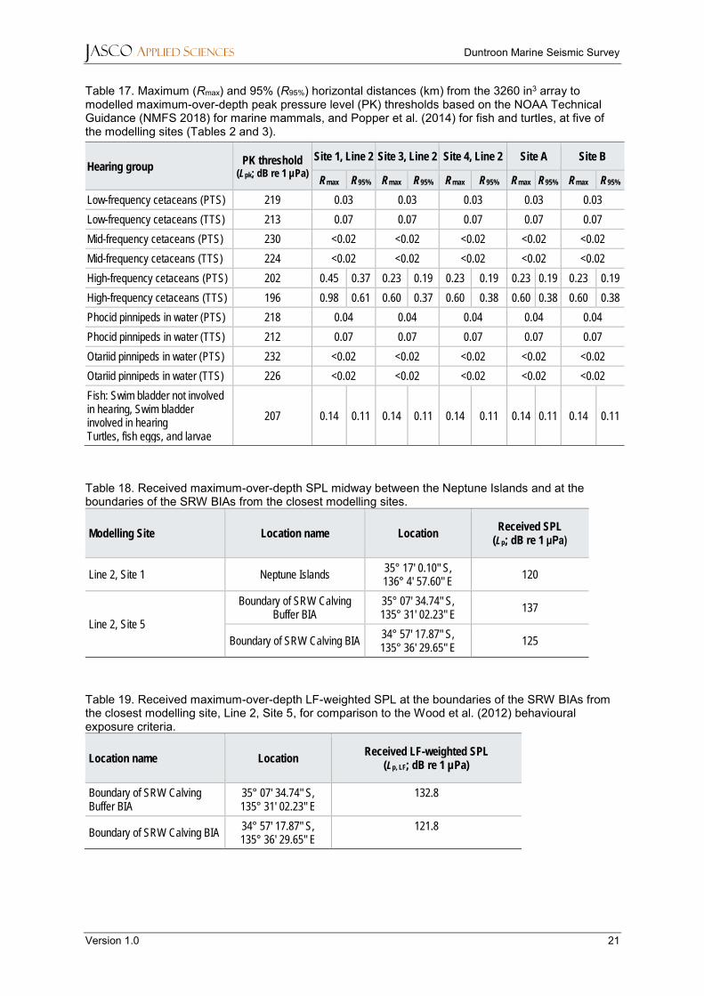
Table 17. Maximum (Rmax) and 95% (R95%) horizontal distances (km) from the 3260 in3 array to modelled maximum-over-depth peak pressure level (PK) thresholds based on the NOAA Technical Guidance (NMFS 2018) for marine mammals, and Popper et al. (2014) for fish and turtles, at five of the modelling sites (Tables 2 and 3).
Hearing group PK threshold
(Lpk; dB re 1 µPa)
Site 1, Line 2 Site 3, Line 2 Site 4, Line 2 Site A Site B
Rmax R95% Rmax R95% Rmax R95% Rmax R95% Rmax R95%
Low-frequency cetaceans (PTS) 219 0.03 0.03 0.03 0.03 0.03
Low-frequency cetaceans (TTS) 213 0.07 0.07 0.07 0.07 0.07
Mid-frequency cetaceans (PTS) 230 <0.02 <0.02 <0.02 <0.02 <0.02
Mid-frequency cetaceans (TTS) 224 <0.02 <0.02 <0.02 <0.02 <0.02
High-frequency cetaceans (PTS) 202 0.45 0.37 0.23 0.19 0.23 0.19 0.23 0.19 0.23 0.19
High-frequency cetaceans (TTS) 196 0.98 0.61 0.60 0.37 0.60 0.38 0.60 0.38 0.60 0.38
Phocid pinnipeds in water (PTS) 218 0.04 0.04 0.04 0.04 0.04
Phocid pinnipeds in water (TTS) 212 0.07 0.07 0.07 0.07 0.07
Otariid pinnipeds in water (PTS) 232 <0.02 <0.02 <0.02 <0.02 <0.02
Otariid pinnipeds in water (TTS) 226 <0.02 <0.02 <0.02 <0.02 <0.02
Fish: Swim bladder not involved in hearing, Swim bladder involved in hearing Turtles, fish eggs, and larvae
207 0.14 0.11 0.14 0.11 0.14 0.11 0.14 0.11 0.14 0.11
Table 18. Received maximum-over-depth SPL midway between the Neptune Islands and at the boundaries of the SRW BIAs from the closest modelling sites.
Modelling Site Location name Location Received SPL
(Lp; dB re 1 μPa)
Line 2, Site 1 Neptune Islands 35° 17' 0.10" S, 136° 4' 57.60" E
120
Line 2, Site 5
Boundary of SRW Calving Buffer BIA
35° 07' 34.74" S, 135° 31' 02.23" E
137
Boundary of SRW Calving BIA 34° 57' 17.87" S, 135° 36' 29.65" E
125
Table 19. Received maximum-over-depth LF-weighted SPL at the boundaries of the SRW BIAs from the closest modelling site, Line 2, Site 5, for comparison to the Wood et al. (2012) behavioural exposure criteria.
Location name Location Received LF-weighted SPL
(Lp, LF; dB re 1 µPa)
Boundary of SRW Calving Buffer BIA
35° 07' 34.74" S, 135° 31' 02.23" E
132.8
Boundary of SRW Calving BIA 34° 57' 17.87" S, 135° 36' 29.65" E
121.8
JASCO APPLIED SCIENCES Duntroon Marine Seismic Survey
Version 1.0 22
Table 20. Maximum (Rmax) horizontal distances (in km) from the 3260 in3 array to modelled maximum-over-depth 178 dB re 1µPa PK-PK , assessed along the three FWRAM modelling transects (maximum presented) at five of the modelling sites (Tables 2 and 3).
PK-PK (Lpk-pk; dB re 1 µPa)
Distance Rmax (km)
Site 1, Line 2 Site 3, Line 2 Site 4, Line 2 Site A Site B
178 8.05 19.50 19.79 15.50 14.55
4.2.1.2. Depths ≤600 m
Table 21. Depths ≤600 m: Maximum (Rmax) and 95% (R95%) horizontal distances (in km) from the 3260 in3 array to modelled maximum-over-depth per-pulse SEL isopleths from the nine modelled sites (five sites along Line 1; four sites along Line 2). The tow direction is 098° along Line 1 and 278° along Line 2.
Per-pulse SEL (LE; dB re 1 µPa²·s)
Site 1 Site 2 Site 3 Site 4 Site 5
Rmax R95% Rmax R95% Rmax R95% Rmax R95% Rmax R95%
Line 1 1496 m 1001 m 501 m 164 m 135 m
190 0.06 0.06 0.06 0.06 0.06 0.06 0.06 0.06 0.06 0.06
180 0.16 0.13 0.16 0.13 0.16 0.13 0.17 0.15 0.18 0.16
170 0.51 0.42 0.52 0.42 0.53 0.47 0.83 0.68 1.03 0.70
160† 1.71 1.39 1.78 1.44 2.25 1.81 4.00 2.98 4.47 3.50
150 8.57 7.29 20.17 11.99 13.72 7.50 10.06 8.17 11.60 9.55
140 43.22 28.44 74.48 39.23 64.29 30.39 55.91 39.71 24.62 18.43
130 108 88.91 137 108 140 113 141* 97.92* 73.06 56.95
Line 2 127 m 141 m 348 m 747 m
190 0.06 0.06 0.06 0.06 0.06 0.06 0.06 0.06
180 0.18 0.17 0.18 0.16 0.16 0.14 0.16 0.13
170 1.02 0.88 0.82 0.68 0.94 0.83 0.52 0.42
160† 4.12 3.48 4.32 3.33 2.41 2.00 2.31 1.95
150 11.39 9.31 10.76 8.53 15.97 11.18 17.38 15.69
140 24.25 19.58 47.58 20.10 62.49 51.93 70.01 47.17
130 72.12 35.34 108 98.88 141* 110* 134 111
† Low power zone assessment criteria DEWHA (2008).

JASCO APPLIED SCIENCES Duntroon Marine Seismic Survey
Version 1.0 23
Table 22. Depths ≤600 m: Maximum (Rmax) and 95% (R95%) horizontal distances (in km) from the 3260 in3 array to modelled maximum-over-depth SPL isopleths from the nine modelled sites (five sites along Line 1; and four sites along Line 2) The tow direction is 098° along Line 1 and 278° along Line 2.
SPL (Lp; dB re 1 µPa)
Site 1 Site 2 Site 3 Site 4 Site 5
Rmax R95% Rmax R95% Rmax R95% Rmax R95% Rmax R95%
Line 1 1496 m 1001 m 501 m 164 m 135 m
190 0.14 0.12 0.14 0.12 0.14 0.12 0.15 0.12 0.15 0.14
180 0.45 0.36 0.45 0.37 0.46 0.38 0.76 0.63 0.72 0.60
170 1.41 1.15 1.44 1.18 1.98 1.58 3.24 2.46 3.63 2.80
166† 2.25 1.87 2.64 2.16 3.09 2.61 4.89 3.81 5.38 4.32
160‡ 6.68 5.58 11.89 9.98 6.59 5.20 7.87 6.32 9.09 7.38
150 34.30 26.62 42.75 32.50 31.16 27.20 38.15 15.83 19.24 14.62
140 107 79.89 133 98.17 136 114 102 94.66 65.85 36.27
130 141* 116* 141* 116* 141* 117* 141* 112* 117 89.73
Line 2 127 m 141 m 348 m 747 m
190 0.16 0.14 0.15 0.14 0.14 0.12 0.14 0.12
180 0.73 0.61 0.72 0.60 0.84 0.44 0.45 0.37
170 3.61 2.86 3.59 2.82 2.02 1.71 2.16 1.80
166† 5.13 4.30 5.30 4.17 3.12 2.71 2.94 2.39
160‡ 8.71 7.16 8.71 6.81 11.05 6.34 12.75 6.20
150 20.36 16.32 17.93 14.25 54.60 40.87 54.60 44.32
140 40.44 31.57 106 98.33 124 104 132 106
130 83.48 64.23 119 102 141* 119* 141* 118*
* Radii extend beyond modelling boundary. † Threshold for turtle behavioural response to impulsive noise (NSF 2011). ‡ Marine mammal behavioural threshold for impulsive sound sources (NMFS 2013).
Table 23. Depths ≤600 m: Maximum (Rmax) and 95% (R95%) horizontal distances (in km) from the 3260 in3 array to modelled maximum-over-depth SEL isopleths from the two modelled sites in 3-D Survey Area 2 (Table 3).
Per-pulse SEL (LE; dB re 1 µPa²·s)
Site A 496 m depth
Site B 950 m depth
Rmax R95% Rmax R95%
190 0.06 0.06 0.06 0.06
180 0.16 0.13 0.16 0.13
170 0.56 0.48 0.51 0.42
160† 2.34 1.87 1.76 1.44
150 13.86 12.40 11.83 9.89
140 53.86 39.50 45.78 38.20
130 123 98.98 106 87.49 † Low power zone assessment criteria DEWHA (2008).

JASCO APPLIED SCIENCES Duntroon Marine Seismic Survey
Version 1.0 24
Table 24. Depths ≤600 m: Maximum (Rmax) and 95% (R95%) horizontal distances (in km) from the 3260 in3 array to modelled maximum-over-depth SPL isopleths from the two modelled sites in 3-D Survey Area 2 (Table 3)
SPL (Lp; dB re 1 µPa)
Site A 496 m depth
Site B 950 m depth
Rmax R95% Rmax R95%
190 0.14 0.12 0.14 0.12
180 0.46 0.40 0.45 0.37
170 2.01 1.63 1.47 1.23
166† 3.27 2.69 2.76 2.37
160‡ 13.05 8.70 9.10 6.63
150 33.71 30.51 43.29 37.03
140 103 90.89 104 85.71
130 141* 119* 141* 119*
* Radii extend beyond modelling boundary. † Threshold for turtle behavioural response to impulsive noise (NSF 2011). ‡ Marine mammal behavioural threshold for impulsive sound sources (NMFS 2013).
Table 25. Maximum-over-depth SPL total ensonified area (km2): entire water column (EWC) and depths ≤600 m from the nine modelled sites Five sites along Line 1; and four sites along Line 2, the area is equivalent to the footprint defined by Rmax.
SPL (Lp; dB re 1 µPa)
Site 1 Site 2 Site 3 Site 4 Site 5
EWC ≤600 m EWC ≤600 m EWC ≤600 m EWC ≤600 m EWC ≤600 m
Line 1 1496 m 1001 m 501 m 164 m 135 m
170 4.7 3.7 9.3 3.8 8.4 6.9 13.1 13.0 16.4 16.4
160 74.4 24.3 72.7 68.4 74.3 64.3 103 103 123 123
150 1121 867 1505 1221 1554 1020 895 552 569 569
Line 2 127 m 141 m 348 m 747 m
170 16.4 16.4 15.6 15.6 7.3 7.1 9.9 4.9
160 124 124 114 114 78.3 72.7 77.1 66.4
150 603 603 580 523 1500 1006 1833 1601

JASCO APPLIED SCIENCES Duntroon Marine Seismic Survey
Version 1.0 25
Table 26. Difference in maximum-over-depth SPL ensonified area (km2) between entire water column and depths ≤600 m from the nine modelled sites (five sites along Line 1; and four sites along Line 2).
SPL (Lp; dB re 1 µPa)
Site 1 Site 2 Site 3 Site 4 Site 5
Line 1 1496 m 1001 m 501 m 164 m 135 m
170 1.0 5.5 1.5 0 0
160 50.1 4.3 10.0 0 0
150 254 284 534 343 0
Line 2 127 m 141 m 348 m 747 m
170 0 0 0.2 5.0
160 0 0 5.6 10.7
150 0 57 494 232
Table 27. Maximum-over-depth SPL total ensonified area (km2): entire water column (EWC) and depths ≤600 m from the two modelled sites in 3-D Survey Area 2. The area is equivalent to the footprint defined by Rmax.
SPL (Lp; dB re 1 µPa)
Site A
496 m (depth)
Site B
950 m (depth)
EWC ≤600 m EWC ≤600 m
170 8.2 7.3 9.4 3.9
160 105 103 97.9 74.9
150 1224 1037 1142 941
4.2.1.3. Seafloor
Table 28. Maximum (Rmax) horizontal distances (in m) from the 3260 in3 array to modelled seafloor PK from four transects (Table 7). A dash indicates that the threshold was not reached.
Hearing group/animal type PK Threshold
(Lpk; dB re 1 µPa)
Distance Rmax (m)
Site C 200 m
Site D 1099 m
Site E 649 m
Site F 160 m
Fish: No swim bladder (also applied to sharks) 213 - - - 28
Fish: Swim bladder not involved in hearing, Swim bladder involved in hearing Turtles, fish eggs, and larvae
207 123 - - 150

JASCO APPLIED SCIENCES Duntroon Marine Seismic Survey
Version 1.0 26
Table 29. Maximum (Rmax) horizontal distances (in m) from the 3260 in3 array to modelled seafloor PK-PK for comparison to results in Payne et al. (2008), and Day et al. (2016a).A dash indicates that the sound level was not reached.
PK-PK
(Lpk-pk; dB re 1 µPa)
Distance Rmax (m)
Site C 200 m
Site D 1099 m
Site E 649 m
Site F 160 m
213† 102 - - 129
212† 130 - - 159
211† 164 - - 192
210† 200 - - 216
209† 243 - - 238
202‡ 718 120 396 669 † Day et al. (2016a). ‡ Payne et al. (2008)

JASCO APPLIED SCIENCES Duntroon Marine Seismic Survey
Version 1.0 27
Maps and Graphs
4.2.2.1. Entire water column sound level contour maps
Figure 4. Site 1, Line 1: Sound level contour map showing unweighted maximum-over-depth per-pulse SEL results for the 3260 in³ array towed at 7 m depth, on a heading of 098°. Insert shows a close-up of the contours around the source.

JASCO APPLIED SCIENCES Duntroon Marine Seismic Survey
Version 1.0 28
Figure 5. Site 1, Line 1: Sound level contour map showing maximum-over-depth SPL results for the 3260 in³ array towed at 7 m depth, on a heading of 098°. Insert shows a close-up of the contours around the source.

JASCO APPLIED SCIENCES Duntroon Marine Seismic Survey
Version 1.0 29
Figure 6. Site 2, Line 1: Sound level contour map showing unweighted maximum-over-depth per-pulse SEL results for the 3260 in³ array towed at 7 m depth, on a heading of 098°. Insert shows a close-up of the contours around the source.

JASCO APPLIED SCIENCES Duntroon Marine Seismic Survey
Version 1.0 30
Figure 7. Site 2, Line 1: Sound level contour map showing maximum-over-depth SPL results for the 3260 in³ array towed at 7 m depth, on a heading of 098°. Insert shows a close-up of the contours around the source.

JASCO APPLIED SCIENCES Duntroon Marine Seismic Survey
Version 1.0 31
Figure 8. Site 4, Line 1: Sound level contour map showing unweighted maximum-over-depth per-pulse SEL results for the 3260 in³ array towed at 7 m depth, on a heading of 098°. Insert shows a close-up of the contours around the source.

JASCO APPLIED SCIENCES Duntroon Marine Seismic Survey
Version 1.0 32
Figure 9. Site 4, Line 1: Sound level contour map showing maximum-over-depth SPL results for the 3260 in³ array towed at 7 m depth, on a heading of 098°. Insert shows a close-up of the contours around the source.

JASCO APPLIED SCIENCES Duntroon Marine Seismic Survey
Version 1.0 33
Figure 10. Site 1, Line 2: Sound level contour map showing unweighted maximum-over-depth per-pulse SEL results for the 3260 in³ array towed at 7 m depth, on a heading of 278°. Insert shows a close-up of the contours around the source.
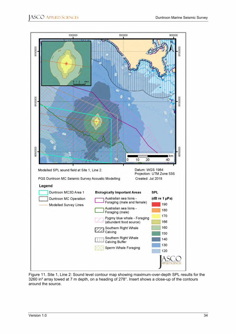
JASCO APPLIED SCIENCES Duntroon Marine Seismic Survey
Version 1.0 34
Figure 11. Site 1, Line 2: Sound level contour map showing maximum-over-depth SPL results for the 3260 in³ array towed at 7 m depth, on a heading of 278°. Insert shows a close-up of the contours around the source.

JASCO APPLIED SCIENCES Duntroon Marine Seismic Survey
Version 1.0 35
Figure 12. Site A: Sound level contour map showing unweighted maximum-over-depth per-pulse SEL results for the 3260 in³ array towed at 7 m depth, on a heading of 278°. Insert shows a close-up of the contours around the source.

JASCO APPLIED SCIENCES Duntroon Marine Seismic Survey
Version 1.0 36
Figure 13. Site A: Sound level contour map showing maximum-over-depth SPL results for the 3260 in³ array towed at 7 m depth, on a heading of 278°. Insert shows a close-up of the contours around the source.

JASCO APPLIED SCIENCES Duntroon Marine Seismic Survey
Version 1.0 37
Figure 14. Site B: Sound level contour map showing unweighted maximum-over-depth per-pulse SEL results for the 3260 in³ array towed at 7 m depth, on a heading of 278°. Insert shows a close-up of the contours around the source.
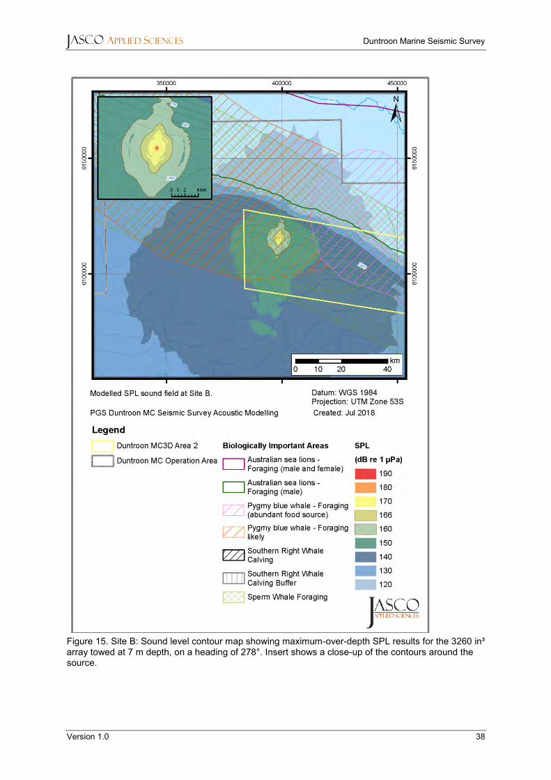
JASCO APPLIED SCIENCES Duntroon Marine Seismic Survey
Version 1.0 38
Figure 15. Site B: Sound level contour map showing maximum-over-depth SPL results for the 3260 in³ array towed at 7 m depth, on a heading of 278°. Insert shows a close-up of the contours around the source.

JASCO APPLIED SCIENCES Duntroon Marine Seismic Survey
Version 1.0 39
Figure 16. Line 2, Shot 5: Sound level contour map showing maximum-over-depth SPL results for the 3260 in³ array towed at 7 m depth, on a heading of 278° at the closest point to the SRW BIAs, receiver locations for sound levels at the boundaries are shown as circles. Insert shows a close-up of the contours around the source.

JASCO APPLIED SCIENCES Duntroon Marine Seismic Survey
Version 1.0 40
Figure 17. Line 2, Shot 5: Sound level contour map showing maximum-over-depth LF-weighted SPL results for the 3260 in³ array towed at 7 m depth, on a heading of 278° at the closest point to the SRW BIAs, receiver locations for sound levels at the boundaries are shown as circles. Insert shows a close-up of the contours around the source.

JASCO APPLIED SCIENCES Duntroon Marine Seismic Survey
Version 1.0 41
4.2.2.2. Entire water column: vertical slice
Figure 18. Site 1, Line 1: Predicted unweighted per-pulse SEL as vertical slices. Levels are shown in the broadside (top) and endfire directions (bottom). The source depth is 7 m and the tow direction is 098°.

JASCO APPLIED SCIENCES Duntroon Marine Seismic Survey
Version 1.0 42
Figure 19. Site 1, Line 1: Predicted unweighted SPL as vertical slices. Levels are shown in the broadside (top) and endfire directions (bottom). The source depth is 7 m and the tow direction is 098°.

JASCO APPLIED SCIENCES Duntroon Marine Seismic Survey
Version 1.0 43
Figure 20. Site 4, Line 1: Predicted unweighted per-pulse SEL as vertical slices. Levels are shown in the broadside (top) and endfire directions (bottom). The source depth is 7 m and the tow direction is 098°. White signifies below 120 dB.

JASCO APPLIED SCIENCES Duntroon Marine Seismic Survey
Version 1.0 44
Figure 21. Site 4, Line 1: Predicted unweighted SPL as vertical slices. Levels are shown in the broadside (top) and endfire directions (bottom). The source depth is 7 m and the tow direction is 098°.
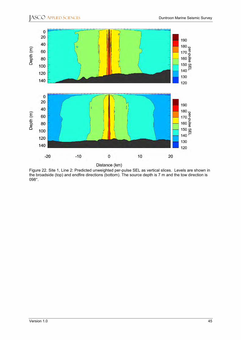
JASCO APPLIED SCIENCES Duntroon Marine Seismic Survey
Version 1.0 45
Figure 22. Site 1, Line 2: Predicted unweighted per-pulse SEL as vertical slices. Levels are shown in the broadside (top) and endfire directions (bottom). The source depth is 7 m and the tow direction is 098°.
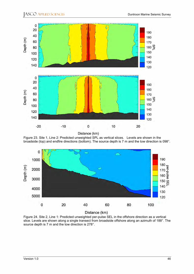
JASCO APPLIED SCIENCES Duntroon Marine Seismic Survey
Version 1.0 46
Figure 23. Site 1, Line 2: Predicted unweighted SPL as vertical slices. Levels are shown in the broadside (top) and endfire directions (bottom). The source depth is 7 m and the tow direction is 098°.
Figure 24. Site 2, Line 1: Predicted unweighted per-pulse SEL in the offshore direction as a vertical slice. Levels are shown along a single transect from broadside offshore along an azimuth of 188°. The source depth is 7 m and the tow direction is 278°.

JASCO APPLIED SCIENCES Duntroon Marine Seismic Survey
Version 1.0 47
Figure 25. Site 3, Line 2: Predicted unweighted SPL in the offshore direction as a vertical slice. Levels are shown along a single transect from broadside offshore along an azimuth of 188°. The source depth is 7 m and the tow direction is 278°.
Figure 26. Site A: Predicted unweighted per-pulse SEL as vertical slices. Levels are shown along a single transect from broadside towards shore (azimuth of 008°; top) and eastern endfire (azimuth of 098°; bottom). The source depth is 7 m and the tow direction is 278°.
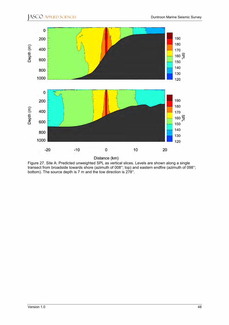
JASCO APPLIED SCIENCES Duntroon Marine Seismic Survey
Version 1.0 48
Figure 27. Site A: Predicted unweighted SPL as vertical slices. Levels are shown along a single transect from broadside towards shore (azimuth of 008°; top) and eastern endfire (azimuth of 098°; bottom). The source depth is 7 m and the tow direction is 278°.

JASCO APPLIED SCIENCES Duntroon Marine Seismic Survey
Version 1.0 49
Figure 28. Site B: Predicted unweighted per-pulse SEL as vertical slices. Levels are shown along a single transect from broadside towards shore (azimuth of 008°; top) and eastern endfire (azimuth of 098°; bottom). The source depth is 7 m and the tow direction is 278°.

JASCO APPLIED SCIENCES Duntroon Marine Seismic Survey
Version 1.0 50
Figure 29. Site B: Predicted unweighted SPL as vertical slices. Levels are shown along a single transect from broadside towards shore (azimuth of 008°; top) and eastern endfire (azimuth of 098°; bottom). The source depth is 7 m and the tow direction is 278°.
Figure 30. Site A: Predicted unweighted per-pulse SEL in the offshore direction as a vertical slice. Levels are shown along a single transect from broadside offshore along an azimuth of 188°. The source depth is 7 m and the tow direction is 278°.

JASCO APPLIED SCIENCES Duntroon Marine Seismic Survey
Version 1.0 51
Figure 31. Site A: Predicted SPL in the offshore direction as a vertical slice. Levels are shown along a single transect from broadside offshore along an azimuth of 188°. The source depth is 7 m and the tow direction is 278°. The purple line indicates water depth of 600 m.
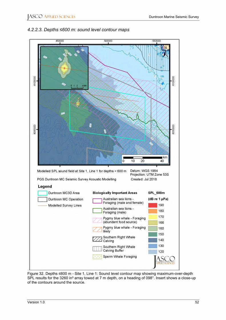
JASCO APPLIED SCIENCES Duntroon Marine Seismic Survey
Version 1.0 52
4.2.2.3. Depths ≤600 m: sound level contour maps
Figure 32. Depths ≤600 m - Site 1, Line 1: Sound level contour map showing maximum-over-depth SPL results for the 3260 in³ array towed at 7 m depth, on a heading of 098°. Insert shows a close-up of the contours around the source.

JASCO APPLIED SCIENCES Duntroon Marine Seismic Survey
Version 1.0 53
Figure 33. Depths ≤600 m - Site 4, Line 1: Sound level contour map showing maximum-over-depth SPL results for the 3260 in³ array towed at 7 m depth, on a heading of 098°. Insert shows a close-up of the contours around the source.

JASCO APPLIED SCIENCES Duntroon Marine Seismic Survey
Version 1.0 54
Figure 34. Depths ≤600 m - Site 1, Line 2: Sound level contour map showing maximum-over-depth SPL results for the 3260 in³ array towed at 7 m depth, on a heading of 278°. Insert shows a close-up of the contours around the source.

JASCO APPLIED SCIENCES Duntroon Marine Seismic Survey
Version 1.0 55
Figure 35. Depths ≤600 m - Site A: Sound level contour map showing maximum-over-depth SPL results for the 3260 in³ array towed at 7 m depth, on a heading of 278°. Insert shows a close-up of the contours around the source.

JASCO APPLIED SCIENCES Duntroon Marine Seismic Survey
Version 1.0 56
Figure 36. Depths ≤600 m - Site B: Sound level contour map showing maximum-over-depth SPL results for the 3260 in³ array towed at 7 m depth, on a heading of 278°. Insert shows a close-up of the contours around the source.

JASCO APPLIED SCIENCES Duntroon Marine Seismic Survey
Version 1.0 57
Figure 37. Site 1, Line 1: Sound level contour map comparing unweighted maximum-over-depth per-pulse SEL results for the entire water column and depths ≤600 m for the 3260 in³ array towed at 7 m depth, on a heading of 098°.

JASCO APPLIED SCIENCES Duntroon Marine Seismic Survey
Version 1.0 58
4.2.2.4. Seafloor levels
Figure 38. Predicted maximum PK along the seafloor at Sites C–F , depths at each site specified in the legend. Levels are the maximum of four transects, assessing both broadside and endfire directions. The source depth is 7 m.
Figure 39. Predicted maximum PK-PK along the seafloor at Sites C–F, depths at each site specified in the legend. Levels are the maximum of four transects, assessing both broadside and endfire directions. The source depth is 7 m.

JASCO APPLIED SCIENCES Duntroon Marine Seismic Survey
Version 1.0 59
4.3. Accumulated Sound Exposure Levels
The SEL24h results for acquisition within 3-D Survey Area 1 are presented in this section. Table 30 shows the estimated distances to the SEL-based injury and TTS criteria for marine mammals as per the NOAA Technical Guidance (NMFS 2018), along with the ensonified area. The results for the cumulative exposure criterion for potential TTS onset in fish in the water column and at the seafloor is shown in Table 31. Table 32 lists the estimated received level for each hearing group at the five sampling locations described in Table 5. The results for the SEL-based injury criteria (NMFS 2018) for low-frequency cetaceans considering only depths less than or equal to 600 m are shown in Table 33.
Maps displaying the corresponding sound fields and threshold contours for the entire water column are shown in Figures 40–44, while unweighted seafloor sound fields are shown in Figure 46. The sound levels associated with the accumulated SEL criteria for fish injury (Section 2.2) were not reached at the seafloor. Low-frequency cetacean weighted sound fields at depths less than or equal to 600 m and threshold contours are shown in Figure 45.
The modelled scenario assumes an impulse spacing of 16.67 m and that consecutive survey lines are 11.4 km apart. Higher received levels and longer distances to sound level thresholds could result if impulses or lines were closer together.
Tabulated Results
4.3.1.1. Entire water column
Table 30. Maximum-over-depth results for frequency-weighted SEL 24 h PTS thresholds based on the NOAA Technical Guidance (NMFS 2018) over the entire water column. A dash indicates that the threshold was not reached.
Hearing group
PTS TTS
Weighted SEL24h (LE,24h;
dB re 1 µPa²·s) Rmax (km) Area (km2)
Weighted SEL24h (LE,24h;
dB re 1 µPa²·s) Rmax (km) Area (km2)
Low-frequency cetaceans
183 0.76 160 168 88.1 6470
Mid-frequency cetaceans
185 – – 170 – –
High-frequency cetaceans
155 – – 140 0.14 38.5
Phocid pinnipeds in water
185 – – 170 0.27 54.9
Otariid pinnipeds in water
203 – – 188 – –
Table 31. Results for SEL24h fish TTS criteria (LE,24h; 186 dB re 1 µPa²·s), for the entire water column (maximum-over-depth) and seafloor receptors.
SEL24h isopleth (LE,24; dB re 1 µPa²·s)
Location Rmax (km) Area (km2)
186 Maximum-over-depth 4.97 823
Seafloor 4.92 780

JASCO APPLIED SCIENCES Duntroon Marine Seismic Survey
Version 1.0 60
Table 32. Received frequency-weighted SEL 24 h (LE,24h; dB re 1 µPa²·s) at five sampling locations. LF = Low-frequency cetaceans, MF = Mid-frequency cetaceans, HF = High-frequency cetaceans, PW = Phocid pinnipeds in water, OW = Otariid pinnipeds in water.
Location SEL
(LE,LF,24h)
SEL
(LE,MF,24h)
SEL
(LE,HF,24h)
SEL
(LE,PW,24h)
SEL
(LE,OW,24h)
1 Closest point between the array
and the sea lion BIAs 165.1 125.9 117.1 152.5 150.9
2 Closest point between the broadside of
the array and the sea lion BIAs 168.8 126.6 117.4 154.6 151.6
3 Closest point between the endfire of the
array and the sea lion BIAs 157.1 119.7 110.8 145.6 144.6
4 Closest point between the array
and the 100 m isobath 156.8 120.7 111.9 146.0 145.5
5 Closest point between the broadside of
the array and the 100 m isobath 160.3 120.7 111.8 147.2 145.5
4.3.1.2. Depths ≤600 m
Table 33. Depths ≤600 m: Maximum-over-depth results for frequency-weighted SEL 24 h (LE,24h; dB re 1 µPa²·s) thresholds based on the NOAA Technical Guidance (NMFS 2018) for water depths ≤600 m.
Hearing group Weighted SEL24h
(LE,24; dB re 1 µPa²·s)
PTS Weighted SEL24h (LE,24; dB re
1 µPa²·s)
TTS
Rmax (km) Area (km2) Rmax (km) Area (km2)
Low-frequency cetaceans
183 0.76 159 168 42.3 4,181

JASCO APPLIED SCIENCES Duntroon Marine Seismic Survey
Version 1.0 61
Sound Level Contour Maps
4.3.2.1. Entire water column
Figure 40. Low-frequency cetaceans (LF): Sound level contour map showing frequency-weighted maximum-over-depth SEL results accumulated over 24 h.

JASCO APPLIED SCIENCES Duntroon Marine Seismic Survey
Version 1.0 62
Figure 41. Mid-frequency cetaceans (MF): Sound level contour map showing frequency-weighted maximum-over-depth SEL results accumulated over 24 h.

JASCO APPLIED SCIENCES Duntroon Marine Seismic Survey
Version 1.0 63
Figure 42. High-frequency cetaceans (HF): Sound level contour map showing frequency-weighted maximum-over-depth SEL results accumulated over 24 h.
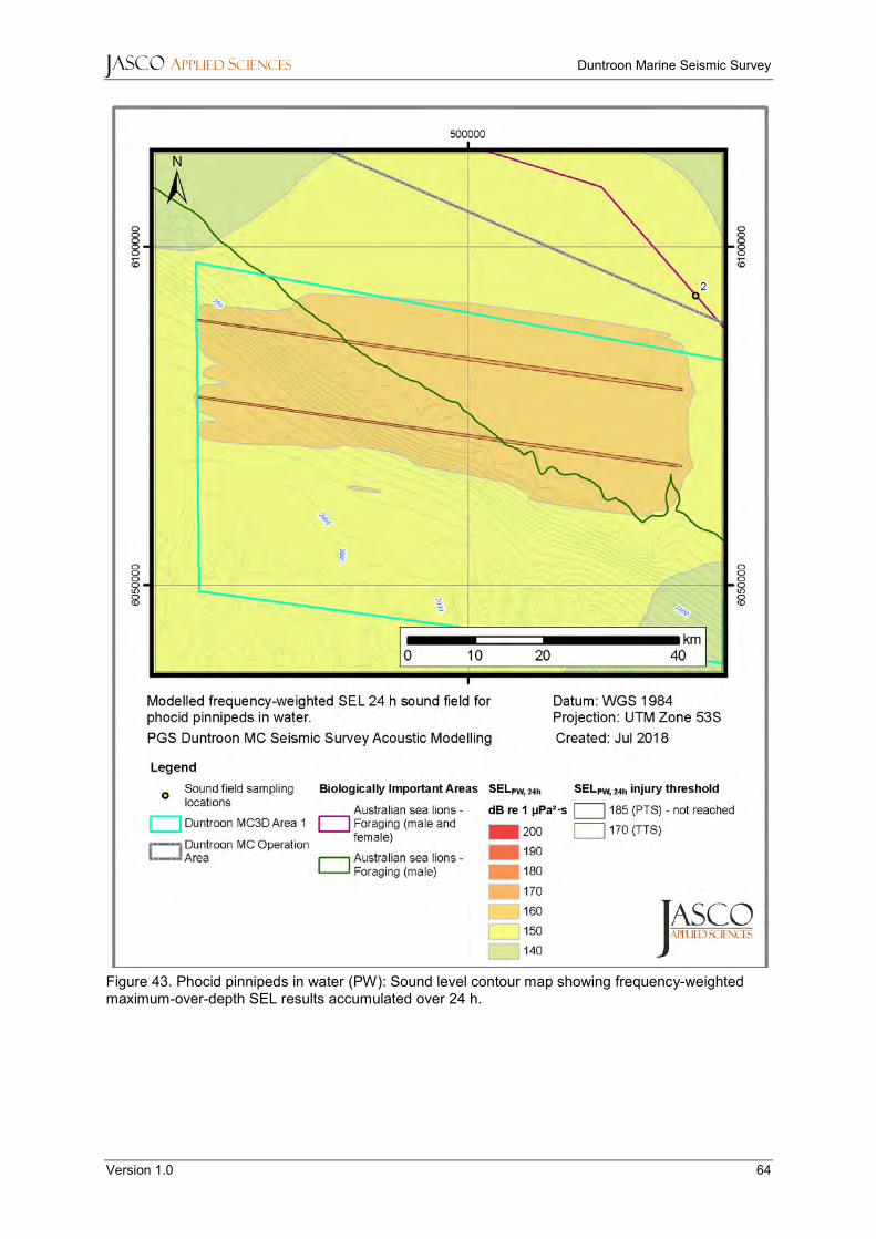
JASCO APPLIED SCIENCES Duntroon Marine Seismic Survey
Version 1.0 64
Figure 43. Phocid pinnipeds in water (PW): Sound level contour map showing frequency-weighted maximum-over-depth SEL results accumulated over 24 h.

JASCO APPLIED SCIENCES Duntroon Marine Seismic Survey
Version 1.0 65
Figure 44. Otariid pinnipeds in water (OW): Sound level contour map showing frequency-weighted maximum-over-depth SEL results accumulated over 24 h.

JASCO APPLIED SCIENCES Duntroon Marine Seismic Survey
Version 1.0 66
4.3.2.2. Depths ≤600 m
Figure 45. Depths ≤600 m: Low-frequency cetaceans (LF): Sound level contour map showing frequency-weighted maximum-over-depth SEL results accumulated over 24 h.

JASCO APPLIED SCIENCES Duntroon Marine Seismic Survey
Version 1.0 67
4.3.2.3. Seafloor
Figure 46. Sound level contour map showing unweighted seafloor SEL results accumulated over 24 h. The maximum distance to the seafloor 186 dB re 1 µPa²·s isopleth at the eastern boundary of the Southern Dogfish closure is 2.88 km.

JASCO APPLIED SCIENCES Duntroon Marine Seismic Survey
Version 1.0 68
5. Discussion and Conclusion
5.1. Overview
This modelling study predicted underwater sound levels associated with the 3-D component for PGS’s proposed Duntroon Marine Seismic Survey. The underwater sound field was modelled for a 3260 in3 airgun array (Appendix D.4) for water column sound speed profiles from May, the month with the highest noise transmission as determined from sound speed profiles (Appendix D.3.2). May was chosen to ensure precautionary estimates of distances to received sound level thresholds over the duration of the survey. The modelling also accounted for variations in site-specific bathymetry (Appendix D.3.1) and local geoacoustic properties (Appendix D.3.3).
The overall broadband (10–25000 Hz) unweighted per-pulse SEL source level of the 3260 in3 array was 224.9 dB re 1 µPa2·s in the broadside direction and 223.5 dB re 1 µPa2·s in the endfire direction. The peak pressure level in the same directions was 249.5 and 246.2 dB re 1 µPa respectively (Table 11); most of the acoustic energy is output at lower frequencies, in the tens to hundreds of hertz. Although there was little difference in the broadband source levels in the endfire and broadside directions, below a few hundred Hz some directivity caused slightly higher emissions in the broadside direction at those frequencies.
5.2. Single pulse sound fields
The modelling results for the Duntroon MSS reflect the nature of the bathymetry within the survey area, which encompasses the continental shelf, the shelf edge, and deep water within the GAB. The ranges to SEL isopleths associated with levels of 160 dB re 1 µPa2·s and higher typically decrease as the depth increases (Table 12).
The alignment of the acquisition lines with the continental shelf and the source directivity causes broadside lobes to propagate strongly in the offshore direction as depth increases. This is particularly noticeable in the SPL maps at Sites 1, 2, and 4, Line 1 (Figures 5, 7, and 9) and Site A (Figure 13). The modelled sites close to the shelf slope, which includes all Sites apart from Sites 1 and 5 on Line 1, and Sites 1 and 2 on Line 2, are all influenced by the presence of the slope. The presence of the slope supports long range propagation towards deeper water, which includes the western endfire and southern broadside directions. Site 3, Line 1, exhibits the strongest propagation in all offshore directions because depth increases with distance. While transmission loss is higher in the upslope direction, the strong directionality of the array typically results in distances to isopleths in the upslope direction still being greater than those in the endfire (along shelf break) direction. For the deepest site, Site 1, Line 1, the deep water reduces the reflection rate close to the source which limits the range to noise thresholds close to the source. At greater distances, however, the noise footprint is predominantly controlled by the bathymetry, with greater propagation towards deeper waters because less energy is lost to seabed interactions.
Prominent refractions and coherent focusing of sound in the southern broadside direction appear in the model results. These are illustrated in the examples at Site 2, Line 1 and Site A in the SPL maps (Figures 7 and 13), and the vertical slice plots which also include Site 3, Line 2 (Figures 24, 25, and 27). Sections of the footprint separated from the main coherent sound field can be described as ‘sound islands’. These are apparent in the aforementioned examples for isopleths of 160 dB re 1 µPa2·s and lower at long ranges are due to coherent focusing of sound in the homogeneous environment considered in the modelling. The environment is actually non-homogenous, with seafloor and sea surface roughness, along with localised variations in temperature and salinity. Therefore these ‘sound islands’, particularly the smaller ones, are not likely to exist, as the coherent focusing that creates them will be disrupted by scattering and refraction caused by roughness and inhomogeneities. To reduce the influence of the homogeneous modelling environment, range-dependent smoothing is applied according to the method of Harrison and Harrison (1995) to simulate the average transmission loss over the frequencies of each 1/3-octave-band (a Gaussian window with standard deviation of one quarter of the bandwidth was used). The outcome of the smoothing is likely a more realistic representation of what could be observed in a hon-homogeneous environment. The predicted per-pulse SEL and SPL Rmax radii in

JASCO APPLIED SCIENCES Duntroon Marine Seismic Survey
Version 1.0 69
Tables 12–17 for isopleths of 150 dB re 1 µPa2·s or 160 dB re 1 µPa and lower are not statistically representative of the sound field shape and extent, therefore the R95% distance is recommended for use in the impact assessment to represent distances to these isopleths.
As the water depth increases, the ensonified area at depths less than or equal to 600 m decreases (Table 26) due to the sound speed profile being downwards refracting from 50–1200 m, trapping more energy at lower depths. The corresponding Rmax distance is in some cases the same considering the entire water column or just depths ≤600 m, comparing Tables 12 and 21, this is because the bathymetry can influence the refraction of energy. For instance, if the modelling site is in close proximity to the slope, the influence of the slope causes upwards refraction in the upslope direction (Figure 18).
The closest modelled site to the Neptune Islands (Site 1, Line 2) results in a received level at a point midway between the islands, 76.6 km away, of 120 dB re 1 μPa (Table 18). The closest corner of point of the 3-D Survey Area 1 to this location is 61.7 km. The sound levels at the Neptune Islands if the array was to operate at the closest corner of point of 3-D Survey Area 1 are expected to be below 130 dB re 1 μPa (Figure 11). The closest modelled site to the SRW BIAs (Site 5, Line 2) results in received levels of 137 and 125 dB re 1 µPa at the boundaries of the calving buffer BIA and the calving BIA, respectively (Table 18). The LF-weighted SPL at the same locations is 4.2 and 3.2 dB lower than the unweighted equivalent, with the received levels being 132.8 and 121.8 dB re 1 µPa respectively (Table 19; Figure 17). Therefore the sound levels within the SRW BIAs are associated with a 10% probability of behavioural response according to the Wood et al. (2012) behavioural exposure criteria used in this analysis for calving and migrating SRW.
Considering the modelled sites in 3-D survey Area 1, The distance to the isopleth associated with the NMFS (2013) marine mammal behavioural response criterion of 160 dB re 1 µPa ranged from 6.08 to 9.78 km based on R95% distances, or 7.60 to 12.75 km based on Rmax distances (entire water column, Table 13), with the longest ranges occurred at the sites located around the shelf break. The minimum difference between the Rmax and R95% distances is 1.52 km (Site 1, Line 1), and the maximum is 6.5 km (Site 4, Line 2). However, as discussed previously, the R95% distances are recommended for this isopleth. The distances to the threshold for turtle behavioural response, 166 dB re 1 μPa (SPL) (NSF 2011), ranged from 2.82 to 4.32 km based on R95% distances, or 3.58 to 5.38 km based on Rmax distances (entire water column, Table 13). Considering only depths ≤600 m, the distances for turtle behavioural response ranged from 1.87 to 4.32 km based on R95% distances, or 2.25 to 5.38 km based on Rmax distances (depths ≤600 m, Table 22). Tables 25 and 27 present the total ensonified area for the entire water column and depths ≤600 m; the latter is more biologically relevant for determining the potential area of effect on mysticetes and turtles in terms of behavioural disturbance. This ensonified area is also more representative of the region of effect than the Rmax or R95% distances.
To place in context the modelled sites in 3-D Survey Area 2, A and B, with those at a similar depth in 3-D Survey Area 1, Line 1 Site 2 and Site 3, the resulting radii have been compared in Table 34. The radii for sound levels from 160 dB re 1 µPa²·s and higher are similar, with the greatest difference being 170 m. At lower sound levels and greater distances, the difference increases, which is due to the influence of the different bathymetry between the different locations. The bathymetry in 3-D Survey Area 2 has a more gradual slope when compared to that in 3-D Survey Area 1, where the slope is steeper.
The PK and PK-PK at the seafloor (Sections 4.2.1.3 and 4.2.2.4) were examined for comparison to criteria for fish (including sharks) (Section 2.2), and comparison the results in Payne et al. (2008), and Day et al. (2016a). As the sound levels associated with the accumulated SEL criteria for fish injury were not reached at the seafloor, the PK metric is the only relevant metric when considering the potential for injury. The PK metric associated with potential injury for fish without a swim bladder (applied to sharks in the absence of other information) was reached at the seafloor only at Site F (160 m deep), at a distance of 28 m from the centre of the array. At Site F, the distance for other categories of fish was 150 m. At Site C (200 m deep), only the criteria for fish with a swim bladder was reached, and the associated distance was 123 m (Table 28). The PK-PK metric from Payne et al. (2008), 202 dB re 1 µPa, was reached at all assessed sites (Table 29), with the maximum distance of 718 m occurring at Site C, due to the influence of the constructive critical angle bottom reflection (Figure 39).

JASCO APPLIED SCIENCES Duntroon Marine Seismic Survey
Version 1.0 70
Table 34. Comparison (distance) between maximum (Rmax) and 95% (R95%) horizontal distances (in m) from the 3260 in3 array to modelled maximum-over-depth per-pulse SEL isopleths between sites at similar depths in 3-D Survey Area 1 and 2 (Tables 12 and 14).
Per-pulse SEL (LE; dB re 1 µPa²·s)
Line 1, Site 3 compared to Site A (~500 m depth)
Line 1, Site 2 compared to Site B (~1000 m depth)
Rmax (m) R95% (m) Rmax (m) R95% (m)
190 0 0 0 0
180 0 0 0 0
170 −3 −1 1 0
160 10 6 170 0
5.3. Multiple pulse sound fields
This study also considered one scenario to assess the accumulated SEL of multiple airgun pulses over 24 hours of seismic operation, which was also based on the NMFS (2018) criteria. The model, which measured the cumulative effects of noise, considered the change in location and the azimuth of the source at each impulse point. The model predicts that unmitigated (no shut-downs) would result in effects criteria exceedance as follows:
• The PTS criteria were exceeded only for the low-frequency cetaceans, at a maximum horizontal distance of 760 m from each acquisition line (Table 30, Figure 40).
• TTS in pinnipeds was assessed to occur only in phocid pinnipeds, and at maximum horizontal distances of 270 m (Table 30, Figure 43). Therefore, TTS is not predicted to occur in otariid pinnipeds, a group that includes Australian sea lions (Figure 44).
Considering only depths ≤600 m (Table 33, Figure 45), the distance to the PTS criteria for low-frequency cetaceans remains the same. The Rmax for lower isopleths is also similar that for the entire water column and is determined by distances in the offshore direction. However, the total ensonified area at depths ≤600 m is significantly smaller for lower sound levels than it is for the entire water column, due to the downwards refracting sound speed profile. The Rmax is highly direction dependent and does not represent the ensonification distances along the slope nor on the continental shelf.
The 24-h SEL is a cumulative metric that reflects the dosimetric impact of noise levels within 24 hours based on the assumption that an animal is consistently exposed to such noise levels at a fixed position. The corresponding 24-h SEL radii for low-frequency cetaceans are larger than those for peak pressure criteria, but they represent an unlikely worst-case scenario. More realistically, marine mammals (or fish) would not stay in the same location or at the same range for 24 hours. Therefore, a reported radius for 24-h SEL criteria does not mean that marine fauna travelling within this radius of the source will be injured, but rather that an animal could be exposed to the sound level associated with injury (either PTS or TTS) if it remained in that range for 24 hours.
Location 2 (Table 32) had the highest received levels over 24 hours, this sound field sampling location was on the boundary of the male and female Australian sea lion BIA. This sampling location was exposed to the broadside aspect of the array while the seismic vessel was traversing both Lines 1 and 2, and therefore represents a worst case ensonification of the BIA. The SEL 24 h at this location for otariid pinnipeds was 151.6 dB re 1 µPa²·s. The received levels at both sampling locations on the 100 m isobath for otariid pinnipeds were identical (145.5 dB re 1 µPa²·s) and well below the TTS criterion. The maximum levels at the sampling location on the BIA boundary in the direction of Kangaroo Island (Location 3) was 144.6 dB re 1 µPa²·s for otariid pinnipeds and 157.1 dB re 1 µPa²·s for low-frequency cetaceans.

JASCO APPLIED SCIENCES Duntroon Marine Seismic Survey
Version 1.0 71
5.4. Summary
This section summarises the results in the context of the criteria and specific sound levels considered in the study (Section 2).
Marine Mammals
• NMFS (2018) marine mammal injury criteria: The results considered both metrics within the criteria for Permanent Threshold Shift (PTS) (PK and SEL24h). The furthest distance associated with either metric is required to be applied. The maximum distances along with the relevant metric and the location of the results are summarised in Table 35. Because the array is not a point source (8.8 × 16.8 m), the actual ranges from the edge of the airgun array are small for mid-frequency cetaceans, phocid and otariid pinnipeds.
• Based on the marine mammal injury criteria (NMFS 2018), temporary threshold shifts (non-injurious) in otariid pinnipeds such as the Australian sea lion are not predicted to occur at distances beyond the aperture of the array. However, TTS could occur in phocid pinnipeds at a maximum horizontal distance of 270 m from the 3260 in3 seismic airgun array, considering PK and SEL24h metrics (Tables 17 and Table 30).
• United States National Marine Fisheries Service (NMFS; 2013) acoustic threshold for behavioural effects in marine mammals: Airgun sounds exceeded the sound pressure level (SPL) threshold of 160 dB re 1 µPa for behavioural effects on marine mammals within 7.16 or 8.61 km of the 3260 in3 seismic airgun array (Tables 13 and 15, R95% distances) at the shallowest site (127 m, Site 1 Line 2) and Site A (496 m) respectively, considering the entire water column. The model represents best estimates of distances to the criteria, and although pockets of coherently-focussed sound do influence the Rmax results on a site dependent basis, the R95% distances are likely more representative of distances.
• Received sound levels at the boundary of the SRW calving and calving buffer BIAs were examined from the closest modelled site, and expressed in terms of unweighted and NMFS (2018) low-frequency (LF) weighted SPL. The LF weighted SPL is reported for comparison to the Wood et al. (2012) probabilistic disturbance threshold for migrating mysticetes, which have been demonstrated to respond to seismic airgun noise at lower received sound levels when compared to mysticetes in other behavioural states. The thresholds for migrating mysticetes are a 10% response likelihood at a weighted SPL of 120 dB re 1 µPa, 50% at a weighted SPL of 140 dB re 1 µPa, and a 90% response likelihood at a weighted SPL of 160 dB re 1 µPa.
o Unweighted sound levels at the boundaries of the calving buffer BIA and calving BIA are predicted to be 137 dB and 125 re 1 µPa (SPL), respectively (Figure 16; Table 18).
o LF-weighted sound levels at the boundaries of the calving buffer BIA and calving BIA are predicted to be 132.8 dB and 121.8 re 1 µPa (SPL), respectively (Figure 17; Table 19). This is associated with a 10% probability of behavioural response according to the Wood et al. (2012) behavioural exposure criteria used in this analysis for calving and migrating SRW.
Table 35. Summary of marine mammal PTS (injurious) onset distances. The per-pulse modelling resolution was 20 m.
Relevant hearing group Metric associated with PTS onset Distance Rmax (m) Result location
Low-frequency cetaceans†
SEL24h; LE,24h
760 Table 30
Low-frequency cetaceans in water depths ≤600m†
760 Table 30
Mid-frequency cetaceans
PK; Lpk
<20
Table 17 High-frequency cetaceans 450
Phocid pinnipeds in water 40
Otariid pinnipeds in water <20 † The model does not account for shutdowns.

JASCO APPLIED SCIENCES Duntroon Marine Seismic Survey
Version 1.0 72
Table 36. Summary of marine mammal TTS onset distances
Relevant hearing group Metric associated with
longest distance to TTS onset
Rmax (km) Result location
Low-frequency cetaceans†
SEL24h; LE,24h
88.1 Table 30
Low-frequency cetaceans in water depths ≤600m†
42.3 Table 30
Mid-frequency cetaceans
PK; Lpk
<0.02
Table 17 High-frequency cetaceans 0.98
Phocid pinnipeds in water 0.07
Otariid pinnipeds in water <0.02 † The model does not account for shutdowns.
Turtle Behaviour
• United States NMFS criterion for behavioural effects in turtles: Airgun sounds exceeded the 166 dB re 1 µPa SPL (Lp) threshold for behavioural effects within 1.87 to 4.32 km based on R95% distances, or 2.76 to 3.27 km based on Rmax distances at depths ≤600 m (Tables 22 and 24). Depths ≤600 m are likely more biologically relevant for turtles than those below 600 m.
Fish, Turtle Injury, Fish Eggs, and Fish Larvae
• Based on PK (Lpk) metrics, acoustic injury (including both lethal and recoverable injuries) could be sustained at the seafloor within a maximum horizontal distance of 28 m of the seismic array for fish without a swim bladder (Site F, 160 m deep) and within a maximum horizontal distance of 150 m for fish with a swim bladder, turtles, fish eggs, and fish larvae (160 m depth) (Table 28).
• The ranges associated with possible mortality, potential mortal injury, and recoverable injury to fish, turtles, fish eggs and larvae from Popper et al. (2014) using the SEL24h (LE,24) metric were not reached. As per the criteria, the PK metric should therefore be applied to assess these impacts to fish, turtles, fish eggs, and fish larvae.
• Considering the defined 24 hours of exposure, fish hearing could be temporarily impaired (TTS) within 4.92 km of the airgun array at the seafloor, and 4.97 km in the water column, based on the estimated horizontal Rmax radii (Table 31). The distances are determined from the shallower water sections of the lines, as in deeper water, the distance to criteria is shorter, being only 2.88 km at the eastern boundary of the Southern Gulper Shark closure area (Figure 46).
Crustaceans, Bivalves and Plankton
• To assist with the assessment of potential effects on crustaceans and bivalves, seafloor PK-PK was assessed at four locations, considering isopleths equivalent to those reported in Day et al. (2016a) along with the distance to a PK-PK of 202 dB re 1 µPa from Payne et al. (2007). The maximum distance to this sound level (202 dB re 1 µPa) is 718 m (Table 29).
• To assist with the assessment of potential effects on plankton, the distances to the sound level of 178 dB re 1 µPa PK-PK from McCauley et al. (2017) were estimated to range between 8 and 19.8 km at the five modelling sites based on Rmax distances and maximum-over-depth (Table 20).

JASCO APPLIED SCIENCES Duntroon Marine Seismic Survey
Version 1.0 73
Glossary
3-D
Three-dimensional
1/3-octave-band
Non-overlapping passbands that are one-third of an octave wide (where an octave is a doubling of frequency). Three adjacent 1/3-octave-bands comprise a one octave-band. One-third-octave-bands become wider with increasing frequency. Also see octave.
90% time window
The time interval over which the cumulative energy rises from 5% to 95% of the total pulse energy. This interval contains 90% of the total pulse energy. Symbol: T90.
90% sound pressure level (90% SPL)
The root-mean-square sound pressure levels calculated over the 90%-energy time window of a pulse. Used only for pulsed sounds.
attenuation
The gradual loss of acoustic energy from absorption and scattering as sound propagates through a medium.
audiogram
A graph of hearing threshold level (sound pressure levels) as a function of frequency, which describes the hearing sensitivity of an animal over its hearing range.
auditory weighting function (frequency-weighting function)
Auditory weighting functions account for marine mammal hearing sensitivity. They are applied to sound measurements to emphasise frequencies that an animal hears well and de-emphasise frequencies they hear less well or not at all (Southall et al. 2007, Finneran and Jenkins 2012, NOAA 2013).
azimuth
A horizontal angle relative to a reference direction, which is often magnetic north or the direction of travel. In navigation it is also called bearing.
bandwidth
The range of frequencies over which a sound occurs. Broadband refers to a source that produces sound over a broad range of frequencies (e.g., seismic airguns, vessels) whereas narrowband sources produce sounds over a narrow frequency range (e.g., sonar) (ANSI/ASA S1.13-2005 R2010).
bar
Unit of pressure equal to 100 kPa, which is approximately equal to the atmospheric pressure on Earth at sea level. 1 bar is equal to 106 Pa or 1011 µPa.
BIA
Biologically Important Area (http://www.environment.gov.au/marine/marine-species/bias)
broadside direction
Perpendicular to the travel direction of a source. Compare to endfire direction.
cetacean
Any animal in the order Cetacea. These are aquatic, mostly marine mammals and include whales, dolphins, and porpoises.
compressional wave
A mechanical vibration wave in which the direction of particle motion is parallel to the direction of propagation. Also called primary wave or P-wave.

JASCO APPLIED SCIENCES Duntroon Marine Seismic Survey
Version 1.0 74
decibel (dB)
One-tenth of a bel. Unit of level when the base of the logarithm is the tenth root of ten, and the quantities concerned are proportional to power (ANSI S1.1-1994 R2004).
endfire direction
Parallel to the travel direction of a source. Also see broadside direction.
ensonified area
The total area ensonified in conjunction with a specified isopleth.
frequency
The rate of oscillation of a periodic function measured in cycles-per-unit-time. The reciprocal of the period. Unit: hertz (Hz). Symbol: f. 1 Hz is equal to 1 cycle per second.
functional hearing group
Grouping of marine mammal species with similar estimated hearing ranges. Southall et al. (2007) proposed the following functional hearing groups: low-, mid-, and high-frequency cetaceans, pinnipeds in water, and pinnipeds in air.
geoacoustic
Relating to the acoustic properties of the seafloor.
GAB Great Australian Bight
hearing threshold
The sound pressure level that is barely audible for a given individual in the absence of significant background noise during a specific percentage of experimental trials.
hertz (Hz)
A unit of frequency defined as one cycle per second.
high-frequency cetacean
The functional hearing group that represents odontocetes specialised for using high frequencies.
impulsive sound
Sound that is typically brief and intermittent with rapid (within a few seconds) rise time and decay back to ambient levels (NOAA 2013, ANSI S12.7-1986 R2006). For example, seismic airguns and impact pile driving.
low-frequency cetacean
The functional hearing group that represents mysticetes (baleen whales).
maximum-over-depth (MOD)
The maximum value over all modelled depths above the sea floor.
mid-frequency cetacean
The functional hearing group that represents some odontocetes (dolphins, toothed whales, beaked whales, and bottlenose whales).
MC
Multi-Client
MSS
Marine Seismic Survey

JASCO APPLIED SCIENCES Duntroon Marine Seismic Survey
Version 1.0 75
mysticete
Mysticeti, a suborder of cetaceans, use their baleen plates, rather than teeth, to filter food from water. They are not known to echolocate but use sound for communication. Members of this group include rorquals (Balaenopteridae), right whales (Balaenidae), and the grey whale (Eschrichtius robustus).
non-impulsive sound
Sound that is broadband, narrowband or tonal, brief or prolonged, continuous or intermittent, and typically does not have a high peak pressure with rapid rise time (typically only small fluctuations in decibel level) that impulsive signals have (ANSI/ASA S3.20-1995 R2008). Marine vessels, aircraft, machinery, construction, and vibratory pile driving are examples.
octave
The interval between a sound and another sound with double or half the frequency. For example, one octave above 200 Hz is 400 Hz, and one octave below 200 Hz is 100 Hz.
odontocete
The presence of teeth, rather than baleen, characterises these whales. Members of the Odontoceti are a suborder of cetaceans, a group comprised of whales, dolphins, and porpoises. The toothed whales’ skulls are mostly asymmetric, an adaptation for their echolocation. This group includes sperm whales, killer whales, belugas, narwhals, dolphins, and porpoises.
parabolic equation method
A computationally-efficient solution to the acoustic wave equation that is used to model transmission loss. The parabolic equation approximation omits effects of back-scattered sound, simplifying the computation of transmission loss. The effect of back-scattered sound is negligible for most ocean-acoustic propagation problems.
peak pressure level (PK)
The maximum instantaneous sound pressure level, in a stated frequency band, within a stated period. Also called zero-to-peak pressure level. Unit: decibel (dB).
peak-to-peak pressure level (PK-PK)
The difference between the maximum and minimum instantaneous pressure levels. Unit: decibel (dB).
permanent threshold shift (PTS)
A permanent loss of hearing sensitivity caused by excessive noise exposure. PTS is considered auditory injury.
pinniped
A common term used to describe all three groups that form the superfamily Pinnipedia: phocids (true seals or earless seals), otariids (eared seals or fur seals and sea lions), and walrus.
point source
A source that radiates sound as if from a single point (ANSI S1.1-1994 R2004).
power spectrum density
The acoustic signal power per unit frequency as measured at a single frequency. Unit: µPa2/Hz, or µPa2·s.
power spectrum density level
The decibel level (10log10) of the power spectrum density, usually presented in 1 Hz bins. Unit: dB re 1 µPa2/Hz.
pressure, acoustic
The deviation from the ambient hydrostatic pressure caused by a sound wave. Also called overpressure. Unit: pascal (Pa). Symbol: p.

JASCO APPLIED SCIENCES Duntroon Marine Seismic Survey
Version 1.0 76
pulsed sound
Discrete sounds with durations less than a few seconds. Sounds with longer durations are called continuous sounds.
received level
The sound level measured at a receiver.
shear wave
A mechanical vibration wave in which the direction of particle motion is perpendicular to the direction of propagation. Also called secondary wave or S-wave. Shear waves propagate only in solid media, such as sediments or rock. Shear waves in the seafloor can be converted to compressional waves in water at the water-seafloor interface.
signature
Pressure signal generated by a source.
sound
A time-varying pressure disturbance generated by mechanical vibration waves travelling through a fluid medium such as air or water.
sound exposure
Time integral of squared, instantaneous frequency-weighted sound pressure over a stated time interval or event. Unit: pascal-squared second (Pa2·s) (ANSI S1.1-1994 R2004).
sound exposure level (SEL)
A cumulative measure related to the sound energy in one or more pulses. Unit: dB re 1 µPa2·s. SEL is expressed over the summation period (e.g., per-pulse SEL [for airguns], single-strike SEL [for pile drivers], 24-hour SEL).
sound field
Region containing sound waves (ANSI S1.1-1994 R2004).
sound pressure level (SPL)
The decibel ratio of the time-mean-square sound pressure, in a stated frequency band, to the square of the reference sound pressure (ANSI S1.1-1994 R2004).
For sound in water, the reference sound pressure is one micropascal (p0 = 1 µPa) and the unit for SPL is dB re 1 µPa:
( ) ( )010
2
0
2
10 /log20/log10SPL pppp ==
Unless otherwise stated, SPL refers to the root-mean-square sound pressure level. See also 90% sound pressure level and fast-average sound pressure level. Non-rectangular time window functions may be applied during calculation of the rms value, in which case the SPL unit should identify the window type.
sound speed profile
The speed of sound in the water column as a function of depth below the water surface.
source level (SL)
The sound pressure level or sound exposure level measured 1 metre from a theoretical point source that radiates the same total sound power as the actual source. Unit: dB re 1 μPa2m2 or dB 1 μPa2m2s.
spectrum
An acoustic signal represented in terms of its power (or energy) distribution versus frequency.
temporary threshold shift (TTS)
Temporary loss of hearing sensitivity caused by excessive noise exposure.

JASCO APPLIED SCIENCES Duntroon Marine Seismic Survey
Version 1.0 77
transmission loss (TL)
Also called propagation loss, this refers to the decibel reduction in sound level between two stated points that results from sound spreading away from an acoustic source subject to the influence of the surrounding environment.
wavelength
Distance over which a wave completes one oscillation cycle. Unit: meter (m). Symbol: λ.

JASCO APPLIED SCIENCES Duntroon Marine Seismic Survey
Version 1.0 78
Literature Cited
[DEWHA] Department of the Environment Water Heritage and the Arts. 2008. EPBC Act Policy Statement 2.1 - Interaction Between Offshore Seismic Exploration and Whales. In: Australian Government. Department of the Environment, W., Heritage and the Arts. 14 pp. http://www.environment.gov.au/resource/epbc-act-policy-statement-21-interaction-between-offshore-seismic-exploration-and-whales.
[HESS] High Energy Seismic Survey. 1999. High Energy Seismic Survey Review Process and Interim Operational Guidelines for Marine Surveys Offshore Southern California. Prepared for the California State Lands Commission and the United States Minerals Management Service Pacific Outer Continental Shelf Region by the High Energy Seismic Survey Team, Camarillo, California. 98 pp.
[ISO] International Organization for Standardization. 2016. ISO/DIS 18405.2:2017. Underwater acoustics—Terminology. Geneva. https://www.iso.org/standard/62406.html.
[NMFS] National Marine Fisheries Service. 1998. Acoustic Criteria Workshop. Dr. Roger Gentry and Dr. Jeanette Thomas Co-Chairs.
[NMFS] National Marine Fisheries Service. 2013. Marine Mammals: Interim Sound Threshold Guidance (webpage). National Marine Fisheries Service, National Oceanic and Atmospheric Administration, U.S. Department of Commerce. http://www.westcoast.fisheries.noaa.gov/protected_species/marine_mammals/threshold_guidance.html.
[NMFS] National Marine Fisheries Service. 2018. 2018 Revision to: Technical Guidance for Assessing the Effects of Anthropogenic Sound on Marine Mammal Hearing (Version 2.0): Underwater Thresholds for Onset of Permanent and Temporary Threshold Shifts. U.S. Department of Commerce, NOAA. NOAA Technical Memorandum NMFS-OPR-59, Silver Spring, MD. 167 pp. https://www.fisheries.noaa.gov/webdam/download/75962998.
[NOAA] National Oceanic and Atmospheric Administration. 2013. Draft guidance for assessing the effects of anthropogenic sound on marine mammals: Acoustic threshold levels for onset of permanent and temporary threshold shifts, December 2013, 76 pp. Silver Spring, Maryland: NMFS Office of Protected Resources. http://www.nmfs.noaa.gov/pr/acoustics/draft_acoustic_guidance_2013.pdf.
[NOAA] National Oceanic and Atmospheric Administration. 2015. Draft guidance for assessing the effects of anthropogenic sound on marine mammal hearing: Underwater acoustic threshold levels for onset of permanent and temporary threshold shifts, July 2015, 180 pp. Silver Spring, Maryland: NMFS Office of Protected Resources. http://www.nmfs.noaa.gov/pr/acoustics/draft%20acoustic%20guidance%20July%202015.pdf.
[NOAA] National Oceanic and Atmospheric Administration. 2016. Document Containing Proposed Changes to the NOAA Draft Guidance for Assessing the Effects of Anthropogenic Sound on Marine Mammal Hearing: Underwater Acoustic Threshold Levels for Onset of Permanent and Temporary Threshold Shifts, p. 24. http://www.nmfs.noaa.gov/pr/acoustics/draft_guidance_march_2016_.pdf.
[NSF] National Science Foundation (U.S.), U.S. Geological Survey, and [NOAA] National Oceanic and Atmospheric Administration (U.S.). 2011. Final Programmatic Environmental Impact Statement/Overseas. Environmental Impact Statement for Marine Seismic Research Funded by the National Science Foundation or Conducted by the U.S. Geological Survey. National Science Foundation, Arlington, VA.
[ONR] Office of Naval Research. 1998. ONR Workshop on the Effect of Anthropogenic Noise in the Marine Environment. Dr. R. Gisiner Chair.

JASCO APPLIED SCIENCES Duntroon Marine Seismic Survey
Version 1.0 79
Aerts, L., M. Blees, S. Blackwell, C. Greene, K. Kim, D. Hannay, and M. Austin. 2008. Marine mammal monitoring and mitigation during BP Liberty OBC seismic survey in Foggy Island Bay, Beaufort Sea, July-August 2008: 90-day report. Document Number LGL Report P1011-1. Report by LGL Alaska Research Associates Inc., LGL Ltd., Greeneridge Sciences Inc. and JASCO Applied Sciences for BP Exploration Alaska. 199 pp. http://www.nmfs.noaa.gov/pr/pdfs/permits/bp_liberty_monitoring.pdf.
ANSI S12.7-1986. R2006. American National Standard Methods for Measurements of Impulsive Noise. American National Standards Institute, New York.
ANSI S1.1-1994. R2004. American National Standard Acoustical Terminology. American National Standards Institute, New York.
ANSI S1.1-2013. R2013. American National Standard Acoustical Terminology. American National Standards Institute, New York.
ANSI/ASA S1.13-2005. R2010. American National Standard Measurement of Sound Pressure Levels in Air. American National Standards Institute and Acoustical Society of America, New York.
ANSI/ASA S3.20-1995. R2008. American National Standard Bioacoustical Terminology. American National Standards Institute and Acoustical Society of America, New York.
Bradshaw, B.E. 2002. Australian Geological Provinces: Duntroon Sub-basin (webpage). © Commonwealth of Australia (Geoscience Australia), Creative Commons Attribution 4.0 International Licence. http://www.ga.gov.au/provexplorer/provinceDetails.do?eno=27358.
Buckingham, M.J. 2005. Compressional and shear wave properties of marine sediments: Comparisons between theory and data. Journal of the Acoustical Society of America 117(1): 137-152. http://dx.doi.org/10.1121/1.1810231.
Carnes, M.R. 2009. Description and Evaluation of GDEM-V 3.0. Document Number NRL Memorandum Report 7330-09-9165. US Naval Research Laboratory, Stennis Space Center, MS. 21 pp.
Collins, M.D. 1993. A split-step Pade ́solution for the parabolic equation method. Journal of the Acoustical Society of America 93(4): 1736-1742.
Collins, M.D., R.J. Cederberg, D.B. King, and S. Chin-Bing. 1996. Comparison of algorithms for solving parabolic wave equations. Journal of the Acoustical Society of America 100(1): 178-182.
Coppens, A.B. 1981. Simple equations for the speed of sound in Neptunian waters. Journal of the Acoustical Society of America 69(3): 862-863. http://dx.doi.org/10.1121/1.385486.
Croll, D.A., A. Acevedo-Gutiérrez, B.R. Tershy, and J. Urbán-Ramı́rez. 2001. The diving behavior of blue and fin whales: is dive duration shorter than expected based on oxygen stores? Comparative Biochemistry and Physiology Part A: Molecular & Integrative Physiology 129(4): 797-809. http://www.sciencedirect.com/science/article/pii/S1095643301003488.
Day, R., D., R.D. McCauley, Q.P. Fitzgibbon, K. Hartmann, J.M. Semmens, and Institute for Marine and Antarctic Studies. 2016a. Assessing the Impact of Marine Seismic Surveys on Southeast Australian Scallop and Lobster Fisheries. FRDC Project No 2012/008. Impacts of Marine Seismic Surveys on Scallop and Lobster Fisheries. Fisheries Ressearch & Development Corporation, University of Tasmania, Hobart. 159 pp.
Day, R.D., R.D. McCauley, Q.P. Fitzgibbon, and J.M. Semmens. 2016b. Seismic air gun exposure during early-stage embryonic development does not negatively affect spiny lobster Jasus edwardsii larvae (Decapoda:Palinuridae). Scientific Reports 6: 1-9. http://dx.doi.org/10.1038/srep22723.

JASCO APPLIED SCIENCES Duntroon Marine Seismic Survey
Version 1.0 80
Dragoset, W.H. 1984. A comprehensive method for evaluating the design of airguns and airgun arrays. 16th Annual Proc. Offshore Tech. Conf. Volume 3. pp 75–84.
Duncan, A.J., A.N. Gavrilov, N. Alexander, R.D. McCauley, I.M. Parnum, and J.M. Collis. 2013. Characteristics of sound propagation in shallow water over an elastic seabed with a thin cap-rock layer. Journal of Acoustical Society of America 134(1): 207-215.
Ellison, W.T. and P.J. Stein. 1999. SURTASS LFA High Frequency Marine Mammal Monitoring (HF/M3) Sonar: Sustem Description and Test & Evaluation. Under U.S. Navy Contract N66604-98-D-5725.
Ellison, W.T. and A.S. Frankel. 2012. A common sense approach to source metrics. In Popper, A.N. and A. Hawkins (eds.). The Effects of Noise on Aquatic Life. Springer. pp 433-438.
Erbe, C., R. McCauley, and A. Gavrilov. 2016. Characterizing marine soundscapes. In Popper, N.A. and A. Hawkins (eds.). The Effects of Noise on Aquatic Life II. Springer New York, New York, NY. pp 265-271. http://dx.doi.org/10.1007/978-1-4939-2981-8_31.
Finneran, J.J. and C.E. Schlundt. 2010. Frequency-dependent and longitudinal changes in noise-induced hearing loss in a bottlenose dolphin (Tursiops truncatus). Journal of the Acoustical Society of America 128(2): 567-570.
Finneran, J.J. and A.K. Jenkins. 2012. Criteria and thresholds for U.S. Navy acoustic and explosive effects analysis. SPAWAR Systems Center Pacific, San Diego, California.
Finneran, J.J. 2015. Auditory weighting functions and TTS/PTS exposure functions for cetaceans and marine carnivores. San Diego: SSC Pacific.
Finneran, J.J. 2016. Auditory weighting functions and TTS/PTS exposure functions for marine mammals exposed to underwater noise. Technical Report. 49 pp.
Fisher, F.H. and V.P. Simmons. 1977. Sound absorption in sea water. Journal of the Acoustical Society of America 62(3): 558-564. http://link.aip.org/link/?JAS/62/558/1.
Funk, D., D. Hannay, D. Ireland, R. Rodrigues, and W. Koski (eds.). 2008. Marine mammal monitoring and mitigation during open water seismic exploration by Shell Offshore Inc. in the Chukchi and Beaufort Seas, July–November 2007: 90-day report. LGL Report P969-1. Prepared by LGL Alaska Research Associates Inc., LGL Ltd., and JASCO Research Ltd. for Shell Offshore Inc., National Marine Fisheries Service (US), and US Fish and Wildlife Service. 218 pp.
Gedamke, J., N. Gales, and S. Frydman. 2011. Assessing risk of baleen whale hearing loss from seismic surveys: The effect of uncertainty and individual variation. Journal of the Acoustical Society of America 129(1): 496-506. https://doi.org/10.1121/1.3493445.
Goldbogen, J.A., J. Calambokidis, E. Oleson, J. Potvin, N.D. Pyenson, G. Schorr, and R.E. Shadwick. 2011. Mechanics, hydrodynamics and energetics of blue whale lunge feeding: efficiency dependence on krill density. The Journal of Experimental Biology 214(4): 698-699. http://jeb.biologists.org/content/jexbio/214/4/698.full.pdf.
Hannay, D. and R. Racca. 2005. Acoustic Model Validation. Document Number 0000-S-90-04-T-7006-00-E, Revision 02. Technical report for Sakhalin Energy Investment Company Ltd. by JASCO Research Ltd. 34 pp.
Harrison, C.H. and J.A. Harrison. 1995. A simple relationship between frequency and range averages for broadband sonar. Journal of Acoustical Society of America 97(2): 1314-1317.
Heap, A.D. 2009. Marine Sediments (MARS) Database (webpage). Commonwealth of Australia (Geoscience Australia), Creative Commons Attribution 4.0 International Licence. http://www.ga.gov.au/metadata-gateway/metadata/record/gcat_69869.
JASCO APPLIED SCIENCES Duntroon Marine Seismic Survey
Version 1.0 81
Ireland, D.S., R. Rodrigues, D. Funk, W. Koski, and D. Hannay. 2009. Marine mammal monitoring and mitigation during open water seismic exploration by Shell Offshore Inc. in the Chukchi and Beaufort Seas, July–October 2008: 90-Day Report. Document Number LGL Report P1049-1. 277 pp.
Landro, M. 1992. Modeling of GI gun signatures. Geophysical Prospecting 40: 721–747.
Laws, R.M., L. Hatton, and M. Haartsen. 1990. Computer modeling of clustered airguns. First Break 8(9): 331–338.
Lucke, K., U. Siebert, P. Lepper, A., and M.-A. Blanchet. 2009. Temporary shift in masked hearing thresholds in a harbor porpoise (Phocoena phocoena) after exposure to seismic airgun stimuli. Journal of the Acoustical Society of America 125(6): 4060-4070.
Lurton, X. 2002. An Introduction to Underwater Acoustics: Principles and Applications. Springer, Chichester, U.K.
MacGillivray, A.O. and N.R. Chapman. 2012. Modeling underwater sound propagation from an airgun array using the parabolic equation method. Canadian Acoustics 40(1): 19-25. http://jcaa.caa-aca.ca/index.php/jcaa/article/view/2502.
Malme, C.I., P.R. Miles, C.W. Clark, P. Tyak, and J.E. Bird. 1983. Investigations of the Potential Effects of Underwater Noise from Petroleum Industry Activities on Migrating Gray Whale Behavior. Report Number 5366. http://www.boem.gov/BOEM-Newsroom/Library/Publications/1983/rpt5366.aspx.
Malme, C.I., P.R. Miles, C.W. Clark, P. Tyack, and J.E. Bird. 1984. Investigations of the Potential Effects of Underwater Noise from Petroleum Industry Activities on Migrating Gray Whale Behavior. Phase II: January 1984 migration. Report Number 5586. Bolt Beranek and Newman Inc. 357 pp.
Martin, B., K. Broker, M.-N.R. Matthews, J. MacDonnell, and L. Bailey. 2015. Comparison of measured and modeled air-gun array sound levels in Baffin Bay, West Greenland. OceanNoise 2015, 11-15 May, Barcelona, Spain.
Mattsson, A. and M. Jenkerson. 2008. Single Airgun and Cluster Measurement Project. Joint Industry Programme (JIP) on Exploration and Production Sound and Marine Life Proramme Review, October 28-30. International Association of Oil and Gas Producers, Houston, TX.
McCauley, R.D., J. Fewtrell, A.J. Duncan, C. Jenner, M.-N. Jenner, J.D. Penrose, R.I.T. Prince, A. Adihyta, J. Murdoch, et al. 2000. Marine seismic surveys: A study of environmental implications. Australian Petroleum Production Exploration Association (APPEA) Journal 40(1): 692-708. https://doi.org/10.1071/AJ99048.
McCauley, R.D., R.D. Day, K.M. Swadling, Q.P. Fitzgibbon, R.A. Watson, and J.M. Semmens. 2017. Widely used marine seismic survey air gun operations negatively impact zooplankton. 1: 0195. http://dx.doi.org/10.1038/s41559-017-0195.
McPherson, C.R., Z. Li, and M.-N.R. Matthews. 2017. Duntroon Marine Seismic Survey: Acoustic Modelling for Assessing Marine Fauna Sound Exposures. Document Number 01348. Version 2.0. Technical report by JASCO Applied Sciences for PGS Australia.
Moein, S.E., J.A. Musick, J.A. Keinath, D.E. Barnard, M.L. Lenhardt, and R. George. 1995. Evaluation of Seismic Sources for Repelling Sea Turtles from Hopper Dredges, in Sea Turtle Research Program: Summary Report. In: Hales, L.Z. (ed.). Report from U.S. Army Engineer Division, South Atlantic, Atlanta GA, and U.S. Naval Submarine Base, Kings Bay GA. Technical Report CERC-95. 90 pp.

JASCO APPLIED SCIENCES Duntroon Marine Seismic Survey
Version 1.0 82
Nedwell, J.R. and A.W. Turnpenny. 1998. The use of a generic frequency weighting scale in estimating environmental effect. Workshop on Seismics and Marine Mammals. 23–25th June 1998, London, U.K.
Nedwell, J.R., A.W.H. Turnpenny, J. Lovell, S.J. Parvin, R. Workman, and J.A.L. Spinks. 2007. A validation of the dBht as a measure of the behavioural and auditory effects of underwater noise. Report No. 534R1231 prepared by Subacoustech Ltd. for the UK Department of Business, Enterprise and Regulatory Reform under Project No. RDCZ/011/0004. www.subacoustech.com/information/downloads/reports/534R1231.pdf.
O'Neill, C., D. Leary, and A. McCrodan. 2010. Sound Source Verification. (Chapter 3) In Blees, M.K., K.G. Hartin, D.S. Ireland, and D. Hannay (eds.). Marine mammal monitoring and mitigation during open water seismic exploration by Statoil USA E&P Inc. in the Chukchi Sea, August-October 2010: 90-day report. LGL Report P1119. Prepared by LGL Alaska Research Associates Inc., LGL Ltd., and JASCO Applied Sciences Ltd. for Statoil USA E&P Inc., National Marine Fisheries Service (US), and US Fish and Wildlife Service. pp 1-34.
Owen, K., C.S. Jenner, M.-N.M. Jenner, and R.D. Andrews. 2016. A week in the life of a pygmy blue whale: migratory dive depth overlaps with large vessel drafts. Animal Biotelemetry 4(1): 17. https://doi.org/10.1186/s40317-016-0109-4
http://dx.doi.org/10.1186/s40317-016-0109-4.
Payne, J.F., C. Andrews, L. Fancey, A.L. Cook, and J.R. Christian. 2007. Pilot study on the effects of seismic air gun noise on lobster (Homarus americanus). Report Number 2712.
Payne, J.F., C. Andrews, L. Fancey, D. White, and J. Christian. 2008. Potential Effects of Seismic Energy on Fish and Shellfish: An Update since 2003. Report Number 2008/060. Canadian Science Advisory Secretariat. 22 pp.
Payne, R. and D. Webb. 1971. Orientation by means of long range acoustic signaling in baleen whales. Annals of the New York Academy of Sciences 188: 110-142. https://doi.org/10.1111/j.1749-6632.1971.tb13093.x.
Popper, A.N., A.D. Hawkins, R.R. Fay, D.A. Mann, S. Bartol, T.J. Carlson, S. Coombs, W.T. Ellison, R.L. Gentry, et al. 2014. Sound Exposure Guidelines for Fishes and Sea Turtles: A Technical Report prepared by ANSI-Accredited Standards Committee S3/SC1 and registered with ANSI. SpringerBriefs in Oceanography, Volume ASA S3/SC1.4 TR-2014. ASA Press.
Popper, A.N., T.J. Carlson, J.A. Gross, A.D. Hawkins, D. Zeddies, L. Powell, and J. Young. 2016. Effects of seismic air guns on pallid sturgeon and paddlefish. In Popper, A.N. and A. Hawkins (eds.). The Effects of Noise on Aquatic Life II. Volume 875. Springer, New York. pp 871-878. https://doi.org/10.1007/978-1-4939-2981-8_107.
Porter, M.B. and Y.-C. Liu. 1994. Finite-element ray tracing. In: Lee, D. and M.H. Schultz (eds.). Proceedings of the International Conference on Theoretical and Computational Acoustics. Volume 2. World Scientific Publishing Co. pp 947-956.
Racca, R., A. Rutenko, K. Bröker, and M. Austin. 2012a. A line in the water - design and enactment of a closed loop, model based sound level boundary estimation strategy for mitigation of behavioural impacts from a seismic survey. 11th European Conference on Underwater Acoustics 2012. Volume 34(3), Edinburgh, United Kingdom.
Racca, R., A. Rutenko, K. Bröker, and G. Gailey. 2012b. Model based sound level estimation and in-field adjustment for real-time mitigation of behavioural impacts from a seismic survey and post-event evaluation of sound exposure for individual whales. Acoustics 2012 Fremantle: Acoustics, Development and the Environment, Fremantle, Australia. http://www.acoustics.asn.au/conference_proceedings/AAS2012/papers/p92.pdf.

JASCO APPLIED SCIENCES Duntroon Marine Seismic Survey
Version 1.0 83
Southall, B.L., A.E. Bowles, W.T. Ellison, J.J. Finneran, R.L. Gentry, C.R. Greene, Jr., D. Kastak, D.R. Ketten, J.H. Miller, et al. 2007. Marine Mammal Noise Exposure Criteria: Initial Scientific Recommendations. Aquatic Mammals 33(4): 411-521.
Southall, B.L., D.P. Nowaceck, P.J.O. Miller, and P.L. Tyack. 2016. Experimental field studies to measure behavioral responses of cetaceans to sonar. Endangered Species Research 31: 293-315. https://doi.org/10.3354/esr00764.
Teague, W.J., M.J. Carron, and P.J. Hogan. 1990. A comparison between the Generalized Digital Environmental Model and Levitus climatologies. Journal of Geophysical Research 95(C5): 7167-7183.
Warner, G., C. Erbe, and D. Hannay. 2010. Underwater Sound Measurements. (Chapter 3) In Reiser, C.M., D.W. Funk, R. Rodrigues, and D. Hannay (eds.). Marine Mammal Monitoring and Mitigation during Open Water Shallow Hazards and Site Clearance Surveys by Shell Offshore Inc. in the Alaskan Chukchi Sea, July-October 2009: 90-Day Report. LGL Report P1112-1. Report by LGL Alaska Research Associates Inc. and JASCO Applied Sciences for Shell Offshore Inc., National Marine Fisheries Service (US), and US Fish and Wildlife Service. pp 1-54.
Whiteway, T. 2009. Australian Bathymetry and Topography Grid, June 2009. GeoScience Australia, Canberra. http://www.ga.gov.au/metadata-gateway/metadata/record/gcat_67703.
Wood, J., B.L. Southall, and D.J. Tollit. 2012. PG&E offshore 3 D Seismic Survey Project EIR-Marine Mammal Technical Draft Report. SMRU Ltd.
Zhang, Y. and C. Tindle. 1995. Improved equivalent fluid approximations for a low shear speed ocean bottom. Journal of the Acoustical Society of America 98(6): 3391-3396. https://doi.org/10.1121/1.413789.
Ziolkowski, A. 1970. A method for calculating the output pressure waveform from an air gun. Geophysical Journal of the Royal Astronomical Society 21(2): 137-161.

JASCO APPLIED SCIENCES Duntroon Marine Seismic Survey
Version 1.0 A-1
Appendix A. Acoustic Metrics
Underwater sound pressure amplitude is measured in decibels (dB) relative to a fixed reference pressure of p0 = 1 μPa. Because the perceived loudness of sound, especially impulsive noise such as from seismic airguns, pile driving, and sonar, is not generally proportional to the instantaneous acoustic pressure, several sound level metrics are commonly used to evaluate noise and its effects on marine life. We provide specific definitions of relevant metrics used in the accompanying report. Where possible we follow the ANSI and ISO standard definitions and symbols for sound metrics, but these standards are not always consistent.
The zero-to-peak sound pressure level (PK; Lpk; Lp,pk; dB re 1 µPa), is the maximum instantaneous sound pressure level in a stated frequency band attained by an acoustic pressure signal, p(t):
(A-1)
PK is often included as a criterion for assessing whether a sound is potentially injurious; however, because it does not account for the duration of a noise event, it is generally a poor indicator of perceived loudness.
The peak-to-peak sound pressure level (PK-PK; Lpk-pk; Lp,pk-pk; dB re 1 µPa) is the difference between the maximum and minimum instantaneous sound pressure levels in a stated frequency band attained by an impulsive sound, p(t):
(A-2)
The sound pressure level (SPL; Lp; dB re 1 µPa) is the rms pressure level in a stated frequency band over a specified time window (T, s) containing the acoustic event of interest. It is important to note that SPL always refers to an rms pressure level and therefore not instantaneous pressure:
(A-3)
where g(t) is an optional time weighting function. The SPL represents a nominal effective continuous sound over the duration of an acoustic event, such as the emission of one acoustic pulse, a marine mammal vocalisation, the passage of a vessel, or over a fixed duration. Because the window length, T, is the divisor, events with similar sound exposure level (SEL) but more spread out in time have a lower SPL.
In studies of impulsive noise, the time window function g(t) is often a decaying exponential that emphasizes more recent pressure signals to mimic the leaky integration of the mammalian hearing system. For example, human-based fast time weighting applies an exponential function with time constant 125 ms. Another approach for evaluating Lp of impulsive signals is to set T to the “90% time window” (T90): the period over which cumulative square pressure function passes between 5% and 95% of its full per-pulse value. The SPL computed over this T90 interval is commonly called the 90% SPL (SPL(T90); Lp90; dB re 1 µPa):
(A-4)
( )( )
=
0
10,
maxlog20
p
tpL pkp
( ) ( )
−
=− 2
0
2
10,
)(min)(maxlog10
p
tptpL pkpkp
=
2
0
2
10 )(1
log10 pdttpT
LT
p
=
2
0
2
90
1090
90
)(1
log10 pdttpT
LT
p

JASCO APPLIED SCIENCES Duntroon Marine Seismic Survey
Version 1.0 A-2
The sound exposure level (SEL; LE; LE,p; dB re 1 µPa2·s) is a measure related to the acoustic energy contained in one or more acoustic events (N). The SEL for a single event is computed from the time-integral of the squared pressure over the full event duration (T):
(A-5)
where T0 is a reference time interval of 1 s. The SEL continues to increase with time when non-zero pressure signals are present. It therefore can be construed as a dose-type measurement, so the integration time used must be carefully considered in terms of relevance for impact to the exposed recipients.
SEL can be calculated over periods with multiple acoustic events or over a fixed duration. For a fixed duration, the square pressure is integrated over the duration of interest. For multiple events, the SEL can be computed by summing (in linear units) the SEL of the N individual events:
. (A-6)
To compute the SPL(T90) and SEL of acoustic events in the presence of high levels of background noise, equations A-4 and A-5 are modified to subtract the background noise contribution:
(A-7)
(A-8)
where is the mean square pressure of the background noise, generally computed by averaging the squared pressure of a temporally-proximal segment of the acoustic recording during which acoustic events are absent (e.g., between pulses).
Because the SPL(T90) and SEL are both computed from the integral of square pressure, these metrics are related by the following expression, which depends only on the duration of the time window T:
(A-9)
(A-10)
where the 0.458 dB factor accounts for the 10% of SEL missing from the SPL(T90) integration time window.
If applied, the frequency weighting of an acoustic event should be specified, as in the case of LF-weighted SEL (e.g., LE,LF,24h; Appendix A.2). The use of fast, slow, or impulse exponential-time-averaging or other time-related characteristics should else be specified.
A.1. Marine Mammal Impact Criteria
Marine mammals can be adversely affected by underwater anthropogenic noise. Payne and Webb (1971) suggested that communication distances of fin whales are reduced by shipping sounds. Subsequently, similar concerns arose regarding effects of other underwater noise sources and the possibility that impulsive sources—primarily airguns used in seismic surveys—could cause auditory injury. This led to a series of workshops held in the late 1990s, conducted to address acoustic mitigation requirements for seismic surveys and other underwater noise sources (NMFS 1998, ONR
=
2
00
2
10 )(log10 pTdttpLT
E
=
=
N
i
NE
iE
L1
10
L
10,
,
10log10
−=
2
0
22
90
1090
90
))((1
log10 pdtntpT
LT
p
−=
2
00
22
10 ))((log10 pTdtntpLT
E
2n
( )TLL Ep 10log10−=
( ) 458.0log10 901090 −−= TLL Ep

JASCO APPLIED SCIENCES Duntroon Marine Seismic Survey
Version 1.0 A-3
1998, Nedwell and Turnpenny 1998, HESS 1999, Ellison and Stein 1999). In the years since these early workshops, a variety of thresholds have been proposed for both injury) and disturbance (Section 2.1.2). The following sections summarise the recent development of thresholds; however, this field remains an active research topic.
A.1.1. Injury In recognition of shortcomings of the SPL-only based injury criteria, in 2005 NMFS sponsored the Noise Criteria Group to review literature on marine mammal hearing to propose new noise exposure criteria. Some members of this expert group published a landmark paper (Southall et al. 2007) that suggested assessment methods similar to those applied for humans. The resulting recommendations introduced dual acoustic injury criteria for impulsive sounds that included peak pressure level thresholds and SEL24h thresholds, where the subscripted 24h refers to the accumulation period for calculating SEL. The peak pressure level criterion is not frequency weighted whereas the SEL24h is frequency weighted according to one of four marine mammal species hearing groups: Low-, Mid- and High-Frequency cetaceans (LF, MF, and HF respectively) and Pinnipeds in Water (PINN). These weighting functions are referred to as M-weighting filters (analogous to the A-weighting filter for human; Appendix A.2). The SEL24h thresholds were obtained by extrapolating measurements of onset levels of Temporary Threshold Shift (TTS) in belugas by the amount of TTS required to produce Permanent Threshold Shift (PTS) in chinchillas. The Southall et al. (2007) recommendations do not specify an exchange rate, which suggests that the thresholds are the same regardless of the duration of exposure (i.e., it implies a 3 dB exchange rate).
Wood et al. (2012) refined Southall et al.’s (2007) thresholds, suggesting lower injury values for LF and HF cetaceans while retaining the filter shapes. Their revised thresholds were based on TTS-onset levels in harbour porpoises from Lucke et al. (2009), which led to a revised impulsive sound PTS threshold for HF cetaceans of 179 dB re 1 µPa2·s. Because there were no data available for baleen whales, Wood et al. (2012) based their recommendations for LF on results obtained from MF studies. In particular they referenced Finneran and Schlundt (2010) research, which found mid-frequency cetaceans are more sensitive to non-impulsive sound exposure than Southall et al. (2007) assumed. Wood et al. (2012) thus recommended a more conservative TTS-onset level for LF cetaceans of 192 dB re 1 µPa2·s.
As of 2017, an optimal approach is not apparent. There is consensus in the research community that an SEL-based method is preferable either separately or in addition to an SPL-based approach to assess the potential for injuries. In August 2016, after substantial public and expert input into three draft versions and based largely on the above-mentioned literature (NOAA 2013, 2015, 2016), NMFS finalised technical guidance for assessing the effect of anthropogenic sound on marine mammal hearing (NMFS 2018). The guidance describes injury criteria with new thresholds and frequency weighting functions for the five hearing groups described by Finneran and Jenkins (2012). Table A-1 lists the recommended thresholds. The criteria defined in NMFS (2018) are applied in this report.
Table A-1. Marine mammal injury (PTS onset) thresholds based on NMFS (2018).
Hearing group Impulsive source Non-impulsive source
PK Weighted SEL (24 h) Weighted SEL (24 h)
Low-frequency cetaceans 219 183 199
Mid-frequency cetaceans 230 185 198
High-frequency cetaceans 202 155 173
Phocid pinnipeds in water 218 185 201
Otariid pinnipeds in water 232 203 219

JASCO APPLIED SCIENCES Duntroon Marine Seismic Survey
Version 1.0 A-4
A.2. Marine Mammal Frequency Weighting
The potential for noise to affect animals depends on how well the animals can hear it. Noises are less likely to disturb or injure an animal if they are at frequencies that the animal cannot hear well. An exception occurs when the sound pressure is so high that it can physically injure an animal by non-auditory means (i.e., barotrauma). For sound levels below such extremes, the importance of sound components at particular frequencies can be scaled by frequency weighting relevant to an animal’s sensitivity to those frequencies (Nedwell and Turnpenny 1998, Nedwell et al. 2007).
A.2.1. Marine Mammal Frequency Weighting Functions
In 2015, a U.S. Navy technical report by Finneran (2015) recommended new auditory weighting functions. The overall shape of the auditory weighting functions is similar to human A-weighting functions, which follows the sensitivity of the human ear at low sound levels. The new frequency-weighting function is expressed as:
( ) ( )
+++=
b
hi
a
lo
a
lo
ffff
ffKfG
22
2
10
11
)(log10)( (A-11)
Finneran (2015) proposed five functional hearing groups for marine mammals in water: low-, mid-, and high-frequency cetaceans, phocid pinnipeds, and otariid pinnipeds. The parameters for these frequency-weighting functions were further modified the following year (Finneran 2016) and were adopted in NOAA’s technical guidance that assesses noise impacts on marine mammals (NMFS 2018). Table A-2 lists the frequency-weighting parameters for each hearing group; Figure A-1 shows the resulting frequency-weighting curves.
Table A-2. Parameters for the auditory weighting functions recommended by NMFS (2018).
Hearing group a b flo (Hz) fhi (kHz) K (dB)
Low-frequency cetaceans
1.0 2 200 19,000 0.13
Mid-frequency cetaceans
1.6 2 8,800 110,000 1.20
High-frequency cetaceans
1.8 2 12,000 140,000 1.36
Phocid pinnipeds in water
1.0 2 1,900 30,000 0.75
Otariid pinnipeds in water
2.0 2 940 25,000 0.64

JASCO APPLIED SCIENCES Duntroon Marine Seismic Survey
Version 1.0 A-5
Figure A-1. Auditory weighting functions for functional marine mammal hearing groups as recommended by NMFS (2018).

JASCO APPLIED SCIENCES Duntroon Marine Seismic Survey
Version 1.0 B-1
Appendix B. Acoustic Source Model
B.1. Methods
The source levels and directivity of the airgun array were predicted with JASCO’s Airgun Array Source Model (AASM). AASM includes low- and high-frequency modules for predicting different components of the airgun array spectrum. The low-frequency module is based on the physics of oscillation and radiation of airgun bubbles, as originally described by Ziolkowski (1970), that solves the set of parallel differential equations that govern bubble oscillations. Physical effects accounted for in the simulation include pressure interactions between airguns, port throttling, bubble damping, and generator-injector (GI) gun behaviour discussed by Dragoset (1984), Laws et al. (1990), and Landro (1992). A global optimisation algorithm tunes free parameters in the model to a large library of airgun source signatures.
Whilst airgun signatures are highly repeatable at the low frequencies, which are used for seismic imaging, their sound emissions have a large random component at higher frequencies that cannot be predicted deterministically. Therefore, the high-frequency module of AASM uses a stochastic simulation to predict the sound emissions of individual airguns above 800 Hz, using a multivariate statistical model. The current version of AASM has been tuned to fit a large library of high quality seismic source signature data obtained from the Joint Industry Program (JIP) on Sound and Marine Life (Mattsson and Jenkerson 2008). The stochastic model uses a Monte-Carlo simulation of the random component of the high-frequency spectrum of each airgun in an array. The mean high-frequency spectra from the stochastic model augment the low-frequency signatures from the physical model, allowing AASM to predict airgun source levels at frequencies up to 25,000 Hz.
AASM produces a set of “notional” signatures for each array element based on:
• Array layout
• Volume, tow depth, and firing pressure of each airgun
• Interactions between different airguns in the array
These notional signatures are the pressure waveforms of the individual airguns at a standard reference distance of 1 m; they account for the interactions with the other airguns in the array. The signatures are summed with the appropriate phase delays to obtain the far-field source signature of the entire array in all directions. This far-field array signature is filtered into 1/3-octave-bands to compute the source levels of the array as a function of frequency band and azimuthal angle in the horizontal plane (at the source depth), after which it is considered to be a directional point source in the far field.
A seismic array consists of many sources and the point-source assumption is invalid in the near field where the array elements add incoherently. The maximum extent of the near field of an array (Rnf) is:
4
2
nf
lR
(B-1)
where λ is the sound wavelength and l is the longest dimension of the array (Lurton 2002, §5.2.4). For example, an airgun array length of l = 21 m yields a near-field range of 147 m at 2 kHz and 7 m at 100 Hz. Beyond this Rnf range, the array is assumed to radiate like a directional point source and is treated as such for propagation modelling.
The interactions between individual elements of the array create directionality in the overall acoustic emission. Generally, this directionality is prominent mainly at frequencies in the mid-range between tens of hertz to several hundred hertz. At lower frequencies, with acoustic wavelengths much larger than the inter-airgun separation distances, the directionality is small. At higher frequencies, the pattern of lobes is too finely spaced to be resolved and the effective directivity is less.

JASCO APPLIED SCIENCES Duntroon Marine Seismic Survey
Version 1.0 B-2
B.2. Acoustic Source Levels and Directivity Results
Figure B-1 shows the broadside (perpendicular to the tow direction), endfire (parallel to the tow direction), and vertical overpressure signatures and corresponding power spectrum levels for the 3260 in3 array. The signatures consist of a strong primary peak, related to the initial release of high-pressure air, followed by a series of pulses associated with bubble oscillations. Most energy is produced at frequencies below 600 Hz. Frequency-dependent peaks and nulls in the spectrum result from interference among airguns in the array and correspond with the volumes and relative locations of the airguns to each other.
Horizontal 1/3-octave-band source levels are shown as a function of band centre frequency and azimuth (Figure B-2); directivity in the sound field is most noticeable at mid-frequencies as described in the model detail in Appendix B.1.
Figure B-1. Predicted source level details for the 3260 in3 array towed at a depth of 7 m. (Left) the overpressure signature and (right) the power spectrum for broadside (perpendicular to tow direction) and endfire (directly aft of the array) directions, and for vertically down.

JASCO APPLIED SCIENCES Duntroon Marine Seismic Survey
Version 1.0 B-3
Figure B-2. Directionality of the predicted horizontal source levels for the 3260 in3 array, 5–2000 Hz. Source levels (in dB re 1 µPa2·s) are shown as a function of azimuth for the centre frequencies of the 1/3-octave-bands modelled; frequencies are shown above the plots. Tow direction is to the right. Tow depth is 7 m (see Table D-2)

JASCO APPLIED SCIENCES Duntroon Marine Seismic Survey
Version 1.0 C-1
Appendix C. Sound Propagation Models
C.1. MONM-BELLHOP
Underwater sound propagation (i.e., transmission loss) was predicted with JASCO’s Marine Operations Noise Model (MONM). This model computes sound propagation at frequencies of 5 Hz to 1.25 kHz via a wide-angle parabolic equation solution to the acoustic wave equation (Collins 1993) based on a version of the U.S. Naval Research Laboratory’s Range-dependent Acoustic Model (RAM), which has been modified to account for a solid seabed (Zhang and Tindle 1995). MONM computes sound propagation at frequencies > 1.25 kHz via the BELLHOP Gaussian beam acoustic ray-trace model (Porter and Liu 1994).
The parabolic equation method has been extensively benchmarked and is widely employed in the underwater acoustics community (Collins et al. 1996). MONM accounts for the additional reflection loss at the seabed, which results from partial conversion of incident compressional waves to shear waves at the seabed and sub-bottom interfaces, and it includes wave attenuations in all layers. MONM incorporates the following site-specific environmental properties: a bathymetric grid of the modelled area, underwater sound speed as a function of depth, and a geoacoustic profile based on the overall stratified composition of the seafloor.
This version of MONM accounts for sound attenuation due to energy absorption through ion relaxation and viscosity of water in addition to acoustic attenuation due to reflection at the medium boundaries and internal layers (Fisher and Simmons 1977). The former type of sound attenuation is significant for frequencies higher than 5 kHz and cannot be neglected without noticeably affecting the model results.
MONM computes acoustic fields in three dimensions by modelling transmission loss within two-dimensional (2-D) vertical planes aligned along radials covering a 360° swath from the source, an approach commonly referred to as N×2-D. These vertical radial planes are separated by an angular step size of , yielding N = 360°/ number of planes (Figure C-1).
Figure C-1. The N×2-D and maximum-over-depth modelling approach used by MONM.
MONM treats frequency dependence by computing acoustic transmission loss at the centre frequencies of 1/3-octave-bands. Range-dependent smoothing is applied according to the method of Harrison and Harrison (1995) to simulate the average transmission loss over the frequencies of each 1/3-octave-band (a Gaussian window with standard deviation of one quarter of the bandwidth was

JASCO APPLIED SCIENCES Duntroon Marine Seismic Survey
Version 1.0 C-2
used). Sufficiently many 1/3-octave-bands, starting at 10 Hz, are modelled to include most acoustic energy emitted by the source. At each centre frequency, the transmission loss is modelled within each of the N vertical planes as a function of depth and range from the source. The 1/3-octave-band received per-pulse SELs are computed by subtracting the band transmission loss values from the directional source level in that frequency band. Composite broadband received SELs are then computed by summing the received 1/3-octave-band levels.
The received per-pulse SEL sound field within each vertical radial plane is sampled at various ranges from the source, generally with a fixed radial step size. At each sampling range along the surface, the sound field is sampled at various depths, with the step size between samples increasing with depth below the surface. The step sizes are chosen to provide increased coverage near the depth of the source and at depths of interest in terms of the sound speed profile. For areas with deep water, sampling is not performed at depths beyond those reachable by marine mammals. The received per-pulse SEL at a surface sampling receiver location is taken as the maximum value that occurs over all samples within the water column, i.e., the maximum-over-depth received per-pulse SEL. These maximum-over-depth per-pulse SELs are presented as colour contours around the source.
MONM’s predictions have been validated against experimental data from several underwater acoustic measurement programs conducted by JASCO (Hannay and Racca 2005, Aerts et al. 2008, Funk et al. 2008, Ireland et al. 2009, O'Neill et al. 2010, Warner et al. 2010, Racca et al. 2012a, Racca et al. 2012b, Martin et al. 2015).
C.2. FWRAM
For impulsive sounds from the seismic array, time-domain representations of the pressure waves generated in the water are required to calculate SPL and peak pressure level. Furthermore, the airgun array must be represented as a distributed source to accurately characterise vertical directivity effects in the near-field zone. For this study, synthetic pressure waveforms were computed using FWRAM, which is a time-domain acoustic model based on the same wide-angle parabolic equation (PE) algorithm as MONM. FWRAM computes synthetic pressure waveforms versus range and depth for range-varying marine acoustic environments, and it takes the same environmental inputs as MONM (bathymetry, water sound speed profile, and seafloor geoacoustic profile). Unlike MONM, FWRAM computes pressure waveforms via Fourier synthesis of the modelled acoustic transfer function in closely spaced frequency bands. FWRAM employs the array starter method to accurately model sound propagation from a spatially distributed source (MacGillivray and Chapman 2012).
Besides providing direct calculations of the peak pressure level and SPL, the synthetic waveforms from FWRAM can also be used to convert the SEL values from MONM to SPL.
C.3. Wavenumber Integration Model
Sound pressure levels near the airgun array were modelled using JASCO’s VSTACK wavenumber integration model. VSTACK computes synthetic pressure waveforms versus depth and range for arbitrarily layered, range-independent acoustic environments using the wavenumber integration approach to solving the exact (range-independent) acoustic wave equation. This model is valid over the full angular range of the wave equation and can fully account for the elasto-acoustic properties of the sub-bottom. Wavenumber integration methods are extensively used in the field of underwater acoustics and seismology where they are often referred to as reflectivity methods or discrete wavenumber methods. VSTACK computes sound propagation in arbitrarily stratified water and seabed layers by decomposing the outgoing field into a continuum of outward-propagating plane cylindrical waves. Seabed reflectivity in the model is dependent on the seabed layer properties: compressional and shear wave speeds, attenuation coefficients, and layer densities. The output of the model can be post-processed to yield estimates of the SEL, SPL, and PK.
VSTACK accurately predicts steep-angle propagation in the proximity of the source but is computationally slow at predicting sound pressures at large distances due to the need for smaller wavenumber steps with increasing distance. Additionally, VSTACK assumes range-invariant bathymetry with a horizontally stratified medium (i.e., a range-independent environment), which is azimuthally symmetric about the source. VSTACK is thus best suited to modelling the sound field near the source.

JASCO APPLIED SCIENCES Duntroon Marine Seismic Survey
Version 1.0 D-1
Appendix D. Methods and Parameters
This section describes the specifications of the airgun array source that was used at all sites and the environmental parameters used in the propagation models.
D.1. Estimating Range to Thresholds Levels
Sound level contours were calculated based on the underwater sound fields predicted by the propagation models, sampled by taking the maximum value over all modelled depths above the sea floor for each location in the modelled region. The predicted distances to specific levels were computed from these contours. Two distances relative to the source are reported for each sound level: 1) Rmax, the maximum range to the given sound level over all azimuths, and 2) R95%, the range to the given sound level after the 5% farthest points were excluded (see examples in Figure D-1).
The R95% is used because sound field footprints are often irregular in shape. In some cases, a sound level contour might have small protrusions or anomalous isolated fringes. This is demonstrated in the image in Figure D-1(a). In cases such as this, where relatively few points are excluded in any given direction, Rmax can misrepresent the area of the region exposed to such effects, and R95% is considered more representative. In strongly asymmetric cases such as shown in Figure D-1(b), on the other hand, R95% neglects to account for significant protrusions in the footprint. In such cases Rmax might better represent the region of effect in specific directions. Cases such as this are usually associated with bathymetric features affecting propagation. The difference between Rmax and R95% depends on the source directivity and the non-uniformity of the acoustic environment.
(a) (b) Figure D-1. Sample areas ensonified to an arbitrary sound level with Rmax and R95% ranges shown for two different scenarios. (a) Largely symmetric sound level contour with small protrusions. (b) Strongly asymmetric sound level contour with long protrusions. Light blue indicates the ensonified areas bounded by R95%; darker blue indicates the areas outside this boundary which determine Rmax.
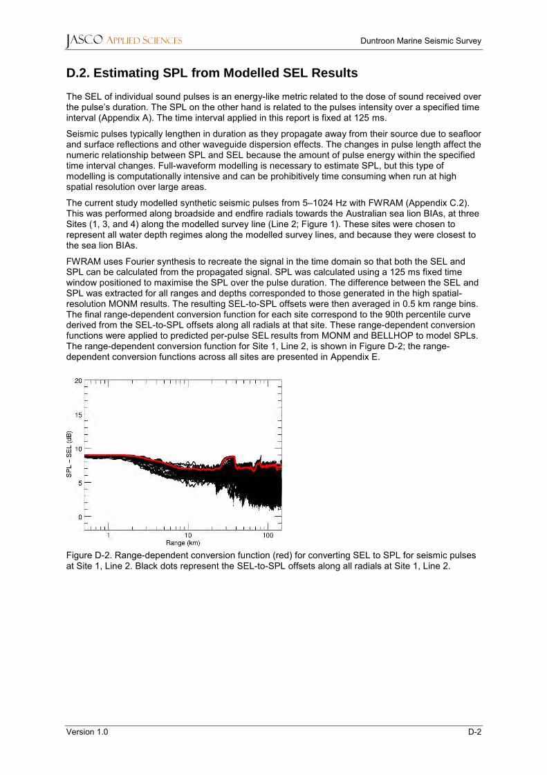
JASCO APPLIED SCIENCES Duntroon Marine Seismic Survey
Version 1.0 D-2
D.2. Estimating SPL from Modelled SEL Results
The SEL of individual sound pulses is an energy-like metric related to the dose of sound received over the pulse’s duration. The SPL on the other hand is related to the pulses intensity over a specified time interval (Appendix A). The time interval applied in this report is fixed at 125 ms.
Seismic pulses typically lengthen in duration as they propagate away from their source due to seafloor and surface reflections and other waveguide dispersion effects. The changes in pulse length affect the numeric relationship between SPL and SEL because the amount of pulse energy within the specified time interval changes. Full-waveform modelling is necessary to estimate SPL, but this type of modelling is computationally intensive and can be prohibitively time consuming when run at high spatial resolution over large areas.
The current study modelled synthetic seismic pulses from 5–1024 Hz with FWRAM (Appendix C.2). This was performed along broadside and endfire radials towards the Australian sea lion BIAs, at three Sites (1, 3, and 4) along the modelled survey line (Line 2; Figure 1). These sites were chosen to represent all water depth regimes along the modelled survey lines, and because they were closest to the sea lion BIAs.
FWRAM uses Fourier synthesis to recreate the signal in the time domain so that both the SEL and SPL can be calculated from the propagated signal. SPL was calculated using a 125 ms fixed time window positioned to maximise the SPL over the pulse duration. The difference between the SEL and SPL was extracted for all ranges and depths corresponded to those generated in the high spatial-resolution MONM results. The resulting SEL-to-SPL offsets were then averaged in 0.5 km range bins. The final range-dependent conversion function for each site correspond to the 90th percentile curve derived from the SEL-to-SPL offsets along all radials at that site. These range-dependent conversion functions were applied to predicted per-pulse SEL results from MONM and BELLHOP to model SPLs. The range-dependent conversion function for Site 1, Line 2, is shown in Figure D-2; the range-dependent conversion functions across all sites are presented in Appendix E.
Figure D-2. Range-dependent conversion function (red) for converting SEL to SPL for seismic pulses at Site 1, Line 2. Black dots represent the SEL-to-SPL offsets along all radials at Site 1, Line 2.

JASCO APPLIED SCIENCES Duntroon Marine Seismic Survey
Version 1.0 D-3
D.3. Environmental Parameters
D.3.1. Bathymetry Water depths throughout the modelled area were extracted from the Australian Bathymetry and Topography Grid, a 9 arc-second grid (approximately 250 × 280 m to 270 × 280 m at the studied latitudes) rendered for Australian waters (Whiteway 2009) (Figure 1). Bathymetry data were extracted and re-gridded onto a Universal Transverse Mercator (UTM) coordinate projections appropriate for all sites with a regular grid spacing of 100 × 100 m, which describes all sites in this study.
D.3.2. Sound speed profile The sound speed profiles for the modelled sites were derived from temperature and salinity profiles from the U.S. Naval Oceanographic Office’s Generalized Digital Environmental Model V 3.0 (GDEM; Teague et al. 1990, Carnes 2009). GDEM provides an ocean climatology of temperature and salinity for the world’s oceans on a latitude-longitude grid with 0.25° resolution, with a temporal resolution of one month, based on global historical observations from the U.S. Navy’s Master Oceanographic Observational Data Set (MOODS). The temperature and salinity profiles were converted to sound speed profiles according to the equations of Coppens (1981).
The sound speed profiles for March, April, May, September, October, and November were calculated at five locations within the operation area and at one location farther offshore to examine the most conservative profile during the possible survey time period. The mean profiles of the five locations for each month were compared to determine which produced the most conservative scenario (Figure D-3). Since the profiles did not extend to the maximum water depth in the modelling area, they were supplemented with a deeper nearby offshore profile.
The sound speed profile for May provided the greatest propagation; the profile typically features a well-mixed layer with a slight upward-refracting gradient at 0-40 m. The sound speed profile between 50 and ~1200 m depth is downward refracting, but upward refracting at greater depths. The resulting profile was input to the sound propagation modelling (Figure D-3).

JASCO APPLIED SCIENCES Duntroon Marine Seismic Survey
Version 1.0 D-4
Figure D-3. The mean sound speed profiles for May, September, October, and November: full water depth (left), <500 m (right) at all sites. The profiles were calculated from temperature and salinity profiles from GDEM V 3.0 (GDEM; Teague et al. 1990, Carnes 2009).

JASCO APPLIED SCIENCES Duntroon Marine Seismic Survey
Version 1.0 D-5
D.3.3. Geoacoustics Geoacoustic parameters used in acoustic transmission loss modelling were derived from sedimentary grain size measurements from the Australian Government’s Marine Sediments (MARS) database (Heap 2009). Most of these samples were taken on or near the seafloor, although some are from sediment at greater depths. On average, the surficial grain size indicates silty sand is present throughout the modelled area. Geotechnical data along the southern Australian shelf typically show sand overlaying calcarenite layers (Bradshaw 2002, Duncan et al. 2013). Representative grain sizes and porosity were used in the grain-shearing model proposed by Buckingham (2005) to estimate the geoacoustic parameters required by the sound propagation models. Table D-1 lists the geoacoustic parameters used for numeric modelling.
Table D-1. Geoacoustic profile used as the input to the models at all sites.
Depth below seafloor (m)
Material Density (g/cm3)
P-wave speed (m/s)
P-wave attenuation (dB/λ)
S-wave speed (m/s)
S-wave attenuation (dB/λ)
0–10
Silty sand to semi-cemented limestone
1.88 1605–1700 0.35–0.70
255 3.65
10–20 1.88–1.89 1700–1755 0.70–0.85
20–50 1.89–1.90 1755–1850 0.85–1.15
50–100 1.90–1.92 1850–1950 1.15–1.35
100–200 1.92–1.96 1950–2100 1.35–1.60
200–500 1.96–2.05 2100–2355 1.60–1.95
>500 2.05 2355 1.95
D.4. Acoustic Source
The model considered the following specifications:
• A 3260 in³ firing volume seismic airgun array.
• Bolt 1900 LLXT airguns operated at a firing pressure of 2000 psi.
• An 8.8 × 16.8 m array layout consisting of three strings towed at a 7.0 m depth (Figure D-4, Table D-2).
Figure D-4. Layout of the modelled 3260 in3 airgun array. Tow depth is 7 m. The labels indicate the firing volume (in cubic inches) for each airgun. The convention is that the array is towed in the positive x direction. Also see Table D-2.

JASCO APPLIED SCIENCES Duntroon Marine Seismic Survey
Version 1.0 D-6
Table D-2. Layout of the modelled 3260 in3 airgun array. Tow depth is 7 m. Firing pressure for all guns is 2000 psi. The tow direction is assumed to be in the positive x direction. Also see Figure D-4.
Gun x (m) y (m) Volume (in3) Gun x (m) y (m) Volume (in3)
1 7 −4.4 90 13 7 3.6 150
2 7 −3.6 90 14 7 4.4 150
3 4 −4.4 150 15 4 4 100
4 4 −3.6 150 (spare) 16 2 4 40
5 2 −4.4 250 17 0 3.6 250
6 2 −3.6 250 18 0 4.4 250
7 0 −4.4 150 19 −2 3.6 60
8 0 −3.6 150 20 −2 4.4 60
9 −2 −4 250 21 −4 3.6 250
10 −4 −4 70 22 −4 4.4 250 (spare)
11 −7 −4.4 150 23 −7 3.6 100
12 −7 −3.6 150 24 −7 4.4 100

JASCO APPLIED SCIENCES Duntroon Marine Seismic Survey
Version 1.0 E-1
Appendix E. FWRAM Results
To generate SEL to SPL conversion factors and model distances to PK thresholds, FWRAM was run along three transects: endfire and the two broadside transects. FWRAM computes synthetic pressure waveforms versus range and depth using the PE approach. It computes pressure waveforms via Fourier synthesis of the modelled acoustic transfer function in closely spaced frequency bands. Because of the intensity of the computation, this model was run up to a frequency of 1024 Hz, and at three sites along survey line 2, closest to the Australian sea lion Biological Important Areas (BIAs). The conversion factors were applied at the nine modelled sites based on similarity in water depth.
The conversion factors were the same values calculated in the previous modelling (McPherson et al. 2017) since the array sizes are similar and the locations are the same. Each conversion factor was calculated from the generated SEL and SPL values for the 3090 in3 array along three transects. The conversion factors as a function of range are shown in Figures D-1 to D-3. The black dots indicate the spread of the difference between the two metrics. The red lines represent the 90th percentile of the range-dependent difference that was used in the modelling results presented.
Modelling results for the synthetic pressure waveforms can be viewed as time domain traces, in which multipath arrivals for each impulse can be seen. Figures E-6 to E-8 show example traces for Site 3, Line 2. The 125 ms fixed time window is positioned to maximise the SPL over the pulse duration. If the actual environment is less homogenous than that used as the modelling input, the multipath arrivals could be more distributed in time, thus reducing the SPL within the fixed time window.
Figure E-1. Conversion Factor 1, applied to sites with water depths of 127–250 m: Range-dependent conversion function for converting single-pulse SEL to SPL for the 3090 in3 airgun array.
Figure E-2. Conversion Factor 2, applied to sites with water depths of 250–550 m: Range-dependent conversion function for converting single-pulse SEL to SPL for the 3090 in3 airgun array.
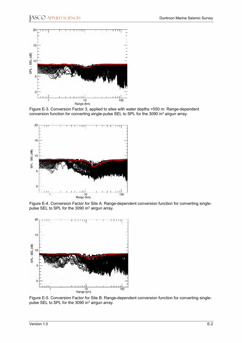
JASCO APPLIED SCIENCES Duntroon Marine Seismic Survey
Version 1.0 E-2
Figure E-3. Conversion Factor 3, applied to sites with water depths >550 m: Range-dependent conversion function for converting single-pulse SEL to SPL for the 3090 in3 airgun array.
Figure E-4. Conversion Factor for Site A: Range-dependent conversion function for converting single-pulse SEL to SPL for the 3090 in3 airgun array.
Figure E-5. Conversion Factor for Site B: Range-dependent conversion function for converting single-pulse SEL to SPL for the 3090 in3 airgun array.

JASCO APPLIED SCIENCES Duntroon Marine Seismic Survey
Version 1.0 E-3
Figure E-6. FWRAM modelled pressure traces in the northern broadside direction for Site 3, Line 2. Results are for the 3260 in3 airgun array, 0 s time represents the time of airgun array firing. The grey shading highlights the location of the 125 ms fixed time window.
Figure E-7. FWRAM modelled pressure traces in the southern broadside direction for Site 3, Line 2. Results are for the 3260 in3 airgun array, 0 s time represents the time of airgun array firing. The grey shading highlights the location of the 125 ms fixed time window.

JASCO APPLIED SCIENCES Duntroon Marine Seismic Survey
Version 1.0 E-4
Figure E-8. FWRAM modelled pressure traces in the eastern endfire direction for Site 3, Line 2. Results are for the 3260 in3 airgun array, 0 s time represents the time of airgun array firing. The grey shading highlights the location of the 125 ms fixed time window.

Version 1.0 DRAFT i
Duntroon Marine Seismic Survey
Animal Movement Modelling for Assessing Marine Fauna Sound Exposures for a 3260 in³ array
Submitted to: Alyse Blake PGS Australia
Authors: Klaus Lucke Sam Denes Craig McPherson Jennifer Wladichuk
20 September 2018
P001361-002 Document 01657 Version 1.0 DRAFT
JASCO Applied Sciences (Australia) Pty Ltd Unit 1, 14 Hook Street
Capalaba, Queensland, 4157 Tel: +61 7 3823 2620
Mob: +61 4 3812 8179 www.jasco.com
Version 1.0 DRAFT i
Document Version Control
Version Date Name Change
1.0 20 Sept 2018 C. McPherson Draft submitted to client
Suggested citation:
Lucke, K., S. Denes, C. McPherson and J. Wladichuk, J. 2018. Duntroon Marine Seismic Survey: Animal Movement Modelling for Assessing Marine Fauna Sound Exposures for a 3260 in³ array. Document 01657, Version 1.0 DRAFT. Technical report by JASCO Applied Sciences for PGS Australia.
Disclaimer:
The results presented herein are relevant within the specific context described in this report. They could be misinterpreted if not considered in the light of all the information contained in this report. Accordingly, if information from this report is used in documents released to the public or to regulatory bodies, such documents must clearly cite the original report, which shall be made readily available to the recipients in integral and unedited form.
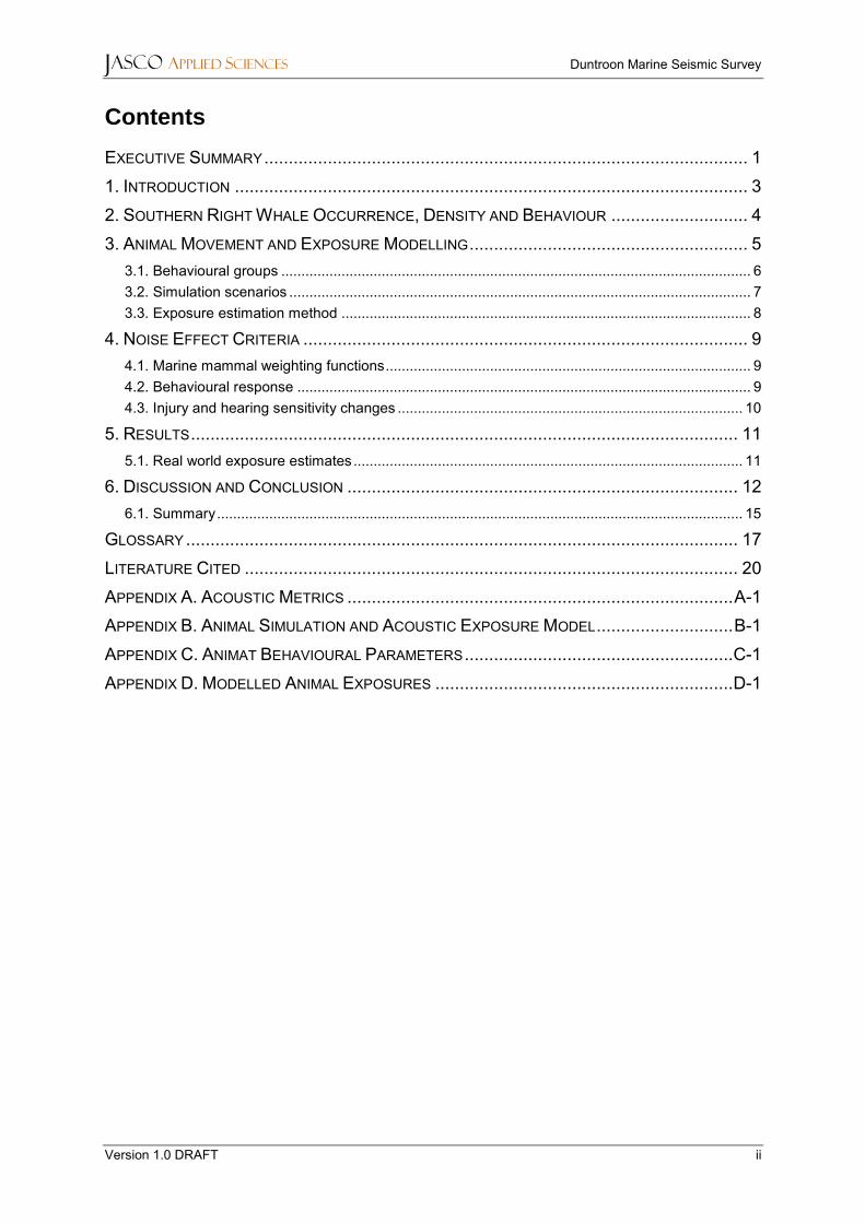
JASCO APPLIED SCIENCES Duntroon Marine Seismic Survey
Version 1.0 DRAFT ii
Contents
EXECUTIVE SUMMARY ................................................................................................... 1
1. INTRODUCTION ......................................................................................................... 3
2. SOUTHERN RIGHT WHALE OCCURRENCE, DENSITY AND BEHAVIOUR ............................ 4
3. ANIMAL MOVEMENT AND EXPOSURE MODELLING ......................................................... 5 3.1. Behavioural groups ..................................................................................................................... 6 3.2. Simulation scenarios ................................................................................................................... 7 3.3. Exposure estimation method ...................................................................................................... 8
4. NOISE EFFECT CRITERIA ........................................................................................... 9 4.1. Marine mammal weighting functions ........................................................................................... 9 4.2. Behavioural response ................................................................................................................. 9 4.3. Injury and hearing sensitivity changes ...................................................................................... 10
5. RESULTS ................................................................................................................ 11 5.1. Real world exposure estimates ................................................................................................. 11
6. DISCUSSION AND CONCLUSION ................................................................................ 12 6.1. Summary ................................................................................................................................... 15
GLOSSARY ................................................................................................................. 17
LITERATURE CITED ..................................................................................................... 20
APPENDIX A. ACOUSTIC METRICS ............................................................................... A-1
APPENDIX B. ANIMAL SIMULATION AND ACOUSTIC EXPOSURE MODEL ............................ B-1
APPENDIX C. ANIMAT BEHAVIOURAL PARAMETERS ....................................................... C-1
APPENDIX D. MODELLED ANIMAL EXPOSURES ............................................................. D-1

JASCO APPLIED SCIENCES Duntroon Marine Seismic Survey
Version 1.0 DRAFT iii
Figures
Figure 1. Site locations and relevant features for the Duntroon MSS 3-D Survey Area 1 (Figure 1; Wladichuk et al. 2018). ...................................................................................................................... 3
Figure 2. Cartoon of animats in a moving sound field. ........................................................................... 6 Figure 3. Map showing the operations area and the animat seeding boundaries. Nearshore SRW
animats were seeded between the 20m contour and the coast. Offshore SRW were seeded between the 5000 m contour and the 20 m contour. ......................................................................... 7
Figure 4. Sound level contour map showing maximum-over-depth LF-weighted SPL results for the 3260 in³ array towed at 7 m depth, operating at Line 2, Shot 5, on a heading of 278° at the closest point to the SRW BIAs ......................................................................................................... 14
Figure 5. Sound level contour map focused on the footprint closer to the coast, showing maximum-over-depth LF-weighted SPL results for the 3260 in³ array towed at 7 m depth, operating at Line 2, Shot 5, on a heading of 278° at the closest point to the SRW BIAs ................ 15
Tables
Table 1. Behavioural exposure criteria used in this analysis for calving and migrating southern right whales ...................................................................................................................................... 10
Table 2. The SEL24h (LE,24h) and PK (Lpk) thresholds for acoustic effects on southern right whales. ... 10 Table 3. Spatial scaling of animat modelling results for entire SRW population. ................................. 11 Table 4. Spatial scaling of animat modelling results for eastern SRW population. .............................. 11 Table 5. Predicted, scaled number of animat exposed to sound pressure levels exceeding
behavioural disturbance criteria for eastern and entire SRW (sub-)population during the 24 h simulation. ........................................................................................................................................ 16
Table 6. Predicted, scaled number of animat exposed to sound exposure levels exceeding the TTS and PTS criteria from NMFS (2018) for entire and eastern SRW (sub-)population during the 24 h simulation. .......................................................................................................................... 16
Table 7. Population-scaling of animat modelling results for entire SRW population (uncorrected for spatial correlation). ................................................................................................................... D-2
Table 8. Population-scaling of animat modelling results for eastern SRW population (uncorrected for spatial correlation). ................................................................................................................... D-2

JASCO APPLIED SCIENCES Duntroon Marine Seismic Survey
Version 1.0 DRAFT 1
Executive Summary
Sound propagation models were used to assess underwater noise levels during the proposed Duntroon Multi-Client Marine Seismic Survey (MSS) by PGS Australia. The modelling approach accounted for the acoustic emission characteristics of a 3260 in3 seismic airgun array that is likely to be operated during the survey and considered source directivity and the area’s range-dependent environmental properties relevant for the sound propagation. The results from the propagation modelling are presented in Wladichuk et al. (2018), and includes consideration of a range of noise effect criteria, and metrics including Sound Pressure Level (SPL), Sound Exposure Level (SEL) and Peak Pressure Level (PK).
To supplement the acoustic modelling study, this study was conducted to estimate the number of Southern Right Whales (SRW) potentially exposed to sound levels which could elicit behavioural responses or be potentially injurious during a 24 h period of the survey. The exposure modelling was conducted using JASCO’s Animal Simulation Model Including Noise Exposure (JASMINE), linked to the acoustic modelling results for 24 h of survey operation as presented in Wladichuk et al. (2018). The relevant criteria from the acoustic modelling study that were assessed within this study are as follows:
• Wood et al. (2012) probabilistic disturbance thresholds for migrating mysticetes, modified to apply the NMFS (2018) low-frequency (LF) weighting. The thresholds for migrating mysticetes (expanded to included resting / calving animals) are a 10% response likelihood at a weighted SPL of 120 dB re 1 µPa, 50% at a weighted SPL of 140 dB re 1 µPa, and a 90% response likelihood at a weighted SPL of 160 dB re 1 µPa.
• United States National Marine Fisheries Service (NMFS; 2013) acoustic threshold for behavioural effects in marine mammals from impulsive sound, 160 dB re 1 µPa (SPL).
• NMFS (2018) marine mammal injury criteria for Permanent and Temporary Threshold Shift (SEL and PK metrics)
Simulating the behaviour of virtual marine mammals (‘animats’) makes it possible to estimate the levels to which these animats might be exposed to underwater sound under realistic conditions. An estimate of the three-dimensional (3-D) sound field as a function of time is generated based on predicted locations of acoustic sources and previously-modelled acoustic sound fields, and animats are moved through the field based on probabilistic decision-making models and species-specific parameters for motion. The model did not take aversive reactions by the animats to noise from the seismic survey or mitigation into account.
Two animat scenarios were modelled, the first considered SRW females with calves, and the second juvenile and male SRW, accounting for the distinct behavioural differences between them. The number of animats exposed to levels exceeding the noise exposure thresholds are subsequently scaled to the best estimates available for the Australian SRW population present in or potentially migrating through the survey area and adjacent waters.
The results of the animat exposure modelling for the 24 h period considered, which included the closest acquisition line to the coast, was as follows:
• Wood et al. (2012) probabilistic disturbance thresholds:
o Between 1.07 and 5.39 SRW are likely exposed to levels exceeding a LF-weighted SPL of 120 dB re 1 µPa.
o Between 0.24 and 1.15 SRW are likely exposed to levels exceeding a LF-weighted SPL of 140 dB re 1 µPa.
o Between 0 and 0.34 SRW are likely exposed to levels exceeding a LF-weighted SPL of 160 dB re 1 µPa.
• NMFS (2013) threshold: Between 0 and 0.52 SRW are likely exposed to levels exceeding 160 dB re 1 µPa (SPL).
• NMFS (2018) marine mammal injury criteria:

JASCO APPLIED SCIENCES Duntroon Marine Seismic Survey
Version 1.0 DRAFT 2
o No SRW are likely exposed to sound levels (either SEL or PK) which could induce Permanent Threshold Shift at distances beyond 500 m from the airgun array.
o Between 0 and 0.41 SRW are likely exposed to an accumulated sound exposure level (SEL24h) which could induce Temporary Threshold Shift.
These results, however, are conservative estimates, inflated by the model assumption of an even distribution of SRW along the coastline as compared to the true aggregation of SRW in key coastal areas outside the modelled area. Animal behaviour is inherently uncertain, and animat modelling accounts for this complexity by including a large number of virtual animats in the model. Nevertheless, uncertainty about SRW movements remains as scientific information on their behaviour in the calving and offshore areas is scarce.
The modelling results indicate that the proposed seismic operation will likely cause behavioural reactions in a small number of SRW. With increasing severity of effects, the number of SRW predicted to be affected decreases to/below a single animal and is close to zero for injurious effects. These numbers, however, are most likely an overestimation due to model assumption about the distribution of SRW along the coastline as compared to the aggregation of SRW in key areas outside the modelled area.
Animal behaviour is difficult to predict and animat modelling accounts for this complexity by running a Monte Carlo simulation including a large number of virtual animats in the model. Nevertheless, uncertainty about SRW movements remains as scientific information on their behaviour in the calving and offshore areas is scarce.

JASCO APPLIED SCIENCES Duntroon Marine Seismic Survey
Version 1.0 DRAFT 3
1. Introduction
JASCO Applied Sciences (JASCO) performed a numerical estimation study of underwater sound levels associated with the Duntroon Multi-Client (MC) Marine Seismic Survey (MSS) proposed by Petroleum Geo-Services (PGS) Australia in the Great Australian Bight (GAB) (Wladichuk et al. 2018).
The acoustic modelling considered seismic lines that were based on an acquisition pattern being considered for the proposed 3-D survey component. These survey lines were selected because they best represent the range of bathymetry within the operational area closest to the two Southern Right Whale (SRW) Biologically Important Areas (BIAs), the calving BIA, and the calving buffer BIA. A 3260 in3 seismic airgun was considered as the sound source. The source levels, directivity pattern calculations and results of the source and propagation model for this array volume are presented in detail in Wladichuk et al. (2018). Survey area and lines are shown in Figure 1.
To supplement the acoustic modelling study, this study was conducted to estimate the number of Southern Right Whales (SRW) potentially exposed to sound levels which could elicit behavioural responses or be potentially injurious during a 24 h period of the survey. The exposure modelling was conducted using JASCO’s Animal Simulation Model Including Noise Exposure (JASMINE), linked to the acoustic modelling results for 24 h of survey operation as presented in Wladichuk et al. (2018).
Figure 1. Site locations and relevant features for the Duntroon MSS 3-D Survey Area 1 (Figure 1; Wladichuk et al. 2018).
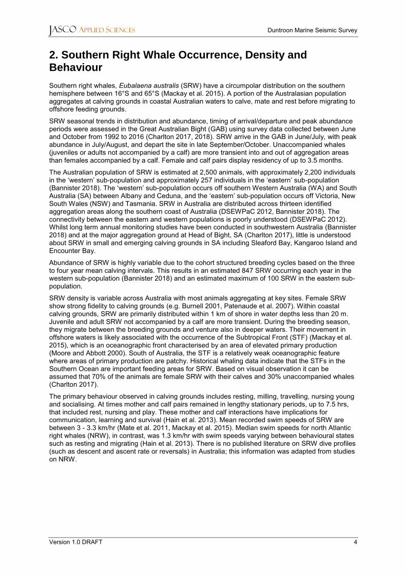
JASCO APPLIED SCIENCES Duntroon Marine Seismic Survey
Version 1.0 DRAFT 4
2. Southern Right Whale Occurrence, Density and Behaviour
Southern right whales, Eubalaena australis (SRW) have a circumpolar distribution on the southern hemisphere between 16°S and 65°S (Mackay et al. 2015). A portion of the Australasian population aggregates at calving grounds in coastal Australian waters to calve, mate and rest before migrating to offshore feeding grounds.
SRW seasonal trends in distribution and abundance, timing of arrival/departure and peak abundance periods were assessed in the Great Australian Bight (GAB) using survey data collected between June and October from 1992 to 2016 (Charlton 2017, 2018). SRW arrive in the GAB in June/July, with peak abundance in July/August, and depart the site in late September/October. Unaccompanied whales (juveniles or adults not accompanied by a calf) are more transient into and out of aggregation areas than females accompanied by a calf. Female and calf pairs display residency of up to 3.5 months.
The Australian population of SRW is estimated at 2,500 animals, with approximately 2,200 individuals in the ‘western’ sub-population and approximately 257 individuals in the ‘eastern’ sub-population (Bannister 2018). The ‘western’ sub-population occurs off southern Western Australia (WA) and South Australia (SA) between Albany and Ceduna, and the ‘eastern’ sub-population occurs off Victoria, New South Wales (NSW) and Tasmania. SRW in Australia are distributed across thirteen identified aggregation areas along the southern coast of Australia (DSEWPaC 2012, Bannister 2018). The connectivity between the eastern and western populations is poorly understood (DSEWPaC 2012). Whilst long term annual monitoring studies have been conducted in southwestern Australia (Bannister 2018) and at the major aggregation ground at Head of Bight, SA (Charlton 2017), little is understood about SRW in small and emerging calving grounds in SA including Sleaford Bay, Kangaroo Island and Encounter Bay.
Abundance of SRW is highly variable due to the cohort structured breeding cycles based on the three to four year mean calving intervals. This results in an estimated 847 SRW occurring each year in the western sub-population (Bannister 2018) and an estimated maximum of 100 SRW in the eastern sub-population.
SRW density is variable across Australia with most animals aggregating at key sites. Female SRW show strong fidelity to calving grounds (e.g. Burnell 2001, Patenaude et al. 2007). Within coastal calving grounds, SRW are primarily distributed within 1 km of shore in water depths less than 20 m. Juvenile and adult SRW not accompanied by a calf are more transient. During the breeding season, they migrate between the breeding grounds and venture also in deeper waters. Their movement in offshore waters is likely associated with the occurrence of the Subtropical Front (STF) (Mackay et al. 2015), which is an oceanographic front characterised by an area of elevated primary production (Moore and Abbott 2000). South of Australia, the STF is a relatively weak oceanographic feature where areas of primary production are patchy. Historical whaling data indicate that the STFs in the Southern Ocean are important feeding areas for SRW. Based on visual observation it can be assumed that 70% of the animals are female SRW with their calves and 30% unaccompanied whales (Charlton 2017).
The primary behaviour observed in calving grounds includes resting, milling, travelling, nursing young and socialising. At times mother and calf pairs remained in lengthy stationary periods, up to 7.5 hrs, that included rest, nursing and play. These mother and calf interactions have implications for communication, learning and survival (Hain et al. 2013). Mean recorded swim speeds of SRW are between 3 - 3.3 km/hr (Mate et al. 2011, Mackay et al. 2015). Median swim speeds for north Atlantic right whales (NRW), in contrast, was 1.3 km/hr with swim speeds varying between behavioural states such as resting and migrating (Hain et al. 2013). There is no published literature on SRW dive profiles (such as descent and ascent rate or reversals) in Australia; this information was adapted from studies on NRW.

JASCO APPLIED SCIENCES Duntroon Marine Seismic Survey
Version 1.0 DRAFT 5
3. Animal Movement and Exposure Modelling
To assess the risk of impacts from exposure, an estimate of received sound levels for the animals in the area during operation of the Project is required. Sound sources move as do animals. The sound fields may be complex, and the sound received by an animal is a function of where the animal is at any given time. To a reasonable approximation, the location of the sound source(s) is known, and acoustic modeling can be used to predict the 3-D sound field. The location and movement of animals within the sound field, however, is unknown. Realistic animal movement within the sound field can be simulated. Repeated random sampling (Monte Carlo method simulating many animals within the operations area) is used to estimate the sound exposure history of the population of simulated animals during the operation.
Monte Carlo methods provide a heuristic approach for determining the probability distribution function (PDF) of complex situations, such as animals moving in a sound field. The probability of an event’s occurrence is determined by the frequency with which it occurs in the simulation. The greater the number of random samples, in this case the more simulated animals (animats), the better the approximation of the PDF. Animats are randomly placed, or seeded, within the simulation boundary at a specified density (animats/km2). Higher densities provide a finer PDF estimate resolution but require more computational resources. To ensure good representation of the PDF, the animat density is set as high as practical allowing for computation time. The animat density is much higher than the real-world density to ensure good representation of the PDF. The resulting PDF is scaled using the real-world density.
Several models for marine mammal movement have been developed (Ellison et al. 1987, Frankel et al. 2002, Houser 2006). These models use an underlying Markov chain to transition from one state to another based on probabilities determined from measured swimming behavior. The parameters may represent simple states, such as the speed or heading of the animal, or complex states, such as likelihood of participating in foraging, play, rest, or travel.
The JASCO Animal Simulation Model Including Noise Exposure (JASMINE) was based on the open-source marine mammal movement and behavior model, 3MB (Houser 2006) and used to predict the exposure of animats (virtual marine mammals) to sound arising from sound sources in simulated representative surveys. Inside JASMINE, the sound source location mimics the movement of the source vessel through the proposed survey pattern (as described in the MSS report). Animats are programmed to behave like the marine animals likely to be present in the survey area (Figure 2). The parameters used for forecasting realistic behaviors (e.g., diving, foraging, surface times, etc.) are determined and interpreted from marine species studies (e.g., tagging studies) where available, or reasonably extrapolated from related species (see Appendix B for a more detailed explanation of JASMINE and Appendix C for the parameters used in modelling marine mammal movement). An individual animat’s modeled sound exposure levels are summed over the total simulation duration, such as 24 hours or the entire simulation, to determine its total received energy. The maximum PK and SPL exposure during the time period is also determined from the exposure history, and both total energy received and maximum PK or SPL are compared to the relevant criteria (Section 4).
JASMINE uses the same animal movement algorithms as the Marine Mammal Movement and Behavior (3MB) model (Houser 2006) but has been extended to be directly compatible with MONM and FWRAM acoustic field predictions, for inclusion of source tracks, and importantly for animats to change behavioral states based on time and space dependent modeled variables such as received levels for aversion behaviour.

JASCO APPLIED SCIENCES Duntroon Marine Seismic Survey
Version 1.0 DRAFT 6
Figure 2. Cartoon of animats in a moving sound field. The acoustic exposure of each animat is determined by where it is in the sound field, and its exposure history is accumulated as the simulation steps through time. In this cartoon the vessel and sound source with its acoustic footprint (highest sound energy levels shown in red/yellow) are moving from right to left, as is the deepest animat. The two upper animats move from left to right. Because the upper and lower animats are far from the source, low levels of sound exposure are expected. The middle animat is nearer the sound source, so its acoustic exposure is expected to be higher than the other two animats, and its highest exposure occurs closest to the sound source at the second time step (t2).
3.1. Behavioural groups
Female SRWs stay with their offspring close to shore in waters not deeper than 20 m. Unaccompanied SRW (juveniles and adults without accompanying calves) are seen in the breeding areas as well as in deeper waters (Figure 3). To account for this distinction in occurrence and habitat use during the breeding season, two separate behavioural groups were modelled:
• A nearshore group representing mother and calf SRW; and
• An offshore group representing the remaining animals.
As the animat modelling can only consider depth contours, and not features such as BIA boundaries, the 20 m contour has been applied as a reasonable approximate for the boundary of the SRW calving BIA. The area modelled for the offshore group was bound by the 20 m depth contour as a minimum and the 5,000 m depth contour to also account for the southward migration of animals in late September and October.

JASCO APPLIED SCIENCES Duntroon Marine Seismic Survey
Version 1.0 DRAFT 7
Figure 3. Map showing the operations area and the animat seeding boundaries. Nearshore SRW animats were seeded between the 20m contour and the coast. Offshore SRW were seeded between the 5000 m contour and the 20 m contour.
3.2. Simulation scenarios
Model simulations were run with animat densities of 0.5 animats/km2 to generate a statistically reliable probability density function for each behavioural group (see Appendix B). This resulted in a total number of animats modelled for the two behavioural groups (nearshore and offshore) of 211,781 and 148,650, respectively. As mother-calf pairs rarely enter either the Spencer Gulf or St. Vincent Gulf, these areas were excluded from seeding. All animats were randomly distributed throughout their respective seeding areas which are defined by their depth ranges (min/max); the aggregation of females and calves in their key calving areas was not taken into account.
The precise geographic delineation between the two Australian SRW sub-populations remains unclear (Mackay et al. 2015). Based on existing survey data, the home range for the eastern subpopulation was considered to stretch from Albany to Ceduna, the western sub-population from Ceduna to the east. The coastline between Albany (WA) to Ceduna (SA) stretches over 1979 km, from Ceduna to Otway (VIC) over 2839 km coastline; excluding the coastline of Spencer Gulf and St. Vincent Gulf reduces this range to 1630 km. Kangaroo Island, with a coastline of 427 km, was included as SRW are reported for this area; this resulted in a combined coastline for the eastern subpopulation of 2057 km. Due to the uncertainly about the delineation between subpopulations, the entire Australian population was considered which inhabits a coastline of 4036 km during the calving season. The coastline considered in the simulation for the offshore scenario covered a coastline segment of 532 km.

JASCO APPLIED SCIENCES Duntroon Marine Seismic Survey
Version 1.0 DRAFT 8
3.3. Exposure estimation method
The predicted number of SRW exposed to sound levels exceeding the criteria is derived by scaling the modelled number of exposed animals from a ‘population’ of virtual SRW (animats) to the real-world situation; the total number of animats (>100,000 replicates per scenario) is put in relation to the estimated number of SRW occurring south of Australia each year (see Appendix C) and subsequently correcting the animat results for the difference in spatial extent between the entire home range of SRW and the coastline covered in this study.

JASCO APPLIED SCIENCES Duntroon Marine Seismic Survey
Version 1.0 DRAFT 9
4. Noise Effect Criteria
Several sound level metrics are commonly used to evaluate noise and its effects on marine life (Appendix A). The period of accumulation associated with SEL is defined, with this report referencing either a “per pulse” assessment or over 24 h. Appropriate subscripts indicate any applied frequency weighting; unweighted SEL is defined as required. The acoustic metrics in this report reflect the updated ANSI and ISO standards for acoustic terminology, ANSI-ASA S1.1 (R2013) and ISO/DIS 18405.2:2017 (2016). The criteria considered in this study are as follows:
1. The noise criteria relevant to the SRW exposure assessment, applied in the modelling study Wladichuk et al. (2018), are as follows: Peak pressure levels (PK; Lpk) and frequency-weighted accumulated sound exposure levels (SEL; LE,24h) from the U.S. National Oceanic and Atmospheric Administration (NOAA) Technical Guidance (NMFS 2018) for the onset of permanent threshold shift (PTS) and temporary threshold shift (TTS) in marine mammals.
2. Marine mammal behavioural threshold based on the current interim U.S. National Marine Fisheries Service (NMFS) criterion (NMFS 2013) for marine mammals of 160 dB re 1 µPa SPL (Lp) for impulsive sound sources.
3. Low-frequency (LF) weighted SPL for comparison to the Wood et al. (2012) probabilistic disturbance thresholds for migrating mysticetes (relevant for calving mysticetes), assessed using the NMFS (2018) frequency weighting function. The relevant thresholds are LF-weighted SPLs of 120, 140 and 160 dB re 1 µPa, relating to response likelihoods of 10, 50 and 90%, respectively.
4.1. Marine mammal weighting functions
The potential for anthropogenic sounds to impact marine mammals is largely dependent on whether the sound occurs at frequencies that an animal can hear well, unless the sound pressure is so high that it can cause physical tissue damage regardless of frequency. For sound levels below such extremes, the importance of sound components at particular frequencies can be scaled by frequency weighting the sound relative to an animal’s sensitivity to those frequencies. Auditory (frequency) weighting functions reflect an animal’s ability to hear a sound (Nedwell and Turnpenny 1998, Nedwell et al. 2007). Auditory weighting functions have been proposed for marine mammals, specifically associated with PTS thresholds expressed in metrics that consider what is known about marine mammal hearing (e.g., SEL) (Southall et al. 2007, Erbe et al. 2016, Finneran 2016). Marine mammal auditory weighting functions published by Finneran (2016) are included in the NMFS 2018 Technical Guidance for use in conjunction with corresponding PTS (injury) onset acoustic criteria (Appendix A.2).
4.2. Behavioural response
Despite numerous studies on marine mammal behavioural responses to sound exposure there is not yet consensus within the scientific community regarding the appropriate metric or sound levels useful for assessing behavioural reactions. It is recognised that the context in which the sound is received affects the nature and extent of responses to a stimulus (Southall et al. 2007, Ellison and Frankel 2012, Southall et al. 2016). Because of the complexity and variability of marine mammal behavioural responses to acoustic exposure, NMFS has not yet released updated technical guidance providing criteria or thresholds for evaluating behavioural disruption (NMFS 2018). The NMFS currently uses a step function to assess behavioural impact. Initially, the probability of inducing behavioural responses at a SPL of 160 dB re 1 µPa was derived from the HESS (1999) report which, in turn, was based on the responses of migrating mysticete whales to airgun sounds (Malme et al. 1983, Malme et al. 1984). The HESS team recognized that behavioural responses to sound may occur at lower levels, but significant responses were only likely to occur above a SPL of 140 dB re 1 µPa. An extensive review of behavioural responses to sound was undertaken by Southall et al. (2007, their Appendix B). Southall et al. (2007) found varying responses for most marine mammals between a SPL of 140 and 180 dB re 1 µPa, consistent with the HESS (1999) report, but lack of convergence in the data prevented them from suggesting explicit step functions. Absence of controls, precise measurements, appropriate metrics, and context dependency of responses (including the activity state of the animal)

JASCO APPLIED SCIENCES Duntroon Marine Seismic Survey
Version 1.0 DRAFT 10
all contribute to variability. For impulsive sounds, this threshold is 160 dB re 1 µPa SPL for cetaceans (NMFS 2013).
Wood et al. (2012) proposed a step function of the probability of response for impulsive sounds using a frequency weighted SPL metric. They defined behavioural response categories for sensitive species (including harbor porpoise and beaked whales) and for migrating mysticetes. The migrating mysticete category has been applied in this analysis to Southern Right Whales, in particular within the calving and calving buffer BIAs, but also during migration, to assess behavioural response to impulsive sounds (Table 1). The Wood et al. (2012) approach has been updated to consider the frequency weighting from NMFS (2018).
Table 1. Behavioural exposure criteria used in this analysis for calving and migrating southern right whales Probability of behavioural response to LF-weighted sound pressure level (SPL dB re 1 µPa) (NMFS (2018). Probabilities are not additive. Adapted from Wood et al. (2012).
Probability of response to frequency-weighted SPL (dB re 1 µPa)
120 140 160
10% 50% 90%
4.3. Injury and hearing sensitivity changes
Exposure to sufficiently intense sound may lead to an increased hearing threshold in any living animal capable of perceiving acoustic stimuli by some means of a sensory receptor. Such an increase in hearing threshold due to noise exposure is called a threshold shift (TS). If this shift is reversed and the hearing threshold returns to normal, the NITS is called a temporary threshold shift (TTS). If the threshold shift does not return to normal, the residual TS is called a permanent threshold shift (PTS).
To assist in assessing the potential for injuries to marine mammals this report applies the criteria recommended by NMFS (2018); both PTS and TTS are considered to help assess the potential for injuries to marine mammals, Table 2. Appendix A provides more information about the NMFS (2018) criteria.
Table 2. The SEL24h (LE,24h) and PK (Lpk) thresholds for acoustic effects on southern right whales. Injury is defined as permanent threshold shift (PTS).
Hearing group
NMFS (2018)
PTS onset thresholds* (received level)
TTS onset thresholds* (received level)
Weighted SEL24h (LE, 24h;
dB re 1 μPa2·s)
PK (Lpk; dB re 1 μPa)
Weighted SEL24h (LE, 24h;
dB re 1 μPa2·s)
PK (Lpk; dB re 1 μPa)
Low-frequency cetaceans
183 219 168 213
* Dual metric acoustic thresholds for impulsive sounds: Use whichever results in the largest isopleth for calculating PTS onset. If a non-impulsive sound has the potential of exceeding the peak sound pressure level thresholds associated with impulsive sounds, these thresholds should also be considered. Lpk, flat–peak sound pressure is flat weighted or unweighted and has a reference value of 1 µPa LE - denotes cumulative sound exposure over a 24-hour period and has a reference value of 1 µPa2s Subscript LF indicates the marine mammal auditory weighting function for low-frequency cetaceans.

JASCO APPLIED SCIENCES Duntroon Marine Seismic Survey
Version 1.0 DRAFT 11
5. Results
This section presents the estimated number of SRW expected to receive sound levels exceeding behavioural and injurious thresholds in a 24 h period.
5.1. Real world exposure estimates
The numbers of modelled animats (Appendix D) exposed to acoustic levels exceeding thresholds must be scaled to relate to the number of SRW in the survey area. Two scaling factors are calculated:
1. A correction factor accounting for the difference in animats compared to the number of SRW in the (sub-)population; and
2. A spatial factor setting the survey area (km coastline) in proportion to the overall home range of SRW during the survey period.
The real-world number of SRW potentially exposed to sound levels exceeding the noise exposure thresholds are given for the two scenarios (nearshore vs offshore) based on numbers of SRW for the entire Australian population (Table 3) and the eastern sub-population (Table 4). The exposures for the eastern population, nearshore SRW, are approximately equivalent to the exposures within the SRW calving BIA.
Table 3. Spatial scaling of animat modelling results for entire SRW population. Scaling number of animat exposed to sound levels exceeding the noise exposure criteria based on coastline including in the animat modelling as compared to home range of SRW for the entire Australian population.
Sub-population Spatial
correction [%]
120 dB (Lp,LF)
140 dB (Lp,LF)
160 dB (Lp,LF)
160 dB (Lp)
TTS
168 dB
(LE, LF, 24h)
PTS†
183 dB
(LE, LF, 24h)
Offshore SRW (males/juveniles)
0.13 5.39 1.15 0.34 0.52 0.41 0.01
Nearshore SRW (females/calves)
0.13 5.15 0 0 0 0 0
Lp,LF – denotes low-frequency weighted sound pressure level and has a reference value of 1 µPa Lp - denotes sound pressure level and has a reference value of 1 µPa LE - denotes cumulative sound exposure over a 24-hour period and has a reference value of 1 µPa2s †The model does not account for shutdowns.
Table 4. Spatial scaling of animat modelling results for eastern SRW population. Scaling number of animat exposed to sound levels exceeding the noise exposure criteria based on coastline including in the animat modelling as compared to home range of SRW for the eastern Australian population.
Sub-population Spatial
correction [%]
120 dB (Lp,LF)
140 dB (Lp,LF)
160 dB (Lp,LF)
160 dB (Lp)
TTS
168 dB
(LE, LF, 24h)
PTS†
183dB
(LE, LF, 24h)
Offshore SRW (males/juveniles)
0.26 1.12 0.24 0.07 0.11 0.09 0.001
Nearshore SRW (females/calves)
0.26 1.07 0 0 0 0 0
Lp,LF – denotes low-frequency weighted sound pressure level and has a reference value of 1 µPa Lp - denotes sound pressure level and has a reference value of 1 µPa LE - denotes cumulative sound exposure over a 24-hour period and has a reference value of 1 µPa2s †The model does not account for shutdowns.

JASCO APPLIED SCIENCES Duntroon Marine Seismic Survey
Version 1.0 DRAFT 12
6. Discussion and Conclusion
The extreme site-fidelity of female SRW during the calving season restricts their movements to areas at large distances (>50 km) from the operational survey area. In addition, female SRW and their calves exhibit a dive behaviour which prevents them from exposure to intense levels of sound due to physical acoustic effects that reduce the sound levels received near the surface. One supposition implicit to animat modelling is that the virtual animals are distributed randomly (i.e., more or less evenly) over areas restricted by bathymetry due to their depth preference.
This is contrary to the aggregated distribution of nearshore SRW in their calving grounds (Bannister 2017). Given that none of the known key calving grounds of SRW along the coastline of South Australia, especially their main grounds at Head of Bight and Fowler’s Bay, is in this area considered in this model, this even distribution of animats results in an overestimation of SRW exposed to the seismic airgun impulses.
The dive parameters chosen in this model had to be partially derived from northern right whales. The chosen parameters result in a variation of types of dive behaviour which resemble the behaviour described from visual observations of SRW in their calving grounds. Changes to the dive depth, duration and profile are individually different, highly complex and depend on behavioural context, gender, motivation and numerous other biological parameters. Updated information on SRW behaviour will allow improving the precision of the modelling results in the future, but substantial changes to the results are unlikely unless completely unexpected dive behaviour is discovered.
Scaling the modelling results to the real-world situation based on the entire Australian population size represents an overestimation of the number of affected SRW as the survey area is closest to areas inhabited by the eastern SRW sub-population which occurs at lower densities and represents approximately only 1/9th of the entire SRW population. This ratio can change depending on the number of animals ‘seeded’ in each of the sub-populations.
The proportion – in relation to the overall population of Australian SRW – of animals returning to south Australian waters each year can only be estimated and is variable. A count for the western sub-population resulted in 847 SRW (Bannister 2018) while the eastern can only be stimated; a ratio of 1:3 to 1:4 relative to the overall population size can be assumed (C.Charlton, pers. Comm; (Charlton 2017). In this analysis, a ratio of 3 was used as a conservative approach, resulting in an estimated 100 SRW for the eastern area. Based on an estimate of 300 SRW for the eastern sub-population and by applying a ratio of, e.g., 3.94 (Bannister 2017)1, the resulting eastern number of animals belonging to the eastern sub-population would be 76 animals instead of 100. Accordingly, the modelling results for this sub-population most likely represent an overestimation by 33%.
Offshore SRW (unaccompanied adults and juveniles) have a higher predicted likelihood of exposure to sound levels above the threshold criteria than SRW in the nearshore areas (females and calves). In this model, a 70/30 ratio has been used, but this may underestimate the number of animals in the offshore region; assuming a higher number of SRW occurring in offshore waters south of Australia (e.g., choosing a 50/50 ratio) would increase the number of animals exposed to levels beyond the threshold for a 10% response likelihood slightly (resulting in an increase by 3 SRW for the entire population, <1 SRW for the eastern population); the other effect categories would change only marginally (e.g. increase <0.2 SRW).
The animat model assumes a uniformly (random) distribution of animats along the coastline. SRW, however, occur in the BIA in aggregations in their calving grounds which are distant (>50 km) from the survey area. Apart from animals migrating between calving grounds, nearshore SRW are not likely to be present in the BIA between those calving grounds. The area exposed to LF-weighted sound levels >120 dB re 1 µPa (SPL) covers a zone within the BIA that does not contain one of known calving SRW grounds including the emerging Sleaford Bay area. Accordingly, the number of SRW predicted to be exposed to sound levels exceeding the threshold for a 10% response likelihood is most likely an overestimation. In an example from the closest single impulse to the coast (Figure 4), also shown focused on the coastline (Figure 5), this zone stretches over 24.9 km and 1,307 animats were seeded
1 The current population size of SRW is is estimated using a model, whereby the cow/calf count over three years (to allow for the 3-year periodicity in calving) is multiplied by a factor of 3.94.

JASCO APPLIED SCIENCES Duntroon Marine Seismic Survey
Version 1.0 DRAFT 13
in this area. By scaling this number down to the real-world situation, a total of four (3.89) SRW would be predicted to be exposed – as compared to up to five (5.39) SRW predicted to be exposed by looking at the entire population and one (1.12) SRW if only considering the eastern population. In this context it is important to note that none of the known key aggregation areas is located within this zone which reduces the risk of SRW of being exposed to LF-weighted sound levels >120 dB re 1 µPa (SPL) substantially.
It is evident that SRW will start migrating south at the end of the calving season, but it remains unclear if there are migratory corridors or if animals are moving south from wherever they roamed prior to the start of the migration. A relatively large proportion of SRW is present in aggregation areas in SA (Fowler Bay and Head of Bight) north of the operational area. A southward movement from there would take animals close to the operational area with an increased the risk of exposure to higher sound levels. Due to compete lack of information on this aspect, it is impossible to assess if the modelling results are biased toward an under- or overestimation of numbers.
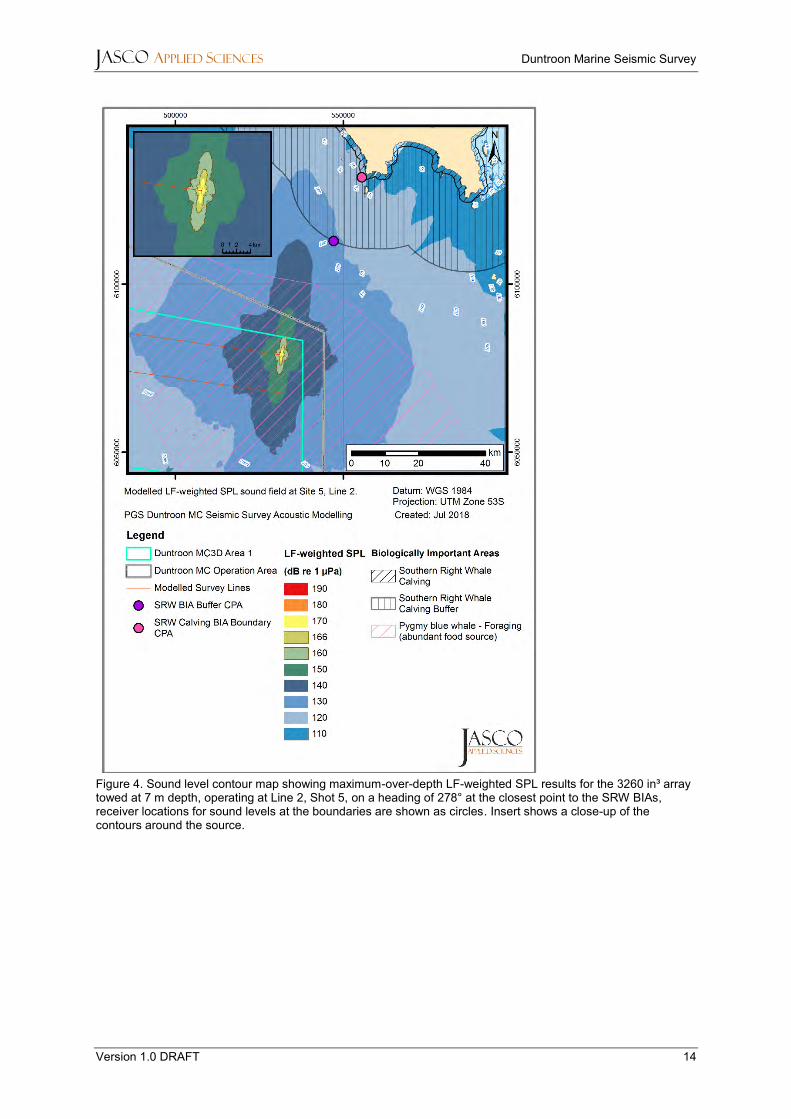
JASCO APPLIED SCIENCES Duntroon Marine Seismic Survey
Version 1.0 DRAFT 14
Figure 4. Sound level contour map showing maximum-over-depth LF-weighted SPL results for the 3260 in³ array towed at 7 m depth, operating at Line 2, Shot 5, on a heading of 278° at the closest point to the SRW BIAs, receiver locations for sound levels at the boundaries are shown as circles. Insert shows a close-up of the contours around the source.
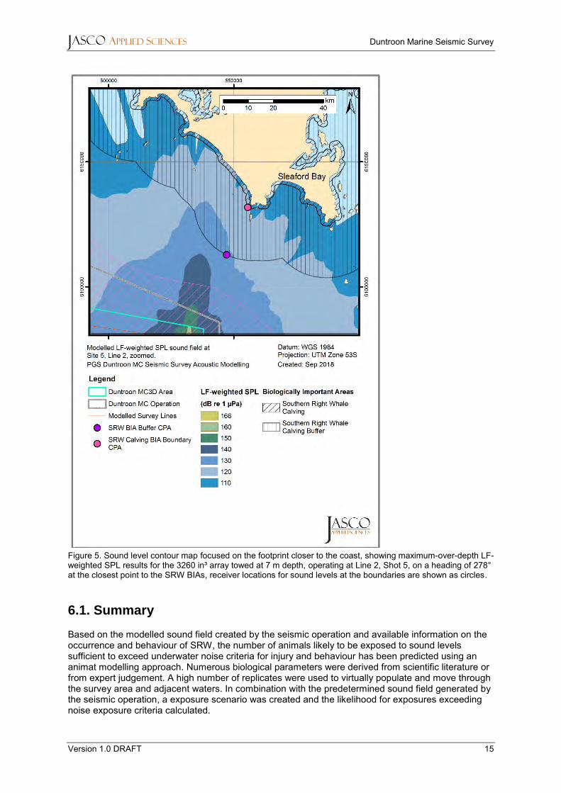
JASCO APPLIED SCIENCES Duntroon Marine Seismic Survey
Version 1.0 DRAFT 15
Figure 5. Sound level contour map focused on the footprint closer to the coast, showing maximum-over-depth LF-weighted SPL results for the 3260 in³ array towed at 7 m depth, operating at Line 2, Shot 5, on a heading of 278° at the closest point to the SRW BIAs, receiver locations for sound levels at the boundaries are shown as circles.
6.1. Summary
Based on the modelled sound field created by the seismic operation and available information on the occurrence and behaviour of SRW, the number of animals likely to be exposed to sound levels sufficient to exceed underwater noise criteria for injury and behaviour has been predicted using an animat modelling approach. Numerous biological parameters were derived from scientific literature or from expert judgement. A high number of replicates were used to virtually populate and move through the survey area and adjacent waters. In combination with the predetermined sound field generated by the seismic operation, a exposure scenario was created and the likelihood for exposures exceeding noise exposure criteria calculated.

JASCO APPLIED SCIENCES Duntroon Marine Seismic Survey
Version 1.0 DRAFT 16
The modelling results indicate that the proposed seismic operation will likely have behavioural effects (i.e. 10% response likelihood) on a small number of SRW (1 of the eastern sub-population or 5 relative to the entire SRW population present per year, Table 5). The likelihood of causing an increased behavioural response or injurious effects is increasingly smaller (>1 SRW, Table 6) and erroneously inflated by the model assumption of an even distribution of SRW along the coastline.
Table 5. Predicted, scaled number of animat exposed to sound pressure levels exceeding behavioural disturbance criteria for eastern and entire SRW (sub-)population during the 24 h simulation.
(Sub-) Population
Eastern Entire
Adapted from Wood et al. (2012)
NMFS (2013) Adapted from Wood et al. (2012) NMFS (2013)
120 dB (Lp,LF)
140 dB (Lp,LF)
160 dB (Lp,LF)
160 dB (Lp) 120 dB (Lp,LF)
140 dB (Lp,LF)
160 dB (Lp,LF)
160 dB (Lp)
Offshore SRW (males/juveniles)
1.12 0.24 0.07 0.11 5.39 1.15 0.34 0.52
Nearshore SRW (females/calves)
1.07 0 0 0 0 0 0
Lp,LF – denotes low-frequency weighted sound pressure level and has a reference value of 1 µPa Lp - denotes sound pressure level and has a reference value of 1 µPa
Table 6. Predicted, scaled number of animat exposed to sound exposure levels exceeding the TTS and PTS criteria from NMFS (2018) for entire and eastern SRW (sub-)population during the 24 h simulation.
(Sub-) Population
Eastern Entire
TTS
168 dB re 1 μPa2·s
(LE, LF, 24h)
PTS†
183 dB re 1 μPa2·s
(LE, LF, 24h)
TTS
168 dB re 1 μPa2·s
(LE, LF, 24h)
PTS†
183 dB re 1 μPa2·s
(LE, LF, 24h)
Offshore SRW (males/juveniles)
0.09 0.001 0.41 0.01
Nearshore SRW (females/calves)
0 0 0 0
†The model does not account for shutdowns.

JASCO APPLIED SCIENCES Duntroon Marine Seismic Survey
Version 1.0 DRAFT 17
Glossary
3-D
Three-dimensional
1/3-octave-band
Non-overlapping passbands that are one-third of an octave wide (where an octave is a doubling of frequency). Three adjacent 1/3-octave-bands comprise a one octave-band. One-third-octave-bands become wider with increasing frequency. Also see octave.
audiogram
A graph of hearing threshold level (sound pressure levels) as a function of frequency, which describes the hearing sensitivity of an animal over its hearing range.
auditory weighting function (frequency-weighting function)
Auditory weighting functions account for marine mammal hearing sensitivity. They are applied to sound measurements to emphasise frequencies that an animal hears well and de-emphasise frequencies they hear less well or not at all (Southall et al. 2007, Finneran and Jenkins 2012, NOAA 2013).
bandwidth
The range of frequencies over which a sound occurs. Broadband refers to a source that produces sound over a broad range of frequencies (e.g., seismic airguns, vessels) whereas narrowband sources produce sounds over a narrow frequency range (e.g., sonar) (ANSI/ASA S1.13-2005 R2010).
BIA
Biologically Important Area (http://www.environment.gov.au/marine/marine-species/bias)
cetacean
Any animal in the order Cetacea. These are aquatic, mostly marine mammals and include whales, dolphins, and porpoises.
decibel (dB)
One-tenth of a bel. Unit of level when the base of the logarithm is the tenth root of ten, and the quantities concerned are proportional to power (ANSI S1.1-1994 R2004).
ensonified area
The total area ensonified in conjunction with a specified isopleth.
frequency
The rate of oscillation of a periodic function measured in cycles-per-unit-time. The reciprocal of the period. Unit: hertz (Hz). Symbol: f. 1 Hz is equal to 1 cycle per second.
functional hearing group
Grouping of marine mammal species with similar estimated hearing ranges. Southall et al. (2007) proposed the following functional hearing groups: low-, mid-, and high-frequency cetaceans, pinnipeds in water, and pinnipeds in air.
GAB Great Australian Bight
hearing threshold
The sound pressure level that is barely audible for a given individual in the absence of significant background noise during a specific percentage of experimental trials.
hertz (Hz)
A unit of frequency defined as one cycle per second.

JASCO APPLIED SCIENCES Duntroon Marine Seismic Survey
Version 1.0 DRAFT 18
impulsive sound
Sound that is typically brief and intermittent with rapid (within a few seconds) rise time and decay back to ambient levels (NOAA 2013, ANSI S12.7-1986 R2006). For example, seismic airguns and impact pile driving.
low-frequency cetacean
The functional hearing group that represents mysticetes (baleen whales).
MC
Multi-Client
MSS
Marine Seismic Survey
mysticete
Mysticeti, a suborder of cetaceans, use their baleen plates, rather than teeth, to filter food from water. They are not known to echolocate but use sound for communication. Members of this group include rorquals (Balaenopteridae), right whales (Balaenidae), and the grey whale (Eschrichtius robustus).
octave
The interval between a sound and another sound with double or half the frequency. For example, one octave above 200 Hz is 400 Hz, and one octave below 200 Hz is 100 Hz.
peak pressure level (PK)
The maximum instantaneous sound pressure level, in a stated frequency band, within a stated period. Also called zero-to-peak pressure level. Unit: decibel (dB).
peak-to-peak pressure level (PK-PK)
The difference between the maximum and minimum instantaneous pressure levels. Unit: decibel (dB).
permanent threshold shift (PTS)
A permanent loss of hearing sensitivity caused by excessive noise exposure. PTS is considered auditory injury.
pressure, acoustic
The deviation from the ambient hydrostatic pressure caused by a sound wave. Also called overpressure. Unit: pascal (Pa). Symbol: p.
pulsed sound
Discrete sounds with durations less than a few seconds. Sounds with longer durations are called continuous sounds.
received level
The sound level measured at a receiver.
signature
Pressure signal generated by a source.
sound
A time-varying pressure disturbance generated by mechanical vibration waves travelling through a fluid medium such as air or water.
sound exposure
Time integral of squared, instantaneous frequency-weighted sound pressure over a stated time interval or event. Unit: pascal-squared second (Pa2·s) (ANSI S1.1-1994 R2004).

JASCO APPLIED SCIENCES Duntroon Marine Seismic Survey
Version 1.0 DRAFT 19
sound exposure level (SEL)
A cumulative measure related to the sound energy in one or more pulses. Unit: dB re 1 µPa2·s. SEL is expressed over the summation period (e.g., per-pulse SEL [for airguns], single-strike SEL [for pile drivers], 24-hour SEL).
sound field
Region containing sound waves (ANSI S1.1-1994 R2004).
sound pressure level (SPL)
The decibel ratio of the time-mean-square sound pressure, in a stated frequency band, to the square of the reference sound pressure (ANSI S1.1-1994 R2004).
For sound in water, the reference sound pressure is one micropascal (p0 = 1 µPa) and the unit for SPL is dB re 1 µPa:
( ) ( )010
2
0
2
10 /log20/log10SPL pppp ==
Unless otherwise stated, SPL refers to the root-mean-square sound pressure level. See also 90% sound pressure level and fast-average sound pressure level. Non-rectangular time window functions may be applied during calculation of the rms value, in which case the SPL unit should identify the window type.
sound speed profile
The speed of sound in the water column as a function of depth below the water surface.
source level (SL)
The sound pressure level or sound exposure level measured 1 metre from a theoretical point source that radiates the same total sound power as the actual source. Unit: dB re 1 μPa2m2 or dB 1 μPa2m2s.
spectrum
An acoustic signal represented in terms of its power (or energy) distribution versus frequency.
temporary threshold shift (TTS)
Temporary loss of hearing sensitivity caused by excessive noise exposure.
transmission loss (TL)
Also called propagation loss, this refers to the decibel reduction in sound level between two stated points that results from sound spreading away from an acoustic source subject to the influence of the surrounding environment.
wavelength
Distance over which a wave completes one oscillation cycle. Unit: meter (m). Symbol: λ.

JASCO APPLIED SCIENCES Duntroon Marine Seismic Survey
Version 1.0 DRAFT 20
Literature Cited
[DEWHA] Department of the Environment, W., Heritage and the Arts. 2008. EPBC Act Policy Statement 2.1 - Interaction Between Offshore Seismic Exploration and Whales. In: Department of the Environment, W., Heritage and the Arts. 14 pp.
[HESS] High Energy Seismic Survey. 1999. High Energy Seismic Survey Review Process and Interim Operational Guidelines for Marine Surveys Offshore Southern California. Prepared for the California State Lands Commission and the United States Minerals Management Service Pacific Outer Continental Shelf Region by the High Energy Seismic Survey Team, Camarillo, California. 98 pp.
[ISO] International Organization for Standardization. 2016. ISO/DIS 18405.2:2017. Underwater acoustics—Terminology. Geneva. https://www.iso.org/standard/62406.html.
[NMFS] National Marine Fisheries Service. 1998. Acoustic Criteria Workshop. Dr. Roger Gentry and Dr. Jeanette Thomas Co-Chairs.
[NMFS] National Marine Fisheries Service. 2013. Marine Mammals: Interim Sound Threshold Guidance (webpage). National Marine Fisheries Service, National Oceanic and Atmospheric Administration, U.S. Department of Commerce. http://www.westcoast.fisheries.noaa.gov/protected_species/marine_mammals/threshold_guidance.html.
[NMFS] National Marine Fisheries Service. 2018. 2018 Revision to: Technical Guidance for Assessing the Effects of Anthropogenic Sound on Marine Mammal Hearing (Version 2.0): Underwater Thresholds for Onset of Permanent and Temporary Threshold Shifts. U.S. Department of Commerce, NOAA. NOAA Technical Memorandum NMFS-OPR-59, Silver Spring, MD. 167 pp. https://www.fisheries.noaa.gov/webdam/download/75962998.
[NOAA] National Oceanic and Atmospheric Administration. 2013. Draft guidance for assessing the effects of anthropogenic sound on marine mammals: Acoustic threshold levels for onset of permanent and temporary threshold shifts, December 2013, 76 pp. Silver Spring, Maryland: NMFS Office of Protected Resources. http://www.nmfs.noaa.gov/pr/acoustics/draft_acoustic_guidance_2013.pdf.
[NOAA] National Oceanic and Atmospheric Administration. 2015. Draft guidance for assessing the effects of anthropogenic sound on marine mammal hearing: Underwater acoustic threshold levels for onset of permanent and temporary threshold shifts, July 2015, 180 pp. Silver Spring, Maryland: NMFS Office of Protected Resources. http://www.nmfs.noaa.gov/pr/acoustics/draft%20acoustic%20guidance%20July%202015.pdf.
[NOAA] National Oceanic and Atmospheric Administration. 2016. Document Containing Proposed Changes to the NOAA Draft Guidance for Assessing the Effects of Anthropogenic Sound on Marine Mammal Hearing: Underwater Acoustic Threshold Levels for Onset of Permanent and Temporary Threshold Shifts, p. 24. http://www.nmfs.noaa.gov/pr/acoustics/draft_guidance_march_2016_.pdf.
[ONR] Office of Naval Research. 1998. ONR Workshop on the Effect of Anthropogenic Noise in the Marine Environment. Dr. R. Gisiner Chair.
ANSI S12.7-1986. R2006. American National Standard Methods for Measurements of Impulsive Noise. American National Standards Institute, New York.
ANSI S1.1-1994. R2004. American National Standard Acoustical Terminology. American National Standards Institute, New York.
ANSI S1.1-2013. R2013. American National Standard Acoustical Terminology. American National Standards Institute, New York.

JASCO APPLIED SCIENCES Duntroon Marine Seismic Survey
Version 1.0 DRAFT 21
ANSI/ASA S1.13-2005. R2010. American National Standard Measurement of Sound Pressure Levels in Air. American National Standards Institute and Acoustical Society of America, New York.
Bannister, J.L. 2017. Project A7- Monitoring Population Dynamics of ‘Western’ Right Whales off Southern Australia 2015-2018. Final report. National Environment Science Program, Australian Commonwealth Government.
Bannister, J.L. 2018. Monitoring Population Dynamics of ‘Western’ Right Whales off Southern Australia 2015-2018 – Final Report on activities for 2017. National Environmental Science Programme, Marine Biodiversity Hub. Western Australian Museum (lead organisation).
Baumgartner, M.F. and B.R. Mate. 2003. Summertime foraging ecology of North Atlantic right whales. Marine Ecology Progress Series 264: 123-135.
Baumgartner, M.F. and B.R. Mate. 2005. Summer and fall habitat of North Atlantic right whales (Eubalaena glacialis) inferred from satellite telemetry. Canadian Journal of Fisheries and Aquatic Sciences 62(3): 527-543.
Burnell, S.R. 2001. Aspects of the reproductive biology, movements and site fidelity of right whales off Australia. Journal of Cetacean Research and Management (Special Issue 2): 89-102.
Charlton, C.M. 2017. Population demographics of southern right whales (Eubalaena australis) in Southern Australia. PhD Thesis. Curtin University, Western Australia
Charlton, C.M. 2018. Southern right whale distribution, abundance, density and behaviour in the Great Australian Bight. Centre for Marine Science and Technology, Curtin University Western Australia and
Green Light Environmental, Fremantle, Perth, Western Australia. 6 pp.
DSEWPaC. 2012. Conservation Management Plan for the Southern Right Whale: A Recovery Plan under the Environment
Protection and Biodiversity Conservation Act 1999 (2011–2021). In: Department of Sustainability, E., Water, Population and Communities; Australian Department of Environment.
Ellison, W.T., C.W. Clark, and G.C. Bishop. 1987. Potential use of surface reverberation by bowhead whales, Balaena mysticetus, in under-ice navigation: Preliminary considerations. Report of the International Whaling Commission. Volume 37. 329-332 pp.
Ellison, W.T. and P.J. Stein. 1999. SURTASS LFA High Frequency Marine Mammal Monitoring (HF/M3) Sonar: Sustem Description and Test & Evaluation. Under U.S. Navy Contract N66604-98-D-5725.
Ellison, W.T. and A.S. Frankel. 2012. A common sense approach to source metrics. In Popper, A.N. and A. Hawkins (eds.). The Effects of Noise on Aquatic Life. Springer. pp 433-438.
Erbe, C., R. McCauley, and A. Gavrilov. 2016. Characterizing marine soundscapes. In Popper, N.A. and A. Hawkins (eds.). The Effects of Noise on Aquatic Life II. Springer New York, New York, NY. pp 265-271. http://dx.doi.org/10.1007/978-1-4939-2981-8_31.
Finneran, J.J. and C.E. Schlundt. 2010. Frequency-dependent and longitudinal changes in noise-induced hearing loss in a bottlenose dolphin (Tursiops truncatus). Journal of the Acoustical Society of America 128(2): 567-570.
Finneran, J.J. and A.K. Jenkins. 2012. Criteria and thresholds for U.S. Navy acoustic and explosive effects analysis. SPAWAR Systems Center Pacific, San Diego, California.
Finneran, J.J. 2015. Auditory weighting functions and TTS/PTS exposure functions for cetaceans and marine carnivores. San Diego: SSC Pacific.

JASCO APPLIED SCIENCES Duntroon Marine Seismic Survey
Version 1.0 DRAFT 22
Finneran, J.J. 2016. Auditory weighting functions and TTS/PTS exposure functions for marine mammals exposed to underwater noise. Technical Report. 49 pp.
Frankel, A.S., W.T. Ellison, and J. Buchanan. 2002. Application of the acoustic integration model (AIM) to predict and minimize environmental impacts. OCEANS'02 MTS/IEEE. pp 1438-1443.
Hain, J.H.W., J.D. Hampp, S.A. McKenney, J.A. Albert, and R.D. Kenney. 2013. Swim Speed, Behavior, and Movement of North Atlantic Right Whales (Eubalaena glacialis) in Coastal Waters of Northeastern Florida, USA. PLOS ONE 8(1): e54340. https://doi.org/10.1371/journal.pone.0054340.
Houser, D.S. and M.J. Cross. 1999. Marine Mammal Movement and Behavior (3MB): A Component of the Effects of Sound on the Marine Environment (ESME) Distributed Model. Version 8.08, by BIOMIMETICA.
Houser, D.S. 2006. A method for modeling marine mammal movement and behavior for environmental impact assessment. IEEE Journal of Oceanic Engineering 31(1): 76-81.
Kenney, R.D. 2009. Right whales. In Perrin, W.F., B. Wuersig, and J.G.M. Thewissen (eds.). Encyclopedia of marine mammals. 2 edition. Academic Press, Burlington. pp 962-972.
Lucke, K., U. Siebert, P. Lepper, A., and M.-A. Blanchet. 2009. Temporary shift in masked hearing thresholds in a harbor porpoise (Phocoena phocoena) after exposure to seismic airgun stimuli. Journal of the Acoustical Society of America 125(6): 4060-4070.
Mackay, A.I., F. Bailleul, S. Childerhouse, D. Donnelly, R. Harcourt, P. G.J., and S.D. Goldsworthy. 2015. Offshore migratory movement of southern right whales: addressing critical conservation and management needs. SARDI Research Report Series. Document Number F2015/000526-1. South Australian Research and Development Institute (Aquatic Sciences), Adelaide. 40 pp.
Malme, C.I., P.R. Miles, C.W. Clark, P. Tyak, and J.E. Bird. 1983. Investigations of the Potential Effects of Underwater Noise from Petroleum Industry Activities on Migrating Gray Whale Behavior. Report Number 5366. http://www.boem.gov/BOEM-Newsroom/Library/Publications/1983/rpt5366.aspx.
Malme, C.I., P.R. Miles, C.W. Clark, P. Tyack, and J.E. Bird. 1984. Investigations of the potential effects of underwater noise from petroleum industry activities on migrating gray whale behavior. Phase II: January 1984 migration. Report Number BBN Report 5586. Bolt Beranek and Newman Inc. 357 pp.
Mate, B.R., P.B. Best, B.A. Lagerquist, and M.H. Winsor. 2011. Coastal, offshore and migratory movements of South African right whales revealed by satellite telemetry. Marine Mammal Science 27(3): 455-476.
Mellinger, D.K., S.L. Nieukirk, H. Matsumoto, S.L. Heimlich, R.P. Dziak, J. Haxel, M. Fowler, C. Meinig, and H.V. Miller. 2007. Seasonal occurence of North Atlantic right whale (Eubalaena glacialis) vocalizations at two sites on the scotian shelf. Marine Mammal Science 23(4): 856-867.
Moore, J.K. and M.R. Abbott. 2000. Phytoplankton chlorophyll distributions and primary production in the Southern Ocean. Journal of Geophysical Research - Oceans 105(C12): 28709-28722.
Nedwell, J.R. and A.W. Turnpenny. 1998. The use of a generic frequency weighting scale in estimating environmental effect. Workshop on Seismics and Marine Mammals. 23–25th June 1998, London, U.K.
Nedwell, J.R., A.W.H. Turnpenny, J. Lovell, S.J. Parvin, R. Workman, and J.A.L. Spinks. 2007. A validation of the dBht as a measure of the behavioural and auditory effects of underwater noise. Report No. 534R1231 prepared by Subacoustech Ltd. for the UK Department of

JASCO APPLIED SCIENCES Duntroon Marine Seismic Survey
Version 1.0 DRAFT 23
Business, Enterprise and Regulatory Reform under Project No. RDCZ/011/0004. www.subacoustech.com/information/downloads/reports/534R1231.pdf.
Patenaude, N.J., V.A. Portway, C.M. Schaeff, and J.L. Bannister. 2007. Mitochondrial DNA Diversity and Population Structure among Southern Right Whales (Eubalaena australis). Journal of Heredity 98(2): 147-157.
Payne, R. and D. Webb. 1971. Orientation by means of long range acoustic signaling in baleen whales. Annals of the New York Academy of Sciences 188: 110-142.
Southall, B.L., A.E. Bowles, W.T. Ellison, J.J. Finneran, R.L. Gentry, C.R. Greene, Jr., D. Kastak, D.R. Ketten, J.H. Miller, et al. 2007. Marine mammal noise exposure criteria: Initial scientific recommendations. Aquatic Mammals 33(4): 411-521.
Southall, B.L., D.P. Nowaceck, P.J.O. Miller, and P.L. Tyack. 2016. Experimental field studies to measure behavioral responses of cetaceans to sonar. Endangered Species Research 31: 293-315. https://research-repository.st-andrews.ac.uk/bitstream/handle/10023/9942/Miller_2016_ESR_CetaceansToSonar_CC.pdf?sequence=1&isAllowed=y.
Winn, H.E., C.A. Price, and P.W. Sorensen. 1986. The distributional ecology of the right whale Eubalaena glacialis in the western North Atlantic. International Whaling Commission. 129-138 pp.
Wladichuk, J., C. McPherson, K. Lucke, and Z. Li. 2018. Duntroon Marine Seismic Survey: Acoustic Modelling for Assessing Marine Fauna Sound Exposures for a 3260 in³ array. Document Number 01629, Version 1.0. Technical report by JASCO Applied Sciences for PGS Australia.
Wood, J., B.L. Southall, and D.J. Tollit. 2012. PG&E offshore 3 D Seismic Survey Project EIR-Marine Mammal Technical Draft Report. SMRU Ltd.

JASCO APPLIED SCIENCES Duntroon Marine Seismic Survey
Version 1.0 DRAFT A-1
Appendix A. Acoustic Metrics
Underwater sound pressure amplitude is measured in decibels (dB) relative to a fixed reference pressure of p0 = 1 μPa. Because the perceived loudness of sound, especially impulsive noise such as from seismic airguns, pile driving, and sonar, is not generally proportional to the instantaneous acoustic pressure, several sound level metrics are commonly used to evaluate noise and its effects on marine life. We provide specific definitions of relevant metrics used in the accompanying report. Where possible we follow the ANSI and ISO standard definitions and symbols for sound metrics, but these standards are not always consistent.
The zero-to-peak sound pressure level (PK; Lpk; Lp,pk; dB re 1 µPa), is the maximum instantaneous sound pressure level in a stated frequency band attained by an acoustic pressure signal, p(t):
(A-1)
PK is often included as a criterion for assessing whether a sound is potentially injurious; however, because it does not account for the duration of a noise event, it is generally a poor indicator of perceived loudness.
The peak-to-peak sound pressure level (PK-PK; Lpk-pk; Lp,pk-pk; dB re 1 µPa) is the difference between the maximum and minimum instantaneous sound pressure levels in a stated frequency band attained by an impulsive sound, p(t):
(A-2)
The sound pressure level (SPL; Lp; dB re 1 µPa) is the rms pressure level in a stated frequency band over a specified time window (T, s) containing the acoustic event of interest. It is important to note that SPL always refers to an rms pressure level and therefore not instantaneous pressure:
(A-3)
where g(t) is an optional time weighting function. The SPL represents a nominal effective continuous sound over the duration of an acoustic event, such as the emission of one acoustic pulse, a marine mammal vocalisation, the passage of a vessel, or over a fixed duration. Because the window length, T, is the divisor, events with similar sound exposure level (SEL) but more spread out in time have a lower SPL.
In studies of impulsive noise, the time window function g(t) is often a decaying exponential that emphasizes more recent pressure signals to mimic the leaky integration of the mammalian hearing system. For example, human-based fast time weighting applies an exponential function with time constant 125 ms. Another approach for evaluating Lp of impulsive signals is to set T to the “90% time window” (T90): the period over which cumulative square pressure function passes between 5% and 95% of its full per-pulse value. The SPL computed over this T90 interval is commonly called the 90% SPL (SPL(T90); Lp90; dB re 1 µPa):
(A-4)
( )( )
=
0
10,
maxlog20
p
tpL pkp
( ) ( )
−
=− 2
0
2
10,
)(min)(maxlog10
p
tptpL pkpkp
=
2
0
2
10 )(1
log10 pdttpT
LT
p
=
2
0
2
90
1090
90
)(1
log10 pdttpT
LT
p

JASCO APPLIED SCIENCES Duntroon Marine Seismic Survey
Version 1.0 DRAFT A-2
The sound exposure level (SEL; LE; LE,p; dB re 1 µPa2·s) is a measure related to the acoustic energy contained in one or more acoustic events (N). The SEL for a single event is computed from the time-integral of the squared pressure over the full event duration (T):
(A-5)
where T0 is a reference time interval of 1 s. The SEL continues to increase with time when non-zero pressure signals are present. It therefore can be construed as a dose-type measurement, so the integration time used must be carefully considered in terms of relevance for impact to the exposed recipients.
SEL can be calculated over periods with multiple acoustic events or over a fixed duration. For a fixed duration, the square pressure is integrated over the duration of interest. For multiple events, the SEL can be computed by summing (in linear units) the SEL of the N individual events:
. (A-6)
To compute the SPL(T90) and SEL of acoustic events in the presence of high levels of background noise, equations A-4 and A-5 are modified to subtract the background noise contribution:
(A-7)
(A-8)
where is the mean square pressure of the background noise, generally computed by averaging the squared pressure of a temporally-proximal segment of the acoustic recording during which acoustic events are absent (e.g., between pulses).
Because the SPL(T90) and SEL are both computed from the integral of square pressure, these metrics are related by the following expression, which depends only on the duration of the time window T:
(A-9)
(A-10)
where the 0.458 dB factor accounts for the 10% of SEL missing from the SPL(T90) integration time window.
If applied, the frequency weighting of an acoustic event should be specified, as in the case of LF-weighted SEL (e.g., LE,LF,24h; Appendix A.2). The use of fast, slow, or impulse exponential-time-averaging or other time-related characteristics should else be specified.
A.1. Marine Mammal Impact Criteria
Marine mammals can be adversely affected by underwater anthropogenic noise. Payne and Webb (1971) suggested that communication distances of fin whales are reduced by shipping sounds. Subsequently, similar concerns arose regarding effects of other underwater noise sources and the possibility that impulsive sources—primarily airguns used in seismic surveys—could cause auditory injury. This led to a series of workshops held in the late 1990s, conducted to address acoustic mitigation requirements for seismic surveys and other underwater noise sources (NMFS 1998, ONR
=
2
00
2
10 )(log10 pTdttpLT
E
=
=
N
i
NE
iE
L1
10
L
10,
,
10log10
−=
2
0
22
90
1090
90
))((1
log10 pdtntpT
LT
p
−=
2
00
22
10 ))((log10 pTdtntpLT
E
2n
( )TLL Ep 10log10−=
( ) 458.0log10 901090 −−= TLL Ep

JASCO APPLIED SCIENCES Duntroon Marine Seismic Survey
Version 1.0 DRAFT A-3
1998, Nedwell and Turnpenny 1998, HESS 1999, Ellison and Stein 1999). In the years since these early workshops, a variety of thresholds have been proposed for both injury) and disturbance (Section 4.2). The following sections summarise the recent development of thresholds; however, this field remains an active research topic.
A.1.1. Injury In recognition of shortcomings of the SPL-only based injury criteria, in 2005 NMFS sponsored the Noise Criteria Group to review literature on marine mammal hearing to propose new noise exposure criteria. Some members of this expert group published a landmark paper (Southall et al. 2007) that suggested assessment methods similar to those applied for humans. The resulting recommendations introduced dual acoustic injury criteria for impulsive sounds that included peak pressure level thresholds and SEL24h thresholds, where the subscripted 24h refers to the accumulation period for calculating SEL. The peak pressure level criterion is not frequency weighted whereas the SEL24h is frequency weighted according to one of four marine mammal species hearing groups: Low-, Mid- and High-Frequency cetaceans (LF, MF, and HF respectively) and Pinnipeds in Water (PINN). These weighting functions are referred to as M-weighting filters (analogous to the A-weighting filter for human; Appendix A.2). The SEL24h thresholds were obtained by extrapolating measurements of onset levels of Temporary Threshold Shift (TTS) in belugas by the amount of TTS required to produce Permanent Threshold Shift (PTS) in chinchillas. The Southall et al. (2007) recommendations do not specify an exchange rate, which suggests that the thresholds are the same regardless of the duration of exposure (i.e., it implies a 3 dB exchange rate).
Wood et al. (2012) refined Southall et al.’s (2007) thresholds, suggesting lower injury values for LF and HF cetaceans while retaining the filter shapes. Their revised thresholds were based on TTS-onset levels in harbour porpoises from Lucke et al. (2009), which led to a revised impulsive sound PTS threshold for HF cetaceans of 179 dB re 1 µPa2·s. Because there were no data available for baleen whales, Wood et al. (2012) based their recommendations for LF on results obtained from MF studies. In particular they referenced Finneran and Schlundt (2010) research, which found mid-frequency cetaceans are more sensitive to non-impulsive sound exposure than Southall et al. (2007) assumed. Wood et al. (2012) thus recommended a more conservative TTS-onset level for LF cetaceans of 192 dB re 1 µPa2·s.
As of 2017, an optimal approach is not apparent. There is consensus in the research community that an SEL-based method is preferable either separately or in addition to an SPL-based approach to assess the potential for injuries. In August 2016, after substantial public and expert input into three draft versions and based largely on the above-mentioned literature (NOAA 2013, 2015, 2016), NMFS finalised technical guidance for assessing the effect of anthropogenic sound on marine mammal hearing (NMFS 2018). The guidance describes injury criteria with new thresholds and frequency weighting functions for the five hearing groups described by Finneran and Jenkins (2012). Table A-1 lists the recommended thresholds. The criteria defined in NMFS (2018) are applied in this report.
Table A-1. Marine mammal injury (PTS onset) thresholds based on NMFS (2018).
Hearing group Impulsive source Non-impulsive source
PK Weighted SEL (24 h) Weighted SEL (24 h)
Low-frequency cetaceans 219 183 199
Mid-frequency cetaceans 230 185 198
High-frequency cetaceans 202 155 173
Phocid pinnipeds in water 218 185 201
Otariid pinnipeds in water 232 203 219

JASCO APPLIED SCIENCES Duntroon Marine Seismic Survey
Version 1.0 DRAFT A-4
A.2. Marine Mammal Frequency Weighting
The potential for noise to affect animals depends on how well the animals can hear it. Noises are less likely to disturb or injure an animal if they are at frequencies that the animal cannot hear well. An exception occurs when the sound pressure is so high that it can physically injure an animal by non-auditory means (i.e., barotrauma). For sound levels below such extremes, the importance of sound components at particular frequencies can be scaled by frequency weighting relevant to an animal’s sensitivity to those frequencies (Nedwell and Turnpenny 1998, Nedwell et al. 2007).
A.2.1. Marine Mammal Frequency Weighting Functions
In 2015, a U.S. Navy technical report by Finneran (2015) recommended new auditory weighting functions. The overall shape of the auditory weighting functions is similar to human A-weighting functions, which follows the sensitivity of the human ear at low sound levels. The new frequency-weighting function is expressed as:
( ) ( )
+++=
b
hi
a
lo
a
lo
ffff
ffKfG
22
2
10
11
)(log10)( (A-11)
Finneran (2015) proposed five functional hearing groups for marine mammals in water: low-, mid-, and high-frequency cetaceans, phocid pinnipeds, and otariid pinnipeds. The parameters for these frequency-weighting functions were further modified the following year (Finneran 2016) and were adopted in NOAA’s technical guidance that assesses noise impacts on marine mammals (NMFS 2018). Table A-2 lists the frequency-weighting parameters for each hearing group; Figure A-1 shows the resulting frequency-weighting curves.
Table A-2. Parameters for the auditory weighting functions recommended by NMFS (2018).
Hearing group a b flo (Hz) fhi (kHz) K (dB)
Low-frequency cetaceans
1.0 2 200 19,000 0.13
Mid-frequency cetaceans
1.6 2 8,800 110,000 1.20
High-frequency cetaceans
1.8 2 12,000 140,000 1.36
Phocid pinnipeds in water
1.0 2 1,900 30,000 0.75
Otariid pinnipeds in water
2.0 2 940 25,000 0.64
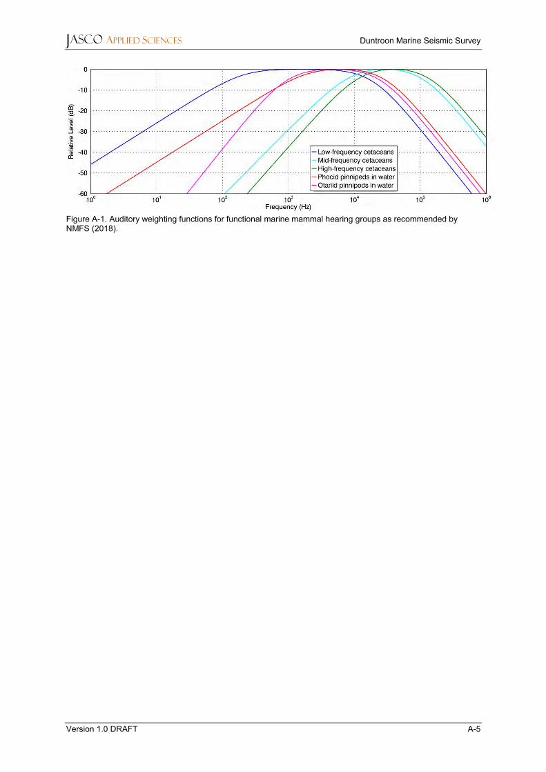
JASCO APPLIED SCIENCES Duntroon Marine Seismic Survey
Version 1.0 DRAFT A-5
Figure A-1. Auditory weighting functions for functional marine mammal hearing groups as recommended by NMFS (2018).

JASCO APPLIED SCIENCES Duntroon Marine Seismic Survey
Version 1.0 DRAFT B-1
Appendix B. Animal Simulation and Acoustic Exposure Model
To assess the risk of impacts from exposure, an estimate of received sound levels for the animals in the area during operations is required. Sound sources move and so do animals. The sound fields may be complex, and the sound received by an animal is a function of where the animal is at any given time. To a reasonable approximation, the location of the sound source(s) is known, and acoustic modelling can be used to predict the 3-D sound field (Figure 2). The location and movement of animals within the sound field, however, is unknown. Realistic animal movement within the sound field can be simulated, and repeated random sampling (Monte Carlo)—achieved by simulating many animals within the operations area—used to estimate the sound exposure history of animals during the operation. Monte Carlo methods provide a heuristic approach for determining the probability distribution function (PDF) of complex situations, such as animals moving in a sound field. The probability of an event’s occurrence is determined by the frequency with which it occurs in the simulation. The greater the number of random samples, in this case the more simulated animals (animats), the better the approximation of the PDF. Animats are randomly placed, or seeded, within the simulation boundary at a specified density (animats/km2). The animat density is much higher than the real-world density to ensure good representation of the PDF. The resulting PDF is scaled using the real-world density.
Several models for marine mammal movement have been developed (Ellison et al. 1987, Frankel et al. 2002, Houser 2006). These models use an underlying Markov chain to transition from one state to another based on probabilities determined from measured swimming behaviour. The parameters may represent simple states, such as the speed or heading of the animal, or complex states, such as likelihood of participating in foraging, play, rest, or travel. Attractions and aversions to variables like anthropogenic sounds and different depth ranges can be included in the models.
Analysis in this report uses the JASCO Animal Simulation Model Including Noise Exposure (JASMINE) 2017. JASMINE uses the same animal movement algorithms as the ‘Marine Mammal Movement and Behavior’ (3MB) model (Houser 2006) but has been extended for use with JASCO-formatted acoustic fields, inclusion of source tracks, and for animats to change behavioural states based on modelled variables such as received level. JASMINE also includes aversion in response to realistic received levels.
B.1. Animal Movement Parameters
JASMINE uses previously measured behaviour to forecast behaviour in new situations and locations. The parameters used for forecasting realistic behaviour are determined (and interpreted) from marine species studies (e.g., tagging studies). Each parameter in the model is described as a probability distribution. When limited or no information is available for a species parameter, a Gaussian or uniform distribution may be chosen for that parameter. For the Gaussian distribution, the user determines the mean and standard deviation of the distribution from which parameter values are drawn. For the uniform distribution, the user determines the maximum and minimum distribution from which parameter values are drawn. When detailed information about the movement and behaviour of a species are available, a user-created distribution vector, including cumulative transition probabilities, may be used (referred to here as a vector model; Houser 2006). Different sets of parameters can be defined for different behaviour states. The probability of an animat starting out in or transitioning into a given behavioural state can in turn be defined in terms of the animat’s current behavioural state, depth, and the time of day. In addition, each travel parameter and behavioural state has a termination function that governs how long the parameter value or overall behavioural state persists in simulation.
The parameters used in JASMINE describe animal movement in both the vertical and horizontal planes. The parameters relating to travel in these two planes are briefly described below.

JASCO APPLIED SCIENCES Duntroon Marine Seismic Survey
Version 1.0 DRAFT B-2
B.1.1.1. Travel sub-models Direction–determines the animat’s choice of direction in the horizontal plane. Sub-models are available for determining the bearing of animats, allowing for movement to range from strongly biased to undirected. A random walk model can be used for behaviours with no directional preference, such as feeding and playing. In a random walk, all bearings are equally likely at each parameter transition time step. A correlated random walk can be used to smooth the changes in bearing by using the current bearing as the mean of the distribution from which to draw the next heading. An additional variant of the correlated random walk is available that includes a directional bias for use in situations where animals have a preferred absolute direction, such as migration. A user-defined vector of directional probabilities can also be defined to control animat bearing. For more detailed discussion of these parameters, see (Houser 2006) and (Houser and Cross 1999).
Travel rate–defines the rate of travel of an animat in the horizontal plane. When combined with vertical speed and dive depth, the dive profile of the animat is produced.
B.1.1.2. Dive sub-models Ascent Rate–defines the rate of travel of an animat in the vertical plane during the ascent portion of a dive.
Descent Rate–defines the rate of travel of an animat in the vertical plane during the descent portion of a dive.
Depth–defines the maximum depth to which an animat will dive.
Bottom Following–determines whether an animat returns to the surface once reaching the ocean floor, or whether it follows the contours of the bathymetry.
Reversals–determines whether multiple vertical excursions occur once reaching the maximum dive depth. This behaviour is used to emulate the foraging behaviour of some marine mammal species at depth. Reversal-specific ascent and descent rates may be specified.
Surface Interval–determines the amount of time spent at the surface prior to performing another dive.

JASCO APPLIED SCIENCES Duntroon Marine Seismic Survey
Version 1.0 DRAFT C-1
Appendix C. Animat Behavioural Parameters
C.1. Nearshore SRW
Table C-1. Animat behavioural parameters for nearshore SRW (females and calves) (number values represent Means (SD) unless otherwise indicated). The parameters are derived from published data on SRW migratory and swim/dive behaviour (Mate et al. 2011, Hain et al. 2013, Mackay et al. 2015) and complemented by data published on northern right whales (Winn et al. 1986, Baumgartner and Mate 2003, Baumgartner and Mate 2005, Mellinger et al. 2007, Kenney 2009).
Behavior Variable Value
Foraging
Travel Direction Correlated Random Walk
Perturbation value 10
Termination coefficient 0.2
Travel rate (m/s) Gaussian 0.44 (0.16)
Ascent rate (m/s) Gaussian 1.47 (0.26)
Descent rate (m/s) Gaussian 1.4 (0.3)
Average depth (m) Gaussian 8.0 (5.0)
Bottom following No
Reversals Gaussian 0.7 (0.2)
Probability of reversal 0.7
Reversal Ascent Dive Rate (m/s) 0.01 (0.01)
Reversal Descent Dive Rate (m/s) 0.01 (0.01)
Time in Reversal (s) Gaussian 420 (60)
Surface interval (s) Gaussian 187.8 (59.4)
Bout duration (s) Gaussian 3600 (600)
V-shaped
Travel Direction Correlated Random Walk
Perturbation value 10
Termination coefficient 0.2
Travel rate (m/s) Gaussian 0.44 (0.16)
Ascent rate (m/s) Gaussian 1.47 (0.26)
Descent rate (m/s) Gaussian 1.4 (0.3)
Average depth (m) Gaussian 8.0 (5.0)
Bottom following No
Reversals No
Surface interval (s) Gaussian 440 (120)
Bout duration (s) Gaussian 1800 (600)
Other
Travel Direction Correlated Random Walk
Perturbation value 10
Termination coefficient 0.2
Travel rate (m/s) Gaussian 0.44 (0.16)
Ascent rate (m/s) Gaussian 1.47 (0.26)
Descent rate (m/s) Gaussian 1.4 (0.3)
Average depth (m) Gaussian 8.0 (5.0)
Bottom following No

JASCO APPLIED SCIENCES Duntroon Marine Seismic Survey
Version 1.0 DRAFT C-2
Behavior Variable Value
Reversals Random 1.0-10.0
Probability of reversal 0.3
Reversal Ascent Dive Rate (m/s) 0.08 (0.05)
Reversal Descent Dive Rate (m/s) 0.01 (0.01)
Time in Reversal (s) Gaussian 200 (60)
Surface interval (s) Gaussian 440 (120)
Bout duration (s) Gaussian 1200 (600)
General Shore following (m) 5
Depth limit on seeding (m) 5 (minimum), 20 (maximum)

JASCO APPLIED SCIENCES Duntroon Marine Seismic Survey
Version 1.0 DRAFT C-3
C.2. Offshore SRW
Table C-2. Animat behavioural parameters for offshore SRW (juveniles and males) (number values represent Means (SD) unless otherwise indicated). Behavioural parameters are derived from published data on SRW migratory and swim/dive behaviour (Mate et al. 2011, Hain et al. 2013, Mackay et al. 2015) and complemented by data published on northern right whales (Winn et al. 1986, Baumgartner and Mate 2003, Baumgartner and Mate 2005, Mellinger et al. 2007, Kenney 2009).
Behaviour Variable Value
Foraging
Travel Direction Correlated Random Walk
Perturbation value 10
Termination coefficient 0.2
Travel rate (m/s) Gaussian 0.92 (0.1)
Ascent rate (m/s) Gaussian 1.47 (0.26)
Descent rate (m/s) Gaussian 1.4 (0.3)
Average depth (m) Gaussian 121.2 (24.2)
Bottom following No
Reversals Gaussian 1.0 (0)
Probability of reversal 1.0
Reversal Ascent Dive Rate (m/s) 0.01 (0.01)
Reversal Descent Dive Rate (m/s) 0.01 (0.01)
Time in Reversal (s) Gaussian 420 (60)
Surface interval (s) Gaussian 187.8 (59.4)
Bout duration (s) Gaussian 3600 (600)
V-shaped
Travel Direction Correlated Random Walk
Perturbation value 10
Termination coefficient 0.2
Travel rate (m/s) Gaussian 0.92 (0.1)
Ascent rate (m/s) Gaussian 1.47 (0.26)
Descent rate (m/s) Gaussian 1.4 (0.3)
Average depth (m) Gaussian 121.2 (24.2)
Bottom following No
Reversals No
Surface interval (s) Gaussian 440 (120)
Bout duration (s) Gaussian 1800 (600)
Other
Travel Direction Correlated Random Walk
Perturbation value 10
Termination coefficient 0.2
Travel rate (m/s) Gaussian 0.92 (0.1)
Ascent rate (m/s) Gaussian 1.47 (0.26)
Descent rate (m/s) Gaussian 1.4 (0.3)
Average depth (m) Gaussian 121.2 (24.2)
Bottom following No
Reversals Random 1.0-10.0
Probability of reversal 0.3
Reversal Ascent Dive Rate (m/s) 0.08 (0.05)

JASCO APPLIED SCIENCES Duntroon Marine Seismic Survey
Version 1.0 DRAFT C-4
Behaviour Variable Value
Reversal Descent Dive Rate (m/s) 0.01 (0.01)
Time in Reversal (s) Gaussian 200 (60)
Surface interval (s) Gaussian 440 (120)
Bout duration (s) Gaussian 1200 (600)
General Shore following (m) 5
Depth limit on seeding (m) 5 (minimum), 20 (maximum)

JASCO APPLIED SCIENCES Duntroon Marine Seismic Survey
Version 1.0 DRAFT D-1
Appendix D. Modelled Animal Exposures
The numbers of modelled animats exposed to acoustic levels exceeding different behaviour thresholds are presented in Table D-1. These results are based upon 0.5 animats/km2.
Table D-1. Counts of modelled animats exposed to acoustic levels exceeding thresholds specified by (Wood et al. 2012, [NMFS] National Marine Fisheries Service 2013).
Sub-population Counts of modelled animats exposed to specific sound levels
120 dB (LP,LF) 140 dB (LP,LF) 160 dB (LP,LF) 160 dB (LP)
Offshore SRW 21402 4573 1366 2078
Nearshore SRW 12480 0 0 0
Lp,LF – denotes low-frequency weighted sound pressure level and has a reference value of 1 µPa Lp - denotes sound pressure level and has a reference value of 1 µPa LE - denotes cumulative sound exposure over a 24-hour period and has a reference value of 1 µPa2s
The exposures as a proportion of the modelled sub-populations of 211,781 (offshore SRW) and 148,650 animats (nearshore SRW), are given in Table D-2.
Table D-2. Modelled animats that were exposed to sound pressure levels exceeding behavioural thresholds as a percentage of the number of animats modelled.
Sub-population Counts of modelled animats exposed to specific sound levels
120 dB (LP,LF) 140 dB (LP,LF) 160 dB (LP,LF) 160 dB (LP)
Offshore SRW 13.79% 2.95% 0.88% 1.34%
Nearshore SRW 5.89% 0.00% 0.00% 0.00%
Lp,LF – denotes low-frequency weighted sound pressure level and has a reference value of 1 µPa Lp - denotes sound pressure level and has a reference value of 1 µPa
In the nearshore behavioural simulations, no animats were exposed to levels exceeding the threshold for injurious effects (PTS). The following discussion should be considered in terms of the seeding density of the animats, which was 0.5 animats/km2,which is greater than the real-world density of SRW. For the offshore sub-population, the simulation predicts that 21 animats, representing 0.01% of the modelled population, would be exposed to a weighted, SEL24h greater than 183 dB and thus experience PTS when applying the NMFS (2018) criteria. All animats which received this sound level were within 500 m of the airgun source, which is less than the predicted maximum distance for the PTS isopleth in the modelling study, which was 760 m. The simulation resulted in 1636 animats (1.03%) exposed to a weighted, SEL24h greater than 168 dB 1 µPa2s, and thus experience TTS when applying the NMFS (2018) criteria. For both PTS and TTS, the few animats (5 and 21) that were exposed to peak pressure levels (PK) exceeding thresholds were also exposed to levels above the SEL24h threshold. However, it is important to note that the model does not account for shutdowns, and all animats which received PTS are within the 2 km low-power and 500 m shutdown range required by the Australian Environment Protection and Biodiversity Conservation (EPBC) Act Policy Statement 2.1, Department of the Environment, Water, Heritage and the Arts (DEWHA) (2008).

JASCO APPLIED SCIENCES Duntroon Marine Seismic Survey
Version 1.0 DRAFT D-2
Table 7. Population-scaling of animat modelling results for entire SRW population (uncorrected for spatial correlation). Scaling number of animat exposed to sound pressure levels exceeding the noise exposure criteria based on number of SRW for entire Australian population.
Sub-population Correction factor [%]
120 dB (Lp,LF)
140 dB (Lp,LF)
160 dB (Lp,LF)
160 dB (Lp)
TTS†
168 dB
(LE, LF)
PTS†
183 dB
(LE, 24h)
Offshore SRW (males/juveniles)
0.19 40.90 8.74 2.61 3.97 3.13 0.04
Nearshore SRW (females/calves)
0.31 39.06 0 0 0 0 0
Lp,LF – denotes low-frequency weighted sound pressure level and has a reference value of 1 µPa Lp - denotes sound pressure level and has a reference value of 1 µPa LE - denotes cumulative sound exposure over a 24-hour period and has a reference value of 1 µPa2s †The model does not account for shutdowns.
Table 8. Population-scaling of animat modelling results for eastern SRW population (uncorrected for spatial correlation). Scaling number of animat exposed to sound pressure levels exceeding the noise exposure criteria based on number of SRW for eastern Australian population.
Correction factor [%]
120 dB(LP,LF) 140 dB(LP,LF) 160 dB(LP,LF) 160 dB(LP)
TTS†
168 dB
(LE, LF)
PTS†
183
(LE, LF, 24h)
Offshore SRW (males/juveniles)
0.02 4.32 0.92 0.28 0.42 0.33 0
Nearshore SRW (females/calves)
0.03 4.13 0 0 0 0 0
Lp,LF – denotes low-frequency weighted sound pressure level and has a reference value of 1 µPa Lp - denotes sound pressure level and has a reference value of 1 µPa LE - denotes cumulative sound exposure over a 24-hour period and has a reference value of 1 µPa2s †The model does not account for shutdowns.