Drillpipe Rotation Effects on Pressure Losses
87
Drillpipe Rotation Effects on Pressure Losses Thorbjørn Lejon Skjold Earth Sciences and Petroleum Engineering Supervisor: Pål Skalle, IPT Department of Petroleum Engineering and Applied Geophysics Submission date: June 2012 Norwegian University of Science and Technology
-
Upload
independent -
Category
Documents
-
view
5 -
download
0
Transcript of Drillpipe Rotation Effects on Pressure Losses

Drillpipe Rotation Effects on Pressure Losses
Thorbjørn Lejon Skjold
Earth Sciences and Petroleum Engineering
Supervisor: Pål Skalle, IPT
Department of Petroleum Engineering and Applied Geophysics
Submission date: June 2012
Norwegian University of Science and Technology


1
Abstract Keeping control of the downhole pressure is important in any drilling situation, and especially
when a narrow pressure window is experienced. The equivalent circulation density is
influenced by rotation of the drillpipe, but there is no existing mathematical description for
this behavior.
In present project, existing knowledge of how drillpipe rotation affects pressure losses was
presented, and used as a foundation in the development of empirical equations through
regression analysis. Several data sets were gathered from various field studies, and a set of
working equations was developed. The equations were presented in two different forms. One
equation expressed pressure losses with rotation and without rotation, ΔPω≠0/ΔPω=0 vs.
revolutions per minute. The three other equations describes ΔPω≠0/ΔPω=0 vs. Reynolds
number, for selected rotation speeds.
The four equations were tested for their accuracy by comparing with simulations performed in
the software Drillbench®, by comparing with an existing mathematical model, and by
comparing with virgin field data. All equations gave predictions close to the existing semi-
empirical model. The equation described as a function of RPM predicted a smaller pressure
loss ratio than the field study for a rotation speed of 60 RPM, but came within the results from
this study for a rotation speed of 120 RPM. The equations expressed as a function of
Reynolds number gave results closer to the semi-empirical model than the RPM-equation. All
equations predicted a larger pressure loss than the simulations performed in Drillbench®, in
some cases even twice as large.
To further improve the equations, larger data sets have to be acquired. The quality of the
equations will improve if they cover more situations, and if they are based on a wider spread
in the data sets.

2
Sammendrag Å holde kontroll på nedi hulls trykk er viktig i alle boresammenhenger, og spesielt når et
trangt trykkvindu oppleves. ECD blir påvirket av rotasjon av borestrengen, men det eksisterer
ingen matematisk formel som beskriver dette bidraget.
I dette prosjektet ble den eksisterende kunnskap om hvordan rotasjon av borestrengen
påvirker trykktap i ringrom presentert og brukt som et grunnlag under utviklingen av
empiriske formler gjennom regresjonsanalyse. Datasett ble samlet inn fra flere feltstudier, og
et sett av funksjonelle ligninger ble utviklet. Ligningene ble presentert på to ulike former. En
ligning uttrykker trykktap med rotasjon og uten rotasjon, ΔPω≠0/ΔPω=0 mot rotasjoner per
minutt. De tre andre ligningene beskriver ΔPω≠0/ΔPω=0 mot Reynolds tall, for utvalgte
rotasjonshastigheter.
De fire ligningene ble testet for deres nøyaktighet ved å sammenligne med simuleringer i
programvaren Drillbench®, ved å sammenligne med en eksisterende matematisk modell, og
ved å sammenligne med ubrukt feltdata. Alle ligningene gav resultater nær den eksiterende
delvis empiriske modellen. Ligningen som ble beskrevet som en funksjon av
rotasjonshastighet anslo lavere rater for trykktap enn feltstudiet for en rotasjonshastighet på
60 rotasjoner per minutt, men kom innenfor intervallet i studiet ved en rotasjonshastighet på
120 rotasjoner i minuttet. Ligningene uttrykt som en funksjon av Reynolds tall gav resultater
nærmere den delvis empiriske modellen enn ligningen for rotasjonshastighet. Alle ligningene
gav et høyere trykktap enn resultatene fra Drillbench®-simuleringene, i noen tilfeller dobbelt
så stort.
For å videreutvikle ligningene er det et behov for større datasett. Kvaliteten på ligningene vil
bli bedre dersom de dekker flere situasjoner, og dersom de er utviklet fra datasett med en
større spredning.

3
Table of Contents Abstract .................................................................................................................................................. 1
Sammendrag .......................................................................................................................................... 2
Chapter 1: Introduction ........................................................................................................................ 9
Chapter 2: Previous Published Work on Rotational Effects on ECD ............................................ 11
2.1: ECD Control: Influence of Annulus Pressure Drops in General ................................................ 11
2.1.1: Annular Friction .................................................................................................................. 12
2.1.2: Cuttings Effect ..................................................................................................................... 12
2.1.3: Surge and Swab ................................................................................................................... 13
2.1.4: Gelling ................................................................................................................................. 14
2.1.5: Acceleration ........................................................................................................................ 14
2.2: Rotation of Drillstring ................................................................................................................ 14
2.3: Knowledge from Previous Studies on Rotational Effects .......................................................... 16
2.3.1: Field Testing vs. Theoretical Approach .............................................................................. 16
2.3.2: Experimental Results ........................................................................................................... 18
Chapter 3: The PLR-Equation ........................................................................................................... 21
Chapter 4: The Drillbench® Software: for Comparison Purposes ................................................. 23
4.1: Presentation of Software ............................................................................................................ 23
4.2: Simulation Base Case Data Set .................................................................................................. 24
4.2.1: Formation Parameters ......................................................................................................... 25
4.2.2: Survey Parameters ............................................................................................................... 25
4.2.3: Pore Pressure and Fracture Pressure Parameters ................................................................. 27
4.2.4: Wellbore Geometry Parameters .......................................................................................... 27
4.2.5: String Input Parameters ....................................................................................................... 27
4.2.6: Mud Input Parameters ......................................................................................................... 28
4.2.7: Temperature Input Parameters ............................................................................................ 29
4.3: Results of Drillbench® Simulations ............................................................................................ 29
Chapter 5: Development of Own Models Through Regression Analysis ....................................... 33
5.1: Data Sets Generation .................................................................................................................. 33
5.2: Resulting Regressed Equations .................................................................................................. 41
5.3: Results ........................................................................................................................................ 44
5.3.1: Comparison With Drillbench® Simulations .......................................................................... 44
5.3.2: Comparison With PLR-Equation and a Field Study.............................................................. 47

4
Chapter 6: Discussion and Evaluation of Work ............................................................................... 49
6.1 Data Quality ................................................................................................................................ 49
6.2 Model Quality ............................................................................................................................. 49
6.3 Future Improvements .................................................................................................................. 50
Chapter 7: Conclusion ........................................................................................................................ 53
References ............................................................................................................................................ 55
Abbreviations ....................................................................................................................................... 57
Nomenclature ....................................................................................................................................... 59
N.1 Roman ................................................................................................................................... 59
N.2 Greek ..................................................................................................................................... 59
Appendix A: Well Data from SPE 24596 ............................................................................................. i
Appendix B: Well Data from SPE 59265 ............................................................................................ v
Appendix C: Well Data from SPE 87149 .......................................................................................... vii
Appendix D: Well Data from SPE 19526 ......................................................................................... xiii
Appendix E: Well Data from SPE 110470 ........................................................................................ xv
Appendix F: Well Data from SPE 26343 ......................................................................................... xvii
Appendix G: Input Values for Calculations with PLR-Equation .................................................. xix
Appendix H: Calculation Inputs ..................................................................................................... xxiii
Unit Conversion Factors ................................................................................................................... xxv
List of Figures Fig. 1—ESD and rotational effects plotted into pressure window (Skjold 2011) .................................. 11
Fig. 2—ECD and rotational effects plotted into pressure window (Skjold 2011).................................. 12
Fig. 3—Fluid movement when tripping out of hole (free after Skalle, 2010) ....................................... 13
Fig. 4—Laminar fluid flow in the annulus .............................................................................................. 15
Fig. 5—Formation of Taylor vortices when pipe is rotated resulting in ”turbulent-like” mixing .......... 15
Fig. 6—Drillbench® input parameters for formation ............................................................................. 25
Fig. 7—Drillbench® input parameters for survey .................................................................................. 26
Fig. 8—Drillbench® input parameters for wellbore geometry .............................................................. 27
Fig. 9—Drillbench® input parameters for string components .............................................................. 27
Fig. 10—Drillbench® input parameters for mud properties ................................................................. 28
Fig. 11—Fann readings used as rheology model input with fluid density of 1300 kg/m3 ..................... 29
Fig. 12—Fann reading used as rheology model input with fluid density of 1500 kg/m3 ...................... 29

5
Fig. 13—Fann reading used as rheology model input with fluid density of 1700 kg/m3 ...................... 29
Fig. 14—Resulting plot of ECD versus time for 1300 kg/m3 drilling fluid .............................................. 30
Fig. 15—Resulting plot of ECD versus time for 1500 kg/m3 drilling fluid .............................................. 30
Fig. 16—Resulting plot of ECD versus time for 1700 kg/m3 drilling fluid .............................................. 31
Fig. 17—Plot of gathered data on the form ΔPω≠0/ΔPω=0 vs. RPM ......................................................... 42
Fig. 18—Plot of gathered data on the form ΔPω≠0/ΔPω=0 vs. Re for 200 RPM rotation speed .............. 42
Fig. 19—Plot of gathered data on the form ΔPω≠0/ΔPω=0 vs. Re for 300 RPM rotation speed .............. 43
Fig. 20—Plot of gathered data on the form ΔPω≠0/ΔPω=0 vs. Re for 600 RPM rotation speed .............. 43
Fig. 21—Well 578P1172 characteristics ................................................................................................... i
Fig. 22—Effect of rod rotation speeds on annular pressure losses for well 578P1172 ........................... i
Fig. 23—Total pressure losses in function of mud flow rates and rotation speed for well 578P1172 ....ii
Fig. 24—Well 425P1210 characteristics ...................................................................................................ii
Fig. 25—Effect of rod rotation speeds on annular pressure losses for well 425P1210 ...........................ii
Fig. 26—Total pressure losses in function of mud flow rates and rotation speed for well 425P1210 ... iii
Fig. 27—Well 425P2078 characteristics .................................................................................................. iii
Fig. 28—Effect of rod rotation speeds on annular pressure losses for well 425P2078 .......................... iii
Fig. 29—Total pressure losses in function of mud flow rates and rotation speed for well 425P2078 ... iv
Fig. 30—Effects of drillpipe rotation speed on annular pressure losses in the Miao 1-40 well .............. v
Fig. 31—Fluid and cuttings properties with water as drilling fluid ........................................................ vii
Fig. 32—Fluid properties for Mud A and Mud B drilling fluids .............................................................. vii
Fig. 33—Bottomhole pressure versus rotary speed. Drilling fluid is water, Q=0.022 m3/s .................. viii
Fig. 34—Bottomhole pressure versus rotary speed. Drilling fluid is water, Q=0.028 m3/s .................. viii
Fig. 35—Bottomhole pressure versus rotary speed. Drilling fluid is water, Q=0.035 m3/s .................... ix
Fig. 36—Bottomhole pressure versus rotary speed. Drilling fluid is Mud A, Q=0.022 m3/s ................... ix
Fig. 37—Bottomhole pressure versus rotary speed. Drilling fluid is Mud A, Q=0.028 m3/s .................... x
Fig. 38—Bottomhole pressure versus rotary speed. Drilling fluid is Mud A, Q=0.035 m3/s .................... x
Fig. 39—Bottomhole pressure versus rotary speed. Drilling fluid is Mud B, Q=0.022 m3/s ................... xi
Fig. 40—Bottomhole pressure versus rotary speed. Drilling fluid is Mud B, Q=0.028 m3/s ................... xi
Fig. 41—Bottomhole pressure versus rotary speed. Drilling fluid is Mud B, Q=0.035 m3/s .................. xii
Fig. 42—ΔPω≠0/ΔPω=0 plotted against the Reynolds number for three rotation speeds ....................... xiii
Fig. 43—Measured Change in ECD plotted against RPM for Elf 8.75-in A and Elf 8.75-in B .................. xv
Fig. 44—Annular pressure plotted against flow rate. RPM is 300 and 600 ......................................... xvii
Fig. 45—Log-log plot from Herschel-Bulkley 3 point oil field approach by use of 1300 kg/m3 mud .... xix

6
Fig. 46—Log-log plot from Herschel-Bulkley 3 point oil field approach by use of 1500 kg/m3 mud ..... xx
Fig. 47—Log-log plot from Herschel-Bulkley 3 point oil field approach by use of 1700 kg/m3 mud .... xxi
List of Tables Table 1—Pressure losses vs. RPM data from 578P1172 well ............................................................... 34
Table 2—Pressure losses vs. RPM data from 425P1210 well ............................................................... 34
Table 3—Pressure losses vs. RPM data from well 425P2078 well ........................................................ 35
Table 4—Pressure losses vs. RPM from Miao 1-40 well ....................................................................... 35
Table 5—Data of pressure losses vs. RPM collected from BETA well. Water as the drilling fluid ........ 36
Table 6—Data of pressure losses versus RPM collected from BETA well. Mud A as the drilling fluid.. 36
Table 7—Data of pressure losses versus RPM collected from BETA well. Mud B as the drilling fluid .. 37
Table 8—Welldata from the 22/30c-G4 well ........................................................................................ 37
Table 9—Welldata from 578P1172 on the form ΔPω≠0/ΔPω=0 vs. Reynolds number, RPM=200 ........... 38
Table 10—Welldata from 425P1210 on the form ΔPω≠0/ΔPω=0 vs. Reynolds number, RPM=200 ......... 38
Table 11—Welldata from SHADS #7 on the form ΔPω≠0/ΔPω=0 vs. Reynolds number, RPM=200 .......... 39
Table 12—Welldata from 425P2078 on the form ΔPω≠0/ΔPω=0 vs. Reynolds number, RPM=300 ......... 39
Table 13—Welldata from SHDT.1 on the form ΔPω≠0/ΔPω=0 vs. Reynolds number, RPM=300 .............. 40
Table 14—Welldata from SHDT.1 on the form ΔPω≠0/ΔPω=0 vs. Reynolds number, RPM=600 ............. 40
Table 15—Welldata from SHADS #7 on the form ΔPω≠0/ΔPω=0 vs. Reynolds number, RPM=600 .......... 41
Table 16—Comparison of results from simulation and ΔPω≠0/ΔPω=0 vs. RPM–eq., MW=1300 kg/m3 .. 45
Table 17—Comparison of results from simulation and ΔPω≠0/ΔPω=0 vs. RPM–eq., MW=1500 kg/m3 .. 45
Table 18—Comparison of results from simulation and ΔPω≠0/ΔPω=0 vs. RPM–eq., MW=1700 kg/m3 .. 45
Table 19—Drillbench® simulation compared with ΔPω≠0/ΔPω=0 vs. Re–equations for laminar flow ..... 46
Table 20—Drillbench® simulation compared with ΔPω≠0/ΔPω=0 vs. Re–equations for turbulent flow .. 46
Table 21—ΔPω≠0/ΔPω=0 vs. RPM–equation compared to PLR–equation and field study. ...................... 47
Table 22—Comparison of PLR–equation and ΔPω≠0/ΔPω=0 vs. Re-equations for laminar flow. ............ 48
Table 23—Comparison of PLR–equation and ΔPω≠0/ΔPω=0 vs. Re-equations for turbulent flow. ......... 48
Table 24—Input values in PLR–calculations. MW is 1300 kg/m3 .......................................................... xix
Table 25—Input values in PLR-calculations. MW is 1500 kg/m3 ............................................................ xx
Table 26—Input values in PLR-calculations. MW is 1700 kg/m3 ........................................................... xxi
Table 27—Input values for 578P1172 calculations ............................................................................. xxiii
Table 28—Input values for 425P1210 calculations ............................................................................. xxiii
Table 29—Input values for 425P2078 calculations ............................................................................. xxiii

7
Table 30—Input values for SHDT.1 calculations ................................................................................. xxiv
Table 31—Conversion factors from oil field units to SI units ............................................................... xxv
Table 32—Conversion factors from other units SI units ...................................................................... xxv

8

9
Chapter 1: Introduction Handling of the downhole pressure and its variation is important for various reasons. Both the
cleaning aspect and the pressure limitations are of great importance. The added contribution
of drillstring rotation on the equivalent circulation density (ECD) can in some situations be of
such a magnitude that impossible drilling conditions are experienced. In situations with
narrow pressure window, accurate prediction of ECD is crucial, though there is no existing
common equation representing the rotational contribution. Up to now, the problem has been
solved with a variety of equations developed from specific field experiments, or semi-
theoretical equations, but with strong limitations on their usability.
In this thesis, empirical equations of how drillstring rotation is affecting ECD in general will
be derived through regression analysis of collected drilling data. The accuracy of these
equations will be tested through example calculations by use of a new set of drilling data. In
addition, the empirical equations will be compared to an existing semi-empirical equation
expressing drillpipe rotation effects and simulations of ECD from the software Drillbench®.
This software is chosen on basis of its availability and reputation in the industry. Allthough
the software do not reveal its model of rotational effects, it can be helpful in testing the
accuracy of the empirical equations developed through present project. The goal of this
project is to develop empirical equations for the rotational contribution of ECD and make
them applicable to all possible scenarios, with as few simplifications as possible, and without
compromising with the limitations of the equation.
To reach this goal, a stepwise approach is needed. The first step will be to acquire enough
knowledge on the problematical areas within drillstring rotation, discuss and evaluate the
problems, and find possible solutions on how to express them mathematically. Here we will
present why field data show increased pressure loss in the laminar area while theoretical
evaluation leads to reduced pressure loss. Step two will be to gather a largest possible data
bank of pressure vs. rotation during pumping. Step three will consist of data arranging and
regression analysis to obtain a set of working equations. The last step will be to test the
accuracy and usability of the models, by comparing the equations to real drilling data, the
semi-empirical equation, and to the Drillbench® simulations.

10

11
Chapter 2: Previous Published Work on Rotational Effects on ECD This chapter will provide a theoretical foundation for the understanding of drillstring
rotational effects on ECD. It is roughly divided into two parts; the first part will provide
information of the most important topics that might interfere with drillstring rotational effects
and ECD, along with a presentation of pipe rotation in laminar and turbulent fluid flows. The
second part will be a presentation of previous published work on drillstring rotation.
2.1: ECD Control: Influence of Annulus Pressure Drops in General
Equivalent circulation density can be understood as the total actual bottomhole pressure
exerted on the formation (Skalle 2010), and is the sum of equivalent static density (ESD) and
the pressure increments experienced from pressure drops along the annulus, and the extra
weight of drill cuttings contained in the annulus. Controlling the ECD is especially important
when drilling long, horizontal well sections, deepwater drilling, drilling through depleted
reservoirs, and for other wellbores where a narrow pressure window is experienced. From
Fig. 1 and Fig. 2 it can be seen why controlling ECD is important. Fig. 1 show the ESD
gradient for a well drilled in a depleted reservoir, along with the ESD gradient plus the
rotational contribution of the ECD, plotted with the pore pressure gradient and fracture
pressure gradient versus depth. Fig. 2 shows the plot of the ECD gradient with rotational
effects. As can be seen from this figure, the additional pressure increment in ECD causes the
bottomhole pressure to exceed the upper pressure limit, leading to impossible drilling
conditions.
Fig. 1—ESD and rotational effects plotted into pressure window (Skjold 2011).

12
Fig. 2—ECD and rotational effects plotted into pressure window (Skjold 2011).
A general equation to express ECD, with the different pressure drops included, is presented
below:
, &friction annular cuttings surge swab rotation accelerationmud
p p p p pECD
gzρ
∆ + ∆ + ∆ + ∆ + ∆= + (2.1)
As can be seen from the equation, the various pressure increments arise from various sources.
Normally the effects of increasing temperature with increasing depth, and increasing
hydrostatic pressure with increasing depth, are ignored when calculating ECD (Skalle 2010).
2.1.1: Annular Friction
Pressure loss resulting from annular friction is caused by the fluid’s motion against an
enclosed surface, such as a pipe (OilGasGlossary 2012). When a fluid is flowing through a
pipe, the friction within the fluid and against the pipe wall creates pressure losses. Annular
friction is most accurately estimated by selecting the best fitting rheological model, whether
this is the Newtonian model, the Bingham model, the Herschel-Buckley model or the Power
law model.
2.1.2: Cuttings Effect
In a horizontal well there is a certain amount of cuttings in suspension, and these cuttings
contribute with a pressure loss increment. Some of the cuttings settle, some are inside the mud
flow, and some are lifted by lifting forces in the mud flow. These cutting amounts affect the
-
500
1 000
1 500
2 000
2 500
0,0 10,0 20,0 30,0 40,0 50,0 60,0
Pressure [MPa]
Dep
th [m
]
Fracture PressurePore PressureECD + Rotation

13
mud weight (MW), and thereby the bottomhole pressure. It is not easy to predict without
assuming some of the values, though a set of equations to estimate the pressure loss do exist:
,cuttings cuttings averagep g TVDρ∆ = ⋅ ⋅ (2.2)
In this equation, ρcuttings,average is expressed by:
, , ,(1 )cuttings average mud cuttings average cuttings cuttings averagec cρ ρ ρ= − + ⋅ (2.3)
Rotation of the drillstring will influence this pressure loss by changing how large the cutting
beds will be (Skalle 2010).
2.1.3: Surge and Swab
Surge and swab is the term used when talking about pressure changes from tripping
operations. When tripping out, the bottomhole pressure will decrease because of friction
between the moving pipe and the stationary drilling fluid. This pressure is referred to as swab
pressure. A bottomhole pressure increase will be seen when tripping into the hole, referred to
as swab pressure (New Mexico Tech 2012). The downward mud movement experienced
when tripping out of hole is shown in Fig. 3. The green line indicates the mud position before
the operation is started, while the red lines indicate how the mud is displacing the void left by
the upward movement of the pipe.
Fig. 3—Fluid movement when tripping out of hole (free after Skalle, 2010).

14
2.1.4: Gelling
Gelling is the term used for the gelled structure most drilling fluids form while being at rest
for a certain amount of time. Before being able to circulate, the gel structure has to be broken,
and an extra pressure has to be applied to break the gel on the pipe surface (Skalle 2010). To
get the extra pressure needed, either the pump is used, or simply the pipe is rotated. The gel
breaking pressure is thought to be small, and hidden in the acceleration pressure.
2.1.5: Acceleration
The acceleration pressure is also caused by pipe movement. It is experienced during some
tripping operations, and when a gas kick reaches the surface (Skalle 2010). Acceleration of
the pipe causes an acceleration pressure in the drill fluid. This phenomenon is calculated with
the following equation:
,
,
pipe effectiveacceleration pipe
ann effective
Ap m a L a
Aρ∆ = ⋅ = ⋅ ⋅ ⋅ (2.4)
2.2: Rotation of Drillstring
Rotation of the drillstring could significantly alter the bottomhole pressure, but a series of
studies on pipe rotation show contradictory results of whether this alteration is positive or
negative, as will be explained in detail later. As presented by Skalle (2010), pipe rotation in a
laminar flow will lead to an additional shear velocity component. Normally drill fluids are
shear thinning, and rotation would give an increase in total shear stress, with a decrease of the
viscosity, leading to a reduction of the pressure drop and the corresponding bottomhole
pressure. When rotating the drillpipe, the effective strain rate is increased, the effective
viscosity decreased, with a reduction of the axial pressure drop as a result. In laminar
developed flows of Newtonian fluids (see Fig. 4), viscosity is independent of shear rate, and
the described effects could not take place. At the slowest rotation rates, when both the
Reynolds number and the Taylor number are beneath their critical values, the laminar fluid
flow could be depicted as a helical type flow.

15
Fig. 4—Laminar fluid flow in the annulus.
For most drilling operations, an increased pressure drop will be experienced. This is thought
to be caused by the development of instabilities (Skalle 2010). According to Marken et al.
(1992), rotation of the drillstring would create centripetal forces ‘throwing’ away fluid close
to the pipe, leaving a ’void’. These ‘voids’ are filled with fluid from the outer part of the
annulus. As a result, secondary flow called Taylor vortices are created, as shown in Fig. 5. As
described by Skalle (2010), rotation and the forming of these vortices would lead to an axial-
radial mixing, and this would have the same effect on momentum transport as turbulent
mixing.
Fig. 5—Formation of Taylor vortices when pipe is rotated resulting in ”turbulent-like” mixing.
Because turbulent flow is shear thickening, this effect will lead to an increased pressure drop,
as field studies in the next subchapters will present. In addition to the formation of Taylor
vortices, Marken et al. (1992) presented some additional suggestions as to what causes the
increased pressure drops. During drilling operations with fluid circulation, effects like
drillstring vibration and motion of the pipe will alter the flow regimes. Lateral and rotational

16
motion, along with axial vibration and motion, tend to disrupt fluid flow patterns, giving
another contribution to the ‘turbulent-like’ flow.
2.3: Knowledge from Previous Studies on Rotational Effects
The following sections will reveal existing work regarding rotational effects on ECD. This is
done to give a larger foundation to understand why this project is carried out, and will also
serve as a reference to the relevance of the project. For this topic, the chapter is divided into
two parts, experimental results, and field testing versus theoretical approach. The reason for
this classification is to highlight the differences within the results obtained from the various
procedures. To clarify how the published studies are classified, an explanation of the terms
will now be given. Field testing contains studies based on field measurements, where an
actual well have been used to provide the most realistic conditions, but with limitations on the
accuracy of measurements and the ability to focus on one single part of the process because of
the influence from other phenomenon. An example of field testing is the work of Charlez et
al. (1998). The theoretical approach contains, as the name imply, studies from a theoretical
point of view. Here the studies are more based on theory, with a biased opinion of the
expected results, both from field measurements and from laboratory experiments. An example
study of this is Ahmed & Miska (2008). For the experimental approach, laboratory
measurements and testing of specific parameters is the criteria. An example of such a study is
Hansen & Sterri (1995).
2.3.1: Field Testing vs. Theoretical Approach
A lot of field testing has been carried out to understand how the ECD react to pipe rotation.
Pressure-While-Drilling (PWD) was used to obtain data in several extended reach wells
(ERD) in the North Sea (Charlez et al. 1998), and this data was used to investigate drillpipe
rotation effects on ECD. From a series of drillstring rotation tests, it was found that for a
constant flow rate, rotation of the drillpipe would increase close to linearly with the rotation
speed. This was found in a 12¼-in. hole with a flow rate of 0.045 m3/s, and in an 8½-in. hole
with constant flow rate of 0.028 m3/s. In the same test, it could be seen that the increase
would be larger in the latter case. Testing was also performed for different flow rates with
several rotation speeds. This test shows that flow rate does not change the trend from the first
test; an increased ECD will be seen with increased drillstring rotation speed.

17
These results were supported by Bertin et al. (1998). Through this work it was also found that
pipe rotation would have a positive effect on ECD, and that it was almost linear with the pipe
revolutions per minute (RPM). The results suggested an ECD increase resulting from pipe
rotation of around 10 kg/m3 for every 60 RPM increase.
A study by Andreassen & Ward (1997) of PWD measurements from Statfjord and Gullfaks
also concluded that rotation of the drillstring would lead to an ECD increase, and especially
for high rotation speed (above 50 RPM). It was found that depending on the drilling fluid
used, rotation could increase the ECD with between 50% and 100% compared to that with no
rotation. Rotation speeds less than 50 RPM was found not to give any important contribution
to ECD, and this was thought to be owing to the uneven mud weights, and that cutting loads
affected the measured data.
Bode et al. (1989) presented a study of slim-hole drilling. Through tests performed in the
well, an increased pressure loss could be seen when the drillstring was rotated. The
bottomhole ECD showed 12.1 lbm/gal with no rotation, while a rotation speed of 600 RPM
increased the ECD value to 16.1 lbm/gal. Another study of slim-hole drilling (Delwiche et al.
1992) also gave an increased pressure loss. In this study, the pressure loss inside annulus
because of drillstring rotation was found to be larger for a slim hole compared to a
conventional hole, but in both situations an increase was seen.
Other studies show similar results, a narrow borehole will give a larger increase in pressure
losses when drillpipe is rotated. McCann et al. (1993) and Haige et al. (2000) conducted
experiments on this topic. These results will be thoroughly presented in the next section, but
both of the studies gave affirmative results. Diaz et al. (2004) carried out a theoretical study,
and compared the expected results with field data. It was found that increasing drillstring
rotation speed would lead to increased pressure losses in the annulus. When the annular
clearance decreases, an effect like eccentricity will play a larger role for rotational-induced
pressure losses than what is the case for a regular wellbore.
A combined theoretical and experimental study was performed by Ahmed & Miska (2008). It
was found that for a highly eccentric pipe, rotation indicated presence of shear thinning and

18
inertial effects, which results in increased pressure losses when the pipe is rotated. The inertial
effects could be generated both from eccentricity and from geometric irregularities, or a
combination of these. The presence of inertial effects could affect the velocity field when the
pipe is rotating.
Ahmed et al. (2010) combined field measurements with the theory of pipe rotation to find a
model that could predict the pressure losses as a function of drillpipe rotation. They
developed a semi-empirical model, and with dimensionless input parameters for all the
theoretical expressions. A full presentation of this study will be given in chapter 3, and this
model will later be used to validate the accuracy of the empirical equations developed in this
project.
2.3.2: Experimental Results
Hansen & Sterri (1995) concluded that rotation would decrease the frictional pressure loss for
a helical flow when Reynolds number is kept smaller than the Taylor number, and the Taylor
number is less than the critical Taylor number. However, if the Reynolds number is less than
the critical Reynolds number and the Taylor number is above the critical Taylor number, or if
both the Reynolds number is greater than the critical Reynolds number and the Taylor number
is greater than the critical Taylor number, there will be an increase in the frictional pressure
loss.
In a study conducted by McCann et al. (1993), a 1.25 inch steel shaft within a clear acrylic
tube of diameter 1.375 to 1.75 inch internal diameter were used for sensitive pressure
measurements of fluid flow in a concentric annuli, and a similar test with a clear acrylic tube
of 1.50 inches internal diameter were used to make similar measurements for a fully eccentric
annuli. During the testing, a maximum rotation speed of 900 RPM and a maximum fluid flow
rate of 0.001 m3/s were used. In this experiment it was found that for a laminar flow,
increased pipe rotation would lead to a decreased pressure loss, while for a turbulent flow
increased pipe rotation would give a increased pressure loss. The results obtained in this study
were compared with typical models used by the industry to predict pressure losses from pipe
rotation, and they found that none of them gave satisfying results. It was also seen that
increasing mud rheology would give an increased pressure loss, while increasing eccentricity
would lead to decreased pressure loss, regardless of the flow regime.

19
Similar results were found in a study performed by Hansen et al. (1999). Here a steel tube
with outer diameter of 4.45 cm was placed inside a transparent Plexiglas tube with inner
diameter of 5.08 cm. The steel tube could be placed according to the desired eccentricity of
the annulus. The maximum flow rate used in the experiment was 0.008 m3/s, and a maximum
pipe rotation of 600 RPM. The experiment was conducted to study the influence of pipe
rotation in narrow annuli for various flow regimes, by use of several fluids, and test the
accuracy of existing models for predicting pressure losses. The fluids used were water,
different solutions of CMC (Carboxyl Methyl Cellulose) in water, and different solutions of
Xanthan in water. Water was found to be a Newtonian fluid, water mixed with CMC was
characterized by a two parameter Power law model, water and Xhantan in a mixture would
represent a Bingham fluid, or it was described by a three-point Herschel-Bulkley model if the
lowest shear rates were neglected.
In the experiments it was found that eccentricity would decrease pressure losses relative to
concentric pipe position regardless of the fluid used. Furthermore, for shear thinning fluids
such as CMC solutions, it was found that the frictional pressure losses would be reduced
when rotating the pipe at low flow rates, while increased pressure losses were seen at higher
flow rates.
Another experimental study was conducted by Haige et al. (2000). The testing were
performed by use of a transparent outer pipe with an internal pipe diameter of 5 in., and two
different diameters on the inner pipe, 3 in. and 3.5 in.. The length of the test apparatus was 6
meters. From the test results it was seen that a slow pipe rotation speed would lead to a small
decrease in annular pressure losses. When rotating at speeds above 70 RPM, a rapid increase
in annular pressure losses was experienced. It was found that increasing eccentricity would
quickly decrease the annular pressure losses. By comparing the results from testing done with
the two different inner pipe diameters, it was found that a decreased annular gap would make
the pressures much more sensitive to pipe rotation speed.

20

21
Chapter 3: The PLR-Equation The need for a mathematical model of pipe rotation effects on ECD has been presented earlier
in this project. An effort to make such a model was done by Ahmed et al. (2010). In this
study, a semi-theoretical model was developed based on field studies. The equation obtained
was presented in dimensionless parameters, with the introduction of a key parameter, the
pressure loss ratio (PLR).
0
( / )( / )
dP dLPLRdP dL
ω
ω=
= (3.1)
As can be seen from this equation, the pressure loss ratio is the pressure loss with pipe
rotation divided by pressure loss without rotation. Through dimensionless analysis, the
solution to this equation was described as:
0.428 0.158 0.054 0.0319 0.042 0.01522
10.36 (13.5 ) Re ( 1)yave effPLR n Ta k
U kτ
ερ
−= × + × × × × × − (3.2)
In this equation, ρ represents the fluid density, τy is the Herschel-Bulkley yield stress, and n is
the fluid behavior index from this rheology model. Furthermore, U is the mean annular
velocity, and k is the diameter ratio between the drillpipe and the borehole wall, Dp/Dh. The
other parameters are described with equations. Ta is the Taylor number, described by:
23( )16
p h p
app
D D DTa ρω
µ −
=
(3.3)
In this equation, Dp is the pipe diameter, Dh is the hole diameter, ρ is the fluid density, ω is the
angular speed, and μapp the apparent viscosity.
The parameter εave is the average dimensionless eccentricity, described by:
1
2( )
ni i
avei h p
E LD D MD
ε=
=−∑ (3.4)
Again, Dh and Dp represents the hole diameter and the pipe diameter respectively. MD is the
measured depth, Li is the length of a wellbore section, and Ei is the effective eccentricity
described by:
h TJ
h p
D DED D
−=
− (3.5)
DTJ is here the tool joint diameter, and the other parameters are as previously described. E is
to be calculated for every wellbore section Li.

22
The final parameter to be discribed, is Reeff. This parameter is found with Eq. 3.6:
2
,
8Reeffw lam
Uρτ
= (3.6)
This is how the effective Reynolds number is described. U is the mean annular velocity, and ρ
is the fluid density. The final parameter to be described is τw,lam, which is the average wall
shear stress for a concentric annulus.
The model presented above was derived by analyzing data from field studies, but some of the
studies were omitted because of lacking key parameters required for testing purposes, or data
points were withdrawn because of bad correlation. This was done where it was thought that
inaccuracies from measurements were causing poor correlation to the other data sets. During
model validation, predicted values were compared to measured values from several field
studies, and even though the field studies were taken under various drilling conditions, the
predictions were fairly accurate, with an error of approximately ±15%.
In the development of the empirical equations later in this project, this theoretical model will
be used for comparison purposes, along with the results obtained from the Drillbench®
simulations in the next chapter.

23
Chapter 4: The Drillbench® Software: for Comparison Purposes This chapter will serve as a presentation of the simulation software used in this project. It
consists of two parts, a general description of the software and its possibilities, and a
presentation of simulations done based on a field study.
4.1: Presentation of Software
As previously mentioned, the equations developed in this project will be compared to
simulations performed in software called Drillbench®. This is a commercial software package
owned by the SPT Group. The software suite is used for designing and evaluation of drilling
operations. It consists of three modules, Dynamic Hydraulics, Dynamic Well Control and
Underbalanced Operations. Each of these modules consists of one or more applications. The
Underbalanced Operations-module have two applications, Dynaflodrill and Steadyflodrill,
Dynamic Well Control have one application, called Kick, while Dynamic Hydraulics consist
of three applications, Presmod, Hydraulics and Frictionmaster. Each of these applications is
made to perform specific tasks to one or several parts of the drilling operation.
In this project, the Presmod application is the one used for the simulations. Before the specific
abilities of this application are described, an explanation as to why this software was chosen is
advantageous as a justification to our choice. The Drillbench® software have a good
reputation in the industry. It is used by several major companies, with satisfying results. The
following quotes are feedback of customer experience, taken from SPT Group (2012).
“We have been using Drillbench® Presmod and Kick successfully for well planning and
follow-up. In addition, it has been used for crew training purposes on HPHT wells in the
UK sector.” BP, Aberdeen
“The Drillbench® Presmod dynamic hydraulics simulation program was successfully used
on the Marlin A-5 well: The program produced accurate downhole temperature and
density profiles. The accuracy of the predictions was confirmed by downhole PWD
measurements.” Baker Hughes Inteq, USA
“Both Drillbench® Presmod and Kick have been very useful for decision making in two
difficult HPHT wells and have contributed to us reaching the planned targets.”
ConocoPhilips, Scandinavian Division

24
As can be seen, the software has been used in a variety of situations, and by several major
companies. Many companies use the software on an everyday basis. The software is
continuously improved, and was developed based on more than 15 years of drilling research.
The Drillbench® software was chosen based on its spread in the industry, its reputation, and
the availability for usage in this project. It provides the features desired for comparisons
purposes, and the visualization options give the required possibilities.
Drillbench® presmod is as mentioned the chosen application. In this part of the software, it is
possible to accurately model pressures (ECD and ESD) and temperature profiles for
deepwater wells, high pressure high temperature (HPHT) wells, or other wells with narrow
margins between pore and fracture pressure, such as ERD wells and wells in depleted
reservoirs. This application make it possible to build an imaginary well based on real input
parameters, and by selecting the wanted input parameters according to the well to be modeled,
simulations of various drilling operations can be carried out.
It is possible to select which fluid systems should be used, the maximum and minimum
circulation rates can be chosen, maximum tripping velocities can be set, and from this several
operational procedures within pressure limitations can be developed. For this project, the
possibility of selecting drillpipe rotation speeds, fluid circulation rates, rheology models and
the eccentricity of the pipe, along with the batch simulation feature – choosing which
operation should be performed, and for how long–make the Presmod application suitable for
comparison purposes.
Several simulations can be run simultaneously, and the graphical presentation of the
simulation results can easily be customized. The software can both import and export data
from other sources, so it is easy to compare results from for instance a PWD-operation with a
simulation, both within the software, and with an external software package, such as Excel.
4.2: Simulation Base Case Data Set
As the field studies presented in chapter 2 suggests, an increase in pressure losses is expected
from drillpipe rotation. In this part, a simulation will be performed in Drillbench®, to see
whether the software lead to a similar result. To perform a simulation in this software, several

25
input parameters are required. An example situation was made based on the studies of Marken
et al. (1992). The input parameters that are chosen will be presented in the same
classifications found in the Drillbench® layout. The sequence of operations chosen to be
executed in the simulations, along with the simulation results, will be given in subchapter 4.3
4.2.1: Formation Parameters
In this part, the input parameters for the formation are determined. The surface temperature
has to be specified, and the top, bottom and geothermal gradient for the formation sections are
specified. The input values chosen are given in Fig. 6. At the Ullrigg facility, there is an air
gap of 8.75m, and the formation depth is 1575m true vertical depth (TVD). The geothermal
gradient had to be assumed for the lithology named formation.
Fig. 6—Drillbench® input parameters for formation.
4.2.2: Survey Parameters
The survey parameters explain the trajectory of the well. Input parameters chosen are
presented in Fig. 7. From the parameters entered, other input parameters are calculated by the
software. The trajectory is specified with values for measured depth, and the corresponding
inclination and azimuth. All these input values were found at IRIS (2012).

26
Fig. 7—Drillbench® input parameters for survey.

27
4.2.3: Pore Pressure and Fracture Pressure Parameters
In order for the software to calculate the mud window, values for pore pressure and fracture
pressure have to be specified. For both pore pressure and fracture pressure, the pressure
gradient or pressure have to be given for a specified depth. If pressure gradient is chosen, the
software will calculate the given pressure, and vice versa. However, this section is not
important for the simulation in this project, and will for that reason be omitted.
4.2.4: Wellbore Geometry Parameters
Wellbore geometry parameters include riser and casing specifications. The chosen input
values are presented in Fig. 8. As can be seen, lengths and diameters are the main parameters
chosen for the different sections. For the casing strings, it is also necessary to choose hanger
depths and setting depths, along with a value for the top of the cement, and what fluid is
above this. For all casing strings, water is chosen as the fluid above the cement.
Fig. 8—Drillbench® input parameters for wellbore geometry.
4.2.5: String Input Parameters
The chosen values for the input parameters of the string are given in Fig. 9. Lengths and
diameters are specified for each pipe component. This is also where the parameters for the
drill bit has to be chosen. The software has the possibility of choosing from a list of
components with pre-entered values for some of the parameters. It is also possible to add
components to the list for future simulations.
Fig. 9—Drillbench® input parameters for string components.
28
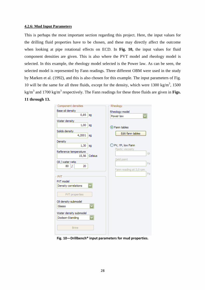
4.2.6: Mud Input Parameters
This is perhaps the most important section regarding this project. Here, the input values for
the drilling fluid properties have to be chosen, and these may directly affect the outcome
when looking at pipe rotational effects on ECD. In Fig. 10, the input values for fluid
component densities are given. This is also where the PVT model and rheology model is
selected. In this example, the rheology model selected is the Power law. As can be seen, the
selected model is represented by Fann readings. Three different OBM were used in the study
by Marken et al. (1992), and this is also chosen for this example. The input parameters of Fig.
10 will be the same for all three fluids, except for the density, which were 1300 kg/m3, 1500
kg/m3 and 1700 kg/m3 respectively. The Fann readings for these three fluids are given in Figs.
11 through 13.
Fig. 10—Drillbench® input parameters for mud properties.

29
Fig. 11—Fann readings used as rheology model input with fluid density of 1300 kg/m3.
Fig. 12—Fann reading used as rheology model input with fluid density of 1500 kg/m3
Fig. 13—Fann reading used as rheology model input with fluid density of 1700 kg/m3
4.2.7: Temperature Input Parameters
Values for temperature parameters were chosen to be found from models within the
Drillbench® software. The surface temperature model on the platform was chosen to be
calculated from a heat loss constant of 40, and an initial pit temperature of 298.15 °K. For
other sections of the well, a dynamic temperature model was chosen to be calculated from the
initial mud temperature by usage of the geothermal gradient.
4.3: Results of Drillbench® Simulations
There is no description of the equations used to calculate the contribution of pipe rotation to
ECD in Drillbench®. However, it is possible to get a plot of the ECD changes versus rotation
speed. To make the Drillbench® example as close as possible to the field study it is based on,
this plot is made for all three mud weights. The sequence of the operations it simulates is also
found from the study of Marken et al. (1992).
For the 1300 kg/m3 mud, the flow rate is 0.030 m3/s, and this rate is kept constant. Before a
simulation is possible, a value for torque had to be chosen, and this was set to 10000Nm. The
rate of penetration was kept at 0, and the inlet temperature was chosen to be 15.56°C. A time
of 2 minutes was chosen for each rotation velocity, and the rotation velocities were chosen to
start on 0 RPM, and have a 5 RPM increment until it reached 600 RPM. The total time of the
“operation” would then be 242 minutes. Fig. 14 shows the ECD variation versus time.
30
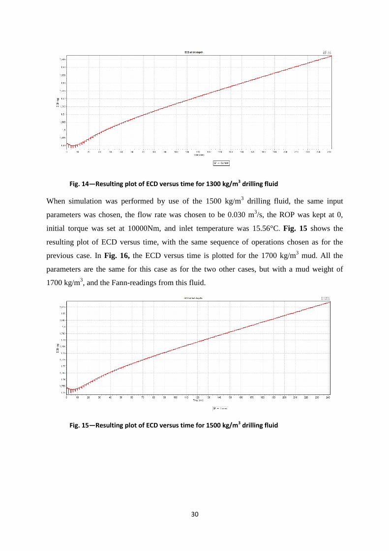
Fig. 14—Resulting plot of ECD versus time for 1300 kg/m3 drilling fluid
When simulation was performed by use of the 1500 kg/m3 drilling fluid, the same input
parameters was chosen, the flow rate was chosen to be 0.030 m3/s, the ROP was kept at 0,
initial torque was set at 10000Nm, and inlet temperature was 15.56°C. Fig. 15 shows the
resulting plot of ECD versus time, with the same sequence of operations chosen as for the
previous case. In Fig. 16, the ECD versus time is plotted for the 1700 kg/m3 mud. All the
parameters are the same for this case as for the two other cases, but with a mud weight of
1700 kg/m3, and the Fann-readings from this fluid.
Fig. 15—Resulting plot of ECD versus time for 1500 kg/m3 drilling fluid

31
Fig. 16—Resulting plot of ECD versus time for 1700 kg/m3 drilling fluid
These graphs provide the values needed for comparison with the empirical equation on the
form ΔPω≠0/ΔPω=0 vs. RPM developed in chapter 5. How this is done will be presented in this
chapter.

32

33
Chapter 5: Development of Own Models Through Regression Analysis This part of the report is where the empirical equations will be derived. The chapter will also
present how the data sets were generated, how the data were prepared to do the regression
analysis, general curve fittings theory will be given, and the accuracy of the equations will be
tested by comparison to simulation results, calculations by usage of the PLR-equation from
chapter 3, and an independent field study.
5.1: Data Sets Generation
One of the main challenges with this project was to generate the data sets. There are not much
public data, and the data sets that are available have to be organized to be used in the
regression analysis. This fact lead to two weaknesses with the equations, they are made from
few data points, and there are no possibilities for gathering more information regarding the
data sets to improve the accuracy of these data points.
To make the regression analysis as precise as possible, the data sets were collected and sorted
in groups. One of the groups was data on the form pressure losses with rotation / pressure
losses without rotation (ΔPω≠0/ΔPω=0) vs. revolutions per minute (RPM). In the study by
Delwiche et al. (1992), pressure data versus rotation rate was studied by Total and DB
Stratabit Ltd (DBS). This data was collected for three different situations of a slim-hole well.
The data in this study was presented on the form ωR/U (dimensionless ratio between rod
tangential velocity and mud axial averaged velocity). Here, ω [rad/s] is the angular rod
rotation speed, R [m] is the rod radius, and U [m/s] is the axial averaged velocity. When data
was collected from this study, this dimensionless number had to be converted to RPM. Data
was available for three different situations.
The first situation, called 578P1172, represents data from a well drilled to a depth of 1180
meters, with a 6.625-in. casing set at 937 meters, and with an openhole diameter of 5.875 in.
for the remaining interval. The drillpipe used had an outer diameter of 5 in. The data was
collected from Fig. 22 replicated in Appendix A, and the result is listed in Table 1. The
rotation speed was converted from ωR/U to RPM with R=ODpipe/2=0.0635 m, and U=0.5 m/s.

34
Table 1—Pressure losses vs. RPM data from 578P1172. DBS on the left side, Total on the right side. ΔPω≠0/ΔPω=0 RPM
ΔPω≠0/ΔPω=0 RPM 1.137 58.4 1.355 58.4 1.218 74.5 1.513 74.5 1.209 84.6 1.272 84.6 1.257 96.0 1.436 96.0 1.230 109.4 1.331 109.4 1.237 109.5 1.558 109.5 1.287 129.3 1.699 129.3 1.310 141.7 1.454 141.7 1.325 141.7 1.510 141.7 1.406 173.2 1.630 173.2 1.406 211.5 1.534 211.5 1.615 261.1 1.842 261.1
The second situation, called 425P1210, contains data from the same well, only now drilled to
a depth of 1214 meters, with a 5-in. casing set at this depth. The drillpipe used had an outer
diameter of 3.7 in. The data was read from Fig. 25 replicated in Appendix A, and the resulting
data points are here listed in Table 2. The rotation speed was converted to RPM by use of
R=ODpipe/2=0.047 m, and U=0.5 m/s.
Table 2—Pressure losses vs. RPM data from 425P1210. DBS data to the left, Total to the right. ΔPω≠0/ΔPω=0 RPM
ΔPω≠0/ΔPω=0 RPM 1.057 30.015 1.071 30.015 1.043 33.478 1.029 33.478 1.086 43.868 1.043 43.868 1.100 58.875 1.050 58.875 1.100 58.875 1.179 58.875 1.129 70.419 1.179 70.419 1.186 87.735 1.121 87.735 1.186 87.735 1.214 87.735 1.186 87.735 1.271 87.735 1.243 105.051 1.250 105.051 1.207 117.750 1.264 117.750 1.264 117.750 1.479 117.750 1.300 132.757 1.357 132.757 1.250 140.838 1.443 140.838 1.250 146.610 1.336 146.610 1.286 177.779 0.979 177.779 1.300 177.779 1.500 177.779 1.343 177.779 1.650 177.779 1.500 177.779 1.707 177.779 1.350 220.493 1.600 220.493 1.393 236.654 1.871 236.654 1.529 265.515 2.029 265.515 1.500 295.529 2.014 295.529 1.621 354.405 1.221 354.405 2.429 354.635 2.286 354.635 1.786 437.522 2.229 437.522 2.200 525.257 1.386 525.257

35
The third situation is called 425P2078. Here, a well was drilled to a depth of 2078 meters. A
5-in. casing string was set at a depth of 1214 meters, and the open hole section down to 2078
meters had a diameter of 4¼ in. The outer pipe diameter was 3.7 in. The data was read from
Fig. 28 replicated in Appendix A, and the resulting data points are listed in Table 3. The
rotation speed was converted to RPM by use of R=ODpipe/2=0.047 m, and U=0.5 m/s.
Table 3—Pressure losses vs. RPM data from well 425P2078. DBS to the left, Total to the right.
ΔPω≠0/ΔPω=0 RPM
ΔPω≠0/ΔPω=0 RPM 2.067 181.627 2.000 181.627 2.117 212.412 2.163 212.412 2.221 261.667 2.150 261.667 2.263 277.059 2.329 277.059 2.358 323.235 2.508 323.235 2.346 332.471 2.142 332.471 2.492 395.579 2.617 395.579 2.571 463.304 2.350 463.304 2.675 507.941 2.592 507.941 2.825 711.118 2.842 711.118
Haige et al. (2000) presented a study of annular pressure losses in a slimhole well. The well
where the measurements were done is called Miao 1-40. In this study, they looked at the
effect of drillpipe rotation on annular pressure losses, and presented the results as can be seen
in Fig. 30 of Appendix B. To make this data useful, it had to be converted to the same form as
for the previous study presented, pressure losses with rotation / pressure losses without
rotation (ΔPω≠0/ΔPω=0) vs. revolutions per minute (RPM). This was done simply by dividing
the given pressure gradients for the various rotation speeds with the pressure gradient of no
rotation. The result for three scenarios are presented in Table 4, case 1 contained data
collected with a velocity of 0.532 m/s, case 2 with a velocity of 0.802 m/s, and case 3 was for
a mud velocity of 1.15 m/s.
Table 4—Pressure losses vs. RPM from Miao 1-40 well. Case 1 to the left, case 2 in the middle, and case 3 to the right.
ΔPω≠0/ΔPω=0 RPM
ΔPω≠0/ΔPω=0 RPM
ΔPω≠0/ΔPω=0 RPM 1.014 30 0.978 30 0.974 30 1.034 70 1.022 70 1.008 70 1.103 110 1.087 110 1.026 110 1.179 150 1.087 150 1.110 150
In a study by Diaz et al. (2004), data from a casing drilling operation collected by MoBPTeCh
Alliance from the Baker Hughes Experimental Test Area (BETA) was presented. In this
study, the accuracy of several theoretical models for calculating ECD were compared to

36
measured data. This was done with three different drilling fluids, water, Mud A and Mud B.
The results was presented as RPM versus bottomhole pressure (BHP), as can be seen in Fig.
33 through Fig. 41 of Appendix C. To make the measured data useful for this project, several
calculations had to be made. For each of the three drilling fluids, ESD was calculated from its
given densities, and the data read from the plots could be made on the form ΔP by subtracting
ESD. By comparing ΔP with rotation to ΔP without rotation, the numbers would be on the
desired form, ΔPω≠0/ΔPω=0 vs. RPM. For each of the three drilling fluids, three sets of data
were measured in the study, with a variation in the pump rate, 0.022 m3/s, 0.028 m3/s and
0.035 m3/s. The data was treated in the same manner as already mentioned for each of these
situations, and the result can be seen in Table 5, Table 6 and Table 7. Table 5 represent the
data measured with water as the drilling fluid, and a density of 998.15 kg/m3 for each of the
three flow rates. The depth of this well section was 86.26 m, with a wellbore diameter of
12.715 in., and an outer casing diameter of 11.75 in.
Table 5—Data of pressure losses vs. RPM collected from BETA. Water as the drilling fluid, Q=0.022 m3/s to the left, Q=0.028 m3/s in the middle, and Q=0.035 ms/s to the right.
ΔPω≠0/ΔPω=0 RPM
ΔPω≠0/ΔPω=0 RPM
ΔPω≠0/ΔPω=0 RPM 1.265 60 1.073 60 1.121 60 1.088 120 1.215 120 1.301 120 1.941 180 1.035 180 1.462 180
Table 6 represent the data measured in the same well, but with Mud A (a bentonite/water
mixture) as drilling fluid. The density of the drilling fluid was 1042.49 kg/m3, the depth was
86.26 m, with a wellbore diameter of 12.715 in., and a casing diameter of 11.75 in.
Table 6—Data of pressure losses versus RPM collected from BETA. Mud A as the drilling fluid, Q=0.022 m3/s to the left, Q=0.028 m3/s in the middle, and Q=0.035 m3/s to the right. No data was found above 120 RPM for Q=0.022 m3/s.
ΔPω≠0/ΔPω=0 RPM
ΔPω≠0/ΔPω=0 RPM
ΔPω≠0/ΔPω=0 RPM 1.449 60 1.147 60 0.963 60 1.296 120 1.172 120 1.023 120 xxxx xxxx 0.824 180 0.731 180
Table 7 contains data measured in the same well as previously described, but with Mud B (a
bentonite/water mixture) as drilling fluid. As for the previous cases, the depth was 86.26 m,
the wellbore diameter was 12.715 in., and the outer casing diameter was 11.75 in. The density
of Mud B was found to be 1174.30 kg/m3.

37
Table 7—Data of pressure losses versus RPM collected from BETA. Mud B as the drilling fluid, Q=0.022 m3/s to the left, Q=0.028 m3/s in the middle, and Q=0.035 m3/s to the right.
ΔPω≠0/ΔPω=0 RPM
ΔPω≠0/ΔPω=0 RPM
ΔPω≠0/ΔPω=0 RPM 1.335 60 0.920 60 0.921 60 1.646 120 1.196 120 1.036 120 2.508 180 1.437 180 1.251 180
In the study by Hemphill et al. (2007), well data from two tests carried out on the 22/30c-G4
well at the Elgin-Franklin UKCS fields were presented. The data were presented as measured
change in ECD (lbm/gal) vs. drillpipe rotation speed (RPM), and consequently, the data had
to be converted to the form pressure losses with rotation / pressure losses without rotation
(ΔPω≠0/ΔPω=0) vs. revolutions per minute (RPM) to compare them with the other data sets
collected. In this study, it was referred to a study by Isambourg et al. (1999) for further
details, and this is the source of the parameters used in the conversion process. After the data
points for the two tests (Elf 8.75-in A and Elf 8.75-in B) had been found, the values for
measured change in ECD (lbm/gal) was converted to measured change in ECD (kg/m3). The
ECD with no pipe rotation was found to be 2233 kg/m3, while the ESD was found to be 2190
kg/m3; hence the ECD increase with no rotation was 43 kg/m3. By dividing the converted data
points with this ECD increase, all data was on the required form. The data points on the final
form are presented in Table 8, and a copy of the original source can be found in Fig. 43 of
Appendix E.
Table 8—Welldata from the 22/30c-G4 well, test Elf 8.75-in A to the left, and Elf 8.75-in B to the right.
ΔPω≠0/ΔPω=0 RPM
ΔPω≠0/ΔPω=0 RPM 0.121 60 0.224 60 0.407 120 0.447 120 0.468 150 0.700 180 0.606 180
For the second type of empirical equations predicting pressure losses caused by drillpipe
rotation, it was decided that more consideration had to be given to the well characterizations
and the fluid behavior. To do this, the Reynolds number was chosen to be used as the basis of
the equations. The data sets were collected on the form ΔPω≠0/ΔPω=0 vs. Reynolds number,
and consequently, equations had to be made for several rotation speeds.
After a process of gathering possible data sets, three rotation speeds were found to have a
large enough number of data points to do the regression analysis. These rotation speeds were
200 RPM, 300 RPM and 600 RPM. The first data points that could be converted to the

38
required form were found from the study of Delwiche et al. (1992). In well 578P1172,
described in detail earlier in this chapter, measurements of the pressure losses were done at a
variety of mud flow rates for a pipe rotation speed of 200 RPM, as seen in Fig. 23 of
Appendix A. This data had to be converted to get it in on the form ΔPω≠0/ΔPω=0 vs. Reynolds
number. The pressure loss data was converted to ΔPω≠0/ΔPω=0 data by dividing the pressure
loss value at 200 RPM with the value for that of no rotation. To get the mud flow expressed
by the Reynolds number, the flow rate had to be converted to mud velocity by dividing it with
the flow area of the annulus, and then the Reynolds numbers were calculated with the general
equation for Reynolds number:
Reeff
vdρµ
= (5.1)
The rheology model that best fitted this measurement was the Power law; hence the values for
μeff were calculated from the equation representing effective viscosity in annulus for the
Power law model:
12 2 13 12
n
heff
h
Kdv nd n v
µ +
= ⋅ ⋅
(5.2)
All input data for the calculations can be found in Table 27 of Appendix H, along with a copy
of the original source for the data sets. The final data points are presented in Table 9.
Table 9—Welldata from 578P1172 on the form ΔPω≠0/ΔPω=0 vs. Reynolds number, RPM=200
ΔPω≠0/ΔPω=0 Re 1.475 184 1.389 303 1.479 432 1.353 569
In the same study, data points were collected from well 425P1210 for 200 RPM (see Fig. 26
of Appendix A). The same conversions had to be made on these data points, and the input
values for the calculations can be found in Table 28 of Appendix H. The final data points are
presented in Table 10.
Table 10—Welldata from 425P1210 on the form ΔPω≠0/ΔPω=0 vs. Reynolds number, RPM=200
ΔPω≠0/ΔPω=0 Re 1.286 10 1.800 23 1.460 39 1.247 56 1.174 74 1.059 93

39
Bode et al. (1989), presented a study of a test well called SHADS #7. This well was drilled
down to 609.6 m, with a 5-in. casing and a 3.7-in. drillstring. Measurements of the annular
pressure loss with rotation to that without rotation was plotted against the Reynolds number
for a rotation speed of 200 RPM, as can be seen in Fig. 42 of Appendix D. The resulting data
set can be seen in Table 11.
Table 11—Welldata from SHADS #7 testwell on the form ΔPω≠0/ΔPω=0 vs. Reynolds number, 200 RPM rotation speed.
ΔPω≠0/ΔPω=0 Re 1.673 426 1.684 721 2.220 971 1.724 1103 1.704 1471 1.857 1574 1.551 2217 1.796 2348 1.404 2913 1.531 3382 1.319 3632 1.245 4391 1.394 4478 1.298 5632 1.255 6841
In the study by Delwiche et al. (1992), data from well 425P2078 was presented in the same
manner as for the two other wells from this study (see Fig. 29 of Appendix A), and the same
conversions had to be made on this data set to make it useful. The input for the calculations
that was performed can be found in Table 29 of Appendix H, and a summary of the data
points are presented in Table 12. The rotation speed in this measurement was 300 RPM.
Table 12—Welldata from 425P2078 on the form ΔPω≠0/ΔPω=0 vs. Reynolds number, rotation speed was 300 RPM.
ΔPω≠0/ΔPω=0 Re 2.143 57 1.917 86 2.042 117 1.967 149 1.939 183
McCann et al. (1993) studied how ECD was affected by drillpipe rotation in a slimhole test
well called SHDT.1. They measured the ECD increase at different flow rates for a rotation
rate of 300 RPM, presented in Fig. 44 of Appendix F. This data set had to be converted to get
it on the required form. The Reynolds numbers were calculated for several flow rates, by use
of the general form of Reynolds number, and the effective viscosity was calculated from the

40
Newtonian model because water was used as drilling fluid. All calculation input can be found
in Table 30 of Appendix H, and the resulting data set is given in Table 13.
Table 13—Welldata from SHDT.1 testwell on the form ΔPω≠0/ΔPω=0 vs. Reynolds number, pipe rotation was 300 RPM
ΔPω≠0/ΔPω=0 Re 1.818 298 1.588 398 1.565 497 1.533 597 1.400 696 1.420 796 1.317 895 1.316 995 1.289 1094 1.260 1194 1.233 1293
In the same study by McCann et al. (1993), they measured the ECD increase for different
flow rates with a rotation speed of 600 RPM in the same well. These measurements were
presented in the same way as with the 300 RPM rotation speed (see Fig. 44 of Appendix F),
and consequently the same conversions had to be made. The input values from these
calculations can be found in Table 30 of Appendix H, and the resulting data set is given in
Table 14.
Table 14—Welldata from SHDT.1 testwell on the form ΔPω≠0/ΔPω=0 vs. Reynolds number, rotation speed was 600 RPM
ΔPω≠0/ΔPω=0 Re 2.545 298 2.118 398 2.000 497 1.900 597 1.750 696 1.680 796 1.587 895 1.487 995 1.456 1094 1.423 1194 1.392 1293
In the study by Bode et al. (1989) earlier described, it was also done measurements of the
annular pressure losses with rotation over the annular pressure losses without rotation for a
rotation speed of 600 RPM on the SHADS #7 test well, as seen in Fig. 42 of Appendix D. All
well parameters were the same for this test as with the one using a rotation speed of 200
RPM. A presentation of the final data set can be found in Table 15.

41
Table 15—Welldata from SHADS #7 testwell on the form ΔPω≠0/ΔPω=0 vs. Reynolds number, rotation speed is 600 RPM
ΔPω≠0/ΔPω=0 Re 1.837 426 2.060 721 2.860 971 2.170 1103 2.130 1471 2.510 1574 2.110 2217 2.590 2348 1.867 2913 2.140 3382 1.745 3632 1.633 4391 1.929 4478 1.857 5632 1.653 6841
5.2: Resulting Regressed Equations
From the data sets presented in the previous subchapter, empirical equations describing the
effect of pipe rotation on the annular pressure drop and ECD was developed. The first
equation was found with the data sets on the form ΔPω≠0/ΔPω=0 vs. RPM. All the data was
gathered in one Excel sheet, and plotted against each other. From this plot, a best-fit line was
selected, along with the equation describing this line, and the R2-value. The R2-value is a
statistical value describing how well the regressed line approximates to the real data points. It
ranges from 0 to 1, and the closer it is to 1, the better the approximation. As can be seen in the
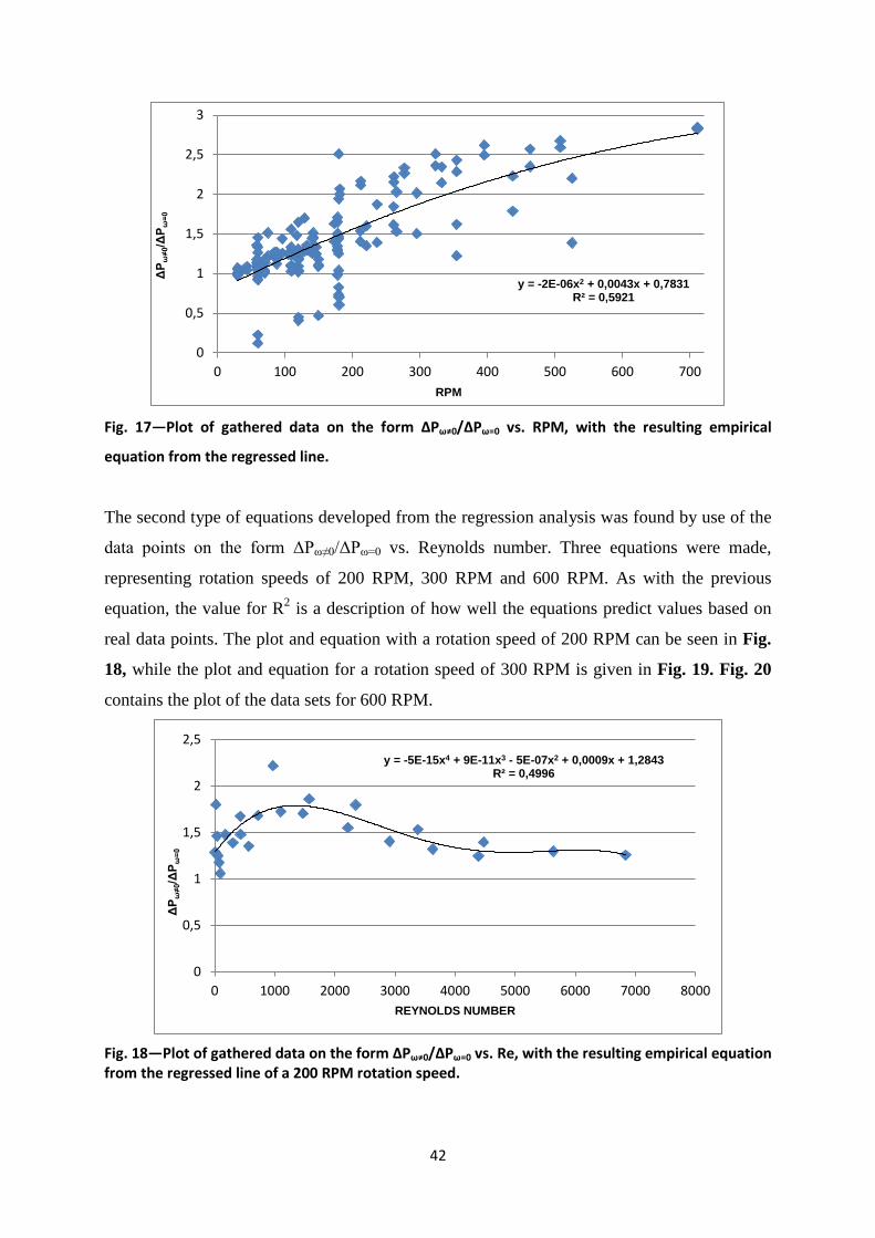
resulting graph presented in Fig. 17, the R2 value is 0.5921. The empirical equation found
was:
22 06 0,0043 0,7831y E x x= − − + + (5.3)
In this equation, y represents ΔPω≠0/ΔPω=0, and x represents RPM. In the next part of this
subchapter, the accuracy of this equation will be tested against Drillbench® simulations, a
field study that was not used in the regression analysis, and the equation presented in chapter
3, called the PLR-equation.
42
Fig. 17—Plot of gathered data on the form ΔPω≠0/ΔPω=0 vs. RPM, with the resulting empirical
equation from the regressed line.
The second type of equations developed from the regression analysis was found by use of the
data points on the form ΔPω≠0/ΔPω=0 vs. Reynolds number. Three equations were made,
representing rotation speeds of 200 RPM, 300 RPM and 600 RPM. As with the previous
equation, the value for R2 is a description of how well the equations predict values based on
real data points. The plot and equation with a rotation speed of 200 RPM can be seen in Fig.
18, while the plot and equation for a rotation speed of 300 RPM is given in Fig. 19. Fig. 20
contains the plot of the data sets for 600 RPM.
Fig. 18—Plot of gathered data on the form ΔPω≠0/ΔPω=0 vs. Re, with the resulting empirical equation from the regressed line of a 200 RPM rotation speed.
y = -2E-06x2 + 0,0043x + 0,7831 R² = 0,5921
0
0,5
1
1,5
2
2,5
3
0 100 200 300 400 500 600 700
ΔP ω
≠0/ΔP ω
=0
RPM
y = -5E-15x4 + 9E-11x3 - 5E-07x2 + 0,0009x + 1,2843 R² = 0,4996
0
0,5
1
1,5
2
2,5
0 1000 2000 3000 4000 5000 6000 7000 8000
ΔP ω
≠0/ΔP ω
=0
REYNOLDS NUMBER

43
Fig. 19—Plot of gathered data on the form ΔPω≠0/ΔPω=0 vs. Re, with the resulting empirical equation from the regressed line of a 300 RPM rotation speed.
Fig. 20—Plot of gathered data on the form ΔPω≠0/ΔPω=0 vs. Re, with the resulting empirical equation from the regressed line of a 600 RPM rotation speed.
As can be seen in Fig. 18, the empirical equation for ΔPω≠0/ΔPω=0 versus Reynolds number for
a rotation speed of 200 RPM is:
15 4 11 3 7 25 10 9 10 5 10 0,0009 1,2843y x x x x− − −= − ⋅ + ⋅ − ⋅ + + (5.4)
The variable y represents ΔPω≠0/ΔPω=0, and x represents the Reynolds number. For this
equation, the R2-value is 0.4996. With this equation, it is possible to predict the additional
pressure losses caused by rotation at a speed of 200 RPM, at given Reynolds numbers. The
same equation for a rotation speed of 300 RPM is given by:
y = 4,7646x-0,184 R² = 0,9433
0
0,5
1
1,5
2
2,5
0 200 400 600 800 1000 1200 1400
ΔP ω
≠0/ΔP ω
=0
REYNOLDS NUMBER
y = -2E-12x3 + 1E-08x2 - 1E-05x + 1,9658 R² = 0,0355
0
0,5
1
1,5
2
2,5
3
3,5
0 1000 2000 3000 4000 5000 6000 7000 8000
ΔP ω
≠0/ΔP ω
=0
REYNOLDS NUMBER

44
0,1844,7646y x−= ⋅ (5.5)
The variables are the same as for the previous equation. R2=0.9433 for this equation, meaning
that it is close to the real data points. For the 600 RPM rotation speed, the equation was found
to be:
12 3 8 2 52 10 1 10 1 10 1,9658y x x x− − −= − ⋅ + ⋅ − ⋅ + (5.6)
The R2-value is 0.0355, and the regressed line is thereby not an accurate prediction of the data
points. The presented equations will be tested against an existing semi-empirical equation,
and against real drilling data from a field study later in this chapter.
5.3: Results
As was seen in Fig. 17, the resulting regressed equation from the data sets on the form
ΔPω≠0/ΔPω=0 vs. RPM predict a substantial pressure loss with increasing rotation speeds. This
is as expected from the data sets gathered, because much of the data used originate from
slimhole drilling, in which rotation of the drillpipe can give as much as 90% of the total
annular pressure losses. However, because larger pressure losses are expected for slimhole
drilling than for conventional drilling, it is expected that this equation will predict a value
above the actual pressure loss ratio. By comparing with the Drillbench® simulation based on
a field study, and the predicted values from the semi-empirical equation presented in chapter
3, it can be seen whether this expectation is fulfilled.
The three regressed equations on the form ΔPω≠0/ΔPω=0 vs. Reynolds number do not have the
same shape, but they have some similarities. The pressure loss with rotation over that without
rotation is decreasing with an increasing Reynolds number. This is as expected because the
mud flow would not be affected as much by pipe rotation for a turbulent flow as for a laminar
flow. These equations will also be compared to Drillbench® simulations and the PLR-
equation from chapter 4, but there is not enough field data to test the accuracy of the
equations by comparing with a dataset not used in the creation of the equations.
5.3.1: Comparison With Drillbench® Simulations
In this section, the regressed equations will be compared to the results of the Drillbench®
simulations done in chapter 4. The first equation to be compared, is the one derived from the
data sets on the form ΔPω≠0/ΔPω=0 vs. RPM. This is done by choosing to look at specific
rotation speeds, and compare the calculated values of the empirical equation with the values

45
obtained in Drillbench® for these rotation speeds. The rotation speeds chosen to be looked at,
are 60 RPM, 120 RPM, 150 RPM, 200 RPM, 400 RPM and 600 RPM. From the figures in
chapter 4 representing the simulation results, it was seen that the plot was ECD versus time.
The time can easily be converted to RPM because a constant time of two minutes was chosen
for every 5 RPM increase. In the Drillbench® software, it is possible to track the values of a
graph, and this was done to find the corresponding ECD value for the 6 rotation speeds.
Because ECD is not the value to be compared, these numbers had to be converted to the form
ΔPω≠0/ΔPω=0. This was done by dividing the sum of the ECD value read from the graph and
ESD (the mud weight in SG), with the sum of ECD with no rotation and the ESD:
0 00
( )/( )
read
RPM
ECD ESDP PECD ESDω ω≠ =
−∆ ∆ =
− (5.7)
These values were calculated by use of the three different mud weights. The comparison with
the approximations from the empirical equation for the 1300 kg/m3 mud is shown in Table
16; the comparison with the 1500 kg/m3 is shown in Table 17, and with the 1700 kg/m3 mud
in Table 18.
Table 16—Comparison of results from simulation and empirical equation, mud weight 1300 kg/m3
RPM ΔPω≠0/ΔPω=0 from Drillbench® ΔPω≠0/ΔPω=0 vs. RPM-equation Difference [%] 60 1.0244 0.9931 −3.06 %
120 1.0634 1.1931 12.19 % 150 1.0801 1.3831 28.05 % 200 1.1061 1.5631 41.32 % 400 1.1992 2.1831 82.05 % 600 1.2845 2.6431 105.78 %
Table 17—Comparison of results from simulation and empirical equation, mud weight 1500 kg/m3
RPM ΔPω≠0/ΔPω=0 from Drillbench® ΔPω≠0/ΔPω=0 vs. RPM-equation Difference [%] 60 1.0208 0.9931 −2.71 %
120 1.0553 1.1931 13.06 % 150 1.0698 1.3831 29.29 % 200 1.0921 1.5631 43.13 % 400 1.1733 2.1831 86.07 % 600 1.2489 2.6431 111.63 %
Table 18—Comparison of results from simulation and empirical equation, mud weight 1700 kg/m3
RPM ΔPω≠0/ΔPω=0 from Drillbench® ΔPω≠0/ΔPω=0 vs. RPM-equation Difference [%] 60 1.0093 0.9931 −1.61 %
120 1.0420 1.1931 14.50 % 150 1.0533 1.3831 31.31 % 200 1.0708 1.5631 45.97 % 400 1.1349 2.1831 92.35 % 600 1.1947 2.6431 121.24 %

46
As can be seen from these tables, the difference between the predicted result by use of the
ΔPω≠0/ΔPω=0 vs. RPM-equation and the Drillbench® simulation is increasing with increasing
rotation rate for all three mud weights. Either the equation is predicting a too large pressure
loss for high rotation speeds, or the software is predicting too low values. By comparing with
the PLR-equation and a field study in the next subchapter, an answer to this will be found.
To test the equations on the form ΔPω≠0/ΔPω=0 versus Reynolds number, simulations in
Drillbench® had to be made based on the Reynolds number. This is not a parameter that can
be chosen, so it had to be found by modifying the input parameters according to equation
(5.1). Two values were chosen to be tested, Re=500 and Re=4000. These values were chosen
to get both a laminar and a turbulent flow situation. The Drillbench® simulations were done
based on the example of a 1500 kg/m3 drilling fluid presented in chapter 4. With input
parameters from this example, the Reynolds number of 500 was found by changing the flow
rate to 0.006 m3/s, while a Reynolds number of 4000 was found at a flow rate of 0.050 m3/s.
The other parameters were kept the same. By reading the values for ECD at rotation rates of
200 RPM, 300 RPM and 600 RPM, and converting these values to the form ΔPω≠0/ΔPω=0 by
use of Eq. 5.7, they could be compared to the empirical equations. The result can be seen in
Table 19 for a Reynolds number of 500, and in Table 20 for a Reynolds number of 4000.
Table 19—Comparison of Drillbench® simulation and ΔPω≠0/ΔPω=0 vs. Re-equations for laminar flow. Reynolds number = 500 (Laminar flow)
RPM Drillbench® prediction of ΔPω≠0/ΔPω=0
Prediction of ΔPω≠0/ΔPω=0 from empirical equations Difference
200 0.96524 1.62024 67.86 % 300 0.95588 1.51850 58.86 %
600 0.89706 1.96305 118.83 %
Table 20—Comparison of Drillbench® simulation and ΔPω≠0/ΔPω=0 vs. Re-equations for turbulent flow. Reynolds number = 4000 (Turbulent flow)
RPM Drillbench® prediction of ΔPω≠0/ΔPω=0
Prediction of ΔPω≠0/ΔPω=0 from empirical equations Difference
200 1.07205 1.36430 27.26 % 300 1.10886 1.03573 −6.59 %
600 1.21536 1.95780 61.09 %
From these two tables, it can be seen that the predictions with the empirical equations are
closer to the Drillbench® simulation results than was the case for the regressed equation on
the form ΔPω≠0/ΔPω=0 vs. RPM, but the prediction is still higher in general.

47
5.3.2: Comparison With PLR-Equation and a Field Study
This subchapter will compare the results of the regressed equations with the PLR-equation
presented in chapter 3, and with the results from the study by Marken et al. (1992), in which
the Drillbench® example was based on. In this study, pressure losses in the well at drillstring
rotation speeds of 60 RPM and 120 RPM were investigated. As previously described, they
used three different mud weights, and made several measurements for all the scenarios. When
rotating at 60 RPM, the ratio of the annular pressure losses with rotation to that without
rotation ranged between 1.11 and 1.51. At the rotation speed of 120 RPM, the same ratio was
between 1.18 and 1.67.
To make use of the PLR-equation, several calculations had to be made. A summary of these
calculations can be found in Appendix G. Some of the values had to be assumed because the
study provided insufficient information, and these values were the ones related to the
eccentricity. It was recommended to use a value of 50%, so this was assumed to be a fair
estimate for the calculation. The n-variable was calculated by use of the Herschel-Bulkley
rheology model, and a log-log plot from a 3 data point oil field approach. Table 21 contain
the calculated values of ΔPω≠0/ΔPω=0 for 60 RPM and 120 RPM, for the three different mud
weights.
Table 21—ΔPω≠0/ΔPω=0 vs. RPM–equation compared to PLR-equation and field study.
RPM Mud weight [kg/m3] ΔPω≠0/ΔPω=0 PLR ΔPω≠0/ΔPω=0 range from study 60 1300 0.9931 1.3421 1.11–1.51 60 1500 0.9931 1.3224 1.11–1.52 60 1700 0.9931 1.2971 1.11–1.53
120 1300 1.1931 1.4028 1.18–1.67 120 1500 1.1931 1.3823 1.18–1.68 120 1700 1.1931 1.3384 1.18–1.69
As previously mentioned, there are not enough field data to test the equations on the form
ΔPω≠0/ΔPω=0 versus Reynolds number against a field study not used in the regression analysis.
The study that was used for comparison with the equation on the form ΔPω≠0/ΔPω=0 vs. RPM
did not use rotation speeds above 120 RPM, and is thereby unfitted for verification purposes.
However, the PLR-equation can be used. To calculate the required pressure loss ratios, the
same input values used in the previous comparison for a 1500 kg/m3 mud was applied. Two
situations were looked at, a laminar flow situation (Re=500), and a turbulent flow situation
(Re=4000). The resulting comparison can be seen in Table 22 and Table 23.
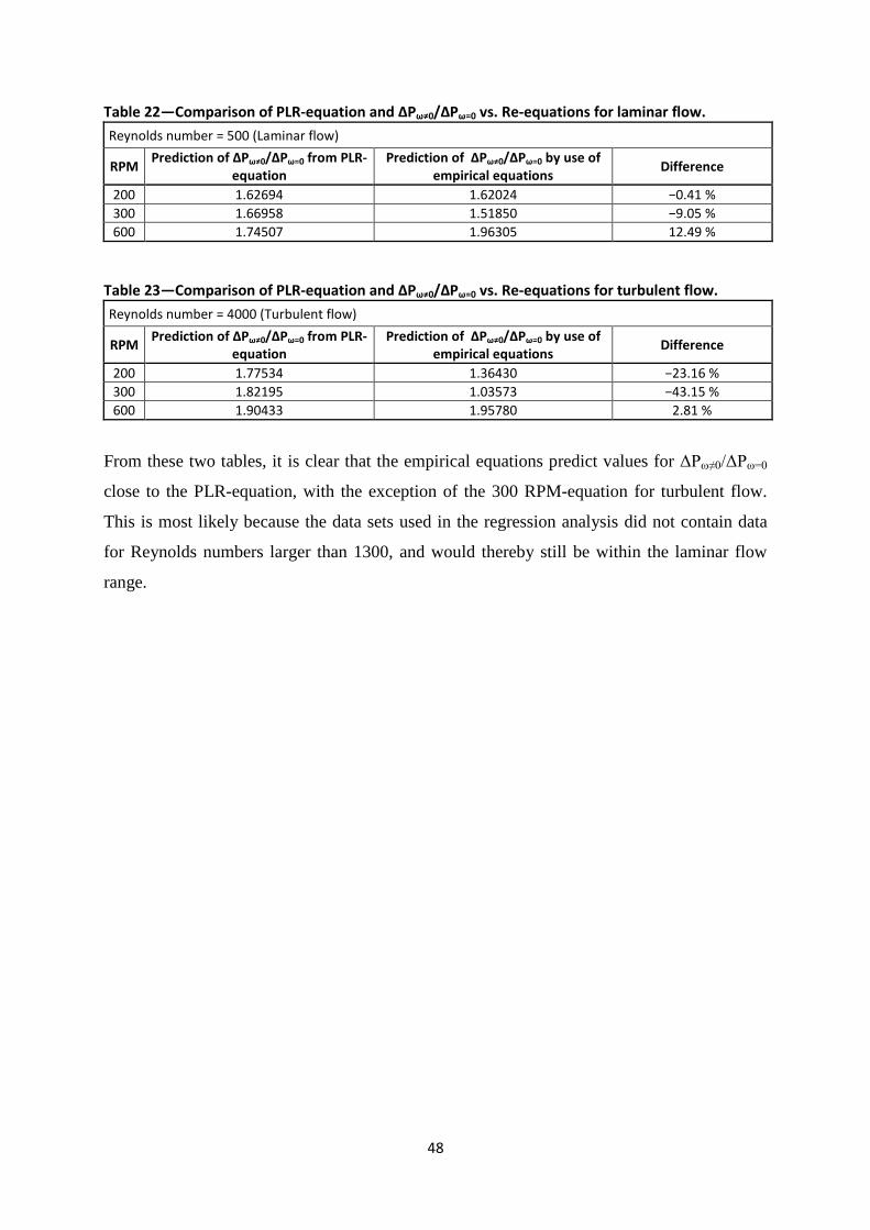
48
Table 22—Comparison of PLR-equation and ΔPω≠0/ΔPω=0 vs. Re-equations for laminar flow. Reynolds number = 500 (Laminar flow)
RPM Prediction of ΔPω≠0/ΔPω=0 from PLR-equation
Prediction of ΔPω≠0/ΔPω=0 by use of empirical equations
Difference
200 1.62694 1.62024 −0.41 % 300 1.66958 1.51850 −9.05 % 600 1.74507 1.96305 12.49 %
Table 23—Comparison of PLR-equation and ΔPω≠0/ΔPω=0 vs. Re-equations for turbulent flow. Reynolds number = 4000 (Turbulent flow)
RPM Prediction of ΔPω≠0/ΔPω=0 from PLR-equation
Prediction of ΔPω≠0/ΔPω=0 by use of empirical equations
Difference
200 1.77534 1.36430 −23.16 % 300 1.82195 1.03573 −43.15 % 600 1.90433 1.95780 2.81 %
From these two tables, it is clear that the empirical equations predict values for ΔPω≠0/ΔPω=0
close to the PLR-equation, with the exception of the 300 RPM-equation for turbulent flow.
This is most likely because the data sets used in the regression analysis did not contain data
for Reynolds numbers larger than 1300, and would thereby still be within the laminar flow
range.

49
Chapter 6: Discussion and Evaluation of Work The empirical equations developed in the previous chapters have some limitations. They are
made from a small amount of data sets, and do not represent a large enough spread. The data
sets are gathered from previous studies on effects of pipe rotation.
6.1 Data Quality
Some errors could have been made in the measurements during the tests, the equipment could
have been inaccurately calibrated, or there could have been other factors such as different test
conditions for the various runs that would influence the results. A factor that could affect the
accuracy of the equations is poorly read data from graphs. There will always be an error when
reading values from a graph and the size of each point indicator or the thickness of the line
may also influence the read values. The downhole pressure is assumed to be the same as
standpipe pressure plus hydraulic pressure, and only the annulus pressures considered. This
might also influence the results. The rheology model is a mathematical expression on mud
behavior, and does not necessarily depict the actual behavior, although the model that best fits
measurements on the mud has been chosen.
6.2 Model Quality
The models were constricted into two types, to fit data representing ΔPω≠0/ΔPω=0 versus
RPM, and model to fit data representing ΔPω≠0/ΔPω=0 versus the Reynolds number. Four
equations were found, and these equations were tested against simulations in Drillbench®,
against a semi-empirical equation from a previous study (Ahmed et al. 2010) on pipe rotation,
and for the equation of ΔPω≠0/ΔPω=0 versus RPM, it was tested against data from an
independent study.
As can be seen in the figures with the regressed model lines (fig. 17 through fig. 20), there are
a great variety in the data points, and consequently the model lines are not accurate for all
data points. This is also reflected by the R2-value, which is as low as 0.0355 for the equation
describing pressure losses versus Reynolds number for a pipe rotation speed of 600 RPM. The
best value of R2 was seen for the equation of pressure losses versus pipe rotation speed of 300
RPM, where the value was 0.9433. These values reflect how well the model line fits the data
points used in the regression analysis, and therefore may not be a true reflection on the
accuracy of the equation when tested against other field data. This was also seen in the

50
comparison of the 300 RPM-equation with the PLR-equation, where the largerst deviation
appeared.
The difference between model output on the form ΔPω≠0/ΔPω=0 versus RPM was −1.61% at
the minimum, with a rotation speed of 60 RPM and a mud weight of 1700 kg/m3, while the
largest difference was found to be +121.24% with a rotation rate of 600 RPM and the same
mud weight. In general, the difference increased with increasing rotation rate for all mud
weights.
The equations on the form ΔPω≠0/ΔPω=0 versus Reynolds number gave a large difference for
both a laminar flow (Re=500) and a turbulent flow (Re=4000) with the exception of the
equation for a rotation speed of 300 RPM. This predicted a pressure loss ratio with a
difference of −6.59% compared to the Drillbench® result for the case of turbulent flow. This
is thought to be due to the fact that the data points used in the regression analysis of this
rotation speed does not cover Reynolds numbers in the range of turbulent flow.
The ΔPω≠0/ΔPω=0 vs. RPM-equation correlated better with the equation from the study
presented in chapter 3, but generally predicted too low pressure losses. The equations on the
form ΔPω≠0/ΔPω=0 versus Reynolds number gave satisfying results compared with the
predictions from the semi-empirical equation presented in chapter 3, but predicted smaller
losses for both laminar and turbulent flow (Re=500 and Re=4000) for rotation speeds of 200
RPM and 300 RPM. The difference increased for both equations when the Reynolds number
was 4000. The equation for a rotation rate of 600 RPM gave the best results. This predicted a
pressure loss 12.49% above the result found using the equation presented in chapter 3 for the
laminar flow, while the difference was only +2.81% for the turbulent flow.
6.3 Future Improvements
All equations developed in present project gave predictions of ECD changes due to pipe
rotation closer to field data and already existing equations than the software used in this
project. However, the results are not yet satisfying as a simple approach to predict pressure
losses. There is a need for more data sets to cover a larger variety of drilling operations and
situations, and further testing is still needed. From present project it seems to be hard to get a
prediction of pressure losses with the required quality, because there are too many parameters

51
that will influence the pressure losses, such as eccentricity, borehole diameter, what drill fluid
is used, and what flow situation exists.
By gathering larger data sets covering more situations, the equations found in this project can
be further developed to reach a final form with predictions close to field measurements. The
equations on the form ΔPω≠0/ΔPω=0 versus Reynolds number require less input values than
existing equations, but does not cover enough rotation speeds, so a set of equations covering
all situations cannot be made without more time and available data.
The models developed in present project are simple. A more complex model should be
considered. This model should be made based on the individual variables, where the final
form of the model will be on a multi-variable form when the collected data sets allow this to
happen. A model of this type would predict pressure losses more accurately, but still be on a
simple form. For this to happen there is a need for larger data sets, and more time.

52
53
Chapter 7: Conclusion On basis of findings and observations made during the present project work, the following
conclusions can be drawn:
1. The newest relevant theory has been studied to get an overview of existing knowledge.
Areas in need of improvement have been found, and the foundation for a best practice
recommendation is set.
2. Four equations was developed based on the data sets gathered in present project. The
equations was made through regression analysis of data sets on the simlpe model form
ΔPω≠0/ΔPω=0 versus RPM, and ΔPω≠0/ΔPω=0 versus Reynolds number.
3. Equations developed in present project were tested for their accuracy against
simulations performed in Drillbench®, against a semi-empirical equation, and against
an independent field study.
4. Our model on the form ΔPω≠0/ΔPω=0 versus RPM was found to predict pressure losses
well, and close to the result of the semi-empirical equation. Our model predicted
higher pressure losses for most rotation speeds compared to the Drillbench®
simulation results.
5. The equations on the form ΔPω≠0/ΔPω=0 versus Reynolds were tested for both a
laminar flow situation (Re=500) and a turbulent flow situation (Re=4000).
6. To improve the accuracy of the developed equations, further gathering of data sets
must be made. There was not a satisfying variation in the data sets. With more data
points, the model can be adjusted with greater confidence.
7. The equations developed in present project did not cover all drilling situations.
Equations on the form ΔPω≠0/ΔPω=0 versus Reynolds number was only developed for
rotation speeds of 200 RPM, 300 RPM, and 600 RPM. To develop equations for more
rotation speeds, more time and field data is necessary.
8. To improve the model, a more complex model should be made. This can be done by
looking at the variables individually, and collect these variables into a multi-variable
model when the data allows for it to happen.

54
55
References
Ahmed, R. and Miska, S. 2008. Experimental Study and Modeling of Yield Power-Law Fluid Flow in
Annuli with Pipe Rotation. Paper IADC/SPE 112604 presented at the IADC/SPE Drilling Conference,
Orlando, Florida, USA, 4–6 March.
Ahmed, R., Enfis, M., and Miftah-El-Kheir, H. et al. 2010. The Effect of Drillstring Rotation on Equivalent
Circulation Density: Modeling and Analysis of Field Measurements. Paper SPE 135587 presented at
the SPE Annual Technical Conference and Exhibition, Florence, Italy, 19–22 September.
Ward, C. and Andreassen, A. 1997. Pressure-While-Drilling Data Improve Reservoir Drilling Performance.
Paper SPE 37588 presented at the SPE/IADC Drilling Conference, Amsterdam, 4–6 March.
Bode, D.J., Noffke, R.B., and Nickens, H.V. 1989. Well-Control Methods and Practices in Small-Diameter
Wellbores. Paper SPE 19526 presented at the SPE Annual Technical Conference and Exhibition, San
Antonio, Texas, USA, 8–11 October.
Charlez, A., Easton, M., and Morrice, G. et al. 1998. Validation of Advanced Hydraulic Modeling using
PWD Data. Paper OTC 8804 presented at the Offshore Technology Conference, Houston, 4–7 May.
Delwiche, R.A., Lejeune, M.W.D and Mawet, P.F.B.N, et al. 1992. Slimhole Drilling Hydraulics. Paper
SPE 24596 presented at the Annual Technical Conference and Exhibition of the Society of Petroleum
Engineers, Washington, DC, 4–7 October.
Diaz, H., Miska, S., and Takach, N. et al. 2004. Modeling of ECD in Casing Drilling Operations and
Comparison with Experimental and Field Data. Paper IADC/SPE 87149 presented at the IADC/SPE
Drilling Conference, Dallas, 2–4 March.
Haige, W., Yinao, S., and Yangmin, B. et al. 2000. Experimental Study of Slimhole Annular Pressure Loss
and Its Field Applications. Paper IADC/SPE 59265 presented at the IADC/SPE Drilling Conference,
New Orleans, 23–25 February.
Hansen, S.A. and Sterri, N. 1995. Drill Pipe Rotation Effects on Frictional Pressure Losses in Slim Annuli.
Paper SPE 30488 presented at the SPE Annual Technical Conference and Exhibition, Dallas, 22–25
October.
Hansen, S.A., Rommetveit, R., and Sterri, N. et al. 1999. A New Hydraulics Model for Slim Hole Drilling
Applications. Paper SPE/IADC 57579 presented at the SPE/IADC Middlie East Drilling Technology
Conference, Abu Dhabi, 8–10 November.
Hemphill, T., Bern, P., and Rojas, J.C. et al. 2007. Field Validation of Drillpipe Rotation Effects on
Equivalent Circulation Density. Paper SPE 110470 presented at the SPE Annual Technical Conference
and Exhibition, Anaheim, California, USA, 11–14 November.

56
Isambourg, P., Brangetto, M., and Bertin, D.L. 1998. Field Hydraulic Tests Improve HPHT Drilling Safety
and Performance. Paper SPE 59527 presented at the SPE Annual Technical Conference and
Exhibition, New Orleans, 27–30 September.
Marken, C.D., He, X. and Saasen, A. 1992. The Influence of Drilling Conditions on Annular Pressure
Losses. Paper SPE 24598 presented at the Annual Technical Conference and Exhibition of the of the
Society of Petroleum Engineers, Washington, DC, 4–7 October.
McCann, R.C., Quigley, M.S., Slater K.S. et al. 1993. Effects of High-Speed Pipe Rotation on Pressure in
Narrow Annuli. Paper SPE 26343 presented at the SPE Annual Technical Conference and Exhibition,
Houston, 3–6 October.
New Mexico Tech University. 2012. Swab/Surge pressures,
http://infohost.nmt.edu/~petro/faculty/Kelly/Swab.pdf (accessed 07 March 2012).
OilGasGlossary. 2012. Oil and Gas Glossary, http://oilgasglossary.com/friction-loss.html (accessed 13
March).
Skalle, P. 2010. Drilling Fluid Engineering. © 2010 Pål Skalle & Ventus Publishing ApS, ISBN 978-87-
7681-552-3. http://bookboon.com/no/laereboker/geoscience-eboker/.
Skjold, T. L. 2011. Report on impact of borehole dynamics on well stability in depleted reservoirs.
Technical report, Norwegian University of Science and Technology, Trondheim, Norway
(unpublished).
SPT Group. 2012. Advanced drilling engineering and operation,
www.sptgroup.com/upload/documents/Brochures/drillbench5.pdf (downloaded 12 February 2012).
International Research Institute of Stavanger (IRIS). 2012. Features of the Ullrigg Drilling and Well
Centre, http://iris.no/internet/ullrigg.nsf/wvDocID/B0F12B566AB3B01DC125770C0030D5D5
(accessed 05 April 2012).
57
Abbreviations BETA Baker Hughes Experimental Test Area
BHP Bottomhole Pressure
CMC Carboxyl Methyl Cellulose
DBS DB Stratabit Ltd
ECD Equivalent Circulation Density
ERD Extended Reach Driling
ESD Equivalent Static Density
HPHT High Pressure High Temperature
LPM Liters per minute
MD Measured depth
PPG Punds per gallon
PVT Pressure, Volume, Temperature
PWD Pressure-While-Drilling
RPM Revolutions per minute
SG Standard gravity
TD Total depth
TVD True Vertical Depth
UKCS United Kingdom Continental Shelf
YP Yield point

58

59
Nomenclature
N.1 Roman
a Acceleration, L/t2, m/s2
apipe Pipe acceleration, L/t2, m/s2
Aann,effective Effective annulus area, L2, m2
Apipe,effective Effective pipe area, L2, m2
ccuttings,average Average cuttings concentration of volume fraction of particles,
dimensionless
Dh Borehole diameter, L, m
Dp Pipe diameter, L, m
DTJ Tool joint diameter, L, m
Ei Effective eccentricity over a wellbore section, dimensionless
g Gravity constant, L/t2, m/s2
k Diameter ratio between drillpipe and borehole wall, dimensionless
L Length, L, m
Li Length of a wellbore section, L, m
m Mass, m, kg
n Herschel-Bulkley fluid behaviour index, dimensionless
ODpipe Outer diameter of pipe, L, m
PLR Pressure loss ratio, dimensionless
Q Flow rate, L3/t, m3/s
R Rod radius, L, m
R2 Coefficient of determination, dimensionless
Reeff Effective Reynolds number, dimensionless
Ta Taylor number, dimensionless
U Mean annular velocity (in chapter 3), L/t, m/s
U Axial averaged velocity, L/t, m/s
z Depth, L, m
N.2 Greek
(dP/dL)ω Pressure loss with pipe rotation, m/Lt2, Pa

60
(dP/dL)ω=0 Pressure loss with no pipe rotation, m/Lt2, Pa
Δpacceleration Pressure losses resulting from acceleration, m/Lt2, Pa
Δpcuttings Pressure losses caused by cuttings, m/Lt2, Pa
Δpfriction,annular Annular pressure losses caused by friction, m/Lt2, Pa
Δprotation Pressure losses resulting from pipe rotation, m/Lt2, Pa
Δpsurge&swab Pressure losses caused by surge and swab effects, m/Lt2, Pa
ΔP Pressure losses, m/Lt2, Pa
ΔPω=0 Pressure losses without rotation, m/Lt2, Pa
ΔPω≠0 Pressure losses with rotation, m/Lt2, Pa
ΔPω≠0/ΔPω=0 Pressure losses with rotation over pressure losses without rotation,
dimensionless
εave Average eccentricity, dimensionless
μapp Apparent viscosity, m/Lt, Pa∙s
ρ Density, m/L3, kg/m3
ρcuttings Cuttings density, m/L3, kg/m3
ρcuttings,average Average cuttings density, m/L3, kg/m3
ρmud Density of mud, m/L3, kg/m3
τw,lam Average wall shear stress, m/Lt2, Pa
τy Herschel-Bulkley yield stress, m/Lt2, Pa
ω Angular rod rotation speed, 1/t, rad/s
ωR/U Ratio between rod tangential velocity and mud axial averaged velocity,
dimensionless
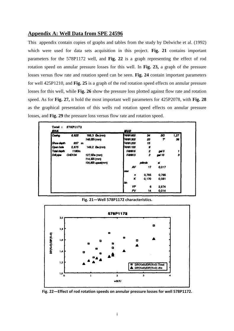
i
Appendix A: Well Data from SPE 24596 This appendix contain copies of graphs and tables from the study by Delwiche et al. (1992)
which were used for data sets acquisition in this project. Fig. 21 contains important
parameters for the 578P1172 well, and Fig. 22 is a graph representing the effect of rod
rotation speed on annular pressure losses for this well. In Fig. 23, a graph of the pressure
losses versus flow rate and rotation speed can be seen. Fig. 24 contain important parameters
for well 425P1210, and Fig. 25 is a graph of the rod rotation speed effects on annular pressure
losses for this well, while Fig. 26 show the pressure loss plotted against flow rate and rotation
speed. As for Fig. 27, it hold the most important well parameters for 425P2078, with Fig. 28
as the graphical presentation of this wells rod rotation speed effects on annular pressure
losses, and Fig. 29 the pressure loss versus flow rate and rotation speed.
Fig. 21—Well 578P1172 characteristics.
Fig. 22—Effect of rod rotation speeds on annular pressure losses for well 578P1172.

ii
Fig. 23—Total pressure losses in function of mud flow rates and rotation speed for well 578P1172
Fig. 24—Well 425P1210 characteristics.
Fig. 25—Effect of rod rotation speeds on annular pressure losses for well 425P1210.
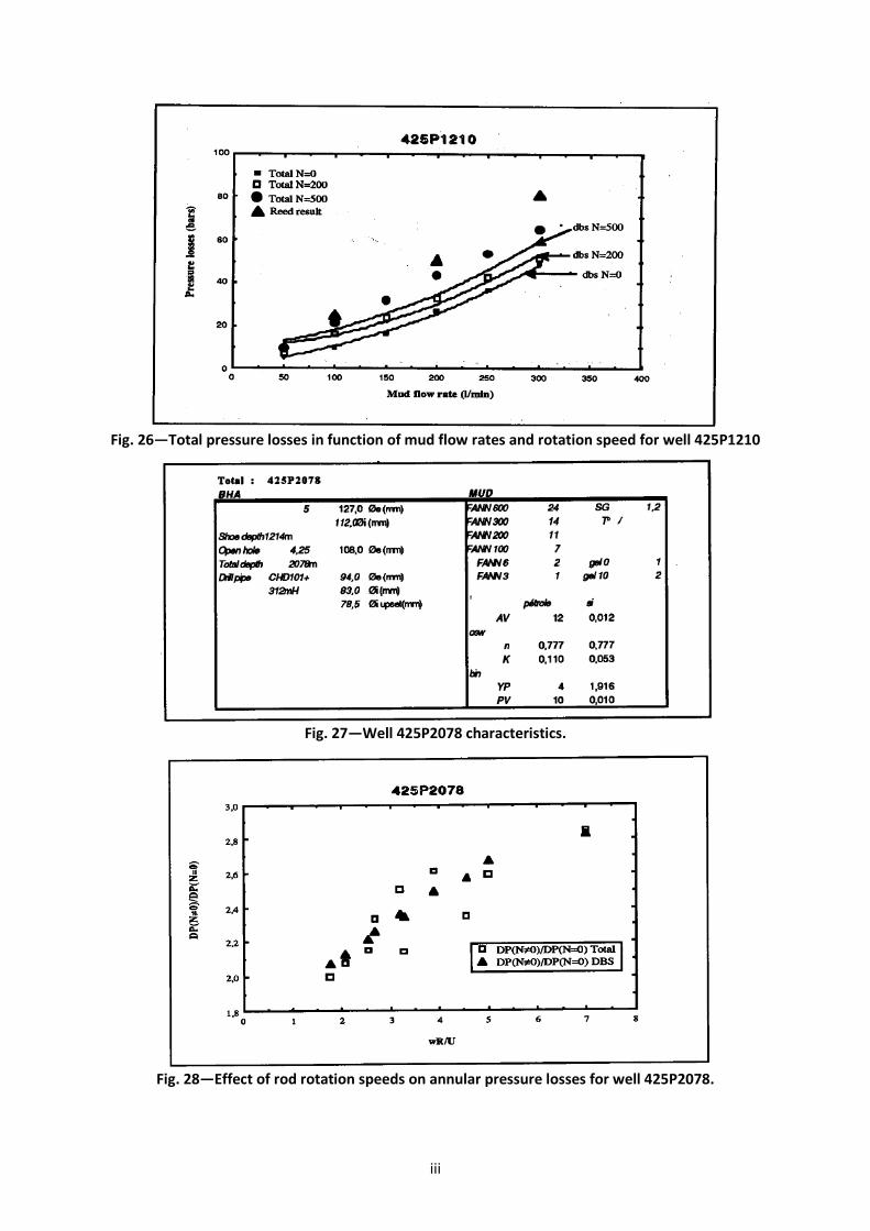
iii
Fig. 26—Total pressure losses in function of mud flow rates and rotation speed for well 425P1210
Fig. 27—Well 425P2078 characteristics.
Fig. 28—Effect of rod rotation speeds on annular pressure losses for well 425P2078.
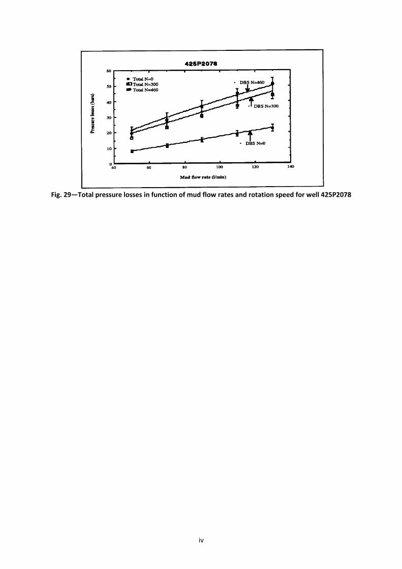
iv
Fig. 29—Total pressure losses in function of mud flow rates and rotation speed for well 425P2078

v
Appendix B: Well Data from SPE 59265 This appendix contain copies of the graphs and tables from the study of Haige et al. (2000)
which were used for data sets acquisition in this project. Fig. 30 shows the graph of drillpipe
rotational effects on annular pressure losses for three fluid velocities that was presented in this
study of well Miao 1-40.
Fig. 30—Effects of drillpipe rotation speed on annular pressure losses in the Miao 1-40 well.

vi

vii
Appendix C: Well Data from SPE 87149 This appendix contain copies of the graphs and tables from the study by Diaz et al. (2004)
which were used for data sets acquisition in this project. Fig. 31 contains properties used in
calculation with water as the drilling fluid, while Fig. 32 contains the same information for
the two other drilling fluids, Mud A and Mud B.
Fig. 31—Fluid and cuttings properties with water as drilling fluid
Fig. 32—Fluid properties for Mud A and Mud B drilling fluids
The measured and calculated data was in this study presented for three different flow rates,
and for each of these flow rates measurements were done with the three various drilling
fluids, water, Mud A and Mud B. In Fig. 33, a graph showing BHP versus rotary speed with
water as drilling fluid is presented. The hole diameter was 12.715 in., the outer casing
diameter was 11.75 in., the true depth was 86.26 m, and the flow rate was 0.022 m3/s. Fig. 34
show the same graph, but with a new flow rate of 0.028 m3/s. In Fig. 35, the graph is shown
for a flow rate of 0.035 m3/s. In Fig. 36, the graph is showing BHP versus rotary speed with
Mud A as drilling fluid. Again, the hole diameter was 12.715 in., the outer casing diameter
was 11.75 in., and the true depth was 86.26 m. In this figure, the flow rate was 0.022 m3/s.
Fig. 37 show the same graph with a flow rate of 0.028 m3/s, and Fig. 38 show the graph for
the situation of a 0.035 m3/s flow rate. Fig. 39 contains a graph of the BHP versus rotary
speed with a flow rate of 0.022 m3/s, and with Mud B as the drilling fluid. Here as well the
hole diameter is 12.715 in., the casing OD is 11.75 in., and the depth is at 86.26 m. Fig. 40
and Fig. 41 show the same graph, but with a flow rate of 0.028 m3/s and 0.035 m3/s
respectively.

viii
Fig. 33—Bottomhole pressure versus rotary speed. Drilling fluid is water. Dh=12.715 in., OD=11.75 in., TD=85.26 m, Q=0.022 m3/s.
Fig. 34—Bottomhole pressure versus rotary speed. Drilling fluid is water. Dh=12.715 in., OD=11.75 in., TD=86.26 m, Q=0.028 m3/s.
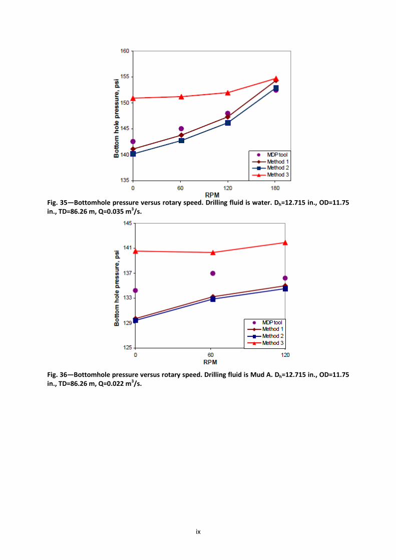
ix
Fig. 35—Bottomhole pressure versus rotary speed. Drilling fluid is water. Dh=12.715 in., OD=11.75 in., TD=86.26 m, Q=0.035 m3/s.
Fig. 36—Bottomhole pressure versus rotary speed. Drilling fluid is Mud A. Dh=12.715 in., OD=11.75 in., TD=86.26 m, Q=0.022 m3/s.

x
Fig. 37—Bottomhole pressure versus rotary speed. Drilling fluid is Mud A. Dh=12.715 in., OD=11.75 in., TD=86.26 m, Q=0.028 m3/s.
Fig. 38—Bottomhole pressure versus rotary speed. Drilling fluid is Mud A. Dh=12.715 in., OD=11.75 in., TD=86.26 m, Q=0.035 m3/s.

xi
Fig. 39—Bottomhole pressure versus rotary speed. Drilling fluid is Mud B. Dh=12.715 in., OD=11.75 in., TD=86.26 m, Q=0.022 m3/s.
Fig. 40—Bottomhole pressure versus rotary speed. Drilling fluid is Mud B. Dh=12.715 in., OD=11.75 in., TD=86.26 m, Q=0.028 m3/s.

xii
Fig. 41—Bottomhole pressure versus rotary speed. Drilling fluid is Mud B. Dh=12.715 in., OD=11.75 in., TD=86.26 m, Q=0.035 m3/s.

xiii
Appendix D: Well Data from SPE 19526 This appendix contain a copy of the drilling data from Bode et al. (1989), used in the
development of empirical equations. Fig. 42 contain a graph presented in this study, showing
the Reynolds number plotted against the annular pressure losses with rotation over that of no
rotation, for three different rotation speeds.
Fig. 42—Annular pressure losses with rotation over annular pressure losses without rotation plotted against the Reynolds number for three rotation speeds.

xiv

xv
Appendix E: Well Data from SPE 110470 This appendix contains a copy of 22/30c-G4 well data from Hemphill et al. (2007). The data
is presented in Fig. 43, and show the data on the form Measured Change in ECD vs. Drillpipe
Rotation Speed. Two data sets were gathered from this figure, called Elf 8.75-in A and Elf
8.75-in B.
Fig. 43—Measured Change in ECD plotted against RPM for ELF 8.75-in A and ELF 8.75-in B

xvi

xvii
Appendix F: Well Data from SPE 26343 This appendix contains a copy of the graph representing the data sets from the SHDT.1 well
in McCann et al. (1993). The graph is presented in Fig. 44, and show the annular pressure vs.
flow rate for rotation rates of 300 and 600 RPM.
Fig. 44—Annular pressure plotted against flow rate. RPM is 300 and 600

xviii

xix
Appendix G: Input Values for Calculations with PLR-Equation This appendix contains a summary of the input values used when doing calculations with the
PLR-equation. Table 24 contain input values for the 1300 kg/m3 mud, Table 25 contain input
values for the 1500 kg/m3 mud, and Table 26 contain input values for the 1700 kg/m3 mud. In
Fig. 45, the resulting log-log plot from the Herschel-Bulkley 3 point oil field approach for
calculation of n is shown for the 1300 kg/m3 mud, and in Fig. 46 and Fig. 47, the same plot is
shown for the 1500 kg/m3 and 1700 kg/m3 mud respectively.
Table 24—Input values in PLR-calculations. Mud weight is 1300 kg/m3, rotations speed 120 RPM to the left, 60 RPM to the right
Parameter Value Units
Parameter Value Units ρ 1300 kg/m3
ρ 1300 kg/m3
τy 8.6184 Pa
τy 8.6184 Pa U 1.9735 m/s
U 1.9735 m/s
εave 0.5
εave 0.5 n 0.3449
n 0.3449
Ta 175 000
Ta 43 700 Reeff 755
Reeff 755
k 0.7647
k 0.7647 Dp 0.1651 m
Dp 0.1651 m
Dh 0.2159 m
Dh 0.2159 m ω 120 RPM
ω 60 RPM
μapp 0.0470 Pa∙s
μapp 0.0470 Pa∙s MD 2000 m
MD 2000 m
Li xxxx m
Li xxxx m Ei xxxx
Ei xxxx
DTJ 0.1651 m
DTJ 0.1651 m τw,lam 53.6259 Pa
τw,lam 53.6259 Pa
Fig. 45—Log-log plot from Herschel-Bulkley 3 point oil field approach calculation of n by use of 1300 kg/m3 mud
y = 4,9134x0,3449
1
10
100
1 10 100 1000 10000

xx
Table 25—Input values in PLR-calculations. Mud weight is 1500 kg/m3, rotation speed 120 RPM to the left, 60 RPM to the right
Parameter Value Units
Parameter Value Units ρ 1500 kg/m3
ρ 1500 kg/m3
τy 11.4913 Pa
τy 11.4913 Pa U 1.9735 m/s
U 1.9735 m/s
εave 0.5
εave 0.5 n 0.3432
n 0.3432
Ta 133 000
Ta 33 200 Reeff 660
Reeff 660
k 0.7647
k 0.7647 Dp 0.1651 m
Dp 0.1651 m
Dh 0.2159 m
Dh 0.2159 m ω 120 RPM
ω 60 RPM
μapp 0.0620 Pa∙s
μapp 0.0620 Pa∙s MD 2000 m
MD 2000 m
Li xxxx m
Li xxxx m Ei xxxx
Ei xxxx
DTJ 0.1651 m
DTJ 0.1651 m τw,lam 70.8628 Pa
τw,lam 70.8628 Pa
Fig. 46—Log-log plot from Herschel-Bulkley 3 point oil field approach calculation of n by use of 1500 kg/m3 mud
y = 6,5693x0,3432
1
10
100
1 10 100 1000 10000

xxi
Table 26—Input values in PLR-calculations. Mud weight is 1700 kg/m3, rotation speed 120 RPM to the left, 60 RPM to the right
Parameter Value Units
Parameter Value Units ρ 1700 kg/m3
ρ 1700 kg/m3
τy 15.3217 Pa
τy 15.3217 Pa U 1.9735 m/s
U 1.9735 m/s
εave 0.5
εave 0.5 n 0.3458
n 0.3458
Ta 60 200
Ta 22 500 Reeff 553
Reeff 553
k 0.7647
k 0.7647 Dp 0.1651 m
Dp 0.1651 m
Dh 0.2159 m
Dh 0.2159 m ω 120 RPM
ω 60 RPM
μapp 0.0840 Pa∙s
μapp 0.0840 Pa∙s MD 2000 m
MD 2000 m
Li xxxx m
Li xxxx m Ei xxxx
Ei xxxx
DTJ 0.1651 m
DTJ 0.1651 m τw,lam 95.7605 Pa
τw,lam 95.7605 Pa
Fig. 47—Log-log plot from Herschel-Bulkley 3 point oil field approach calculation of n by use of 1700 kg/m3 mud
y = 8,7229x0,3458
1
10
100
1 10 100 1000 10000

xxii
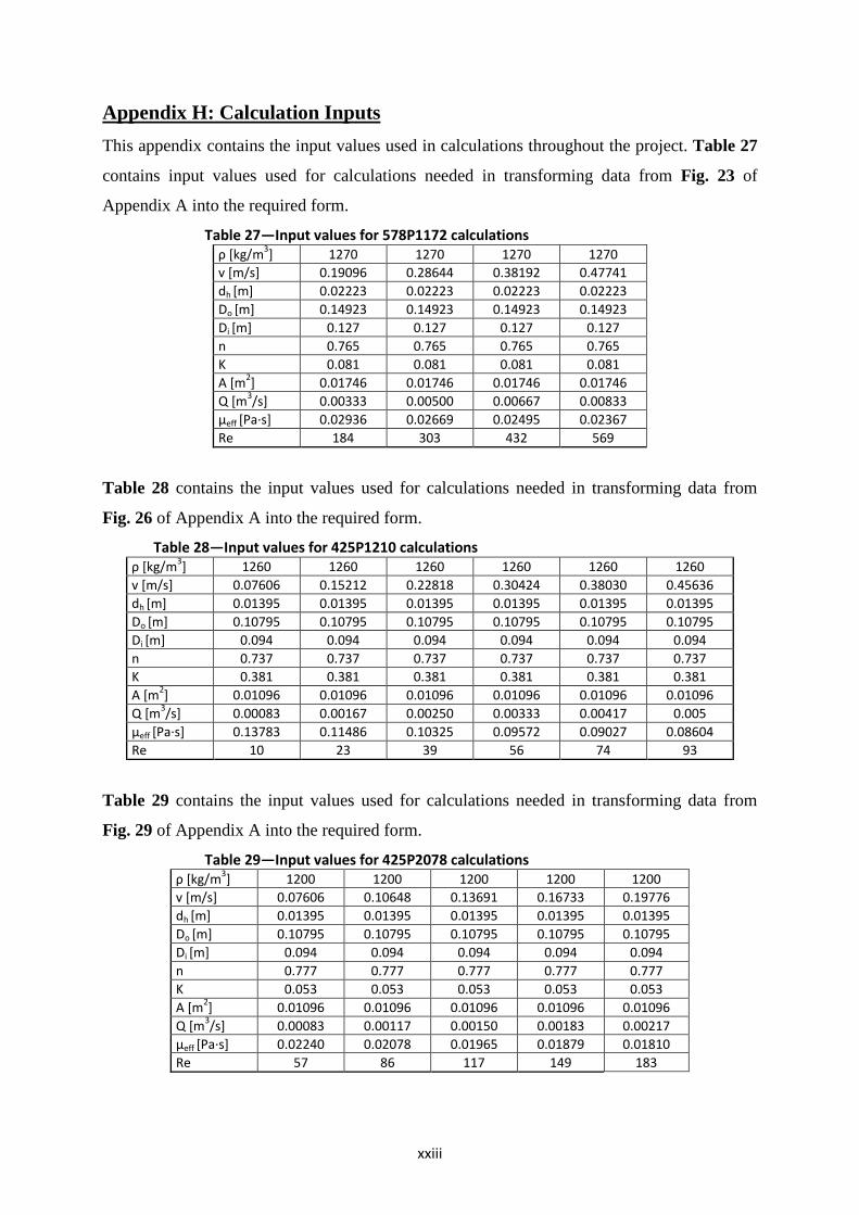
xxiii
Appendix H: Calculation Inputs This appendix contains the input values used in calculations throughout the project. Table 27
contains input values used for calculations needed in transforming data from Fig. 23 of
Appendix A into the required form.
Table 27—Input values for 578P1172 calculations ρ [kg/m3] 1270 1270 1270 1270 v [m/s] 0.19096 0.28644 0.38192 0.47741 dh [m] 0.02223 0.02223 0.02223 0.02223 Do [m] 0.14923 0.14923 0.14923 0.14923 Di [m] 0.127 0.127 0.127 0.127 n 0.765 0.765 0.765 0.765 K 0.081 0.081 0.081 0.081 A [m2] 0.01746 0.01746 0.01746 0.01746 Q [m3/s] 0.00333 0.00500 0.00667 0.00833 μeff [Pa∙s] 0.02936 0.02669 0.02495 0.02367 Re 184 303 432 569
Table 28 contains the input values used for calculations needed in transforming data from
Fig. 26 of Appendix A into the required form.
Table 28—Input values for 425P1210 calculations ρ [kg/m3] 1260 1260 1260 1260 1260 1260 v [m/s] 0.07606 0.15212 0.22818 0.30424 0.38030 0.45636 dh [m] 0.01395 0.01395 0.01395 0.01395 0.01395 0.01395 Do [m] 0.10795 0.10795 0.10795 0.10795 0.10795 0.10795 Di [m] 0.094 0.094 0.094 0.094 0.094 0.094 n 0.737 0.737 0.737 0.737 0.737 0.737 K 0.381 0.381 0.381 0.381 0.381 0.381 A [m2] 0.01096 0.01096 0.01096 0.01096 0.01096 0.01096 Q [m3/s] 0.00083 0.00167 0.00250 0.00333 0.00417 0.005 μeff [Pa∙s] 0.13783 0.11486 0.10325 0.09572 0.09027 0.08604 Re 10 23 39 56 74 93
Table 29 contains the input values used for calculations needed in transforming data from
Fig. 29 of Appendix A into the required form.
Table 29—Input values for 425P2078 calculations ρ [kg/m3] 1200 1200 1200 1200 1200 v [m/s] 0.07606 0.10648 0.13691 0.16733 0.19776 dh [m] 0.01395 0.01395 0.01395 0.01395 0.01395 Do [m] 0.10795 0.10795 0.10795 0.10795 0.10795 Di [m] 0.094 0.094 0.094 0.094 0.094 n 0.777 0.777 0.777 0.777 0.777 K 0.053 0.053 0.053 0.053 0.053 A [m2] 0.01096 0.01096 0.01096 0.01096 0.01096 Q [m3/s] 0.00083 0.00117 0.00150 0.00183 0.00217 μeff [Pa∙s] 0.02240 0.02078 0.01965 0.01879 0.01810 Re 57 86 117 149 183

xxiv
In Table 30, the input values for calculations performed on the data read from Fig. 44 of
Appendix F is seen.
Table 30—Input values for SHDT.1 calculations ρ [kg/m3] 1000 1000 1000 1000 1000 1000 1000 1000 1000 1000 1000 v [m/s] 0.652 0.869 1.086 1.303 1.52 1.737 1.955 2.172 2.389 2.606 2.823 dh [m] 0.018 0.018 0.018 0.018 0.018 0.018 0.018 0.018 0.018 0.018 0.018 Do [m] 0.112 0.112 0.112 0.112 0.112 0.112 0.112 0.112 0.112 0.112 0.112 Di [m] 0.094 0.094 0.094 0.094 0.094 0.094 0.094 0.094 0.094 0.094 0.094 τ300 [Pa] 20 20 20 20 20 20 20 20 20 20 20 γ300 [s
-1] 511 511 511 511 511 511 511 511 511 511 511 A [m2] 0.0029 0.0029 0.0029 0.0029 0.0029 0.0029 0.0029 0.0029 0.0029 0.0029 0.0029 Q [m3/s] 0.0019 0.0025 0.0032 0.0038 0.0044 0.005 0.0057 0.0063 0.0069 0.0076 0.0082 μeff [Pa∙s] 0.0391 0.0391 0.0391 0.0391 0.0391 0.0391 0.0391 0.0391 0.0391 0.0391 0.0391 Re 298 398 497 597 696 796 895 995 1094 1194 1293

xxv
Unit Conversion Factors Below is a table with conversion factors from oil field units to SI metric units (Table 31), and
a table with conversion factors from other units to SI metric units (Table 32).
Table 31—Conversion factors from oil field units to SI units
Oil Field Units Conversion Factor SI Metric Unit ft 3.048000 E−01 m in 2.540000 E−02 m lbm/gal (PPG) 1.198264 E+02 kg/m3 ft2 9.290304 E−02 m2 lb/ft 1.488189 E+00 kg/m cP 1.000000 E−03 Pa∙s psi 6.894760 E+03 Pa ft/min 5.080000 E−03 m/s gal/min (GPM) 6.309020 E−05 m3/s psi/ft 2.262060 E+04 Pa/m
Table 32—Conversion factors from other units SI units
Other Units Conversion Factor SI Metric Unit LPM 6.000000 E−04 m3/s cm 1.000000 E−02 m SG 1.000000 E+03 kg/m3 °C °C + 273.15 °K bar 1.000000 E+04 Pa mm 1.000000 E−03 m