Does Volatility Improve UK Earnings Forecasts&quest

Does Volatility Improve UK Earnings Forecasts?

Nikola Petrovic, Stuart Manson∗ and Jerry Coakley Department of Accounting, Finance and Management, University of Essex

Abstract: We investigate the relation between UK accounting earnings volatility and the level of future earnings in a risk management framework. Our unique sample comprises some 11,107 firm-year observations for 1,548 non-financial firms over the 1980-2003 period. The findings confirm the established in-sample result of an inverse volatility-earnings relation. This is more pronounced as the current level of earnings and the firm's growth opportunities increase. However, we find that earnings are mainly explained by lagged earnings and there is no improvement in out-of-sample forecast accuracy when volatility is added as a regressor. Keywords: Earnings volatility, earnings predictability, risk management theory

∗ Corresponding author. Tel: +44 (0)1206872063. Fax: +44 (0)1206 873429. Email: [email protected]

1. INTRODUCTION

The importance of earnings volatility for a firm’s value has long been recognized in the

accounting and finance literature. Such volatility can have an impact either through its relation to

the discount rate or expected cash flows (earnings) in valuation models. Most existing research

has focused on the link to the discount rate or cost of capital. One established result is a positive

relationship between earnings volatility and different measures of the cost of capital. For

example, Beaver, Kettler and Scholes (1970) provide evidence that the variance of the earnings-

to-price ratio is the accounting variable that is most correlated with a firm’s beta coefficient.

Minton and Schrand (1999) find that historical earnings volatility is strongly associated with the

beta coefficient, dividend payout ratio and share price volatility. Gebhardt, Lee and Swaminatham

(2001) show that earnings volatility - measured as the standard deviation of earnings per share - is

strongly associated with the ex ante cost of capital implied from the residual income model.

A few recent studies directly test the link between the value of a firm and earnings volatility

for the US market. Barnes (2001) find that earnings volatility is negatively related to firm value

measured by the market-to-book ratio. Allayannis et al. (2005) show the same relation holds but

only before controlling for cash flow volatility. However, there is virtually no research on the

relation between current earnings volatility and future performance. This matters since the

documented increased risk effect of such volatility may be affected through its effect on the level

of future earnings in the numerator of the valuation formula.

Risk management theories propose several explanations for why a reduction in earnings

volatility can increase the value of the firm through higher expected earnings.1 Firstly, the

probability of financial distress and its expected direct and indirect costs increase with earnings

volatility. Distressed firms also have a higher propensity for undertaking negative and foregoing

positive net present value projects due to agency problems. Secondly, higher earnings volatility

1 For an excellent review, see Bartram (2000).

1

tends to reduce the supply of internal funds to finance investment opportunities and so increases

the likelihood of facing more expensive external funds, resulting in foregone investment. Finally,

the more volatile earnings are, the higher is expected expense for corporate taxes (see e.g. Smith

and Stulz, 1985; Bartram, 2000; Graham and Rogers, 2002). Relatedly, the compensation of risk-

averse and undiversified managers, whose expected utility is concave in compensation, increases

with earnings volatility as a reward for bearing non-diversifiable risk (Smith and Stulz, 1985).

Motivated by the underinvestment effect on expected cash flows, Minton, Schrand and

Walther (2002) (hereinafter MSW) were the first to explore the impact of volatility on future

earnings. They show for a US sample of 3,501 non-financial firm-year observations in the 1987-

1999 period, that current cash flow (earnings) volatility is negatively related to future cash flow

(earnings) in terms of lower forecast error and less biased predictions.2 They provide some

evidence that investors do not fully understand the implications of current performance volatility

for future performance levels. A trading strategy involving buying (selling) the stocks where the

earnings’ (cash flow) forecast from a model that includes volatility is higher (lower) from one that

excludes it earns small but significant excess size-adjusted return of 3-5%.

This paper makes several contributions. First, given the paucity of studies on the relation

between current earnings volatility and future earnings, this paper seeks to fill the lacuna in the

literature. It does so using a sample of 11,107 UK firm-year observations for 1,548 non-financial

firms over the 1985-2003 sample period.3 As such, it is the first large scale non-US study on the

importance of earnings volatility for forecasting future earnings. The observed negative relation

in the UK is consistent with the corresponding MSW finding for the US. However, our

2 Volatility is measured by the coefficient of variation. 3 Although we could have used the same risk management framework if we had tested for the relation between current and future cash flows, we focus only on earnings. There is a large accounting literature showing that earnings are a better measure of true firm performance than operating cash flows. See for example Dechow (1994), Dechow, Kothari and Watts (1998), and Ball and Shivakumar (2006). Only a few studies such as Lev et al. (2005) dispute this. Moreover, forecasting earnings is a starting point in any valuation exercise regardless of the model used. Financial analysts prefer to forecast earnings rather than cash flows and rely more on earnings based than on cash flow based valuation models (Demirakos, Strong and Walker, 2004).

2

results on the statistical significance of earnings volatility depend on the specification

used and so are only partially consistent with MSW. Second, the adverse value impact

associated with earnings volatility can be expected to vary across firms due to their differential

sensitivity to the costs of market imperfections. Therefore, we develop and test novel hypotheses

for cross-sectional differences in the volatility-future earnings relation using firm characteristics

such as growth, leverage, size and liquidity. The latter capture costs related not only to the risk of

underinvestment due to higher costs of external capital but also costs related to companies’

exposure to the likelihood of bankruptcy and agency costs of debt related underinvestment.4

Finally, the empirical results for our UK sample cast doubt on existing US findings that

including earnings volatility as a regressor improves the accuracy of forecasting future earnings.

First, while earnings volatility is a statistically significant predictor of future earnings over and

above the current earnings, this is mainly as a second-order effect. It impacts through its

interaction with the level of current earnings by decreasing their persistence coefficient rather

than through a separate link. Second, our cross-section association test indicates that earnings

volatility has a negative relationship with future earnings mainly through the under-investment

effect and not through financial distress. This negative relation is more pronounced as the market-

to-book ratio increases (under-investment effect), whereas, in general, it is not sensitive to

differences in financial leverage (financial distress) as well as to differences in liquidity and firm

size. Finally, we find that the use of earnings volatility as an additional regressor does not help in

forecasting earnings levels. The explanatory power, forecast accuracy and forecast bias of the

earnings prediction model containing earnings volatility is not statistically different from a

benchmark model which includes only lagged earnings as an explanatory variable.

The paper proceeds as follows. The main hypotheses are outlined in Section 2. Section 3

describes the sample, defines the variables and provides some summary statistics. Section 4 4 This is consistent with Nissim (2002) who argues that the MSW finding of a negative relation between earnings/cash flow volatility and subsequent earnings/cash flow levels cannot be explained solely by the underinvestment effect.

3

describes the empirical methods used and analyses the main findings and in Section 5 some

conclusions are provided.

2. HYPOTHESIS DEVELOPMENT

(i) Relation between earnings volatility and future earnings

Good estimates of future earnings are a prerequisite for accurate equity valuation. One of the key

findings of corporate risk management literature is that cash flow volatility causes deadweight

costs that reduce expected cash flow in the numerator of the valuation formula. This proposed

negative link between volatility and expected cash flows can be used to improve earnings

forecasts, by using earnings volatility as a proxy for cash flow volatility and future earnings as

proxy for expected cash flows. 5 The economic intuition behind this idea is explained below.

Costs of financial distress. Higher cash flow volatility increases the probability of lower

realizations of future cash flows and consequently the probability of financial distress increases

especially when there is a large debt exposure. Financial distress causes indirect costs for

companies to the extent that suppliers, customers and employees react by requiring favourable

contracts relative to non-distressed firms. This results in lower expected revenues and higher

expenses for such firms (see e.g. Bartram, 2000; Smith and Stulz, 1985).

Agency costs of debt (underinvestment and asset substitution). Financially distressed firms

are tempted to forego positive NPV projects if their benefits go to the debtholders. Similarly, due

to the option nature of equity, they may undertake risky negative NPV projects which increase the

value of equity at the expense of debtholders. On average, the foregone investment and negative

NPV projects reduce expected earnings. The likelihood of distress and consequently the effect of

these agency costs increases in earnings volatility (see e.g. Bartram, 2000; Stulz, 2003).

5 Corporate risk management literature has developed in order to justify the use of derivatives for the purpose of reduction in corporate value volatility. Subsequently, many empirical studies tested whether the use of derivatives can be justified by the firm-specific sensitivity to market imperfection costs. To our knowledge, only MSW’s study use this intuition in the earnings’ forecasting context.

4

Costs of accessing external capital. Due to information asymmetry between managers and

capital markets, external financing of new investments is more costly than internal financing.

Therefore, firms often forego profitable investment opportunities when faced with a lack of

internal funds. Lower investment, in turn, leads to lower future expected earnings. Since earnings

volatility increases the likelihood of insufficient internal funds, the former is negatively related to

expected earnings (see e.g. Bartram, 2000; Froot, Scharfstein, and Stein, 1993; MSW).

Management incentives. Undiversified and risk averse managers require higher compensation

for non-diversifiable risk since expected utility is concave in compensation. Higher expected

compensation lowers future earnings. This is also true for other undiversified claimholders such

as employees or, in the case of imperfect market structures, suppliers and customers. The impact

of risk reduction on expected management compensation depends on the design on the manager’s

compensation contract. If it is concave in the firm value, then risk reduction will increase their

compensation thus offsetting the risk-aversion effect. In the case of a convex function such as

management stock options, the negative effect of the risk on compensation is more pronounced

(see e.g. Smith and Stulz, 1985; Bartram, 2000).

Taxes. Marginal tax rates which move in line with increases in taxable income, and delayed

tax benefits from carry forward and carry backward tax rules make the present value of expected

income tax increasing in the volatility of pre-tax earnings. Consequently, expected post-tax

earnings are lower for those firms with higher earnings volatility (see e.g. Smith and Stulz, 1985;

Bartram, 2000; Graham and Rogers, 2002).

These explanations lead to our first directional hypothesis:6

H1: Future earnings are negatively related to current earnings volatility.

Our empirical tests focus on reported volatility. Reported earnings are assumed to be ‘smoothed’

after a mix of optimal actions (such as usage of derivatives and diversification) is undertaken to

6 We acknowledge that the opposite hypothesis that the earnings volatility is positively related to future earnings may also hold to the extent that managers modify or abandon loss-making projects and so make negative cash flows less permanent than positive ones (Berger, Ofek and Swary, 1996).

5

minimize the total costs of volatility.7 Total costs are given as a sum of costs of risk reducing

actions and costs of bearing remaining risk, and are minimized to the point where the marginal

costs of further volatility reduction are equal to the marginal costs of bearing remaining volatility

(Shin and Stulz, 2000).8 Since there always exists some volatility with its associated costs, the

proposed inverse relation holds both for reported and non-observable pre-smoothed earnings.

(ii) Cross-sectional variation

While the impact of the earnings volatility on future earnings is hypothesized to be negative due

to market imperfections, the associated costs vary with firm-specific characteristics.

Consequently, this negative incremental impact of earnings volatility on future earnings will be

more pronounced as these costs increase. We follow the empirical risk management and corporate

finance literature to capture these firm specific characteristics (e.g. Nance and Smith, 1993;

Bartram, 2000; Graham and Rogers, 2002).

The agency costs of debt and associated underinvestment are related to a firm’s growth

options. The implication is that firms with higher volatility and agency costs of debt invest less

(since the benefits accrue to debtholders) or they undertake more negative NPV projects. Thus,

for a given level of earnings volatility, an increase in growth opportunities has a negative impact

on future earnings since less is invested than full capacity allows. This does not mean that firms

with higher growth prospects have lower earnings than firms with lower prospects. Instead, the

foregone increase in earnings is lower than it could have been if the opportunities had been fully

exploited.

7 Derivatives (neither at their cost or fair value) were not required to be reported in the balance sheet and profit and loss account until the recent adoption of IAS 39. Also, most of the assets in the sample period are reported at historical cost. Therefore, the impact of derivatives on the reduction in the variability of reported earnings is negligible. 8 While residual volatility is costly, the alternatives actions may be even more expensive. For example, small firms can find the use of derivatives more expensive due to direct transaction costs and the fixed costs of information services, expertise and know-how when contrasted with the opportunity costs of the volatility.

6

The same line of reasoning holds for the external costs of financing. Firms with insufficient

funds opt not to invest if they cannot earn the hurdle rate of return needed to borrow. The

foregone increase in earnings due to earnings volatility is higher for firms with better growth

prospects. This intuition can be summarized in the following hypothesis:

H2a: The negative impact of the earnings volatility on future earnings increases with growth

opportunities.

The underinvestment problem matters less for firms with internal funds. If the firm has high

levels of cash and liquidity, the adverse impact of earnings volatility on investment and future

earnings is likely to be less pronounced (MSW, 2002). Investment in liquid assets reduces the

overall risk of a company’s assets and the resulting likelihood of default (Nance, Smith and

Smithson, 1993) which also counterbalances the volatility effect on future earnings. This leads to

the following hypothesis:

H2b: The negative impact of the earnings volatility on future earnings decreases with the

liquidity of the firm.

The probability of distress is negatively related to a firm’s debt exposure and therefore if a firm

carries relatively little debt, earnings volatility may not be relevant since firms do not go bankrupt

even with low earnings realizations. Consequently, high earnings volatility combined with low

financial leverage does not impose significant indirect expected costs of distress and vice versa.

For a given level of volatility, a higher level of financial leverage is negatively related with future

earnings which leads to the following hypothesis:

H2c: The negative impact of earnings volatility on future earnings increases with financial

leverage.

High leverage also increases the agency costs of debt. However, the non-linear relation between

earnings volatility and the magnitude of those costs depends on the available growth options,

which is captured by H2a.

7

There is some empirical evidence that the magnitude of the costs of bankruptcy is negatively

related to a firm’s size and hence they are relatively more important for small rather than large

firms (Warner, 1977). As a result, earnings volatility is less costly as firm size increases. For a

given level of volatility, an increase in the firm size reduces its negative impact on future

earnings.

H2d: The negative impact of earnings volatility on future earnings decreases with the size of

the firm.9

3. SAMPLE DESCRIPTION AND VARIABLE MEASUREMENT

(i) Data

The sample consists of non-financial firms listed on the London Stock Exchange from 1980 to

2003. The dataset consists of 11,107 firm-year observations (1,548 distinct non-financial firms)

for those firms with sufficient data to calculate operating earnings and earnings volatility. We

divide the sample into 19 five-year overlapping periods (1981-1985 is the first and 1999-2003 is

the last). The number of observations per period is in the range from 214 in 1987 to 878 in 1996.

All the variables were extracted from Datastream Worldscope database.

(ii) Earnings and earnings volatility

Annual earnings are defined as operating profit after exclusion of the items of an exceptional

nature, which do not form part of a company’s normal trading activities, but before

depreciation (Datastream Worldscope item WC01250 plus WC01151). The earnings measure is

scaled by average total assets (Worldscope Datastream item WC02999) which is consistent with

other similar studies.

9 Whilst we would like to test for hypotheses related to taxation and management incentives, we are unable to collect relevant data for such purposes.

8

Current earnings volatility (EV) is measured as the coefficient of variation over the first four

years in the five-year period. Unlike most existing studies, we do not use interim (the half-year or

quarterly) data but annual data for the volatility calculation since the former are subject to the

criticism of ignoring seasonal effects (Nissim, 2002). The coefficient of variation is widely used

in the related literature (e.g. MSW; Michelson et al., 1995) and is calculated as the standard

deviation of the unscaled earnings series divided by the mean of the absolute values. We use the

mean of the absolute values in the denominator rather than the mean of the actual values to

control for size by focusing on the magnitude of earnings irrespective of their sign. The earnings

and earnings volatility variables are winsorized at the 1st and 99th percent level to reduce the effect

of extreme observations.

(iii) Firm specific characteristics

We use several different variables to test H2 that the negative impact of the earnings volatility is

more pronounced for firms with better investment opportunities and are less liquid, highly

leveraged, and smaller (Nance and Smithson, 1993; Graham and Rogers, 2002; Bartram, 2000).

Growth opportunities are measured by the market-to-book value of the firm (MTB).10,11

Leverage (DTC) is measured as total debt-to-capital ratio expressed in percentage points. Size is

measured as the average of the natural logarithm of total assets (lnTA) and liquidity by the

current ratio (CR). MTB, DTC, lnTA and CR are calculated as an average value over the first

four years in the five-year period. We also use current year cash and cash equivalents scaled by

average total assets (CEt) to capture the influence of cash levels on the under-investment effect.

CR is winsorized at the 1% and 99% level to control for outliers, while MTB, and CEt are

winsorized at the 99% level (they are bounded below at zero). 10 Detailed definitions of firm-specific characteristics are provided in Appendix 1. 11 Alternatively, we used capital expenditure (WC04601) defined as the cash paid for the purchase of fixed assets scaled by average total assets. The results for this growth variable are mixed perhaps because capital expenditure is an indicator of actual growth rates and not necessarily growth opportunities. Results are available from the authors on request.

9

(iv) Summary statistics

Table 1 present summary statistics of the variables used in subsequent tests.

[Table 1 around here]

The future, one-year ahead mean (median) earnings level of 0.126 (0.129) is in line with the

current mean (median) earnings level of 0.130 (0.132). The sample is moderately left skewed in

the earnings variable. Descriptive statistics show large variation in firm-specific volatility. The

standard deviation of the coefficient of variation of 0.319 is in line with its mean value of 0.369.

Both volatility measures are right-skewed which is expected since they are bounded below at

zero. This is also the case for the control variables.

The correlation between the variables is presented in Table 2.


The correlation signs are generally supportive of our hypotheses. Earnings volatility is

significantly negatively correlated with future earnings with a coefficient of -0.34. Most of the

control variables exhibit a relatively low correlation with future earnings. The exception is CR

(-0.24). Liquidity is positively correlated with lower profitability perhaps due to investment in

more liquid and consequently less profitable assets. The size variable (lnTA) is significantly

negatively related to the earnings volatility (around -0.37).

4. EMPIRICAL RESULTS

(i) Predictive ability of earnings volatility

The starting point in forecasting future one-year ahead earnings is current earnings. Therefore, it

is valuable to explore whether the negative relation between earnings volatility and future

earnings is still valid after controlling for current earnings (H1). We use several regression tests

for this.

10

Firstly, our benchmark model (Model 1) regresses future earnings on current earnings.

Second, Model 2 includes earnings volatility as an extra regressor. Third, Model 3 regresses

future earnings on current earnings and an interaction term of current earnings multiplied by

earnings volatility. The latter term is added because there is some evidence that earnings volatility

affects not only the future earnings level but also earnings persistence. Dichev and Tang (2005)

show for an US sample that the earnings persistence coefficient from a pooled regression of

earnings one-year ahead on current earnings is inversely related to earnings volatility.12 Finally,

we estimate the regression with current earnings, earnings volatility and an interaction term as

independent variables (Model 4).

The annual cross-section rolling regressions are estimated for 19 five-year sample periods. In

this way, the number of holdout sample periods to examine forecast accuracy of different

specifications is maximized. In addition, Fama and French (2000) argue that this procedure is

superior to pooled OLS estimators because the variation of the annual slopes allows for cross-

sectional correlation of residuals across the firms.

We examine the economic significance of those estimates for equity valuation by testing the

forecast accuracy of our four models and checking for systematic over- or under-prediction of

next year’s earnings (forecast bias). The coefficients estimated in year t are used to forecast

earnings in year t+1. Forecasting is performed on the total sample available for year t+1 no

matter whether the firms included are used for coefficient estimation purposes in year t.

Several measures of forecast accuracy are calculated. Absolute error (AE) is calculated as the

absolute value of the difference between actual and predicted earnings whilst bias proportion is

calculated as the difference between actual and predicted earnings. For consistency with

comparable studies such as MSW we calculate relative measures of accuracy as well. The

absolute percentage error (APE) is calculated as the absolute value of the difference between

actual and forecasted earnings divided by absolute actual earnings. The forecast bias is calculated 12 This finding is particularly interesting and is a subject of our future work.

11

as the difference between actual and forecasted earnings divided by absolute actual earnings. APE

and forecast bias as relative measures are useful if the forecast variables have very different

magnitude and their variance is heteroskedastic. Since we already use scaled earnings (return on

assets), AE and proportion bias can reliably serve as relative measures as well.

The mean coefficients and adjusted R2 from these regressions are presented in Table 3 where

the figures in parentheses represent t-statistics (mean divided by standard error of time series

distribution of the coefficients). AE, bias proportion, APE and bias are calculated for each

observation in year t+1 and their mean and median values are reported. The F-statistics testing

the restriction that the coefficients on earnings volatility (Model 2), interaction term (Model 3)

and both earnings volatility and interaction term (Model 4) versus benchmark Model 1,

respectively, are zero are also reported.


The benchmark Model 1 shows that the average earnings persistence coefficient is 0.82. Current

earnings explain around 69% of the variability in future earnings. Mean AE is around 3.6%

whereas median AE is 2.2%. On average, the predictive model using current earnings is an

unbiased predictor of future earnings. Nonetheless, median bias is positive at around 4.0%

indicating the model under-predicts earnings for most observations while some large negative

values drive down the bias of the model.

The results from Model 2 suggest that earnings volatility seem to have a negative relation

with future earnings after controlling for current earnings. The coefficient is negative and

statistically significant but only at the 10% level. The coefficient is negative in 11 out of 19

individual cross-section regressions. This is consistent with our H1 stating that earnings volatility

can explain future earnings over and above current earnings. The coefficient on the interaction

(earnings/earnings volatility term) is negative and statistically significant at the 5% level in Model

3. The earnings persistence of current earnings declines as earnings volatility increases.

Furthermore, the earnings persistence coefficient increases to 0.91. This is intuitively appealing –

12

absent current earnings volatility, earnings one-year ahead are expected to be close to current

earnings.

The coefficient on the interaction term remains negative and statistically significant even

after the inclusion of earnings volatility as an independent variable (Model 4). This suggests that

the predictability of earnings in terms of their persistence declines with increases in earnings

volatility. However, earnings volatility is positively and significantly associated with the future

earnings at the 5% level with coefficient value of 0.02. How can we explain this coefficient

change of sign in Model 4 relative to Model 2? On the one hand, it could indicate that the inverse

sensitivity of future earnings to an increase in current earnings volatility is manifested through its

negative impact on current earnings persistence (interaction term) rather than through an

independent link due to market imperfections, contrary to our hypothesis. On the other hand, at

low levels of current earnings and eventually losses, higher earnings volatility may signals higher

growth prospects and a faster reversal of eventual losses (Brooks and Buckmaster, 1976; Freeman

et al., 1982). Conversely, at higher level of earnings, those prospects diminish and the negative

effect of market imperfections through earnings volatility prevails.13

Models 2, 3 and 4 show some improvement in terms of explanatory power. The average

incremental adjusted R2 from Model 1 to Model 4 is 1.54 percentage points. Yet, it can be seen

that the biggest improvement relative to the benchmark model comes from inclusion of the

interaction earnings/earnings volatility term in Model 3 (1.06) rather than from the inclusion of

earnings volatility as the only additional variable in Model 2 (0.29). Furthermore, the number of

statistically significant F-statistics in the annual regressions increases from 11 in Model 1 to 16

(17) in Model 3 (4) confirming the need for inclusion of the interaction term. This reinforces our

previous argument about the bigger impact on earnings predictability being through the indirect

13 The positive sign may also be a result of hidden sample bias since we need at least four series of earnings to estimate a model. Consequently, poorly performing firms have a higher likelihood of being de-listed, taken over or liquidated and hence omitted from the sample.

13

effect of earnings volatility on earnings persistence rather than through its direct effect on the

level of earnings (H1).

There is virtually no improvement in forecast accuracy and bias from adding earnings

volatility to the simple forecast Model 1. While, in general, Model 2 has statistically

indistinguishable forecast error and bias statistics across different measures at the 10% level

relative to Model 1, Models 3 and 4 result in statistically significant lower forecast errors and bias

relative to Model 1. However, these differences are economically negligible. For example, the

biggest forecast error (bias) improvement for relative measures comes from Model 3 and is

around 5.8 (5.7) percentage points for mean APE (mean bias), whereas for actual measures the

biggest improvement comes from Model 4 and is around 0.03 (0.04) for mean AE (bias

proportion).

This is inconsistent with the findings of MSW. Whereas the size of the coefficients and

adjusted R2 in our study are in the line with MSW, the forecast accuracy and forecast bias for the

simple benchmark model seems to be significantly higher. For example, the MSW benchmark

model that includes cash flow as an additional variable has a mean APE of 1.57 whereas our

benchmark model has a mean APE of 0.78. We suggest two reasons for this dramatic difference.

First, MSW use the 1987- 1997 sample period whereas we use the 1985 – 2003 sample period.

Secondly, MSW define earnings volatility in a different way calculated over 16 quarters whereas

we follow Nissim (2002) and reduce the seasonality impact on the volatility by using annual

earnings.

Overall, earnings volatility is negatively related to future earnings even after controlling for

current earnings. The earnings persistence coefficient decreases as volatility increases and this

effect dominates the individual impact of earnings volatility on the level of future earnings. The

inclusion of earnings volatility improves the explanatory power of a regression using only current

earnings, but it does not contribute to better forecast accuracy.

14

(ii) Cross-sectional association tests

In this section, we test for possible non-linearity in the negative relation between earnings

volatility and future earnings for the firm-specific characteristics (H2a through H2d). First, we

regress scaled one-year ahead earnings on current volatility and earnings as our benchmark

model. Then, we add individually the firm-specific proxy variables growth, liquidity, leverage

and size and an interaction term earnings volatility multiplied by the firm-specific characteristics.

We are interested in the sign of the interaction term and marginal improvement in the explanatory

power and forecast accuracy and bias of these models over the benchmark model. The firm

characteristic variables are used as separate regressors to control for their possible incremental

explanatory power for future earnings over and above current earnings and earnings volatility.

The annual cross-section rolling regressions are estimated for 19 five-year sample periods.

The mean coefficients adjusted R2 and forecast accuracy and bias statistics are presented in Table

4.


The overall results are partially consistent with our hypotheses. First, it seems that the adverse

impact of earnings volatility on earnings one-year ahead is non-linear in growth opportunities in

line with H2a. The coefficient for the MTB*EV interactive term is significantly negative at the

5% level. This implies that, holding the magnitude of earnings volatility constant, its negative

relation with earnings one-year ahead increases in the market-to-book ratio (MTB). As expected,

the MTB coefficient is significantly positive suggesting that the future return on assets increases

with increases in growth opportunities. Therefore, whereas earnings do indeed increase in the

MTB ratio, growth opportunities are not fully exploited – the firm under-invests due to the

negative effect of earnings volatility on the interaction term. Not surprisingly, the coefficient on

earnings volatility on its own is now insignificant.

Our results provide strong evidence against hypotheses H2b to H2d. The interaction term

coefficients for DTC*EV, lnTA*EV, and CR*EV are all statistically insignificant. The

15

coefficients for these firm characteristics considered alone are not statistically significant.14

Moreover, the coefficient on CEt*EV is significantly negative at the 5% level, contrary to H2b.

The negative results obtained for H2b may be explained as follows. The fact that a firm is

highly liquid (in terms of the current ratio) may be a consequence of high growth realized in the

past (MSW). This, perhaps, means more limited growth opportunities in the future and thus, on

average, growth and liquidity may cancel out. Consequently, the earnings volatility non-linearity

effect in liquidity disappears. In the case of cash equivalents at the end of the previous year, the

unexpected findings may imply the build-up of liquid funds at the end of the year to provide for

capital expenditure and growth in the next year. Therefore, a high level of cash equivalents may

signal growth opportunities. Our variable CEt is positively correlated with MTB with a Pearson

correlation coefficient of 0.29 (see Table 2).

In addition, the coefficient on individual earnings volatility variables is insignificant for all

specifications except the one containing DTC. This could be as a result of multicollinearity

problems in size and current ratio specifications15 and the non-linear relation of earnings volatility

to future earnings in growth and current cash specifications (negative impact is exhibited through

the interaction variable). The improvements in explanatory power are negligible. For example, the

biggest increase in adjusted R2 relative to the benchmark model is found when the MTB variable

is included (around 1 percentage point). Similarly, the forecast errors and bias measures are

similar across different specifications.

Overall, the results support hypothesis H2a but reject H2b through H2d. The adverse impact

of earnings volatility on future earnings seems to increase in the market-to-book ratio. In fact,

absent growth opportunities earnings volatility seems to have no predictive power for future

14 The rejection of the financial distress hypotheses related to leverage and firm size (H2c and H2d) may be a consequence of survivorship bias. Firms that exhibit high volatility and losses in the past in conjunction with high debt exposure may have gone bankrupt, been de-listed or taken over. Consequently, the sample contains only surviving firms whose earnings do not exhibit the predicted behaviour. 15 For example, the Pearson correlation coefficient reveals a 37% negative association between earnings volatility and size.

16

earnings. Therefore, it seems that the negative coefficient on earnings volatility with earnings

volatility and current earnings as regressors (Model 2 in Table 3.) is driven predominantly by the

growth effect. For prediction purposes, the interaction terms along with the firm-specific

characteristics do not significantly improve the explanatory power and forecast accuracy of the

benchmark model based on earnings and earnings volatility alone.

(iii) Robustness tests

The robustness of the above findings is tested by using various definitions of earnings and

earnings volatility. Below we present results for different measure of earnings volatility and

different definitions of earnings. 16

Earnings volatility measure

Our measure of volatility - the coefficient of variation - is not universally accepted. Specifically,

it may understate true volatility (Nissim, 2002) and therefore many other studies use scaled

standard deviation of earnings (e.g. Gebhardt, Lee and Swaminatham, 2000; Nissim, 2002;

Dichev and Tang, 2005). We verify the robustness of our results using standard deviation of

earnings scaled by total average assets over the first four years in the five-year period winsorized

at 1% and 99% level. The results of regression tests of H1 are in line with our main findings.17

The cross-section association test results of H2 in Table 5 are slightly different with respect to

growth variables relative to those reported for the coefficient of variation.


16 The results remain qualitatively similar and do not alter our main inferences regarding hypotheses for the following cases (not reported): a) measuring earnings as operating income after depreciation; b) measurement of earnings volatility over an eight-year instead of a four-year period (we require that a firm have available earnings data for at least 6 out of the 8 years to calculate volatility); c) allowing for different cross-sectional intercepts by using industry dummies for two-digit FTSE industry classification; d) using sum of the earnings one-year to four-year ahead as a dependant variable to test for long-run sensitivity of results. Results are available from the authors on request. 17 Results are available from the authors on request.

17

The coefficient on MTB*EV is still significant but now at the 10% level (p-value is 5.54%). MTB

is now significant only at the 10% level as the independent predictor of future earnings, unlike in

the coefficient of variation specification of earnings volatility. The direction of the other cross-

sectional inferences remains the same.

As a result of higher dispersion of firm-specific earnings volatility, t-statistics for earnings

volatility coefficient and interaction terms in both tests of H1 and H2 are generally lower for the

standard deviation definition of earnings volatility relative to the coefficient of variation

definition of earnings volatility.

Earnings measure

We measure this variable as the earnings before depreciation to be consistent with the MSW

(2002) study. However, most other studies use either operating income, or net income. Taking

operating earnings before depreciation and interest eliminates the effect of the financial leverage

on the earnings that can confound the effects we study. Given current operating earnings and

earnings volatility, companies may still have different net earnings due to different capital

structure and interest portion in the operating income. Nonetheless, we use net earnings available

for distribution to ordinary shareholders (WC01751) as an alternative earnings measure.18

Unreported descriptive statistics change in the expected direction with earnings levels being

lower and volatility being higher for this definition of earnings. As expected, after inclusion of

interest expense DTC has a higher negative correlation with future earnings relative to the

operating earnings measure.

Regression results for tests of H1 are qualitatively similar to the results for the operating

income before depreciation definition of earnings.19 The adjusted R2 is in general lower as

expected (around 0.4), but the improvement in explanatory power from Model 1 to Model 4 is

18 This measure contains some non-recurring items which make it more volatile and more difficult to forecast than operating earnings before depreciation. Furthermore, our definition of operating earnings cannot distinguish operating profit from discontinued operations since operating profit from continuous operation is not available on Datastream. 19 Results are available from the authors on request.

18

higher (4.59 percentage points as opposed to 1.54 for operating earnings before depreciation).

The adjusted R2 is in line with the comparative Dichev and Tang (2005) US study (0.37).

For the tests of cross-sectional sensitivity of future earnings to earnings volatility, the results

presented in Table 6 are significantly different for the alternative definition of earnings.


MTB remains a significant predictor as a separate variable. However, the coefficient on the

interaction MTB*EV term now becomes statistically insignificant.

Unlike in previous tests, the coefficient on DTC is negative and significant at the 5% as a

separate predictor, whereas it is significantly positive at the 10% level for DTC*EV interaction

term, contrary to H2c. Given the lower explanatory power of current net earnings relative to

operating income before depreciation and given higher net earnings volatility, it is not surprising

that earnings volatility as an additional individual predictor is now significant at the 5% level in

the specifications with DTC, CEt, and CR. This is contrary to findings for operating earnings

before depreciation. The other in-sample as well as out-of-sample forecast accuracy and bias

inferences are in line with previous findings.

5. CONCLUSIONS

This paper is the first large scale non-US study investigating the importance of earnings volatility

for forecasting future earnings. Our sample comprises some 11,107 UK firm-year observations

for 1,548 non-financial firms over the period from 1980 to 2003. Following the MSW US study,

the framework used is risk management theory and particularly the underinvestment story. The

latter shows why volatility is costly for firm value and links it to the earnings’ forecasting

literature. Higher earnings volatility leads to lower future expected earnings due to market

imperfections such as financial distress, under-investment as a result of agency costs of debt and

the higher costs of external financing, managerial risk aversion and tax non-linearity. We

19

hypothesize that the impact of earnings volatility is non-linear in those firm-specific

characteristics that capture the level of expected costs of such imperfections.

We find the earnings volatility coefficient is statistically significant and negative. However

this seems to be a second-order effect since it is manifested mostly through its impact on the

earnings persistence coefficient and not as an independent factor. The earnings volatility

coefficient becomes insignificant once we include an interaction term of earnings multiplied by

volatility whose coefficient is significantly negative. We find that this negative relation is more

pronounced as the firm’s growth opportunities increase but volatility is generally unrelated to

changes in leverage, liquidity or size. While this is consistent with the MSW under-investment

story, it is at odds with the alternative expected costs of financial distress story.

The forecasting models that include volatility show virtually no improvement over the

benchmark model in terms of the explained variability of future earnings. Out-of-sample forecast

accuracy and forecast bias are indistinguishable between the various models that include earnings

volatility and the parsimonious model excluding it. This is inconsistent with the MSW finding

that inclusion of the earnings volatility variable in a forecasting model significantly improves

forecast accuracy and reduces bias.

Some of the findings suggest interesting avenues for future research. For example, the result

that the impact of both earnings persistence and growth on future earnings is non-linear in

earnings volatility could be used in earnings forecast models and equity valuation. Indeed, Dichev

and Tang (2005) from another perspective find that a company’s ranking on earnings volatility

combined with the level of earnings successfully helps in predicting the future long run earnings

trend. Thus, historical earnings volatility may yet be shown to be useful for valuation purposes.

20

REFERENCES

Allayannis, G. B. Rountree, and J. Weston (2005), ‘Earnings Volatility, Cash Flow Volatility, and

Firm Value’, Working Paper (University of Virginia).

Ball, R. and L. Shivakumar (2006), ‘The Role of Accruals in Asymmetrically Timely Gain and

Loss Recognition’, Journal of Accounting research, Vol.44, No.2 (May), pp. 207-42.

Barnes, R. (2001), ‘Earnings Volatility and Market Valuation: An Empirical Investigation’,

Working Paper (London Business School).

Bartram, S. (2000), ‘Corporate Risk Management as a Lever for Shareholder Value Creation’,

Financial Markets, Institutions and Instruments, Vol.9, No.5, pp. 279-324.

Beaver, W., P.Kettler, and W. Scholes (1970), ‘The Association between Market Determined and

Accounting Determined Risk Measures’, Accounting Review, Vol.45, No.4 (October), pp.

654-82.

Berger, P., E. Ofek, and I. Swary (1996), ‘Investor Valuation of the Abandonment Option’,

Journal of Financial Economics, Vol.42, No.2 (October), pp. 257-87.

Brooks, L. and D. Bruckmaster (1976), ‘Further Evidence of the Time Series Properties of

Accounting Income’, Journal of Finance, Vol.31, No.5 (December), pp. 1359-373.

Dechow, P. (1994), ‘Accounting Earnings and Cash Flows as Measures of Firm Performance:

The Role of Accounting Accruals’, Journal of Accounting and Economics, Vol.18, No.1

(July), pp. 3-42.

Dechow, P., S. P. Kothari, and R. Watts (1998), ‘The Relation Between Earnings and Cash

Flows’, Journal of Accounting and Economics, Vol.25, No.2 (May), pp. 133-168.

Demirakos, E., N. Strong, and M. Walker (2004), ‘What Valuation Models Do Analysts Use?’,

Accounting Horizons, Vol.18, No.4 (December), pp. 221-40.

Dichev, I. and W. Tang, (2005), ‘Matching and Volatility of Earnings’, Working Paper

(University of Michigan).

Fama, E. and K. French (2000), ‘Forecasting Profitability and Earnings’, Journal of Business,

Vol.73, No.2 (April), pp. 161-75.

Freeman, R., J. Ohlson, and S. Penman (1982), ‘Book Rate-of-Return and Prediction of Earnings

Changes: An Empirical Investigation’, Journal of Accounting Research, Vol.20, No.2, Part II

(Autumn), pp. 639-53.

Froot, K., D. Scharfstein, and J. Stein (1993), ‘Risk Management: Coordinating Investment and

Financing Policies’, Journal of Finance, Vol.48, No.5 (December), pp. 1629-58.

21

Gebhardt, W., C. Lee, and B. Swaminatham (2001), ‘Toward an Implied Cost of Capital’,

Journal of Accounting Research, Vol.39, No.1 (June), pp. 135-76.

Graham, J. and D. Rogers (2002), ‘Do Firms Hedge in Response to Tax Incentives?’, The Journal

of Finance, Vol.57, No.2 (April), pp. 815-39.

Lev, B., S. Li, and T. Sougiannis (2005), ‘Accounting Estimates: Pervasive, yet of Questionable

Usefulness’, Working Paper (New York University).

Michelson, S., J. Jordan-Wagner, and C. Wooton (1995), ‘A Market Based Analysis of Income

Smoothing’, Journal of Business Finance & Accounting, Vol.22, No.8 (December), pp. 1179-

93.

Minton, B. and C. Schrand (1999), ‘The Impact of Cash Flow Volatility on Discretionary

Investment and the Costs of Debt and Equity Financing’, Journal of Financial Economics,

Vol.54, No.3 (December), pp. 432-60.

Minton, B., C. Schrand, and B. Walther (2002), ‘The Role of Volatility in Forecasting’, Review of

Accounting Studies, Vol.7, Nos.2&3 (June), pp. 195-215.

Nance, D., C. Smith, and C. Smithson (1993), ‘On the Determinants of Corporate Hedging’,

Journal of Finance, Vol.48, No.1 (March), pp. 267-84.

Nissim, D. (2002), ‘Discussion of “The Role of Volatility in Forecasting”’, Review of Accounting

Studies, Vol.7, Nos.2&3 (June), pp. 217-227.

Shin, H. and R. Stulz (2000), ‘Firm Value, Risk, and Growth Opportunities’, NBER Working

Paper, No. 7808.

Smith, C. and R. Stulz (1985), ‘The Determinants of Firms’ Hedging Policies’, Journal of

Financial and Quantitative Analysis, Vol.20, No.4 (December), pp. 391-405.

Stulz, R. (2003), Risk Management and Derivatives (Mason, Ohio: Thomson Learning).

Warner, J. (1977), ‘Bakruptcy Costs: Some Evidence’, Journal of Finance, Vol.32, No.2 (May),

pp. 337-47.

22

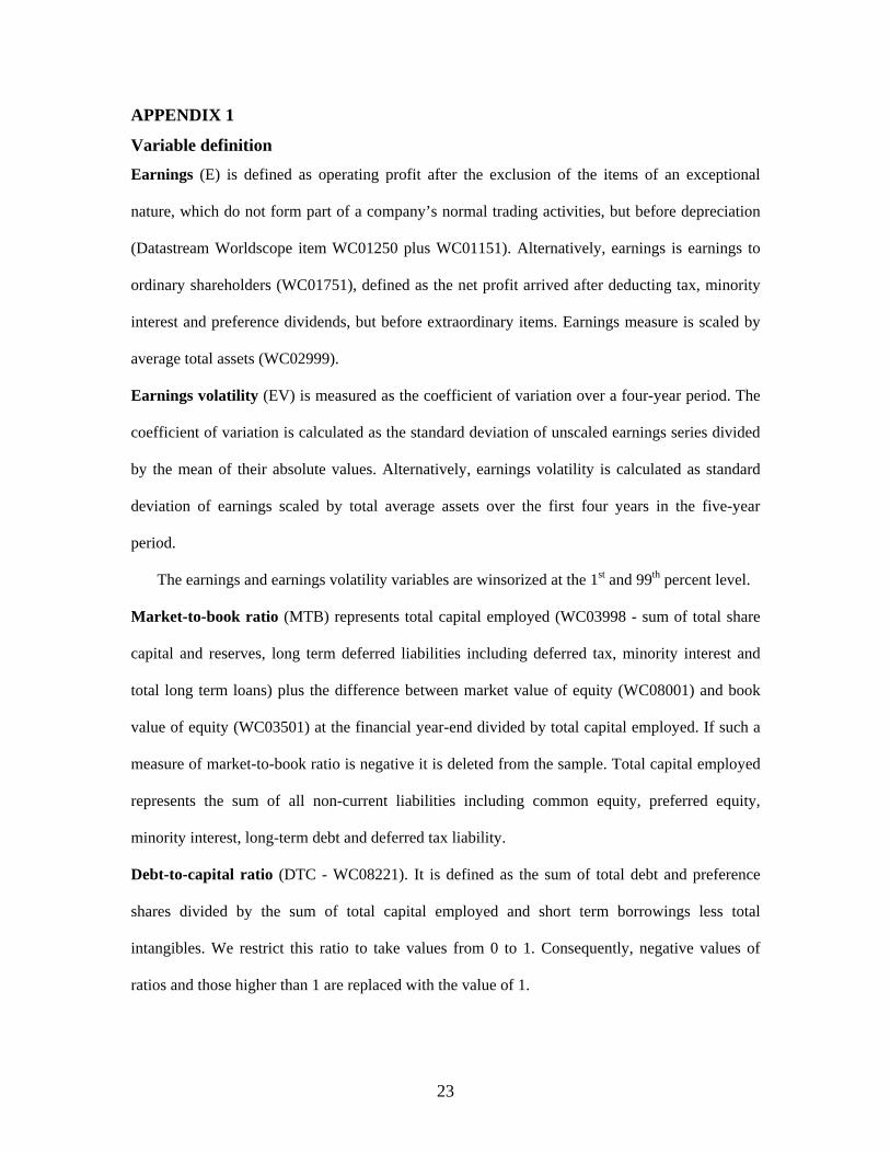
APPENDIX 1

Variable definition Earnings (E) is defined as operating profit after the exclusion of the items of an exceptional

nature, which do not form part of a company’s normal trading activities, but before depreciation

(Datastream Worldscope item WC01250 plus WC01151). Alternatively, earnings is earnings to

ordinary shareholders (WC01751), defined as the net profit arrived after deducting tax, minority

interest and preference dividends, but before extraordinary items. Earnings measure is scaled by

average total assets (WC02999).

Earnings volatility (EV) is measured as the coefficient of variation over a four-year period. The

coefficient of variation is calculated as the standard deviation of unscaled earnings series divided

by the mean of their absolute values. Alternatively, earnings volatility is calculated as standard

deviation of earnings scaled by total average assets over the first four years in the five-year

period.

The earnings and earnings volatility variables are winsorized at the 1st and 99th percent level.

Market-to-book ratio (MTB) represents total capital employed (WC03998 - sum of total share

capital and reserves, long term deferred liabilities including deferred tax, minority interest and

total long term loans) plus the difference between market value of equity (WC08001) and book

value of equity (WC03501) at the financial year-end divided by total capital employed. If such a

measure of market-to-book ratio is negative it is deleted from the sample. Total capital employed

represents the sum of all non-current liabilities including common equity, preferred equity,

minority interest, long-term debt and deferred tax liability.

Debt-to-capital ratio (DTC - WC08221). It is defined as the sum of total debt and preference

shares divided by the sum of total capital employed and short term borrowings less total

intangibles. We restrict this ratio to take values from 0 to 1. Consequently, negative values of

ratios and those higher than 1 are replaced with the value of 1.

23

Size (lnTA - total assets is Datastream item WC0299). It is measured as the average of natural

logarithm of total assets over four years. The logarithmic transformation is used to reduce the

impact of outliers.

Current ratio (CR - WC08106). This represents total current assets divided by total current

liabilities at the year-end.

Cash equivalents (CE – WC02001). This includes cash, bank balances, short-term loans and

deposits, and investments shown under current assets at the financial year-end scaled by average

total assets (WC0299).

MTB, DTC, lnTA and CR are calculated as an average value over the first four years in the

five-year period.

CR is winsorized at 1% and 99% level to control for outliers, while MTB, and CE are

winsorized at 99% level (they are bounded to zero at lower tail).

24

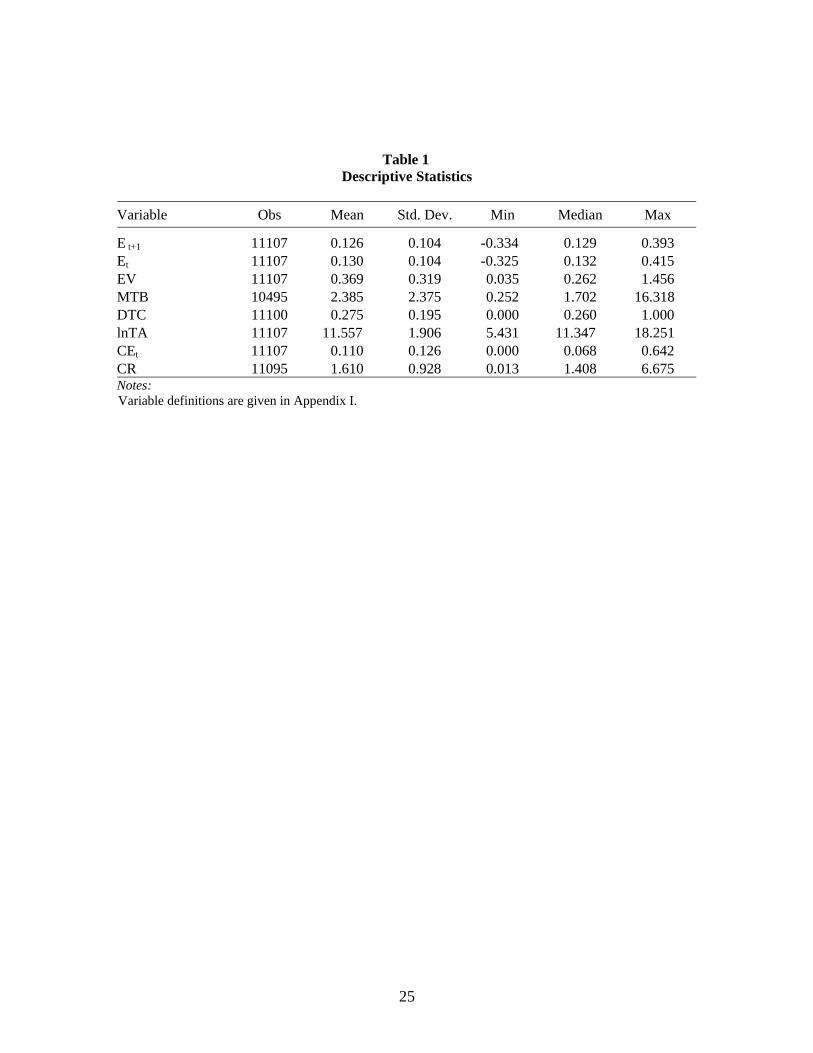
Table 1 Descriptive Statistics

Variable Obs Mean Std. Dev. Min Median Max

E t+1 11107 0.126 0.104 -0.334 0.129 0.393 Et 11107 0.130 0.104 -0.325 0.132 0.415 EV 11107 0.369 0.319 0.035 0.262 1.456 MTB 10495 2.385 2.375 0.252 1.702 16.318 DTC 11100 0.275 0.195 0.000 0.260 1.000 lnTA 11107 11.557 1.906 5.431 11.347 18.251 CEt 11107 0.110 0.126 0.000 0.068 0.642 CR 11095 1.610 0.928 0.013 1.408 6.675 Notes: Variable definitions are given in Appendix I.

25

Table 2 Correlation Matrix

Variables Et+1 Et EV(CV)

MTB DTC lnTA CEt-1 CR Et+1 1.0000Et 0.8297*

1.0000EV -0.3400* -0.3785* 1.0000MTB 0.0626* 0.1247* 0.0816* 1.0000DTC -0.0579* -0.0663* 0.1174* 0.0311* 1.0000lnTA 0.1616* 0.1576* -0.3707* -0.0988* 0.1746* 1.0000CEt -0.0811* -0.0591* 0.0545* 0.2894* -0.2250* -0.0996* 1.0000CR -0.2432* -0.2444* 0.1203* 0.0372* -0.3804* -0.2048* 0.4453* 1.0000Notes: Pearson correlation coefficients are reported below main diagonal. Variable definitions are given in Appendix I. * denotes statistical significance at the 1% level.

26

Table 3 Effects of adding earnings volatility to forecasting model of future one-year ahead earnings

(operating profit before depreciation) Model 1 Model 2 Model 3 Model 4

Intercept 0.0198 0.0238 0.0161 0.0070 (5.97)** (6.83)** (4.66)** (1.78)*

Et 0.8232 0.8179 0.9084 0.9559 (56.45)** (51.12)** (59.96)** (43.79)**

EV -0.0097 0.0195 (-2.08)* (2.51)**

Et *EV -0.2110 -0.3041 (-7.73)** (-6.29)**

Adjusted R2 0.6871 0.6900 0.6977 0.7025

Median F 3.44 13.15 12.69 (11/19) (16/19) (17/19) Mean AE 0.0360 0.0361** 0.0358 0.0357** Median AE 0.0220 0.0222 0.0220** 0.0217** Mean bias proportion -0.0000 0.0000 0.0000 -0.0001 Median bias proportion 0.0040 0.0034 0.0030** 0.0036** Mean APE 0.7763 0.7992 0.7177** 0.7754 Median APE 0.1625 0.1614 0.1647** 0.1614** Mean bias -0.4076 -0.4076 -0.3509** -0.4208 Median bias 0.0293 0.0240 0.0217** 0.0253** Notes: Sample consists of 11,107 observations for non-financial firms listed at London Stock Exchange with available data to calculate earnings volatility. Annual regressions are run for each year in the period from 1985 to 2003 for the following four models:

Model 1: ttt EE εβα ++=+ 11

ttt EVEE

Model 2: εββα +++=+ 211

tttt EVEEE

Model 3: εββα +++=+ *311

tt EVEEV

Model 4: tt EE ββα εβ ++++=+ 211 *3

The time-series mean coefficient estimates, corresponding t-statistics for the means (in parentheses), and the time-series mean adjusted R2 are reported. Median F-statistic testing the restriction that estimated coefficients on EV (Model 2), Et*EV (Model 3) and both EV and Et*EV, respectively, equal zero versus Model 1 is presented, with the number of annual F-statistics statistically significant at 10% given in parentheses. The coefficients estimated in year t are used to forecast earnings in year t+1. Forecasting was performed on the total sample available for year t+1 no matter whether the firms included are used for coefficient estimation purposes in year t. The following measures of out-of-sample forecast accuracy are calculated for 10,882 available observations in the period from 1986 to 2003. Absolute error (AE) is the absolute value of the difference between actual and predicted earnings. Bias proportion is the difference between the actual and predicted earnings. Absolute percentage error (APE) is the absolute value of the difference between the actual and forecasted earnings divided by the absolute actual earnings. Bias is the difference between the actual and forecasted earnings divided by absolute actual earnings. Mean and median of AE, APE, bias proportion and bias are reported. Variable definitions are given in Appendix I. ** and * denote statistical significance at the 5% and 10% levels, respectively. For the regression slopes, the teststatistic is two-tailed t-statistic that the coefficient means are statistically different from zero. For the measures offorecast accuracy and bias, the test statistic is t-statistic (Wilcoxon z-statistic) that the means (medians) in Models 2, 3and 4 are statistically different from mean (median) in Model 1.

27

Table 4 Cross-sectional analysis of earnings volatility and future one-year ahead earnings (operating profit before depreciation)

Alternative model

Benchmark model

MTB DTC lnTA CEt CR Intercept 0.0238 0.0161 0.0259 0.0168 0.0233 0.0279

(6.83)** (5.15)** (1.30)(6.19)** (6.85)**(6.55)**

Et 0.8179 0.8093 0.8186 0.8162 0.8154 0.8109(51.12)** (52.39)**(35.10)** (49.43)** (48.00)**(50.30)**

EV -0.0097 0.0100 -0.0151 -0.0083 -0.0025 -0.0146(-2.08)* (-2.38)**(1.55) (-0.25) (-0.42) (-1.67)

Char 0.0060 -0.0110 0.0006 0.0060 -0.0022 (3.24)** (-1.22) (0.70) (0.59) (-1.53)

Char*EV -0.0132 0.0261 0.0001 -0.0601 0.0042 (-3.37)** (1.25) (0.02) (-2.22)** (1.26)

Adjusted R2 0.6900 0.7001 0.6923 0.6928 0.6936 0.6928

Obs. 11107 11100

10495 11107

11107

11095

Mean AE 0.0361 0.0346 0.0364 0.0363 0.0361 0.0362 Median AE 0.0222 0.0216 0.0225 0.0222 0.0222 0.0222 Mean bias proportion 0.0000 -0.0001 0.0000 -0.0003 0.0001 0.0000 Median bias proportion 0.0034 0.0031 0.0033 0.0026 0.0031 0.0030 Mean APE 0.7992 0.7868 0.8201 0.8404 0.8257 0.8315 Median APE 0.1614 0.1579 0.1615 0.1619 0.1606 0.1619 Mean bias -0.4076 -0.4290 -0.4212 -0.4226 -0.4128 -0.4007 Median bias 0.0240 0.0224 0.0224

0.0188

0.0226

0.0204

N 10882 1087510288 10882 10882 10870

Notes: Sample consists of observations for non-financial firms listed at London Stock Exchange with available data to calculate earnings volatility and firm-specific characteristics. Annual regressions are run for each year in the period from 1985 to 2003 for two different types of models. Benchmark model is Model 2 from Table 3:

ttt EVEE εββα +++=+ 211

28

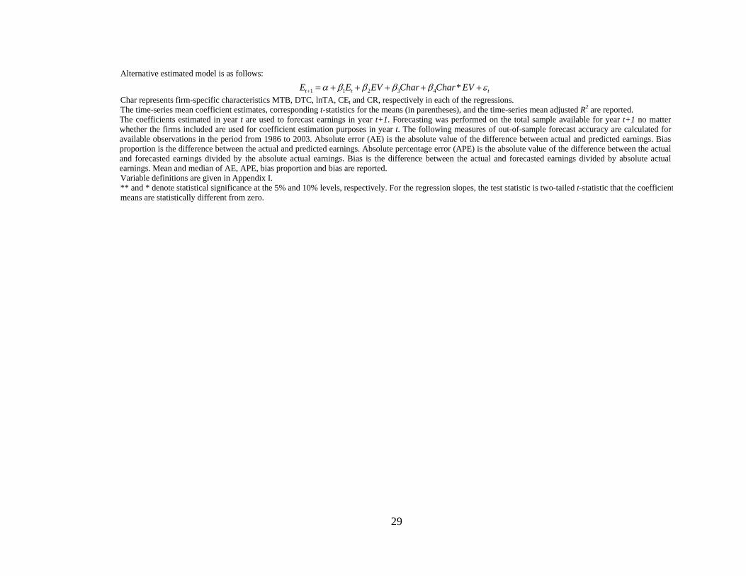
Alternative estimated model is as follows:

ttt EVCharCharEVEE εββββα +++++=+ *43211 Char represents firm-specific characteristics MTB, DTC, lnTA, CEt and CR, respectively in each of the regressions. The time-series mean coefficient estimates, corresponding t-statistics for the means (in parentheses), and the time-series mean adjusted R2 are reported. The coefficients estimated in year t are used to forecast earnings in year t+1. Forecasting was performed on the total sample available for year t+1 no matter whether the firms included are used for coefficient estimation purposes in year t. The following measures of out-of-sample forecast accuracy are calculated for available observations in the period from 1986 to 2003. Absolute error (AE) is the absolute value of the difference between actual and predicted earnings. Bias proportion is the difference between the actual and predicted earnings. Absolute percentage error (APE) is the absolute value of the difference between the actual and forecasted earnings divided by the absolute actual earnings. Bias is the difference between the actual and forecasted earnings divided by absolute actual earnings. Mean and median of AE, APE, bias proportion and bias are reported. Variable definitions are given in Appendix I. ** and * denote statistical significance at the 5% and 10% levels, respectively. For the regression slopes, the test statistic is two-tailed t-statistic that the coefficientmeans are statistically different from zero.

29

Table 5

Cross-sectional analysis of earnings volatility (standard deviation) and future one-year ahead earnings (operating profit before depreciation)

Alternative model

Benchmark model

MTB DTC lnTA CEt CR Intercept 0.0219 0.0163 0.0203 0.0119 0.0190 0.0252 (6.82)**

(6.75)** (6.00)** (1.11) (6.86)** (6.72)**

Et 0.8259 0.8211 0.8266 0.8218 0.8245 0.8193(56.47)** (56.14)**(38.08)** (53.08)** (52.99)**(54.60)**

EV -0.0781 0.0702 -0.0236 -0.0475 0.0483 -0.1420(-1.84)* (-0.53)(1.05) (-0.26) (0.97) (-1.37)

Char 0.0033 0.0053 0.0008 0.0183 -0.0018 (1.29)(1.88)* (1.24) (1.58) (-1.24)

Char*EV -0.0700 -0.2256 0.0013 -0.7982 0.0496 (-1.70)(-2.05)* (0.08) (-2.27)** (1.04)

Adjusted R2 0.6913 0.7015 0.6944 0.6940 0.6972 0.6948

Obs. 11107 11100

10495 11107

11107

11095

Mean AE 0.0359 0.0347 0.0362 0.0360 0.0359 0.0360 Median AE 0.0218 0.0217 0.0221 0.0218 0.0217 0.0219 Mean bias proportion 0.0001 0.0001 0.0002 -0.0002 0.0001 0.0001 Median bias proportion 0.0036 0.0038 0.0037 0.0029 0.0035 0.0032 Mean APE 0.7981 0.7740 0.8002 0.7996 0.8032 0.8105 Median APE 0.1595 0.1578 0.1605 0.1587 0.1585 0.1610 Mean bias -0.3994 -0.4255 -0.3949 -0.3953 -0.4075 -0.3885 Median bias 0.0259 0.0272 0.0261

0.0206

0.0253

0.0227

N 10882 1087510288 10882 10882 10870


30



ttt EVCharCharEVEE εββββα +++++=+ *43211 Char represents firm-specific characteristics MTB, DTC, lnTA, CEt and CR, respectively in each of the regressions. The time-series mean coefficient estimates, corresponding t-statistics for the means (in parentheses), and the time-series mean adjusted R2 are reported. The coefficients estimated in year t are used to forecast earnings in year t+1. Forecasting was performed on the total sample available for year t+1 no matter whether the firms included are used for coefficient estimation purposes in year t. The following measures of out-of-sample forecast accuracy are calculated for available observations in the period from 1986 to 2003. Absolute error (AE) is the absolute value of the difference between actual and predicted earnings. Bias proportion is the difference between the actual and predicted earnings. Absolute percentage error (APE) is the absolute value of the difference between the actual and forecasted earnings divided by the absolute actual earnings. Bias is the difference between the actual and forecasted earnings divided by absolute actual earnings. Mean and median of AE, APE, bias proportion and bias are reported. Variable definitions are given in Appendix I. ** and * denote statistical significance at the 5% and 10% levels, respectively. For the regression slopes, the test statistic is two-tailed t-statistic that the coefficient means are statistically different from zero.

31

Table 6 Cross-sectional analysis of earnings volatility and future one-year ahead earnings (earnings to ordinary shareholders)

Alternative model

Benchmark model

MTB DTC lnTA CEt CR Intercept 0.0175 0.0115 0.0263 0.0072 0.0185 0.0245 (3.77)**

(2.67)** (4.04)** (0.44) (4.43)** (5.06)**

Et 0.6491 0.6647 0.6408 0.6453 0.6349 0.6416(15.65)** (15.19)**(15.31)** (15.00)** (14.88)**(15.06)**

EV -0.0141 -0.0189

-0.0051 -0.0419 -0.0166 -0.0200(-3.39)** (-3.24)**(-0.95) (-2.03)* (-2.97)** (-2.45)**

Char 0.0030 -0.0372 0.0008 0.0014 -0.0038 (2.35)** (-3.32)** (0.75) (0.07) (-1.37)

Char*EV -0.0049 0.0263 0.0026 0.0199 0.0034 (2.01)*(-1.49) (1.57) (0.83) (0.86)

Adjusted R2 0.4060 0.4289 0.4123 0.4113 0.4116 0.4121

Obs. 11108 11101

10496 11108

11108

11093

Mean AE 0.0562 0.0525 0.0565 0.0564 0.0563 0.0564 Median AE 0.0277 0.0262 0.0285 0.0277 0.0282 0.0278 Mean bias proportion 0.0006 0.0003 0.0007 0.0008 0.0004 0.0007 Median bias proportion 0.0103 0.0102 0.0103 0.0096 0.0101 0.0097 Mean APE 2.3416 2.2018 2.3588 2.5545 2.3641 2.4819 Median APE 0.4102 0.3891 0.4246 0.4039 0.4110 0.4096 Mean bias 0.5165 0.4404 0.5653 0.6149 0.5137 0.5926 Median bias 0.1474 0.1465 0.1492

0.1384

0.1462

0.1367

N 10883 1087610289 10883 10883 10868



32


ttt EVCharCharEVEE εββββα +++++=+ *43211 Char represents firm-specific characteristics MTB, DTC, lnTA, CEt and CR, respectively in each of the regressions. The time-series mean coefficient estimates, corresponding t-statistics for the means (in parentheses), and the time-series mean adjusted R2 are reported. The coefficients estimated in year t are used to forecast earnings in year t+1. Forecasting was performed on the total sample available for year t+1 no matter whether the firms included are used for coefficient estimation purposes in year t. The following measures of out-of-sample forecast accuracy are calculated for available observations in the period from 1986 to 2003. Absolute error (AE) is the absolute value of the difference between actual and predicted earnings. Bias proportion is the difference between the actual and predicted earnings. Absolute percentage error (APE) is the absolute value of the difference between the actual and forecasted earnings divided by the absolute actual earnings. Bias is the difference between the actual and forecasted earnings divided by absolute actual earnings. Mean and median of AE, APE, bias proportion and bias are reported. Variable definitions are given in Appendix I. ** and * denote statistical significance at the 5% and 10% levels, respectively. For the regression slopes, the test statistic is two-tailed t-statistic that the coefficientmeans are statistically different from zero.

33

Does Volatility Improve UK Earnings Forecasts&quest

Documents

Transcript of Does Volatility Improve UK Earnings Forecasts&quest