Does Public Ownership of Equity Improve Earnings Quality?

Dan Givoly*, Carla Hayn** and Sharon P. Katz***

April 17, 2007

* The Pennsylvania State University; ** University of California, Los Angeles; *** Harvard University We are grateful for the useful comments by Bjorn Jorgensen, Doron Nissim and Stephen Penman, as well as the participants of the U.S. Securities and Exchange Commission and accounting workshops at Columbia University and Washington University.

Does Public Ownership of Equity Improve Earnings Quality?

Abstract

To better understand how equity investors influence earnings quality, we compare the quality of accounting numbers produced by two types of public firms – those with publicly-traded equity and those with privately-held equity that are nonetheless considered public by virtue of having publicly-traded debt. We develop and test two hypotheses. The “demand” hypothesis holds that earnings of public equity firms are of higher quality than earnings of private equity firms due to the stronger demand by investors and creditors stemming from, among other concerns, higher litigation risk. The “opportunistic behavior” hypothesis posits that public equity firms have lower earnings quality than their private equity peers due to management intervention in the earnings process as a result of capital market considerations as well as their own equity-based compensation. We identify a number of attributes associated with the notion of earnings quality – persistence and estimation error of accruals, prevalence of earnings management, timeliness of loss versus gain recognition (conditional conservatism) and the extent of conservatism due to the use of asset-decreasing accounting principles (unconditional conservatism). The results indicate that, consistent with the “opportunistic behavior” hypothesis, private-equity firms have higher quality accruals and a lower propensity to manage income than public equity firms. However, in line with the “demand” hypothesis, public equity firms’ financial reports are generally more conservative.

Does Public Ownership of Equity Improve Earnings Quality?

1. Introduction

The quality of accounting information is influenced by an array of factors, most of which

relate to the demand for such information for use in contractual arrangements and to the

incentives and opportunities of management to tamper with the reported numbers. Both the

demand for quality accounting information and management incentives to manage earnings

depend on whether the equity of the company is privately or publicly traded. Examining the

differential accounting quality between private equity and public equity firms thus sheds light on

the influence of these factors.

Several studies such as Beatty et al. (2002) and Penno and Simon (1986) explore how the

ownership structure, public or private, influences the quality of accounting numbers. Because

financial data of privately-owned firms is generally unavailable, these studies are restricted to

regulated industries such as banking and insurance where financial reports of both public and

private companies are filed with industry regulators. Their results, while insightful, cannot be

easily generalized due to the industry concentration of the samples as well as the uniqueness of

the financial reporting issues in these industries. Ball and Shivakumar (2005) and Burgstahler,

Luzi and Leuz (2006) compare the earnings quality of public and private firms in Europe where

private companies must file financial statements. Since their studies are not limited to regulated

industries, the results are more generalizable but the extent to which they apply to U.S. firms is

not clear due to differences in these countries reporting regimes.1

Our study extends the literature on the factors affecting the quality of accounting

numbers by comparing the quality of accounting information as a function of the ownership

structure. Specifically, we compare the accounting quality of two types of public companies:

those with publicly-traded equity (hereafter, public equity firms) and those with privately-held

equity that are still considered public companies due to their publicly-traded debt (hereafter,

private equity firms). Both types of firms in our sample operate in the U.S. and are subject to

identical reporting and disclosure requirements. Hence, our analysis controls for many of the

1 A related line of research explores the factors that influence the accounting quality of publicly-traded firms across countries. These international comparisons examine various quality attributes of accounting information, particularly conservatism (e.g., Ball, Kothari and Robin (2000), Ball, Robin and Wu (2003), Bushman and Piotroski (2004) and Pope and Walker (1999)).

2

factors affecting the comparison of earnings quality across countries such as legal institutions,

tax laws, securities regulation and the extent of their enforcement, as well as reporting and

disclosure requirements. As a result, we are able to focus more precisely on how the ownership

structure of the company affects its accounting quality.

The paper shows that the difference in reporting quality between public equity firms and

private equity firms that are public companies by virtue of having publicly-traded debt exhibit

different reporting attributes. However, neither group “dominates” the other in terms of having

higher overall quality reporting. Public equity firms generally report more conservatively, one

dimension of reporting quality. However, private equity firms’ financial reports exhibit

considerably less earnings management, another dimension of reporting quality.

The paper is the first to analyze the quality of accounting information generated by firms

whose debt, but not equity, is publicly traded. It provides information about the differential

demand for earnings quality by public equity holders and public debt holders of private equity

firms. It further examines the different incentives and opportunities that management of these

two types of corporations has to affect the reported numbers.2 The paper extends the literature on

earnings quality and the differential quality between public versus private companies, thus

enhancing our understanding of how, and the extent to which, management incentives and

investors’ demand for earnings quality impact financial reporting.

The paper contributes to the existing literature in two main respects. First, rather than

focusing on a single dimension of earnings quality such as conservatism, a broad spectrum of

“earnings quality” attributes are considered. Second, by examining a unique sample of privately-

held public companies, the study highlights how the presence of equity investors affects

management’s reporting behavior, controlling for the regulatory environment as well as the

disclosure and reporting regimes.

The remainder of the paper is organized as follows. The next section describes the

characteristics of this unique sample of firms that have public debt and private equity. The

hypotheses are developed in the third section, followed by a discussion of the various measures

of accounting quality used in the paper. The sample and data are described in section 5. Results

are provided in section 6. The last section of the paper contains concluding remarks.

2 As explained later in the paper, in order to focus directly on the impact of equity ownership, we control for the role of public debt by including in our sample of public equity firms only those with public debt.

3

2. Private Equity Firms with Public Debt

Under Sections 13 and 15(d) of the Securities Exchange Act of 1934, firms with publicly-

traded equity as well as those with privately-owned equity and publicly-traded debt are subject to

identical financial reporting regulations. While both are considered to be public firms and are

subject to the same reporting and disclosure requirements, the latter group of private equity firms

is distinctly different from public equity firms because their ownership is not traded. Therefore

equity-based compensation is rare and takeovers through open market stock purchases are not

possible.

Similar to holders of public debt in public equity firms, the holders of public debt in

private equity firms are protected by the Trust Indenture Act of 1939. This act requires that firms

receive the unanimous consent of the public debt holders in order to modify the terms of the

bond indenture agreements. Given the dispersed holdings of most bond issues, this unanimity

requirement is likely to make it difficult to renegotiate public debt. Accordingly, this regulation

is viewed as providing public debt holders with less effective monitoring and less flexible debt

renegotiation as compared to that provided by private lenders.3

The factors leading private equity owners to issue public debt before they issue public

equity, while having a bearing on the “pecking order” theory, have not been directly researched.

However, research on the priority of financing sources suggests that issuing public debt involves

more costly disclosure of propriety information than does issuing private debt (Campbell (1979),

Myers (1984) and Yosha (1995)). Other things being equal, one would thus expect firms to rely

more on private debt when the public disclosure of firm-specific information is costlier.4

Empirical evidence further suggests that credit quality plays a role in firms’ debt financing

choices. Specifically, firms with higher credit ratings tend to borrow from public sources, those

with intermediate ratings borrow from banks, and firms with the lowest credit quality borrow

from private lenders (Denis and Mihov (2003)). These findings suggest that firms that issue

public debt are likely to be financially stronger than firms that do not have publicly held debt, an

expectation borne out by our sample firms (as discussed in section 6).

3 Smith and Warner (1979) discuss the typical contractual arrangements of public versus private debt. 4 Dhaliwal et al. (2004) review the theory and empirical evidence on public versus private debt.

4

3. Hypotheses on Earnings Quality and Ownership Structure

A natural starting point for developing hypotheses about the quality of financial reporting

of the private equity firms with publicly traded debt is the hypotheses developed by previous

research on the differential quality of financial reports for public versus private firms.

Interestingly, these hypotheses lead to conflicting predictions. On one hand, the demand for high

quality reporting by public equity firms is hypothesized to be stronger since accounting

information is the only type of information contractually available to public equity holders. In

contrast, debt holders, particularly holders of private debt, may have access to other, nonpublic

information on the firm’s performance. Further, debt holders typically have disciplining

mechanisms beyond those available to equity holders. In addition to contractual concerns, public

equity firms may take efforts to improve the accounting and disclosure policies in order to

mitigate potential lawsuits, in keeping with the findings of Skinner (1997). Based on these

considerations, the demand for quality accounting information is expected to be greater for

public equity firms than for private equity firms. This “demand” hypothesis is advanced by Ball

and Shivakumar (2005) and, by implication, studies on the differential demand for financial

reporting quality between countries that resolve information asymmetries via “insider access” and

countries that alleviate the asymmetries through “arm’s length” public disclosures.5

On the other hand, management of public firms is under continuous pressure by investors

to meet certain performance benchmarks. For example, management has incentives to manage

stock prices to meet analysts’ forecasts (e.g., Bartov et al. (2002)) or to avoid reporting losses

(e.g., Hayn (1995) and Burgstahler and Dichev (1997)) or earnings decreases (e.g., Barth et al.

(1999)). Further, management may have a personal stake in the firm’s stock price arising from

stock-based compensation. For these reasons, accounting quality of pubic equity firms may be

lower than that of private equity firms if earnings are managed with an eye to achieving higher

stock prices. This “opportunistic behavior” hypothesis is supported by the findings of Beatty et

al. (2002) and the survey results of Penno and Simon (1986).

5 International evidence is consistent with insider access and high quality public financial reporting being substitutes for reducing information asymmetries. Similar evidence is provided by Ball and Shivakumar (2005) with respect to private companies (where there is a greater insider access) and public companies (shown to have a higher quality of financial reporting).

5

The “demand” and “opportunistic behavior” hypotheses are not mutually exclusive and

may, in fact, both be valid. The observed differential in financial reporting quality likely reflects

the net effect of the two influences.

The demand for accounting quality created by having public equity (as compared to

private equity) is similar to the effect created by having public debt (as compared to private

debt). In terms of this demand, note that in private equity firms, the public debt holders have less

access to private information, less effective ways of monitoring and disciplining management,

and less efficient tools for liquidation or renegotiations in the event of financial distress than are

available to private lenders. Unlike private lenders, public debt holders are not privy to inside

information before extending credit nor are they entitled to receive information on the extent of

compliance with the terms of the debt contract beyond that contained in the prospectus and in

subsequent SEC-mandated public reports and disclosures.6 As a result of these differences,

public debt holders in private equity companies suffer an information disadvantage relative to the

owners that is very similar to that suffered by public equity holders relative to insiders. For this

reason we expect the demand for quality reporting by public debt holders in private equity firms

to be stronger than that of private debt holders.

Regarding the “opportunistic behavior” hypothesis, managers of private equity firms are

likely to have weaker incentives to manipulate earnings than their peers in public equity firms

since capital market considerations are not a concern (except, perhaps, in situations where a firm

is on the brink of violating its debt covenants). Further, managers of private equity firms would

not have strong compensation-related incentives to manage earnings since their pay is unlikely to

be tied to the value of the firm’s stock (which is not traded).

Because the “demand” hypothesis predicts no difference between the two groups of firms

while the “opportunistic behavior” hypothesis predicts a higher earnings quality (lower

likelihood of earnings management) for the private equity firms as compared with public equity

firms, comparing the earnings quality attributes of these two groups of public firms provides a

6 Theory and empirical evidence suggest that access to information and the strength of the monitoring mechanism is likely to differ between public and private debt. Previous studies hypothesize, for example, that private debt financing has an advantage over public debt in terms of monitoring efficiency (e.g., Diamond (1984); Boyd and Prescott (1986); Berline and Loyes (1988)), access to private information (Fama (1985)) and the efficiency of liquidation and renegotiation in financial distress (Chemmanur and Fulghieri (1994); Gertner and Scharfstein (1991)). The empirical evidence is generally consistent with these expectations (e.g., Kwan and Carlton (2003)). Johnson (1997) provides a summary of these findings.

6

cleaner and more powerful test of the latter hypothesis than do comparisons between private and

public firms in general.

Note further that the demand for accounting quality as well as the opportunistic behavior

of managers of public-equity firms may be affected by whether they have public debt. To control

for these effects, we compare the accounting quality of private equity firms with public debt to

that of public equity firms with public debt.

The predictions of the two hypotheses with respect to accounting quality of firms with

different types of stakeholders are summarized in the following table. For completeness, we also

include the predictions for the group of entirely private firms (private equity and private debt) for

which no information is publicly available in the U.S. 7

Type of Stakeholders

“Demand” Hypothesis

Predicted Quality of Financial Reporting

“Opportunistic Behavior” Hypothesis

Predicted Quality of Financial Reporting

1. Private equity, private debt

Weak demand for quality external reporting

Low No incentive to manage accounting numbers High

2. Private equity, public debt

Strong demand for quality external reporting from debt holders

Medium

Limited incentives to manage accounting numbers Medium

3. Public equity, public debt

Very strong demand for quality external reporting from both equity and debt holders

High

Strong incentives to manage accounting numbers Low

In comparing the quality of accounting numbers between private equity, public debt firms

(the second group) and public equity firms (the third group), it is important to note that the

choice between public and private debt is endogenous and positively associated with firm

characteristics such as size, leverage, age and amount issued (Houston and James (1996),

Johnson (1997), Krishnaswami, Spindt and Subramaniam (1999) and Cantillo and Wright

(2000)). Further, both theoretical models and the empirical evidence suggest that firms with the

7 Private equity firms with private debt that have more than 500 investors and $10 million in net assets are required to file reports with the SEC (http://www.sec.gov/investor/pubs/cyberfraud.htm). However, the vast majority of these firms are cooperatives, which may differ in terms of earnings management and quality of reporting due to differences in organizational and ownership structures.

7

highest credit quality tend to borrow from public sources whereas poor quality borrowers rely

more on private debt (Cantillo and Wright (2000); Denis and Mihov (2002)). This discussion

suggests that in testing for differences in financial reporting quality between private equity firms

and those public equity firms without public debt, it is important to control for an array of factors

(e.g., size, and leverage) that are likely to affect both the public-private debt choice as well as

earnings quality.

4. Measures of Accounting Quality

No single measure of the quality of accounting numbers captures all of the dimensions of

quality. Previous studies have identified a number of attributes associated with different aspects

of earnings quality such as accrual persistence, estimation errors in the accrual process, absence

of earnings management and conservatism. These four quality attributes are discussed in the

following paragraphs.

4.1. Accrual persistence

Our first measure of earnings quality views the differential persistence of accruals

relative to cash flows as an indication of earnings quality. This earnings quality measure has

been used by Sloan (1996) and articulated by Richardson et al. (2005) as “the degree to which

earnings performance persists into the next period.” Persistence is gauged using the following

regression:

OIi,t+1 = α +β1 CFi,t + β2 ACCRi,t + εi,t, (1)

where i and t are, respectively firm and time subscripts and OI is operating income after

depreciation, CF is the cash flow component defined as OI – ACCR, and ACCR is the accrual

component measured as the change in net operating assets (NOA) from t-1 to t. 8 All variables in

equation (1) are standardized by NOAt-1. The incremental contribution of accruals is determined

by the magnitude and significance of β2.

We account for the possible endogeneity of the choice to issue private or public equity by

using the Heckman (1979) two-stage procedure. In the first stage, size (measured alternatively as

total assets and sales), growth in sales, leverage (defined as total debt divided by total assets),

profitability (defined as operating income over net operating assets, RNOA), and the quick ratio 8 Net operating assets equal the book value of common and preferred equity, plus total debt, minus the sum of cash, short-term investments and investment and advances, plus minority interest (see Nissim and Penman (2003)).

8

serve as predictors of the equity choice in a PROBIT model. Estimates of the PROBIT model are

used to compute the inverse Mills ratio for each sample firm. In the second stage, we include the

inverse Mills ratio as a control variable in regression (1), allowing the coefficient to vary

between the two groups of firms.

4.2. Estimation error in the accruals process

Accruals are estimates of future cash flows. To the extent that the accruals process is free

of estimation error, accruals and earnings will be more representative of future cash flows. The

second attribute of earnings quality is thus the degree of stability in the relation between cash

flows and accruals. A measure used to assess the degree of stability was proposed by Dechow

and Dichev (2002) and further modified by Francis et al. (2005). Specifically, the measure is

based on the variance of the residuals from the following model (which represents a modification

introduced by McNichols (2002)):

TCAi,t = β0 +β1CFOi,t-1 + β2CFOi,t + β3CFOi,t+1 + β4ΔRevi,t + β5PPEi,t + εi,t (2)

where i and t are firm and time subscripts, respectively, TCA is total current accruals,9 CFO is

cash flows from operations, ΔRevt is the change in revenues from year t-1 to t and PPE is the

balance of property, plant and equipment (on a gross basis). Cash flow from operations is

measured as income from continuing operations less total accruals (i.e., total current accruals

minus the depreciation and amortization expense). All variables are scaled by average total assets

in year t.

Following Francis et al. (2005), we estimate equation (2) cross-sectionally for each

industry with at least 20 observations in a given year. Industries are defined based on two-digit

SIC codes. The quality measure is the variability (standard deviation) of the residuals from the

above regression. Specifically, the higher is the variability the lower is the quality of the accruals

and, correspondingly, earnings.

Because the standard deviation of the accruals may reflect the volatility of the firm’s

operations rather than reporting quality per se (Liu and Wysocki, 2006), we follow the

suggestion in Verdi (2006) and create an additional relative measure of accruals quality defined

9 Total current accruals equal operating assets (current assets excluding cash and short term investments) minus operating liabilities (current liabilities excluding the current portion of long-term debt).

9

as the ratio of the standard deviation of the residuals from equation (2) to the standard deviation

of total current accruals.10

4.3. Absence of earnings management

It is difficult to determine the presence or absence of earnings management since the

series of unmanaged earnings is not observable. However, certain patterns in earnings are

indicative of the presence of earnings management. One such pattern is the concentration of

earnings numbers just above some earnings threshold. For example, earnings clustered just above

zero have been interpreted as reflecting earnings management to avoid reporting a loss. Earnings

growth in the current quarter relative to the same quarter the previous year of zero or slightly

positive may suggest that the current period’s earnings have been managed to avoid reporting an

earnings decline. Similarly, earnings that result in no, or just a small, positive earnings surprise

are often viewed as having been managed to meet or just beat analysts’ earnings forecasts.

In line with Burgstahler and Dichev (1997), we identify earnings management cases as

those where the observed relative frequency of earnings being just above (just below) an

earnings threshold exceed (fall below) their theoretical values. For the purpose of this analysis,

we divide the distribution of the earnings measure into “bins” with bin widths determined by the

formula suggested by Degeorge et al. (1999) and test for the significance of the difference

between the actual and theoretical frequency in a bin based on the procedure proposed by

Burgstahler and Dichev (1997).11 For the statistical tests on the difference, we calculate the

standardized differences for the interval just below zero, and the interval just above zero. Under

the assumption of no earnings management, the expected number of observations in any given

interval is equal to the average of the number of observations in the two adjacent intervals. If

managers succeed in meeting the threshold, we would expect to find a shift of observations from

the bins just below the earnings threshold to the bins just above that threshold.

10 Francis et al. (2005) and Verdi (2006) further differentiate between the component of accruals quality driven by operational characteristics of the firm over which management has limited control (such as the length of the operating cycle or firm size) and the discretionary component which reflects managerial choices. Because our comparison is done within industries, controlling for the operational characteristics is less important. Further, because our basic observation is the industry/type of firm, our sample is fairly small (55 industries for the public equity sample and 24 industries for the private equity sample) making it difficult to obtain a reliable estimate of this “firm-characteristics-adjusted” accrual quality measure. 11 The bin width, BW, is determined as BW = 2(IQR)n-1/3, where IQR is the sample inter-quartile range and n is the number of observations. To test the significance of the difference between the theoretical and actual relative frequencies in a bin, we evaluate the difference deflated by the estimated standard error of the difference. The standard error is based on a variance estimate of N*Pi*(1 – Pi) + [(1/4)*N*(Pi-1 + Pi+1)(1 - Pi-1 - Pi+1)], where N is the total number of observations and Pi is the probability that an observation will fall into interval i.

10

A number of studies expressed concerns regarding the effectiveness of this procedure to

identify earnings management (e.g., Durtschi and Easton (2005); Beaver, et al. (2004); Dechow,

et al. (2003)). To increase the confidence in the identification of cases “just above” the

thresholds as earnings management cases, we follow Dechow et al. (2003) and investigate

whether cases in the bins just above the threshold have a higher proportion of positive

unexpected discretionary accruals. To even more precisely pinpoint earnings management cases,

we examine the percentage of the positive unexpected accruals cases where these accruals “made

the difference,” that is their magnitude was sufficiently positive so as to turn an otherwise loss

into a small profit. We identify “expected” or “nondiscretionary” accruals using the modified

Jones model.12

4.4. Conservatism

Another dimension of earnings quality is the extent of reporting conservatism.

Conservatism may take the form of a more timely recognition of economic losses as compared

with the recognition of economic gains or of a systematic undervaluation of assets. In either case,

it results in a systematic undervaluation of the book value of the equity relative to its economic

value (see Watts (2002) and Givoly et al. (2007)). Note that while capital market and

compensation considerations may lead public equity firms to manage earnings and thereby

introduce greater estimation error in accruals, such considerations are unlikely to result in a

lower level of conservatism. In fact, the higher level of litigation risk faced by public equity

firms and their management may induce a greater degree of conservatism through an earlier

recognition of losses.13

From the demand side, the information asymmetry between shareholders and

management creates a demand for a greater degree of conservatism in public equity companies

relative to those with private equity (Ball and Shivakumar (2005)). Our expectation therefore is 12 Specifically, we estimate the following regression cross-sectionally within each 2-digit SIC code industry: TACCj,t = a1*[1 / TAj, t-1] + a2*[(ΔREVj, t - ΔTRj, t ) / TAj, t-1] + a3*[PPEj, t / TAj, t-1] where TACCj,t is total accruals of firm j in year t, defined as the difference between income from continuing operations and net cash flow from operating activities, adjusted for extraordinary items and discontinued operations. TAj,t-1 is the beginning-of-the-year total assets. ΔREVj,t is the change in sales in year t. PPEj,t is gross property, plant and equipment in year t. ΔΤRj,t is the change in trade receivables in year t. For the years prior to 1988, when data on cash flows are unavailable, we define total accruals as follows: Δ(current assets) - Δ(current liabilities) - Δ(cash) + Δ(short-term debt) - (depreciation and amortization). To correct for measurement errors in this “balance sheet approach” (see Hribar and Collins (2002)), we eliminate firm-year observations with "non-articulating" events, namely: mergers or acquisitions, discontinued operations, and gains or losses on foreign currency translations. 13 For example, Skinner (1994, 1997) and Kasznik and Lev (1995) explore management incentives to issue earnings warnings.

11

that public equity firms will exhibit a higher degree of reporting conservatism than will private

equity firms.

We use two measures two capture the extent of a company’s reporting conservatism. The

first relates to the differential timeliness of loss versus gain recognition. The second assesses the

hidden reserves created as a result of using conservative accounting principles.

The speed in which earnings reflect bad news as compared with good news is a measure

of conservatism that has been employed by a number of studies (e.g., Basu (1997) and Ball and

Shivakumar (2005)). In the context of our study, we hypothesize that, because of a greater

demand for earnings quality from their shareholders, public equity companies will recognize

economic losses (bad news) in a timelier manner than will private equity companies. To capture

the differential timeliness of the earnings response to bad versus good news, we use a measure

that captures the relative persistence of losses and gains. This measure is estimated as the

coefficient α3 from the following piecewise linear regression:

ΔNIi,t = α0 + α1DΔNIi, t-1 + α2ΔNI i, t-1 + α3DΔNI i, t-1*ΔNI i, t-1 + ε i, t-1 (3)

where i and t designate the firm and time period, ΔNI is change in income (alternatively defined

as including and excluding extraordinary and exceptional items) from fiscal year t-1 to t, scaled

by the beginning book value of total assets. DΔNI is a dummy variable set equal to one if the

prior-year ΔNI is negative and zero otherwise.

Deferring the recognition of gains until their related cash flows are realized causes gains

to be a “persistent” positive component of accounting income that tends not to reverse. The

implication of this is that α2 is expected to equal zero. In contrast, the timely recognition of

economic losses implies that they are recognized as transitory income decreases, which results in

subsequent earnings reversal. This implies that α2 + α3 < 0. The hypothesis that economic losses

are recognized in a more timely fashion than gains implies that α3 < 0.

Similar to Ball and Shivakumar (2005), our hypothesis is that public equity firms are more

likely to recognize economic losses in a timely fashion than private equity firms. As in the

estimation of regression (1), we account for the possible endogeneity by using the Heckman

(1979) two-stage procedure that involves the estimate of a PROBIT model and the determination

of the inverse Mills ratio in the first stage and the inclusion of that ratio as a control variable in

regression (3) (see section 4.1).

12

We use two other measure of conservatism, the C- and Q-scores, developed by Penman

and Zhang (2002). These measures capture the effect on the balance sheet and income statement

of the “hidden reserves” arising from the application of conservative accounting methods such as

LIFO or expensing (rather than capitalizing) investments in intangible assets such as R&D and

advertising. The C-score is estimated as:

C-scorei,t = (INVi,tres + RDi,t

res + ADVi,tres) / NOAi,t-1 (4)

where INVres is the value of the LIFO reserve, RDres is the research and development reserve

calculated as the estimated value of R&D assets that would have been reported on the balance

sheet had R&D not been expensed, and ADVres is the advertising reserve estimated as the brand

assets created by advertising expenditures. To determine the (hypothetical) R&D assets, we

“capitalize” the annual R&D expenditures and amortize them using the sum-of-the-years’ digits

method over a five-year period. We use a similar approach to estimate the advertising reserve,

“capitalizing” advertising expenses and amortizing them using the sum-of-the-years’ digits

method over a two-year period. The sum of these three reserves is standardized by the value of

net operating assets at the end of the prior year.14

The second conservatism measure proposed by Penman and Zhang is an industry -

adjusted C-score, denoted as the Q-score. The Q-score is defined as the firm’s C-score minus the

median C-score of the firm’s industry.

5. Sample

Using the Compustat database (industrial, full coverage and research), we first identify

observations (firm-years) during the 26-year period from 1978-2003 that are likely to be private

equity, public debt firms using the following criteria:15

(1) the firm’s stock price at yearend is unavailable,

(2) the firm has outstanding debt (Compustat items #9 + #34) exceeding $1 million or is

designated as having gone through an LBO or become private,

(3) the firm is a separate, domestic company (and not a subsidiary of another public firm),

(4) the firm has at least $1 million in revenues and

(5) the firm has the financial data need to test the hypotheses for at least two years. 14 Net operating assets equal the book value of common and preferred equity, plus total debt minus the sum of cash, short-term investments and investment and advances, plus minority interest (see Nissim and Penman (2003)). 15 Our starting point was 1978 since our searches suggest that the first private equity firm to issue public debt was most likely Movado Group, Inc. in 1979.

13

We exclude firms in the financial industry (SIC codes between 6000 and 6999) and other

regulated industries (SIC codes between 4800 and 4900).

The resulting initial sample consists of 2,817 distinct firms and 12,261 firm-year

observations. Since some public equity firms met the above criteria as a result of missing price

data (criterion 1 above), we separately examined each firm to ensure that it had private equity

and publicly-traded debt in the identified time period. This examination resulted in eliminating

approximately 80% of the initial sample. We further eliminated some firms because their

organizational and ownership structures made it likely that their reporting policies and

management incentives would differ from those of private equity, public debt firms in general.

Specifically, we eliminated 21 firms structured as cooperatives or subsidiaries of cooperatives

(302 firm-year observations), 3 limited partnerships (27 firm-year observations) and 2

government owned firms (16 firm-year observations). The final private equity sample consists of

531 distinct firms (2,519 firm-year observations).16

To construct a sample of public equity firms, we identified firms in the same time period

that met criteria (2) through (5) described above. In addition we required that, similar to their

private equity counterparts, the public equity firms in our sample have publicly-traded debt. The

presence of public debt in a given year is established based on one of the following indications:

(1) availability of S&P senior debt ranking (Compustat item #280), (2) existence of debt

debentures (#82) or (3) issuance of public debt (according to Mergent Fixed Income Securities

database (FISD)) prior to the observation year with a maturity date beyond the observation year.

Applying the above criteria resulted in a final sample of 3,954 distinct public equity firms

(30,696 firm-year observations) with publicly-traded debt.

Public equity and private equity firms may have different attributes in addition to

ownership type that are likely to affect earnings quality. To control for the effect of these

attributes, such as firm size, we use a matched-pairs sample in some of our analyses. This sample

is constructed by matching each private equity firm with a public equity firm in the same

industry and of a similar size. To form this matched sample, we rank all firms (public equity and

private equity) based on their total assets at each yearend. We then partition the sample into

16To determine whether the firms qualified as private equity firms, we used data in the SEC filings on the EDGAR database (since 1993) and information on 10K Wizard (prior to 1993), bankruptcy information from BankruptcyData.com, and other historical information in the Hoover’s database as well as several news resources including Factiva, ProQuest and LexisNexis.

14

deciles to form ten firm-size portfolios. Each of the 2,519 firm-years in the private equity

sample is then matched with an observation in the public equity firm sample drawn from the

same size portfolio that (a) is the same year, (b) has the same 3-digit SIC code and (c) is closest

in size to the private equity firm observation. The resulting sample, which we refer to as the

“matched-pair sample” consists of 1,212 matched pairs of private equity and public equity firms.

6. Results

6.1. Descriptive statistics of the private equity, public debt firm sample

Table 1 provides descriptive statistics on financial and other characteristics of the private

equity, public debt firm sample which, as noted above, consists of 531 firms, representing 2,519

firm-years.17 Panel A shows the distribution of the firms by owner. The ownership structure

suggests that the impetus for privately-owned companies to issue debt is either a leveraged

buyout (LBO) generally by a financial sponsor or a management buyout (MBO). For example,

the equity of Levi Strauss & Co., a privately-held company with public debt, was taken private in

1985 through an MBO. The equity of Sealy Corporation, another company with public debt, was

taken private through an LBO in 1989. Financial sponsors are investment firms such as The

Blackstone Group, Texas Pacific Group and Kohlberg Kravis Roberts & Co. (KKR). In contrast

to venture capital firms which often invest in early-stage companies, financial sponsors generally

buy mature businesses via LBOs and MBOs transactions.

As panel B shows, the private equity firms have a similar industry representation as the

sample of public equity firms. Further, there is no particular industry clustering. However, as

shown in panel C, there are differences in the financial characteristics of the two groups of firms.

Private equity firms are considerably smaller, less profitable, more leveraged and have a lower

sales growth rate than the universe of publicly-traded companies in the U.S. However, in line

with the notion that firms with a stronger financial position prefer, and are capable of, issuing

less costly and less restrictive public debt, note that private equity firms are generally financially

sounder (with the exception of their sales growth) than those public equity firms that do not have

public debt (firms shown in the rightmost column with private debt). These characteristics are

consistent with the economic reasons that prompt private equity firms to issue public debt: The

need for financing for an LBO or an MBO that could not be secured from private sources is

17 More details on the sample selection criteria and additional sample statistics are presented in section 5.

15

obtained through financial sponsors. Indeed, as panel D of table 1 indicates, private equity firms

have a significantly higher concentration of BB-D ranked debt as compared with public equity

firms (53.7% and 22.3%, respectively).

6.2. Accrual persistence

The persistence of accruals is assessed through the estimation of regression (1). We estimate

this regression from the matched-pair sample (described in section 5), controlling for the

endogenous nature of the choice of ownership (public versus private) using the Heckman (1979)

approach.18

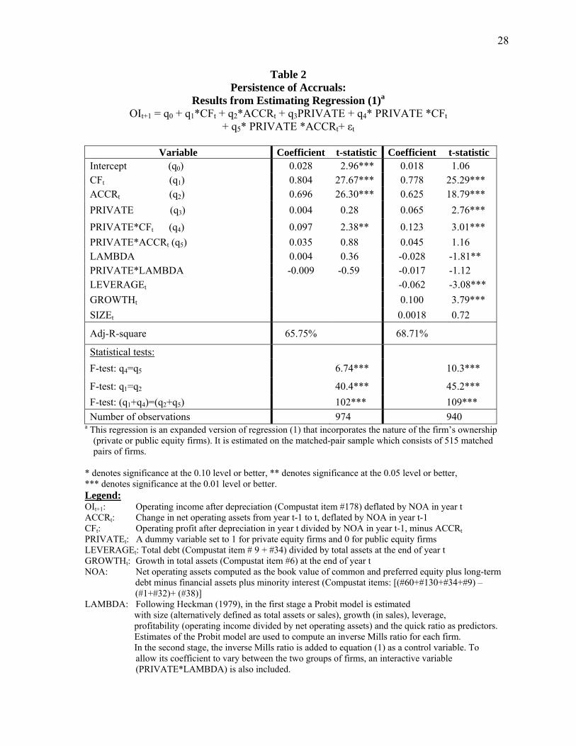
The results are presented in table 2. The table shows the coefficients of estimating an

expanded version of regression (1) that includes a dummy variable for the firm type (private

equity or public equity) and three control variables, leverage, growth and firm size. The high

level of significance of virtually all of the cash flow and accrual coefficients as well as the

relatively high explanatory of the regression suggest that it captures well the relation between

cash flows and accruals in the current year, and the operating income in the following year, for

both groups of firms.

The coefficients of interest are those on the cash flow and accrual components of

operating income as well as the difference in these coefficients between the private equity and

public equity firms. If the accrual component of earnings causes earnings to be relatively less

persistent than the cash flow component of earnings, then the coefficients on the accrual

components of earnings will be smaller than the coefficient on the cash flow component of

earnings. Using an F-test to test the equality of these coefficients (that is, q1=q2 for public equity

firms and (q1+q4) = (q2+q5) for private equity firms), the hypothesis that they are equal is rejected

for both types of firms in both the original and the augmented regression.

More important for our hypotheses, note that private equity firms exhibit a greater

persistence of both cash flows and accruals than do public equity firms. The incremental

coefficient of cash flows (q4) is positive and significant for both the original and the augmented

regression. The incremental coefficient of accruals (q5), while positive for both regressions, is

not statistically significant. Our conclusion is that the quality of earnings of private equity firms,

as captured by earnings persistence, is at least on par with, if not better than that of, public equity

18 See section 4.1 for a detailed description of this procedure. To obtain more efficient estimates for the cash flow and accrual variables, we also estimate regression (1) augmented by a number of variables that are likely to relate to future profitability (i.e., leverage, sales growth and firm size).

16

firms. This is consistent with the “opportunistic behavior” hypothesis which suggests that

financial reporting by public equity firms, because of capital market and managerial

compensation incentives, is more susceptible to management intervention.

6.3. Estimation error in the accrual process

The estimation error in the accrual process is gauged by the variability of the accruals

that remain unexplained by regression (2). The results from estimating this regression are

provided in table 3. The first line of the table shows the standard deviation of the regression

residuals as well as the ratio of that standard deviation to the standard deviation of the total

current accruals (the dependent variable).19 Note that both measures of variability are

significantly higher for public equity firms as compared with private equity firms. This is also

true for the industry analysis. In19 of the 23 industries that had a sufficient number (at least 20)

of both public equity and private equity companies, the standard deviation of the residuals from

regression (2) (the unexplained accrual variability) is higher for the public equity firms than for

those with private equity. In 20 of the industries, the ratio of the standard deviation of the

residuals from regression (2) to the standard deviation of total current accruals is higher for

public equity firms than for the private equity firms.

We also examine the hypothesis that the difference in the variability of unexplained

accruals is not higher for the public equity firms. The hypothesis is rejected at the 1%

significance level in favor of the alternative that public equity firms exhibit higher variability.

Public equity firms also exhibit significantly greater relative accrual variability (that is a higher

ratio of the standard deviation of residuals from regression (3) to that of total current accruals)

than their privately- owned peers operating in the same industries.

Based on these results, we conclude that the accrual estimation of public equity firms is

of a lower quality than that of private equity firms. This is consistent with our earlier findings on

the persistence of accruals, lending further support to the “opportunistic behavior” hypothesis.

6.4. Absence of earnings management

As explained in section 4.3, we identify the presence of earnings management in the two

groups of firms using two tests. The first is based on the distributional properties of earnings

around two earnings thresholds: zero earnings and zero earnings growth. We refer to this test as

19 The R2 values of regression (2) (not tabulated) when estimated separately for the public equity and the private equity firm-years are 49.9% and 41.5%, respectively.

17

the “threshold analysis.” The second test is based on the sign and magnitude of unexpected

accruals of those observations that fall just above the two earnings thresholds.

The results of the threshold analysis based on the matched-pair sample are presented in

Table 4. The table provides the actual and expected frequency of cases in the intervals “just

above” and “just below” the two earnings thresholds. The intervals are defined according to the

procedure suggested by DeGeorge et al. (1999). The results in the table pertain to an earnings

threshold where earnings are defined as income from continuing operations.20

Panels A and B of table 4 indicated that for both types of firms, the actual frequency of

cases just below (just above) the zero threshold of both earnings levels and earnings changes is

lower (higher) than the expected frequency for that interval. The standardized difference between

the expected and actual frequency, which under the null hypothesis will be distributed

approximately Normal(0,1), is statistically significant for most of the “just-above” regions. This

finding, which is comparable with previous findings (e.g., Burgstahler and Dichev (1997)), is

consistent with upward earnings management in cases that otherwise would have fallen slightly

short of the earnings thresholds.21

While the shift from the “just below” to the “just above” intervals is also present among

private equity firms, it is much less associated with positive earnings accruals as indicated by the

results reported in table 5. These results show the difference in the propensity to manage

earnings between public equity and private equity firms based on the proportion of positive

unexpected accruals among the just above zero cases. To more precisely pinpoint earnings

management cases, we examine the percentage of the positive unexpected accruals cases where

these accruals “made the difference,” that is their magnitude was sufficiently positive so as to

turn what would have otherwise been a loss into a small profit. The table, which is based on an

analysis of the matched-pair sample, shows the proportion of positive unexpected accruals for

the intervals just above the zero threshold. It also shows the proportion of cases in the just above

zero interval whose positive unexpected accruals were large enough to convert a loss into a small

20 While this definition most likely corresponds to the threshold that investors and management emphasize, we repeated the threshold analysis using bottom-line net income (i.e., net income after extraordinary items and discontinued operations) and with operating income. The findings were essentially the same. 21 For the sake of comparability, our analysis uses the same bin sizes as prior research (e.g., Degeorge et al. (1999)). When we repeat the analysis reported in Table 4 using bin sizes that are twice as large, the results clearly indicate that public equity firms engage in more upward earnings management than do private equity firms.

18

gain (that is, the amount of unexpected positive accruals for these cases was larger than the

amount by which reported income exceeded the threshold).

Two main findings emerge from table 5. First, the percentage of cases with positive

unexpected accruals in the interval just above the threshold is considerably higher for the public

equity firms than for the private equity firms. The first line of results indicates that 61.0% of the

public equity observations classified as being in the just above zero interval of the earnings

distribution contain unexpected positive accruals while only 41.4% of the private equity firms in

this interval had unexpected positive accruals. This difference of 19.6%, as well as that

pertaining to the zero earnings change threshold shown in panel B of 19.7%, are both statistically

significant at the 0.01 level. The other finding is that among these cases with positive unexpected

accruals that fall in the just above range, the frequency of cases where unexpected accruals alone

explain the excess over the threshold is larger for public equity than for the private equity firms.

To illustrate, the magnitude of the unexpected accruals was sufficient to turn a loss into a profit

for 91.5% of the public equity observations whereas for 82.6% of the private equity firm

observations the positive unexpected accruals were the means by which the firm’s earnings

exceeded the threshold. This difference of 8.9% is statistically significant at the 0.10 level. The

comparable difference of 3.1%, shown in panel B, while positive is not significant.

Table 5 also presents the magnitude of unexpected accruals in the regions just above the

zero threshold. The means (and medians) of the public equity firms’ unexpected accruals are

significantly larger than that of the private equity firms. The mean unexpected accruals (deflated

by assets) for the small profits region is 2.03% for public equity firms and only 0.39% for private

equity firms. The difference of 1.64% is statistically significant. In the same vein, the mean

unexpected accruals for the region of small positive earning changes is 1.28% for public equity

firms but negative, -0.51%, for private equity firms.

The results in table 5 indicate that the behavior of unexpected accruals around the

earnings thresholds is consistent with earnings management for public equity firms but generally

does not indicate earnings management for the private equity firms.22 These results suggest that

earnings management is more pronounced for public equity firms than it is for private equity

firms, consistent with the “opportunistic behavior” hypothesis.

22 When we repeat the analysis of table 5 using different bin sizes or employing the full sample we obtain similar results concerning the percentage of cases with positive negative accruals in the interval “just-above” the zero threshold.

19

6.5. Conservatism

As explained in section 4.4, we consider two attributes of conservatism. One attribute is

the timeliness of loss versus gain recognition, referred to in the literature as “conditional

conservatism.” We employ the measure proposed by Basu (1997) and used by Ball and

Shivakumar (2005) to assess the extent of such conservatism in the two groups of firms.

Following Ball and Shivakumar (2005), we account for possible endogeneity. Under

conservative accounting, losses will be recognized more promptly and therefore will have lower

persistence over time while gains will be gradually recognized in earnings resulting in an

observed higher persistence of gains. The second measure of conservatism captures the “hidden

reserves” that accumulate on the balance sheet. It reflects the impact of applying conservative

accounting principles and is referred to as “unconditional conservatism.” We gauge the extent of

this aspect of conservatism using the measures proposed by Penman and Zhang (2002).

The results of estimating regression (3) which assesses the extent of “conditional

conservatism” are presented in table 6. The coefficients of interest in this regression are those

relating to the differential persistence of earnings declines versus earnings increases (a3 for

public equity firms and a3 + a7 for private equity firms) as well as the difference in this

differential between these two groups of firms (a7).

Two main results emerge from this analysis. First, and consistent with previous research,

financial reporting in general is conservative. Earnings increases are significantly more persistent

than earnings decreases for both groups of firms. Both a3 and a3+a7 are negative and statistically

significant for both definitions of the earnings variable (a3 of -0.542 and -0.538, and a3+ a7 of

-0.190 and -0.292, for the two earnings definitions, respectively). Second, the extent of

conservatism is greater for public equity firms as compared to that for private equity firms. The

coefficient a7, which indicates the excess persistence of earnings declines over earnings increases

for public equity firms, is positive (0.352 and 0.246 for the two earnings definitions) and

statistically significant. The coefficient of the inverse Mills’ variable (Lambda) is significant for

both types of firms, suggesting the presence, and the appropriateness of controlling for,

endogeneity.

These results are consistent with those reported by Ball and Shivakumar (2005) for

private and public companies in the United Kingdom. Similar to that study, we interpret this

finding as indicating that public equity firms, because of the demand by investors and debt

20

holders, report more conservatively than do private equity firms in the sense of a more

pronounced earlier recognition of losses relative to gains. This finding of more conservative

reporting by public equity firms is consistent with the “demand” hypothesis.

The results concerning unconditional conservatism, captured by the Penman and Zhang

(2002) measures, are shown in table 7. The findings indicate that public equity firms display a

greater degree of unconditional conservatism. The accumulation on the balance sheet of “hidden

reserves” due to the combined effect of capitalizing R&D and advertising costs and using LIFO

for inventory valuation (the LIFO reserve) as a percentage of total net operating assets (the C-

Score) reaches 11.0% for public equity firms but only 6.8% for private firms.

The magnitude of these three reserves depends to a large extent on the industry in which

the firm operates. The need to control for industry exists even though, as noted earlier, there is

little difference in the industry distributions of public equity and private equity firms (see table

1). We control for the industry effect by comparing the Q-scores of the two groups of firms as

proposed by Penman and Zhang. The Q-score is computed by subtracting from each individual

firm’s cumulative reserve the median C-score in the firm’s 2-digit industry. The industry-

adjusted measures show similar results. That is, the “hidden reserves” loom larger on the balance

sheets of public equity firms than on those of their industry peers. The median accumulation of

the “hidden reserves” as a percentage of net operating assets for private equity firms is 2.2%

below their industry peers while that accumulation by public equity firms is 0.2% above their

industry peers. This difference of 2.4% is statistically significant (at the 0.01 level) and

consistent with the “opportunistic behavior” hypothesis.

7. Concluding Remarks

The findings of the paper illustrate that managerial incentives and investors’ demand for

earnings quality are important factors that shape the financial reporting of firms. Public

ownership in the firm’s equity exposes management to investors’ demand for reporting quality.

This demand, which is expressed by investors in the form of the regulatory and legal

environment in which the public equity firm operates, leads to higher reporting quality (the

“demand” hypothesis). At the same time, the findings support the notion that management of

firms whose equity is publicly traded have stronger incentives to manage earnings (in part due to

their stake in the publicly-traded stock), thus reducing the reliability and usefulness of financial

21

reporting (the “opportunistic behavior” hypothesis). Unless weights are assigned to different

dimensions of earnings quality, one cannot conclude that the public listing of a firm’s equity

necessarily improves the quality of its financial reporting.

An interesting question not addressed by this paper is the effect of debt and, in particular,

public debt, on earnings quality. Both groups of firms contrasted and analyzed in this paper have

public debt outstanding. The demand for accounting quality and the influence of management

incentives is likely to be different depending on whether the firm has debt or not and whether the

debt is private or public. Given the heavy reliance of creditors on financial statements for

contracting and monitoring and the importance of debt financing for corporations, the study of

this question, in which we are currently engaged, would further enhance our understanding of the

factors that affect earnings quality.

22

References

Ball, R., S.P. Kothari and A. Robin, 2000, “The Effect of International Institutional Factors on Properties of Accounting Earnings,” Journal of Accounting and Economics, v. 29 (1), pp. 1-51. Ball R., A. Robin and J.S. Wu, 2003, “Incentive versus Standards: Properties of Accounting Income in Four East Asian Countries,” Journal of Accounting and Economics, v. 30 (1-3), pp. 235-270. Ball R. and L. Shivakumar, 2005, “Earnings Quality in U.K. Private Firms: Comparative Loss Recognition Timeliness,” Journal of Accounting and Economics, v. 39(1), pp. 83-128. Barth M., J. Elliott and M. Finn, 1999, “Market Rewards Associated with Patterns of Increasing Earnings,” Journal of Accounting Research, v. 37 (2), pp. 387-413. Basu, S., 1997, “The Conservatism Principle and the Asymmetric Timeliness of Earnings,” Journal of Accounting and Economics, v. 24 (1), pp. 3-37. Berlin, M. and J. Loyes, 1988, “Bond Covenants and Delegated Monitoring,” Journal of Finance, v. 43(2), pp. 397-412. Bartov, E., D. Givoly and C. Hayn, 2002, “The Rewards to Meeting or Beating Earnings Expectations,” Journal of Accounting and Economics, v. 33 (2), pp.173-204. Boyd, J. and E. C. Prescott, 1986, “Financial Intermediary-Coalitions,” Journal of Financial Theory, v. 38(2), pp. 211-232. Burgstahler, D. and I. Dichev, 1997, “Earnings Management to Avoid Earnings Decreases and Losses,” Journal of Accounting and Economics, v. 24(1), pp. 99-126. Burgstahler D., H. Luzi and C. Leuz, 2006, “The Importance of Reporting Incentives: Earnings Management in European Private and Public Firms,” The Accounting Review, v. 81 (5), pp. 983-1016. Bushman R.M. and J.D Piotroski, 2004, “Financial Incentives for Conservative Accounting: The Influence of Legal and Political Institutions,” Journal of Accounting and Economics Conference. Campbell, S., 1979, “Optimal Investment Financing Decisions and the Value of Confidentiality,” Journal of Financial and Quantitative Analysis, v. 14(5), pp. 913-924. Cantillo, M., and J. Wright, 2000, “How Do Firms Choose their Lenders? An Empirical Investigation,” Review of Financial Studies v. 13(1), pp. 155-189. Carey, M., S. Prowse, J. Rea, and G. Udell, 1993, “The Economics of Private Placement Market,” Board of Governors of the Federal Reserve System: Washington DC.

23

Chemmanur, T. and P. Fulghieri, 1994, “Reputation, Renegotiation, and the Choice between Bank Loans and Publicly Traded Debt,” Review of Financial Studies, v. 7(3), pp. 475-506. Cohan, A. C., 1967, “Yields on Corporate Debt Directly Placed,” National Bureau of Economic Research, New York. Denis, D., and V. Mihov, 2003, “The Choice among Bank Debt, Non-Bank Private Debt and Public Debt: Evidence from New Corporate Borrowings”. Journal of Financial Economics, v. 70(1), pp. 3-28. Dechow, P. and I. Dichev, 2002, “The Quality of Accruals and Earnings: The Role of Accrual Estimation Errors”, The Accounting Review, v. 77 (Supplement), pp. 35-59. Dhaliwal, D. S., I. K. Khurana and R. Pereira, 2004, “Voluntary Disclosure and a Firm’s Decision to Issue Public versus Private Debt,” Working Paper, University of Arizona and University of Missouri – Columbia. Diamond, D. W., 1984, “Financial Intermediation and Delegated Monitoring,” Review of Economic Studies, v. 51(166), pp. 393-414. Fama, E., 1985, “What’s Different about Banks?” Journal of Monetary Economics, v.15(1), pp. 29-39. Francis, J., R. Z. LaFond, P. Olsson and K. Schipper, "Earnings Quality and the Pricing Effects of Earnings Patterns" (April 2003). (http://ssrn.com/abstract=414142) Francis, J., R. Z. LaFond, P. Olsson and K. Schipper, 2005, “The Market Pricing of Accruals Quality,” Journal of Accounting and Economics, v. 39 (2), pp. 295-327. Gertner, R. and D. Scharfstein, 1991, “A Theory of Workouts and the Effects of Reorganization Law,” Journal of Finance, v. 46(4), pp. 1189-1222. Givoly D., C. Hayn and A. Natarajan, 2007, “Measuring Reporting Conservatism,” The Accounting Review, v. 82 (1), pp. 65-106. Hayn, C., 1995, “The information content of losses,” Journal of Accounting and Economics, v. 20(2), pp. 125-153. Heckman, J.J., 1979. “Sample Selection Bias as a Specification Error,” Econometrica, v. 47(1), pp. 153-161. Houston, J. and C. James, 1996, “Bank Information Monopolies and the Mix of Private and Public Debt Claims,” Journal of Finance, v. 51(5), pp. 1863-1869. Hribar, P. and D. W. Collins, 2002, “Errors in Estimating Accruals: Implications for Empirical Research,” Journal of Accounting Research, v. 40 (1), pp. 105-134.

24

Johnson, S. A., 1997, “An Empirical Analysis of the Determinants of Corporate Debt Ownership Structure,” Journal of Financial and Quantitative Analysis, v. 32(1), pp.47-69. Kasznik, R. and B. Lev, 1995, “To Warn or Not to Warn: Management Disclosures in the Face of an Earnings Surprise,” The Accounting Review, v. 70(1), pp. 113-134. Krishnaswami, S., P. Spindt, and V. Subramaniam, 1999, “Information Asymmetry, Monitoring, and the Placement Structure of Corporate Debt,” Journal of Financial Economics, v. 51(3), pp. 407-434. Kwan S. and W. Carlton, 2003, “Financial Contracting and the Choice between Private Placement and Publicly Offered Bonds,” Working Paper, University of Arizona. McNichols, M., 2002. Discussion of “The Quality of Accruals and Earnings: The Role of Accrual Estimation Errors,” The Accounting Review, v. 77 (Supplement), pp. 61-69. Mikhail, M., B. Walther and R. Willis, 2003, “Reactions to Dividend Changes Conditional on Earnings Quality,” Journal of Accounting, Auditing & Finance, v. 18(1), pp.121-151.

Myers, S. C., 1984, “The Capital Structure Puzzle,” Journal of Finance, v. 39 (3), pp. 575-592.

Nissim, D. and S. H. Penman, 2003, “Financial Statement Analysis of Leverage and How It Informs about Profitability and Price-to-Book Ratios,” Review of Accounting Studies, v. 8(4), pp. 531-560.

Penman, S. H. and X. J. Zhang, 2002, "Accounting Conservatism, the Quality of Earnings, and Stock Returns," The Accounting Review, v. 77(2), pp. 237-264.

Penno, M., and Simon, D. T., 1986, “Accounting Choices: Public versus Private Firms,” Journal of Business Finance & Accounting, v. 86(13), pp. 561-570. Pope, P. and M. Walker, 1999, “International Differences in Timeliness, Conservatism and Classification of Earnings,” Journal of Accounting Research, v. 37 (Supplement), pp. 53-99. Richardson, S., A., R. G. Sloan, M. T. Soliman and A. I. Tuna, 2001, "Information in Accruals about the Quality of Earnings,” (July 2001). (http://ssrn.com/abstract=278308 ) Richardson, S., A., R. G. Sloan, M. T. Soliman and A. I. Tuna, 2005, "Accrual Reliability, Earnings Persistence and Stock Prices,” Journal of Accounting and Economics, v. 39 (3): pp. 437-485. Shi, C., 2002, “On the Trade-off between the Future Benefits and Riskiness of R&D: A Bondholders’ Perspective,” Journal of Accounting and Economics, v. 35 (2), pp. 227-254. Skinner, D. J., 1994, “Why Firms Voluntarily Disclose Bad News,” Journal of Accounting Research, v. 32(1), pp. 38-60.

25

Skinner, D. J., 1997, “Earnings Disclosures and Stockholder Lawsuits,” Journal of Accounting and Economics, v. 23(3), pp. 249-282. Sloan, R.G., 1996, “Do Stock Prices Fully Reflect Information in Accruals and Cash Flows about Future Earnings?” The Accounting Review, v. 71(3), pp. 289-315 Smith, C. W. and J. B. Warner, 1979, “On Financial Contracting: An Analysis of Bond Covenants,” Journal of Financial Economics, v. 7(2), pp. 117–161. Watts, R., 2003, “Conservatism in Accounting Part I: Explanations and Implications,” Accounting Horizons, v. 17 (3), pp. 207-221. Verdi, R. S., 2006, “Financial Reporting Quality and Investment Efficiency,” Working Paper, Sloan School of Management, MIT Yosha, O., 1995, “Information Disclosure Costs and the Choice of financing Source,” Journal of Financial Intermediation, v. 4(1), pp. 3-20.

26

Table 1 Descriptive Statistics on Private Equity and Public Equity Firmsa

Panel A: Owners of Private Equity Firmsb

Total Financial Sponsors Mgmt

Financial Sponsors

and Mgmt Employees

Unknown No. of Firms 531 292 119 81 17

32

No. of Firm-Year Obs. 2,519 1,203 613 348 186

169

a Both the private equity and public equity firms have publicly-traded debt. b Ownership of private equity firms was determined based on the majority ownership. Management ownership was based on the holdings of the founders, top executives, directors and family members. Employee ownership was based on the holdings of employees including their pension and stock option plans. The “unknown” category generally consists of firms with no available information regarding ownership. Panel B: Industry Affiliation of Private Equity and Public Equity Firmsa

Private Equity Firms Public Equity Firms Industry (two-digit SIC codes)

No. of Obs. % of

Sample No. of Obs. % of

Sample Mining & Construction (10-14, 15-17) 18 3.4 318 8.0Manufacturing I (20-29) 125 23.5 849 21.5Manufacturing II (30-39) 164 30.9 1439 36.4Transportation & Public Utilities(40-49) 21 4.0 158 4.0Retail & Wholesale Trade (50-59) 117 22.0 517 13.1Services (70-89) 84 15.8 628 15.9Other 2 0.4 45 1.1 Total Number of Firms

531 100% 3,954 100%

a Both private equity and public equity firms have publicly-traded debt.

27

Table 1 (continued) Descriptive Statistics on Private Equity and Public Equity Firms

Panel C: Financial Measures of Samplea

Public Equity Firms with:

Private Equity Firms with Public

Debt Public Debt Private Debt

No. of Firms 531 3,954 10,673No. of Firm-Year Observations 2,519 30,696 65,772Total Assets Mean 637 1,990 128(in $ millions) Median 337 483 39

Std.Dev. 845 4,188 249 Total Sales Mean 803 2,087 153 (in $ millions) Median 405 512 41

Std.Dev. 1,202 4,301 304Leverage Mean 67.2% 32.2% 25.5%(Total Debt/ Total Assets) Median 66.5% 29.5% 21.2%

Std.Dev. 31.1% 18.6% 21.9%Sales Growth Mean 5.6% 9.9% 15.3%

Median 4.6% 7.2% 8.5%Std.Dev. 14.1% 22.1% 39.9%

Return on Assets Mean 0.2% 3.2% -3.7%(Net Income / Total Assets) Median 0.9% 4.3% 2.4% Std.Dev. 8.0% 8.6% 21.6%

a The distribution of each variable is truncated at the extreme ±1% values. Panel D: Debt Rating for Private Equity and Public Equity Firmsa

Debt Rating Private Equity Firms Public Equity Firms

No. of Obs. % N %

BBB or Better 78 3.1 7,403 24.1BB 241 9.6 3,471 11.3B 1,001 39.7 2,890 9.4C – CCC 100 4.0 318 1.0D and Selective Default 9 0.4 187 0.6 Not Rated 1,090 43.3 16,427 53.5 Total number of firm-years

2,519 100% 30,696 100%

a Both private equity and public equity firms have publicly-traded debt.

28

Table 2 Persistence of Accruals:

Results from Estimating Regression (1)a OIt+1 = q0 + q1*CFt + q2*ACCRt + q3PRIVATE + q4* PRIVATE *CFt

+ q5* PRIVATE *ACCRt+ εt

Variable Coefficient t-statistic Coefficient t-statistic Intercept (q0) 0.028 2.96*** 0.018 1.06 CFt (q1) 0.804 27.67*** 0.778 25.29*** ACCRt (q2) 0.696 26.30*** 0.625 18.79*** PRIVATE (q3) 0.004 0.28 0.065 2.76*** PRIVATE*CFt (q4) 0.097 2.38** 0.123 3.01*** PRIVATE*ACCRt (q5) 0.035 0.88 0.045 1.16 LAMBDA 0.004 0.36 -0.028 -1.81** PRIVATE*LAMBDA -0.009 -0.59 -0.017 -1.12 LEVERAGEt -0.062 -3.08*** GROWTHt 0.100 3.79*** SIZEt 0.0018 0.72

Adj-R-square 65.75% 68.71%

Statistical tests: F-test: q4=q5 6.74*** 10.3***

F-test: q1=q2 40.4*** 45.2*** F-test: (q1+q4)=(q2+q5) 102*** 109*** Number of observations 974 940

a This regression is an expanded version of regression (1) that incorporates the nature of the firm’s ownership (private or public equity firms). It is estimated on the matched-pair sample which consists of 515 matched pairs of firms.

* denotes significance at the 0.10 level or better, ** denotes significance at the 0.05 level or better, *** denotes significance at the 0.01 level or better. Legend: OIt+1: Operating income after depreciation (Compustat item #178) deflated by NOA in year t ACCRt: Change in net operating assets from year t-1 to t, deflated by NOA in year t-1 CFt: Operating profit after depreciation in year t divided by NOA in year t-1, minus ACCRt PRIVATEt: A dummy variable set to 1 for private equity firms and 0 for public equity firms LEVERAGEt: Total debt (Compustat item # 9 + #34) divided by total assets at the end of year t GROWTHt: Growth in total assets (Compustat item #6) at the end of year t NOA: Net operating assets computed as the book value of common and preferred equity plus long-term

debt minus financial assets plus minority interest (Compustat items: [(#60+#130+#34+#9) – (#1+#32)+ (#38)]

LAMBDA: Following Heckman (1979), in the first stage a Probit model is estimated with size (alternatively defined as total assets or sales), growth (in sales), leverage, profitability (operating income divided by net operating assets) and the quick ratio as predictors. Estimates of the Probit model are used to compute an inverse Mills ratio for each firm. In the second stage, the inverse Mills ratio is added to equation (1) as a control variable. To

allow its coefficient to vary between the two groups of firms, an interactive variable (PRIVATE*LAMBDA) is also included.

29

Table 3 Estimation Error of the Accrual Process:

Variability and Relative Variability of the Residuals from Regression (2) TCAt = β0 +β1CFOt-1 + β2CFOt + β3CFOt+1 + β4ΔRevt + β5PPEt + εt

Public Equity Firms Private Equity Firms Industry

(2-digit SIC) No. of Obs.

[1] S.D. of

residuals

[2] Ratio of

S.D.

N [3] S.D. of

residuals

[4] Ratio of

S.D.

[5]=[1]-[3] Difference

in S.D.

[6]=[2]-[4] Difference in Ratio of

S.D.

All observations 13,527 4.17% 63.97% 843 2.90% 53.48%

1.27% ***

10.49% ***

22 306 4.23% 58.70% 26 1.52% 30.33% 2.70% 28.37% 23 272 5.27% 56.79% 27 3.49% 52.69% 1.78% 4.10% 25 294 3.61% 51.23% 22 4.41% 70.89% -0.79% -19.66% 27 508 4.09% 65.98% 41 1.46% 52.79% 2.63% 13.19% 28 1878 4.34% 74.56% 61 3.42% 77.21% 0.92% -2.64% 30 496 3.84% 64.70% 25 3.45% 49.76% 0.39% 14.94% 33 855 3.86% 65.59% 24 2.94% 49.77% 0.91% 15.82% 34 627 4.48% 63.15% 39 2.75% 47.02% 1.73% 16.13% 35 1716 5.21% 68.52% 43 3.13% 48.31% 2.07% 20.21% 36 1710 5.24% 66.10% 27 3.42% 51.42% 1.82% 14.68% 37 951 4.20% 61.58% 59 4.31% 69.73% -0.11% -8.15% 42 170 2.50% 59.96% 36 1.89% 37.39% 0.61% 22.58% 47 46 3.34% 56.32% 23 0.70% 44.58% 2.65% 11.74% 50 658 4.82% 54.31% 54 3.18% 50.25% 1.64% 4.06% 51 392 4.03% 50.62% 27 2.51% 28.13% 1.52% 22.49% 53 383 3.88% 57.36% 20 3.28% 46.54% 0.59% 10.82% 54 312 2.80% 73.52% 60 2.36% 67.27% 0.44% 6.25% 58 286 3.56% 72.25% 65 3.99% 69.88% -0.42% 2.37% 59 414 5.30% 72.17% 27 1.90% 38.31% 3.40% 33.86% 70 135 2.53% 63.10% 24 3.09% 81.67% -0.56% -18.57% 73 651 5.87% 78.26% 34 2.92% 52.46% 2.94% 25.79% 79 298 3.27% 71.01% 30 1.88% 48.46% 1.39% 22.55% 87 169 5.58% 65.65% 49 4.71% 65.20% 0.87% 0.44%

*** Significant at the 0.01 level; significance is determined using an F-test for equality of variances. Legend: TCAt: Total current accruals calculated as ΔCA-ΔCL-ΔCash+ΔSTDEBT where changes are computed from year

t-1 to year t and CA refers to current assets, CL refers to current liabilities and STDEBT is the current portion of long-term debt.

CFOt: Cash flow from operations computed as income from continuing operations in year t minus total accruals in year t (total accruals in year t equal TCAt – depreciation and amortization in year t).

ΔRevt: Change in revenues from year t-1 to year t. PPEt: PPE (gross) in year t.

30

Table 4

Frequency Distribution of Earnings around the Zero-Earnings and Zero-Earnings-Growth Thresholds

(for the Matched-Pairs Sample)

Panel A: Zero-Earnings Thresholda

Public Equity Firms (n=799 firms years)

Private Equity Firms

(n=799 firm years)

Frequency of Observations

Frequency of Observations

Intervalb

Actual Expectedc

Std.

Differenced Actual Expected

Std.

Difference

“Just below zero” 37 60.5 -2.66 91 99.5 -0.78

“Just above zero” 79 72.0 0.72 111 90.5 1.89

Panel B: Zero Earnings Growth Thresholda

Public Equity Firms (n=542 firms years)

Private Equity Firms

(n=542 firm years)

Frequency of Observations

Frequency of Observations

Interval

Actual Expected

Std.

Difference Actual Expected

Std.

Difference

“Just below zero” 64 73.0 -0.98 65 71 -0.66

“Just above zero” 97 63.5 3.68 98 61 4.13

a In Panel A, the distribution of income from continuing operations in year t divided by total assets at the end of year t-1 (Income/ Total Assets) is examined in order to assess potential earnings management around this threshold. In Panel B, the distribution of the change in income from continuing operations from year t-1 to year t divided by total assets at the end of year t-2 (ΔIncome /Assets) is examined.

b Following Degeorge et al. (1999), to determine the number of observations “just above” and “just below” zero, a bin width, BW, is defined as follows: BW = 2(IQR)n-1/3, where IQR is the sample inter-quartile range and n is the number of observations. Based on this formula, the bin width applied is 0.016 for the distribution of Income /Assets as shown in panel A and 0.011 for the distribution of ΔIncome /Assets shown in Panel B.

c The expected frequency in the interval is computed as the average of the number of observations in the two adjacent intervals.

d The standardized difference is the difference between the actual and expected frequency in the interval, divided by the standard deviation of the difference. The standard deviation of the difference is computed according to Burgstahler and Dichev (1997) as the square root of [N*Pi*(1 – Pi) + (1/4)*N*(Pi-1 + Pi+1)(1 - Pi-1 - Pi+1)], where N is the total number of observations and Pi is the probability that an observation will fall into interval i.

31

Table 5 Unexpected Accruals Behavior in the “Just Above Zero” Intervala

(for the Matched Pairs Sample) Panel A: Zero Earnings Threshold (n=763 matched pairs)b

Percentage of Observationsc

Cases with: Public Equity Firms

Private Equity Firms

Difference in

Percentage of

Observations

Frequency of Cases with Positive Unexpected Accrualsc

(Out of all cases in the interval; no. of observations equals 77 and 111 for public equity and private equity firms, respectively)

61.0%

41.4% 19.6%***

Frequency of Cases with Positive Unexpected Accruals Larger that the Excess over the Thresholdd

(Out of all cases in the interval that have positive unexpected accruals)

91.5% 82.6% 8.9%*

Mean (median) unexpected accruals 2.03% (1.34%)

0.39% (-0.58%)

1.64%* (1.92%**)

Panel B: Zero Earnings Growth Threshold (n=524 matched pairs)

Frequency of Cases with Positive Unexpected Accrualsc

(Out of all cases in the interval; no. of observations equals 94 and 93 for public equity and private equity firms, respectively)

63.8% 44.1% 19.7%***

Frequency of Cases with Positive Unexpected Accruals Larger that the Excess over the Thresholdd

(Out of all cases in the interval that have positive unexpected accruals)

93.3% 90.2% 3.1%

Mean (median) unexpected accruals 1.28% (1.69%)

-0.51% (-0.93%)

1.79%* (2.62%***)

* denotes significance at the 0.10 level or better, ** denotes significance at the 0.05 level or better, *** denotes significance at the 0.01 level or better. Statistical significance is assessed using the t-test for differences in proportions. a The interval just above (just below) zero is defined as the first positive (first negative) “bin” of the distribution. The bin

widths are 0.016 and 0.011 for the distributions of Income/Total Assets and ΔIncome /Assets, respectively. Bin widths (BW) are determined by the formula: BW = 2(IQR)n-1/3, where IQR is the sample inter-quartile range and n is the number of observations.

b In Panel A, the distribution of income from continuing operations in year t divided by total assets at the end of year t-1 (Income/ Total Assets) is examined in order to assess potential earnings management around this threshold. In Panel B, the distribution of the change in income from continuing operations in from year t-1 to year t divided by total assets at the end of year t-2 (ΔIncome /Assets) is examined.

c Unexpected accruals are derived from the cross-sectional Jones model (see section 4.3). d Cases where the threshold would not have been met in the absence of positive unexpected accruals.

32

Table 6 Differential Persistence of Profits versus Losses by Firm Type

Summary Results for Expanded Version of Regression (3): ΔNIt = a0 + a1*DΔNIt -1 + a2*ΔNIt -1 + a3*DΔNIt -1*ΔNIt –1 + a4*PRIVATE + a5*PRIVATE*DΔNIt -1 +

a6*PRIVATE*ΔNIt -1 + a7*PRIVATE*DΔNIt-1*ΔNIt -1 + et

Earnings Measure

Net Income Income from Continuing Operations Variablea

Predicted Sign under

Conservatism and the

“Demand” Hypothesis Coefficient t-statistic Coefficient t-statistic

Intercept (a0) ? 0.004 4.63*** 0.003 4.35***DΔNIt –1 (a1) ? -0.011 -8.96*** -0.009 -8.56***ΔNIt –1 (a2) 0 -0.068 -5.41*** 0.003 0.25DΔNIt -1*ΔNIt –1 (a3) - -0.542 -28.64*** -0.538 -28.2***PRIVATE (a4) ? -0.022 -4.91*** -0.023 -5.60***PRIVATE*DΔNIt –1 (a5) ? -0.004 -1.57 0.002 0.85PRIVATE*ΔNIt –1 (a6) - -0.237 -9.65*** -0.176 -5.50***PRIVATE*DΔNIt-1*ΔNI t –1 (a7) + 0.352 9.17*** 0.246 4.87*** a3+ a7 (F-test)b - -0.190 5.73*** -0.292 11.24*** LAMBDA (a8) 0.081 21.25*** 0.064 19.86***PRIVATE*LAMBDA (a9) -0.067 -18.72*** -0.051 -15.9*** Adj-R-square 10.83% 8.13% No. of Observations 22,439 22,362

*significant at the 0.01 level or better; ** significant at the 0.05 level or better; ***significant at the 0.01 level or better

aEach variable in the table is truncated at the extreme +/-1% values of their distribution. bThe F-test is used to test the hypothesis that a3+ a7 = 0. Legend: ΔNIt: the change in the earnings measure from year t-1 to year t, standardized by total assets at the end

of year t-1. DΔNI: a dummy variable which is set to 1 if ΔNIt -1 < 0 and 0 otherwise. PRIVATE: a dummy variable that is set to 1 for private equity firms and 0 for public equity firms. LAMBDA: see the description provided in Table 2.

33

Table 7 Magnitude of Off-Balance-Sheet “Hidden Reserves”

“Hidden Reserves” as a Percentage of Net Operating Assetsa

Capitalized R&D

LIFO Reserve Capitalized Advertising

Total Reserves

(C-Score b)

Industry Adjusted Level of Reserves

(Q-Scorec)

Panel A: Public Equity Firms (n=3,954 firms; 30,696 firm-year observations)

Mean 7.5% 6.6% 6.5% 11.0% 4.1% Median 3.4% 4.1% 3.4% 6.6% 0.2%

% Positive 98.5% 98.1% 98.4% 98.4% 51.3% No. of obs. 14,559 10,397 11,032 22,699 22,699

Panel B: Private Equity Firms (n=531 firms; 2519 firm-year observations)

Mean 2.7% 5.4% 6.7% 6.8% 0.4% Median 1.2% 1.7% 3.5% 3.4% -2.2%

% Positive 100.0% 91.9% 98.5% 97.5% 31.4% No. of obs. 672 580 909 1,625 1,625

Difference in:d

Mean Values 4.8%*** 1.2%** -0.1% 4.2%*** 3.8%*** Median Values 2.2%*** 2.4%*** -0.04%*** 3.3%*** 2.4%***

*significant at the 0.10 level or better; ** significant at the 0.05 level or better; ***significant at the 0.01 level or better

a Each variable in the table is truncated at the extreme +/-1% values of their distribution. b The C-Score is a conservatism index that measures the extent of “hidden reserves” on the balance sheet. It is

computed as (INVtres + RDt

res + ADVtres) / NOAt-1, where INVres is the LIFO reserve, RDres and ADVres are the

estimated values of the R&D and advertising assets that would have been reported had these costs not been expensed. The R&D asset is estimated by “capitalizing” the annual R&D expenditure and amortizing it using the sum-of-the-years’ digits method over five years. The ADV asset is estimated using a similar approach and employing a two-year amortization period. NOA is the net operating assets, calculated as the book value of common and preferred equity plus total debt minus financial assets (defined as the sum of cash, short-term investments, and investments and advances) plus minority interest.

c The Q-Score is a conservatism measure equal to the firm’s C-Score minus the median C-Score in the firm’s industry.

d Differences in means are tested for significance using a two-tailed t-test; differences in medians are tested for significance using a two-tailed Wilcoxon signed rank test.