arX

iv:a

stro

-ph/

0207

608v

1 2

9 Ju

l 200

2

Do Neutron Star Gravitational Waves Carry Superfluid Imprints?

G. L. Comer

Department of Physics, Saint Louis University, St. Louis, MO, 63156-0907, USA

Isolated neutron stars undergoing non-radial oscillations are expected to emit grav-

itational waves in the kilohertz frequency range. To date, radio astronomers have

located about 1,300 pulsars, and can estimate that there are about 2 × 108 neutron

stars in the galaxy. Many of these are surely old and cold enough that their in-

teriors will contain matter in the superfluid or superconducting state. In fact, the

so-called glitch phenomenon in pulsars (a sudden spin-up of the pulsar’s crust) is

best described by assuming the presence of superfluid neutrons and superconducting

protons in the inner crusts and cores of the pulsars. Recently there has been much

progress on modelling the dynamics of superfluid neutron stars in both the Newto-

nian and general relativistic regimes. We will discuss some of the main results of

this recent work, perhaps the most important being that superfluidity should affect

the gravitational waves from neutron stars (emitted, for instance, during a glitch)

by modifying both the rotational properties of the background star and the modes

of oscillation of the perturbed configuration. Finally, we present an analysis of the

so-called zero-frequency subspace (i.e. the space of time-independent perturbations)

and determine that it is spanned by two sets of polar (or spheroidal) and two sets of

axial (or toroidal) degenerate perturbations for the general relativistic system. As in

the Newtonian case, the polar perturbations are the g-modes which are missing from

the pulsation spectrum of a non-rotating configuration, and the axial perturbations

should lead to two sets of r-modes when the degeneracy of the frequencies is broken

by having the background rotate.

I. INTRODUCTION

Jacob Bekenstein is one of those rare individuals who can make significant, original con-

tributions to diverse areas of theoretical physics. He is also a man of great integrity and, I

2

believe, has a humility that serves him well in advising and supporting students and young

scientists. I am profoundly grateful that fate allowed me to be one of those young scientists

and now lets me participate in this celebration of his career. One of the areas of theoret-

ical physics that Jacob has worked on is relativistic fluid dynamics. This is an important

component of my current area of research, which is to develop models of Newtonian and

general relativistic superfluid neutron stars. My original interest in superfluids, appropri-

ately enough, was sparked by Jacob, when he suggested that I look at superfluid analogs of

effects predicted for quantum fields in curved spacetimes (the Hawking and Fulling-Davies-

Unruh effects). My current interest in superfluids is to determine how the dynamics of

superfluid neutron stars differ from their ordinary, or perfect, fluid counterparts and if the

different dynamics can lead to observable effects in gravitational waves. In the remainder

of this article, I will give an overview of what my collaborators and I have accomplished

so far, including some new results (from work with Nils Andersson) on the structure of the

so-called zero-frequency subspace (i.e. the space of time-independent perturbations). The

main purpose is to show that superfluidity in neutron stars should affect their gravitational

waves in two ways, by modifying the rotational properties of the background star and the

modes of oscillation of the perturbed configuration.

While there are many mysteries about neutron stars that remain to be explained, we do

have some significant observational facts to work with. For instance, Lorimer [1] reports that

nearly 1300 pulsars (i.e. rotating neutron stars) have now been observed. By extrapolating

the data on the local population, he can estimate that there are about 1.6 × 105 normal

pulsars and around 4 × 104 millisecond pulsars in our galaxy. Of course, there are also

neutron stars that are no longer active pulsars. To get a handle on their number Lorimer

takes the observed supernova rate, which is about 1 per 60 years, and the age of the universe

to find about 2 × 108 neutron stars in the galaxy. The overwhelming majority of these

objects must be very cold in the sense that their (local) temperatures are much less than

the (local) Fermi temperatures of the independent species of the matter. One can estimate

the Fermi temperature to be about 1012 K for neutrons at supra-nuclear densities, and it is

generally accepted that within the first year (and probably much sooner than that) nascent

neutron stars should cool to temperatures less than 109 K. This is an interesting fact, in

that nuclear physics calculations of the transition temperature for neutrons and protons

to become superfluid and superconducting, respectively, consistently yield a value that is

3

109 K in order of magnitude (for recent reviews see [2, 3]). Thus we can expect that a

significant portion of the neutron stars in our galaxy will have at least two (and perhaps

more) superfluids in their cores.

In addition to nuclear physics theory and experiment, the well-established glitch phe-

nomenon in pulsars (e.g. Vela and Crab) [4, 5] is perhaps the best piece of evidence that

supports the existence of superfluids in neutron stars. A glitch is a sudden spin-up of the

observed rotation rate of a neutron star, and can have a relaxation time of weeks to months

[6]. Baym et al [7] have noted that a relaxation mechanism based on ordinary fluid viscosity

would be much too short to explain a weeks to months timescale and so they argue that this

signals the presence of a neutron superfluid. Now, a mainstay idea for explaining glitches is

that of superfluids and their vortex dynamics, i.e. how the vortices get pinned, unpinned,

and then repinned [8, 9, 10] to nuclei in the inner crusts of the glitching pulsars. This is

known as the vortex creep model and in it glitches are a transfer of momentum via vortices

from one angular momentum carrying component of the star to another. The model has

worked well to describe both the giant glitches in Vela and the smaller ones of the Crab. The

vortex creep model can also be used to infer the internal temperature of a glitching pulsar,

and for Vela it implies a temperature of 107 K [10]. It is also interesting to note the work of

Tsakadze and Tsakedze [11] who have experimented with rotating superfluid Helium II and

find behaviour very much like glitches in pulsars.

The classic description of superconductivity in ordinary condensed matter systems is

based on the so-called “BCS” mechanism (see, for instance, [12] or [13] for excellent presen-

tations): the particles that become superconducting must be fermions, and below a certain

transition temperature there must be an (usually effective) attractive interaction between

them (at the Fermi surface with zero total momentum). The interaction leads to so-called

Cooper-pairing where a pair of fermions act like a single boson and a collection of them

can behave as a condensate. The mechanism is very robust, which is why it also forms

the basis for discussion of nucleon superfluidity and superconductivity [14]; i.e. nucleons are

fermions and the effective interaction between them at nuclear and supra-nuclear densities

can be attractive. For instance, it is known experimentally that the lowest excited states

in even-even nuclei are systematically higher than other nuclei because of pairing between

nucleons which must be broken [12].

After many years of development, beginning with the work of Migdal [15], a consistent

4

picture has emerged (in part, from gap calculations [2, 3]): At long-range the nuclear force

is attractive and leads to neutron “Cooper” pairing in 1S0 states in the inner crust, but

because of short-range repulsion in the nuclear force and the spin-orbit interaction neutrons

pair into 3P2 states in the more dense regions of the core [16]. In the crust protons are locked

inside of neutron rich nuclei embedded in a degenerate normal fluid of electrons. In the inner

crust the nuclei are also embedded in, and even penetrated by, the superfluid neutrons. In

the core, however, the nuclei have dissolved and the protons remain dilute enough that they

feel only the long-range attractive part of the nuclear force and pair in 1S0 states. There is

no pairing between neutrons and protons anywhere in the core since their respective Fermi

energies are so different. The core superfluid neutrons and superconducting protons are also

embedded in a highly degenerate normal fluid of electrons. Other possibilities, such as pion

or hyperon condenstates, have been put forward but we will keep to the simplest scenario

that considers only superfluid neutrons, superconducting protons, crust nuclei, and normal

fluid electrons.

There are several ways in which the dynamics of a superfluid differ from its ordinary

fluid counterpart, and each difference should have some impact on the gravitational waves

that a superfluid neutron star emits. One key difference is that a pure superfluid is locally

irrotational. A superfluid, however, can mimic closely ordinary fluid rotation by forming a

dense array of (quantized) vortices. In the core of each vortex the superfluidity is destroyed

and the particles are in an ordinary fluid state, and can carry non-zero vorticity. A sec-

ond, very important difference is when there are several species of matter in a superfluid,

or superconducting, state. The superfluids of all the species will interpenetrate and each

superfluid will be dynamically independent having its own unit four-vector and local particle

number density. Lastly, superfluids have zero viscosity, but when vortices and excitations

are present, then dissipative mechanisms can exist. For instance, the scattering of excita-

tions off of the normal fluid in the vortex cores can lead to dissipative momentum exchange

between the excitations and the superfluid, the net effect being that the superfluid motion

becomes dissipative. This form of dissipative mechanism is known as mutual friction.

In neutron stars there is a very efficient form of mutual friction [14, 17, 18] that depends

on the entrainment effect [19, 20], which Sauls [14] describes as follows: even though the

neutrons are superfluid and the protons are superconducting both will still feel the long-

range attractive component of the nuclear force. In such a system of interacting fermions

5

the resulting excitations are quasiparticles. This means that the bare neutrons (or protons)

are “dressed” by a polarization cloud of nucleons comprised of both neutrons and protons.

Since both types of nucleon contribute to the cloud the momentum of the neutrons, say, is

modified so that it is a linear combination of the neutron and proton particle number density

currents. The same is true of the proton momentum. Thus when one of the nucleon fluids

starts to flow it will, through entrainment, induce a momentum in the other fluid. Alpar et al

[17] have shown that the electrons track very closely the superconducting protons (because

of electromagnetic attraction). Around each vortex is a flow of the superfluid neutrons.

Because of entrainment, a portion of the protons, and thus electrons too, will be pulled

along with the superfluid neutrons. The motion of the plasma leads to magnetic fields being

attached to the vortices. The mutual friction in this case is the dissipative scattering of the

normal fluid electrons off of the magnetic fields attached to the vortices.

There has been much effort put forward to develop Newtonian [21, 22, 23, 24, 25] and

general relativistic formalisms [26, 27, 28, 29, 30, 31, 32, 33, 34] for describing superfluid

neutron stars. In the simplest, but still physically interesting, formalism one has a system

that consists of two interpenetrating fluids—the superfluid neutrons in the inner crust and

core and the remaining charged constituents (i.e. crust nuclei, core protons, and crust and

core electrons) that will be loosely referred to as “protons”—and the entrainment effect

that acts between them. In principle the model can be expanded to have more than two

interpenetrating fluids (see [35] for instance). As well a given superfluid can be confined to

a distinct region in the star [36]. In this way the proton fluid, say, can be made to extend

out farther than the superfluid neutrons. This is a first approximation at incorporating the

fact that the superfluid neutrons do not extend all the way to the surface of the star.

Our primary goal is to show that superfluidity will affect gravitational wave emission from

neutron stars. We will see that a suitably advanced, but plausible, detector will have enough

sensitivity at high frequency to see modes excited during a glitch. With such detections we

will be able to place constraints, say, on the parameters that describe entrainment. But

in addition to studying glitches, we also need to analyze further the recently discovered

instability in the r-modes of neutron stars [37, 38]. The instability is driven by gravitational

wave emission (the CFS mechanism [39, 40, 41]) and the waves are potentially detectable by

LIGO II [42, 43, 44]. The conventional wisdom early on stated that mutual friction would

act against the instability in a superfluid neutron star and thus effectively suppress the

6

gravitational radiation. But Lindblom and Mendell [45] have found that mutual friction is

largely ineffective at suppressing the r-mode instability. However, there are many questions

about the spectrum of oscillation modes allowed by a rotating superfluid neutron star and

the analysis of instabilities is very likely to be much richer than the ordinary fluid case.

Thus, another goal here is to lay some groundwork for a future detailed study of the CFS

mechanism in superfluid neutron stars. Specifically, we will demonstrate that the zero

frequency subspace is spanned by two sets of polar (or spheroidal) and two sets of axial (or

toroidal) degenerate perturbations for the general relativistic system. Like the Newtonian

case [46], the polar perturbations are the g-modes which are missing from the pulsation

spectrum of a non-rotating configuration, and the axial perturbations should lead to two

sets of r-modes when the degeneracy of the frequencies is broken by having the background

rotate.

Below we will alternate between discussions based on Newtonian gravity and those us-

ing general relativity. Accuracy demands that a fully relativistic formalism be employed,

however there are some questions of principle for which a Newtonian formalism can suffice.

For instance, in determining the number of different modes of oscillation that a superfluid

neutron star can undergo it is much more tractable to use the Newtonian equations. But,

ulitmately there is the need for a general relativistic formalism. Newtonian gravity does not

include gravitational waves and so one needs a fully relativistic formalism to get an accurate

damping time of a mode of oscillation due to gravitational wave emission. Also, there is

the well-known problem that Newtonian models do not produce reliable values for the mass

and radius, in that, for a given central density, the predicted mass and radius in Newtonian

models may differ considerably from those of general relativity. This is a crucial point since

the superfluid phase transition in a neutron star is sensitive to density, as are the parameters

relevant to entrainment, and the oscillation frequencies can depend sensitively on mass and

radius.

II. GENERAL RELATIVISTIC AND NEWTONIAN SUPERFLUID

FORMALISMS

Based on the preceeding discussion, our formalism for modelling superfluid neutron stars

must allow for two interpenetrating fluids (i.e. the neutrons and “protons”) and the entrain-

7

ment effect. This must be the case whether we are working in the general relativistic regime

or the Newtonian limit. A general relativistic superfluid formalism has been developed by

Carter and Langlois [26, 27, 30, 31, 32] and their collaborators [28, 29, 33, 34]. Here an

action principle will be outlined that yields the equations of motion and the stress-energy

tensor for this system. Although a variational principle also exists for the Newtonian regime

[25], we will briefly indicate how to get the Newtonian equations by taking the appropri-

ate limit of the general relativistic equations (see [46] for full details). In the same spirit,

we will use a “slow” velocity approximation to motivate an expansion that can be used to

incorporate existing models of the entrainment effect [36].

A. The General Relativistic Formalism

In this subsection the equations of motion and stress-energy tensor for a two-component

general relativistic superfluid are obtained from an action principle. Specifically a so-called

“pull-back” approach (for instance, see [28, 29]) is used to construct Lagrangian displace-

ments of the number density four-currents that form the basis of the variations of the fluid

variables in the action principle (they will also be used later in the analysis of the zero-

frequency subspace). It will generalize to the superfluid case some of the techniques used to

analyze the CFS mechanism in ordinary fluid neutron stars [40, 41]. Finally, it can serve as

a starting point for generalizing the Hamiltonian formalism developed by Comer and Lan-

glois [29] who limited their discussion to a superfluid in the Landau state [12] (i.e. purely

irrotational).

For both the rotation and mode calculations effects such as “transfusion” [33] of one

component into the other (because of the weak interaction, for instance) will be ignored.

The neutron and proton number density four-currents, to be denoted nµ and pµ respectively,

are thus taken to be separately conserved, meaning

∇µnµ = 0 , ∇µp

µ = 0 . (1)

Such an approximation is reasonable for the mode calculations since the time-scale of the

oscillations (which is milliseconds) is much less than the weak interaction time-scale in

neutron stars, as long as the amplitudes of the oscillations remain small enough [47]. In

the case of slowly rotating neutron stars, it has been shown [48, 49] that when the neutrons

8

and protons rotate rigidly at different rates then chemical equilibrium cannot exist between

them. Of course, the energy associated with the relative rotation could be dissipated through

a process like transfusion. But Haensel [50] has demonstrated that such a process would take

months to years in mature neutron stars, and so again it will be neglected (since ultimately

we are interested in gravitational waves emitted during a glitch, say, the timescale of which

would be much shorter than the transfusion timescale).

By introducing the duals to nµ and pµ, i.e.

nνλτ = ǫνλτµnµ , nµ =

1

3!ǫµνλτnνλτ , (2)

and

pνλτ = ǫνλτµpµ , pµ =

1

3!ǫµνλτpνλτ , (3)

respectively, then the conservation rules are equivalent to having the two three-forms be

closed, i.e.

∇[µnνλτ ] = 0 , ∇[µpνλτ ] = 0 . (4)

The reason for introducing the duals is that it is straightforward to construct particle number

density three-forms that are automatically closed. The point is that the conservation of the

particle number density currents should not—speaking from a strict field theoretic point of

view—be a part of the system of equations of motion, rather they should be automatically

satisfied when the “true” system of equations is imposed.

This can be made to happen by introducing two three-dimensional abstract spaces which

can be labelled by coordinates XA and Y A, respectively, where A, B, C etc = 1, 2, 3. By

“pulling-back” each three-form onto its respective abstract space we can construct three-

forms that are automatically closed on spacetime, i.e. let

nνλτ = NABC(XD)∇νXA∇λX

B∇τXC , pνλτ = PABC(Y D)∇νY

A∇λYB∇τY

C (5)

where NABC and PABC are completely antisymmetric in their indices. Because the abstract

space indices are three-dimensional and the closure condition involves four spacetime indices,

and also that the XA and Y A are scalars on spacetime (and thus two covariant differentiations

commute), the pull-back construction does indeed produce a closed three-form:

∇[µnνλτ ] = ∇[µ

(

NABC(XD)∇νXA∇λX

B∇τ ]XC)

≡ 0 , (6)

9

and similarly for the protons. In terms of the scalar fields XA and Y A, we now have particle

number density currents that are automatically conserved, and so another way of viewing

the pull-back construction is that the fundamental fluid field variables are the spacetime

functions XA and Y A [51]. The variations of the three-forms can now be derived by varying

them with respect to XA and Y A.

Let us introduce two Lagrangian displacements on spacetime for the neutrons and pro-

tons, to be denoted ξµn and ξµ

p , respectively. These are related to the variations δXA and

δY A via a “push-forward” construction:

δXA = −(

∇µXA)

ξµn , δY A = −

(

∇µYA)

ξµp . (7)

Using the fact that

∇νδXA = −∇ν

([

∇µXA]

ξµn

)

= −(

∇µXA)

∇νξµn −

(

∇µ∇νXA)

ξµn , (8)

and similarly for the proton variation, then we find [33]

δnνλτ = − (ξσn∇σnνλτ + nσλτ∇νξ

σn + nνστ∇λξ

σn + nνλσ∇τξ

σn) = −Lξn

nνλτ ,

δpνλτ = −(

ξσp∇σpνλτ + pσλτ∇νξ

σp + pνστ∇λξ

σp + pνλσ∇τξ

σp

)

= −Lξppνλτ , (9)

where L is the Lie derivative. We can thus infer that

δnµ = nσ∇σξµn − ξσ

n∇σnµ − nµ(

∇σξσn +

1

2gσρδgσρ

)

,

δpµ = pσ∇σξµp − ξσ

p∇σpµ − pµ(

∇σξσp +

1

2gσρδgσρ

)

. (10)

By introducing the two decompositions

nµ = nuµ , uµuµ = −1 ,

pµ = pvµ , vµvµ = −1 , (11)

then we can show furthermore that

δn = −∇σ (nξσn) − n

(

uνuσ∇σξ

νn +

1

2[gσρ + uσuρ] δgσρ

)

,

10

δp = −∇σ

(

pξσp

)

− p(

vνvσ∇σξν

p +1

2[gσρ + vσvρ] δgσρ

)

, (12)

and

δuµ =(

δµρ + uµuρ

)

(uσ∇σξρn − ξσ

n∇σuρ) +

1

2uµuσuρδgσρ ,

δvµ =(

δµρ + vµvρ

) (

vσ∇σξρp − ξσ

p∇σvρ)

+1

2vµvσvρδgσρ . (13)

We will take one more step ahead and associate a notion of Lagrangian variation with

each Lagrangian displacement. These are defined to be

∆n ≡ δ + Lξn, ∆p ≡ δ + Lξp

, (14)

so that it now follows that

∆nnµλτ = 0 , ∆ppµλτ = 0 , (15)

which is entirely consistent with the pull-back construction. We also find that

∆nuµ =

1

2uµuσuρ∆ngσρ , ∆pv

µ =1

2vµvσvρ∆pgσρ , (16)

∆nǫνλτσ =1

2ǫνλτσg

µρ∆ngµρ , ∆pǫνλτσ =1

2ǫνλτσg

µρ∆pgµρ , (17)

and

∆nn = −n

2(gσρ + uσuρ) ∆ngσρ , ∆pp = −p

2(gσρ + vσvρ)∆pgσρ . (18)

However, in contrast to the ordinary fluid case [40, 41], there are many more options to

consider. For instance, we could also look at the Lagrangian variation of the neutron number

density with respect to the proton flow, i.e. ∆pn, or the Lagrangian variation of the proton

number density with respect to the neutron flow, i.e. ∆np. It is not clear at this point

how the existence of two preferred rest frames—one that is attached to the neutrons and

the other that is attached to the protons—will affect an analysis of the CFS mechanism in

superfluid neutron stars.

Nevertheless, with a general variation of the conserved four-currents in hand, we can now

use an action principle to derive the equations of motion and the stress-energy tensor. The

central quantity is the so-called “master” function Λ, which is a function of all the different

11

scalars that can be formed from nµ and pµ, i.e. the three scalars n2 = −nµnµ, p2 = −pµpµ,

and x2 = −pµnµ. In the limit where the two currents are parallel, i.e. the two fluids are

comoving, then the master function is such that −Λ corresponds to the local thermodynamic

energy density. In the action principle, the master function is the Lagrangian density for

the two fluids.

An unconstrained variation of Λ(n2, p2, x2) with respect to the independent vectors nµ

and pµ and the metric gµν takes the form

δΛ = µµδnµ + χµδp

µ +1

2(nµµν + pµχν) δgµν , (19)

where

µµ = Bnµ + Apµ , χµ = Cpµ + Anµ , (20)

and

A = − ∂Λ

∂x2, B = −2

∂Λ

∂n2, C = −2

∂Λ

∂p2. (21)

The momentum covectors µµ and χµ are dynamically, and thermodynamically, conjugate to

nµ and pµ, and their magnitudes are, respectively, the chemical potentials of the neutrons

and the protons. The two momentum covectors also show the entrainment effect since it is

seen explicitly that the momentum of one constituent carries along some mass current of

the other constituent (for example, µµ is a linear combination of nµ and pµ). We also see

that entrainment vanishes if Λ is independent of x2 (because then A = 0).

If the variations of the four-currents were left unconstrained, the equations of motion

for the fluid implied from the above variation of Λ would require, incorrectly, that the

momentum covectors should vanish in all cases. This reflects the fact that the variations of

the conserved four-currents must be constrained. In terms of the constrained Lagrangian

displacements, a variation of Λ now yields

δ(√−gΛ

)

=1

2

√−g (Ψgµν + pµχν + nµµν) δgµν − 2√−g

(

nµ∇[µµν]ξνn + pµ∇[µχν]ξ

νp

)

+ T.D.

(22)

where the T.D. is a total divergence and thus does not contribute to the field equations

or stress-energy tensor. At this point we can return to the view that nµ and pµ are the

fundamental variables for the fluids. Thus the equations of motion consist of the two original

conservation conditions of Eq. (1) plus two Euler type equations

nµ∇[µµν] = 0 , pµ∇[µχν] = 0 , (23)

12

since the two Lagrangian displacements are independent. We see that the stress-energy

tensor is

T µν = Ψδµ

ν + pµχν + nµµν , (24)

where the generalized pressure Ψ is defined to be

Ψ = Λ − nµµµ − pµχµ . (25)

When the complete set of field equations is satisfied then it is automatically true that

∇µTµν = 0.

In a later section we will be interested in the linearized version of the combined Einstein

and superfluid equations. It will thus be convenient to write down the variations of the

momentum covectors in terms of the variations of the particle number density currents.

Following the scheme of Carter [27], and Comer et al [52], the variations of µµ and χµ due

to a generic variation of nµ, pµ, and gµν take the form

δµρ = A σρ δpσ + B σ

ρ δnσ + (δgA) pρ + (δgB) nρ , (26)

δχρ = C σρ δpσ + Aσ

ρδnσ + (δgC) pρ + (δgA)nρ , (27)

with

Aµν = Agµν − 2∂B∂p2

nµpν − 2∂A∂n2

nµnν − 2∂A∂p2

pµpν −∂A∂x2

pµnν ,

Bµν = Bgµν − 2∂B∂n2

nµnν − 4∂A∂n2

p(µnν) −∂A∂x2

pµpν ,

Cµν = Cgµν − 2∂C∂p2

pµpν − 4∂A∂p2

p(µnν) −∂A∂x2

nµnν , (28)

and the terms δgA, δgB and δgC are given by

δgA =

[

∂A∂n2

nµnν +∂A∂p2

pµpν +∂A∂x2

nµpν

]

δgµν (29)

(δgB and δgC being given by analogous formulas, with A replaced by B and C respectively).

B. The Newtonian Limit

The Newtonian superfluid equations can be obtained by writing the general relativistic

field equations to order c0, where c is the speed of light, and then taking the limit that c

13

becomes infinite. To order c0 the metric can be written as

ds2 = −c2(

1 +2Φ

c2

)

dt2 + δijdxidxj , (30)

where the xi (i = 1, 2, 3) are Cartesian-like coordinates, and the gravitational potential Φ

is assumed to be small in the sense that −1 << Φ/c2 ≤ 0. To the same order the unit

four-velocity components defined earlier are given by

ut = 1 − Φ

c2+

v2n

2c2, ui = vi

n , (31)

and

vt = 1 − Φ

c2+

v2p

2c2, vi = vi

p , (32)

where v2n,p = δijv

in,pv

jn,p, and vi

n and vip are the Newtonian three-velocities of the neutron and

proton fluids, respectively. The three-velocities are assumed to be small with respect to the

speed of light. The entrainment variable x2 takes the limiting form

x2 = nnnp

(

1 +w2

2c2

)

, (33)

where

w2 = δij

(

vin − vi

p

) (

vjn − vj

p

)

(34)

and we have introduced the new notation nn = n and np = p (to distinguish between

Newtonian quantities and their general relativity counterparts). Finally, we separate the

“master” function Λ into its mass part and a much smaller internal energy part E, i.e. we

write it as

Λ = − (mnnn + mpnp) c2 − E(n2n, n2

p, x2) , (35)

where mn (mp) is the neutron (proton) mass.

To more closely agree with the Newtonian superfluid equations derived by other means

[25], a different choice for the independent variables is used which is the triplet of variables

(n2n, n2

p, w2). In this case E = E(n2

n, n2p, w

2) and the analog of the combined First and Second

Law of Thermodynamics for the system takes the form

dE = µndnn + µpdnp + αdw2 , (36)

where

µn =∂E

∂nn, µp =

∂E

∂np, α =

∂E

∂w2. (37)

14

The generalized pressure Ψ, to be renamed P , takes the limiting form

P = −E + µnnn + µpnp . (38)

Formally letting the speed of light become infinite in the combined Einstein and general

relativistic superfluid field equations, results in the following set of 9 equations:

0 =∂nn

∂t+ ∂i

(

nnvin

)

,

0 =∂np

∂t+ ∂i

(

npvip

)

, (39)

and

0 =∂

∂t

(

vin +

2α

mnnn

[

vip − vi

n

]

)

+ vjn∂j

(

vin +

2α

mnnn

[

vip − vi

n

]

)

+ δij∂j

(

Φ +µn

mn

)

+

2α

mnnnδijδkl

(

vlp − vl

n

)

∂jvkn ,

0 =∂

∂t

(

vip +

2α

mpnp

[

vin − vi

p

]

)

+ vjp∂j

(

vip +

2α

mpnp

[

vin − vi

p

]

)

+ δij∂j

(

Φ +µp

mp

)

+

2α

mpnpδijδkl

(

vln − vl

p

)

∂jvkp . (40)

The gravitational potential Φ is obtained from

∂i∂iΦ = 4πG (mnnn + mpnp) . (41)

For this system having no entrainment means setting the coefficient α to zero.

These equations are equivalent to those derived independently by Prix [25], using a New-

tonian variational principle. We also note that they are formally equivalent to the two-fluid

set developed by Landau [53] for superfluid He II. The two fluids in the Landau case are

traditionally taken to be the normal fluid (i.e. the phonons, rotons, and other excitations)

that carries the entropy and the rest of the fluid (i.e. the superfluid) that carries no entropy.

C. An analytical equation of state with entrainment

The item that connects the microphysics to the global structure and dynamics of super-

fluid neutron stars is the master function, since it incorporates all of the information about

15

the local thermodynamic state of the matter. Ultimately, realistic models of superfluid neu-

tron stars must be built using realistic master functions (i.e. equations of state). Only in this

way can gravitational wave data be used to greatest effect to constrain the microphysics,

such as parameters that are important for entrainment. Unfortunately, there is not yet

a fully relativistic determination of entrainment (although Comer and Joynt are currently

working on this), and the best that can be done is to adapt models that have been used

in the Netwonian limit. Here we will describe an analytic expansion of the master function

that facilitates the process (see [36] for all the details).

In the limit where the fluid velocities are small with respect to c we see from Eq. (33)

that the combination x2 −np is small. Thus, it makes sense to consider an expansion of the

master function of the form [36]

Λ(n2, p2, x2) =∞∑

i=0

λi(n2, p2)

(

x2 − np)i

. (42)

The A, B, and C coefficients that appear in the definitions of the momentum covectors

become

A = −∞∑

i=1

i λi(n2, p2)

(

x2 − np)i−1

,

B = −1

n

∂λ0

∂n− p

nA− 1

n

∞∑

i=1

∂λi

∂n

(

x2 − np)i

,

C = −1

p

∂λ0

∂p− n

pA− 1

p

∞∑

i=1

∂λi

∂p

(

x2 − np)i

. (43)

The expansion is especially useful for both the rotation and mode calculations, since x2 = np

for any zeroth-order, or background, quantity. In practice this means that only the first few

λi contribute, and for the mode calculations we need retain only λ0 and λ1. The first

coefficient λ0 is directly related to equations of state that describe a mixture of neutrons

and protons that are locally at rest with respect to each other. The other coefficient λ1

contains the information concerning the entrainment effect.

We will use a sum of two polytropes for λ0, i.e.

λ0(n2, p2) = −mnn − σnnβn − mpp − σpp

βp . (44)

In Table I are given various parameter values that have been used in specific applications

[36, 48, 52]. Model I corresponds to the values used in the initial study of modes on a non-

rotating background by Comer et al [52], and is meant to describe only a neutron star core

16

without an outer envelope of ordinary fluid. Thus, the neutron and proton number densities

vanish at the same radius. Model II is used in the mode study of Andersson et al [36] and

is the most realistic. Its parameter values given in Table I have been chosen specifically to

yield a canonical static and spherically symmetric background model having the following

characteristics (see [36] for complete details): (i) A mass of about 1.4M⊙, (ii) a total radius

of about 10 km, (iii) an outer envelope of ordinary fluid of roughly one kilometer thickness,

and (iv) a central proton fraction of about 10%. These are values that are considered to be

representative of a typical neutron star. The background distribution of particles for this

model is determined in Andersson et al [36] and their graph and caption is reproduced here

in Fig. 1. Finally, model III is used by Andersson and Comer [48] to study slowly rotating

configurations and is meant to be more realistic than model I by extending the radius out

further and having a better total mass value, but with no distinct envelope so that the

neutron and proton number densities vanish at the same radius.

Our strategy for incorporating entrainment is to adapt models that have been used in

Newtonian calculations. The particular model we will use is that of Lindblom and Mendell

[45]. It is a parametrized approximation of the more detailed model based on Fermi liq-

uid theory [55] developed by Borumand, Joynt, and Kluzniak [56]. As demonstrated in

Andersson et al [36] the Lindblom and Mendell model translates into the relation

λ1 = − mnmp

ρ2np − ρnnρpp

ρnp , (45)

where

mnn = ρnn + ρnp , mpp = ρpp + ρnp , (46)

and

ρnp = −ǫmnn . (47)

Here ǫ is taken to be a constant, which is the approximation introduced by Lindblom and

Mendell [45]. Prix, Comer and Andersson [49] argue that

ǫ =mpp

mnn

(

mp

m∗p

− 1

)

, (48)

where m∗

p is the proton effective mass. But, Sjoberg [57] has determined that 0.3 ≤ m∗

p/mp ≤0.8. Assuming a proton fraction of about 10% we can take as “physical” for a neutron star

core those values that lie in the range 0.04 ≤ ǫ ≤ 0.2.

17

III. SLOWLY ROTATING SUPERFLUID NEUTRON STARS

The first application to consider is to the problem of axisymmetric, stationary, and asymp-

totically flat configurations, i.e. the standard assumptions made for rotating neutron stars

[58, 59, 60]. Although accurate codes exist for looking at rapidly rotating neutron stars in

the ordinary fluid case [60, 61, 62], and can in principle be adapted to the superfluid case

(Prix, Novak, and Comer, work in progress), we will limit our discussion to situations where

rapid rotation accuracy is not needed. That is, we will describe models of rotating superfluid

neutron stars that have been developed [48, 49, 63] using a slow-rotation approximation.

In the general relativistic regime, we discuss results of Andersson and Comer [48] who have

adapted the one-fluid formalism of Hartle [64] and Hartle and Thorne [65] to the superfluid

case, whereas in the Newtonian limit it is the work Prix et al [49] (who have built on the

Chandrasekhar-Milne approach [66, 67]) that will be reviewed. The most important aspect

of the superfluid case in both the general relativistic regime and Newtonian limit is that the

neutrons can rotate at a rate different from that of the protons, and this obviously has no

analog in the ordinary fluid case.

At the heart of the slow-rotation approximation is the assumption that the star is rotating

slowly enough that the fractional changes in pressure, energy density, and gravitational field

induced by the rotation are all relatively small [64]. If M and R represent the mass and

radius, respectively, of the non-rotating configuration, and Ωn and Ωp the respective constant

angular speeds of the neutrons and protons, then “slow” can be defined to mean rotation

rates that satisfy the inequality

Ω2n or Ω2

p or ΩnΩp ≪(

c

R

)2 GM

Rc2. (49)

Since GM/Rc2 < 1, the inequality also implies Ωn,pR ≪ c, i.e. that the linear speed of the

matter must be much less than the speed of light.

This is not as restrictive as one might guess, especially for the astrophysical scenarios

we have in mind. For a solar mass neutron star of radius 10 km, the square root of the

combination on the right-hand-side of Eq. (49) works out to 11 500 s−1. The Kepler limit

(i.e. the rotation rate at which mass-shedding sets in at the equator) for the same star is

roughly 7700 s−1. The fastest known pulsar rotates with a period of 1.56 ms, which translates

into a rotation rate of 4000 s−1 or nearly half the Kepler limit. This is why the slow-rotation

approximation is still accurate to (say) 15 − 20 % for stars rotating at the Kepler limit.

18

This is seen in Fig. 2, which is taken from Prix et al [49]. It shows a one-fluid rotating

star’s equatorial (Requ) and polar (Rpole) radii, determined using both the slow-rotation

approximation and the very accurate LORENE code developed by the Meudon Numerical

Relativity group [60, 62]. Notice that the slow-rotation approximation works quite well up

to and including rotation rates equal to the fastest known pulsar.

The slow rotation scheme is based upon an expansion in terms of the constant rotation

rates of the fluids. The first rotationally induced effect that one encounters in general

relativity is the linear order frame-dragging (i.e. local inertial frames close to and inside the

star are rotating with respect to inertial frames at infinity). It is only at the second order

that rotationally induced changes in the total mass, shape, and distribution of the matter

of the star are produced. Since the frame-dragging is a purely general relativistic effect, the

Newtonian slow rotation scheme yields nothing at linear order, but does have second order

changes that parallel those of general relativity.

Andersson and Comer [48] apply their slow rotation scheme using the two-polytrope

equation of state with the model III parameters listed in Table I. Although their formalism

is general enough to allow for entrainment, they do not consider it in their numerical solutions

to the field equations, since their main emphasis is to extract effects due to two rotation

rates that can be independently specified. For instance, reproduced here in Fig. 3 are some

of their typical results for the frame-dragging for modest values of the relative rotation

Ωn/Ωp between the neutrons and protons. The solutions exhibit a characteristic monotonic

decrease of the frame-dragging from the center to the surface of the star. Although likely

very unrealistic, they also considered an extreme case of having the neutrons and protons

counterrotate, with the result shown in Fig. 4 (reproduced, again, from [48]). Clearly the

frame-dragging is no longer monotonic, and even changes sign. One can understand this

behavior as follows: In the inner core of the star, the angular momentum in the protons

dominates so that the frame-dragging is positive. But in the outer layers of the star the

fact that the neutrons contain roughly 90% of the mass means they begin to dominate so

that the frame-dragging reverses. Finally, we reproduce here one other result of Andersson

and Comer in Fig. 5, which is the effect of relative rotation on the Kepler limit. When the

relative rotation is larger than one there is little change in the Kepler limit, which is due

simply to the fact that the neutrons contain most of the mass. On the other hand, when the

relative rotation is being decreased toward zero, the Kepler limit rises because the frequency

19

of a particle orbiting at the equator is approaching the non-rotating limit (again because

the neutrons carry most of the mass).

Prix et al [49] apply their Newtonian slow rotation formalism in a manner similar to

Andersson and Comer. There are important differences, however, even beyond the exclusion

of general relativistic effects, and these are (i) they use an equation of state that includes

entrainment and terms related to symmetry energy (i.e. terms [68] which tend to force the

system to have as many neutrons as protons), and (ii) an exact solution to the slow rotation

equations is used for the analysis. Thus, they are able to explore how entrainment and

the symmetry energy affects the rotational configuration of the star. We reproduce here in

Fig. 6 their result for the Kepler limit as the relative rotation is varied, for different values of

entrainment (denoted ε) and symmetry energy (denoted as σ). The big surprise is that the

symmetry energy has as much an impact as the entrainment. This fact has not been noticed

before and should be explored in more depth, using a more realistic equation of state (like

[68]).

IV. THE LINEARIZED NON-RADIAL OSCILLATIONS

The second application of our superfluid formalism is to the problem of non-radial oscil-

lations. The ultimate goal is to calculate such oscillations, and the gravitational waves that

result from them, for rotating neutron stars in the general relativistic regime. This is not

an easy task, and the problem has not been solved fully (for rapidly rotating backgrounds)

even for the “simpler” case of the ordinary perfect fluid. That is, while some recent progress

has been made to calculate the frequency of oscillations [69], there are as yet no complete

determinations of the damping rates of the modes because of gravitational wave emission.

Even using the slow rotation approximation there are complications, due to questions about

the basic nature of the modes and if they can be separated into purely polar and axial parts,

or if they are of the inertial hybrid mode class (as in [70, 71]). Nevertheless, we can gain

valuable insight by considering non-radial oscillations on non-rotating backgrounds. We will

use the Newtonian equations to reveal the nature of the various modes of oscillation, by

given the highlights of the recent analysis of Andersson and Comer [46], and we summarize

the main results of general relativistic calculations [36, 52] of mode frequencies and damping

rates.

20

A. Linearized oscillations in Newtonian theory

The investigation of the nature of the modes of oscillation in both the Newtonian and

general relativistic regimes has now a decade and a half of history. Epstein’s work [47] is

the beginning, since he is the first to suggest that there should be new oscillation modes

because superfluidity allows the neutrons to move independently of the protons, and thereby

increases the fluid degrees of freedom. Mendell [22] reaches the same conclusion and moreover

argues, using an analogy with coupled pendulums, that the new modes should have the

characteristic feature of a counter-motion between the neutrons and protons, i.e. in the

radial direction as the neutrons are moving out, say, the protons will be moving in, which is

to be contrasted with the ordinary fluid modes that have the neutrons and protons moving in

more or less “lock-step”. This basic picture has been confirmed by analytical and numerical

studies [23, 36, 46, 52, 72, 73, 74] and the new modes of oscillation are known as superfluid

modes. As we will see below they are predominately acoustic in nature, and have a sensitive

dependence on entrainment parameters. It is worthwhile to mention again that our equations

are formally equal to the two-fluid set of Landau for superfluid He II. With some hindsight,

one recognizes that the superfluid modes could have perhaps been inferred to exist from

a thermomechanical effect [12] in which the normal fluid and superfluid are forced into

counter-motion by passing an alternating current through a resistor placed in the container

that holds the fluid.

The existence of the superfluid modes seems to confirm one’s intuition that a doubling of

the fluid degrees of freedom should lead to a doubling of modes. A review of the spectrum of

modes for the ordinary fluid should then give one an idea of what to expect in the superfluid.

McDermott et al [75] have given an excellent discussion of many of the possible modes in

neutron stars, and these include the polar (or spheroidal) f-, p-, and g-modes and the axial

(or toroidal) r-modes. But a puzzling aspect in all of this is that Lee’s [72] numerical analysis

does not reveal a new set of g-modes, and in fact does not find any g-modes of non-zero

frequency. Of course, the model he considers is that of a zero-temperature neutron star,

and so one would not really expect g-modes like those of the sun (which exist because of

an entropy gradient) to be important in a mature neutron star. However, Reisenegger and

Goldreich [76] have shown conclusively that a composition gradient, such as the proton

fraction in a neutron star, will also lead to g-modes, and the model of Lee does have a

21

composition gradient. Fortunately, this issue has been clarified by Andersson and Comer [46]

who use a local analysis of the Newtonian equations to confirm Lee’s numerical result that

there are no g-modes of non-zero frequency. Their analysis of the zero-frequency subspace

reveals two sets of degenerate spheroidal modes, which they take to be the missing g-modes.

They also find two sets of degenerate toroidal modes, which they interpret to be r-modes.

And in fact when they add in rotation they find that the degeneracy is lifted and two sets

of non-zero frequency r-modes exist.

Apart from questions about the g-modes, Andersson and Comer [46] also illuminate the

character of the superfluid modes. Although they do not solve the linearized equations for

global mode frequencies, they are able to demonstrate that the equation that describes the

radial behaviour of the superfluid modes is of the Sturm-Liouville form for large frequencies

ω. Thus, one can expect there to be a set of modes for which ω2n → ∞ as the index n → ∞.

The equation that describes the ordinary fluid modes is also of the Sturm-Liouville form for

large frequencies and so it also has a set of modes with the same mode frequency behavior.

That is both sets of modes will be interlaced in the pulsation spectrum of the neutron star.

Finally, Andersson and Comer [46] also use a local analysis of the Newtonian equations

to find a (local) dispersion relation for the mode frequencies. Letting

c2n ≡ nn

mn

∂µn

∂nn, c2

p ≡ np

mp

∂µp

∂np, (50)

and assuming that the proton fraction (i.e. the ratio of the proton number density over the

total number density) is small, then they find that one solution to the dispersion relation is

ω2o ≈ L2

l , (51)

where

L2l ≈

l(l + 1)c2n

r2. (52)

Here cn is essentially the speed of sound in the neutron fluid, l is the index of the associated

spherical harmonic Y ml of the mode, and r is the radial distance from the center of the star,

and so this is the classic ordinary fluid solution in terms of the Lamb frequency Ll [77].

Likewise, they find another solution of the form

ω2s ≈ mp

m∗p

l(l + 1)

r2c2p , (53)

22

where cp is roughly the speed of sound in the proton fluid. Thus both solutions are of

predominately acoustic nature, but we see that the second solution, which corresponds to

the superfluid mode, has a sensitive dependence on entrainment (through the appearance of

the proton effective mass). An observational determination of the superfluid mode frequency

via gravitational waves, say, could be used to constrain the proton effective mass [36, 78].

This would translate into a deeper understanding of superfluidity at supra-nuclear densities

since the effective proton mass is part of the input information for BCS gap calculations

[79].

B. Quasinormal modes in general relativity

We have just seen that the spectrum of mode pulsations in a superfluid neutron star is

significantly different from its ordinary fluid counterpart. Moreover, we have also seen that

the superfluid modes have a sensitive dependence on entrainment. We will now confirm, and

build on, this basic picture in a quantitative way by looking at numerical results for the modes

obtained using the general relativistic formalism. The key results to be described come from

the work of Comer et al [52] and Andersson et al [36]. It is worth noting that the set of

linearized equations that describe the mode oscillations of superfluid neutron stars has much

in common with the ordinary fluid set, and so many of the computational and numerical

techniques that have been developed for the ordinary fluid [80, 81, 82, 83, 84, 85, 86, 87, 88]

can be adapted to the superfluid case. That being said, Andersson et al [36] have developed

a new technique for calculating the damping rates of the modes due to gravitational wave

emission.

Before we get to the ordinary fluid and superfluid modes, there is another set of modes,

called w-modes, that we will discuss that exist only in a general relativistic setting. They

were first discovered by Kokkotas and Schutz [89] and are due mostly to oscillations of

spacetime, coupling only very weakly to the matter. For instance, Andersson et al [90] use

an Inverse Cowling Approximation where all the fluid degrees of freedom are frozen out and

were able to find the w-modes. Comer et al [52] have obtained w-modes in the superfluid

neutron star case and find that they look very much like those of ordinary fluid neutron

stars. As well they do not find a second set of w-modes because of superfluidity. Both

results are due to the fact that the w-modes are primarily oscillations of spacetime.

23

From the previous subsection we expect that there will be no g-modes in the pulsation

spectrum (cf. Sec. V where we find two sets of polar perturbations in the zero frequency

subspace), but there should be interlaced in it the ordinary and superfluid modes. In general

relativity one obtains quasinormal modes because each frequency will have an imaginary

part due to dissipation via gravitational wave emission. Such modes correspond to those

particular solutions that have no incoming gravitational waves at infinity. In Fig. 7, taken

from [36], is graphed the asymptotic amplitude of the incoming wave versus the real part

of the mode frequency for model I of Table I. The zeroes of the asymptotic incoming wave

amplitude correspond with the deep minima of the figure. As expected, the ordinary and

superfluid modes are interlaced in the spectrum and the lowest few have been identified in

the figure.

We recall that the ordinary fluid modes should be characterized by the neutrons and

protons flowing in “lock-step” whereas the superfluid modes should have the particles in

counter-motion. As well, the superfluid modes should have a sensitive dependence on en-

trainment. Both are confirmed by the next two figures (Figs. 8 and 9 both taken from [36]),

which also reveal a phenomenon known as avoided crossings. Fig. 8 graphs the real part

of the first few ordinary and superfluid mode frequencies as a function of the entrainment

parameter ǫ (for the “physical” range discussed earlier in Sec. II). The solid lines in the

figure are for the ordinary fluid modes, and we see that the first few are essentially flat as

the entrainment parameter is varied, but the superfluid modes (the dashed lines) are clearly

dependent on the entrainment parameter. Fig. 9 is a graph of the Lagrangian variations in

the neutron and proton number densities. The two plots on the far left of the figure are

for the modes whose frequencies are labelled by a0 (for the superfluid mode) and b0 (for the

ordinary fluid mode) in Fig. 8. The a0 graph in Fig. 9 clearly indicates a counter-motion of

the neutrons with respect to the protons, whereas the b0 graph shows the opposite behavior.

Another obvious feature of both figures is the avoided crossings phenomenon. Near the

top of Fig. 8 we see that there are points in the (ǫ, Re ωM) plane where the solid and

dashed lines approach each other, but just before crossing they diverge away from each

other. The most interesting aspect of an avoided crossing is how the mode functions behave

before, during, and after the avoided crossing. This is shown in Fig. 9, where the middle

and right-hand-side graphs are for the modes of Fig. 8 labelled by a0.1, b0.1 and a0.2, b0.2,respectively. In the middle graphs we see that the modes no longer have a clear distinction as

24

to whether or not the neutrons and protons are flowing together or in counter-motion. But

in the a0.2, b0.2 graphs of Fig. 8 we see that now it is the superfluid modes that have the

particles flowing together and the ordinary fluid modes show the counter-motion. Although

we will not go into details here, Andersson and Comer [46] and Andersson et al [36] have

suggested that this may explain one of the interesting results of Lindblom and Mendell [45]

on the effect of mutual friction damping on the r-modes in superfluid neutron stars, and

that is that mutual friction damping is negligible for the r-modes except for a small subset

of the values of the entrainment parameter ǫ. Mutual friction should be most effective when

the neutrons and protons are in counter-motion, as in the superfluid modes, and what may

be happening is that as the entrainment parameter is varied it is possible that they find

modes beyond an avoided crossing where the ordinary fluid modes take on the characteristic

of counter-motion.

C. Detectable Gravitational Wave Signals?

While the study of modes in superfluid neutron stars is a fascinating and complex mathe-

matical and theoretical physics problem, the real hope is that one can use the results to make

scientific progress. This is why it is important to understand superfluid neutron star dynam-

ics for realistic astrophysical scenarios, because one wants to know if there are detectable

gravitational waves that carry imprints of superfluidity. In other words, one wants to de-

velop a gravitational wave asteroseismology as a probe of neutron star interiors, in much the

same way that helioseismology is already a probe of the sun and asteroseismology is a probe

of distant stars [91]. This exciting possibility is being discussed [78, 92, 93, 94, 95] in the

literature and already some quantitative statements are in hand. Unfortunately, estimates

for LIGO II suggest that one needs modes of unrealistic amplitudes to ensure detection. The

best possibility is for detection of modes following neutron star formation from gravitational

collapse, but even this has to be qualified [92, 93] because of low event rates and uncertain-

ties in the energy that will get deposited in the oscillations. However, there is no reason

why one should only be pessimistic, since clearly gravitational wave detection will improve

as more experience is gained, and new technology will also lead to improved sensitivities.

For instance, there is already the so-called EURO [96] detector being discussed, which is

a configuration of several narrow-banded (cryogenic) detectors operating as a “xylophone”

25

that should allow high sensitivity at high frequencies.

Andersson and Comer [78] and Andersson et al [36] have taken the estimated spectral

noise density for such a configuration and have used it to determine the signal-to-noise for a

detection of oscillation modes from superfluid neutron stars that have been excited during

a glitch. These estimates have been for two of the best studied glitching pulsars, which are

the Crab and Vela pulsars. One assumes that a typical gravitational wave signal from a

mode takes the form of a damped sinusoidal, where the damping time is that of the mode

itself [36, 78]. The amplitude of the signal can be expressed in terms of the total energy

radiated through the mode. Andersson and Comer and Andersson et al assume that this

total energy is comparable to the amount of energy released during a glitch, which for the

Crab and Vela pulsars can be of order 10−12 − 10−13M⊙c2 [97, 98]. Unfortunately, an error

in the signal-to-noise calculation of Andersson and Comer, to be corrected in Andersson

et al, has incorrectly estimated the predicted signal-to-noise for the EURO configuration.

Fortunately, the revised data still indicate sufficient sensitivity to expect detection for Crab-

and Vela-like glitches.

V. THE GENERAL RELATIVISTIC ZERO-FREQUENCY SUBSPACE

Andersson and Comer [46] have determined that the zero-frequency subspace in Newto-

nian theory is spanned by two sets of polar and two sets of axial degenerate perturbations.

These solutions are time-independent convective currents. They were stated to be the two

missing sets of g-modes and the two sets of r-modes that become non-degenerate when ro-

tation is added. We will extend this analysis to the general relativistic case and show that

there are two sets of polar perturbations, thus supporting our earlier claim that there will be

no non-zero frequency g-modes in the pulsation spectrum of a general relativistic superfluid

neutron star. We will also find two sets of axial perturbations, which could presumably lead

to two sets of r-modes (or more general hybrid modes) when the background rotates.

26

A. The background spacetime and fluid configuration

The background is treated exactly as in Comer et al. [52], i.e. it is spherically symmetric

and static, and thus the metric can be written in the Schwarzschild form

ds2 = −eν(r)dt2 + eλ(r)dr2 + r2(

dθ2 + sin2θdφ2)

. (54)

The two conserved currents nν and pν are parallel with the timelike Killing vector tν =

(1, 0, 0, 0), and are thus of the form

nν = n(r)Uν , pν = p(r)Uν , (55)

where Uν = tν/|t|. Likewise, the chemical potential covectors µν and χν become

χν = χ(r)Uν , µν = µ(r)Uν , (56)

where µ = Bn +Ap and χ = Cp +An. Explicit solutions for the background configurations

can be constructed following the procedure of Comer et al [52].

B. The linearized fluid and metric variables

Making no assumptions yet on the metric and matter variations, we will first insert the

background metric and matter variables into Eqs. (12), (13) and (27). Without too much

effort, one finds

δu0 =1

2e−3ν/2δg00 , δui = e−ν/2 ∂

∂tξin ,

δv0 =1

2e−3ν/2δg00 , δvi = e−ν/2 ∂

∂tξip , (57)

for the fluid velocity perturbations,

δn = −n

2

(

e−λδgrr +1

r2

[

δgθθ +1

sin2θδgφφ

])

− 1

r2eλ/2

∂

∂r

(

nr2eλ/2ξrn

)

−

n

(

∂

∂θξθn +

∂

∂φξφn + cotθξθ

n

)

,

δp = −p

2

(

e−λδgrr +1

r2

[

δgθθ +1

sin2θδgφφ

])

− 1

r2eλ/2

∂

∂r

(

pr2eλ/2ξrp

)

−

27

p

(

∂

∂θξθp +

∂

∂φξφp + cotθξθ

p

)

, (58)

for the density variations and

δµ0 =1

2µe−ν/2δg00 − eν/2

(

B00δn + A0

0δp)

,

δµi = µe−ν/2δg0i + e−ν/2gij

(

Bn∂

∂tξjn + Ap

∂

∂tξjp

)

,

δχ0 =1

2χe−ν/2δg00 − eν/2

(

C00δp + A0

0δn)

,

δχi = χe−ν/2δg0i + e−ν/2gij

(

Cp∂

∂tξjp + An

∂

∂tξjn

)

, (59)

for the momentum covector variations, where A00, B0

0, and C00 can be calculated from Eq. (28).

One can also show that

δΛ = −µδn − χδp , δΨ =(

B00n + A0

0p)

δn +(

C00p + A0

0n)

δp . (60)

Since the four velocity perturbations must be time-independent we see that the Lagrangian

displacements must take the form

ξin = eν/2tδui + ζ i

n , ξip = eν/2tδvi + ζ i

p , (61)

where ζ in and ζ i

p are “integration constants” (i.e. they are independent of time but depend

on the spatial coordinates). We will see below that their only role is that once they have

been determined they specify δn and δp via Eq. (58).

Although the Einstein equations must be analyzed using a decomposition in terms of

spherical harmonics for the perturbations, we can actually completely solve the linearized

Euler equations, which take the form

∂tδµi = ∂iδµt , ∂tδχi = ∂iδχt . (62)

One can easily verify that the left-hand-sides of each equation is zero (by taking a time

derivative of δµi and δχi using Eq. (59)) and it thus follows that

δµt = 0 , δχt = 0 . (63)

From Eq. (59) we see that these last two equations can be used to find δn and δp in terms of

δg00. Given that the conservation equations are satisfied automatically by the Lagrangian

displacements, then all of the fluid equations have been solved.

28

We have seen earlier that the question of chemical equilibrium is an important aspect of

the types of perturbations that can be induced on a superfluid neutron star. Langlois et al

[33] have argued that the general condition for chemical equilibrium to exist between the

two fluids is that

β ≡ vν (µν − χν) = 0 . (64)

For perturbations that do not maintain chemical equilbrium then it is the case that δβ 6= 0.

Using the variations above we find

δβ =(

A00 − B0

0

)

δn −(

A00 − C0

0

)

δp . (65)

We note here that axial perturbations are such that δn = δp = 0 and thus it follows that

δβ = 0, that is axial perturbations on spherically symmetric and static backgrounds must

necessarily maintain chemical equilibrium between the two fluids if the background fluids

were in chemical equilibrium.

C. The Zero-Frequency Subspace

We have exhausted the information that can be extracted from just using the background

configuration in the formulas for the variations. To finish mapping out the zero-frequency

subspace we must examine the Einstein equations. In doing this it will be very convenient

to consider two types of perturbations and those are the polar (or spheroidal) and the axial

(or toroidal) perturbations. For the metric perturbations we will use the Regge-Wheeler

gauge [80], in which the polar components of the metric perturbations can be written as

δPgµν =

eν(r)H0(r) H1(r) 0 0

H1(r) eλ(r)H2(r) 0 0

0 0 r2K(r) 0

0 0 0 r2sin2θK(r)

Y ml (θ, φ) , (66)

and the axial components as

δAgµν =

0 0 h0(r)(

−1sinθ

)

∂∂φ

h0(r)sinθ ∂∂θ

0 0 h1(r)(

−1sinθ

)

∂∂φ

h1(r)sinθ ∂∂θ

h0(r)(

−1sinθ

)

∂∂φ

h1(r)(

−1sinθ

)

∂∂φ

0 0

h0(r)sinθ ∂∂θ

h1(r)sinθ ∂∂θ

0 0

Y ml (θ, φ) , (67)

29

where the Y ml are the spherical harmonics. We write the polar unit four-velocity perturba-

tions as

δP uµ = e−ν/2

12H0

1rWn(r)

1r2 Vn(r) ∂

∂θ

1r2sin2θ

Vn(r) ∂∂φ

Y ml (θ, φ) , δP vµ = e−ν/2

12H0

1rWp(r)

1r2 Vp(r)

∂∂θ

1r2sin2θ

Vp(r)∂∂φ

Y ml (θ, φ) ,

(68)

and the axial perturbations as

δAuµ =e−ν/2

r2sinθ

0

0

−Un(r) ∂∂φ

Un(r) ∂∂θ

Y ml (θ, φ) , δAvµ =

e−ν/2

r2sinθ

0

0

−Up(r)∂∂φ

Up(r)∂∂θ

Y ml (θ, φ) . (69)

Although we have already seen that the particle number density perturbations can be

solved in terms of δg00, it is worthwhile to comment just a little more on their form. The

easy case is that of axial perturbations since for them δAg00 = 0 and so δAn and δAp must

both vanish for a generic master function. The polar perturbations in the particle number

densities are a bit more complicated to determine, but in the end take a simple form. Since

δP n and δPp must both be time independent, a setting of time derivatives of Eq. (58) to

zero yields constraints on the velocity perturbation functions, i.e.

l(l + 1)Vn =e−λ/2

n

(

rneλ/2Wn

)′

, l(l + 1)Vp =e−λ/2

p

(

rpeλ/2Wp

)′

. (70)

But recall that the Lagrangian displacements still have the “integration constant” terms.

However, using the same type of decomposition for ζ in,p as used for δP ui and δP vi above, and

in place of the Wn,p(r) and Vn,p(r) coefficients we substitute some new coefficients An,p(r)

and Bn,p(r), say, then it follows that

δP n = δn(r)Y ml , δPp = δp(r)Y m

l , (71)

where the δn(r) and δp(r) are linear combinations of An,p(r) and Bn,p(r) and their deriva-

tives. These new coefficients An,p(r) and Bn,p(r) appear nowhere else but in δP n and δPp

and thus this is why we stated earlier that the only role of the “integration constants” is to

determine the particle number density perturbations. Of course at this point we can forgo

using An,p(r) and Bn,p(r) and just solve for the δn(r) and δp(r) instead.

30

After some algebra it can be shown that the perturbations for l ≥ 2 result in three distinct

groups of the linearized Einstein and superfluid field equations, and these are

(i) l ≥ 1 Group I:

0 = e−λr2K ′′ + e−λ

(

3 − rλ′

2

)

rK ′ −(

l(l + 1)

2− 1

)

K − e−λrH ′

0 −(

l(l + 1)

2− 1 − 8πr2Ψ

)

H0

+4πr2([

3χ − nA00 − pC0

0

]

δp +[

3µ − pA00 − nB0

0

]

δn)

,

0 = e−λ

(

1 +rν ′

2

)

rK ′ −(

l(l + 1)

2− 1

)

K − e−λrH ′

0 +

(

l(l + 1)

2− 1 − 8πr2Ψ

)

H0

+4πr2([

χ − 3nA00 − 3pC0

0

]

δp +[

µ − 3pA00 − 3nB0

0

]

δn)

,

0 = e−λr2K ′′ + e−λ

(

r(ν ′ − λ′)

2+ 2

)

rK ′ − 16πr2([

nA00 + pC0

0

]

δp +[

pA00 + nB0

0

]

δn)

−e−λr2H ′′

0 − e−λ

(

r(3ν ′ − λ′)

2+ 2

)

rH ′

0 − 16πr2ΨH0 ,

H2 = H0 ,

K ′ = e−ν (eνH0)′ ,

µ

2H0 = A0

0δp + B00δn ,

χ

2H0 = A0

0δn + C00δp . (72)

(ii) l ≥ 2 Group II:

0 = H1 +16πreλ

l(l + 1)(µnWn + χpWp) ,

0 = l(l + 1)Vn − e−λ/2

n

(

rneλ/2Wn

)′

,

0 = l(l + 1)Vp −e−λ/2

p

(

rpeλ/2Wp

)′

,

31

0 = e−(ν−λ)/2(

e(ν−λ)/2H1

)′

+ 16πeλ (µnVn + χpVp) . (73)

(iii) l ≥ 2 Group III:

0 = h′′

0 −ν ′ + λ′

2h′

0 +

(

2 − l2 − l

r2eλ − ν ′ + λ′

r− 2

r2

)

h0 − 16πeλ (χpUp + µnUn) ,

0 = (l − 1)(l + 2)h1 ,

0 = e−(ν−λ)/2(

e(ν−λ)/2h1

)′

. (74)

A quick counting of the number of independent functions, and the number of equations,

shows that Group I appears to have more equations than unknowns. However, such a

result is not unexpected because of the Bianchi identities. For the present discussion, the

important point about the Group I equations is that their solutions represent a subset that

map static and spherically symmetric stars, with no mass currents, into other (nearby) static

and spherically symmetric stars, also having no mass currents. More interesting counting

comes from the Group II and III equations. For Group II one can show that the last equation

in the group is a consequence of the other three. Thus, we can specify arbitrarily Wn and

Wp, for instance, and then the other variables (H1, Vn, and Vp) can be determined from

the field equations. Likewise, for Group III we can specify freely Un and Up, and then the

remaining variable h0 is determined from its field equation (because it is clear that h1 = 0).

For various reasons, the cases of l = 0, 1 must be distinguished from that of l ≥ 2. One

reason is that there is more gauge freedom, which allows us to set K(r) = h1(r) = 0 for

l = 1 and in addition H1(r) = 0 for l = 0 (which also has no axial perturbations). Without

listing all the formulas, we find that the counting of the number of equations and unknown

functions is similar to l ≥ 2. In particular, the l = 1 analysis of the Groups II and III

equations reveals that each have two arbitrary functions that must be specified before a

solution can be obtained. For l = 0, the polar currents must also vanish (otherwise they

would diverge at the center of the star). Hence, there are only l = 0 solutions that map

static and spherically symmetric stars into other static and spherically symmetric stars.

32

D. Decomposition of the zero-frequency subspace

Regardless of the form of the equation of state for the background, or for the perturba-

tions, we can make the following conclusions: Any solution

H0, H1, H2, K, h0, Wn, Wp, Vn, Vp, Un, Up, δn, δp (75)

to the equations governing the time-independent perturbations of a static, spherical super-

fluid neutron star is a superposition of (i) a solution

H0, 0, H2, K, 0, 0, 0, 0, 0, 0, 0, δn, δp (76)

and (ii) a solution

0, H1, 0, 0, h0, Wn, Wp, Vn, Vp, Un, Up, 0, 0 . (77)

The solutions in (i) are those that satisfy the Group I equations that map one static and

spherically symmetric star to another (nearby) static and spherically symmetric star. The

solutions in (ii) are those that satisfy the Group II and III equations. It is not difficult to

see that the solutions (ii) contain two sub-classes, the purely polar solutions that satisfy the

Group II equations, i.e.

0, H1, 0, 0, 0, Wn, Wp, Vn, Vp, 0, 0, 0, 0 (78)

and the purely axial solutions that satisfy the Group III equations, i.e.

0, 0, 0, 0, h0, 0, 0, 0, 0, Un, Up, 0, 0 . (79)

The first subclass is made of the g-modes because they are (1) purely polar and (2) the

particle number densities (and likewise the energy density and pressure) vanish. The second

subclass is made of the r-modes because they are (1) purely axial and (2) the particle number

densities (and likewise the energy density and pressure) vanish. The final conclusion is

that the zero-frequency subspace of superfluid neutron stars is spanned by two sets of g-

modes and two sets of r-modes. This is qualitatively the same conclusion as found for

the Newtonian equations [48], and we assert that there will be no non-zero frequency g-

modes in the pulsation spectrum of non-rotating superfluid neutron stars. As for the axial

perturbations, presumably rotation will break the degeneracy and we will find two sets of

r-modes (or more general hybrid modes [70, 71]), as in the Newtonian superfluid case, but

this must be verified.

33

VI. CONCLUDING REMARKS

We have reviewed recent work to model the rotation and oscillation dynamics of Newto-

nian and general relativistic superfluid neutron stars. We have seen that superfluidity af-

fects both the background and the perturbation spectrum of neutron stars and both should

therefore cause an imprint of superfluidity to be placed in the star’s gravitational waves. In

particular our local analysis of the Newtonian mode equations indicates that the superfluid

modes should have a sensitive dependence on entrainment parameters, something that is

supported by the quasinormal mode calculations. Given a suitably advanced detector, like

the EURO configuration, we have seen that gravitational waves emitted during a Vela glitch,

say, should be detectable. The key conclusion is that direct detection of gravitational waves

from glitching pulsars can be used to greatly improve our understanding of the local state of

matter in superfluid neutron stars. This may become more important in the next few years

because of indications of free precession in neutron stars [99], which if true means that the

vortex creep model will have to be reconsidered.

We have also put in place some groundwork for a future analysis of the CFS mechanism in

superfluid neutron stars. We have done this by using the “pull-back” formalism to motivate

fluid variations in terms of constrained Lagrangian displacements. We have also used them

as perturbations to help map out the zero frequency subspace, and found that it is spanned

by two sets of polar and two sets of axial perturbations. It remains to be seen if adding

rotation will lift the degeneracy and yield two sets of polar and two sets of axial oscillation

modes, or if the more general inertial hybrid modes result.

Finally, I would like to elaborate a little more on why I continue to treasure my two years

in Israel with Jacob Bekenstein. After I had completed working on the superfluid analogs of

quantum field theory in curved spacetime effects I tried in vain to publish the work. True

to his character, Jacob had some very kind words of advise, which were to never worry

that effort is lost when a project does not play out exactly as expected, because his own

experience was that one, or many, pieces of it would eventually be of direct importance for

something else. For a young scientist, those were words of comfort and hope, and remain so

for one that now has a little more experience.

34

Acknowledgments

The bulk of the work discussed here is very much the result of a team effort, and would

not have happened without my teammates Nils Andersson, David Langlois, Lap Ming Lin,

and Reinhard Prix. Thanks guys! I also thank Ian Jones for providing me information and

references about the estimates for galactic neutron star populations, and Brandon Carter

and John Friedman for discussions on fluid variational principles. Finally, I gratefully ac-

knowledge partial support from a Saint Louis University SLU2000 Faculty Research Leave

award, and EPSRC visitors grant GR/R52169/01 in the UK.

1. D. R. Lorimer, “Binary and Millisecond Pulsars at the New Millenium,” Liv-

ing Rev. Relativity 4, (2001), 5. [Online article]: cited on 15 Aug 2001

http://www.livingreviews.org/Articles/Volume4/2001-5lorimer/.

2. U. Lombardo, in Nuclear Methods and Nuclear Equations of State, ed. by M. Baldo (World

Scientific, Singapore, 1999), pp. 458-510.

3. U. Lombardo and H.-J. Schulze, preprint LANL archive astro-ph/0012209.

4. V. Radhakrishnan and R. N. Manchester, Nature (London) 244, 228 (1969).

5. A. G. Lyne, in Pulsars as Physics Laboratories, R. D. Blandford, A. Hewish, A. G. Lyne, and

L. Mestel, eds. (Oxford University Press Inc., New York, 1993).

6. P. E. Reichley and G. S. Downs, Nature 222, 229 (1969).

7. G. Baym, C. Pethick, D. Pines, and M. Ruderman, Nature 224, 872 (1969).

8. P. W. Anderson and N. Itoh, Nature 256, 25 (1975).

9. M. A. Alpar, P. W. Anderson, D. Pines, and J. Shaham, Ap. J. 276, 325 (1984).

10. M. A. Alpar, P. W. Anderson, D. Pines, and J. Shaham, Ap. J. 278, 791 (1984).

11. J. S. Tsakadze and S. J. Tsakadze, J. Low Temp. Phys. 39, 649 (1980).

12. D. R. Tilley and J. Tilley, Superfluidity and Superconductivity, 2nd Edition (Adam Hilger Ltd.,

Bristol, 1986).

13. D. L. Goodstein, States of Matter (Dover Publications, Inc., New York, 1985).

14. J. A. Sauls, in Timing Neutron Stars, ed. by H. Ogelman and E. P. J. van den Heuvel, (Dor-

drecht, Kluwer, 1989), pp. 457-490.

35

15. A. B. Migdal, Nucl. Phys. 13, 655 (1959).

16. M. Hoffberg, A. E. Glassgold, R. W. Richardson, and M. Ruderman, Phys. Rev. Letts. 24,

175 (1970).

17. M. Alpar, S. A. Langer, and J. A. Sauls, Ap. J. 282, 533 (1984).

18. M. A. Alpar and J. A. Sauls, Ap. J. 327, 723 (1988).

19. A. F. Andreev and E. P. Bashkin, Sov. Phys. JETP 42 (1), 164 (1975).

20. G. A. Vardanyan and D. M. Sedrakian, Soviet Physics–JETP 54, 919 (1981).

21. G. Mendell and L. Lindblom, Annals of Physics 205, 110 (1991).

22. G. Mendell, Ap. J. 380, 515 (1991); ibid, 530 (1991).

23. L. Lindblom and G. Mendell, Ap. J. 421, 689 (1994).

24. L. Lindblom and G. Mendell, Ap. J. 444, 804 (1995).

25. R. Prix, in preparation (2002).

26. B. Carter, in A Random Walk in General Relativity and Cosmology, Proc. Vadya - Raychaud-

huri Festschrift, eds. N. Dadhich, J. Krishna Rao, J. V. Narlikar, and C. V. Vishveshwara

(IAGRG, 1985), pp. 48

27. B. Carter, in Lecture Notes in Mathematics 1385: Relativistic fluid dynamics, eds. A. Anile

and Y. Choquet-Bruhat (Springer, Heidelberg, 1989), pp. 1-64.

28. G. L. Comer and D. Langlois, Class. and Quant. Grav. 10, 2317 (1993).

29. G. L. Comer and D. Langlois, Class. and Quant. Grav. 11, 709 (1994).

30. B. Carter and D. Langlois, Phys. Rev. D 51, 5855 (1995).

31. B. Carter and D. Langlois, Nucl. Phys. B 454, 402 (1998).

32. B. Carter and D. Langlois, Nucl. Phys. B 531, 478 (1998).

33. D. Langlois, A. Sedrakian, and B. Carter, Mon. Not. R. Astron. Soc. 297, 1189 (1998).

34. B. Carter, D. Langlois, and D. M. Sedrakian, Astron. Astrophys. 361, 795 (2000).

35. R. Prix, Phys. Rev. D 62, 103005 (2000).

36. N. Andersson, G. L. Comer, and D. Langlois, Phys. Rev. D, to appear (2002); also available

as preprint LANL archive gr-qc/0203039.

37. N. Andersson, Ap. J. 502, 708 (1998).

38. J. L. Friedman and S. M. Morsink, Ap. J. 502, 714 (1998).

39. S. Chandrasekhar, Phys. Rev. Lett. 24, 611 (1970).

40. J. L. Friedman and B. F. Schutz, Ap. J. 221, 937 (1978); ibid. 222, 281 (1978).

36

41. J. L. Friedman, Commun. Math. Phys. 62, 247 (1978).

42. L. Lindblom, B. Owen and S. M. Morsink, Phys. Rev. Lett. 80, 4843 (1998).

43. B. J. Owen, L. Lindblom, C. Cutler, B. F. Schutz, A. Vecchio and N. Andersson, Phys. Rev. D

58, 084020 (1998).

44. N. Andersson, K. D. Kokkotas, B. F. Schutz, Ap. J. 510, 846 (1999).

45. L. Lindblom and G. Mendell, Phys. Rev. D 61, 104003 (2000).

46. N. Andersson and G. L. Comer, Mon. Not. R. Astron. Soc. 328, 1129 (2001).

47. R. I. Epstein, Ap. J. 333, 880 (1988).

48. N. Andersson and G. L. Comer, Class. and Quant. Grav. 18, 969 (2001).

49. R. Prix, G. L. Comer, and N. Andersson, Astron. Astrophys., 381 178 (2002).

50. P. Haensel, Astron. Astrophys. 262, 131 (1992).

51. See [28] for a complete discussion as to why three (and not four) scalar fields per four-current

are all that is really needed to have a complete description of the dynamics.

52. G. L. Comer, D. Langlois, and L. M. Lin, Phys. Rev. D 60, 104025 (1999).

53. S. J. Putterman, Superfluid Hydrodynamics (North-Holland, Amsterdam, 1974).

54. A. Akmal, V. R. Panharipande and D. G. Ravenhall, Phys. Rev. C 58, 1804 (1998).

55. D. Pines and P. Nozieres, The theory of quantum liquids Vol. 1 (New York, Benjamin 1966).

56. M. Borumand, R. Joynt, and W. Kluzniak, Phys. Rev. C 54, 2745 (1996).

57. O. Sjoberg, Nucl. Phys. A 265, 511 (1976).

58. B. Carter, J. Math. Phys. 10, 70 (1969).

59. B. Carter, Comm. Math. Phys. 17, 233 (1970).

60. S. Bonazzola, E. Gourgoulhon, M. Salgado, J.-A. Marck, Astron. Astrophys. 278, 421 (1993).

61. N. Stergioulas, “Rotating Stars in Relativity,” Living Rev. Relativity 1, (1998), 8. [Online

article]: cited on 15 Aug 2001 http://www.livingreviews.org/Articles/Volume1/1998-8stergio/.

62. E. Gourgoulhon, P. Haensel, R. Livine, E. Paluch, S. Bonazzola, J.-A. Marck, Astron. Astro-

phys. 349, 851 (1999).

63. R. Prix, Astron. Astrophys. 352, 623 (1999).

64. J. B. Hartle, Ap. J. 150, 1005 (1967).

65. J. B. Hartle and K. S. Thorne, Ap. J. 163, 807 (1968).

66. S. Chandrasekar, Mon. Not. R. Astron.‘Soc. 93, 390 (1933).

67. E. A. Milne, Mon. Not. R. Astron. Soc. 83, 118 (1923).

37

68. M. Prakash, J. M. Lattimer, and T. L. Ainsworth, Phys. Rev. Letts. 61, 2518 (1988).

69. J. Font, T. Goodale, S. Iyer, M. Miller, L. Rezolla, E. Seidel, N. Stergioulas, W. Suen, and

M. Tobias, Phys. Rev. D 65, 084024 (2002).

70. K. H. Lockitch and J. L. Friedman, Ap. J. 521, 764 (1999).

71. K. H. Lockitch, N. Andersson and J. L. Friedman, Phys. Rev. D 63, 024019 (2001).

72. U. Lee, Astron. Astrophys. 303, 515 (1995).

73. A. Sedrakian and I. Wasserman, Phys. Rev. D 63, 024016 (2000).

74. R. Prix and M. Rieutord, preprint LANL archive astro-ph/0204520.

75. P. N. McDermott, H. M. Van Horn, and C. J. Hansen, Ap. J. 325, 725 (1988).

76. A. Reisenegger and P. Goldreich, Ap. J. 395, 240 (1992).

77. W. Unno, Y. Osaki, H. Ando and H. Shibahashi, Nonradial Oscillations of Stars (University

of Tokyo Press, 1989).

78. N. Andersson and G. L. Comer, Phys. Rev. Letts. 24, 241101 (2001).

79. V. V. Khodel, V. A. Khodel, and J. W. Clark, Nuc. Phys. A 679, 827 (2001).

80. T. Regge and J. A. Wheeler, Phys. Rev. 108, 1063 (1957).

81. S. Chandrasekhar, Ap. J. 140, 417 (1964).

82. K. S. Thorne and A. Campolattaro, Ap. J. 149, 591 (1967).

83. R. Price and K. S. Thorne, Ap. J. 155, 163 (1969).

84. K. S. Thorne, Ap. J. 158, 1 (1969).

85. K. S. Thorne, Ap. J. 158, 997 (1969).

86. A. Campolattaro and K. S. Thorne, Ap. J. 159, 847 (1970).

87. L. Lindblom and S. L. Detweiler, Ap. J. Supplement Series 53, 73 (1983).

88. S. L. Detweiler and L. Lindblom, Ap. J. 292, 12 (1985).

89. K. D. Kokkotas and B. F. Schutz, Mon. Not. R. Astron. Soc. 268, 119 (1992).

90. N. Andersson, K. D. Kokkotas, and B. F. Schutz, Mon. Not. R. Astron. Soc. 280, 1230 (1996).

91. Proceedings of the SOHO 10/GONG 2000 Workshop: Helio- and asteroseismology at the dawn

of the millennium, Ed: A. Wilson (ESA Publications Division, 2001).

92. N. Andersson and K. D. Kokkotas, Phys. Rev. Lett. 77, 4134 (1996).

93. N. Andersson and K. D. Kokkotas, Mon. Not. R. Astron. Soc. 299, 1059 (1998).

94. K. D. Kokkotas, T. Apostolatos and N. Andersson, Mon. Not. R. Astron. Soc. 302, 307 (2001).

95. P. R. Brady, T. Creighton, C. Cutler, and B. F. Schutz, Phys. Rev. D 57, 2101 (1998).

38

96. http://www.astro.cf.ac.uk/pub/B.Sathyaprakash/euro.

97. L. M. Franco, B. Link and R. I. Epstein, Ap. J. 543, 987 (2000).

98. D. Hartmann, K. Hurley and M. Niel Ap. J. 387, 622 (1992).

99. I. H. Stairs, A. G. Lyne, and S. L. Shemar, Nature (London) 406, 484 (2000).

39

Figure Captions

Figure 1. The radial profiles of the neutron and proton background particle number densities,

n and p, respectively, for model II. The model has been constructed such that it accords

well with a 1.4M⊙ neutron star determined using the modern equation of state calculated

by Akmal, Pandharipande and Ravenhall [54]. For reference, we show as horizontal lines the

number densities at which Akmal et al suggest that i) neutron drip occurs, ii) there is an

equal number of nuclei and neutron gas, and iii) the crust/core interface is located. It should

be noted that the latter should not coincide with our core/envelope interface since one would

expect there to be a region where crust nuclei are penetrated by a neutron superfluid.

Figure 2. Comparison of one-fluid slow-rotation configurations with numerical results ob-

tained using the LORENE code. Requ and Rpole are the star’s equatorial and polar radius

respectively. The stellar model is a N = 1 polytrope with mass M = 1.4M⊙ and (static)

radius R = 10 km.

Figure 3. Typical results for the frame-dragging ω for superfluid stars in which the neutrons

and the protons rotate at slightly different rates.

Figure 4. The frame dragging in an extreme (rather unphysical) situation where the neutrons

and the protons counterrotate in such a way that the net frame dragging is “backwards” at

the surface of the star but “forwards” in the central parts.

Figure 5. The Kepler limit ΩK is shown as a function of the relative rotation rate Ωn/Ωp for

our model star. The filled squares show the maximum allowed rotation rate for the protons

(Ωp), while the open squares show the corresponding neutron spin rate (Ωn). The Kepler

frequency simply corresponds to the largest of the two.

Figure 6. Plots of the neutron (n) and proton (p) Kepler limits as functions of the relative

rotation Ωn/Ωp, for σ = −0.5, 0, 0.5 and ε = 0, 0.4, 0.7.

Figure 7. This figure shows the asymptotic amplitude Ain as a function of the (real) frequency

ωM for our model I. The slowly-damped QNMs of the star show up as zeros of Ain, i.e. deep

minima in the figure. The first few “ordinary” and “superfluid” modes are identified in the

figure.

40

Figure 8. This figure shows how the frequencies of the fluid pulsation modes for our model II

vary with the entrainment parameter ǫ. The modes shown as solid lines are such that the

two fluids are essentially comoving in the ǫ → 0 limit, while the modes shown as dashed

lines are countermoving. As is apparent from the data, the higher order modes exhibit

avoided crossings as ǫ varies. Recall that the range often taken as “physically relevant” is

0.04 ≤ ǫ ≤ 0.2. We indicate by aǫ and bǫ the particular modes for which the eigenfunctions

are shown in Fig. 9.

Figure 9. An illustration of the fact that the modes exchange properties during an avoided

crossing. We consider two modes, labelled by aǫ and bǫ (cf. Figure 8). The mode eigenfunc-

tions are represented by the two Lagrangian number density variations, ∆n and ∆p (solid

and dashed lines, respectively). For mode a the two fluids are essentially countermoving in

the ǫ → 0 limit (it is a superfluid mode), while the two fluids comove for mode b (it is similar

to a standard p-mode). After the avoided crossing (which takes place roughly at ǫ = 0.1)

the two modes have exchanged properties.

41

Table Captions

Table 1. Parameters describing our stellar models I, II and III. Model I is identical to

model 2 of [52], and has only a core with no envelope. Model II has an envelope of roughly

1 km and could be seen as a slightly more realistic neutron star model. Model III has no

distinct envelope but does have a more realistic mass and radius than Model I.

42

Figures

43

FIG. 1:

0 0.2 0.4 0.6 0.8 1r/R

0.0001

0.001

0.01

0.1

1

num

ber

dens

ity (

fm-3

)

n(r)

p(r)crust core interface

neutron drip

equal volume of nuclei & neutron gas

44

FIG. 2:

11936250 500 1000Rotation frequency [Hz]

0 0

2 2

4 4

6 6

8 8

10 10

12 12

14 14R

adiu

s [k

m]

fast

est P

ulsa

r (1

.6 m

s)

Kep

ler

limitR

equ LORENE

Rpole

LORENE

Requ

Slow Rotation

Rpole

Slow Rotation

45

FIG. 3:

0.0 0.2 0.4 0.6 0.8 1.00.1

0.2

0.3

0.4

0.5

0.6

0.7 Ωn/Ω

p=1.25

Ωn/Ω

p=1

Ωn/Ω

p=0.75

ω/Ω

p

r/R

46

FIG. 4:

0.0 0.2 0.4 0.6 0.8 1.0-0.003

-0.002

-0.001

0.000

0.001

0.002

0.003

0.004

Ωn/Ω

p=−0.08

ω/Ω

p

r/R

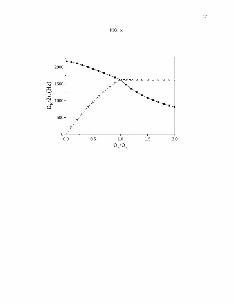
47

FIG. 5:

0.0 0.5 1.0 1.5 2.00

500

1000

1500

2000

ΩK/2

π (H

z)

Ωn/Ω

p

48

FIG. 6:

0 0.5 1 1.5 2Ω

n / Ω

p

0.9

1

1.1

1.2

1.3

ΩK

,A /

ΩK

σ = − 0.5

n

0 0.5 1 1.5 2Ω

n / Ω

p

σ = 0

p

p

n

ε = 0ε = 0.4ε = 0.7

0 0.5 1 1.5 2Ω

n / Ω

p

0.9

1

1.1

1.2

1.3

ΩK

,A /

ΩK

σ = 0.5

n

p

49

FIG. 7:

0 0.1 0.2 0.3 0.4 0.5ωM

-4

-2

0

log 10

|Ain

|

f s0

p1 s

1p

2s

2p

3s

3

50

FIG. 8:

0 0.1 0.20

0.2

0.4

0.6

0.8

ε

Re

ωM

a0.2a

0.1a

0

b0

b0.1

b0.2

51

FIG. 9:

0 0.2 0.4 0.6 0.8 1 0 0.2 0.4 0.6 0.8 1 0 0.2 0.4 0.6 0.8 1

0 0.2 0.4 0.6 0.8 1 0 0.2 0.4 0.6 0.8 1 0 0.2 0.4 0.6 0.8 1

a0 a

0.1 a0.2

b0.1b

0b

0.2

52

Tables

53

TABLE I:

model I model II model III

σn/mn 0.2 0.22 0.2

σp/mn 0.5 1.95 2

βn 2.5 2.01 2.3

βp 2.0 2.38 1.95

nc (fm−3) 1.3 1.21 0.93

pc (fm−3) 0.741 0.22 0.095

M/M⊙ 1.355 1.37 1.409

R (km) 7.92 10.19 10.076

Rc (km) — 8.90 —