RELATION BETWEEN THE FUTURES PRICE AND COST OF CARRY

By

Prof. B Ramesh Dean and Chairman BOS

Department of Commerce Goa University Goa – 403 205 Email: brames@rediffmail.com

Dr. Anilkumar Garag Director Belgaum Institute of Management Studies Belgaum – 591156 Email: anilgarag@airtelmail.in

INTRODUCTION - THE COST OF CARRY MODEL

The cost of carry model is a classical model which defines the relationship

between the spot price and the futures price. The cost of carry model assumes that

the price of a futures contract is nothing but the price of the underlying asset in

the spot market plus the cost of carrying the asset for the period of the futures

contract. The following paragraphs will explain, describe and derive the cost of

carry model.

A general principle that pervades the pricing of all financial assets is that of

arbitrage. The principle of arbitrage states that: any two assets having identical

characteristics trade at the same price. If this were not the case, selling the

higher priced asset and buying the lower priced asset can make a risk-free profit.

This is often referred to the law of one price.

The methods of pricing futures can be divided into two groups. The first method

relates to so-called carryable assets. These are assets that can be purchased in the

spot market at the same time as the futures contract is entered into and held

(carried) for the duration of the contract; examples include currencies, bonds,

equities, equity indices and commodities that have already been produced. The

second group of contracts relates to non-carryable asset; i.e., Assets that cannot

be carried, simply because they do not exist at the time the futures contract is

entered into. Indeed, some will only come into existence on the date that

coincides with the end of the futures contract’ life. An example is an interest rate

future where the underlying asset is the interest rate on a three-month deposit that

commences its life at the end of the future’s life. Some types of non-carryable

asset will come into existence at some time during the life of the future, but by

their very nature cannot be stored. Examples are insurance premium rates and

marine freight rates, both of which are the variable underlying some future

contracts.

The cash-and-carry arbitrage

When the underlying asset is a financial asset, it is reasonable to assume that

investors in the asset hold it only to make a financial gain in return for bearing the

associated risk. Thus, in such circumstances, the fair price of the future is that

price at which arbitrage between the underlying asset and the derivative just

breaks even, there is no profit and no loss. If the derivative is overvalued, the

arbitragers will sell it, buy the underlying asset with borrowed funds and deliver

the underlying asset into the derivatives contract. On the other hand, if the

derivative is cheap, the arbitragers will buy it and sell short the underlying asset

against it. The short sale will be satisfied when the arbitrager receives the

underlying asset under the derivatives contract and delivers it into the short sale.

Such arbitrage transactions are known as cash and carry arbitrage.

Futures contracts provide for delivery of the underlying asset at the future date

(T). Whether the arbitrager uses own funds or borrowed funds for acquiring the

asset on that date (t) both the strategies result in holding the underlying asset at

the future rate; thus, both must have the same price today otherwise arbitrage

profits would be possible. Assuming that the assets does not earn any income nor

incur storage costs and r is the appropriate rate of interest for the period T - t,

which represents the life of the futures contract, the arbitrage free futures price

will be

)()1( tT

Ttt rPF (1.1)

Where

Ft is the price of the Futures contract on date t

Pt is the price of the underlying asset on date t

r is the appropriate interest rate for the period (T – t)

The Above equation (1.1) assumes a compound interest charge. But in Stock

markets where the stock prices (prices of underlying assets) change every

moment, a continuous compounding method is more useful and apt to the

circumstances.

Therefore the equation for ascertaining the futures price becomes:

)( tTr

tt ePF (1.2)

Where

Ft is the price of the Futures contract on date t

Pt is the price of the underlying asset on date t

r is the appropriate interest rate per annum for the period (T – t)

This leads us to a new generalization that is: The price of the Futures contract is

equal to the present price of the underlying asset plus the cost of carrying the asset

for the period (T-t) this can be represented as:

Ft = Pt + C (1.3)

Where C is the net cost of carry. The net cost of carry will take into account not

only the cost of funds borrowed to purchase the asset, but also the storage costs

(i.e. custody charges) and any other income flowing from the asset during the life

of the future. If storage costs, borrowing costs and income accrue at the same

time, the whole net cost of carry can be treated as an annual rate and if continuous

compounding is assumed then the equation 3.3 would become

(1.4)

Where C= cost of carry is expressed as a rate and quoted in decimals.

F = Futures price of the contract

P = Spot price of the contract

e = 2.7181

T = Date of expiry of the contract

t = Date of the contract price

The above equation defines a straight forward relation between the cost of carry

and the futures price. we calculate the cost of carry for every day for every

contract.

After calculating the cost of carry, does this cost of carry have any significant

relation with the futures price of the contracts? If the cost of carry goes increases,

does the futures price also increase? Does the change in cost of carry bring about

a corresponding change in the futures price? These are the questions that are

attempted to be answered in the following paragraphs.

RESEARCH PROBLEM

“To find out the relationship between the change in cost of carry of the future

prices of stocks on the National Stock Exchange and the change in futures price”

OBJECTIVES

To understand the behaviour of the futures prices of single stock futures vis-à-vis the cost

of carry

To understand the behaviour of the futures prices of NIFTY futures vis-à-vis the cost of

carry.

HYPOTHESES

There is a strong and positive correlation between the change in futures price and the

change in cost of carry in single stock futures

There is a strong and positive correlation between the change in NIFTY futures and the

change in cost of carry in NIFTY futures.

METHOD OF STUDY

Data Collection:

Sixteen liquid stocks were selected on a random basis from the universe of the

S&P CNX NIFTY along with the NIFTY itself. The futures prices for the months

of the contract expiring in July 2002 to June 2006 were considered for computing

the cost of carry in the stock on a daily basis.

The data collected for the sixteen stocks and NIFTY consisted of 48 files each for

each stock. Each file contained the OPEN, HIGH, LOW, CLOSE, Last Traded

Price, Settlement Price, Number of Contracts Traded, open interest and Change in

Open Interest for the specified Contract. The data was available on an average for

about 90 days per contract, from the day of introduction of the contract to the

expiry of the contract. It was observed that these contracts were traded thinly until

they became near-month contracts. Therefore only the data pertaining to the near

month contracts was selected and a single data set of near month contract prices

was prepared for each of these stocks. The data for the day of expiry was omitted

and data for the next contract was included for the day of contract expiry as the

cost of carry is expected to be zero on the contract expiry date for a specific

contract.

The stocks selected were:

Table 1.1: List of the companies selected for analysis

Company Name Industry Symbol

Associated Cement Companies Ltd. Cement and cement

products

ACC

Bajaj Auto Ltd. Automobiles - 2 and 3

wheelers

BAJAJAUTO

Bharti Airtel Ltd. Telecommunication –

services

BHARTIAIRTEL

Bharat Heavy Electricals Ltd. Electrical equipment BHEL

Cipla Ltd. Pharmaceuticals CIPLA

GAIL (India) Ltd. Gas GAIL

Housing Development Finance

Corporation Ltd.

Finance – housing HDFC

Hero Honda Motors Ltd. Automobiles - 2 and 3

wheelers

HEROHONDA

Infosys Technologies Ltd. Computers – software INFOSYSTCH

I T C Ltd. Cigarettes ITC

National Aluminium Co. Ltd. Aluminium NATIONALUM

Reliance Industries Ltd. Refineries RELIANCE

State Bank of India Banks SBIN

Tata Motors Ltd. Automobiles - 4

wheelers

TATAMOTORS

Tata Steel Ltd. Steel and steel

products

TATASTEEL

Tata Tea Ltd. Tea and coffee TATATEA

NIFTY - NIFTY

The open interest was found to have been picked up whenever the contract

became a near month contract. Therefore only the near month contracts and their

open interest was considered for calculations

LIMITATIONS

The study is limited to the 17 futures contracts selected for a period of June 2002

June 2006. The underlying dynamics of the economy were changing fast and the

popularity of futures trading were just picking up in these years and therefore this

study would at best describe the phase of evolution of futures market in India.

The study aims to find out whether cost of carry and the change in change in cost

of carry in a stock futures contract and index contract have any effect on the

change in the prices of the contract. Since the cost of carry equation is a proven

theory and has been the cornerstone of all the research on futures contracts and

derivatives in general it is not an attempt to prove or disprove a theory. This is

attempt to find out how much truth is there in the market perception that futures

prices behave according to the behaviour of the cost of carry.

DATA COLLECTION AND CONSOLIDATION:

The futures Price data collected from the NSE website (www.nseindia.com) was

available in the form of contract wise price volume data for the specific contract.

The data for the above said stocks and the NIFTY was downloaded from the NSE

website. Data for each stock was contained in a contract-wise file making it up to

48 files per stock. These 48 files were further pruned to one month or near month

contract data and then merged into a single data set containing the one month or

near month contract price data for the period of 28 June 2002 to 29 June 2006.

The spot prices for all the stocks for the period from 28 June 2002 to 29 june 2006

were downloaded from the NSE website and placed alongside the futures data for

the purpose of consolidation.

Thus each data set had the following fields: SYMBOL, EXPIRY DATA, DATE

OF TRADE, DAYS TO EXPIRY, FUTURES CLOSE, SPOT CLOSE and OPEN

INTEREST.

DATA ANALYSIS

Correlation

In determining the correlation we use the measure of linear correlation. The

population parameter is denoted by the Greek letter rho and the sample statistic is

denoted by the roman letter r and is given by the equation 1.1. In our analysis

when x denotes change in COST OF CARRY, y denotes change in FUTURES

PRICE.

Determination of Change in FUTURES PRICE

The Change in futures price is found by using the following simple equation

1

1

t

tt

F

FFF (1.5)

Where

F is the change in futures price.

Ft is the closing futures price of the day.

Ft-1 is the closing futures price of the previous day.

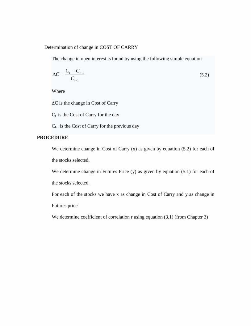
Determination of change in COST OF CARRY

The change in open interest is found by using the following simple equation

1

1

t

tt

C

CCC (5.2)

Where

C is the change in Cost of Carry

Ct is the Cost of Carry for the day

Ct-1 is the Cost of Carry for the previous day

PROCEDURE

We determine change in Cost of Carry (x) as given by equation (5.2) for each of

the stocks selected.

We determine change in Futures Price (y) as given by equation (5.1) for each of

the stocks selected.

For each of the stocks we have x as change in Cost of Carry and y as change in

Futures price

We determine coefficient of correlation r using equation (3.1) (from Chapter 3)

FINDINGS

Table 1.2: Table of correlation between Change in Futures Price and change in Cost of Carry

Name of Company Correlation Observations T

TINV

(99%) H0: p=0

ACC 0.03231 1006 1.02 2.81324 ACCEPT

Bajaj Auto -0.01891 1006 -0.60 2.81324 ACCEPT

Bharti Airtel -0.05683 283 -0.95 2.82921 ACCEPT

BHEL -0.07403 1006 -2.35 2.81324 ACCEPT

Cipla -0.00765 1006 -0.24 2.81324 ACCEPT

Gail -0.01169 652 -0.30 2.81662 ACCEPT

Hdfc 0.015114 951 0.47 2.81360 ACCEPT

Hero Honda -0.04797 812 -1.37 2.81473 ACCEPT

Infosys 0.044636 960 1.38 2.81354 ACCEPT

ITC -0.0259 998 -0.82 2.81329 ACCEPT

Nifty 0.031105 858 0.91 2.81431 ACCEPT

Nalco -0.107954 1006 -3.44 2.81324 REJECT

Reliance 0.027795 1006 0.88 2.81324 ACCEPT

SBI -0.065147 1006 -2.07 2.81324 ACCEPT

Tata Motors -0.030452 1006 -0.97 2.81324 ACCEPT

Tata Power 0.048062 1006 1.52 2.81324 ACCEPT

Tata Steel 0.030173 1006 0.96 2.81324 ACCEPT

Tata Tea 0.068696 1006 2.18 2.81324 ACCEPT

ACCEPT 17

REJECT 1

The Table 1.1 depicts the distribution of the correlation between the change in

cost of carry and the change in futures price and it can be observed from the table

that the correlation coefficient hovers around ZERO. A T-test to confirm our

observations also yields the same results that the correlation between eh change in

futures price and the change in cost of carry is near ZERO. This leads us to the

conclusion that the change in futures price cannot be explained by the change in

cost of carry at all. This also means that popular conception that futures prices

vary with the change in cost of carry is not true. The chart below describes the

distribution of correlation.

Chart 1.1 Correlation between the change in cost of carry and the change in

futures price.

CONCLUSION

It is clear from the chart 1.1 and the table 1.1 that the correlation between the

change in cost of carry and the change in futures price of the futures contracts

selected as sample from the universe of the NIFTY constituents has a range of -

0.1079 for NALCO and 0.0687 for Tata Tea futures. This leads us to conclude

that the variables are not related to each other and they are independent of each

other.

Hypothesis 1: There is a strong and positive correlation between the change in futures

price and the change in cost of carry in single stock futures. The hypothesis is rejected as

the correlation coefficient hovers around ZERO. The Null hypothesis that there is no

correlation between the change in cost of carry and change in futures price stands

accepted in 15 out of the 16 single stock futures contracts.

Hypothesis 2: There is a strong and positive correlation between the change in NIFTY

futures and the change in cost of carry in NIFTY futures. The hypothesis is rejected as the

correlation coefficient hovers around ZERO, as the Null hypothesis stands accepted in

case of Nifty futures contracts.

This relationship or the absence of it suggests that the change in cost of carry does

not dictate any change in the futures prices. This also means that the cost of carry

does not have any directional information. We can conclude from this analysis

that cost of carry changes as and when the cost of money increases or decreases in

the economy and it has no bearing over the direction of the market. Thus we can

also say that a change in cost of carry will not lead to a change in futures price in

any direction.

Bibliography:

Terry J. Watsham, (1998) Futures and Options in Risk Management, Thompson,.

John C. Hull, (2002), Options, Futures, & other Derivatives, Pearson Education Asia,.

Richard I. Levin & David S. Rubin, (1992) Statistics for Management, Prentice Hall,.

Sharon Jose (2005) Components of Cost of Carry for Index Futures, Treasury

Management 2 ;

Dr. L.C.Gupta, Derivatives in India: A Framework of Economic Purpose (Committee

Draft Report Part-I)

Richard Heaney, (1995), A Test of the Cost of Carry Relationship using 90-Day Bank

Accepted Bills and the All Ordinaries Share Price Index: Australian Journal of

Management, June; pp 75-104.

Don M Chance, Another look at the forward-futures price differential in LIBOR markets:

E. J. Ourso College of Business Administration, Louisiana State University,

http://nseindia.com/content/fo/fobhav_arch.htm

http://nseindia.com/marketinfo/eod_information/bidbor.jsp