arX

iv:c

ond-

mat

/001

2511

v4 [

cond

-mat

.sup

r-co

n] 6

Aug

200

1

Finite Temperature Time-Dependent Effective Theory for

the Phase Field in two-dimensional d-wave Neutral Superconductor

S.G. Sharapov∗ and H. Beck†

Institut de Physique, Universite de Neuchatel, 2000 Neuchatel, Switzerland

V.M. Loktev‡

Bogolyubov Institute for Theoretical Physics, Metrologicheskaya Str. 14-b, Kiev, 03143, Ukraine

(Dated: March 15, 2001)

We derive finite temperature time-dependent effective actions for the phase of the pairing field,which are appropriate for a 2D electron system with both non-retarded d- and s-wave attraction.As for s-wave pairing the d-wave effective action contains terms with Landau damping, but theirstructure appears to be different from the s-wave case due to the fact that the Landau damping isdetermined by the quasiparticle group velocity vg, which for d-wave pairing does not have the samedirection as the non-interacting Fermi velocity vF . We show that for d-wave pairing the Landauterm has a linear low temperature dependence and in contrast to the s-wave case are important forall finite temperatures. A possible experimental observation of the phase excitations is discussed.

PACS numbers: 74.20.Fg, 74.20.De, 74.72.-h, 11.10.Wx

I. INTRODUCTION

The microscopic derivation of the effective time-dependent Ginzburg-Landau (GL) theory continues to attractattention since an early paper by Abrahams and Tsuneto [1]. Whereas the static GL potential was derived [2] fromthe microscopic BCS theory soon after its introduction, the time-dependent GL theory is still a subject of interest (see[3, 4] for a review on the problem’s history). One of the reasons for this is the presence of Landau damping terms inthe effective action. For s-wave superconductivity these terms are singular at the origin of energy-momentum space,and consequently they cannot be expanded as a Taylor series about the origin. In other words, these terms do nothave a well-defined expansion in terms of space and time derivatives of the ordering field and therefore they cannotbe represented as a part of a local Lagrangian. We recall that at T = 0 and for the static (time-independent) casethe Landau damping vanishes, so that either at T = 0 one still has a local well-defined time-dependent GL theory orfor T 6= 0 the familiar static GL theory exists. It is known, however, that for s-wave superconductivity even thoughthe Landau terms do exist, they appear to be small compared to the main terms of the effective action in the largetemperature region 0 < T . 0.6Tc [4], where Tc is the superconducting transition temperature. This is evidentlyrelated to the fact that only thermally excited quasiparticles contribute to the Landau damping. The number of suchquasiparticles at low temperatures appears to be a small fraction of the total charge carriers number in the s-wavesuperconductor due to the nonzero superconducting gap ∆s which opens over all directions on the Fermi surface.

For a d-wave superconductor there are four Dirac points (nodes) where the superconducting gap ∆d(k) becomeszero on the Fermi surface. The presence of the nodes increases significantly the number of the thermally excitedquasiparticles at given temperature T comparing to the s-wave case. Therefore one can expect that the Landaudamping should be stronger for superconductors with a d-wave gap which is commonly accepted to be the case of high-temperature superconductors (HTSC) [5]. Moreover, it is believed that at temperatures T ≪ Tc,these quasiparticlesare reasonably well described by the Landau quasiparticles, even though such an approach fails in these materials athigher energies [6]. This is the reason why one can hope that a generalization of the BCS-like approach [4] for the2D d-wave superconductivity may be relevant to the description of the low-temperature time-dependent GL theoryin HTSC.

In this work we derive such a theory from a microscopical model with d-wave pairing extending the approach of [4]developed for s-wave superconductivity. As known from [1] the physical origin of the Landau damping is a scatteringof the thermally excited quasiparticles (“normal” fluid) with group velocity vg from the excitations of phase (or θ-)

quantums. Such conversion occurs only if the Cerenkov condition, Ω = vgK for the energy Ω and momentum K of

∗On leave of absence from Bogolyubov Institute for Theoretical Physics, Kiev, Ukraine; Electronic address: Sergei.Sharapov@unine.ch†Electronic address: Hans.Beck@unine.ch‡Electronic address: vloktev@bitp.kiev.ua

2

the θ-excitation is satisfied. This phenomenon in superconductivity is also called Landau damping since its equivalentin the plasma theory was originally obtained by Landau (see e.g. [7]).

To emphasize the difference between the Landau damping for s- and d-wave pairing, we also derive for the compar-ison the corresponding terms for a 2D s-wave superconductor. In addition we compare 2D expressions obtained herewith the 3D s-wave case studied in [4]. The collective phase oscillations in charged d-wave superconductor for cleanand dirty cases were recently studied in [8]. Due to the complexity of the corresponding equations they were solvednumerically, neglecting damping of the phase excitations. Thus our fully analytical treatment can be very useful forfurther studies of the phase excitations. We also mention a recent paper [9] where the effective action for the phasemode in the d-wave superconductor was obtained using the cumulant expansion. The Landau terms were neglectedin [9], but the effect of Coulomb interaction was taken into account.

Our main results can be summarized as follows.1. We find that the main physical difference between the s- and d-wave cases is related to the fact that for d-wave

superconductivity the direction of the quasiparticle group velocity vg(k) ≡ ∂E(k)/∂k (E(k) is the quasiparticledispersion law) does not coincide with the Fermi velocity vF [6, 10] and a gap velocity v∆ ≡ ∂∆d(k)/∂k also entersinto the Cerenkov condition along with vF .

2. We show that the intensity of the Landau damping has a linear temperature dependence at low T with acoefficient expressed in terms of the anisotropy αD ≡ vF /v∆ of the Dirac spectrum E(k) =

√

v2F k

21 + v2

∆k22 . Here

k1 (k2) are the projections of the quasiparticle momentum on the directions perpendicular (parallel) to the Fermisurface. The parameters vF , v∆ and αD proved to be very convenient both in the theory, for example, of the transportphenomena [6], ultrasonic attenuation [10] in d-wave superconductors and for the analysis of various experiments [11].

3. We find that the Landau damping is sensitive to the direction of the phason momentum. In particular, for agiven node the Landau damping is possible only if the components of the phason momentum K = (K1,K2) (which are

defined exactly as the components of the quasiparticle momentum above) satisfy the condition |Ω| <√

v2FK

21 + v2

∆K22 .

4. We derive a simple approximate representation for the Landau damping terms which can be useful for furtherstudies of the d-wave superconductors.

5. We derive an approximate expression for the propagator of the Bogolyubov-Anderson mode which includes theLandau damping.

6. Concerning the mathematical formalism used in the paper, we adapt the bilocal Hubbard-Stratonovich fieldmethod of [12] to the d-wave pairing. Additionally we adjust the technique of the derivative expansion for the “phaseonly” action (see [4] and Refs. therein) for the model with the tight-binding spectrum.

The paper is organized as follows: In Section II we present our model and write down the partition function usinga bilocal Hubbard-Stratonovich field. In Section III, we introduce the modulus-phase variables and represent theeffective “phase only” action as an infinite series. It appears that the low-energy phase dynamics is contained in thefirst two terms which are evaluated, respectively, in Sections IV and V with some details considered in Appendix A.The effective Lagrangians for the d- and s-wave cases without the Landau damping are discussed in Section VI. InSection VII we derive the damping terms and in detail compare d- and s-wave cases. The approximate forms of theeffective action and θ- propagator are considered in Section VIII. Section IX presents our conclusions and commentson a possible experimental observation of the phase excitations.

II. MODEL

Let us consider the following action

S = −∫ β

0

dτ

[

∑

σ

∫

d2rψ†σ(τ, r)∂τψσ(τ, r) +H(τ)

]

, r = (x, y) , β ≡ 1

T, (1)

where the Hamiltonian H(τ) is

H(τ) =∑

σ

∫

d2rψ†σ(τ, r)[ε(−i∇)− µ]ψσ(τ, r)

− 1

2

∑

σ

∫

d2r1

∫

d2r2ψ†σ(τ, r2)ψ

†σ(τ, r1)V (r1; r2)ψσ(τ, r1)ψσ(τ, r2) .

(2)

Here ψσ(τ, r) is a fermion field with the spin σ =↑, ↓, σ ≡ −σ, τ is the imaginary time and V (r1; r2) is an attractivepotential. For the sake of the simplicity we consider the dispersion law, ε(k) = −2t(cos kxa+ cos kya) for a model ona square lattice with the constant a including the nearest-neighbor hopping t only. This, however, is not an essential

3

restriction because the final results for the d-wave case will be formulated in terms of the non-interacting Fermivelocity vF ≡ ∂ε(k)/∂k|k=kF

and the gap velocity v∆ defined in the Introduction.The bilocal Hubbard-Stratonovich fields Φ(τ, r1; r2) and Φ†(τ, r1; r2) (see e.g. [12]) can be utilized to study the

model (1), (2)

exp

[

∫ β

0

dτ

∫

d2r1

∫

d2r2ψ†↑(τ, r2)ψ

†↓(τ, r1)V (r1; r2)ψ↓(τ, r1)ψ↑(τ, r2)

]

=

∫

DΦ†(τ, r1; r2)DΦ(τ, r1; r2) exp

[

−∫ β

0

dτ

∫

d2r1

∫

d2r21

V (r1; r2)|Φ(τ, r1; r2)|2

+

∫ β

0

dτ

∫

d2r1

∫

d2r2(Φ†(τ, r1; r2)ψ↓(τ, r1)ψ↑(τ, r2) + ψ†

↑(τ, r1)ψ†↓(τ, r2)Φ(τ, r1; r2))

]

.

(3)

On the right hand side, 1/V (r1; r2) is understood as numeric division, no matrix inversion being implied. Thehermitian conjugate of Φ(τ, r1; r2) includes the transpose in the functional sense, i.e. Φ†(τ, r1; r2) ≡ [Φ(τ, r2; r1)]

∗.Thus in the Nambu variables

Ψ(τ, r) =

(

ψ↑(τ, r)

ψ†↓(τ, r)

)

, Ψ†(τ, r) =(

ψ†↑(τ, r) ψ↓(τ, r)

)

(4)

the partition function can be written as

Z =

∫

DΨ†DΨDΦ†DΦ exp

∫ β

0

dτ

∫

d2r1

∫

d2r2

[

− 1

V (r1; r2)|Φ(τ, r1; r2)|2

+ Ψ†(τ, r1)(−∂τ − τ3ξ(−iτ3∇))Ψ(τ, r2)δ(r1 − r2)

+Φ†(τ, r1; r2)Ψ†(τ, r1)τ−Ψ(τ, r2) + Ψ†(τ, r1)τ+Ψ(τ, r2)Φ(τ, r1; r2)

]

(5)

where ξ(−iτ3∇) ≡ ε(−iτ3∇)− µ and τ3, τ± = (τ1 ± iτ2)/2 are Pauli matrices.In general an electron-electron attraction on the nearest-neighbor lattice sites can be considered (see, for example,

[13, 14]). The momentum representation for this interaction contain in the pairing channel extended s-, d- and evenp-wave pairing terms:

V (k− k′) = V [cos(kx − k′x)a+ cos(ky − k′y)a]

=V

2(cos kxa+ cos kya)(cos k′xa+ cos k′ya) +

V

2(cos kxa− cos kya)(cos k′xa− cos k′ya)

+ V (sin kx sink′x + sin ky sink′y).

(6)

Motivating by HTSC we consider here d-wave pairing only, so that for the Fourier transform of the pairing potentialV (r1 − r2) we use

V (k− k′) = Vd(cos kxa− cos kya)(cos k′xa− cos k′ya) . (7)

As was mentioned in Introduction, we will compare the main results for the d-wave case with the simplest 2Dcontinuum s-wave pairing model (see e.g. [15] and the review [16]) which has a quadratic dispersion law ε(k) = k2/2mand a local attraction V (r1 − r2) = V δ(r1 − r2).

III. THE EFFECTIVE ACTION

While for the model with the local four-fermion attraction [4, 15] the modulus-phase variables could be introducedexactly, one should apply an additional approximation for treating the present model.

Let us split the charged fermi-fields ψ(τ, r) and ψ†(τ, r) in (5) into the neutral fermi-field χ(τ, r) [17] and chargedBose-field exp[iθ(τ, r)/2]

ψσ(τ, r) = χσ(τ, r) exp[iθ(τ, r)/2] , ψ†σ(τ, r) = χ†

σ(τ, r) exp[−iθ(τ, r)/2] . (8)

It is clear that the terms containing δ(r1− r2) in (5) can be treated similarly to the old model and the problem ariseswhen one deals with the Hubbard-Stratonovich field. To consider this field we introduce the relative r = r1 − r2

4

and center of mass coordinates R = (r1 + r2)/2. Now we can introduce the modulus-phase representation for theHubbard-Stratonovich field

Φ(τ, r1, r2) ≡ Φ(τ,R, r) = ∆(τ,R, r) exp[iθ(τ,R, r)] , (9)

where ∆(R, r) is the modulus of the Hubbard-Stratonovich field and θ(R, r) is its phase.Assuming that the global phase θ(R, r) varies slowly over distances on the order of a Cooper pair size and thus is

not sensitive to the inner pair structure described by the relative variable r, we can rewrite (9) as

Φ(τ,R, r) ≈ ∆(τ,R, r) exp[iθ(τ,R)] . (10)

The approximation we made writing Eq. (10) is in fact equivalent to the Born-Oppenheimer approximation [18]which allows one to separate the dynamics of the Cooper pair formation described by the relative coordinate r in∆(τ,R, r) from the motion of the superconducting condensate described by the center mass coordinate R in θ(τ,R).If the condensate motion is slow enough this separation becomes possible because the dynamics of the Cooper pairformation can always follow the motion of the condensate. Using the lattice language one can also say about (10)that the bond phase is replaced by the site phase [19].

Applying the transformations (10) and (8) to the terms with the Hubbard-Stratonovich field in (3) we obtain (theimaginary time τ is omitted)

Φ†(R; r)ψ↓(r1)ψ↑(r2) = Φ†(R; r)χ↓(r1) exp

[

iθ(R + r/2)

2

]

χ↑(r2) exp

[

iθ(R− r/2)

2

]

≈ ∆(R; r) exp[−iθ(R)]χ↓(r1)χ↑(r2) exp[

iθ(R) +rα2

rβ2∇α∇βθ(R)

]

≈ ∆(R; r)χ↓(r1)χ↑(r2) ,

(11)

where we used the assumption (or hydrodynamical, long wavelength approximation, see [20]) that θ(R) varies slowly,θ(R)≫ ξ20(∇θ(R))2. Here ξ0 is the coherence length which for the BCS theory coincides with an average pair size.

Then the partition function in the modulus-phase variables is

Z =

∫

∆D∆Dθ exp[−βΩ(∆, ∂θ)] , (12)

where the effective potential

βΩ(∆, ∂θ) =

∫ β

0

dτ

∫

d2r1

∫

d2r2∆2(τ,R, r)

V (r1 − r2)− TrLnG−1 (13)

with

G−1 = G−1 − Σ , (14)

G−1(τ1, τ2; r1, r2) ≡ 〈τ1, r1|G−1|τ2, r2〉

=[

−I∂τ1− τ3ξ(−iτ3∇1)

]

δ(τ1 − τ2)δ(r1 − r2) + τ1∆(τ1 − τ2,R, r) ;(15)

〈τ1, r1|Σ|τ2, r2〉 =

[

τ3

(

i∂τ1

θ

2+ ta2 (∇x1

θ)2

4cos(−ia∇x1

) + (x→ y)

)

+I

(

− ita2∇2

x1θ

2cos(−ia∇x1

) + ta∇x1θ sin(−ia∇x1

) + (x→ y)

)]

δ(τ1 − τ2)δ(r1 − r2) .

(16)

Thus the gauge transformation (8) resulted in the separation of the dependences on ∆ and θ, viz. θ is present onlyin Σ. The similar method of the derivative expansion was used before in [4, 21]. As pointed out in [4] the methodallows to maintain explicitly the Galilean invariance (the Landau terms break it) and the continuity equation, whilethe expansion Φ(x) = ∆+Φ1(x)+ iΦ2(x) used recently in [8] demands the additional enforcement of the conservationlaws [22].

Since the low-energy dynamics in the phase in which ∆ 6= 0 is determined by the long-wavelength fluctuationsof θ(x), only the lowest order derivatives of the phase such as ∇θ, ∂τθ and ∇2θ need be retained in what follows.However, to take into account the tight-binding electron spectrum the operators sin(−ia∇) and cos(−ia∇) must be

5

kept. Thus in Σ we have omitted higher order terms in ∇θ, but in order to keep all relevant terms in the expansionof sin(−ia∇) the necessary resummation was done [23]. One can easily see that for the quadratic dispersion law2t → 1/(ma2), cos(−ia∇) → 1 and sin(−ia∇) → −ia∇, so that Eq. (16) reduces to the known expression from[4, 21]. Thus we arrive at the one-loop effective action

Ω ≃ Ωkin(v, µ, T,∆, ∂θ) + ΩMF

pot(v, µ, T,∆) (17)

where

Ωkin(µ, T,∆, ∂θ) = TTr

∞∑

n=1

1

n(GΣ)n

∣

∣

∣

∣

∂∆/∂R=0

(18)

and

ΩMF

pot(µ, T,∆) =

(∫

d2R

∫

d2r∆2(r)

V (r)− TTr LnG−1

)∣

∣

∣

∣

∂∆/∂R=0

. (19)

Deriving the “phase only” action for the s-wave model it was possible to use ∆(R, r) = const [16]. The d-wave caseis more complicated because one should keep the dependence on the relative coordinate, ∆(R, r) ≈ ∆(r) which isrelated to the nontrivial pairing. The dependences of the gap ∆ on T , µ and Vd follow from the extremum conditionfor the mean-field (∂∆/∂R = 0) potential ∂ΩMF

pot/∂∆ = 0 which results in the usual BCS gap equation. For the d-wavepairing potential (7) one obtains

∆d(k) =∆d

2(cos kxa− cos kya) , (20)

where ∆d is the gap amplitude. In our case there is no need to solve the gap equation and express ∆d in terms of T ,µ and Vd since in what follows we will use ∆d, or more precisely the velocity v∆, as the input parameters and will beinterested in the low temperature (T ≪ ∆d) regime.

Thus assuming that ∆(R, r) does not depend on R one obtains for the frequency-momentum representation of (15)

G(iωn,k) = − iωnI + τ3ξ(k)− τ1∆(k)

ω2n + ξ2(k) + ∆2(k)

, (21)

where ∆(k) is given by (20) and ωn = π(2n+ 1)T is fermionic (odd) Matsubara frequency.The phase dynamics is contained in the kinetic part Ωkin of the effective action which only involves the single

degree of freedom θ. As discussed in [4], it is enough to restrict ourselves to terms with n = 1, 2 in the infinite seriesin (18) since at T = 0 this would give the right answer for a local time-dependent GL functional which involves thederivatives not higher than (∇θ)4 and (∂tθ)

2.

IV. THE FIRST ORDER TERM OF THE EFFECTIVE ACTION AND THE NODAL APPROXIMATION

In this section we calculate the first (n = 1) term of the sum appearing in (18):

Ω(1)kin = TTr[GΣ]

= T

∫ β

0

dτ

∫

d2r

T

∞∑

n=−∞

∫

d2k

(2π)2tr[G(iωn,k)τ3]

(

i∂τθ

2+ta2

4(∇xθ)

2 cos kxa+ta2

4(∇yθ)

2 cos kya

)

.(22)

Summing over Matsubara frequencies, one obtains

Ω(1)kin = T

∫ β

0

dτ

∫

d2r

[∫

d2k

(2π)2n(k)

(

i∂τθ

2+m−1

xx (k)(∇xθ)

2

8+m−1

yy (k)(∇yθ)

2

8

)]

(23)

with m−1xx (k) ≡ ∂2ξ(k)/∂k2

x, m−1yy (k) ≡ ∂2ξ(k)/∂k2

y and

n(k) = 1− ξ(k)

E(k)tanh

E(k)

2T, E(k) =

√

ξ2(k) + ∆2(k) . (24)

6

For T ≪ ∆d linearizing the quasiparticle spectrum about the nodes and defining a coordinate system (k1, k2) at

each node with k1 (k2) perpendicular (parallel) to the Fermi surface, we can replace the momentum integrationin (23) by an integral over the k-space area surrounding each node [6]. If we further define a scaled momentump = (p1, p2) = (p, ϕ) we can let

∫

d2k

(2π)2→

4∑

j=1

∫

dk1dk2

(2π)2→

4∑

j=1

∫

d2p

(2π)2vF v∆=

4∑

j=1

∫ pmax

0

pdp

2πvF v∆

∫ 2π

0

dϕ

2π, pmax =

√πvF v∆ , (25)

where p1 ≡ vF k1 = ε(k) = p cosϕ, p2 ≡ v∆k2 = ∆d(k) = p sinϕ and p =√

p21 + p2

2 =√

v2Fk

21 + v2

∆k22 = E(k).

Note that for the particular square lattice model used above those velocities are vF = 2√

2ta and v∆ = ∆da/√

2respectively.

Using (25) one can express Eq. (23) in terms of vF and v∆

Ω(1)kin = T

∫ β

0

dτ

∫

d2r

[

inf∂τθ

2+

∫ pmax

0

pdp

2πvF v∆

∫ 2π

0

dϕ

2πtanh

p

2T

a2p cos2 ϕ

4(∇θ)2

]

≈ T∫ β

0

dτ

∫

d2r

[

inf∂τθ

2+

√πvF v∆

48a(∇θ)2

]

,

(26)

where

nf =

∫

d2k

(2π)2n(k) (27)

is the density of carriers. We note that due to the slow convergence of the integrand in (26) the final expressiondepends explicitly on the value of the momentum cutoff pmax which was defined in [6] in such a way that the areaof the new integration region over 4 Brillouin sub-zones (see Fig. 1) is the same as that of the original Brillouinzone. Going from Eq. (23) to (26) we essentially replace the averaging over the true Fermi surface of the system bythe averaging over 4 nodal sub-zones. The validity of this approximation can only be justified if the correspondingintegrals contain the derivative of the Fermi distribution nF (k) which is highly peaked in the vicinity of the nodes.This appears to be the case of the temperature dependent parts of the phase stiffness J(T ), compressibility K(T )and the Landau damping terms. For the zero temperature values J(T = 0) and K(T = 0) the nodal approximationis not well justified. However, as we show in Sec. VI, this approximation can be justified a forteriory for their ratio(see Fig. 2) which determines the velocity of the Bogolyubov-Anderson-Goldstone mode. Finally, we stress that afterapproximation is used, it is impossible to recover the s-wave limit by putting v∆ → 0.

V. THE SECOND ORDER TERM OF THE EFFECTIVE ACTION

Let us evaluate the trace of the second term in expansion (18):

Ω(2)kin =

T

2Tr[GΣGΣ] . (28)

Substituting (16) into (28) we obtain that

Ω(2)kin = Ω

(2)kinθΩ2

nθ+ Ω(2)kinθK2θ+ Ω

(2)kinθKΩnθ , (29)

where using θ · · · θ we denoted symbolically that the corresponding term of (28) is either diagonal (i.e. its frequency-momentum representation contains θ(iΩn,K)Ω2

nθ(−iΩn,−K) or θ(iΩn,K)K2θ(−iΩn,−K)) as

βΩ(2)kinθΩ2

nθ =T

2

∞∑

n=−∞

∫

d2K

(2π)2θ(iΩn,K)

(

−Ω2n

4

)

θ(−iΩn,−K)T

∞∑

l=−∞

∫

d2k

(2π)2π33(iΩn,K; iωl,k) ; (30)

βΩ(2)kinθK2θ =

T

2

∞∑

n=−∞

∫

d2K

(2π)2θ(iΩn,K)K2

xθ(−iΩn,−K)×

T

∞∑

l=−∞

∫

d2k

(2π)2π00(iΩn,K; iωl,k)(ta)2 sin(kx −Kx/2)a sin(kx +Kx/2)a+ (x→ y)

(31)

7

or mixed

βΩ(2)kinθKΩnθ = −T

∞∑

n=−∞

∫

d2K

(2π)2θ(iΩn,K)

KxΩn

2θ(−iΩn,−K)

× T∞∑

l=−∞

∫

d2k

(2π)2

[

π03(iΩn,K; iωl,k)ita

2sin(kx +Kx/2)a+ π30(iΩn,K; iωl,k)

ita

2sin(kx −Kx/2)a

]

+ (x→ y) .

(32)

In (30) - (32) we introduced the following short-hand notations

πij(iΩn,K; iωl,k) ≡ tr[G(iωl + iΩn,k + K/2)τiG(iωl,k−K/2)τj ] , τi = (τ0 ≡ I , τ3) . (33)

More generally, we can rewrite Eqs. (31) and (32) as follows

βΩ(2)kinθK2θ ≃ T

2

∞∑

n=−∞

∫

d2K

(2π)2θ(iΩn,K)

KαKβ

4θ(−iΩn,−K)Παβ

00 (iΩn,K) ; (34)

βΩ(2)kinθKΩnθ = −T

2

∞∑

n=−∞

∫

d2K

(2π)2θ(iΩn,K)

iΩnKα

4θ(−iΩn,−K) [Πα

03(iΩn,K) + Πα30(iΩn,K)] , (35)

where

Παβ00 (iΩn,K) ≡

∞∑

l=−∞

∫

d2k

(2π)2π00(iΩn,K; iωl,k)vFα(k)vFβ(k) ,

Πα03(iΩn,K) ≡

∞∑

l=−∞

∫

d2k

(2π)2π03(iΩn,K; iωl,k)vFα(k) ,

(36)

vFα(k) = ∂ξ(k)/∂kα, we used the approximation vFα(k) ≃ vFα(k ± K/2) and took into account that(1/2π)

∫

d2kvαvβ =∫

kdkv2δαβ/2. It is convenient to introduce here

Π33(iΩn,K) ≡∞∑

l=−∞

∫

d2k

(2π)2π33(iΩn,K; iωl,k) (37)

which would allow to rewrite (30) in the same fashion as (34).As one could notice the product of the Fermi velocities enters Eq. (34) via (36). There is nothing surprising in this

fact since this piece of the effective action is related to the paramagnetic current correlator 〈jαjβ〉 [9] and in its turnthe current operator, j contains the Fermi velocity vF (k). We will return to this point considering the Landau termwhich originates from (34), so that here we note only that the current correlator term along with the diamagneticterm ∼ (∇θ)2 in Eq. (22) form together the mean-field phase stiffness.

The matrix traces πij and the corresponding expressions for Πij are calculated in Appendix A. Although theexpressions for them are rather lengthy they have a clear physical interpretation which is also discussed in theAppendix.

VI. THE EFFECTIVE LAGRANGIAN AT T 6= 0 WITHOUT THE LANDAU TERMS

The contribution of the first order term to the effective action is given in (26). Concerning the second order term,we note that when the Landau terms are neglected it is enough to set Ωn = 0 inside Π in (30), (34) and (35). Tobe more precise, the Landau terms arise from the second line of Eqs. (A2) and (A3) which contains “dangerous”denominators 1/(E+ −E− ± iΩn). One can however notice that the second line of Eq. (A2) leads also to the regularterms which are proportional to the derivative dnF (E)/dE. These lead to the second term in the square brackets in(38) and the whole expression (39) shown below. For the s-wave superconductivity [4, 15] in the temperature region0 < T . 0.6Tc these terms are very small compared to the main terms. Although the contribution from these termsis still local, their presence breaks the Galilean invariance [4]. This is the reason why it was more natural for [4] to

8

treat them along with “true” Landau terms since they also originate from the same denominators of the second line of(A2) as was mentioned above. For the d-wave superconductivity this splitting, however, appears to be rather artificialsince these terms are not small even for low temperatures due to the presence of the nodal quasiparticles, so here wewill consider all regular terms.

For the regular terms from the second order term we obtain a local effective action, involving time and spacederivatives of θ(t, r):

βΩ(2)kin(∂tθ)

2 =i

2

∫

dΩ

2π

∫

d2K

(2π)2θ(Ω,K)

Ω2

4θ(−Ω,−K)Π33(0,K→ 0)

= iT

2

∫

dt

∫

d2r(∂tθ(t, r))

2

4

∫

d2k

(2π)2

[

−∆2(k)

E3(k)tanh

E(k)

2T− 1

2T

ξ2(k)

E2(k)cosh−2 E(k)

2T

]

,

(38)

βΩ(2)kin(∇θ)2 =

i

2

∫

dΩ

2π

∫

d2K

(2π)2θ(Ω,K)

KαKβ

4θ(−Ω,−K)Παβ

00 (0,K→ 0)

= iT

2

∫

dt

∫

d2r∇αθ(t, r)∇βθ(t, r)

4

∫

d2k

(2π)2

[

− 1

2Tcosh−2 E(k)

2T

]

vFα(k)vFβ(k)

(39)

and the mixed term (35) does not contribute to the regular part within the used approximation, since Πα30(0,K →

0) = 0. Evaluating (38) and (39) we performed the analytical continuation iΩn → Ω + i0 back to the real continuousfrequencies, so that t is the real time.

Using the nodal expansion (25) to calculate (38), (39) and adding (26) we finally obtain the regular effectiveLagrangian, LR such that βΩkin = −i

∫

dt∫

d2rLR(t, r) for T ≪ ∆d and ignoring the Landau terms:

LR = −nf

2∂tθ(t, r) +

K

2(∂tθ(t, r))

2 − J

2(∇θ(t, r))2 , (40)

where the phase stiffness J ≡ Jd,s and compressibility K ≡ Kd,s are

Jd =

√πvF v∆24a

− ln 2

2π

vF

v∆T , Kd =

1

4a√πvF v∆

. (41)

The linear time derivative term in (40) is important for the description of vortex dynamics (see [9] and Refs. therein),but we omit it in what follows. We stress that the second, temperature dependent term in Jd follows from Eq. (39)which contains the derivative of the Fermi distribution, dnF (E)/dE. Its presence, as we mentioned in Sec. IV, makesthe nodal approximation valid [6]. Since we consider only the low temperature T ≪ ∆d region, we restrict ourselvesby the values ∆d and v∆ at T = 0, so that all temperature dependences appear to be linear. For higher temperaturesit is necessary to take into account that ∆d(T ) and v∆(T ) are in fact decreasing functions of T .

It is useful to compare the stiffness and compressibility from (41) with those parameters derived in [15] for thecontinuum 2D model with s-wave pairing:

Js =nf

4m

1−∫ ∞

0

dx1

cosh2

√

x2 +∆2

s

4T 2

, Ks =m

4π. (42)

First of all one can see that for low temperatures the superfluid stiffness in (42) does not contain any term whichgoes to zero more slowly than exp(−∆s/T ), while (41) has a term proportional to T . The origin of this difference iswell-known and related to the presence of the nodal quasiparticles. Secondly, we can compare the values of the zerotemperature superfluid stiffness which for the continuum translationally invariant system has to be equal to nf/4m,so that all carriers participate in the superfluid ground state [25]. Since the presence of a lattice evidently breaksthe continuum translational invariance the superfluid density at T = 0 in the case of (41) is less than nf/4m, as canbe readily seen from (23). Finally, since we consider here a neutral system it has the Berezinskii-Kosterlitz-Thouless

(BKT) collective mode [26], Ω2 = v2K2 with v =√

J/K. One can see that for the continuum s-wave case v = vF /√

2and

v =

√

πvF v∆6

− 2 ln 2avF√π

√

vF

v∆T (43)

9

for the d-wave model on lattice at T ∼ 0. Eq. (43) gives rather simple approximate expression for the BKT modevelocity for the lattice model of d-wave superconductor. Comparing in Fig. 2 the results obtained for v(T = 0) usingEq. (43) with the numerical computation without the nodal approximation, we can see that that even being verysimple Eq. (43) predicts the correct behavior of v(T = 0).

Following [9] we estimate the upper values for the frequency Ω in (38) and the momentum K in (39). The“phase-only” effective action is appropriate for phase distortions whose energy is smaller than the condensationenergy, Econd ≃ N(0)∆2/2, where N(0) is the density of states. For the s-wave case (42) this leads to the following

restrictions: Ω < ∆s, vFK < ∆s and for the d-wave case (41): Ω < ∆d4

√

1/αD, vFK < ∆d4√αD, where αD is the

anisotropy of the Dirac spectrum defined in Introduction.

VII. THE IMAGINARY PART OF THE LANDAU TERMS FOR 2D d-WAVE AND s-WAVE CASES

The key values which are necessary for evaluation of the Landau terms are the differences E+ −E− and nF (E+)−nF (E−). Expanding in K,

E(k + K/2)− E(k−K/2) = vg(k)K , (44)

where the group velocity is given by

vg(k) = ∇kE(k) =1

E(k)[ξ(k)vF + ∆(k)v∆] . (45)

It is obvious that due to the gap k-dependence Eq. (44) differs from the s-wave case [4], where the difference is simply

E(k + K/2)− E(k−K/2) =ξ(k)

E(k)vF K (∆(k) = ∆s) . (46)

It is convenient to rewrite (44) and (45) in terms of the nodal approximation described after Eq. (25). In the vicinityof one of the nodes we have

vgK = vFK1 cosϕ+ v∆K2 sinϕ ≡ P cos(ϕ− ψ) , E(k±K/2)≪ ∆d , (47)

where the momentum K = (K1,K2) of θ-particle was also expressed in the nodal coordinate system k1, k2, so that

P 1 ≡ vFK1 = P cosψ, P 2 ≡ v∆K2 = P sinψ and P =√

(P 1)2 + (P 2)2 =√

v2FK

21 + v2

∆K22 . (We denoted the

components of P as P 1, P 2 to make them different from the node label Pj used in what follows.)The corresponding substitution in the integrals over K reads similarly to Eq. (25)

∫

d2K

(2π)2→

4∑

j=1

∫ Pmax

0

PjdPj

2πvF v∆

∫ 2π

0

dψj

2π, (48)

where Pmax is evidently related to the maximal value ofK discussed at the end of Sec. VI. Finally, we can approximatethe difference nF (E+)− nF (E−) as

nF (E+)− nF (E−) ≈ dnF (E)

dEvgK =

dnF (E)

dEP cos(ϕ− ψ) (49)

Having the differences (47) and (49) we can now derive the imaginary part for the Landau terms. In the subsequentsubsections we consider all three terms of Eq. (29) for d-wave pairing and compare them with their s-wave counterparts.We would like to note that the Landau terms have also the real part which for the 3D s-wave case was consider indetail in [4]. This real part consists of regular and irregular terms. The regular term was already taken into accountin Sec. VI and the irregular term is not considered in this paper.

10

A. Ω(2)kinθΩ2θ term

Let us consider firstly the contribution from Ω(2)kinθΩ2

nθ (see Eqs. (30) and (A2) for A−), which after the analyticalcontinuation iΩn → Ω + i0 takes the form

Im[iβΩ(2)kinθΩ2θ] ≈ −1

2

∫

dΩd2K

(2π)3θ(Ω,K)

Ω2

4θ(−Ω,−K)

×∫

d2k

(2π)21

2

(

1 +ξ2 −∆2

E2

)

Im2

vgK + Ω + i0

dnF (E)

dEvgK

≈4∑

j=1

∫

dΩ

2π

∫ Pmax

0

PjdPj

2πvF v∆

∫ 2π

0

dψj

2πθ(Ω,K)

Ω2

8θ(−Ω,−K)

×∫ pmax

0

pdp

2πvF v∆

∫ 2π

0

dϕ cos2 ϕδ(Pj cos(ϕ− ψj) + Ω)dnF (E)

dEPj cos(ϕ− ψj)

=

4∑

j=1

∫

dΩ

2π

∫ Pmax

0

PjdPj

2πvF v∆

∫ 2π

0

dψj

2πθ(Ω,K)

Ω2

8θ(−Ω,−K)

ln 2

π

T

vF v∆

× 1√

1− Ω2

P 2j

Ω

Pj

[

Ω2

P 2j

cos2 ψj +

(

1− Ω2

P 2j

)

sin2 ψj

]

Θ

(

1− |Ω|Pj

)

.

(50)

Here Θ(x) is the step function and we used the integral∫ ∞

0

pdp

2πvF v∆

1

2T

1

cosh2 p

2T

=ln 2

π

1

vF v∆T . (51)

Integrating over ϕ we had to take into account that there are two points where δ-function contributes into the integral:

cosϕ = −Ω/Pj, sinϕ =√

1− Ω2/P 2j and cosϕ = −Ω/Pj, sinϕ = −

√

1− Ω2/P 2j .

As we can see from the first equality in (50) the imaginary part develops when Ω = E+ − E− ≈ vgK. This

condition was interpreted in [1] as the “Cerenkov” irradiation (absorption) condition for the process: “thermallyexcited θ-fluctuation quantum (phason) + quasiparticle ←→ phason + quasiparticle” (or phason being absorbedand scattering thermally excited quasiparticles). As was discussed in [6], since definite energy is carried by thequasiparticles, this process is defined by their group velocity vg = ∂E(k)/∂k [1] as well as thermal and spin currents.

It is in fact a coincidence that for the s-wave superconductor the directions of vg and vF are the same, so that forthe 2D s-wave superconductor using (46) instead of (44) and (45) one can obtain

Im[iβΩ(2)kinθΩ2θ] = −1

2

∫

dΩd2K

(2π)3θ(Ω,K)

Ω2

4θ(−Ω,−K)

∫

d2k

(2π)22ξ2

E2Im

1

ξ

EvF K + Ω + i0

dn(E)

dE

ξ

EvF K

= −1

2

∫

dΩd2K

(2π)3θ(Ω,K)

Ω2

4θ(−Ω,−K)

∆smc

2π

∫ ∞

−∞

dy√

1− c2 1 + y2

y2

dn

dE

2|y|√

1 + y2Θ

(

|y|√

1 + y2− |c|

)

,(52)

where following [4] we used the notations y = ξ/∆s and c = Ω/vFK. Comparing (52) with the 3D case [4] (in the

notations of [4] the term we consider is related to the sum BL+CL) one can notice that the only difference between thecorresponding expressions is in the square root in the denominator of (52). It obviously originates from the differentmeasures for the angular integration in 2D and 3D where the extra sinϕ is present. Comparing also (50) and (52) onecan see that their main analytical structure appears to be the same, viz. ∼ Ω3/Pj for the d-wave case and ∼ Ω3/vFKfor the s-wave case, so that the momentum variables Pj and vFK do not appear in the numerator.

We note that the calculation of the ultrasonic attenuation αsound(T,K) in d-wave superconductors results in theexpression

αsound(T,K) ∼ Ω

2T

∫

d2k

(2π)2ξ2(k)

E2(k)

1

cosh2 E(k)

2T

δ(vgK) , (53)

11

which has the same structure as (50). This can be easily seen if one takes into account that for ultrasound frequencyrange Ω≪ vFK,∆d, so that the corresponding terms from Eq. (50) can be simplified as follows

δ(E+ − E− + Ω)[nF (E−)− nF (E+)] = δ(E+ − E− + Ω)[nF (Ω + E+)− nF (E+)] ≃ Ωδ(E+ − E−)nF (E)

dE(54)

leading to Eq. (53). This the reason why in the limit Ω/vFK → 0 the angular dependence of the Landau damping (50)which we consider in Sec. VIII would appear to be the same as the angular dependence of the ultrasonic attenuation[10].

B. Ω(2)kinθK2θ term

The contribution from Ω(2)kinθK2θ (see Eqs. (34) and (A2) for A−) can be treated in the same manner

Im[iβΩ(2)kinθK2θ] ≈ −1

2

∫

dΩd2K

(2π)3θ(Ω,K)

KαKβ

4θ(−Ω,−K)

×∫

d2k

(2π)21

2

(

1 +ξ2 + ∆2

E2

)

Im2

vgK + Ω + i0vFα(k)vFβ(k)

dnF (E)

dEvgK

≈4∑

j=1

∫

dΩ

2π

∫ Pmax

0

PjdPj

2πvF v∆

∫ 2π

0

dψj

2πθ(Ω,K)

P 2j cos2 ψj

8θ(−Ω,−K)

×∫ pmax

0

pdp

2πvF v∆

∫ 2π

0

dϕδ(Pj cos(ϕ− ψj) + Ω)dnF (E)

dEPj cos(ϕ− ψj)

=

4∑

j=1

∫

dΩ

2π

∫ Pmax

0

PjdPj

2πvF v∆

∫ 2π

0

dψj

2πθ(Ω,K)

P 2j cos2 ψj

8θ(−Ω,−K)

ln 2

π

T

vF v∆

× 1√

1− Ω2

P 2j

Ω

PjΘ

(

1− |Ω|Pj

)

(55)

and for the s-wave case

Im[iβΩ(2)kinθK2θ] = −1

2

∫

dΩd2K

(2π)3θ(Ω,K)

KαKβ

4θ(−Ω,−K)

∫

d2k

(2π)2Im

2

ξ

EvF K + Ω + i0

vFαvFβdn(E)

dE

ξ

EvF K

= −1

2

∫

dΩd2K

(2π)3θ(Ω,K)

Ω2

4θ(−Ω,−K)

∆smc

2π

∫ ∞

−∞

dy√

1− c2 1 + y2

y2

dn

dE

2(1 + y2)3/2

y2|y| Θ

(

|y|√

1 + y2− |c|

)

.

(56)

Let us now compare the expressions (55) and (56). Evidently their analytical structure is different since for the s-wavecase we have again that it is proportional to Ω3/vFK, while for d-wave pairing Pj enters the numerator, so that themain structure (excluding the measure of integration over Pj and the square root in the denominator) is ∼ ΩPj . Thisdifference originates from the angular integration in (55) and (56) which is performed using the δ-function. Since thearguments of the δ-function for the d- and s-wave cases are different we have obtained two different answers. Indeed,

for the s-wave case the argument is proportional to vF K that coincides with the product (vF K)2dnF (E)

dEvF K outside

the δ-function. (see Sec. V after Eq. (34), where the origin of the term ∼ (vF K)2 is discussed), so that the angularintegration removes K from the numerator. The d-wave case appears to be different since we have vgK inside the

δ-function and (vF K)2dnF (E)

dEvgK outside, so that the angular integration leaves Pj in the numerator. Despite the

fact that ΩPj looks substantially less singular than Ω/Pj, the first expression still remains nonanalytical near Pj ≈ 0

because it is expressed in terms of√

K2 the coordinate representation of which is the non-local operator√−∇2.

Thus physically the difference between the analytical form of the Landau damping in d- and s-wave superconductorsoriginates from the k-dependence of the gap ∆d(k) which in its turn makes the direction of the quasiparticle group

12

velocity vg different from the Fermi velocity vF . The last velocity, however, still enters the numerator of (55)since, as was already mentioned in Sec. V, it originates from the current-current correlator. The electrical current isproportional to vF , not vg because quasiparticles carry definite energy and spin, but do not carry definite charge.Therefore, the specific form of the Landau damping terms in a d-wave superconductor has the same physical origin asthe source of the extra terms in the thermal and spin conductivities [6] which are related to the presence in vg bothvF and v∆ components.

The s-wave Landau damping (56) itself can be again related to the 3D case [4], where it is expressed via the

difference BL − CL.

C. Ω(2)kinθKΩθ term

Finally we consider the contribution from Ω(2)kinθKΩθ (see Eqs. (35) and (A3)):

Im[iβΩ(2)kinθKΩθ] ≈ −1

2

∫

dΩd2K

(2π)3θ(Ω,K)ΩKαθ(−Ω,−K)

×∫

d2k

(2π)2ξ

EIm

1

vgK + Ω + i0vFα(k)

dnF (E)

dEvgK

≈4∑

j=1

∫

dΩ

2π

∫ Pmax

0

PjdPj

2πvF v∆

∫ 2π

0

dψj

2πθ(Ω,K)

ΩPj

4cosψjθ(−Ω,−K)

×∫ pmax

0

pdp

2πvF v∆

∫ 2π

0

dϕ cosϕδ(Pj cos(ϕ− ψj) + Ω)dnF (E)

dEPj cos(ϕ− ψj)

= −4∑

j=1

∫

dΩ

2π

∫ Pmax

0

PjdPj

2πvF v∆

∫ 2π

0

dψj

2πθ(Ω,K)

Ω2

8θ(−Ω,−K)

ln 2

π

T

vF v∆

× 2√

1− Ω2

P 2j

Ω

Pjcos2 ψjΘ

(

1− |Ω|Pj

)

(57)

and for the s-wave case

Im[iβΩ(2)kinθKΩθ] = −1

2

∫

dΩd2K

(2π)3θ(Ω,K)ΩKαθ(−Ω,−K)

∫

d2k

(2π)2ξ

EIm

1

ξ

EvF K + Ω + i0

vFαdn(E)

dE

ξ

EvF K

=1

2

∫

dΩd2K

(2π)3θ(Ω,K)Ω2θ(−Ω,−K)

∆smc

2π

∫ ∞

−∞

dy√

1− c2 1 + y2

y2

dn

dE

(1 + y2)1/2

|y| Θ

(

|y|√

1 + y2− |c|

)

.(58)

Once again the difference between d- and s-wave cases is related to the different directions of vg and vF . Since this

time we had cosφvF KdnF (E)

dEvgK outside the δ-function, we could not get ΩPj as in Eq. (55) and obtained again

∼ Ω3/Pj as in Eq. (50). Furthermore, because we have cosϕ instead of cos2 ϕ as in Eq. (50) we got only got onlyΩ/Pj cosψj (compare with the square brackets in Eq. (50)) which after multiplying by Ω2Pj gives the final result∼ Ω3/Pj . It is interesting to note that the mixed term for d- (see Eq.(57)) and s-wave (see Eq.(58)) has the oppositewith respect to other terms sign. This means that the mixed term describes the energy transfer from the quasiparticlesto the phase excitations. It turns out, however, that the whole sum (59) of the Landau damping terms has the signwhich corresponds to the phason damping. (We stress that the different sign in front of all final s-wave expressionsand their d-wave counterparts are due to the explicit presence of the derivative of the Fermi distribution, which isnegative, in the former expression.)

13

D. Final expression for the Landau damping term in the s-wave case

Since the Landau damping terms for s-wave pairing all are ∼ Ω3/vFK, we can combine (52), (56) and (58):

Im[iβΩ(2)kin] = −1

2

∫

dΩd2K

(2π)3θ(Ω,K)Ω2θ(−Ω,−K)

× ∆smc

2π

∫ ∞

−∞

dy√

1− c2 1 + y2

y2

dn

dE

1

2y2|y|√

1 + y2Θ

(

|y|√

1 + y2− |c|

)

.(59)

This expression coincides with the function H(1)i (c) introduced in [4] except for the above mentioned difference between

angular integration in 2D and 3D. Thus the simultaneous derivation of the s- and d-wave cases allowed us to be surethat all relevant terms were included and to see explicitly why the corresponding s- and d-wave terms behave sodifferently.

E. Temperature and energy-momenta dependences of Landau Damping

We now compare the conditions on the momenta and energies for the existence of the nonzero Landau terms ind- and s-wave cases and the temperature dependences of these terms. As one can see from Eqs. (50), (55) and (57)

for a given node the imaginary parts develop when Pj > |Ω| (or√

v2FK

21 + v2

∆K22 > |Ω|). Thus in contrast to the

s-wave case when the imaginary part is nonzero for all directions of the phason momentum K satisfying the condition−vF |K| < Ω < vF |K| (or |c| < 1, where c is defined after Eq. (52)), for the d-wave it is sensitive to the direction ofthe phason momenta as shown in Fig. 3. As we will discuss in Sec. VIII for HTSC vF ≫ v∆, so that the directionalanisotropy of the Landau damping becomes very strong. Indeed as can be seen from Fig. 3 for |Ω|/vFK . 1 andαD ≫ 1 the Landau damping would exist only in a narrow region of the momenta directions. Furthermore, if the

projection K1 of the phason momentum K is not exactly zero (K ∦ k2), the condition |Ω| < Pj can be well replacedby |Ω| < vF |K1|. We will discuss the validity of this approximation in Sec. VIII. It is important to stress that thesharp directional dependence discussed here is not related to the nodal approximation and follows only from the gapanisotropy and the fact that the difference of the Fermi distribution functions (49) which is present in Eqs. (50), (55)and (57) has a very sharp k-dependence, so that in principle unbounded (for example, vF (k) = k/m for the modelwith the quadratic dispersion law [4]) functions vg(k) and vF (k) in the corresponding integrals were replaced by theirvalues at the Fermi surface.

The final expressions (50), (55) and (57) for the d-wave case are in fact simpler than their s-wave counterparts, (52),(56) and (58) (or the final expression (59)) because the latter expressions still have one integration which depends onthe ratio |c| via the Θ-function. Thus if |c| = |Ω|/vFK → 1, only large y = ξ/∆s contribute into the correspondingintegrals. This circumstance and the opening of an isotropic gap ∆s make the contribution from the Landau termsvery small comparing to the main terms. For d-wave pairing a relative contribution of the Landau terms does notdepend on the ratio Ω/Pj via p integration, so that all frequencies and momenta satisfying the conditions imposedby the Θ-functions in (50) and (55) have the same temperature dependent weight.

As in the case with the superfluid density the temperature dependence of the Landau terms is linear in T , butwhile the superfluid density is nonzero at T = 0, there is no Landau damping at T = 0. The linear T dependence andthe absence of damping at T = 0 are obviously related to the fact that for d-wave pairing there are only four gaplesspoints on the Fermi surface. It is known, for example, that for a normal (nonsuperconducting) system the Lindhardfunction (or polarization bubble)

L(Ω,K) =

∫

d2k

(2π)2nF (ξ+)− nF (ξ−)

ξ+ − ξ− + Ω + i0, (60)

has a nonzero imaginary part even at T = 0 [24] if the Fermi surface remains ungapped since the derivative of theFermi distribution at T → 0 becomes singular on the entire Fermi surface (or line in 2D).

Finally, we note that there is also imaginary contribution even from the first, “superfluid” term in (A2) for A−.As we already mentioned, this term involves pair breaking which for s-wave pairing has the threshold energy, 2∆s.For d-wave pairing this energy is zero for K = 0 due to the presence of nodes. Nevertheless, if K 6= 0 a finite energyPj is necessary to create these excitations and the imaginary contribution is nonzero only for |Ω| > Pj . Besides theanalytical structure of this term is regular and it has a higher order than the terms considered here. Thus this termappears to be less important than the Landau terms we just considered.

14

VIII. THE APPROXIMATE FORM OF THE EFFECTIVE ACTION AND θ-PROPAGATOR

Whereas the local nodal coordinate systems (Pj , ψj) are convenient to write down the corresponding contributionsfrom each node, the final result should be presented in the global or laboratory coordinate system (K,φ). It is

convenient to measure the angle φ from the vector kx, so that φ = 0 corresponds to the corner of the Fermi surface(see Fig. 1) and the first node is at φ = π/4. Thus the transformations from the global coordinate system into thelocal system related to the j-th node are

Pj = K

√

v2F cos2

(

φ− π

4+π

2(j − 1)

)

+ v2∆ sin2

(

φ− π

4+π

2(j − 1)

)

,

cosψj =vFK

Pjcos(

φ− π

4+π

2(j − 1)

)

, sinψj =v∆K

Pjsin(

φ− π

4+π

2(j − 1)

)

, j = 1, . . . , 4.

(61)

The estimates of [11] show that in YBCO αD ≡ vF /v∆ = 14 and in BSCCO αD = 19 (see Table I). Thus we canalso use the inequality αD ≫ 1 in what follows. First of all this inequality implies that for j-th node we may assumethat

Pj ≈ KvF

∣

∣

∣cos(

φ− π

4+π

2(j − 1)

)∣

∣

∣ . (62)

This approximation is, of course, valid only if K is not parallel to the Fermi surface (K ∦ k2). We note thatthis direction which is “dangerous” for j-th node is the nodal direction for the neighboring nodes. The size of the“dangerous” direction where Eq. (62) becomes invalid can be estimated from the condition KvF sin ∆φ ≈ Kv∆ cos∆φwhich gives ∆φ ≈ α−1

D . Since αD > 15 Eq. (62) is in fact well justified outside the nodal regions.Using Eq. (62) we can also rewrite the discussed in Sec. VII E inequality |Ω| < Pj imposed by Θ-functions which

define the region where the Cerenkov condition can be satisfied as

|Ω| < vFK∣

∣

∣cos(

φ− π

4+π

2(j − 1)

)∣

∣

∣ . (63)

One can easily see that the condition (63) is in fact equivalent to the condition |Ω| < vF |K1| we already mentioned.The effective action (18) in the momentum representation in the global coordinate system can be written as

βΩkin =i

2

∫

dΩ

2π

∫

KdK

2π

∫ 2π

0

dφ

2πθ(Ω,K)[FR(Ω,K) + F L(Ω,K, φ)]θ(−Ω,−K) (64)

with the regular (compare with Eqs. (40) and (41))

FR(Ω,K) =K2

4

(√πvF v∆

6a− 2 ln 2

π

vF

v∆T

)

− Ω2

4

1

a√πvF v∆

(65)

and Landau, F L(Ω,K, φ), parts.It is possible to write down F L(Ω,K, φ) substituting (61) directly into (50) and (55), but to have a more transparent

expression we would like to consider a more simple case |Ω|/vFK ≪ 1. This condition becomes equivalent to|Ω|/Pj ≪ 1 due to the presence of Θ-functions in (50), (55) and (57) which are cutting out the forbidden domainswith |Ω|/Pj > 1. Physically, the condition Ω/vFK ≪ 1 is relevant if one, for instance, estimates the Landau damping

for the BKT mode (43) because it follows from (43) that |Ω|/vFK =√

π/(6αD)≪ 1. Thus we obtain

F L(Ω,K, φ) = −iΩ3

K

ln 2

2π

T

v∆v2F

[

f1

(

Ω

vFK,φ

)

+ 2f3

(

Ω

vFK,φ

)]

− iΩK ln 2

2π

T

v∆f2

(

Ω

vFK,φ

)

, (66)

where

f1

(

Ω

vFK,φ

)

=α−2

D sin2(φ− π/4)

[cos2(φ− π/4) + α−2D sin2(φ− π/4)]3/2

Θ

(

| cos(φ− π/4)| − |Ω|vFK

)

+α−2

D cos2(φ− π/4)

[sin2(φ− π/4) + α−2D cos2(φ− π/4)]3/2

Θ

(

| sin(φ − π/4)| − |Ω|vFK

)

,

(67)

15

f2

(

Ω

vFK,φ

)

=cos2(φ− π/4)

[cos2(φ− π/4) + α−2D sin2(φ− π/4)]1/2

Θ

(

| cos(φ − π/4)| − |Ω|vFK

)

+sin2(φ− π/4)

[sin2(φ− π/4) + α−2D cos2(φ− π/4)]1/2

Θ

(

| sin(φ− π/4)| − |Ω|vFK

)(68)

and

f3

(

Ω

vFK,φ

)

=− cos2(φ− π/4)

[cos2(φ− π/4) + α−2D sin2(φ− π/4)]3/2

Θ

(

| cos(φ − π/4)| − |Ω|vFK

)

− sin2(φ− π/4)

[sin2(φ − π/4) + α−2D cos2(φ− π/4)]3/2

Θ

(

| sin(φ− π/4)| − |Ω|vFK

)

.

(69)

The functions f1, f2 and f3 are obtained from (50), (55) and (57), respectively. Deriving (67) - (69) we used thethe assumption |Ω|/Pj ≪ 1 replacing the square roots in (50), (55) and (57) by 1. Furthermore, we kept only sin2 ψj

from (50). Nevertheless, we kept the Θ-functions which are present in (50), (55) and (57) because they are essentialin imposing the condition Ω/Pj.

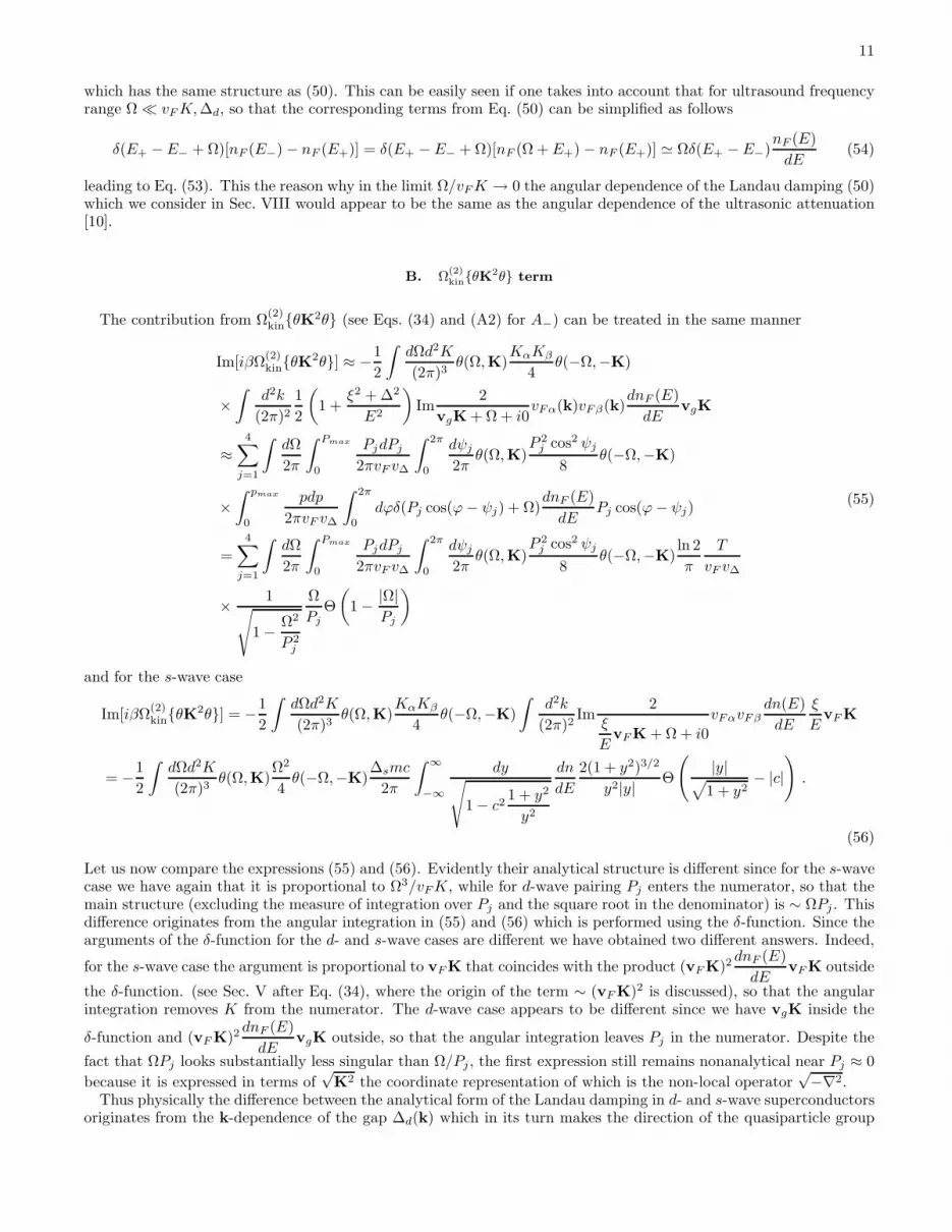
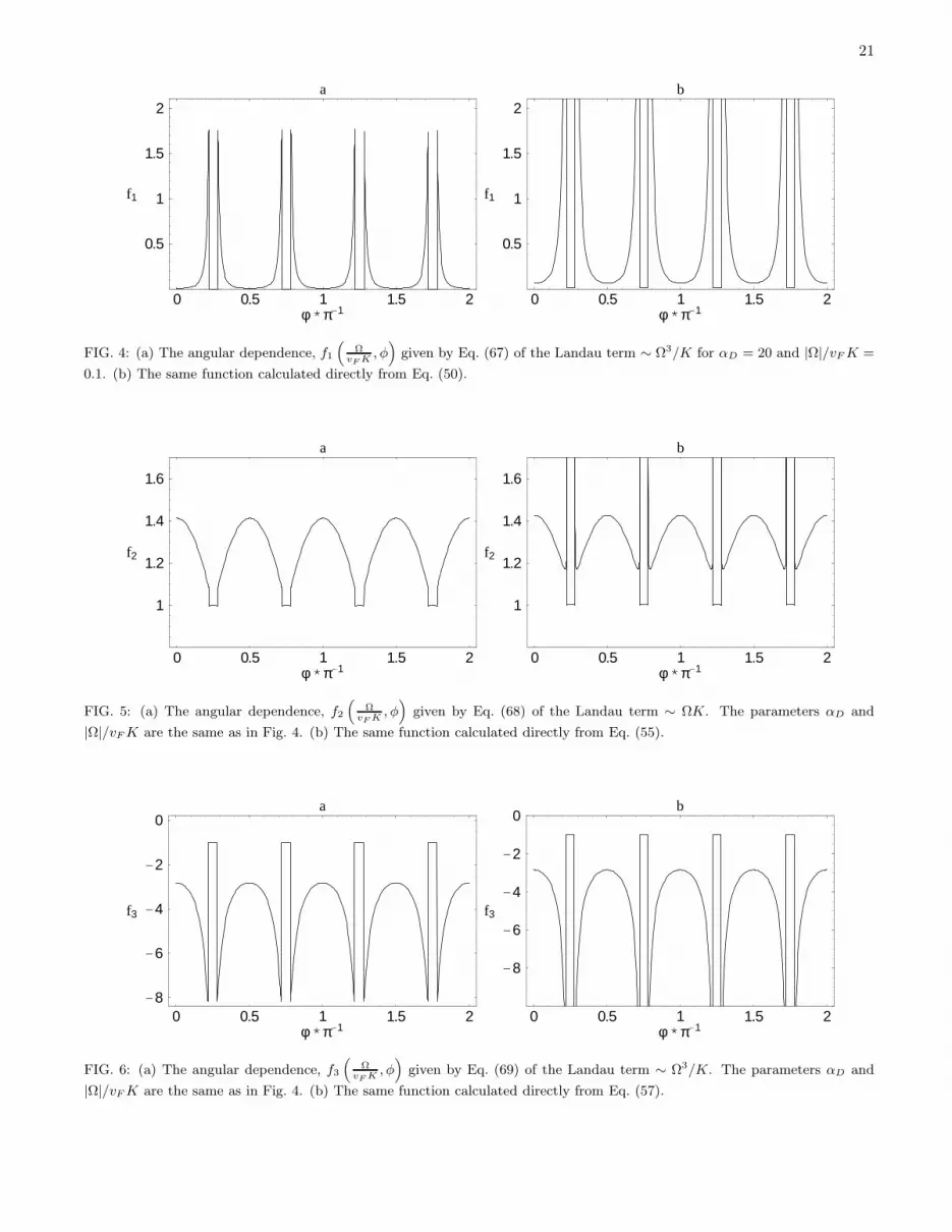
In Figs. 4 (a), 5 (a) and 6 (a) we show the functions f1, f2 and f3 which describe the intensity of Landau damping(f1 and f3 for the term ∼ Ω3/K and f2 for the term ∼ ΩK, respectively) as a function of the direction in the plane.Although the functions f1 and f3 describe the directional dependence for the same ∼ Ω3/K term, we do not combinethese functions into the single function because they originate from the different expressions. (We recall that f1originates from Eq. (50) and f3 originates from Eq. (57), respectively.) For the comparison in Figs. 4 (b), 5 (b) and6 (b) we show the directional dependences calculated by the direct substitution of Eq. (61) into Eqs. (50), (55) and(57) without making the approximations we just described. As one can see, the approximate representation (66),(67) - (69) despite its relatively simple form (we have used only the terms ∼ Ω3/K and ∼ ΩK) gives reasonablygood expression for the Landau damping terms. The biggest discrepancies are seen between Fig. 4 (a) and Fig. 4 (b)because more approximations were made to obtain f1 term.

As we mentioned in Sec. VII, the angular dependence described by f1 (see Fig. 4 (a)) coincides with the angulardependence of the ultrasonic attenuation [10] in the limit Ω/vFK → 0. Indeed the Θ-functions from (67) disappearwhen Ω/vFK → 0 and Eq. (67) reduces to the corresponding equation from [10].

We stress also that the analytical structure of the damping terms in (66) appears to be quite different from thedissipation introduced in [27] into the “phase only” action basing on the low frequency conductivity measurements.

Since f1 + 2f3 and f2 terms are odd functions of the frequency Ω, they integrate to zero in Ωkin. Nevertheless, thedamping terms are manifest in the equation of motion and in the propagator of the BKT mode which is consideredbelow.

Comparing Figs. 4, 5 and 6, one can see that the functions f1 and f3 have more pronounced angular dependencethan f2. Although as we explained above, the contribution from a given node is zero if for some K the condition (63)is not satisfied, this condition can still simultaneously be satisfied for the neighboring nodes, so that the sum over allnodes in f1 – f3 is not necessarily zero. We note also that by the absolute value both f1 (or f3) and f2 terms arepractically the same. This can be easily seen if we rewrite, for example, f1 term as

Ω3

K

ln 2

π

T

v∆v2F

f1

(

Ω

vFK,φ

)

= ΩK

(

Ω

vFK

)2ln 2

π

T

v∆f1

(

Ω

vFK,φ

)

≈ ΩKln 2

6

T

vFf1

(√

π

6αD, φ

)

, (70)

where writing the last identity we explicitly used the ratio Ω/vFK for the BKT mode at T = 0 given above.In such a way following [4] we can write an approximate propagator of the BKT mode near T = 0 as

DRθ (Ω,K) ≈

1

4a√πvF v∆

[

Ω2 −K2

(

πvF v∆6

− 2 ln 2avF

π

√αDT

)

+ 2iaγ(φ)TΩK

]−1

(71)

with

γ(φ) = ln 2

[

1

6

√

π

αD

(

f1

(√

π

6αD, φ

)

+ 2f3

(√

π

6αD, φ

))

+

√

αD

πf2

(√

π

6αD, φ

)]

. (72)

As discussed in [4] Eq. (71) has the form of a bosonic propagator with damping and its line-width has an explicit K

dependence. In contrast to the s-wave case, the width depends not only on the absolute value of |K|, but also on thedirection of K. The angular dependence for γ(φ) is shown in Fig. 7. Despite a simple form of the propagator (71),the corresponding effective wave operator (the transform of D−1

θ to space and time) has a nonlocal form in coordinatespace due to the presence of the damping term which depends [4] on |K|.

16

Comparing the second term in parentheses of (71) with the damping term one can see that they have the sameorder of magnitude showing that even for the low temperature region the Landau damping becomes important andits magnitude is comparable with term which describes the linear low temperature decrease in the superfluid stiffness.

We stress also the difference between the Landau damping representation in Eqs. (71) and (66). While the propa-gator (71) relies on the particular dispersion law for the BKT mode with the approximate v given by Eq. (43), ourEq. (66) along with Eqs. (67) - (69) present a rather general representation for the Landau damping terms derivationof which did not rely on any particular dispersion law for the phase excitations. Thus it can be, in principle, used todescribe the damping of the plasmons in charged superconductor. The only assumption we made is that Ω/vFK ≪ 1,which was used to derive more simple and transparent representation for the Landau damping. For the more generalcase one should use the results from Sec. VII.

IX. CONCLUDING REMARKS

It is very important to note that the collective phase excitations described by the propagator similar to (71) can andhave indeed been studied experimentally. Indeed the measurements of the order parameter dynamical structure factorin the dirty Al films allowed to extract the dispersion relation of the corresponding Carlson-Goldman mode and toinvestigate its temperature dependence [28]. It is important to stress that since the real systems are charged this modeappears to be different from the sound-like Bogolyubov-Anderson mode which exists in a neutral superfluid Fermiliquid. However, as discussed in [22] (see also [8] and Refs. therein) the discovery of Carlson-Goldman collective mode[28] overcame the widespread opinion that the Bogolyubov-Anderson collective oscillations predicted for a neutralsuperfluid should be forced to the frequencies on the order of the plasma frequency. It appears that if under certainconditions the frequency of the phase excitations is sufficiently low, the normal electron fluid may screen completelythe associated electric field, thereby making the theory of uncharged superconductor applicable [29]. The conditionsfor screening and occurrence of the Carlson-Goldman mode in s-wave superconductors are favorable only if the systemsare dirty (to suppress the Landau damping) and T . Tc [22]. As recently claimed in [8] in d-wave superconductors theconditions appear to much less strict, so that the Carlson-Goldman mode may be observed in the clean systems forT down to 0.2Tc. Now there are some new questions which would be interesting to address from both experimentaland theoretical points of view.First of all, there is a general question whether the Carlson-Goldman mode which is the equivalent of the Goldstonemode for the charged system can be observed experimentally. There are also a lot of theoretical questions which studywould make this kind of experiment possible. Leaving aside the specific of the Carlson-Goldman mode studied in [8]we mention some of them which are directly related to the present work.1. The Carlson-Goldman experiment [28] measures so called dynamical structure factor. This factor has a peakassociated with the phase excitations the width of which is primarily controlled by the Landau damping. Thereforeour result that the intensity of Landau damping has a strong directional dependence should be taken into accountin the calculation of the structure factor. In particular, the lowest for the observation of the Carlson-Goldman modetemperature 0.2Tc in [8] is obtained for the nodal direction. As can be seen from, for example, Fig.4 and 5, thecorresponding Landau damping terms become maximal in the vicinity of this direction which should likely result inwidening of the corresponding peak. If this widening is too big that the peak may become unobservable, this wouldagain suggest that the dirty samples should be used for the experiment.2. Taking into account the lattice effects and the dominance of the nodal excitations we have obtained that the velocityof the phase excitations at T → 0 is given by vlat = vF

√

π/6αD (see Eq. (43) and the discussion after Eq. (23)).

This expression appears to be quite different from the well-known continuum result, vcont = vF /√

2. The estimatesof the velocities vcont and vlat obtained from the values vF and αD [11] are presented in Table I. It is seen from theseestimates that the difference between the description proceeding from continuum and lattice models can be quitedifferent. However the estimates of the minimal for the observation of the Carlson-Goldman mode temperature in [8]

are based on the continuum expression vcont = vF /√

2. Thus it would be interesting to reconsider these estimates forthe lattice case.3. Finally, as pointed out in [9] if the plasmon is at finite frequency at K → 0, the Landau damping does not occursince when Ω is finite and K→ 0 it is impossible to satisfy Cerenkov condition discussed above. However, a very smallvalue of the plasma frequency in HTSC suggests that the Landau damping may still be relevant when K is nonzeroand the Cerenkov condition can be satisfied. Thus the corresponding damping terms should be included in the “phaseonly” actions which are used to describe plasma excitations in d-wave superconductors. Predicted anisotropy of theLandau damping would result in the damping anisotropy for the plasma excitations.

To summarize, we have considered the “phase only” effective action for so called neutral (or uncharged) fermionicsuperfluid with d- and s-wave pairing in 2D. When the damping terms are included into this action, it turns outnon-local in coordinate space and its analytical structure for the d-wave case is very different from the s-wave case.

17

To consider a charged superfluid it is necessary to combine the approaches used in the present paper and in [8, 9] toconsider the Landau damping in the presence of Coulomb interaction.

X. ACKNOWLEDGMENTS

We gratefully acknowledge Dr. E.V. Gorbar, Dr. M. Capezzali, Prof. V.E. Mkrtchyan and especially Prof.V.P. Gusynin for careful reading of the manuscript and valuable suggestions. We thank Prof. P. Martinoli andDr. X. Zotos for stimulating discussion and for bringing the papers [8, 28, 29] to our attention. S.G.Sh. is gratefulto the members of the Institut de Physique, Universite de Neuchatel for hospitality. This work was supported bythe research project 2000-061901.00/1 and by the SCOPES-project 7UKPJ062150.00/1 of the Swiss National ScienceFoundation. V.M.L. also thanks NATO grant CP/UN/19/C/2000/PO (Program OUTREACH) for partial supportand Centro de Fisica do Porto (Portugal) for hospitality.

APPENDIX A

Substituting (21) into (30) and (34), using the definitions for πij and Πij and evaluating the matrix traces for thediagonal terms we obtain

A± ≡[

Παβ00 (iΩn,K)

Π33(iΩn,K)

]

=

T

∞∑

l=−∞

∫

d2k

(2π)22[(iωl + iΩn)iωl + ξ(k −K/2)ξ(k + K/2)±∆(k−K/2)∆(k + K/2)]V±(k)

[(iωl + iΩn)2 − ξ2(k + K/2)−∆2(k + K/2)][(iωl)2 − ξ2(k−K/2)−∆2(k−K/2)],

V±(k) ≡[

vFα(k)vFβ(k), “+′′;1, “−′′ .

]

(A1)

Performing in (A1) the summation over Matsubara frequencies and simplifying the result we arrive at

A± =

−∫

d2k

(2π)2

1

2

(

1− ξ−ξ+ ±∆−∆+

E−E+

)[

1

E+ + E− + iΩn+

1

E+ + E− − iΩn

]

[1− nF (E−)− nF (E+)]

+1

2

(

1 +ξ−ξ+ ±∆−∆+

E−E+

)[

1

E+ − E− + iΩn+

1

E+ − E− − iΩn

]

[nF (E−)− nF (E+)]

V±(k) ,

(A2)

where ξ± ≡ ξ(k ±K/2), E± ≡ E(k ±K/2) and ∆± ≡ ∆(k ±K/2). The second term in Eq. (A2) can be furthersimplified if one notices that the term with 1/(E+−E−− iΩn) transforms into the term (−1)/(E+−E− + iΩn) whenk→ −k. Note that the A± terms do coincide with the corresponding terms in [4].

For the mixed term (35) one obtains

Πα03(iΩn,K) =

T

∞∑

l=−∞

∫

d2k

(2π)22[(iωl + iΩn)ξ(k −K/2) + ξ(k + K/2)iωl]vFα(k)

[(iωl + iΩn)2 − ξ2(k + K/2)−∆2(k + K/2)][(iωl)2 − ξ2(k−K/2)−∆2(k−K/2)]

=

∫

d2k

(2π)2

(

ξ+2E+

− ξ−2E−

)[

1

E+ + E− + iΩn− 1

E+ + E− − iΩn

]

[1− nF (E−)− nF (E+)]

+

(

ξ+2E+

+ξ−

2E−

)[

1

E+ − E− + iΩn− 1

E+ − E− − iΩn

]

[nF (E−)− nF (E+)]

vFα(k)

=

∫

d2k

(2π)2

ξ+E+

[

1

E+ + E− + iΩn− 1

E+ + E− − iΩn

]

[1− nF (E−)− nF (E+)]

+

(

ξ+E+

+ξ−E−

)

1

E+ − E− + iΩn[nF (E−)− nF (E+)]

vFα(k) .

(A3)

18

To get the last identity we again replaced k → −k and took into account that vF (k) also changes sign underthis transformation. One can also check that Πα

30(iΩn,K) = Πα03(iΩn,K). Eq. (A3) is also in agreement with the

corresponding term in [4] denoted as D.The first and second terms in (A2) and (A3) have a clear physical interpretation [24]. The first term gives the

contribution from “superfluid” electrons. The second term gives the contribution of the thermally excited quasipar-ticles (i.e. “normal” fluid component). The essential physical difference between the two terms is that the superfluidterm involves creation of two quasiparticles, with the minimum excitation energy in the s-wave case being 2∆s. (Forthe d-wave case the minimum energy turns out to be zero in the four nodal points, see the discussion at the end ofSec. VII.)

On the other hand, the normal fluid term involves scattering of the quasiparticles already present and the excitationenergy in this case can be arbitrary small, as in the normal metal, independently whether we are in the vicinity of thenode or not. Of course, the number of the quasiparticles participating in this scattering depends on the value of thegap and drastically increases if the gap is equal to zero in some points. As we shall see, the Landau damping termsoriginate from the second, normal fluid term. Note that our Eqs. (A2) and (A3) (as well as Eqs. (30), (34) and (35))are suitable for studying both s- and d-wave cases.

[1] E. Abrahams, T. Tsuneto, Phys. Rev. 152, 416 (1966).

[2] L.P. Gor’kov, Zh. Eksp. Teor. Fiz. 36, 1918 (1959) [Sov. Phys. JETP 9, 1364 (1959)].[3] I.J.R. Aitchison, D.J. Lee, Phys. Rev. B 56, 8303 (1997).[4] I.J.R. Aitchison, G. Metikas, D.J. Lee, Phys. Rev. B 62, 6638 (2000).[5] C.C. Tsuei, J.R. Kirtley, Rev. Mod. Phys. 72, 969 (2000).[6] A.C. Durst, P.A. Lee, Phys. Rev. B 62, 1270 (2000).[7] A.G. Sitenko, V.M. Mal’nev, Basics of plasma theory, Naukova Dumka, Kiev, 1994 (in Ukrainian) [English version, Plasma

physics theory, Chapman&Hall, London, 1995].[8] Y. Ohashi, S. Takada, Phys. Rev. B 62, 5971 (2000).[9] A. Paramekanti, M. Randeria, T.V. Ramakrishnan, S.S. Mandal, Phys. Rev. B 62, 6786 (2000).

[10] I. Vekhter, E.J. Nicol, J.P. Carbotte, Phys. Rev. B 59, 7123 (1999).[11] M. Chiao, R.W. Hill, C. Lupien, L. Taillefer, P. Lambert, R. Gagnon, P. Fournier, Phys. Rev. B 62, 3554 (2000).[12] H. Kleinert, Fortschritte der Physik 26, 565 (1978).[13] E.V.Gorbar, V.M. Loktev, V.S. Nikolaev Sverkhprovodimost’: Fiz., Khim., Tekhn. 7, 1 (1994) [Superconductivity: Physics,

Chemistry, Technology 7 , 1 (1994)].[14] Th. Meintrup, T. Schneider, H. Beck, Europhys. Lett. 31, 231 (1995).

[15] V.P. Gusynin, V.M. Loktev, and S.G. Sharapov, Pis’ma Zh. Eksp. Teor. Fiz. 65, 170 (1997) [JETP Lett. 65, 182 (1997)];

Zh. Eksp. Teor. Fiz. 115, 1243 (1999) [JETP 88, 685 (1999)].[16] V.M. Loktev, R.M. Quick and S.G. Sharapov, Phys. Rep. 349, 1 (2001).[17] We stress that this field is Grassmann variable since it satisfies the appropriate anti-commutation algebra (see Refs. in

[16]). The transformation (8) can be also regarded as a gauge transformation.[18] P. Ao, D.J. Thouless, X.-M. Zhu, Mod. Phys. Lett. B 9, 755 (1995); Preprint cond-mat/9312099.[19] O. Vafek, A. Melikyan, M. Franz, Z. Tesanovic, Phys. Rev. B 63, 134509 (2001).[20] S. De Palo, C. Castellani, C. Di Castro, B.K. Chakraverty, Phys. Rev. B 60, 564 (1999).[21] I.J.R. Aitchison, P. Ao, D.J. Thouless, X.-M. Zhu, Phys. Rev. B 51, 6531 (1995).[22] I.O. Kulik, O. Entin-Wolhman, R. Orbach, J. Low Temp. Phys. 43, 591 (1981).[23] R.M. Quick, S.G. Sharapov, Physica C 301, 262 (1998).[24] J.R. Schrieffer, Theory of Superconductivity, Benjamin, New York, 1964.[25] A.J. Leggett, Physica Fennica 8, 125 (1973).[26] It is the 2D analog of the well-known 3D Bogolyubov-Anderson-Goldstone mode [24]. The presence of this mode in 2D

does not imply that there is a breaking of the continuous symmetry in 2D (see, e.g. [15], V.P. Gusynin, V.M. Loktev, and

S.G. Sharapov, Pis’ma Zh. Eksp. Teor. Fiz. 69, 126 (1999) [JETP Lett. 69, 141 (1999)]; Zh. Eksp. Teor. Fiz. 117, 1143(2000) [JETP 90, 993 (2000)] and the detail in [16]) and U(1) symmetry remains in fact unbroken up to T ≡ 0.

[27] L. Benfatto, S. Carpara, C. Castellani, A. Paramekanti, M. Randeria, Phys. Rev. B 63, 174513 (2001).[28] R.V. Carlson, A.M. Goldman, Phys. Rev. Lett. 34, 11 (1975); F.E. Aspen, A.M. Goldman, J. Low Temp. Phys. 43, 559

(1981).[29] G. Brieskorn, M. Dinter, H. Schmidt, Solid State Commun. 15, 757 (1974).

19

TABLE I: The Fermi velocities vF and anisotropies of the Dirac spectrum, αD of YBa2Cu3O6.9 and Bi2Sr2CaCu2O8 at optimaldoping from [11]. The velocities of the phase excitations for the continuum, vcont and lattice, vlat limits at T = 0.

vF , ×107 cm/s αD vcont, ×107 sm/s vlat, ×106 sm/c

YBCO 2.5 14 1.77 4.8

BSCCO 2.5 19 1.77 4.2

=2

=2

=2

=2

k

y

k

x

K

BZ 1

BZ 2

BZ 3

BZ 4

FIG. 1: For µ = 0 the Fermi surface (dotted line) represents the points where ε(k) = −2t(cos kx+cos ky) = 0 (in the units wherethe lattice constant a = 1). There are four nodes centered at (±π/2,±π/2) around which the energy spectrum is linearized.The corresponding nodal sub-zones (see Eq. (25)) are called BZ j with j = 1, . . . , 4. For αD ≪ 1 the Landau damping developsonly if the direction of the phason momentum K is within one of the “cones”. The size of these cones is dependent on the ratioc = Ω/vF K, so that the cones shrink as |c| → 1 (see Eqs. (67) - (69)).

20

0 0.5 1 1.5 2∆d * t-1

0.25

0.5

0.75

1

1.25

1.5

1.75

v

FIG. 2: The dependence of the Goldstone mode velocity, v(T = 0) on the amplitude of the gap, ∆d. Solid line is the result ofnumerical calculation with ξ(k) = −2(cos kx +cos ky), ∆(k) = ∆d/2(cos kx − cos ky) (we put t = a = 1, so that ∆d is expressedin units of t). Thin line is obtained using Eq. (43). The anisotropy of the Dirac spectrum for this case is αD = 4/∆d, so that∆d = 0.2 corresponds to αD = 20.

K2

K1

K

k‘

1

k‘

2

FIG. 3: The directional dependence of the Landau damping for one node imposed by Θ

(

1 − |Ω|√v2

FK2

1+v2

∆K2

2

)

for αD = 2. For

a given Ω only excitations with the momenta K which are outside the ellipse (in the shaded region) can contribute into theLandau damping. For a fixed ratio |Ω|/vF |K| the presence of the Landau damping depends not only on |K|, but also on itsdirection. For example, for a vector having the length of the vector K shown in the figure the Landau damping is possible onlyif its direction is sufficiently close to the direction of k1 normal to the Fermi surface.

21

0 0.5 1 1.5 2φ*π-1

0.5

1

1.5

2

f1

a

0 0.5 1 1.5 2φ*π-1

0.5

1

1.5

2

f1

b

FIG. 4: (a) The angular dependence, f1

(

ΩvF K

, φ)

given by Eq. (67) of the Landau term ∼ Ω3/K for αD = 20 and |Ω|/vF K =

0.1. (b) The same function calculated directly from Eq. (50).

0 0.5 1 1.5 2φ*π-1

1

1.2

1.4

1.6

f2

a

0 0.5 1 1.5 2φ*π-1

1

1.2

1.4

1.6

f2

b

FIG. 5: (a) The angular dependence, f2

(

ΩvF K

, φ)

given by Eq. (68) of the Landau term ∼ ΩK. The parameters αD and

|Ω|/vF K are the same as in Fig. 4. (b) The same function calculated directly from Eq. (55).

0 0.5 1 1.5 2φ*π-1

-8

-6

-4

-2

0

f3

a

0 0.5 1 1.5 2φ*π-1

-8

-6

-4

-2

0

f3

b

FIG. 6: (a) The angular dependence, f3

(

ΩvF K

, φ)

given by Eq. (69) of the Landau term ∼ Ω3/K. The parameters αD and

|Ω|/vF K are the same as in Fig. 4. (b) The same function calculated directly from Eq. (57).

22

0 0.5 1 1.5 2φ*π-1

3

3.5

4

4.5

5

γ

FIG. 7: The angular dependence of the decay constant γ(

ΩvF K

, φ)

in θ-propagator (71) for αD = 20 and |Ω|/vF K =√

π

6αD≃

0.16.