MARINE ECOLOGY PROGRESS SERIESMar Ecol Prog Ser

Vol. 426: 71–86, 2011doi: 10.3354/meps09047

Published March 28

INTRODUCTION

Generally, nutrient-rich marine areas support classi-cal food chains with a broad autotrophic base domi-nated by large phytoplankton and copepods. In con-trast, oligotrophic waters, often strongly stratified, aredominated by small phytoplankton and high relativeheterotrophic biomasses (Gasol et al. 1997) and thefood web structure is more complex. However, suchgeneralizations may be challenged by specific hydro-

graphic features such as mesoscale eddies in the openoligotrophic oceans, which lead to extensive spatialvariability and intermittency in production and assem-blage structure of the plankton (Platt et al. 1989).Hence, such oceanic regions should not be consideredhomogeneous in space and constant in time.

The Sargasso Sea is an oligotrophic region in thewestern part of the North Atlantic Ocean surroundedby ocean currents. The biological system is influencedby complex patterns of thermal fronts (e.g. Voorhis &

© Inter-Research 2011 · www.int-res.com*Corresponding author. Email: tgin@aqua.dtu.dk(Second superscript numbers indicate present addresses)

Distribution and production of plankton communitiesin the subtropical convergence zone of the

Sargasso Sea. II. Protozooplankton and copepods

Nikolaj G. Andersen1, 4, Torkel Gissel Nielsen1, 2,*, Hans Henrik Jakobsen2,1, Peter Munk2, Lasse Riemann3, 4

1National Environmental Research Institute, Aarhus University, Department of Marine Ecology, 4000 Roskilde, Denmark2National Institute of Aquatic Resources, DTU Aqua Section for Oceanecology and Climate,

Technical University of Denmark, DTU Kavalergården 6, 2920 Charlottenlund, Denmark3Department of Natural Sciences, Linnaeus University, 39182 Kalmar, Sweden

4Marine Biological Section, University of Copenhagen, Strandpromenaden 5, 3000 Helsingør, Denmark

ABSTRACT: The oligotrophic Sargasso Sea in the western part of the North Atlantic Ocean is influ-enced by a complex set of oceanographic features that might introduce nutrients and enhance pro-ductivity in certain areas. To increase our understanding of the variability in plankton communitiesand to determine the potential reasons why Atlantic eels Anguilla spp. use this area for spawning, weinvestigated the distribution and productivity of the zooplankton community across the SubtropicalConvergence Zone (STCZ) in the Sargasso Sea in March and April 2007. The vertical and horizontaldistributions of protozoans and metazooplankton were investigated at 33 stations along 3 north tosouth transects ranging from 64 to 70° W to a depth of 400 m. Copepods dominated the metazoo-plankton, while heterotrophic athecate dinoflagellates dominated the protozoan biomass. Other im -portant groups were appendicularians, gastropod larvae and ostracods. Most of the recorded meta-zoan groups responded numerically to the frontal features (i.e. the surfacing of the isotherms) withhigh abundance in the STCZ compared with areas north and south of this. Juvenile copepod growthand egg production peaked in the STCZ, with a weight-specific growth rate of juvenile copepodsranging from 0.09 to 0.21 d–1, and a much lower specific egg production in the order of 0.01% d–1. TheSargasso Sea is described as oligotrophic, but the availability of athecate dinoflagellates and ciliatesin the STCZ potentially leads to an enhanced mesozooplankton secondary production, which may inturn be available to organisms at higher trophic levels such as larvae of Atlantic eels.

KEY WORDS: Sargasso Sea · Ciliates · Heterotrophic dinoflagellates · Copepods · Convergence zone

Resale or republication not permitted without written consent of the publisher

Mar Ecol Prog Ser 426: 71–86, 2011

Her sey 1964), irregular mesoscale eddies (McGilli -cuddy et al. 1998, Eden et al. 2009), advective transportof water masses (Palter et al. 2005) and a seasonal con-vective overturn (Hansell & Carlson 2001), all of theseleading to spatio-temporal variability in planktonicproductivity. While the Bermuda Atlantic Time-SeriesStudy (BATS) site is among the most intensively stud-ied marine sites in the world (Steinberg et al. 2001),data on horizontal and vertical variability in planktonbiomass, composition and productivity of the southernSargasso Sea is limited.

The subtropical convergence zone (STCZ) is a char-acteristic oceanographic feature that borders thesouthern part of the Sargasso Sea. There, cold watersfrom the north meet warm tropical waters from thesouth (Voorhis & Hersey 1964, Halliwell et al. 1994).Previous studies on abundance and distribution ofmeso zooplankton in the Sargasso Sea have focused onareas north of the STCZ (Deevey 1971, Deevey &Brooks 1971, Madin et al. 2001). Only a few studieshave covered the STCZ (Colton et al. 1975, Böttger1982), and these showed north to south differences inabundance and biomass in the mesozooplankton com-munities. However, in these studies the food web char-acteristics were not related to the physical characteris-tics of the STCZ, and in general the physical–biological linkages in this area are poorly understood.

The southern Sargasso Sea is the spawning site ofthe declining populations of Atlantic eels, the Ameri-can eel Anguilla rostrata and the European eel A. an -guilla, of which the European eel population is at a his-torical low level (ICES 2006). Consequently, there ismotivation for improved understanding of ecologicalprocesses that supports the early life of the Atlanticeels in this region (Munk et al. 2010). Early studiessuggested that the prey of eel larvae includes lar-vacean houses and zooplankton faecal pellets (Mochi -oka & Iwamizu 1996), but recent data suggest that thediet encompasses a wide range of plankton organisms,including gelatineous zooplankton and copepods (Rie-mann et al. 2010).

Copepods account for 75 to 87% of mesozooplanktonabundance in the upper 500 m of the Sargasso Sea(Böttger 1982). They primarily graze on microplankton(>20 μm) and to a lesser extent on nanoplankton(>2 μm) (Berggreen et al. 1988, Calbet & Landry 1999,Calbet et al. 2000). The protozoans therefore play aprominent role in oligotrophic seas, re-packaging theprimary producers dominated by picoplankton (2 to0.2 μm) into size parcels available for the copepods.Investigations near Bermuda show that the biomass ofciliates and dinoflagellates is comparable with otheroligotrophic areas (Lessard & Murrell 1996) and thatthe grazing by the microzooplankton of primary pro-ducers (i.e. <20 μm) is substantial (Lessard & Murrell

1998). However, as stated above, productivity in theBermuda area is not likely to be representative of con-ditions within the STCZ.

The aim of the present study was to investigate link-ages between plankton dynamics and the oceano-graphic features characteristic of the southern Sargas -so Sea. We hypothesized that the physical processes inthe STCZ enhance proto- and metazooplankton pro-duction and biomass in this zone. In an accompanyingpaper, we investigated the primary and secondary pro-duction of the phyto- and picoplankton (Riemann et al.2011, this volume).

MATERIALS AND METHODS

Study area. The investigation was conducted on boardthe Danish Navy surveillance frigate ‘F359 Vædderen’during the Danish Galathea 3 Expedition. Sampling tookplace from March 29 to April 10, 2007, in the SargassoSea. On 3 cross-frontal transects along the longitudes64° W, 67° W and 70° W, 33 stations were sampled (seeFig. 1 in Riemann et al. 2011, this volume). The verticaldistribution of salinity and temperature was measureddown to 400 m with a CTD (Seabird 9/11) equipped witha 12 Niskin bottle 30 l rosette sampler. In addition, theCTD was equipped with a fluorometer (SCUFA Turnerdesign). Water samples from 10, 30, 60, 100, 200 and400 m were taken at all stations. After collection, the water was kept dark and immediately brought toa temperature controlled laboratory container, where subsamples were taken for further analyses.

Protozoan biomass. Samples were collected from10 m depth and from the fluorescence maximum. Im -mediately after the CTD rosette was on deck, a 300 mlsample of seawater was fixed in acid Lugol’s solution(2% final concentration). Samples were stored in thedark at 5°C and analysed within 3 months. Protozoanswere en umerated and sized in 50 ml Utermöhl settlingchambers under an inverted microscope (Utermöhl1958). Samples were allowed to settle for 24 h beforemicro scopic examination. Cells were grouped into fam-ily, genera or species with the highest taxonomical res-olution possible. Groups were subdivided into 10 μmequivalent spherical diameter intervals and their vol-umes were estimated by means of appropriate morpho-logy-derived volume relationship equations. We did notaddress chloroplasts in dinoflagellates; other studies in-dicate that dinoflagellate chloroplast pigment markersare absent in oligotrophic waters and the apparentlyautotrophic dinoflagellates are phago trophic (Jeong etal. 2005, Schlüter et al. in press). We are thus confidentthat assigning heterotrophy to the athecate dinoflagel-lates of unknown trophy is a reasonable as sumption.Cellular carbon content was estimated from the generic

72

Andersen et al.: Plankton in the Sargasso Sea

protozoan-specific volume: carbon regression given byMenden-Deuer & Lessard (2000).

Protozoan secondary production. Maximal dailyclearance rates were calculated from the group spe-cific ‘volume:clearance’ equations by Hansen et al.(1997). We assumed maximal clearance (Cmax, bodyvolumes × 105 h–1) because the in situ chlorophyll a(chl a) concentration converted to carbon (carbon: chl a= 50, Malone et al. 1993) was below the empiricallydetermined Km (2 ppm = 240 μg C l–1) from Han sen etal. (1997) as follows:

for ciliates: logCmax = 1.491 – 0.23log(Pvol) (1)

for dinoflagellates: logCmax = 0.851 – 0.23log(Pvol) (2)

where Pvol is the cell volume (μm3). The rates were nor-malized to in situ temperature applying a Q10 factor of2.8 (Hansen et al. 1997). The ingestion was calculatedfrom the size-specific clearance rates and the concen-tration of potential food, i.e. chl a × 50. The protozoanproduction (P, μg C l–1 d–1) was estimated from theingestion (I) assuming a growth yield of 0.33 (Hansenet al. 1997):

P = I × 0.33 (3)

Metazooplankton abundance. Vertical distributionof metazooplankton >50 μm in size was investigated atTransects 1 and 3 with a MultiNet Midi (HYDRO-BIOS) with an aperture of 0.25 m2. The MultiNet con-sists of 5 nets allowing the investigation of 5 strata:0–50 m, 50–100 m, 100–200 m, 200–300 m and 300–400 m, and 0–75 m, 75–150 m, 150–200 m, 200–300 mand 300–400 m at Transects 1 and 3, respectively. TheMultiNet was lowered to 400 m and retrieved verti-cally at a speed of 10 m min–1. Samples were fixed in4% formalin and stored at 5°C. At Transect 2 and at2 stations along Transect 3, Stns 32 (70° W, 29° N) and33 (70° W, 30° N), the MultiNet was not applied, andintegrated abundance was only determined down to250 m. At these stations, a 45 μm plankton net with anopening of 14 cm, inserted inside a larger Mik-net, was

used. This small net was also used at 5 other MultiNetstations. This approach made it possible to comparethe efficiencies of the 2 nets, resulting in a factor of1.2 applied to the catches of the small plankton net.Abundance estimates at Stn 31 (28.0° N) were obtainedfrom only 3 strata instead of 5, owing to failure of theMultiNet at that station.

Copepod and appendicularian biomass. Biomasseswere calculated for 3 main groups: Paracalanus, Clau -so calanus and Calocalanus spp. (referred to as cala -noids), Oithona spp. and other copepods (referred toas others). During the identification and enumeration,the lengths of adults, copepodites and nauplii weremeasured for 10 (when possible) individuals of eachspecies or genera at each station. Biomass for appendi -cularians were calculated for Oikopleura spp. and Fri -til laria spp. (mean length ± SD = 254.3 ± 37 μm, n =172). Length–weight regressions representative ofspecies morphologically similar to those in the presentstudy were obtained from the literature (Table 1).

Copepod growth rate. Growth rates of the dominantcopepodites were measured at 10 stations by the artifi-cial cohort method (Tranter 1976, Kimmerer & McKin-non 1987). Copepodites were collected with a 50 μmWP-2 net. Two oblique hand tows were made verti-cally from ca. 30 m depth to the surface. The collectedcopepods were stored in an insulated tank containingsurface water and processed in the following way. Thesample was diluted with 50 μm filtered surface sea -water to obtain a concentration of ~7 to 8 l–1 and thensiphoned into a 10 l collapsible polyethylene watercontainer. A 200 μm sieve was lowered into the bucketleaving organisms >200 μm outside. Water from insideof the sieve was siphoned to another submerged160 μm sieve. The submerged 160 μm sieve was gentlylifted and lowered while running surface water wasadded to the bucket outside the sieve. In that manner,organisms <160 μm were flushed out of the bucket andthe water inside the sieve then contained only an arti-ficial cohort of copepodites between 160 and 200 μm(mainly Stages C1 to C3). The water in the bucket was

73

Length–weight regression Applied group Reference

W = 3.18 × 10–6 L3.331 (ng C + μm) Nauplii Berggreen et al. (1988)

lnW = 3.25 lnL – 19.65 (μg + μm) Weights and biomasses reported Paracalanus, Clausocalanus Chisholm & Roff (1990)here are room-equilibrated weights, i.e. dry weight × 1.06 and Calocalanus spp.

logW = 3.16 logL – 8.18 (μg + μm) Oithona spp. Hopcroft et al. (1998a)

lnW = 2.74 lnL – 16.41 (μg + μm) Other calanoid species Chisholm & Roff (1990)

lnW = 1.96 lnL – 11.64 (μg + μm) Other cyclopoid species Chisholm & Roff (1990)

lnW = 1.15 lnTL – 7.79 (μg C + μm) Harpacticoid species Satapoomin (1999)

logW = 2.455 logTL – 6.96 (μg C + μm) Larvacean community Jaspers et al. (2009)

Table 1. Length–weight regressions applied in the present study

Mar Ecol Prog Ser 426: 71–86, 2011

then adjusted to obtain a concentration of ~7 to 8 l–1.Then we took 7 samples of 1 l each. Three start sam-ples were concentrated on a 50 μm mesh, rinsed into a100 ml container and fixed in 4% buffered formalin.The last 4 samples were transferred to four 5 l plasticcontainers and 3 l of 50 μm filtered surface seawaterwas added. Before use, the plastic containers wererepeatedly filled with surface water and left on deckexposed to full sunlight to remove potential contami-nants. The containers were incubated under deck in a1 m3 plastic container with running surface water. Dur-ing the day the ship’s hatches provided light, and dimlight from the ship illuminated the containers at night.No attempt was made to reach a specific number ofcopepodites per container. After 24 h incubation, thesamples were concentrated on a 50 μm filter, checkedfor dead copepodites under a dissecting microscope(no mortality was observed) and fixed in 4% bufferedformalin. The incubation temperature for each experi-ment is the mean of the start and final temperature(Δmax, 2.2°C).

Prosome lengths (to articulation point with urosome)of the calanoids and Oithona spp. were measured witha stereo microscope (Olympus SZ40 Zoom) under 80×magnification. Up to 30 specimens of each taxon werecounted per sample. Damaged organisms were notconsidered. After the samples were processed thecopepodites were stored in 96% ethanol.

The fractionating process did not exclude particles<160 μm completely. Therefore, some nauplii couldhave metamorphosed into Stage C1 during incubationresulting in a lower calculated growth rate (Kimmereret al. 2007). To account for this, the amount of C1 in theincubated samples was adjusted to the abundance ofC1 in the start samples in cases with surplus C1 cope-podites. Lengths were converted to weights usinglength–weight regressions before calculation of meanweight. The weight-specific growth rate (μ) per daywas calculated as:

(4)

where T = incubation time in hours, W0 = mean weightat the start of the incubation, WT = mean weight at theend of the experiment.

Except for Paracalanus, Clausocalanus and Calo ca -la nus spp. at Stn 32, no significant differences inweight between the 3 start samples (Kruskal-Wallistest: p > 0.05) were observed. We calculated 4 growthrates from the 4 incubated samples at each stationusing the arithmetic mean of the 3 start samples as W0.The final growth rate at each station is a mean of the 4growth rates.

Copepod egg production. Copepod egg productionwas measured for Acartia sp. at 6 stations on each of

Transects 2 and 3. Acartia was chosen as indicator ofsecondary production (Kiørboe & Johansen 1986) be -cause Acartia’s egg production actually reflects thefood ingested during incubation (Tester & Turner1990). The copepods were sampled at the same timeand by the same method as the copepods for growthrate experiments but with a 200 μm WP-2 net. Adultfemale Acartia spp. were picked out with a large borepipette and added to 600 ml polycarbonate bottles with50 μm filtered surface seawater; 3 females were addedper bottle and 3 to 5 replicate bottles were taken ateach station. After 24 h incubation under the same con-ditions as the growth rate experiments, samples werefiltered through a 50 μm net and eggs and live anddead females were counted. Overall mortality was<10% and dead females were omitted from any furthercalculations. The specific egg production (SEP, % d–1)was calculated by:

SEP = EP × (Ce/Cf) (5)

where EP = no. eggs female–1 d–1, Ce = egg carbon con-tent, Cf = female carbon content. The carbon content ofthe eggs and females was estimated from the egg vol-ume and a conversion factor of 0.14 × 10–6 μg C μm–3

(Kiørboe et al. 1985), and the length–weight regres-sion in Berggreen et al. (1988), respectively.

Juvenile secondary production. The calculation of ju-venile secondary production was based on biomassesand growth rates for the relevant groups. Biomasseswere calculated for 5 assemblages (the cala noids andOithona spp. used in the growth rate experiments andthe rest of the calanoids, cyclopoids and harpacticoids)each divided into nauplii (Stages N1 to N6) and cope-podites (Stages C1 to C5) giving biomasses for 10groups. Growth rates for the calanoids and Oithonaspp. were used at stations where they were measured.

Where juvenile growth rate was not measured, themean values for the calanoids or Oithona spp. were ap -plied to the relevant biomasses. Where growth rates forboth groups where available the mean growth rate wasapplied to the rest of the juvenile copepods. Where onlygrowth rate for one of the groups was measured, amean of the measured growth rate and the overallmean of the other group (calanoids or Oithona) wasused. At stations where no growth rates were available,an overall mean for the calanoids and Oitho na spp. wasused. Juvenile growth rates were transformed to per-cent (see Eq. 6) before production calculations.

gj = eμ – 1 (6)

where gj = juvenile specific growth rate (d–1) and μ =specific growth rate (d–1).

Adult secondary production. The production ofadult copepods was calculated from adult biomasses ofcalanoids, Oithona spp. and the remaining calanoids,

μ = × ⎛⎝

⎞⎠24

0

/ lnTWW

T

74

Andersen et al.: Plankton in the Sargasso Sea

cyclopoids and harpacticoids. The specific egg produc-tion rates were applied to the relevant biomasses foreach station. At stations where no egg production wasavailable an overall mean was applied. Unidentifiedcopepods were for both juvenile and adult biomassesdivided proportionally to calanoids, cyclopoids andharpacticoids. At stations with missing biomass mea-surements no production was calculated. Total dailycopepod production was estimated as the product ofthe copepod biomass and the specific growth:

P = (gj × Bj) + (SEP × Ba) (7)

where P = daily production (mg C m–2 d–1), Bj = juve-nile copepod biomass (mg C m–2), gj = juvenile specificgrowth rate (d–1), SEP = specific egg production (% d–1)and Ba = adult biomass. When comparing the contribu-tion of juvenile growth to total copepod production, thecopepod production was calculated assuming commu-nity-specific egg production to be representative forgrowth rates of all copepod stages (Berggreen et al.1988).

Estimated secondary production. We compared ourmeasured copepod secondary production with esti-mates made from using the backward step-wise multi-ple linear regression model of Hirst & Bunker (2003),where the secondary production depends on the meantemperature in the upper 400 m (T, °C), the total inte-grated body weight (BW) for 0 to 400 m of the copepodpopulation (mg C m–2) and the integrated chl a concen-tration (Ca, mg chl a m–2). The general equation used is:

(8)

The factors a, b, c and d are covering ‘All data’ and notchanged according to the copepod category (adult,juvenile, broadcasters and egg-carrying copepods)(Table 4 in Hirst & Bunker 2003).

Clearance rate. Ingestion rates were calculated fromspecific growth rate in juveniles and specific egg pro-duction in adults assuming an ingestion growth yieldof 33%. That is, ingestion rate equals secondary pro-duction rate multiplied by 3 (Berggreen et al. 1988).Before calculating ingestion, juvenile specific growthrate was transformed to percent (Eq. 6). Weights for therelevant species are an overall mean for all stations.

Clearance rate (C) was subsequently calculated as:

(9)

where C = clearance rate (ml ind.–1 d–1), I = ingestionrate (μg C d–1) and FC = food concentration (μg C l–1).Juveniles were assumed to exploit phytoplankton andprotozoans, while the adults were as sumed to ingestprotozoans and phytoplankton >10 μm (data on chl afractions are presented in our companion paper, Rie-mann et al. 2011).

Carbon budgets. To summarize and compare thefood web structure and the carbon cycling of the differ-ent water masses, carbon budgets were preparedwithin water masses of comparable oceanographiccharacteristics: (1) stations in the warm water masses(>25°C) south of the front on Transect 1, (2) the STCZbetween the 2 fronts and (3) the stations north of thefronts. The values of the budget represent biomassesand production and were estimated by trapezoidalintegration of each discrete sampling depth down to400 m depth where values were set to 0.

RESULTS

Oceanography

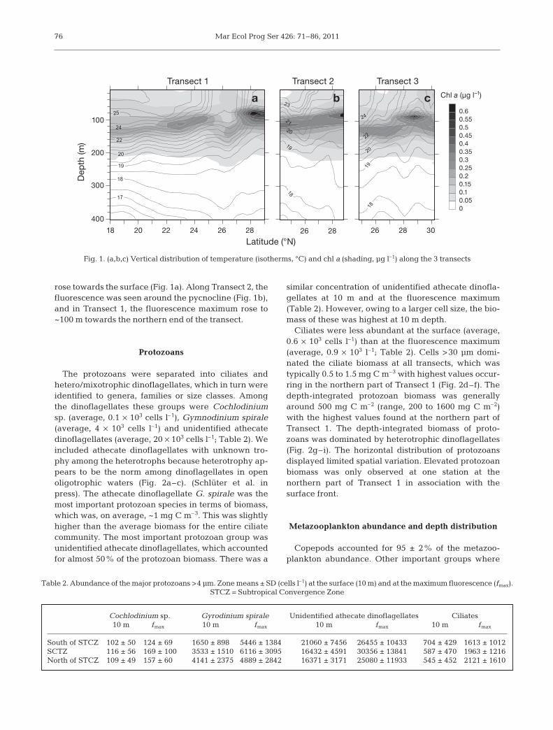
At the southern regions of all 3 transects the watercolumn was strongly stratified, in general with a ther -mo cline at ~150 m depth separating the warm surfacewater (27 to 21°C, south and north of the front, respec-tively) from colder subthermocline water (18 to 19°C)(Fig. 1a–c). Along Transect 1, the thermocline inclinedand isotherms from 75 to 125 m depth raised andformed a surface front. Further to the north, additionalsurfacing of isotherms was evident, resulting in a sec-ond front. North of this, the stratification of the watercolumn was weaker. We interpret these 2 fronts, andthe zone in between them as the STCZ. Transects 2 and3 were not of the same horizontal coverage and did notfully cover the southernmost front. Transect 2 was lo-cated right in the STCZ. Surface temperature changealong Transect 2 was only from 21 to 23°C (Fig. 1b). Thenorthernmost part of Transect 3 passed the northernedge of the STCZ (Fig. 1c). Salinity ranged from 36 to37 at all 3 transects (data not shown). At the southernsection of Transect 1, a salinity-stratified layer in the100 to 150 m strata was evident. From there, the salinitydeclined to 36 towards the surface and bottom. Thehalocline was less pronounced at the northern end ofthe transect, while at Transect 3, a halocline was onlyevident at the southernmost stations.

Chl a fluorescence

Distribution of chl a fluorescence was related to thephysical characteristics of the water column. At Tran-sects 1 and 2, a fluorescence maximum was located inthe pycnocline at ~125 m depth. Transect 3 also showedthis subsurface fluorescence peak, but the maximumwas located higher in the water column at the northern-most stations. A peak in the fluorescence at Transect 1was seen slightly higher in the water column, ~100 m,at the northern end of the transect where the isotherms

CI= ( ) ×

FC1000

log ( ) (log ) (log )10 10 10g a T b c C da= + + +BW

75

Mar Ecol Prog Ser 426: 71–86, 2011

rose towards the surface (Fig. 1a). Along Transect 2, thefluorescence was seen around the pycno cline (Fig. 1b),and in Transect 1, the fluorescence maximum rose to~100 m towards the northern end of the transect.

Protozoans

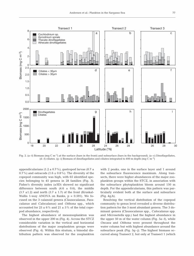
The protozoans were separated into ciliates and hetero/ mixotrophic dinoflagellates, which in turn wereidentified to genera, families or size classes. Amongthe dinoflagellates these groups were Cochlodiniumsp. (average, 0.1 × 103 cells l–1), Gymnodinium spirale(average, 4 × 103 cells l–1) and unidentified athecatedinoflagellates (average, 20 × 103 cells l–1; Table 2). Weincluded athecate dinoflagellates with unknown tro-phy among the heterotrophs because heterotrophy ap -pears to be the norm among dinoflagellates in openoligo trophic waters (Fig. 2a–c). (Schlüter et al. inpress). The athecate dinoflagellate G. spirale was themost important protozoan species in terms of biomass,which was, on average, ~1 mg C m–3. This was slightlyhigher than the average biomass for the entire ciliatecommunity. The most important protozoan group wasunidentified athecate dinoflagellates, which accountedfor almost 50% of the protozoan biomass. There was a

similar concentration of unidentified athecate dinofla-gellates at 10 m and at the fluorescence maximum(Table 2). However, owing to a larger cell size, the bio-mass of these was highest at 10 m depth.

Ciliates were less abundant at the surface (average,0.6 × 103 cells l–1) than at the fluorescence maximum(average, 0.9 × 103 l–1; Table 2). Cells >30 μm domi-nated the ciliate biomass at all transects, which wastypically 0.5 to 1.5 mg C m–3 with highest values occur-ring in the northern part of Transect 1 (Fig. 2d–f). Thedepth-integrated protozoan biomass was generallyaround 500 mg C m–2 (range, 200 to 1600 mg C m–2)with the highest values found at the northern part ofTransect 1. The depth-integrated biomass of proto-zoans was dominated by hetero trophic dinoflagellates(Fig. 2g–i). The horizontal distribution of protozoansdisplayed limited spatial variation. Elevated protozoanbiomass was only observed at one station at the northern part of Transect 1 in association with the surface front.

Metazooplankton abundance and depth distribution

Copepods accounted for 95 ± 2% of the metazoo-plankton abundance. Other important groups where

76

Cochlodinium sp. Gyrodinium spirale Unidentified athecate dinoflagellates Ciliates10 m fmax 10 m fmax 10 m fmax 10 m fmax

South of STCZ 102 ± 50 124 ± 69 1650 ± 898 5446 ± 1384 21060 ± 7456 26455 ± 10433 704 ± 429 1613 ± 1012SCTZ 116 ± 56 169 ± 100 3533 ± 1510 6116 ± 3095 16432 ± 4591 30356 ± 13841 587 ± 470 1963 ± 1216North of STCZ 109 ± 49 157 ± 60 4141 ± 2375 4889 ± 2842 16371 ± 3171 25080 ± 11933 545 ± 452 2121 ± 1610

Table 2. Abundance of the major protozoans >4 μm. Zone means ± SD (cells l–1) at the surface (10 m) and at the maximum fluorescence (fmax). STCZ = Subtropical Convergence Zone

0

0.05

0.1

0.15

0.2

0.25

0.3

0.35

0.4

0.45

0.5

0.55

0.6

Chl a (µg l–1)

400

300

200

100

18 20 22 24 26 28 26 28

Latitude (°N)

Transect 1 Transect 2 Transect 3D

ep

th (m

)

26 28 30

a b c

Fig. 1. (a,b,c) Vertical distribution of temperature (isotherms, °C) and chl a (shading, μg l–1) along the 3 transects

Andersen et al.: Plankton in the Sargasso Sea

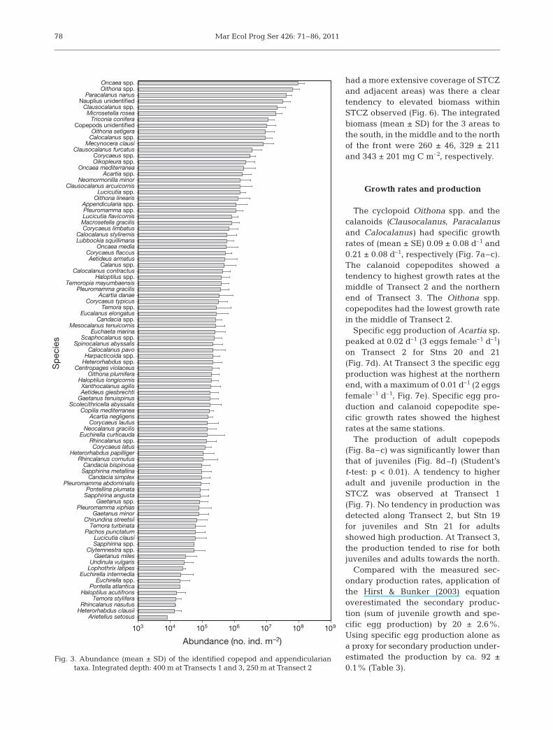
appendicularians (1.2 ± 0.7%), gastropod larvae (0.7 ±0.7%) and ostracods (1.6 ± 0.8%). The diversity of thecopepod community was high, with 65 identified spe-cies belonging to 45 genera in 28 families (Fig. 3).Fisher’s diversity index (±SD) showed no significantdifference between south (4.6 ± 0.6), the middle(3.7 ±1.2) and north (3.7 ± 1.7) of the front (Kruskal-Wallis 1-way ANOVA on Ranks, p = 0.591). We fo -cused on the 3 calanoid genera (Clausocala nus, Para-calanus and Calocalanus) and Oithona spp., whichaccounted for 25 ± 6% and 21 ± 5% of the total cope-pod abundance, respectively.

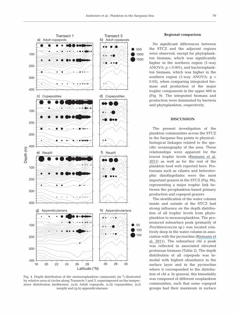
The highest abundance of mesozooplankton wasobserved in the upper 200 m (Fig. 4). Across the STCZconsiderable variation in the vertical and horizontaldistributions of the major zooplankton groups wereobserved (Fig. 4). Within this stratum, a bimodal dis-tribution pattern was ob served for the zooplankton

with 2 peaks, one in the surface layer and 1 aroundthe subsurface fluorescence maximum. Along tran-sects, there were higher abundances of the major zoo-plankton groups within the STCZ, in association withthe subsurface phytoplankton bloom around 150 mdepth. For the appendicularians, this pattern was par-ticularly evident both at the surface and subsurface(Fig. 4g,h).

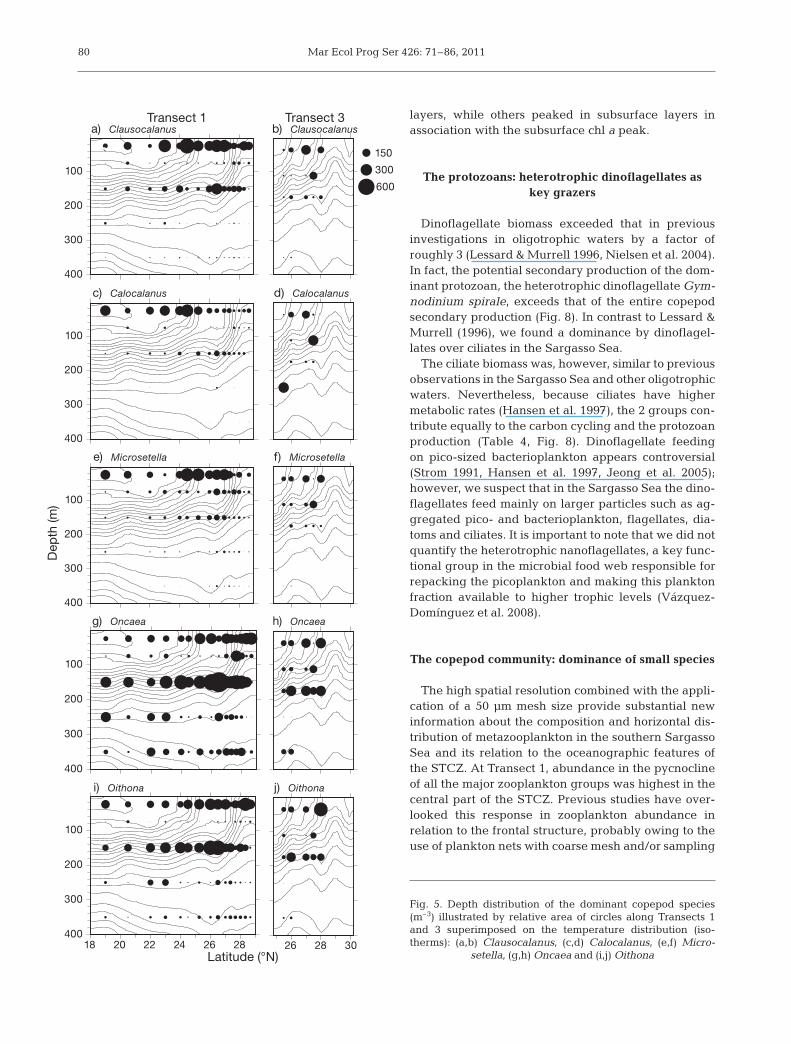
Resolving the vertical distribution of the copepodcommunity to genus level re vealed a diverse distribu-tion pattern for the 5 most abundant genera. The 3 do -minant genera (Clausocalanus spp., Calocalanus spp.and Microsetella spp.) had the highest abundance inthe upper 50 m of the water column (Fig. 5a–f), whileOncaea and Oi tho na were present throughout thewater column but with highest abundance around thesubsurface peak (Fig. 5g–j). The highest biomass oc -curred along Transect 2, but only at Transect 1 (which

77

Transect 3Transect 2Transect 1

2

0

4

6

8

Cochlodinium sp. Gyrodinium spiraleThecate dinoflagellatesAthecate dinoflagellates

0.5

0.0

1.0

1.5

2.0

2.5

Ciliates < 30µmCiliates > 30µm

a b c

d e f

18 20 22 24 26 280

500

1000

1500

2000DinoflagellatesCiliates

24 26 28

Latitude (°N)26 28 30

g h i

Bio

mass (m

g C

m–3)

Bio

mass (m

g C

m–2)

Fig. 2. (a–f) Biomass (mg C m–3) at the surface (bars in the front) and subsurface (bars in the background). (a–c) Dinoflagellates, (d–f) ciliates. (g–i) Biomass of dinoflagellates and ciliates integrated to 400 m depth (mg C m–2)

Mar Ecol Prog Ser 426: 71–86, 2011

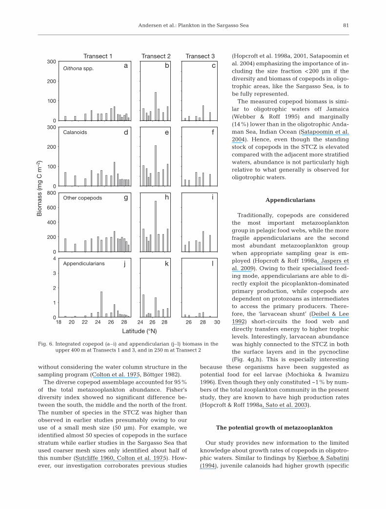
had a more extensive coverage of STCZand adjacent areas) was there a cleartendency to elevated biomass withinSTCZ ob served (Fig. 6). The integratedbiomass (mean ± SD) for the 3 areas tothe south, in the middle and to the northof the front were 260 ± 46, 329 ± 211and 343 ± 201 mg C m–2, respectively.

Growth rates and production

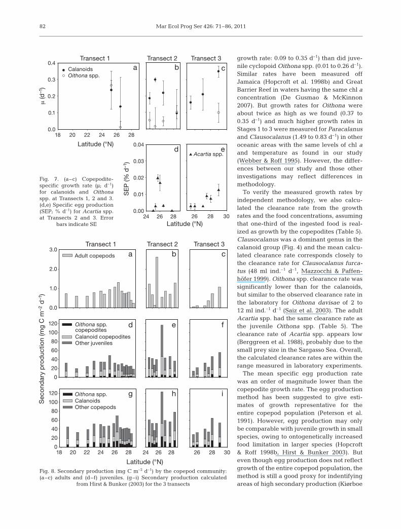
The cyclopoid Oithona spp. and thecala no ids (Clausocalanus, Paracalanusand Ca lo calanus) had specific growthrates of (mean ± SE) 0.09 ± 0.08 d–1 and0.21 ± 0.08 d–1, respectively (Fig. 7a– c).The calanoid copepodites showed atendency to highest growth rates at themiddle of Transect 2 and the northernend of Transect 3. The Oithona spp.copepodites had the lowest growth ratein the middle of Transect 2.

Specific egg production of Acartia sp.peaked at 0.02 d–1 (3 eggs female–1 d–1)on Transect 2 for Stns 20 and 21(Fig. 7d). At Transect 3 the specific eggproduction was highest at the northernend, with a maximum of 0.01 d–1 (2 eggsfemale–1 d–1, Fig. 7e). Specific egg pro-duction and calanoid copepodite spe-cific growth rates showed the highestrates at the same stations.

The production of adult copepods(Fig. 8a– c) was significantly lower thanthat of juveniles (Fig. 8d–f) (Student’st-test: p < 0.01). A tendency to higheradult and juvenile production in theSTCZ was observed at Transect 1(Fig. 7). No tendency in production wasdetected along Transect 2, but Stn 19for juveniles and Stn 21 for adultsshowed high production. At Transect 3,the production tended to rise for bothjuveniles and adults towards the north.

Compared with the measured sec-ondary production rates, application ofthe Hirst & Bunker (2003) equationoverestimated the secondary produc-tion (sum of juvenile growth and spe-cific egg production) by 20 ± 2.6%.Using specific egg production alone asa proxy for secondary production under -estimated the production by ca. 92 ±0.1% (Table 3).

78

Abundance (no. ind. m–2)

103 104 105 106 107 108 109

Sp

ecie

s

Arietellus setosusHeterorhabdus clausiiRhincalanus nasutus

Temora styliferaHaloptilus acutifrons

Pontella atlanticaEuchirella spp.

Euchirella intermediaLophothrix latipesUndinula vulgaris

Gaetanus milesClytemnestra spp.

Sapphirina spp.Lucicutia clausi

Pachos punctatumTemora turbinata

Chirundina streetsiiGaetanus minor

Pleuromamma xiphiasGaetanus spp.

Sapphirina angustaPontellina plumata

Pleuromamma abdominalisCandacia simplex

Sapphirina metallinaCandacia bispinosa

Rhincalanus cornutusHeterorhabdus papilliger

Corycaeus latusRhincalanus spp.

Euchirella curticaudaNeocalanus gracilis

Corycaeus lautusAcartia negligens

Copilia mediterraneaScolecithricella abyssalis

Gaetanus tenuispinusAetideus giesbrechtiXanthocalanus agilis

Haloptilus longicornisOithona plumifera

Centropages violaceusHeterorhabdus spp.Harpacticoida spp.

Calocalanus pavoSpinocalanus abyssalis

Scaphocalanus spp.Euchaeta marina

Mesocalanus tenuicornisCandacia spp.

Eucalanus elongatusTemora spp.

Corycaeus typicusAcartia danae

Pleuromamma gracilisTemoropia mayumbaensis

Haloptilus spp.Calocalanus contractus

Calanus spp.Aetideus armatus

Corycaeus flaccusOncaea media

Lubbockia squillimanaCalocalanus styliremis

Corycaeus limbatusMacrosetella gracilisLucicutia flavicornisPleuromamma spp.Appendicularia spp.

Oithona linearisLucicutia spp.

Clausocalanus arcuicornisNeomormonilla minor

Acartia spp.Oncaea mediterranea

Oikopleura spp.Corycaeus spp.

Clausocalanus furcatusMecynocera clausi

Calocalanus spp.Oithona setigera

Copepods unidentifiedTriconia conifera

Microsetella roseaClausocalanus spp.

Nauplius unidentifiedParacalanus nanus

Oithona spp.Oncaea spp.

Fig. 3. Abundance (mean ± SD) of the identified copepod and appendicularian taxa. Integrated depth: 400 m at Transects 1 and 3, 250 m at Transect 2

Andersen et al.: Plankton in the Sargasso Sea

Regional comparison

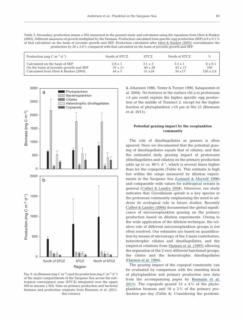
No significant differences betweenthe STCZ and the adjacent regionswere observed, except for phytoplank-ton biomass, which was significantlyhigher in the northern region (1-wayANOVA: p < 0.001), and bacterioplank-ton biomass, which was higher in thesouthern region (1-way ANOVA: p <0.05), when comparing integrated bio-mass and production of the majortrophic components in the upper 400 m(Fig. 9). The integrated biomass andproduction were dominated by bacteriaand phytoplankton, respectively.

DISCUSSION

The present investigation of theplankton communities across the STCZin the Sargasso Sea points to physical–biological linkages related to the spe-cific oceanography of the area. Theserelationships were apparent for thelowest trophic levels (Riemann et al.2011) as well as for the rest of theplankton food web reported here. Pro-tozoans such as ciliates and heterotro-phic dinoflagellates were the mostimportant grazers in the STCZ (Fig. 9b),representing a major trophic link be -tween the picoplankton-based primaryproduction and copepod grazers.

The stratification of the water columninside and outside of the STCZ hadstrong influence on the depth distribu-tion of all trophic levels from phyto-plankton to mesozooplankton. The pro-nounced subsurface peak (primarily ofProchlorococcus sp.) was located rela-tively deep in the water column in asso-ciation with the pycnocline (Riemann etal. 2011). The subsurface chl a peakwas reflected in associated elevatedprotozoan biomass (Table 2). The depthdistribution of all copepods was bi -modal with highest abundance in thesurface layer and in the pycnoclinewhere it corresponded to the distribu-tion of chl a. In general, this bimodalitywas composed of different zooplanktoncommunities, such that some copepodgroups had their maximum in surface

79

400

300

200

100

400

300

200

100

400

300

200

100

Dep

th (m

)

18 20 22 24 26 28

Latitude (°N)

400

300

200

100

26 28 30

a) Adult copepods

c) Copepodites

e) Nauplii

g) Appendicularians

500

1000

1500

50

100

150

b) Adult copepods

d) Copepodites

f) Nauplii

h) Appendicularians

Transect 1 Transect 3

Fig. 4. Depth distribution of the metazooplankton community (m–3) illustratedby relative area of circles along Transects 1 and 3, superimposed on the temper-ature distribution (isotherms). (a,b) Adult copepods, (c,d) copepodites, (e,f)

nauplii and (g,h) appendicularians

Mar Ecol Prog Ser 426: 71–86, 2011

layers, while others peaked in subsurface layers inassociation with the subsurface chl a peak.

The protozoans: heterotrophic dinoflagellates askey grazers

Dinoflagellate biomass exceeded that in previousinvestigations in oligotrophic waters by a factor ofroughly 3 (Lessard & Murrell 1996, Nielsen et al. 2004).In fact, the potential secondary production of the dom-inant protozoan, the heterotrophic dino flagellate Gym -no dinium spirale, ex ceeds that of the entire copepodsecond ary production (Fig. 8). In contrast to Les sard &Murrell (1996), we found a do mi nance by dinoflagel-lates over ciliates in the Sargasso Sea.

The ciliate biomass was, however, similar to previousobservations in the Sargasso Sea and other oligo trophicwaters. Nevertheless, because ciliates have highermeta bo lic rates (Hansen et al. 1997), the 2 groups con-tribute equally to the carbon cy cling and the protozoanproduction (Table 4, Fig. 8). Dinoflagellate feedingon pico-sized bacterioplankton appears controversial(Strom 1991, Hansen et al. 1997, Jeong et al. 2005);however, we suspect that in the Sargasso Sea the dino-flagellates feed mainly on larger particles such as ag -gre gated pico- and bacterioplankton, fla gel lates, dia-toms and ciliates. It is important to note that we did notquantify the heterotrophic nanoflagellates, a key func-tional group in the microbial food web responsible forrepacking the picoplankton and making this planktonfraction available to higher trophic levels (Vázquez-Domínguez et al. 2008).

The copepod community: dominance of small species

The high spatial resolution combined with the appli-cation of a 50 μm mesh size provide substantial newinformation about the composition and horizontal dis-tribution of metazooplankton in the southern SargassoSea and its relation to the oceanographic features ofthe STCZ. At Transect 1, abundance in the pycnoclineof all the major zooplankton groups was highest in thecentral part of the STCZ. Previous studies have over-looked this re sponse in zooplankton abundance inrelation to the frontal structure, probably ow ing to theuse of plankton nets with coarse mesh and/or sampling

80

400

300

200

100

400

300

200

100

400

300

200

100

18 20 22 24 26 28400

300

200

100

26 28 30

400

300

200

100

150

300

600

b) Clausocalanus

c) Calocalanus d) Calocalanus

e) Microsetella f) Microsetella

g) Oncaea

a) Clausocalanus

h) Oncaea

i) Oithona j) Oithona

Transect 1 Transect 3

Dep

th (m

)

Latitude (°N)

Fig. 5. Depth distribution of the dominant copepod species(m–3) illustrated by relative area of circles along Transects 1and 3 superimposed on the temperature distribution (iso -therms): (a,b) Clausocalanus, (c,d) Calocala nus, (e,f) Micro -

setella, (g,h) Oncaea and (i,j) Oithona

Andersen et al.: Plankton in the Sargasso Sea

without considering the water column structure in thesampling program (Colton et al. 1975, Böttger 1982).

The diverse copepod assemblage ac counted for 95%of the total metazooplankton abundance. Fisher’sdiversity index showed no significant difference be -tween the south, the middle and the north of the front.The number of species in the STCZ was higher thanob served in earlier studies presumably owing to ouruse of a small mesh size (50 μm). For example, weidentified almost 50 species of copepods in the surfacestratum while earlier studies in the Sargasso Sea thatused coarser mesh sizes only identified about half ofthis number (Sutcliffe 1960, Colton et al. 1975). How-ever, our investigation corroborates previous studies

(Hopcroft et al. 1998a, 2001, Sata poomin etal. 2004) emphasizing the importance of in -cluding the size fraction <200 μm if thediversity and biomass of copepods in oligo-trophic areas, like the Sargasso Sea, is tobe fully represented.

The measured copepod biomass is simi-lar to oligotrophic waters off Jamaica(Web ber & Roff 1995) and marginally(14%) lower than in the oligotrophic An da -man Sea, In dian Ocean (Satapoomin et al.2004). Hence, even though the standingstock of copepods in the STCZ is elevatedcompared with the adjacent more stratifiedwaters, abundance is not particularly highrelative to what generally is observed foroligotrophic waters.

Appendicularians

Traditionally, copepods are consideredthe most im portant metazooplanktongroup in pelagic food webs, while the morefragile appendicularians are the secondmost abundant metazooplankton groupwhen appropriate sampling gear is em -ployed (Hopcroft & Roff 1998a, Jaspers etal. 2009). Owing to their specialised feed-ing mode, appendicularians are able to di -rectly exploit the picoplankton-dominatedprimary production, while copepods aredependent on protozo ans as intermediatesto access the primary producers. There-fore, the ‘larvacean shunt’ (Deibel & Lee1992) short-circuits the food web anddirectly transfers energy to higher trophiclevels. Interestingly, larva cean abundancewas highly connected to the STCZ in boththe surface layers and in the pycnocline(Fig. 4g,h). This is especially interesting

because these organisms have been suggested aspotential food for eel larvae (Mochi oka & Iwamizu1996). Even though they only constituted ~1% by num-bers of the total zooplankton community in the presentstudy, they are known to have high production rates(Hopcroft & Roff 1998a, Sato et al. 2003).

The potential growth of metazooplankton

Our study provides new information to the limitedknowledge about growth rates of copepods in oligotro-phic waters. Similar to findings by Kiørboe & Sabatini(1994), juvenile calanoids had higher growth (specific

81

0

200

400

600

800Other copepods

0

100

200

300

Oithona spp. a b c

0

100

200

300Calanoids e fd

hg i

18 20 22 24 26 280

1

2

3

4Appendicularians

24 26 28 26 28 30

j k l

Transect 1 Transect 3 Transect 2

Latitude (°N)

Bio

mass (m

g C

m–2)

Fig. 6. Integrated copepod (a–i) and appendicularian (j–l) biomass in the upper 400 m at Transects 1 and 3, and in 250 m at Transect 2

Mar Ecol Prog Ser 426: 71–86, 2011

growth rate: 0.09 to 0.35 d–1) than did juve-nile cyclo poid Oithona spp. (0.01 to 0.26 d–1).Similar rates have been measured offJamaica (Hopcroft et al. 1998b) and GreatBarrier Reef in waters having the same chl aconcentration (De Gusmao & McKinnon2007). But growth rates for Oithona wereabout twice as high as we found (0.37 to0.35 d–1) and much higher growth rates inStages 1 to 3 were measured for Paracalanusand Clausocalanus (1.49 to 0.83 d–1) in otheroceanic areas with the same levels of chl aand temperature as found in our study(Webber & Roff 1995). However, the differ-ences between our study and those otherinvestigations may reflect differences inmethodology.

To verify the measured growth rates byindependent methodology, we also calcu-lated the clearance rate from the growthrates and the food concentrations, assumingthat one-third of the ingested food is real-ized as growth by the copepodites (Table 5).Clausocalanus was a dominant genus in thecalanoid group (Fig. 4) and the mean calcu-lated clearance rate corresponds closely tothe clearance rate for Clausocalanus furca-tus (48 ml ind.–1 d–1, Mazzocchi & Paffen-höfer 1999). Oi tho na spp. clearance rate wassignificantly lower than for the calanoids,but similar to the observed clearance rate inthe laboratory for Oithona davisae of 2 to12 ml ind.–1 d–1 (Saiz et al. 2003). The adultAcartia spp. had the same clearance rate asthe juvenile Oithona spp. (Table 5). Theclearance rate of Acartia spp. appears low(Berggreen et al. 1988), probably due to thesmall prey size in the Sargasso Sea. Overall,the calculated clearance rates are within therange measured in laboratory experiments.

The mean specific egg production ratewas an order of magnitude lower than thecopepodite growth rate. The egg productionmethod has been suggested to give esti-mates of growth representative for theentire copepod population (Peterson et al.1991). However, egg production may onlybe comparable with juvenile growth in smallspecies, owing to ontogenetically increasedfood limitation in larger species (Hopcroft& Roff 1998b, Hirst & Bunker 2003). Buteven though egg production does not reflectgrowth of the entire copepod population, themethod is still a good proxy for indentifyingareas of high secondary production (Kiørboe

82

18 20 22 24 26 280.0

0.1

0.2

0.3

0.4CalanoidsOithona spp.

24 26 280.00

0.01

0.02

0.03

0.04

Acartia spp.

26 28 30

a b c

d e

Transect 1 Transect 3 Transect 2

Latitude (°N)

Latitude (°N)

μ (d

–1)

SE

P (%

d–1

)

Fig. 7. (a–c) Copepodite-specific growth rate (μ; d–1)for calanoids and Oithonaspp. at Transects 1, 2 and 3.(d,e) Specific egg production(SEP; % d–1) for Acartia spp.at Transects 2 and 3. Error

bars indicate SE

0.0

1.0

2.0

3.0Adult copepods

0

20

40

60

80

100

120 Oithona spp. copepodites Calanoid copepoditesOther juveniles

0

20

40

60

80

100

120 Oithona spp. Calanoids Other copepods

a b c

e fd

hg i

18 20 22 24 26 28 24 26 28 26 28 30

Transect 1 Transect 3 Transect 2

Latitude (°N)

Seco

nd

ary

pro

du

ctio

n (m

g C

m–2 d

–1)

Fig. 8. Secondary production (mg C m–2 d–1) by the copepod community:(a–c) adults and (d–f) juveniles. (g–i) Secondary production calculated

from Hirst & Bunker (2003) for the 3 transects

Andersen et al.: Plankton in the Sargasso Sea

& Johansen 1986, Tester & Turner 1990, Sata poomin etal. 2004). No features in the surface chl a or protozoans>4 μm could explain the higher specific egg produc-tion at the middle of Transect 2, except for the higherfraction of phytoplankton >10 μm at Stn 21 (Riemannet al. 2011).

Potential grazing impact by the zooplankton community

The role of dinoflagellates as grazers is oftenignored. Here we documented that the potential graz-ing of dinoflagellates equals that of ciliates, and thatthe estimated daily grazing impact of protozoans(dinoflagellates and ciliates) on the primary productionadds up to ca. 86% d–1, which is several times higherthan for the copepods (Table 4). This estimate is highbut within the range measured by dilution experi-ments in the Sargasso Sea (Lessard & Murrell 1996)and comparable with values for subtropical oceans ingeneral (Calbet & Landry 2004). Moreover, our studyindicates that Gyrodinium spirale is a key species inthe protozoan community em phasising the need to ad -dress its ecological role in future studies. Recently Calbet & Landry (2004) documented the global signifi-cance of microzooplankton grazing on the primaryproduction based on dilution experiments. Owing tothe wide application of the dilution technique, the rel-ative role of different microzooplankton groups is notoften resolved. Our estimates are based on quantifica-tion by means of microscopy of the 2 main contributors,heterotrophic ciliates and dinoflagellates, and theempirical relations from Hansen et al. (1997) allowingthe separation of the 2 very different functional groups,the cilates and the heterotrophic dinoflagellates(Hansen et al. 1994).

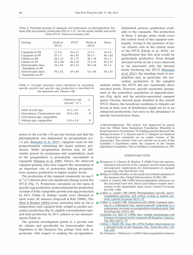
The grazing impact of the copepod community canbe evaluated by comparison with the standing stockof phytoplankton and primary production (see datafrom the accompanying paper by Riemann et al.2011). The copepods grazed 15 ± 4% of the phyto-plankton biomass and 18 ± 2% of the primary pro-duction per day (Table 4). Considering the predomi-

83

Production (mg C m–2 d–1) South of STCZ STCZ North of STCZ %

Calculated on the basis of SEP 2.9 ± 1 3.1 ± 3 3.3 ± 1 8 ± 0.1On the basis of juvenile growth and SEP 37 ± 11 40 ± 28 43 ± 17 100Calculated from Hirst & Bunker (2003) 44 ± 7 51 ±24 54 ±17 120 ± 2.6

Table 3. Secondary production (mean ± SD) measured in the present study and calculated using the equations from Hirst & Bunker(2003). Different measures of growth multiplied by the biomass. Production calculated from specific egg production (SEP) is 8 ± 0.1%of that calculated on the basis of juvenile growth and SEP. Production calculated after Hirst & Bunker (2003) overestimates the

production by 20 ± 2.6% compared with that calculated on the basis of juvenile growth and SEP

Bio

mass (m

g C

m–2)

0

500

1000

1500

2000

2500

3000PhytoplanktonBacterioplanktonCiliatesHeterotrophic dinoflagellatesCopepods

Region

South of STCZ STCZ North of STCZ

Pro

du

ctio

n (m

g C

m–2 d

–1)

0

500

1000

1500

2000

a

b

Fig. 9. (a) Biomass (mg C m–2) and (b) production (mg C m–2 d–1)of the major compartments of the Sargasso Sea across the sub-tropical convergence zone (STCZ) integrated over the upper400 m (means ± SD). Data on primary production and bacterialbiomass and production originate from Riemann et al. (2011,

this volume)

Mar Ecol Prog Ser 426: 71–86, 2011

nance of chl a in the <10 μm size fraction and that thephytoplankton was dominated by picoplankton (i.e.<2 μm, Riemann et al. 2011), copepods must be dis-proportionately consuming the larger primary pro-ducers. While picoplankton detritus may be effi-ciently grazed by protozoans and zooplankton, mostof the picoplankton is presumably unavailable tocopepods (Hansen et al. 1994). Hence, the observedcopepod grazing rates may support the assumption ofan important role of protozoans linking picoplank-tonic primary production to higher trophic levels.

The production of the copepod community (in mg Cm–2 d–1) did not show any significant change across theSTCZ (Fig. 7). Production calculated on the basis ofspecific egg production underestimated the productionon basis of both copepodite growth and egg productionby 92% (Table 3). Similar results were obtained inopen water off Jamaica (Hopcroft & Roff 1998b). TheHirst & Bunker (2003) proxy, including data on chl a,temperature and copepod body weight to predict sec-ondary production (Eq. 8), slightly overestimated cope-pod total production by 20% relative to our measure-ments (Table 3).

The present investigation points to a pivotal rolefor ciliates and specifically for heterotrophic dino -flagellates in the Sargasso Sea pelagic food web, inpar ticular with respect to making the picoplankton-

dominated primary production avail-able to the copepods. The productionof these 2 groups alone could coverthe carbon need of the copepod com-munity. Owing to the presence of lar-val Atlantic eels in the central areasof the STCZ (Munk et al. 2010), wehypothesized that this area would beparticularly productive. Even thoughelevated levels of chl a were observedto be associated with the thermalfronts bordering the STCZ (Riemannet al. 2011), the standing stock of zoo-plankton and, in particular, the sec-ondary production at the sampled

stations within the STCZ did not consistently showelevated levels. However, specific taxonomic groups,such as the subsurface population of appendiculari-ans (Fig. 4g,h) and the particle-associated copepodgenus Oncaea, showed peak densities in the centralSTCZ. Hence, the beneficial conditions to Atlantic eellarvae in their area of distribution might not lie in anenhanced productivity, but more in the abundance ofspecific favoured prey items.

Acknowledgements. The project was supported by grantsfrom the Villum Kann Rasmussen Foundation, Elisabeth &Knud Petersen’s Foundation, TK Holding and the Rod and Netfishing Licensee. P. J. Hansen and H. U. Riisgård are thankedfor constructive comments on an earlier version of the manuscript. The present work was carried out as part of theGalathea 3 Expedition under the auspices of the Danish Expedition Foundation. This is Galathea 3 contribution no. P76.

LITERATURE CITED

Berggreen U, Hansen B, Kiørboe T (1988) Food size spectra,ingestion and growth of the copepod Acartia tonsa duringdevelopment: implications for determination of copepodproduction. Mar Biol 99:341–352

Böttger R (1982) Studies on the small invertebrate plankton ofthe Sargasso Sea. Helgol Meeresunters 35:369–383

Calbet A, Landry MR (1999) Mesozooplankton influences onthe microbial food web: Direct and indirect trophic inter-actions in the oligotrophic open ocean. Limnol Oceanogr44:1370–1380

Calbet A, Landry MR (2004) Phytoplankton growth, micro-zooplankton grazing, and carbon cycling in marine sys-tems. Limnol Oceanogr 49:51–57

Calbet A, Landry MR, Scheinberg RD (2000) Copepod graz-ing in a subtropical bay: species-specific responses to amidsummer increase in nanoplankton standing stock. MarEcol Prog Ser 193:75–84

Chisholm LA, Roff JC (1990) Size–weight relationships andbiomass of tropical neritic copepods off Kingston, Jamaica.Mar Biol 106:71–77

Colton J, Smith DE, Jossi JW (1975) Further observations ona thermal front in the Sargasso Sea. Deep-Sea Res I 22:433–439

De Gusmao L, McKinnon A (2007) Mesozooplankton biomass

84

Grazing South of STCZ North of MeanSTCZ STCZ

Copepods on PB 17 ± 4 16 ± 11 15 ± 7 16 ± 8Copepods on PP 27 ± 7 56 ± 91 20 ± 1 40 ± 63Ciliates on PB 29 ± 15 37 ± 17 36 ± 18 34 ± 3Ciliates on PP 63 ± 241 36 ± 16 31 ± 20 43 ± 17Heterotrophic dino- 34 ± 20 36 ± 15 36 ± 18 34 ± 2flagellates on PB

Heterotrophic dino- 78 ± 43 47± 40 42 ± 46 56 ± 20flagellates on PP

Table 4. Potential grazing of copepods and protozoans on phytoplankton bio-mass (PB) and primary production (PP) in % d–1 for the south, middle and north

of the STCZ. Values are means ± SD

Clearance rate n(ml ind.–1 d–1)

Adult Acartia spp. 15.1 ± 0.7 11Paracalanus, Clausocalanus and 57.9 ± 9.0 9Calocalanus spp. copepoditesOithona spp. copepodites 15.6 ± 5.6 8

Table 5. Average clearance rates calculated by assumingspecific growth and specific egg production is one-third of

the ingestion rate. Means ± SD

Andersen et al.: Plankton in the Sargasso Sea

and copepod growth rates in the Whitsunday Islands,Great Barrier Reef, Australia. 4th Int Zooplankton Produc-tion Symp, Hiroshima, Japan, 28 May–1 Jun 2007

Deevey GB (1971) The annual cycle in quantity and composi-tion of the zooplankton of the Sargasso Sea off Bermuda.1. The upper 500 m. Limnol Oceanogr 16:219–240

Deevey GB, Brooks AL (1971) The annual cycle in quantityand composition of the zooplankton of the Sargasso Seaoff Bermuda. II. The surface to 2000 m. Limnol Oceanogr16: 927–943

Deibel D, Lee SH (1992) Retention efficiency of submicro -meter particles by the pharyngeal filter of the pelagic tuni-cate Oikopleura vanhoeffeni. Mar Ecol Prog Ser 81:25–30

Eden BR, Steinberg DK, Goldthwait SA, M cGillicuddy D J(2009) Zooplankton community structure in a cyclonic andmode-water eddy in the Sargasso Sea. Deep-Sea Res I 56:1757–1776

Gasol JM, del Giorgio PA, Duarte CM (1997) Biomass distrib-ution in marine planktonic communities. Limnol Oceanogr42: 1353–1363

Halliwell GR, Peng G, Olson DB (1994) Stability of the Sar-gasso Sea Subtropical Frontal Zone. J Phys Oceanogr 24:1166–1183

Hansell DA, Carlson CA (2001) Biogeochemistry of totalorganic carbon and nitrogen in the Sargasso Sea: controlby convective overturn. Deep-Sea Res II 48:1649–1667

Hansen B, Bjørnsen PK, Hansen PJ (1994) The size ratio be -tween planktonic predators and their prey. LimnolOceanogr 39:395–403

Hansen PJ, Bjørnsen PK, Hansen BW (1997) Zooplanktongrazing and growth: scaling within the 2–2,000 μm bodysize range. Limnol Oceanogr 42:687–704

Hirst AG, Bunker AJ (2003) Growth of marine planktoniccopepods: global rates and patterns in relation to chloro-phyll a, temperature, and body weight. Limnol Oceanogr48: 1988–2010

Hopcroft RR, Roff JC (1998a) Production of tropical appendic-ularians in Kingston Harbour, Jamaica: Are we ignoringan important secondary producer? J Plankton Res 20:557–569

Hopcroft RR, Roff JC (1998b) Zooplankton growth rates: theinfluence of female size and resources on egg productionof tropical marine copepods. Mar Biol 132:79–86

Hopcroft RR, Roff JC, Lombard D (1998a) Production of tropi-cal copepods in Kingston Harbour, Jamaica: the impor-tance of small species. Mar Biol 130:593–604

Hopcroft RR, Roff JC, Webber MK, Witt JDS (1998b) Zoo-plankton growth rates: the influence of size and resourcesin tropical marine copepodites. Mar Biol 132:67–77

Hopcroft RR, Chavez FP, Roff JC (2001) Size paradigms incopepod communities: a re-examination. Hydrobiologia453/454:133–141

ICES (2006) Reports of the Eifac/ICES Working Group onEels, Rome, Italy. International Council for Explorationof the Sea, Copenhagen, ICES CM 2006/ACFM 16, Ref.DFC, LRC, RMC: 101

Jaspers C, Nielsen TG, Carstensen J, Hopcroft RR, Møller EF(2009) Metazooplankton distribution across the SouthernIndian Ocean with emphasis on the role of larvaceans. JPlankton Res 31:525–540

Jeong HJ, Du Yoo Y, Park JY, Song JY and others (2005)Feeding by phototrophic red-tide dinoflagellates: five spe-cies newly revealed and six species previously known tobe mixotrophic. Aquat Microb Ecol 40:133–150

Kimmerer WJ, McKinnon AD (1987) Growth, mortality, andsecondary production of the copepod Acartia tranteri inWesternport Bay, Australia. Limnol Oceanogr 32:14–28

Kimmerer WJ, Hirst AG, Hopcroft RR, McKinnon AD (2007)Estimating juvenile copepod growth rates: corrections,inter-comparisons and recommendations. Mar Ecol ProgSer 336:187–202

Kiørboe T, Johansen K (1986) Studies of a larval herring (Clu-pea harengus L.) patch in the Buchan area. 4. Zooplanktondistribution and productivity in relation to hydrographicfeatures. Dana 6:37–51

Kiørboe T, Sabatini M (1994) Reproductive and life cyclestrategies in egg-carrying cyclopoid and free-spawningcalanoid copepods. J Plankton Res 16:1353–1366

Kiørboe T, Møhlenberg F, Hamburger K (1985) Bioenergeticsof the planktonic copepod Acartia tonsa: relation be -tween feeding, egg production and respiration, and com-position of specific dynamic action. Mar Ecol Prog Ser 26:85–97

Lessard EJ, Murrell MC (1996) Distribution, abundance andsize composition of heterotrophic dinoflagellates and cili-ates in the Sargasso Sea near Bermuda. Deep-Sea Res I43: 1045–1065

Lessard EJ, Murrell MC (1998) Microzooplankton herbivoryand phytoplankton growth in the northwestern SargassoSea. Aquat Microb Ecol 16:173–188

Madin LP, Horgan EF, Steinberg DK (2001) Zooplankton atthe Bermuda Atlantic Time-series Study (BATS) station:diel, seasonal and interannual variation in biomass,19941998. Deep-Sea Res II 48:2063–2082

Malone TC, Pike SE, Conley DJ (1993) Transient variations inphytoplankton productivity at the JGOFS Bermuda timeseries station. Deep-Sea Res II 40:903–924

Mazzocchi M, Paffenhöfer G (1999) Swimming and feedingbehaviour of the planktonic copepod Clausocalanus furca-tus. J Plankton Res 21:1501–1518

McGillicuddy DJ Jr, Robinson AR, Siegel DA, Jannasch HWand others (1998) Influence of mesoscale eddies on newproduction in the Sargasso Sea. Nature 394:263–266

Menden-Deuer S, Lessard EJ (2000) Carbon to volume rela-tionships for dinoflagellates, diatoms, and other protistplankton. Limnol Oceanogr 45:569–579

Mochioka N, Iwamizu M (1996) Diet of anguilloid larvae: lep-tocephali feed selectively on larvacean houses and fecalpellets. Mar Biol 125:447–452

Munk P, Maes GE, Hansen MM, Nielsen TG and others(2010) Oceanic fronts in the Sargasso Sea control the earlylife and drift of Atlantic eels. Proc R Soc B Biol Sci 277:3593–3599

Nielsen TG, Bjørnsen PK, Boonruang P, Fryd M and others(2004) Hydrography, bacteria and protist communitiesacross the continental shelf and shelf slope of theAndaman Sea (NE Indian Ocean). Mar Ecol Prog Ser 274:69–86

Palter JB, Lozier MS, Barber RT (2005) The effect of advectionon the nutrient reservoir in the North Atlantic subtropicalgyre. Nature 437:687–692

Peterson WT, Tiselius P, Kiørboe T (1991) Copepod egg- production, molting and growth-rates, and secondary pro-duction, in the Skagerrak in August 1988. J Plankton Res13: 131–154

Platt T, Harrison WG, Lewis MR, Li WKW, Sathyendranath S,Smith RE, Vezina AF (1989) Biological production of theoceans: the case for a consensus. Mar Ecol Prog Ser 52:77–88

Riemann L, Alfredsson H, Hansen MM, Als TD and others(2010) Qualitative assessment of the diet of European eellarvae in the Sargasso Sea resolved by DNA barcoding.Biol Lett 6:819–822

Riemann L, Nielsen TG, Kragh T, Richardson K, Parner H,

85

Mar Ecol Prog Ser 426: 71–86, 2011

Jakobsen HH, Munk P (2011) Distribution and productionof plankton communities in the subtropical convergencezone of the Sargasso Sea. I. Phytoplankton and bacterio-plankton. Mar Ecol Prog Ser 426:57–70

Saiz E, Calbet A, Broglio E (2003) Effects of small-scale turbu-lence on copepods: the case of Oithona davisae. LimnolOceanogr 48:1304–1311

Satapoomin S, Nielsen T, Hansen P (2004) Andaman Seacopepods: spatio-temporal variations in biomass and pro-duction, and role in the pelagic food web. Mar Ecol ProgSer 274:99–122

Sato R, Tanaka Y, Ishimaru T (2003) Species-specific houseproductivity of appendicularians. Mar Ecol Prog Ser 259:163–172

Schlüter L, Henriksen P, Nielsen TG, Jakobsen HH (in press)Phytoplankton composition and biomass across the southern Indian Ocean. Deep-Sea Res

Steinberg DK, Carlson CA, Bates NR, Johnson RJ, MichaelsAF, Knap AH (2001) Overview of the US JGOFS BermudaAtlantic Time-series Study (BATS): a decade-scale look atocean biology and biogeochemistry. Deep-Sea Res II 48:1405–1447

Strom SL (1991) Growth and grazing rates of the herbivorousdinoflagellate Gymnodinium sp. from the open subarcticPacific Ocean. Mar Ecol Prog Ser 78:103–113

Sutcliffe WH (1960) On the diversity of the copepod popula-tion in the Sargasso Sea of Bermuda. Ecology 41:585–587

Tester PA, Turner JT (1990) How long does it take copepodsto make eggs? J Exp Mar Biol Ecol 141:169–182

Tranter DJ (1976) Herbivore production. In: Cushing DH,Walsh JJ (eds) The ecology of the seas. Blackwell Scien-tific, Oxford, p 186–224

Utermöhl H (1958) Zur Vervollkommnung der quantitativenPhytoplankton-Methodik. Mitt Int Ver Theor Angew Lim-nol 9: 1–38

Vázquez-Domìnguez E, Duarte CM, Agustì S, Jürgens K,Vaqué D, Gasol JM (2008) Microbial plankton abundanceand heterotrophic activity across the Central AtlanticOcean. Prog Oceanogr 79:83–94

Voorhis AD, Hersey JB (1964) Oceanic thermal fronts in Sar-gasso Sea. J Geophys Res 69:3809

Webber M, Roff J (1995) Annual biomass and production ofthe oceanic copepod community off Discovery Bay, Jamaica.Mar Biol 123:481–495

86

Editorial responsibility: Edward Durbin, Narragansett, Rhode Island, USA

Submitted: June 3, 2010; Accepted: January 20, 2011Proofs received from author(s): March 6, 2011