Modelling the plankton groups of the deep, peri-alpine Lake Bourget*

Onur Kerimoglu�� Stéphan Jacquet� Brigitte Vinçon-Leite� Bruno J. Lemaire�

Frédéric Rimet� Frédéric Soulignac� Dominique Trévisan� Orlane Anneville�

Abstract

Predicting phytoplankton succession and variability in natural systems remains to be a grand challenge inaquatic ecosystems research. In this study, we identi�ed six major plankton groups in Lake Bourget (France),based on cell size, taxonomic properties, food-web interactions and occurrence patterns: cyanobacteriumPlanktothrix rubescens, small and large phytoplankton, mixotrophs, herbivorous and carnivorous zooplank-ton. We then developed a deterministic dynamic model that describes the dynamics of these groups interms of carbon and phosphorus �uxes, as well as of particulate organic phosphorus and dissolved inorganicphosphorus. The modular and generic model scheme, implemented as a set of modules under Frameworkfor Aquatic Biogeochemical Models (FABM) enables run-time coupling of the plankton module an arbi-trary number of times, each time with a prescribed position across the autotrophy/heterotrophy continuum.Parameters of the plankton groups were mainly determined conjointly by the taxonomic and allometric rela-tionships, based on the species composition and average cellular volume of each group. The biogeochemicalmodel was coupled to the one-dimensional General Ocean Turbulence Model (GOTM) and forced with localmeteorological conditions. The coupled model system shows very high skill in predicting the spatiotemporaldistributions of water temperature and dissolved inorganic phosphorus for �ve simulated years within theperiod 2004 to 2010, and intermediate skill in predicting the plankton succession. We performed a scenarioanalysis to gain insight into the factors driving the sudden disappearance of P. rubescens in 2010. Our resultsprovide evidence for the hypothesis that the abundance of this species before the onset of strati�cation iscritical for its success later in the growing season, pointing thereby to a priority e�ect.

Keywords: coupled physical-biological model, re-oligotrophication, cyanobacteria, mixotrophy, allometry,priority e�ect, bistability

1 Introduction

Mechanistic ecosystem models are not only ideal media for synthesizing data and theory and thereby im-proving our understanding of the functioning of ecosystems, but they are also useful tools for supportingdecision-making processes. Implementation of ecosystem models in aquatic systems has been increasinglyappearing in the form of coupled hydrodynamic-biogeochemical models, re�ecting the increasing recognitionthat biogeochemistry is often strongly driven by hydrodynamics, as well as the advances in computing power(Robson, 2014).

While coupled hydrodynamic-biogeochemical models can often provide reliable estimates of physicalparameters such as temperature and salinity, prediction of chemical and biological parameters, and especiallyoccurrence of certain plankton species or functional groups are more di�cult to predict (Shimoda andArhonditsis, 2016). Problems start there already at the very preliminary stage of conceptual model building:what constitutes a functional group? From a global perspective, Hood et al. (2006) de�ned a functional groupas an entity that plays a particular role in a certain biogeochemical pathway, such as nitrogen �xation orsili�cation. However, shifts in the community structure under focus might be driven by competition forthe shared resources or trophic interactions, intensity of which may change across seasonal to interdecadalscales, e.g., with thermal strati�cation dynamics and changes in nutrient loading (Sommer et al., 2012;Kerimoglu et al., 2013). In such cases, traits relating to growth rate, grazer defense, resource utilization,temperature response and motility (Litchman et al., 2010) should (also) be considered for identifying thefunctional groups, for which, ample examples indeed exist (Jöhnk et al., 2008; Mieleitner and Reichert, 2008;Carraro et al., 2012).

*This postprint was published as: Kerimoglu, O., Jacquet, S., Vinçon-Leite, B., Lemaire, B.J., Rimet, F., Soulignac, F., Trévisan,D., Anneville, O. (2017): Modelling seasonal and inter-annual variation of plankton groups in Lake Bourget. Ecological Modelling359, 415-433. DOI:10.1016/j.ecolmodel.2017.06.005

�Helmholtz-Zentrum Geesthacht, Max-Planck-str.1 21052 Geestchaht, Germany. Correspondence: kerimoglu.o@gmail.com�Hydrobiological Station, CARRTEL, INRA, 74203 Thonon-les-Bains, France.�Université Paris-Est-Créteil, Ecole des Ponts ParisTech, AgroParisTech, 77455 Marne-la-Vallée, France.

1

The system under investigation here, Lake Bourget, France, has been recovering from eutrophication sincethe 1980s (Vinçon-Leite et al., 1995; Jacquet et al., 2014a). Starting from 1996, the toxic cyanobacterium,Planktothrix rubescens became a dominant species in the lake (Vinçon-Leite et al., 2002; Jacquet et al.,2005, see also Fig.1). P. rubescens is a wide-spread cyanobacterial species especially prevalent in peri-alpinelakes (e.g., Ernst et al., 2009; Salmaso et al., 2012; Dokulil and Teubner, 2012; Posch et al., 2012), but alsoobserved elsewhere (e.g., Konopka, 1982; Halstvedt et al., 2007; Naselli-Flores et al., 2007; Padisák et al.,2010). Being a potentially microcystin producing species (Briand et al., 2005), its occurrence in lakes andreservoirs has been of major concern for livestock and human health (Naselli-Flores et al., 2007; Ernst et al.,2009). In 2010, P. rubescens suddenly disappeared (Jacquet et al., 2014b) from Lake Bourget, whereasthe mixotrophic and small phytoplankton species became relatively more abundant, latter being typical foroligotrophic systems (Anneville et al., 2004; Chen and Liu, 2010; Mitra et al., 2014). Accordingly, mixotrophyand traits associated with cell size should be taken into account for understanding the mechanisms drivingthe changes in phytoplankton community composition, and in particular, the disappearance of P. rubescensin Lake Bourget.

Since long, phytoplankton cell size has been recognized to be an important aspect in determining theecophysiology of phytoplankton (e.g., Finkel et al., 2010; Litchman et al., 2010, and references therein), andcell size has been increasingly used as a `master trait' (Litchman et al., 2010) in theoretical modelling studies(e.g., Grover, 1991; Armstrong, 1994; Litchman et al., 2009; Kerimoglu et al., 2012, submitted), although theintegration of size concept in realistic ecosystem models attempting to reproduce mesocosm or �eld observa-tions at relevant ecological time scales has been gaining momentum only recently (but see, e.g., Ward et al.,2012; Wirtz, 2013; Terseleer et al., 2014). Following many decades of dichotomous classi�cation of planktonicorganisms as `autotrophs' and `heterotrophs' (Flynn et al., 2012), importance of mixotrophy in ecosystemfunctioning has been increasingly recognized (Mitra et al., 2014, and references therein). Mixotrophy hasbeen addressed mainly by theoretical work so far (e.g., Thingstad et al., 1997; Flynn and Mitra, 2009; Craneand Grover, 2010; Berge et al., 2017). The recent work of Ward and Follows (2016) constitutes the �rstexample where mixotrophy is resolved in a global ocean model.

Environmental control of the occurrence of P. rubescens blooms is still under debate. Analysis of the long-term changes in individual lakes and inter-comparison between lakes suggest that phosphorus (and nitrogen,see Posch et al., 2012) availability is the primary determinant (Dokulil and Teubner, 2012; Jacquet et al.,2014b; Anneville et al., 2015). P. rubescens is characterized by their slow growth rates (Bright and Walsby,2000) and tolerance to low light conditions (Walsby and Schanz, 2002). As a result of the latter, it oftendevelops thin and intense layers within the metalimnion during the growing season (eg., Jacquet et al.,2014b), where they are the �rst to harvest the nutrients leaking from the nutrient-rich layers beneath thethermocline. On the other hand, occurrence of P. rubescens displays extreme interannual variability in deeplakes, which is suggested to be driven by meteorological conditions (Vinçon-Leite et al., 2002; Salmaso, 2010;Jacquet et al., 2014b; Anneville et al., 2015): after warm winters, P. rubescens have been observed to be atrelatively high abundances, which is usually followed by their sustained dominance throughout the growingseason (Salmaso, 2010; Posch et al., 2012).

In this study we had the following objectives: 1) developing a plankton model that resolves mixotrophyand relies on allometric relationships for the parameterization of plankton groups; 2) implementing theplankton model in a 1-D coupled hydrodynamical-biogeochemical modeling framework for the simulationof the surface layer dynamics of Lake Bourget; 3) quantifying the performance of the model with respectto both the bulk characteristics of the system and plankton groups 4) gaining insight into the reasons forthe relative importance of low phosphorus concentrations and low starting inoculum at the beginning of thegrowth season for the disappearance of P. rubescens in Lake Bourget.

2 Study Site and Data

The study site is Lake Bourget, a peri-alpine (45◦44′N, 5◦52′E, 231 m altitude) lake with a maximum depthof 145 m and a surface area of approximately 45 km2. It has a north-south aligned, elongated basin witha length of 18 km and a maximal width of 3 km at the surface. Within the study period (2004-2010),average total phosphorus and nitrogen concentration ranged between approximately 15-45 mg/m3 and 550-800 mg/m3, respectively (Fig. 1), classifying it as a mesotrophic system. Further details about the lake canbe found in (Vinçon-Leite et al., 1995; Jacquet et al., 2014b).

Meteorological data required to force the hydrodynamical model (see Section 4.3) were taken from theMétéo-France station at Vouglans, located at the southern tip of Lake Bourget. In-situ data used in thisstudy were sampled at the deepest location of Lake Bourget. Sampling was performed usually biweeklyduring the growth season and monthly during winter. Water temperature was measured at high verticalresolution with a conductivity-temperature-depth probe, and interpolated on a regular grid of 1-m intervals.Nutrient data were collected at several irregular depths (2, 10, 15, 20, 30, 50, 80, 110, 130, 140 m), andinterpolated also to a regular 1-m grid. For the phytoplankton species counts, an integrating sampler wasused for the 2.5 times Secchi depth in 2005 (typically between 10-20m) and for the top 20 m after 2005.For the zooplankton species counts, depth-averaged samples were taken with 0-50m hauls. Further details

2

NAN

A

250

750

Tota

l Nitr

ogen

mgN

m3

NA

NA

1545

Tota

l Pho

spho

rus

mgP

m3

2004 2005 2006 2007 2008 2009 2010

P. Rubescensothers

600

1800

Phy

topl

ankt

onm

gCm

3

Figure 1: Observed concentrations of total phosphorus and total nitrogen (0-140 m average), and total phyto-plankton and contribution by P. rubescens in Lake Bourget (0-20 m average) for the period 2004-2010.

on the regular sampling programme of Lake Bourget can be found in (Jacquet et al., 2014a). Conversion ofthe phytoplankton species counts to carbon biomass was based on biovolume of each species (Druart andRimet, 2008), and assuming 0.2 pgC/µm3. Zooplankton counts were �rst converted into wet weight, 10% ofwhich was assumed to be dry weight (Dumont et al., 1975), from which the carbon biomasses were calculatedassuming that carbon constitutes 48% of dry weight (Andersen and Hessen, 1991).

3 Identi�cation of functional groups

3.1 Algae and Mixotrophs

We de�ned 3 functional algal groups and a mixotroph group. The �rst group consists of only P. rubescens(abbreviated APR hereafter), re�ecting the unique eco-physiological properties of this species, and its abun-dance in Lake Bourget (Table 1). Second is the `small algae' group (AS), consisting of all species withcell volume up to 103µm3, and not being mixotrophs (see below), comprising cyanobacteria (except P.rubescens), diatoms, chlorophyta and chrysophyta (Table A2). Third is the `large algae' group (AL), thosewith cell volume larger than 103µm3, and not being mixotrophs. Finally, the `mixotroph' group (M), consistsof species with cell volume ≥ 102µm3 and belonging to Chrysophyta, Dinophyta and Cryptophyta.

In Table 1, 2004-2010 average biovolume fraction and biovolume-weighted cell volume of each algal andmixotroph group are provided.

Table 1: Properties of algal/mixotroph groups, averaged for the period 2004-2010. % Contr.: percentagecontribution to the total biovolume of phytoplankton and mixotrophs; V: biovolume-weighted average volumeof the group

Class % Contr. V [µm3]Small 22.9 236.9Large 15.5 13717.1

P. rubescens 40.1 84.8Mixotrophs 21.3 12978.8

3

3.2 Zooplankton

We considered two zooplankton groups: herbivores (ZH),dominated by Daphnia sp., Diaphanosoma andEudiaptamus species (Table A1) and are considered to feed on phytoplankton and detritus (see the modeldescription, section 4.1); and carnivores (ZC), dominated by cyclopoid copepodits of stages C5 and C6, andare considered to feed on herbivorous zooplankton, mixotrophs and large algae.

4 The Model

As a spatially explicit model, temporal and spatial changes in the volumetric concentration of a biologicalstate variable, ci with units mmol m-3, are described by a system of partial di�erential equations of thegeneric form:

∂ci∂t

+∂

∂z

(ωi(t, z)ci(t, z)−Kz(t, z)

∂ci(t, z)

∂z

)= s(ci(t, z)) (1)

where, wi the vertical motion, Kz the eddy di�usivity and s(ci) the net source term (production-destruction) resulting from biological interactions.

Structure of the biological model is depicted in Fig. 2. As phosphorus is recognized to be the primarydeterminant of phytoplankton dynamics in Lake Bourget (Jacquet et al., 2005, 2014b), only phosphoruslimitation was considered in this study. The model describes the interactions and phosphorus �uxes in thelower trophic food-web, by resolving particulate and dissolved inorganic phosphorus pools and 6 planktongroups (Sec. 3), in terms of carbon and phosphorus content. Detailed description of the biological model,i.e., the source terms in eq.1 are provided in Sec. 4.1.

The biological model is coupled to the 1-D water column model General Ocean Turbulence Model(GOTM) via the Framework for Aquatic Biogeochemical Models (FABM), providing the ambient watertemperature and photosynthetically active radiance (see Sec. 4.1), as well as performing the numerical inte-gration, including the transport terms in eq.1. Further information about the physical model and couplingare provided in Section 4.3- 4.4.

Figure 2: Model structure. DIM: dissolved inorganic matter (here phosphorus only, so referred to as DIPhereafter), POM: particulate organic matter (here phosphorus only, so referred to as POP hereafter), APR:P. rubescens, Al: large algae, As: small algae, M: mixotrophs, ZH: herbivorous zooplankton, ZC: carnivo-rous zooplankton. Thick arrows indicate strong feeding preference. C and P in circles indicate carbon andphosphorus.

4.1 Biological model

In this study, instead of describing autotrophs, heterotrophs and mixotrophs separately, we describe ageneric plankton unit that can be anything between a pure autotroph or a pure heterotroph, inspired by

4

Table 2: De�nition and units of state variables, processes and intermediate quantitiesSymbol Unit De�nitionXC mmolC m−3 C bound to planktonXP mmolP m−3 P bound to planktonPOP mmolP m−3 Particulate organic phosphorusDIP mmolP m−3 Dissolved inorganic phosphorusQ molP molC−1 Phosphorus quotaµC(P ) d−1 C (P) limited growth rateP d−1 Photosynthesis rateGjk d−1 Ingestion rate of prey k by predator jU molP molC−1 d−1 Nutrient uptake rateL d−1 Mortality rate

the `mixotroph species' in Crane and Grover (2010). A central parameter in this uni�ed representation isthe fraction of photosynthethic autotrophy, ζ, set to ζ = 1.0 for 3 autotroph groups (Xi={APR, AL, AS}),ζ = 0.5 for the mixotrophs (Xi={M}) and ζ = 0.0 for the zooplankton (Xi={ZH, ZC}) (Table 3, see section3 for the identi�cation of functional groups).

The complete set of equations describing the dynamics of carbon (XC) and phosphorus (XP ) bound toplankton, for Xi={APR, AL, AS, M, ZH, ZC}, particulate organic phosphorus (POP ) and dissolved inorganicphosphorus (DIP ) is given in eq. 2a-2d.

s(XCi ) =min(µP , µC)XC

i − (ei + Li)XCi −

∑j

(1− ζj)(Gj,k=iXCj ) (2a)

s(XPi ) =εPi

(ζiUi + (1− ζi)

∑k

Gj=i,kQk

)XCi − (ei + Li)X

Pi −

∑j

(1− ζj)Gj,k=iQkXCi (2b)

s(POP ) =∑i

LiXPi −

∑j

(1− ζj)Gj,k=POPXCj − rPOP (2c)

s(DIP ) =∑i

(1− ζi)(1− εPi )XCi

∑k

Gj=i,kQk −∑i

εPi ζiUiXCi +

∑i

eiXPi + rPOP (2d)

De�nition and units of state variables, major processes, intermediate quantities and parameters areprovided in Tables-2-5. Additional terms are introduced upon their appearance when necessary. In eq.2a-2dand below, index i stands for each of the 6 plankton groups considered here (Fig.2), and indices j and kstand respectively for the predator and prey items.

Table 3: Model parameters speci�c to plankton groups. Horizontal lines separate the parameters relevant forall plankton, only autotrophs and only heterotrophs.

Symbol Unit De�nition AS AL APR M ZH ZCζ - fraction of autotrophy 1 1 1 0.5 0 0w m d−1 sinking velocity 0 -0.1 0 0 0 0lq d−1 m3 mmolC−3 quadratic mort. rate 0.001 0.001 0.001 0.01 0.02 0.04l d−1 linear mortality rate 0.02 0.02 0.02 0.02 0.02 0.02e d−1 excretion rate 0 0 0 0.01 0.02 0.02Qmax molP molC−1 upper bound of P quota 0.0145 0.04 0.0145 0.0082 0.0117 0.005Qmin molP molC−1 subsistence quota 0.00145 0.004 0.00145 0.0045 0.0117 0.005µ∞ d−1 µ at Q→∞ 1.2 1 0.39 1.22 - -α d−1W−1m2 slope of the P-I curve 0.1 0.2 0.4 0.05 - -Iopt W m−2 optimal I 40 30 10 40 - -KU mmolP m−3 half sat. DIP for U 0.2 0.4 1 1 - -Umax molP molC−1 d−1 max. uptake rate 0.139 0.038 0.146 0.065 - -Gmax d−1 max. grazing rate - - - 2.79 1.66 1.15KG mmolC m−3 half. sat. XC for G - - - 20 20 20εC - carbon assim. e�. - - - 0.42 0.3 0.3

In eq.2a, the �rst term describes biomass gain, as a minimum function of carbon and phosphorus limitedgrowth. Nutrient limited growth, µP is represented with the Droop equation (Droop, 1968) for autotrophsand mixotrophs, i.e., for the non-homeostatic case:

5

Table 4: Model parameters that are not speci�c to plankton groups.Symbol Unit De�nition valuer d−1 remineralization rate 0.15kc,phy m2mmolC−1 speci�c light ext. coef. 0.03kc,det m2mmolC−1 speci�c light ext. coef. 0.02wPOP m d−1 sinking rate -1.0QPOM molP molC−1 P:C ratio of POM 1/116Tref °C reference temperature 20Q10B - Q10 for bacteria 1.5Q10A - Q10 for autotrophs 1.5Q10H - Q10 for heterotrophs 2

Table 5: Model parameters: grazing preferences pj,k of predator j (rows) for prey k (columns). - stands forpj,k = 0. ′ for ZC indicates that preferences are dynamically adjusted (see eq. 7).

POM AS APR AL M ZHM 0.6 0.4 - - - -ZH 0.2 0.5 0.1 0.2 - -Z′C

- - - 0.2 0.2 0.6

if Qmin < Qmax :

µP = µ∞fQ = µ∞

(1− Qmin

Q

)(3)

where fQ describes quota-dependent nutrient limitation of biomass growth. For pure heterotrophs (ζ = 0,Table 3), which are assumed to be homeostatic (Qmax = Qmin, Table 3), nutrient limitation is assumed tobe absent, i.e. only the carbon limited growth is taken into account (µP =∞).

Carbon limited growth rate is calculated as the sum of speci�c carbon �xation rate through photosynthesisand carbon assimilation rate through heterotrophy:

µC = ζiPi + (1− ζi)εCi∑k

Gj=i,k (4)

Photosynthetic carbon �xation rate is calculated as a function employed by Schwaderer et al. (2011) thataccounts for inhibition at high irradiances:

P = µmaxfI =µmaxIPAR

I2 µmaxαI2opt

+ I(1− 2µmaxαIopt

) + µmaxα

(5)

where, µmax = µP (Qmax) (eq.3), fI describe light limitation and IPAR stands for photosyntheticallyactive radiation.

Heterotrophic carbon assimilation rate in eq. 4 is given by the product of total ingestion rate and carbonassimilation e�ciency, εC (Table 3 and section 4.2.2). Ingestion rate of the each prey item is described by:

Gj=i,k = Gi,maxpj=i,kX

Ck

KG,i +∑k pj=i,kX

Ck

(6)

where, pj,k is the preference of zooplankton j for the food item k (Table 5), and XCk=POP=POC was

calculated as POC = POP/QPOM , assuming Red�eld ratio for QPOM (Table 4). Copepods are known toswitch between �ltering and raptorial feeding behaviors based on the food availability (Kiørboe, 2011), whichis here accounted by adjusting the feeding preferences of ZC based on relative abundance, as in (Fashamet al., 1990):

p′j,k =pj,kXk∑k pj,kXk

(7)

where p′j,k replaces pj,k in eq.6.

6

Analogous to eq.2a, the �rst term in eq.2b describes the cumulative phosphorus binding rate throughuptake of dissolved nutrients and nutrient assimilation rate of the ingested food. Uptake rate of dissolvednutrients is represented according to the Michaelis-Menten kinetics:

U = UmaxfN = UmaxDIP

DIP +KU(8)

where, fN describes nutrient limitation of nutrient uptake rate. Regulation of nutrient assimilationdi�ers between homeostatic and non-homeostatic organisms in our model: In the non-homeostatic case,(i.e., Qmin < Qmax) as in phytoplankton and mixotrophs, nutrient uptake rate is adjusted by εP , as a linearfunction of nutrient quota as described in eq.9:

if Qmin < Qmax :

εP =Qmax −Q

Qmax −Qmin(9)

which stems from the Droop model describing down regulation of nutrient uptake (Morel, 1987, , with thelower boundary of Umax being 0), and generalized by Crane and Grover (2010) to apply also for assimilationof ingested nutrients (eq.2b). The �nal, quota-adjusted nutrient uptake rate appears as a sink term in eq.2d, summed across all plankton (multiplied by their autotrophic fractions).

In the case of homeostatic regulation of carbon and phosphorus assimilation (i.e., Qmin = Qmax), theguiding assumption is that stoichiometry of elemental gains should be equal to the stoichiometry of theorganism (eq.10). There are then two possibilities: If the carbon gain would exceed phosphorus gain withthe default assimilation e�ciencies, carbon assimilation e�ciency is re-adjusted (eq. 11). This impliesdecreasing speci�c growth rate with decreasing Qk (of prey) when Qk < Qj for a �xed prey concentration,which is in line with observations (Hessen et al., 2013). On the other hand, if phosphorus gain exceedscarbon gain, P-assimilation e�ciency is re-adjusted (eq. 12), similar to Grover (2002).

if Qmin = Qmax = Q :

εPi∑kGj=i,kQk

εCi∑kGj=i,k

= Qi (10)

if QiεCi

∑k

Gj=i,k > εPi∑k

Gj=i,kQk :

εCi =εPi∑kGj=i,kQk

Qi∑kGj=i,k

(11)

else :

εPi =Qiε

Ci

∑kGj=i,k∑

kGj=i,kQk(12)

In both homeostatic/non-homeostatic cases, the un-assimilated portion of the ingested or taken-up phos-phorus ((1− εPi )

∑kGj=i,kQk) is added back to the DIP pool (eq.2d).

Last two terms in eq. 2a-2b correspond to excretion, mortality and losses caused by predation byother plankton groups. Excretion is assumed to be associated with heterotrophy (0 for purely autotrophplankton), occurs at a �xed speci�c rate (Table 3) and is recycled back as DIP (eq.2d). Planktonic lossesdue to mortality is recycled as POP , and is the sum of a constant rate and a speci�c rate that linearly scaleswith XC , accounting for losses to parasites and unresolved higher predators (Steele and Henderson, 1992):

Li = li + lqiXCi (13)

Gas vesicles of P. rubescens are known to collapse at high pressures (70-90 m in the strains found inLake Zurich Walsby et al., 1998). In reality, this only a�ects their buoyancy, and consecutively leads to anincreased sedimentation of P. rubescens, but as we do not explicitly account for buoyancy in this study, wemimic this e�ect by parameterizing the mortality rate of APR as a sigmoidal function of depth, that hasthe in�iction point at z=40 m, converging to l′i=PR (=0.02 d−1, as all other plankton, see Table3) at thesurface, and 5*l′i=PR (=0.1 d−1) towards 80 m:

li=PR = l′i=PR

(1 + 4

1

1 + e0.1(40−z)

)(14)

Ingestion appears as a sink term for POP (eq.2c), which is assumed to be a food source for mixotrophs(Table 5). Last terms in 2c-2d describe remineralization of organic phosphorus OP into dissolved inorganicform DIP at a �xed rate r.

7

Finally, temperature dependence of all reaction rates was included in the model through the Q10 rule:

rate(T ) = rate(T = Tref )fT (15)

fT (Q10) = Q10(T−Tref )/Tref (16)

where, T is the ambient water temperature in °C, which is provided by the physical model. For rem-ineralization (r), eq.15 directly applies, where fT in eq16 is computed with the Q10B for bacteria (Table4), whereas for plankton, fT in eq.15 is replaced by a response function f ′T obtained by weighing the au-totrophic and heterotrophic response functions with the corresponding autotrophy (ζ) and heterotrophy(1-ζ) fractions:

f ′T = ζfT (Q10A) + (1− ζ)fT (Q10H) (17)

where, Q10A and Q10B are the Q10 values for autotrophs and heterotrophs (Table 4).

4.2 Parameterization

4.2.1 Algae and mixotrophs

Parameterization of processes for the algal and mixotrophic groups was based on recent trait-based studies,which consider size as a fundamental trait, but recognize also the taxa-speci�c di�erences.

Umax, QminThese parameters were estimated allometrically using the biovolume-weighted average cell volumecalculated for each group (Table 6). For AL, which is mainly composed of diatoms (Table A2), we usedthe scaling coe�cients speci�cally for freshwater diatoms found by Litchman et al. (2009). For theother groups, we use the coe�cients given by Edwards et al. (2012). Cell-speci�c values were convertedto C-speci�c values by allometrically scaling the carbon contents using the coe�cients provided byMenden-Deuer and Lessard (2000). Crane and Grover (2010) suggested Qmin of mixotrophs shouldbe 20% higher due to costs of maintaining the organismal apparatus required for herbivory. Here wegeneralize this by assuming Qrealmin = Qmin+(Qmax−Qmin)(1− ζ) (after estimating Qmax from Qmin,see below), such that at ζ = 0, Qrealmin = Qmax, i.e., pure herbivores are homeostatic.

QmaxCompared to other parameters, signi�cant allometric relationships for phosphorus-Qmax are scarce.Data set collected by Litchman et al. (2009) for marine diatoms suggests scaling coe�cients forphosphorus-Qmax to be almost identical to that of Qmin, i.e., Qmax being proportional to Qmin witha proportionality constant of Qmax/Qmin = 10−9.32+10.6 = 19.05. Considering typical values used inliterature (e.g., Gal et al., 2009), we assumed a more modest storage capacity of Qmax/Qmin = 10 .

µ∞Given the average volumes and the taxa of the species involved in these groups (3), �rst the µmaxvalues were visually determined from Edwards et al. (2012), Fig3C, to be 100.1(=1.1), 10−0.1(=0.9)and 10−0.25(=0.55) respectively for As, Al, and M (for the reference temperature: 20°C). Maximumgrowth rates for Apr was determined to be 0.35, considering relatively low growth rates (Bright andWalsby, 2000). Then, µ∞ values were calculated using these µmax, allometrically calculated Qmin andQmax, and the property µmax = µ∞(1−Qmin/Qmax).

KU

We could not �nd any signi�cant allometric relationship for KU (regarding phosphorus uptake), there-fore we adjusted these parameters taking into consideration the taxonomical averages reported byEdwards et al. (2012), Fig.4E.

α, IoptThere does not seem to exist a signi�cant allometric relationship for the parameters regarding lightutilization, therefore corresponding parameters were determined based on taxonomic statistics providedby Schwaderer et al. (2011), Fig.1.

4.2.2 Zooplankton

GmaxAverage biovolume-weighted cell volume of the mixotrophs, M, is 1.3 103 µm3(Table 1). Consideringthe species composition of zooplankton groups (Table A1) and body volume for individual species (e.g.,Hansen et al., 1997), we estimate the average volume of ZH and ZC respectively to be 107 and 108 µm3.We then allometrically scale Gmax of mixotrophs and zooplankton, respectively using the coe�cientsfor �agellates and for all herbivore groups provided by Hansen et al. (1997), as listed with convertedunits in Table 6.

8

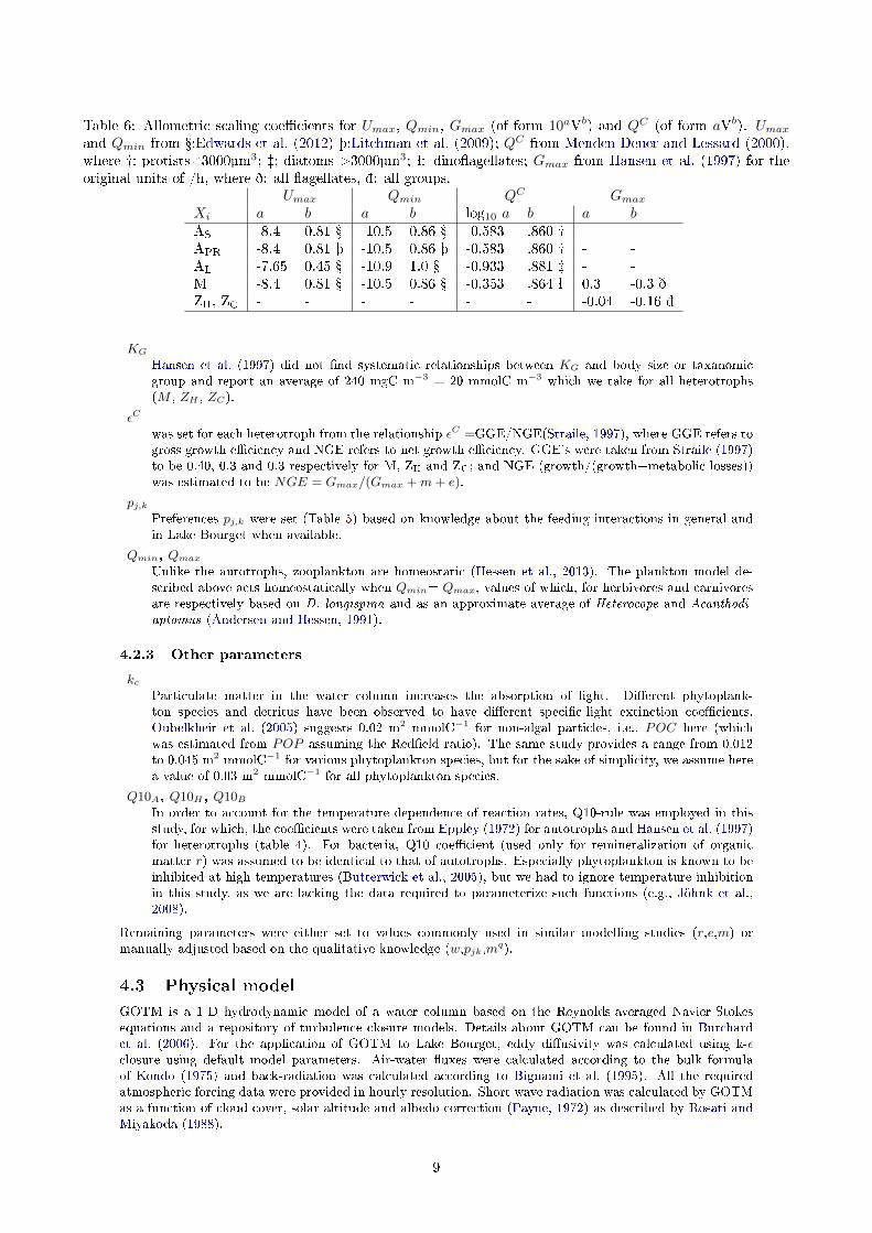
Table 6: Allometric scaling coe�cients for Umax, Qmin, Gmax (of form 10aVb) and QC (of form aVb). Umax

and Qmin from �:Edwards et al. (2012) þ:Litchman et al. (2009); QC from Menden-Deuer and Lessard (2000),where �: protists<3000µm3; �: diatoms >3000µm3; ª: dino�agellates; Gmax from Hansen et al. (1997) for theoriginal units of /h, where ð: all �agellates, �: all groups.

Umax Qmin QC Gmax

Xi a b a b log10 a b a bAS -8.4 0.81 � -10.5 0.86 � -0.583 .860 � - -APR -8.4 0.81 þ -10.5 0.86 þ -0.583 .860 � - -AL -7.65 0.45 � -10.9 1.0 � -0.933 .881 � - -M -8.4 0.81 � -10.5 0.86 � -0.353 .864 ª 0.3 -0.3 ðZH, ZC - - - - - - -0.04 -0.16 �

KG

Hansen et al. (1997) did not �nd systematic relationships between KG and body size or taxanomicgroup and report an average of 240 mgC m−3 = 20 mmolC m−3 which we take for all heterotrophs(M , ZH , ZC).

εC

was set for each heterotroph from the relationship εC =GGE/NGE(Straile, 1997), where GGE refers togross growth e�ciency and NGE refers to net growth e�ciency. GGE's were taken from Straile (1997)to be 0.40, 0.3 and 0.3 respectively for M, ZH and ZC; and NGE (growth/(growth+metabolic losses))was estimated to be NGE = Gmax/(Gmax +m+ e).

pj,kPreferences pj,k were set (Table 5) based on knowledge about the feeding interactions in general andin Lake Bourget when available.

Qmin, QmaxUnlike the autotrophs, zooplankton are homeostatic (Hessen et al., 2013). The plankton model de-scribed above acts homeostatically when Qmin= Qmax, values of which, for herbivores and carnivoresare respectively based on D. longispina and as an approximate average of Heterocope and Acanthodi-aptomus (Andersen and Hessen, 1991).

4.2.3 Other parameters

kcParticulate matter in the water column increases the absorption of light. Di�erent phytoplank-ton species and detritus have been observed to have di�erent speci�c-light extinction coe�cients.Oubelkheir et al. (2005) suggests 0.02 m2 mmolC−1 for non-algal particles, i.e., POC here (whichwas estimated from POP assuming the Red�eld ratio). The same study provides a range from 0.012to 0.045 m2 mmolC−1 for various phytoplankton species, but for the sake of simplicity, we assume herea value of 0.03 m2 mmolC−1 for all phytoplankton species.

Q10A, Q10H , Q10BIn order to account for the temperature dependence of reaction rates, Q10-rule was employed in thisstudy, for which, the coe�cients were taken from Eppley (1972) for autotrophs and Hansen et al. (1997)for heterotrophs (table 4). For bacteria, Q10 coe�cient (used only for remineralization of organicmatter r) was assumed to be identical to that of autotrophs. Especially phytoplankton is known to beinhibited at high temperatures (Butterwick et al., 2005), but we had to ignore temperature inhibitionin this study, as we are lacking the data required to parameterize such functions (e.g., Jöhnk et al.,2008).

Remaining parameters were either set to values commonly used in similar modelling studies (r,e,m) ormanually adjusted based on the qualitative knowledge (w,pjk,mq).

4.3 Physical model

GOTM is a 1-D hydrodynamic model of a water column based on the Reynolds-averaged Navier-Stokesequations and a repository of turbulence closure models. Details about GOTM can be found in Burchardet al. (2006). For the application of GOTM to Lake Bourget, eddy di�usivity was calculated using k-εclosure using default model parameters. Air-water �uxes were calculated according to the bulk formulaof Kondo (1975) and back-radiation was calculated according to Bignami et al. (1995). All the requiredatmospheric forcing data were provided in hourly resolution. Short wave radiation was calculated by GOTMas a function of cloud cover, solar altitude and albedo correction (Payne, 1972) as described by Rosati andMiyakoda (1988).

9

In GOTM, the only source term for heat arises from the attenuation of the shortwave radiation I acrossthe water column, described as the sum of photosynthetically non-active and active radiation:

I(z) = I0ae− zη1 + I0(1− a)e−

zη2−∫ 0z

∑i kc,ici(z

′)dz′ (18)

where I0 is the short wave radiation at the surface, a is the weighting parameter for the di�erentialattenuation of the red and blue-green wavelength components of the light spectrum, η1 and η2 are thecorresponding absorption length scales, and ci (as in eq. 1) and kc,i are, respectively the concentration andthe speci�c extinction coe�cient of item i, constituting the feedback of the coupled biological model to thephysical model. The second term in eq.18 corresponds to IPAR (in eq.5). To account for the backgroundturbidity due to suspended material not explicitly accounted for by the model, Jerlov-IA optical class wasassumed, corresponding to a = 0.62, η1 = 0.6 and η2 = 20 (Paulson and Simpson, 1977).

4.4 Model coupling and operation

The biological model was developed within the Framework of Aquatic Biogeochemical Models (FABMBruggeman and Bolding, 2014). FABM acts as an interface between the biogeochemical model and physicalmodel, GOTM which acts as the host of the biological model, by performing the numerical integration ofthe advection-di�usion-reaction equations (eq.1). According to the on-line coupling scheme employed; statevariables of the biogeochemical model are advected based on the the settling rates (ω in eq.1) speci�ed by thebiogeochemical model and vertical di�usion rates as a function of eddy di�usivity (Kz in eq.1) and verticalgradients (eq.1); ambient water temperature (T ) and (IPAR) estimated by GOTM is provided to the biolog-ical model; and in return, absorption of heat (eq.18) is in�uenced by the concentration of the biological statevariables. Through the GOTM-FABM coupler interface (a Fortran namelist �le), discretization scheme foradvection was chosen as the ULTIMATE QUICKEST algorithm and the source-sink dynamics was chosento be discretized by the 4th order Runge-Kutta scheme. Simulations were ran with an integration time stepof 300 seconds and a vertical resolution of 1 m. Changing the vertical resolution to 0.5 m and time step to100 seconds was observed to make no di�erence.

A number of processes that are required for an accurate simulation of the winter mixing are not resolvedby the coupled physical-biological model system. These include the variation of the mass and energy contentof each vertical layer with depth (i.e., lake hypsography), benthic-pelagic exchange at the lake bottom,various overwintering strategies of plankton, and the pressure sensitivity of the gas vesicles of P. rubescens,which determine their ability to regulate their buoyancy later in the season (which itself is also not resolvedanyway).Therefore, simulations were started each year shortly before the onset of strati�cation, precisely ona date when �eld data that can be used as initial conditions exist. For the initial conditions for temperature,vertically resolved pro�les were used. For the initial phytoplankton and zooplankton concentrations, i.e.,XCi,0, for which only integrated data respectively from top 20 m and 50 m are available, we assumed that the

measured concentrations were homogeneous throughout the water column. For the initial concentration ofdissolved nutrients, i.e., DIP0, no di�erence was observed between using vertical pro�les and homogeneousdistribution (obtained by averaging the vertical pro�le), so we assumed homogeneous distributions, whichfacilitated testing the model sensitivity to phosphorus availability in the system. The concentration of initialparticulate organic phosphorus, POP0 was calculated as POP0 = TP −DIP0 −

∑iX

Pi,0, where TP stands

for measured total phosphorus and XPi,0 = XC

i,0 ∗Qmax,i implying that the plankton were at their maximumquota, as a result of being exposed to high nutrient concentrations throughout the winter. For all thebiological variables, no-�ux boundary condition was assumed both for the surface and bottom of the watercolumn.

4.5 Skill assessment metrics

For evaluating the success of the physical model, we used Taylor & Target diagrams (Jolli� et al., 2009).In Target diagrams, standard deviation normalized model bias (B*), and standard deviation normalizedunbiased (calculated from the anomalies around the means) root mean square deviation (RMSD), multipliedby the sign of the di�erence between the standard deviation of model and observation are mapped onCartesian coordinates. In Taylor diagrams, correlation coe�cients between the observations and simulations,and the standard deviation of the model, normalized to that of the observations (equal at 1) are mapped as,respectively, the angle and radius on polar coordinates.

5 Results

Temporal occurrence and taxonomic composition of each phytoplankton group for the simulated years areshown in Fig. 3. Occurrence of the small algae, AS do not seem to follow a systematic pattern: while in 2006and 2009, this group, represented mainly by small diatoms, was the major contributor of the spring blooms,in 2005, mainly consisting of cyanobacteria, they were responsible for an intense autumn bloom and �nally

10

in 2004 and 2010 this group made up a relatively low and stable background algal biomass throughout theyear. AL were in most years responsible for the spring blooms with a major contribution by diatoms, but in2004, they were abundant also throughout the summer and autumn. Majority of mixotrophs, M , appearedin summer, without any obvious systematic pattern with regard to their taxonomic constituents.

Phytoplankton growth and limitation functions with the parameters speci�ed for each group listed inTable. 3 are shown in Fig. 4, facilitating a comparison between the groups and understanding the successionpatterns shown in Fig. 3. AS is characterized by highest growth rate and nutrient uptake rates, partiallyexplaining its abundance in spring and autumn. AL also has relatively high growth rates, but it hassigni�cantly slower nutrient uptake rates, explaining its absence in summer. APR is characterized by thelowest growth rates, explaining its delayed growth in the season in most years, and lowest light requirementsand greatest high-irradiance intolerance explaining its growth in deeper layers (Jacquet et al., 2014b). Mgrow almost as slow as the APR, and is poor in both light and nutrient acquisition.

Figure 3: Measured contribution of major taxonomic classes to each phytoplankton group throughout thesimulated years.

Figure 4: Limitation functions and their e�ects on autotrophic functions for each plankton group with theparameter values listed in Tables 3-4. fT , fQ, fI and fN stand for temperature limitation (eq. 16), nutrientlimitation of biomass growth (eq. 3), light limitation of photosynthesis (eq. 5) and nutrient limitation of uptake(eq. 8), respectively.

Seasonal and spatial distributions of the state variables estimated by the model are in general reasonable,as exempli�ed for the year 2004 in Fig.5. As the surface waters warm and thermal strati�cation develops at

11

around mid-March, the mixed layer becomes con�ned to the surface layers. This relieves phytoplankton fromlight limitation, leading to blooms of rapid growing AS and AL, and consumption of DIP within the mixedlayer. Phytoplankton growth fuels mixotrophs and herbivorous zooplankton, leading to POP productionand consequently further growth of mixotrophs. Increasing abundances of herbivorous zooplankton andmixotrophs result in a summer-bloom of carnivorous zooplankton, suppressing, in turn, herbivory and hence,preventing the collapse of AS . Autumn is dominated by P. rubescens, which has been growing since mid-summer and at increasingly deeper layers, reaching to about 15-20 meters towards the end of autumn. Theseason ends with strati�cation gradually weakening and mixed-layer extending back to deeper layers.

Figure 5: Spatio-temporal distribution of simulated major variables in 2004.

Comparison of measured and model-estimated concentrations of individual plankton groups, and of watertemperature, dissolved inorganic phosphorus, total phytoplankton (

∑iAi), mixotrophs, total zooplankton

(∑i Zi), and total phosphorus (= DIP + POP +

∑iAi + M +

∑i Zi); all averaged across the top 20

meters of the water column are provided in Fig.6-7. The visual comparisons for the same set of variablesare complemented by Taylor-Target diagrams (Fig. 8). For the case of water temperature, DIP and TP,for which, depth-resolved data are available, Taylor-Target diagrams made with point-wise comparisons for0-80m are given in Fig.9.

12

The match between the measured and simulated water temperatures is outstanding. For DIP in the top20 meters, the spring draw-down, and late-spring replenishment in some years was reproduced, althoughthe latter was underestimated in 2010. The gradual withdrawal of TP throughout the season is also wellreproduced. Slightly higher model estimations at the beginning of the simulations re�ect uncertaintiesregarding the phosphorus content of the cells, which we assumed to be at Qmax, and the value of Qmaxespecially for P. rubescens, which is usually the most abundant species in the system by the end of winter.Skill metrics for both DIP and TP calculated for the upper 20 m are good (Fig.8), characterized by near-zeromodel bias and correlation coe�cients at around 0.8.

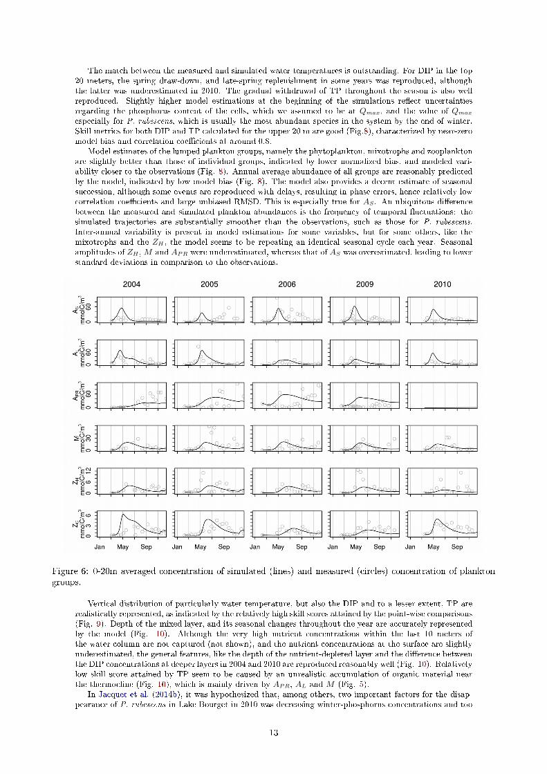
Model estimates of the lumped plankton groups, namely the phytoplankton, mixotrophs and zooplanktonare slightly better than those of individual groups, indicated by lower normalized bias, and modeled vari-ability closer to the observations (Fig. 8). Annual average abundance of all groups are reasonably predictedby the model, indicated by low model bias (Fig. 8). The model also provides a decent estimate of seasonalsuccession, although some events are reproduced with delays, resulting in phase errors, hence relatively lowcorrelation coe�cients and large unbiased RMSD. This is especially true for AS . An ubiquitous di�erencebetween the measured and simulated plankton abundances is the frequency of temporal �uctuations: thesimulated trajectories are substantially smoother than the observations, such as those for P. rubescens.Inter-annual variability is present in model estimations for some variables, but for some others, like themixotrophs and the ZH , the model seems to be repeating an identical seasonal cycle each year. Seasonalamplitudes of ZH ,M and APR were underestimated, whereas that of AS was overestimated, leading to lowerstandard deviations in comparison to the observations.

Figure 6: 0-20m averaged concentration of simulated (lines) and measured (circles) concentration of planktongroups.

Vertical distribution of particularly water temperature, but also the DIP and to a lesser extent, TP arerealistically represented, as indicated by the relatively high skill scores attained by the point-wise comparisons(Fig. 9). Depth of the mixed layer, and its seasonal changes throughout the year are accurately representedby the model (Fig. 10). Although the very high nutrient concentrations within the last 10 meters ofthe water column are not captured (not shown), and the nutrient concentrations at the surface are slightlyunderestimated, the general features, like the depth of the nutrient-depleted layer and the di�erence betweenthe DIP concentrations at deeper layers in 2004 and 2010 are reproduced reasonably well (Fig. 10). Relativelylow skill score attained by TP seem to be caused by an unrealistic accumulation of organic material nearthe thermocline (Fig. 10), which is mainly driven by APR, AL and M (Fig. 5).

In Jacquet et al. (2014b), it was hypothesized that, among others, two important factors for the disap-pearance of P. rubescens in Lake Bourget in 2010 was decreasing winter-phosphorus concentrations and too

13

Figure 7: 0-20m averaged concentration of simulated (lines) and measured (circles) concentration of biologicalvariables.

Figure 8: Target-Taylor diagrams for 0-20 m average concentration of (top) individual plankton groups and(bottom) dissolved phosphorus and total phosphorus, total phytoplankton, total mixotrophs and total zooplank-ton carbon biomass.

small winter inoculum. Despite the fact that no P. rubescens was detected in the phytoplankton assemblagesthroughout the year 2010, the model was initiated with a winter inoculum of 10−2 mmolC/m3, which is close

14

Figure 9: Target-Taylor diagrams for temperature, dissolved phosphorus and total phosphorus within the upper80 m, depth-resolution retained, unlike in Fig.8

to the minimum observed concentration in 2004. Starting from this small inoculum, P. rubescens biomassdid not grow substantially (Fig. 6)). In order to gain some insight into the reasons that eliminated P.rubescens from the system, a scenario analysis was performed, where the initial, winter concentrations ofP. rubescens and DIP were replaced with the values observed in 2004 (Fig. 11). Higher initial DIP (0.91instead of 0.46 mmol/m3) resulted in slightly higher P. rubescens concentrations, although the di�erencewas not appreciable. On the other hand, higher winter inoculum (0.62 instead of 0.01 mmol/m3) resultedin larger than 10 mmol/m3 of P. rubescens during autumn. Setting both the DIP and APR concentrationsto 2004 values resulted in dynamics very similar to those obtained in 2004, suggesting that other di�erencesbetween these two years, e.g., with respect to the meteorological conditions and initial concentration of otherplankton groups, were not critical in determining P. rubescens dynamics.

6 Discussion

In this study, we described a novel biogeochemical model coupled to a 1-D hydrodynamical model, and itsapplication to Lake Bourget. We demonstrate that the model is able to provide a reasonable representationof the seasonal phosphorus cycle and to some extent, the succession of the plankton groups in this ecosystem.Our scenario analysis suggests that the winter concentration of P. rubescens has a determining role for itsdynamics in the following growth season.

The model is implemented as three FABM (Bruggeman and Bolding, 2014) modules, which can becoupled at run-time (i.e., without the need for changing and re-compiling the model code): a nutrientmodule, a detritus module, and a plankton module that can be placed anywhere along the autotrophy-heterotrophy continuum (Flynn et al., 2012) with the 'autotrophy fraction' parameter ζ, enabled by ageneralized formal description of autotrophic and heterotrophic processes (Section 4.1). In the presentimplementation, the plankton module is coupled six times to describe interactions of three purely autotrophic,two purely heterotrophic and a mixotrophic plankton groups. Realistic representation of spatio-temporaldistribution of inorganic and particulate phosphorus, as well as the plankton groups constitute a proof ofthe concept. These generic modules thus enable description of various food web con�gurations in run-timeand therefore can facilitate site-speci�c con�gurations in future studies.

Incorporation of mixotrophy is another novel aspect of the current study, given that mixotrophy has been,with exceptions (e.g., Ward and Follows, 2016), neglected in ecosystem scale model applications. Here, thedescription of mixotrophy is quite simplistic, relying on the assumption that there exists a linear trade-o�between autotrophic and heterotrophic abilities (Crane and Grover, 2010), and the assumption that theparameters of heterotrophic and autotrophic traits re�ect the conditions that enforced pure heterotrophy orautotrophy in the meta-analysis data that formed the basis for parameterization in this study. It should befurther noted that, in reality, a major carbon and nutrient source for mixotrophs is often bacteria (Mitraet al., 2014), which is not explicitly modelled in this study, but is implicitly represented by the POM pool, Pcontent of which is known, but C content is assumed to be proportional to P by the Red�eld ratio. Furtherresolution of the microbial loop and the organic matter pools in Lake Bourget would be out of the scopeof the current study, but constitutes a potential future goal, as with ongoing oligotrophication, relativeimportance of mixotrophs in the system can be anticipated to increase (Kamjunke et al., 2007; Mitra et al.,2014).

In this study, mixotrophs and herbivorous and carnivorous zooplankton were assigned as individualfunctional groups based on their position in the food web. P. rubescens was assigned as a separate algal groupbecause of its distinctive eco-physiology characterized by low-light tolerance (Walsby and Schanz, 2002), slowgrowth (Bright and Walsby, 2000), and grazing defense (Kurmayer and Jüttner, 1999) as well as the factthat it represented about half of the phytoplankton assemblage in some years (Fig. 1,3). Previous modelling

15

Figure 10: Simulated (lines) and measured (circles) Temperature, DIP and TP pro�les from 2004 and 2010within the upper 80 m. Only the �rst measurements in each month are shown. Pro�les from identical monthsin di�erent years are aligned.

16

DIP0=0.46, PR0=0.01

DIP0=0.91, PR0=0.01

DIP0=0.46, PR0=0.62

DIP0=0.91, PR0=0.62

Figure 11: Surface (0-20 m) average water column average state variables with initial DIP concentration ofDIP0 = 0.46 mmolP m−3 as in 2010 (solid lines), DIP0 = 0.91 mmolP m−3 as in 2004 (dashed lines), incombination with initial P. rubescens concentration of PR0 = 0.01 mmolC m−3 as (was assumed) in 2010(no marker) and PR0 = 0.62 mmolC m−3 as in 2004 (triangles). Initial conditions for all other variables andmeteorological forcing was as in 2010.

studies focusing on similarly P. rubescens-infested lakes unequivocally assigned P. rubescens an own group(Omlin et al., 2001; Copetti et al., 2006; Mieleitner and Reichert, 2008; Carraro et al., 2012). Remainingphytoplankton were separated by size, forming 'small' and 'large' algal groups, given the importance of sizein determining light and light utilization traits, among others (Finkel et al., 2010). There exist modellingstudies where taxonomic classes were parameterized directly as functional groups (e.g., Jöhnk et al., 2008;Carraro et al., 2012), but categorization based on size, thereby combining di�erent taxonomic classes withina given functional group like in this study is not uncommon (e.g., Mieleitner and Reichert, 2008; Gal et al.,2009; Rinke et al., 2010).

Parameterization of the plankton groups was largely based on allometric relationships and taxonomicproperties, inspired by recent meta-analyses (Litchman et al., 2009; Schwaderer et al., 2011; Edwards et al.,

17

2012). This approach was to some extent necessary, due to the lack of information on physiological parame-ters of the speci�c plankton species or groups observed in Lake Bourget. On the other hand, we believe thatthis approach should produce a more consistent and transferable (i.e., applicable to other systems) parameterset than that could be obtained by a pure calibration exercise, which is problematic due to poor parameteridenti�ability of plankton functional group models (Anderson, 2005; Mieleitner and Reichert, 2008). In thisstudy, parameter tuning was restricted to parameters like zooplankton preferences, sinking rates (of ALand detritus) and remineralization rates. Setting zooplankton feeding preferences is a common problem inecosystem models, as model results are sensitive to di�erent parameterizations (Gentleman et al., 2003), andas the experimental data so far are based on speci�c prey-predator pairs that are hardly generalizable. Forthe parameterization of sinking and remineralization rates, we acknowledge potential biases in the form ofan underestimation of sinking rates and an overestimation of remineralization rates to compensate the lackof river nutrient �uxes.

Based on the classical variable internal stores model schemes, the storage capacity, Qmax/Qmin has beenshown to have a critical importance in the presence of temporal (Grover, 1991) and/or spatial (Kerimogluet al., 2012) heterogeneity. Di�erent allometric scalings observed in Qmax and Qmin for nitrogen, contrastingwith similar coe�cients in those for phosphorus have been suggested to explain marine diatoms being largerthan freshwater diatoms (Litchman et al., 2009). On the other hand, it is questionable whether Qmaxshould be considered as a �xed physiological parameter, as the observed maximum nutrient contents inphytoplankton cells might as well be re�ecting the acclimative down-regulation of the uptake rate, whichdepends on the speci�c settings, like limitation by other nutrients, supply rates and light limitation, asshown by optimality based model schemes (Pahlow et al., 2013; Wirtz and Kerimoglu, 2016). This might bethe reason for lack of robust patterns in distributions of Qmax across cell size or taxa, hence, its exclusionfrom analyses aiming to identify allometric and taxonomic variations in physiological traits (e.g., Litchmanet al., 2007; Edwards et al., 2012). In this study, acknowledging the poor understanding of the issue, weassumed a �xed proportionality between Qmax and Qmin, in order to avoid introducing a potentially strongbut unjusti�ed trait that can e�ect the competitive outcomes.

Overall, the model performance is good, given the limitations of the idealized 1-D approach. Modelestimates for water temperature are almost excellent (Fig. 7-10). Average surface concentrations of DIP andTP can considered to be very good (r>0.85, Fig.8). The measured DIP concentrations during summer tendto be somewhat higher than the simulations, which might be, to some extent, due to the river �uxes that notrepresented by the model, however, considering the long water residence time of the lake (about 10 years)there is probably some other mechanism involved. Vertical pro�les of DIP, and to a lesser extent, TP withinthe upper 80 m are quite realistically reproduced by the model. Annual average concentration of planktongroups are well reproduced, indicated by low bias, but the seasonal dynamics is poorly represented, resultingin phase errors, and low correlation coe�cients (Fig. 6). Interannual variability of the data is also morepronounced than that of the simulations. Especially P. rubescens follows contrasting patterns in di�erentyears: in the form of smooth patterns in 2004 and 2009, and very rapid changes in the years 2005 and2006, which are likely to be related with some vertical or lateral transport mechanism like those inducedby internal waves or upwelling events that occur frequently in Lake Bourget (Cuypers et al., 2011), giventheir low growth rates (Bright and Walsby, 2000) and limited losses imposed by zooplankton (Kurmayer andJüttner, 1999). On the other hand, their growth at 10-20 m depth (Fig. 5) notably coincides well with theobservations in Lake Bourget (Jacquet et al., 2005, 2014b; Le Vu et al., 2011). In reality, this phenomenais usually attributed to buoyancy regulation (Walsby et al., 2004), whereas in this study, no active mobilitymechanism has been considered and their sub-surface growth largely re�ects the parameterized low-lighttolerance and high-light inhibition of the species (Walsby and Schanz, 2002). The depth-dependent mortalitywe assumed for P. rubescens (eq.14) does not play a signi�cant role in the occurrence of such thin layers,whereas it certainly pulls the depth of maximum concentration a few meters upwards. Our preliminary work(not shown) suggest that the thin-layers can be represented by specifying an optimum growth temperature orirradiance, however, using a process-based buoyancy regulation model (e.g., Kromkamp and Walsby, 1990)would be more useful for gaining a better understanding of the relevance of the formation of thin layers.Finally, high frequency �uctuations in other variables are not captured, which might be related with extremeriver discharge events (Vinçon-Leite et al., 1995) in the system. A 3-D modelling study revealed that in arelatively smaller (surface area: 5 km2) Lake Pusiano, a major �ood event caused a signi�cant variation inthe horizontal distribution of P. rubescens (Carraro et al., 2012). Given that the two major tributaries ofLake Bourget are in the South (Bryhn et al., 2010), and the out�ows are in the North, such can be expectedin Lake Bourget as well to some extent, but the e�ects are presumably smaller due to the much smallerquantity of �uxes in relation to the water volume in Lake Bourget in comparison to Lake Pusiano, whichhas a water residence time of about 1 year (Carraro et al., 2012), i.e., one tenth that of Lake Bourget.

Occurrence of P. rubescens is usually attributed to the nutrient availability, when long-term dynamics(Dokulil and Teubner, 2012; Posch et al., 2012) and lakes at di�erent trophic states are considered (Salmasoet al., 2012; Anneville et al., 2015). Within our study period, winter DIP fell from 0.9 to 0.46 mmolP/m3

(corresponding to 27.9 to 14.3 mgP/m3) between 2004 and 2010 (Fig. 1), which does not encompassa large range relative to the above examples. Indeed, our scenario analysis where we used the winter

18

DIP concentration of 2004 for simulating 2010 did not result in a signi�cant di�erence from the referencesimulation of 2010 (Fig. 11). In contrary, when the winter concentration of P. rubescens in 2004 wasused for simulating 2010, a large P. rubescens bloom was formed, unlike the reference simulation of 2010(Fig. 11). These results suggest that the initial abundances by the end of the winter are highly importantfor the dynamics of P. rubescens within the growth season, which is in line with the �ndings of Jacquetet al. (2014b), who showed a signi�cant relationship between the winter-spring, spring-summer and summer-autumn biomasses. Qualitatively the same results were obtained when the scenario analysis was repeatedwith an altered model parameterization (not shown), where, P. rubescens was described as a species withslightly stronger resource competition traits (50% lower KU and 25% higher µ∞, given the uncertainties ofthe allometric scaling of these parameters), and slighty weaker defense against predation (mixotrophs feedingon them with pM,k=0.5,0.4 and 0.1 for k=POM, AS and APR, given the lacking evidence for the feedinginteractions between P. rubescens and mixotrophic species in Lake Bourget).

The sensitivity of growing season P. rubescens abundance to the initial population size after winter doesnot simply result from a delayed geometric growth: when the scenario analysis is repeated with a structurallydi�erent model where P. rubescens is the only autotroph, i.e., not having any competitors, even the scenariowith low initial inoculum and phosphorus concentrations results in a substantial bloom with concentrationsreaching up to 50 mmolC m−3 (Appendix B), which is close to the concentrations observed in the years withintense P. rubescens occurrences. These �ndings therefore suggest that the disappearance of P. rubescensfrom Lake Bourget was actually due to competitive exclusion, facilitated by the phenomena called thepriority e�ect (Hodge et al., 1996), in which, the species with higher initial concentrations outcompetetheir competitors with lower initial concentrations by making the abiotic environment inhabitable by theothers. The priority e�ect has been previously reported from �eld measurements (Tapolczai et al., 2014) andmesocosm experiments (Sommer and Lewandowska, 2011). Vertical distributions obtained under di�erentscenarios (not shown) suggest that the priority e�ect is manifested as a bistability of both phytoplanktoncomposition and vertical distribution of phytoplankton biomass (as in Ryabov et al., 2010). When P.rubescens start the season from relatively higher concentrations, they end up being the dominant speciesstarting from summer by forming a dense layer at the metalimnion and thereby prevent the growth of mainlythe small species through intensifying the nutrient limitation in the upper layers. To the contrary, whenthey start from low concentrations, small phytoplankton persist in the surface layers throughout the summer,making it thereby di�cult for P. rubescens to grow through intensifying light limitation. The self-stabilizingnature of these two alternative states may partially explain the inter-annual variability of the P. rubescensabundances commonly observed in various deep lakes (Vinçon-Leite et al., 2002; Salmaso, 2010; Jacquetet al., 2014b; Anneville et al., 2015).

It should be noted that, although the additional P. rubescens growth caused by higher initial phosphoruswas relatively small, the higher P. rubescens concentration by the beginning of winter might be of substantialimportance for the dynamics that follow later in the next season, as scenarios with higher initial P. rubescensconcentrations suggest (Fig. 11). Moreover, the range of phosphorus concentrations in this scenario analysisis relatively small relative to the historical observations in Lake Bourget itself and in other lakes, so it doesnot imply that phosphorus availability is unimportant for the occurrence of this P. rubescens. In contrary,we believe that the long-term decrease of phosphorus in Lake Bourget was a prerequisite for the �naldisappearance of P. rubescens as suggested by (Jacquet et al., 2014b). A model-aided test of this hypothesiscan be achieved with a model validated for contrasting conditions with respect to the trophic state and theavailability of P. rubescens that are observed either in a single lake across a long-term transition, or multiplelakes of di�erent trophic status.

In Lake Bourget (Vinçon-Leite et al., 2002; Jacquet et al., 2014b; Anneville et al., 2015), as well as inother deep lakes like Lake Zurich (Walsby et al., 1998; Posch et al., 2012), Lake Garda (Salmaso, 2010)and Mondsee (Dokulil and Teubner, 2012), the abundance of P. rubescens by the end of winter is largelydetermined by meteorological conditions during winter. In such deep, warm monomictic lakes, cooling inmild winters may end up being insu�cient to cause a full overturn, leading to a reduced dilution of the P.rubescens concentrations, as well more P. rubescens cells survive the winter (Walsby et al., 1998). Beyondthe fact that phosphorus reached low concentrations in Lake Bourget, it seems like the coincidence of sucha cold winter with a weak autumn population, might be the explanation for the complete elimination of theP. rubescens in 2010. Indeed, in 2010, both the autumn and winter air temperatures were among the coldestin the region (Anneville et al., 2015), and P. rubescens had a relatively low autumn concentration (Jacquetet al., 2014b, and this study, Fig 6). In this context, it is worth noting that the warming trend observed inLake Bourget (Vinçon-Leite et al., 2014) can be expected to further continue given the anticipated warmingof especially the winters in the alpine region (Beniston, 2006), possibly promoting the re-establishment ofP. rubescens in Lake Bourget, given the evidence that warming promoted P. rubescens in Lake Zurich(Anneville et al., 2004) and Lake Geneva (Gallina et al., 2017).

In Lake Bourget, mixing does not reach the lake bottom during warm winters, such as in 2007 and 2008,which leads to signi�cantly lower phosphorus concentrations and high P. rubescens abundances later in theseason season (Jacquet et al., 2014b). Therefore an extended model based analysis of plankton successionencompassing the winter dynamics would be highly relevant. Although the model presented in this study

19

can serve as a starting point, several other processes need to be taken into account, including the lakehypsography, benthic-pelagic exchange, overwintering strategies of plankton, and the buoyancy regulationof P. rubescens, as well its inhibition through collapsing of gas vesicles under high pressure. Other rarebehavior of P. rubescens worth considering in future modelling studies include colony formation behaviorand its e�ect on predation by zooplankton. In this study, we assumed a non-zero but low preference of P.rubescens by the herbivorous zooplankton, but the evidence suggests that the grazing rate depends on thecolony size (Oberhaus et al., 2007), and there is a signi�cant relationship between the nutrient status andcolony size (Jacquet et al., 2014b), suggesting that this preference should not be constant in time and space.Acknowledgements

This study is a contribution to the PhyCl project and to the observatory of alpine lakes (OLA). Data weremade available by SOERE OLA-IS, INRA Thonon les Bains, CISALB and ecoinformatics ORE-INRA team.Authors are grateful to all the technicians, engineers and researchers who have contributed to the monitoringof Lake Bourget. We thank two anonymous referees for their comments. Funding for OK was provided bythe University of Savoie Mont Blanc (AAP 2012). OK was additionally supported by the German ResearchFoundation (DFG) through the priority program 1704 `DynaTrait'.

References

Andersen, T., Hessen, D.O., 1991. Carbon, nitrogen, and phosphorus content of freshwater zooplankton.Limonology And Oceanography 36, 807�814.

Anderson, T.R., 2005. Plankton functional type modelling: running before we can walk? Journal of PlanktonResearch 27, 1073�1081.

Anneville, O., Domaizon, I., Kerimoglu, O., Rimet, F., Jacquet, S., 2015. Blue-Green Algae in a �GreenhouseCentury�? New Insights from Field Data on Climate Change Impacts on Cyanobacteria Abundance.Ecosystems 18, 441�458.

Anneville, O., Souissi, S., Gammeter, S., Straile, D., 2004. Seasonal and inter-annual scales of variabilityin phytoplankton assemblages: comparison of phytoplankton dynamics in three peri-alpine lakes over aperiod of 28 years. Freshwater Biology 49, 98�115.

Armstrong, R., 1994. Grazing limitation and nutrient limitation in marine ecosystems: Steady state solutionsof an ecosystem model with multiple food chains. Limonology And Oceanography 39, 597�608.

Beniston, M., 2006. Mountain weather and climate: A general overview and a focus on climatic change inthe Alps. Hydrobiologia 562, 3�16.

Berge, T., Chakraborty, S., Hansen, P.J., Andersen, K.H., 2017. Modeling succession of key resource-harvesting traits of mixotrophic plankton. The ISME journal 11, 212�223.

Bignami, F., Marullo, S., Santoleri, R., Schiano, M.E., 1995. Longwave radiation budget in the MediterraneanSea. Journal of Geophysical Research 100, 2501.

Briand, J.F., Jacquet, S., Flinois, C., Avois-Jacquet, C., Maisonnette, C., Leberre, B., Humbert, J.F.,2005. Variations in the microcystin production of Planktothrix rubescens (cyanobacteria) assessed froma four-year survey of Lac du Bourget (France) and from laboratory experiments. Microbial Ecology 50,418�428.

Bright, D., Walsby, A., 2000. The daily integral of growth by Planktothrix rubescens calculated from growthrate in culture and irradiance in Lake Zürich. New Phytologist 146, 301�316.

Bruggeman, J., Bolding, K., 2014. A general framework for aquatic biogeochemical models. EnvironmentalModelling & Software 61, 249�265.

Bryhn, A., Girel, C., Paolini, G., Jacquet, S., 2010. Predicting future e�ects from nutrient abatementand climate change on phosphorus concentrations in Lake Bourget, France. Ecological Modelling 221,1440�1450.

Burchard, H., Bolding, K., Kühn, W., Meister, A., Neumann, T., Umlauf, L., 2006. Description of a �exibleand extendable physical-biogeochemical model system for the water column. Journal of Marine Systems61, 180�211.

Butterwick, C., Heaney, S.I., Talling, J.F., 2005. Diversity in the in�uence of temperature on the growthrates of freshwater algae, and its ecological relevance. Freshwater Biology 50, 291�300.

20

Carraro, E., Guyennon, N., Hamilton, D., Valsecchi, L., Manfredi, E.C., Viviano, G., Salerno, F., Tartari,G., Copetti, D., 2012. Coupling high-resolution measurements to a three-dimensional lake model to assessthe spatial and temporal dynamics of the cyanobacterium Planktothrix rubescens in a medium-sized lake.Hydrobiologia 698, 77�95.

Chen, B., Liu, H., 2010. Relationships between phytoplankton growth and cell size in surface oceans:Interactive e�ects of temperature, nutrients, and grazing. Limnology and Oceanography 55, 965�972.

Copetti, D., Tartari, G., Morabito, G., Oggioni, A., Legnani, E., 2006. A biogeochemical model of LakePusiano (North Italy) and its use in the predictability of phytoplankton blooms: �rst preliminary results.J. Limnol. 65, 59�64.

Crane, K., Grover, J., 2010. Coexistence of mixotrophs, autotrophs, and heterotrophs in planktonic microbialcommunities. Journal of Theoretical Biology 262, 517�527.

Cuypers, Y., Vinçon-Leite, B., Groleau, A., Tassin, B., Humbert, J.F., 2011. Impact of internal waves onthe spatial distribution of Planktothrix rubescens (cyanobacteria) in an alpine lake. The ISME journal 5,580�589.

Dokulil, M.T., Teubner, K., 2012. Deep living Planktothrix rubescens modulated by environmental con-straints and climate forcing. Hydrobiologia 698, 29�46.

Droop, M., 1968. Vitamin B12 and marine ecology. IV. The kinetics of uptake, growth and inhibition inMonochrysis lutheri. Journal of the Marine Biological Association of the United Kingdom 48, 689�733.

Druart, J.C., Rimet, F., 2008. Protocoles d'analyse du phytoplancton de l'INRA: prélèvement, dénombre-ment et biovolumes. Technical Report. INRA. Thonon les Bains.

Dumont, H.J., de Velde, I., Dumont, S., 1975. The dry weight estimate of biomass in a selection of Cladocera,Copepoda and Rotifera from the plankton, periphyton and benthos of continental waters. Oecologia 19,75�97.

Edwards, K.F., Thomas, M.K., Klausmeier, C.A., Litchman, E., 2012. Allometric scaling and taxonomicvariation in nutrient utilization traits and maximum growth rate of phytoplankton. Limnol. Oceanogr 57,554�566.

Eppley, R., 1972. Temperature and phytoplankton growth in the sea. Fishery Bulletin 70, 1063�1085.

Ernst, B., Hoeger, S.J., Brien, E.O., Dietrich, D.R., 2009. Abundance and toxicity of Planktothrix rubescensin the pre-alpine Lake Ammersee, Germany. Harmful Algae 8, 329�342.

Fasham, M., Ducklow, H., Mckelvie, S., 1990. A nitrogen-based model of plankton dynamics in the oceanicmixed layer. Journal of Marine Research` 48, 591�639.

Finkel, Z., Beardall, J., Flynn, K., Quigg, A., Rees, T., Raven, J., Raven, J.A., 2010. Phytoplankton in achanging world: cell size and elemental stoichiometry. Journal of plankton research 32, 119�137.

Flynn, K., Stoecker, D., Mitra, A., Raven, J., Glibert, P., Hansen, P.J., Graneli, E., Burkholder, J.M., 2012.Misuse of the phytoplankton-zooplankton dichotomy: the need to assign organisms as mixotrophs withinplankton functional types. Journal of Plankton Research 35, 3�11.

Flynn, K.J., Mitra, A., 2009. Building the �perfect beast�: modelling mixotrophic plankton. Journal ofPlankton Research 31, 965�992.

Gal, G., Hipsey, M., Parparov, A., Wagner, U., Makler, V., Zohary, T., Zohary, T., 2009. Implementationof ecological modeling as an e�ective management and investigation tool: Lake Kinneret as a case study.Ecological Modelling 220, 1697�1718.

Gallina, N., Beniston, M., Jacquet, S., 2017. Estimating future cyanobacterial occurrence and importancein lakes: a case study with Planktothrix rubescens in Lake Geneva. Aquatic Sciences 79, 249�263.

Gentleman, W., Leising, A., Frost, B., Strom, S., Murray, J., 2003. Functional responses for zooplanktonfeeding on multiple resources: a review of assumptions and biological dynamics. Deep-Sea Research II 50,2847�2875.

Grover, J., 1991. Resource competition in a variable environment: phytoplankton growing according to thevariable-internal-stores model. The American Naturalist 138, 811�835.

Grover, J., 2002. Stoichiometry, Herbivory and Competition for Nutrients: Simple Models based on Plank-tonic Ecosystems. J. Theoret. Biol. 214, 599�618.

21

Halstvedt, C., Rohrlack, T., Andersen, T., Skulberg, O., Edvardsen, B., 2007. Seasonal dynamics and depthdistribution of Planktothrix spp. in Lake Steinsfjorden (Norway) related to environmental factors. Journalof Plankton Research 29, 471�482.

Hansen, P., Bjørnsen, P., Hansen, B., 1997. Zooplankton grazing and growth: Scaling within the 2-2,000-µmbody size range. Limnology and Oceanography 42, 687�704.

Hessen, D.O., Elser, J.J., Sterner, R.W., Urabe, J., 2013. Ecological stoichiometry: An elementary approachusing basic principles. Limnology and Oceanography 58, 2219�2236.

Hodge, S., Arthur, W., Mitchell, P., 1996. E�ects of Temporal Priority on Interspeci�c Interactions andCommunity Development. Oikos 76, 350�358.

Hood, R.R., Laws, E.A., Armstrong, R.A., Bates, N.R., Brown, C.W., Carlson, C.A., Chai, F., Doney, S.C.,Falkowski, P.G., Feely, R.A., Friedrichs, M.A.M., Landry, M.R., Moore, J.K., Nelson, D.M., Richardson,T.L., Salihoglu, B., Schartau, M., Toole, D.A., Wiggert, J.D., 2006. Pelagic functional group modeling:Progress, challenges and prospects. Deep Sea Research Part II: Topical Studies in Oceanography 53,459�512.

Jacquet, S., Briand, J.F., Christophe, L., Avois-Jacquet, C., Oberhaus, L., Tassin, B., Vinçon-Leite, B.,Paolini, G., Druart, J.C., Anneville, O., Humbert, J.F., 2005. The proliferation of the toxic cyanobacteriumPlanktothrix rubescens following restoration of the largest natural French lake (Lac du Bourget). HarmfulAlgae 4, 651�672.

Jacquet, S., Domaizon, I., Anneville, O., 2014a. The need for ecological monitoring of freshwaters in achanging world: A case study of Lakes Annecy, Bourget, and Geneva. Environmental Monitoring andAssessment 186, 3455�3476.

Jacquet, S., Kerimoglu, O., Rimet, F., Paolini, G., Anneville, O., 2014b. Cyanobacterial bloom termination:the disappearance of Planktothrix rubescens from Lake Bourget (France) after restoration. FreshwaterBiology 59, 2472�2487.

Jöhnk, K., Huisman, J., Sharples, J., Sommeijer, B., Visser, P., Stroom, J., 2008. Summer heatwavespromote blooms of harmful cyanobacteria. Global Change Biology 14, 495�512.

Jolli�, J., Kindle, J., Shulman, I., Penta, B., Friedrichs, M., Helber, R., Arnone, R., 2009. Summary diagramsfor coupled hydrodynamic-ecosystem model skill assessment. Journal of Marine Systems 76, 64�82.

Kamjunke, N., Henrichs, T., Gaedke, U., 2007. Phosphorus gain by bacterivory promotes the mixotrophic�agellate Dinobryon spp. during re-oligotrophication. Journal of Plankton Research 29, 39�46.

Kerimoglu, O., Straile, D., Peeters, F., 2012. Role of phytoplankton cell size on the competition for nutrientsand light in incompletely mixed systems. Journal of Theoretical Biology 300, 330�343.

Kerimoglu, O., Straile, D., Peeters, F., 2013. Seasonal, inter-annual and long term variation in top-downversus bottom-up regulation of primary production. Oikos 122, 223�234.

Kiørboe, T., 2011. How zooplankton feed: mechanisms, traits and trade-o�s. Biological Reviews of theCambridge Philosophical Society 86, 311�339.

Kondo, J., 1975. Air-sea bulk transfer coe�cients in diabatic conditions. Boundary Layer Meteorology 9,91�112.

Konopka, A., 1982. Buoyancy regulation and vertical migration by Oscillatoria Rubescens in Crooked Lake,Indiana. British Phycological Journal , 427�442.

Kromkamp, J., Walsby, A.E., 1990. A computer model of buoyancy and vertical migration in cyanobacteria.Journal of Plankton Research 12, 161�183.

Kurmayer, R., Jüttner, F., 1999. Strategies for the co-existence of zooplankton with the toxic cyanobacteriumPlanktothrix rubescens in Lake Zürich. Journal of Plankton Research 21, 659�683.

Le Vu, B., Vinçon-Leite, B., Lemaire, B., Bensoussan, N., Calzas, M., Drezen, C., Al., E., 2011. High-frequency monitoring of phytoplankton dynamics within the European water framework directive: appli-cation to metalimnetic cyanobacteria. Biogeochemistry 106, 229�242.

Litchman, E., Klausmeier, C.A., Scho�eld, O.M., Falkowski, P.G., 2007. The role of functional traits andtrade-o�s in structuring phytoplankton communities: scaling from cellular to ecosystem level. EcologyLetters 10, 1170�1181.

22

Litchman, E., Klausmeier, C.A., Yoshiyama, K., 2009. Contrasting size evolution in marine and freshwaterdiatoms. Proceedings of the National Academy of Sciences 106, 2665�2670.

Litchman, E., Pinto, P.D.T., Klausmeier, C.A., Thomas, M.K., Yoshiyama, K., 2010. Linking traits tospecies diversity and community structure in phytoplankton. Hydrolobiologia 653, 15�28.

Menden-Deuer, S., Lessard, E., 2000. Carbon to volume relationships for dino�agellates , diatoms , andother protist plankton. Limnology and Oceanography 45, 569�579.

Mieleitner, J., Reichert, P., 2008. Modelling functional groups of phytoplankton in three lakes of di�erenttrophic state. Ecological Modelling 211, 279�291.

Mitra, A., Flynn, K.J., Burkholder, J.M., Berge, T., Calbet, A., Raven, J.a., Granéli, E., Glibert, P.M.,Hansen, P.J., Stoecker, D.K., Thingstad, F., Tillmann, U., Våge, S., Wilken, S., Zubkov, M.V., 2014. Therole of mixotrophic protists in the biological carbon pump. Biogeosciences 11, 995�1005.

Morel, F., 1987. Kinetics of nutrient uptake and growth in phytoplankton. Journal of Phycology 23, 137�150.

Naselli-Flores, L., Barone, R., Chorus, I., Kurmayer, R., 2007. Toxic Cyanobacterial Blooms in ReservoirsUnder a Semiarid Mediterranean Climate: The Magni�cation of a Problem. Environmental Toxicology22, 399�404.

Oberhaus, L., Gelinas, M., Pinel-Alloul, B., Ghadouani, A., Humbert, J.F., 2007. Grazing of two toxicPlanktothrix species by Daphnia pulicaria: potential for bloom control and transfer of microcystins.Journal of Plankton Research 29, 827�838.

Omlin, M., Reichert, P., Forster, R., 2001. Biogeochemical model of Lake Zürich: model equations andresults. Ecological Modelling 141, 77�103.

Oubelkheir, K., Sciandra, A., Babin, M., 2005. Bio-optical and biogeochemical properties of di�erent trophicregimes in oceanic waters. Limnology and Oceanography 50, 1795�1809.

Padisák, J., Hajnal, É., Krienitz, L., Lakner, J., Üveges, V., 2010. Rarity, ecological memory, rate of �oralchange in phytoplankton�and the mystery of the Red Cock. Hydrobiologia 653, 45�64.

Pahlow, M., Dietze, H., Oschlies, A., 2013. Optimality-based model of phytoplankton growth and diazotro-phy. Marine Ecology Progress Series 489, 1�16.

Paulson, C., Simpson, J., 1977. Irradience measurements in the upper ocean. Journal of Physical Oceanog-raphy 7, 952�956.

Payne, R.E., 1972. Albedo of the Sea Surface. Journal of the Atmospheric Sciences 29, 959�970.

Posch, T., Salcher, M.M., Pernthaler, J., 2012. Harmful �lamentous cyanobacteria favoured by reducedwater turnover with lake warming. Nature Climate Change 2, 809�813.

Rinke, K., Yeates, P., Rothhaupt, K.O., 2010. A simulation study of the feedback of phytoplankton onthermal structure via light extinction. Freshwater Biology 55, 1674�1693.

Robson, B.J., 2014. When do aquatic systems models provide useful predictions, what is changing, and whatis next? Environmental Modelling and Software 61, 287�296.

Rosati, A., Miyakoda, K., 1988. A general circulation model for upper ocean simulation. Journal of PhysicalOceanography 18, 1601�1626.

Ryabov, A., Rudolf, L., Blasius, B., 2010. Vertical distribution and composition of phytoplankton under thein�uence of an upper mixed layer. Journal of Theoretical Biology 263, 120�133.

Salmaso, N., 2010. Long-term phytoplankton community changes in a deep subalpine lake: responses tonutrient availability and climatic �uctuations. Freshwater Biology 55, 825�846.

Salmaso, N., Buzzi, F., Garibaldi, L., Morabito, G., Simona, M., 2012. E�ects of nutrient availability andtemperature on phytoplankton development: A case study from large lakes south of the Alps. AquaticSciences 74, 555�570.

Schwaderer, A., Yoshiyama, K., de Tezanos Pinto, P., Swenson, N.G., Klausmeier, C., Litchman, E., Litch-man, E., 2011. Eco-evolutionary di�erences in light utilization traits and distributions of freshwaterphytoplankton. Limnology and Oceanography 56, 589�598.

23

Shimoda, Y., Arhonditsis, G., 2016. Phytoplankton functional type modelling: Running before we can walk?A critical evaluation of the current state of knowledge. Ecological Modelling 320, 29�43.

Sommer, U., Adrian, R., Domis, L.D.S., Elser, J.J., Gaedke, U., Ibelings, B., Jeppesen, E., Lürling, M.,Molinero, J.C., Mooij, W.M., Donk, E.V., Winder, M., 2012. Beyond the Plankton Ecology Group (PEG)Model: Mechanisms Driving Plankton Succession. Annual Review of Ecology, Evolution, and Systematics43, 429�448.

Sommer, U., Lewandowska, A., 2011. Climate change and the phytoplankton spring bloom: Warming andoverwintering zooplankton have similar e�ects on phytoplankton. Global Change Biology 17, 154�162.

Steele, J., Henderson, E., 1992. The role of predation in plankton models. Journal of Plankton Research 14,157�172.

Straile, D., 1997. Gross growth e�ciencies of protozoan and metazoan zooplankton and their dependenceon food concentration, predator-prey weight ratio, and taxonomic group. Limnology and Oceanography42, 1375�1385.

Tapolczai, K., Anneville, O., Padisák, J., Salmaso, N., Morabito, G., Zohary, T., Tadonléké, R., Rimet,F., 2014. Occurrence and mass development of Mougeotia spp. (Zygnemataceae) in large, deep lakes.Hydrobiologia 745, 17�29.

Terseleer, N., Bruggeman, J., Lancelot, C., Gypens, N., 2014. Trait-based representation of diatom functionaldiversity in a plankton functional type model of the eutrophied southern North Sea. Limnology andOceanography 59, 1958�1972.

Thingstad, T., Havskum, H., Garde, K., Riemann, B., 1997. On the strategy of 'eating your competitor': amathematical analysis of algal mixotrophy,. Ecology 77, 2108�2118.

Vinçon-Leite, B., Lemaire, B.J., Khac, V.T., Tassin, B., 2014. Long-term temperature evolution in a deepsub-alpine lake, Lake Bourget, France: how a one-dimensional model improves its trend assessment.Hydrobiologia 731, 49�64.

Vinçon-Leite, B., Tassin, B., Druart, J.C., 2002. Phytoplankton variability in Lake Bourget: Phytoplanktondynamics and meteorology. Lakes & Reservoirs: Research and Management 7, 93�102.

Vinçon-Leite, B., Tassin, B., Jaquet, J.M., 1995. Contribution of mathematical modeling to lake ecosystemunderstanding : Lake Bourget (Savoy, France). Hydrobiologia 300/301, 433�442.

Walsby, A., Avery, A., Schanz, F., 1998. The critical pressures of gas vesicles in Planktothrix rubescens inrelation to the depth of winter mixing in Lake Zurich, Switzerland. Journal of Plankton Research 20,1357�1375.

Walsby, A.E., Ng, G., Dunn, C., Davis, P.A., 2004. Comparison of the depth where Planktothrix rubescensstrati�es and the depth where the daily insolation supports its neutral buoyancy. New Phytologist 162,133�145.

Walsby, A.E., Schanz, F., 2002. Light-dependent growth rate determines changes in the population ofPlanktothrix rubescens over the annual cycle in Lake Zürich, Switzerland. New Phytologist 154, 671�687.

Ward, B., Dutkiewicz, S., Jahn, O., Follows, M.J., 2012. A size-structured food-web model for the globalocean. Limnology and Oceanography 57, 1877�1891.

Ward, B.A., Follows, M.J., 2016. Marine mixotrophy increases trophic transfer e�ciency, mean organismsize, and vertical carbon �ux. Proceedings of the National Academy of Sciences 113, 2958�2963.

Wirtz, K., Kerimoglu, O., 2016. Autotrophic Stoichiometry Emerging from Optimality and Variable Co-limitation. Frontiers in Ecology and Evolution 4:131.

Wirtz, K.W., 2013. Mechanistic origins of variability in phytoplankton dynamics: Part I: niche formationrevealed by a size-based model. Marine Biology 160, 2319�2335.

Appendices

A Composition of functional groups

Taxonomic classes and stage classes contributing to each zooplankton group are listed in table A1. Majorphytoplankton species in Lake Bourget making up the top ~80 % biovolume of each phytoplankton group,and the taxonomic class they belong are listed in table A2.

24

Table A1: Composition of zooplankton groups.Daphnia + Diaphanosoma: Daphnia Hyalina, Daphnia Galeata

+ Diaphanosoma brachyurum; Calanides: Eudiaptomus gracilis; Bosmina + Eubosmina: Bosmina longirostris,

Eubosmina longispina, Eubosmina coregoni; Cyclops: Cyclops sp., Cyclops vicinus, Cyclops prealpinus, Mega-

cyclops viridis, Mesocyclops leuckarti, Thermocyclops crassus;Leptodora: Leptodora kindtii; Bythotrephes:Bythotrephes longimanus

Species % contributionZH (% 57.51):Daphnia + Diaphanosoma 52.48Calanoid adults 15.03Calanoid cl. 4-5 10.91Calanoid cl. 1-3 1.81Calanoid nauplii 1-6 0.02Bosmina + Eubosmina 13.31Cyclops cl 1-3 6.01Cyclops nauplii 1-6 0.43ZC (% 42.49):Cyclops adults 53.02Cyclops classes 4-5 26.80Leptodora 17.81Bythotrephes 2.371

Table A2: 2004-2010 average species composition of phytoplankton (AS, AL and APR) and mixotroph (M)groups, separated by horizontal lines.

species tax.group %BV∑%BV

Aphanocapsa delicatissima Cyano 13.93 13.93Fragilaria crotonensis Diatoms 13.33 27.25

Cyclotella spp>9µm + Stephanodiscus minutulus >7µm Diatoms 10.48 37.74Asterionella formosa Diatoms 5.72 43.45

Aphanizomenon �os-aquae Cyano 5.51 48.97Pediastrum boryanum Chloro 5.50 54.47

Rhodomonas minuta var. nannoplanctica Crypto 5.38 59.84Cyclotella cyclopuncta Diatoms 4.96 64.80Aphanocapsa holsatica Cyano 3.61 68.40

Cyclotella costei Diatoms 3.29 71.69Fragilaria ulna var. acus Diatoms 2.28 73.97

Ankistrodesmus nannoselene Chloro 2.25 76.22Erkenia subaequiciliata Chryso 2.24 78.46

Pseudanabaena limnetica Cyano 1.98 80.45Cyclotella bodanica var. lemanensis Diatoms 22.67 22.67

Diatoma tenuis Diatoms 17.23 39.90Mougeotia gracillima Zygophy. 16.83 56.73

Fragilaria ulna var. angustissima Diatoms 8.48 65.21Aulacoseira islandica subsp. helvetica Diatoms 5.43 70.64

Stephanodiscus alpinus Diatoms 4.40 75.04Stephanodiscus neoastraea Diatoms 4.14 79.18

Chlamydomonas sp. Chloro 3.72 82.91Planktothrix rubescens Cyano 100.00 100.00Ceratium hirundinella Dino 25.82 25.82Dinobryon divergens Chryso 17.20 43.01Rhodomonas minuta Crypto 14.81 57.82

Cryptomonas sp. Crypto 6.76 64.58Dinobryon divergens vide Chryso 5.49 70.07

Dinobryon sociale var. americanum Chryso 4.75 74.82Gymnodinium helveticum Dino 4.44 79.26

Peridinium willei Dino 3.51 82.76

25

B Sensitivity of scenario analysis to the model structure

If the disappearance of P. rubescens in 2010 is really associated with the `priority e�ect' as claimed inthe main text, in the absence of its competitors (other phytoplankton groups), P. Rubescens should reachto substantial abundances in 2010, even if starting from a small initial abundance after winter. In orderto test this prediction, we performed the scenario analysis with an alternative model structure, in whichP. Rubescens is the only autotroph available in the system, herbivorous zooplankton (ZH) feeds on P.Rubescens and carnivorous zooplankton (ZC) feeds on ZH. Results of the scenario analysis obtained withthis simple model structure is qualitatively di�erent than those obtained with the reference model describedin the text: initial inoculum of P. Rubescens indeed only determines the timing of the bloom, and notthe presence/absence (Fig. B1). This analysis suggests that the disappearance of P. Rubescens from LakeBourget is not a simple linear response to the inoculum size, but a case of competitive exclusion facilitatedby the priority e�ect.

DIP0=0.46, PR0=0.01

DIP0=0.91, PR0=0.01

DIP0=0.46, PR0=0.62

DIP0=0.91, PR0=0.62

Figure B1: Surface (0-20 m) average water column average state variables with initial DIP concentration ofDIP0 = 0.46 mmolP m3 as in 2010 (solid lines), DIP0 = 0.91 mmolP m3 as in 2004 (dashed lines), incombination with initial P. rubescens concentration of PR0 = 0.01 mmolC m3 as (was assumed) in 2010 (nomarker) and PR0 = 0.62 mmolC m3 as in 2004 (triangles). Initial conditions for all other variables andmeteorological forcing was as in 2010.

26