arX

iv:0

806.

4149

v1 [

astr

o-ph

] 2

5 Ju

n 20

08Draft version June 25, 2008Preprint typeset using LATEX style emulateapj v. 08/13/06

DISCOVERY OF KILOHERTZ QUASI-PERIODIC OSCILLATIONS AND STATE TRANSITIONS IN THELOW-MASS X-RAY BINARY 1E 1724–3045 (TERZAN 2)

D. Altamirano1, M. van der Klis1, M. Mendez1,2, R. Wijnands1,C. Markwardt 3,4 & J. Swank 3

(Dated:)Draft version June 25, 2008

ABSTRACT

We have studied the rapid X-ray time variability in 99 pointed observations with the Rossi X-rayTiming Explorer (RXTE)’s Proportional Counter Array of the low-mass X-ray binary 1E 1724–3045which includes, for the first time, observations of this source in its island and banana states, confirmingthe atoll nature of this source. We report the discovery of kilohertz quasi-periodic oscillations (kHzQPOs). Although we have 5 detections of the lower kHz QPO and one detection of the upper kHz QPO,in none of the observations we detect both QPOs simultaneously. By comparing the dependence of therms amplitude with energy of kHz QPOs in different atoll sources, we conclude that this informationcannot be use to unambiguously identify the kilohertz QPOs as was previously thought. We find thatTerzan 2 in its different states shows timing behavior similar to that seen in other neutron-star lowmass X-ray binaries (LMXBs). We studied the flux transitions observed between February 2004 andOctober 2005 and conclude that they are due to changes in the accretion rate.Subject headings: accretion, accretion disks — binaries: close — stars: individual (4U 1636–53,4U

1820–30,4U 1608–52,4U 0614+09,4U 1728–34, Terzan 2, 1E 1724-3045) — stars:neutron — X–rays: stars

1. INTRODUCTION

Low-mass X-ray binaries (LMXBs) can be dividedinto systems containing a black hole candidate (BHC)and those containing a neutron star (NS). The accre-tion process onto these compact objects can be stud-ied through the timing properties of the associated X-ray emission (see, e.g., van der Klis 2006, for a review).Hasinger & van der Klis (1989) classified the NS LMXBsbased on the correlated variations of the X-ray spec-tral and rapid X-ray variability properties. They dis-tinguished two sub-types of NS LMXBs, the Z sourcesand the atoll sources, whose names were inspired by theshapes of the tracks that these sources trace out in an X-ray color-color diagram (CD) on time scales of hours todays. The Z sources are the most luminous, but the atollsources are more numerous and cover a much wider rangein luminosities (e.g. Ford et al. 2000, and referenceswithin). For each type of source, several spectral/timingstates are identified which are thought to arise from qual-itatively different inner flow configurations (van der Klis2006). In the case of atoll sources, the three main statesare the extreme island state (EIS), the island state (IS)and the banana branch, the latter subdivided into lower-left banana (LLB), lower banana (LB) and upper banana(UB) states. The EIS and the IS occupy the spectrallyharder parts of the color color diagram and correspondto lower levels of X-ray luminosity (Lx). The associated

Electronic address: d.altamirano@uva.nl1 Astronomical Institute, “Anton Pannekoek”, University of

Amsterdam, and Center for High Energy Astrophysics, Kruislaan403, 1098 SJ Amsterdam, The Netherlands.

2 Kapteyn Astronomical Institute, University of Groningen, P.O.Box 800, 9700 AV Groningen, The Netherlands.

3 Laboratory for High-Energy Astrophysics, NASA GoddardSpace Flight Center, Greenbelt, MD 20771, U.S.A.

4 Department of Astronomy, University of Maryland, CollegePark, MD 20742., U.S.A.

patterns in the CD are traced out in hours to weeks.The hardest and lowest Lx state is the EIS, which showsstrong (up to 50% rms amplitude, see Linares et al. 2007,and references within) low-frequency flat-topped noisealso known as band-limited noise (BLN). The IS is spec-trally softer and has higher X-ray luminosity than theEIS. Its power spectra are characterized by broad fea-tures and a dominant BLN component which becomesweaker and generally higher in characteristic frequencyas the flux increases and the > 6 keV spectrum getssofter. In order of increasing Lx we then encounter theLLB, where twin kHz QPOs are generally first observed,the LB, where 10-Hz BLN is still dominant and finally,the UB, where the < 1 Hz (power law) very low fre-quency noise (VLFN) dominates. In the banana states,some of the broad features observed in the EIS and theIS become narrower (peaked) and occur at higher fre-quency. In particular, the twin kHz QPO can be foundin the LLB at frequencies higher than 700 Hz (the lowerof them with frequencies generally lower than a 1000 Hz,while the upper one up to 1258 Hz, see e.g., Belloni et al.2005; Jonker et al. 2007), only one kHz QPO can be gen-erally found in the LB, and neither of them is detected inthe UB (see reviews by van der Klis 2000, 2004, 2006).

A small number of weak NS LMXBs which do not getbrighter than a few times 1036 ergs s−1 (usually burstsources and often referred to as ’weak’ or ’faint bursters’,see e.g, Muno et al. 2003, and references within) re-semble atoll sources in the EIS, but in the absence ofstate transitions this identification has been tentative(see for example Barret et al. 2000b; van der Klis 2006).An important clue is provided by the correlations be-tween the component frequencies (and strengths - seee.g. van Straaten et al. 2002, 2003; Altamirano et al.2008) which helps to identify components across sources.For example, van Straaten et al. (2002, 2003) compared

2

the timing properties of the atoll sources 4U 0614+09,4U 1608–52 and 4U 1728–34 (see also Altamirano et al.2008, for similar results when the atoll source 4U 1636–53 was included in the sample) and conclude thatthe frequencies of the variability components in thesesources follow the same pattern of correlations when plot-ted versus the frequency of the upper kHz QPO (νu).van Straaten et al. (2003) also showed that low luminos-ity systems extend the frequency correlations observedfor the atoll sources. This last result gave further clues inthe link between the atoll and the low luminosity sources.

Psaltis & Chakrabarty (1999) found an approximatefrequency correlation involving a low-frequency QPO,the lower kHz QPO frequency and two broad noise com-ponents interpreted as low-frequency versions of thesefeatures. This correlation spans nearly three decadesin frequency, where the Z and bright atoll sources pop-ulate the > 100Hz range and black holes and weakNS systems the < 10Hz range. As already noted byPsaltis & Chakrabarty (1999), because the correlationcombines features from different sources which show ei-ther peaked or broad components with relatively littleoverlap, the data are suggestive but not conclusive withrespect to the existence of a single correlation coveringthis wide frequency range (van der Klis 2006).

The low-luminosity neutron star systems can play acrucial role in clearing up this issue. Observations ofdifferent source states in such a system could connectthe < 10 and > 100 Hz regions mentioned above bydirect observation of a transition in a single source.In the case of the pattern of correlations reported byvan Straaten et al. (2003), low luminosity NS systemsextend the frequency correlations observed for ordinaryatoll sources down to ∼ 100 Hz. Unfortunately, the lowluminosity NS systems are usually observed in only onestate (EIS), which makes it difficult to properly link thesesources to the atoll sources. However, some of theseobjects show rare excursions to higher luminosity lev-els which might correspond to other states. The oc-currence of these excursions are usually unpredictable.Therefore, in practice it was not possible until now tocheck on the frequency behavior of the different variabil-ity components as such a source enters higher luminositystates.

1E 1724–3045 is a classic low luminosity LMXB; a per-sistent Low-Mass X-ray binary located in the globularcluster Terzan 2 (Grindlay et al. 1980) which is a metal-rich globular cluster of the galactic bulge. Its distance isestimated to be between 5.2 to 7.7 kpc (Ortolani et al.1997). These values are consistent with that derived froma type I X-ray burst that showed photospheric expansion(see Grindlay et al. 1980, but also see Kuulkers et al.2003; Galloway et al. 2006). The type I X-ray burstsobserved from this source also indicate that the compactobject is a weakly magnetized neutron star (Swank et al.1977; Grindlay et al. 1980). Emelyanov et al. (2002)have shown, using ∼ 30 years of data from several X-ray satellites, that the luminosity of Terzan 2 increaseduntil reaching a peak in 1997, after which it started to de-crease. They suggest that the evolution of the donor staror the influence of a third star could be the cause of thisbehavior. Olive et al. (1998) and Barret et al. (2000a)have shown that during earlier observations of Terzan 2its X-ray variability at frequencies & 0.1 Hz resembled

that of black hole candidates. This state was tentativelyidentified as the extreme island state for atoll sources.Until now, no kilohertz quasi-periodic oscillations havebeen reported for this source, which was attributed tothe fact that the source was always observed in a singleintensity state (Barret et al. 2000b).

Monitoring observations by the All Sky Monitoraboard the Rossi X-ray Timing Explorer showed that thesource was weakly variable in X-rays (less than about afactor of 3 on a few day time scale for the first 8 years ofthe monitoring). However, recently Markwardt & Swank(2004) reported (using PCA monitoring observations ofthe galactic bulge - Swank & Markwardt 2001) that dur-ing February 2004, 1E 1724–3045 flared up from its rel-atively steady ∼ 20 mCrab to ∼ 66 mCrab (2–10 keV).In this paper we report a complete study of the timingvariability of the source. For simplicity, and since onlyone bright X-ray source is detected in the globular clus-ter (See Section 4.1), in the rest of this report we willrefer to 1E 1724–3045 as Terzan 2.

2. OBSERVATIONS AND DATA ANALYSIS

2.1. Light curves and color diagrams

We use data from the Rossi X-ray Timing Explorer(RXTE) Proportional Counter Array (PCA; for instru-ment information see Zhang et al. 1993; Jahoda et al.2006). There were 534 slew observations until October30th 2006, which are part of the PCA monitoring obser-vations of the galactic bulge (Swank & Markwardt 2001)and which were performed typically every 3 days. Theseobservations were only used to study the long-term Lx

behavior of the source.There were also 99 pointed observations in the nine

data sets we used (10090-01, 20170-05, 30057-03, 50060-05, 60034-02, 80105-10, 80138-06, 90058-06 & 91050-07),containing ∼ 0.8 to ∼ 26 ksec of useful data per observa-tion. We use the 16-s time-resolution Standard 2 modedata to calculate X-ray colors. Hard and soft color aredefined as the 9.7–16.0 keV / 6.0–9.7 keV and 3.5–6.0 keV/ 2.0–3.5 keV count rate ratio, respectively, and intensityas the 2.0–16.0 keV count rate. The energy-channel con-version was done using the pca e2c e05v02 table providedby the RXTE Team5. Channels were linearly interpo-lated to approximate these precise energy limits. X-raytype I bursts were removed, background was subtractedand deadtime corrections were made. In order to correctfor the gain changes as well as the differences in effectivearea between the PCUs themselves, we normalized ourcolors by the corresponding Crab Nebula color values;(see Kuulkers et al. 1994; van Straaten et al. 2003, seetable 2 in Altamirano et al. 2008 for average colors of theCrab Nebula per PCU) that are closest in time but in thesame RXTE gain epoch, i.e., with the same high voltagesetting of the PCUs (Jahoda et al. 2006).

2.2. Fourier timing analysis and fitting models.

For the Fourier timing analysis we used either theEvent modes E 125us 64M 0 1s or E 16us 64M 0 8s, orthe Good Xenon data. Leahy-normalized power spec-tra were constructed using data segments of 128 secondsand 1/8192 s time bins such that the lowest available

5 see http://heasarc.gsfc.nasa.gov/docs/xte/pca news.html

3

frequency is 1/128 ≈ 8 × 10−3 Hz and the Nyquist fre-quency 4096 Hz. No background or deadtime correc-tions were performed prior to the calculation of the powerspectra. We first averaged the power spectra per obser-vation. We inspected the shape of the average powerspectra at high frequency (> 2000 Hz) for unusual fea-tures in addition to the usual Poisson noise. None werefound. We then subtracted a Poisson noise spectrumestimated from the power between 3000 and 4000 Hz,using the method developed by Klein-Wolt (2004) basedon the analytical function of Zhang et al. (1995). In thisfrequency range, neither intrinsic noise nor QPOs are ex-pected based on what we observe in other sources. Theresulting power spectra were converted to squared frac-tional rms (van der Klis 1995). In this normalization thepower at each Fourier frequency is an estimate of powerdensity such that the square root of the integrated powerdensity equals the fractional rms amplitude of the intrin-sic variability in the source count rate in the frequencyrange integrated over.

In order to study the behavior of the low-frequencycomponents usually found in the power spectra of neu-tron star LMXBs, we needed to improve the statis-tics. We therefore averaged observations which wereclose in time and had both similar colors and powerspectra (see e.g. van Straaten et al. 2002, 2003, 2005;Altamirano et al. 2005, 2008, and references within –see also Appendix in Altamirano et al. 2008 for a discus-sion on other possible methods).

To fit the power spectra, we used a multi-Lorentzianfunction: the sum of several Lorentzian componentsplus, if necessary, a power law to fit the very low fre-quency noise (VLFN - see van der Klis 2006 for a re-view). Each Lorentzian component is denoted as Li,where i determines the type of component. The char-acteristic frequency (νmax as defined below) of Li isdenoted νi. For example, Lu identifies the upper kHzQPO and νu its characteristic frequency. By analogy,other components go by names such as Lℓ (lower kHz),Lℓow (lower Lorentzian), LhHz (hectohertz), Lh (hump),Lb (break frequency), Lb2 (second break frequency) andtheir frequencies as νℓ, νℓow, νhHz , νh and νb, νb2, re-spectively. Using this multi-Lorentzian function makesit straightforward to directly compare the characteris-tics of the different components observed in Terzan 2 tothose in previous works which used the same fit function(e.g., Belloni et al. 2002; van Straaten et al. 2003, 2005;Altamirano et al. 2005, 2008, and references therein).

Unless stated explicitly, we only include thoseLorentzians in the fits whose single trial significance ex-ceeds 3σ based on the error in the power integrated from0 to ∞. We give the frequency of the Lorentzians interms of characteristic frequency νmax as introduced byBelloni et al. (2002): νmax =

√

ν20 + (FWHM/2)2 =

ν0

√

1 + 1/(4Q2). For the quality factor Q we use thestandard definition Q = ν0/FWHM . FWHM is the fullwidth at half maximum and ν0 the centroid frequency ofthe Lorentzian. The quoted errors use ∆χ2 = 1.0. Theupper limits quoted in this paper correspond to a 95%confidence level (∆χ2 = 2.7).

2.3. Energy spectra

Since the energy spectra of the quiet state (see Sec-tion 3.1) of Terzan 2 have already been studied in previ-ous works (see e.g. Olive et al. 1998; Barret et al. 1999,2000a), in this paper we concentrate on the 14 obser-vations that sample the flaring period (see Section 3.1).In all 14 cases, we used data of both the PCA and theHEXTE instruments.

For the PCA, we only used the Standard 2 data of PCU2, which was active in all observations. The backgroundwas estimated using the PCABACKEST version 6.0 (seeFTOOLS). We calculated the PCU 2 response matrix foreach observation using the FTOOLS routine PCARSPV10.1. For the HEXTE instrument, spectra were accu-mulated for each cluster separately. Dead time correc-tions of both source and background spectra were per-formed using HXTDEAD V6.0. The response matriceswere created using HXTRSP V3.1. For both PCA andHEXTE, we filtered out data recorded during, and upto 30 minutes after passage through the South AtlanticAnomaly (SAA). We only use data when the pointingoffset from the source was less than 0.02 degrees and theelevation of the source respect to the Earth was greaterthan 10 degrees. We did not perform any energy selec-tion prior to the extraction of the spectra. Finally, wefitted the energy spectra using XSPEC V11.3.2i.

0.02

0.04

0.06

0.08

50000 50500 51000 51500 52000 52500 53000 53500 54000

Inte

nstiy

(C

rab)

Time (MJD)

ABCDEFGHIJKLMNOPQR

200

300

400

700

1000

1500

Rat

e (c

ts/s

/5P

CU

)

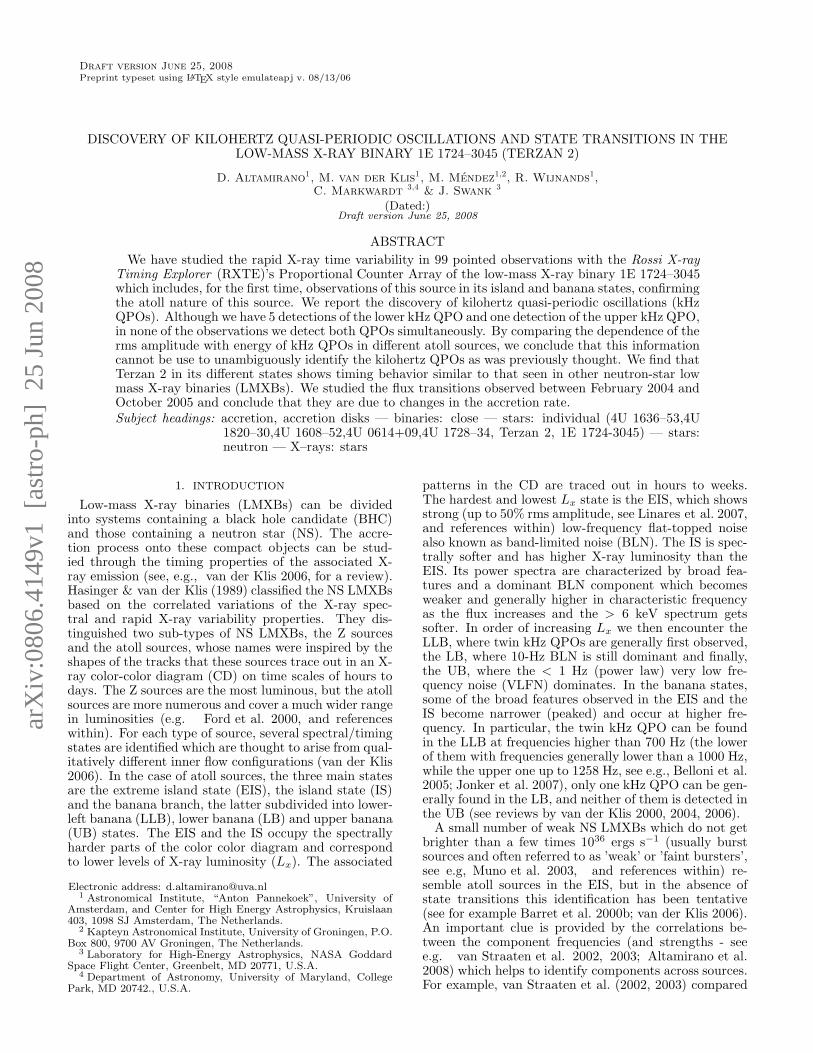
Fig. 1.— Above: PCA count rate obtained from the monitoringobservations of Terzan 2 (Monitoring observation of the galacticbulge - see Swank & Markwardt 2001). These data was used forthe study of the long-term variability (see Sections 2.4 & 3.8). Be-low: Terzan 2 intensity (Crab normalized - see Section 2) versustime of all pointed observations. These observations were used forthe study of the 0.1–1200 Hz X-ray variability (see Sections 2.2,3.4 & 3.3) except for the observation 90058-06-04-00, which ismarked with an arrow (see Section 3). The modified Julian date isdefined as MJD = Julian Date−2400000.5.

2.4. Search for quasi-periodic variations over days andmonths

Recently, Wen et al. (2006) have performed a system-atic search for periodicities in the light curves of 458

4

Time interval Duration Maximum Count Rate Flare No. of pointed obs.(MJD) (days) (cts/s/5PCU) label sampling the flare

∼ 53038 − 53071 33 ∼ 850 F1 7∼ 53127 − 53155 28 ∼ 950 F2 4∼ 53233 − 53250 17 ∼ 830 F3 2∼ 53493 − 53502 9 ∼ 450 F4 0∼ 53566 − 53602 36 ∼ 1150 F5 1∼ 53631 − 53651 20 ∼ 650 F6 0∼ 53934 − 53972 38 ∼ 865 F7 0

TABLE 1Data on the 6 flares observed until MJD 53667. See Section 3 for details. (The modified Julian date is defined as MJD =

Julian Date−2400000.5).

sources using data from the RXTE All Sky Monitor(ASM). Terzan 2 was not included in their analysis, prob-ably due to the fact that the ASM source average countrate is low: 2.05±0.01 count/s (the average of the errors– 1/n

∑

erri – is 0.8 count/s).Since the PCA galactic bulge monitoring

(Swank & Markwardt 2001) has observed the sourcefor more than 8 years, and the lowest detected sourcecount rate was 170 ± 5 counts/sec, this new data setprovides useful information to search for long termmodulations. Lomb-Scargle periodograms (Lomb 1976;Scargle 1982; Press et al. 1992) as well as the phase dis-persion minimization technique (PDM - see Stellingwerf1978) were used. The Lomb-Scargle technique is ideallysuited to look for sinusoidal signals in unevenly sampleddata. The phase dispersion minimization technique iswell suited to the case of non-sinusoidal time variationcovered by irregularly spaced observations.

3. RESULTS

3.1. The light curve

Figure 1 shows both the PCA monitoring lightcurveof the source (see upper panel and Swank & Markwardt2001) and the Crab normalized intensity (see lower paneland Section 2.1) of each pointed observation versustime (in units of modified Julian date MJD = JulianDate−2400000.5). In the rest of this paper, we will referas “quiet period” to that between MJD 51214 and 52945,and as “flaring period” between MJD 52945 and 53666.

During the quiet period, 333 monitoring measurementsof the source intensity and 85 pointed observations sam-ple the behavior of the source. The count rate slowly de-creases from an average of ∼ 300, to an average of ∼ 190counts/s/5PCU at an average rate of −0.059 ± 0.002count/s/day. In the flaring period, 7 flares sampledwith 201 monitoring observations were detected with thegalactic bulge scan. 14 pointed observations partiallysampled parts of 4 of these flares. In Table 1 we list ap-proximate dates at which the flux transitions occurred,the flare durations and the maximum count rates de-tected with the PCA. As mentioned in Section 2.4, themonitoring is done approximately once every three days;additional gaps in the data are present due to visibilitywindows. As of course we do not have details of flaresthat may have occurred during these gaps, the informa-tion in Table 1 is only approximate. In Figure 2 we showthe intensity of the source during the flaring period. Welabel the different flares F1, F2, F3, F4, F5, F6 and F7in order of time of occurrence.

We detected three Type I X-ray bursts. One was dur-ing the quiet-state observation 10090-01-01-021 and two

during the flaring-state observations 80138-06-06-00 and90058-06-02-00. A detailed study of these X-ray bursts aswell as a comparison to bursts observed in other sourcescan be found in Galloway et al. (2006).

0.02

0.03

0.04

0.05

0.06

0.07

0.08

0.09

53000 53200 53400 53600 53800 54000

Inte

nsity

(C

rab)

Time (MJD)

KLMNOPQR

����������������

����������������

��������������������

��������������������

������������

������������

Quiet state (EIS)

IS

LLB

LB

LLB

LB

F4

F5F6 F7

PCA lightcurveF1 F2 F3

QPOs

kHz

kHzQPOs

NO DATANO DATA NO DATA

Fig. 2.— Above: Intensity in units of the Crab Nebula of theobservations which were performed during the flare state. Thedifferent states are labeled (see Section 3.2). Arrows mark theobservations in which kHz QPOs were detected (see also Section 3.3and Table 3.3). Below: Intensity versus time showing the sevenflares. The data are the same as those of Figure 1.

3.2. Color diagrams; identification of states

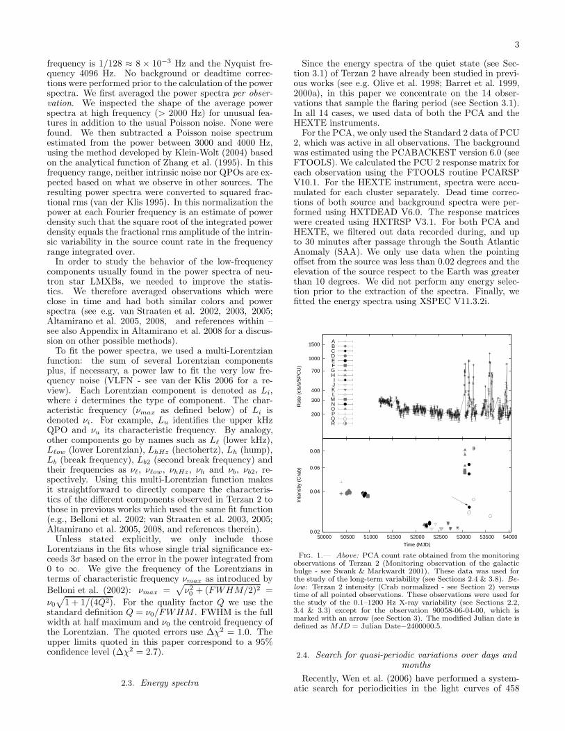
Figure 3 (top) shows the color-color diagram of the 99pointed observations. For comparison, we also includethe color-color diagram of the atoll source 4U 1608–52,which has been observed in all extreme island, islandand banana states (Figure 3, bottom). The similarity inshape suggests that Terzan 2 underwent state transitionsduring observations of the flares. Based on Figure 3we can identify the probable extreme island, islandand banana state with the hardest, intermediate andsoftest colors, respectively. Since partially sampledpatterns in the color color diagrams are not necessarilyunambiguous, (see review by van der Klis 2006), powerspectral analysis (below) is required to confirm theseidentifications. The extreme island state is sampledwith 85 pointed observations which are clumped in2 regions at similar hard colors but at significantlydifferent soft colors. We find 3 observations in theisland state. They sampled the lowest luminositysections of flares F2, F3 and F5 (see Figure 2). Thebanana state is sampled by 11 pointed observations:7 during F1, 3 during F2 and 1 during F3. Theidentifications above are strengthened by the similar-

5

ities in power spectral shapes between Terzan 2 andthose reported in other sources (van Straaten et al.2003; Di Salvo et al. 2001; van Straaten et al.2002; Di Salvo et al. 2003; van Straaten et al.2005; Linares et al. 2005; Altamirano et al. 2005;Migliari et al. 2005; Altamirano et al. 2008). In thefollowing sections we describe the power spectra in moredetail.

0.65

0.7

0.75

0.8

0.85

0.9

0.95

1

1.05

1.1

1.1 1.15 1.2 1.25 1.3 1.35 1.4

Har

d co

lor

(Cra

b)

Soft color (Crab)

EIS

IS

BS

Fig. 3.— Top: Hard color versus soft color normalized to Crab asexplained in Section 2. Different symbols represent the selectionsused for averaging the power spectra as explained in Section 2 andshown in Figure 6 (See Figure 1 for symbols). The arrow marksobservation 90058-06-04-00, which was excluded from interval N(see Section 3). Bottom: Hard color versus soft color normal-ized to Crab for the NS source 4U 1608–52. This source has beenobserved in all expected atoll states: extreme island state (EIS),island state (IS), lower left banana (LLB), lower banana (LB) andupper banana (UP). The similarity between both figures suggestthat Terzan 2 has been observed in similar states as 4U 1608–52.

3.3. kHz QPOs

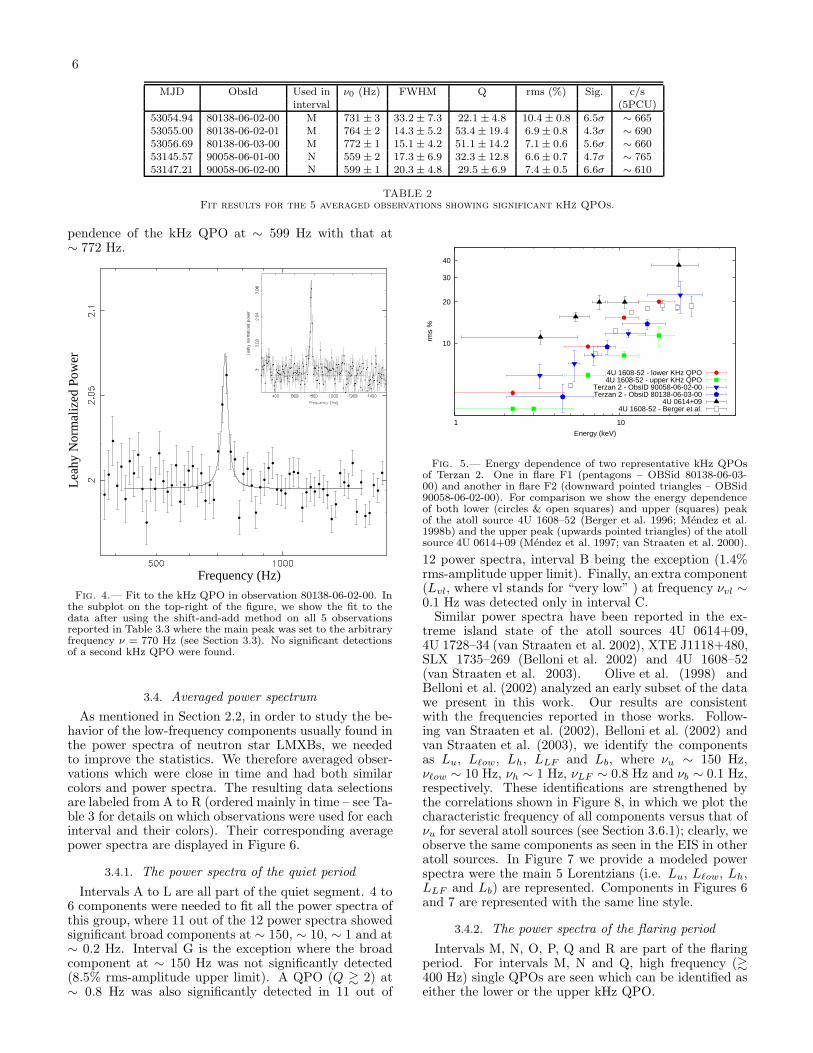
We searched each averaged observation’s power spec-trum for the presence of significant kHz QPOs at frequen-cies & 400 Hz. As reported in other works (Barret et al.1999; Belloni et al. 2002), during the quiet period thepower spectra of single averaged observations show sig-nificant power up to ∼ 300 Hz which is fitted withbroad (Q . 0.5) Lorentzians plus if necessary, one sharpLorentzian to account for LLF . During the flaring pe-riod, we found that several observations show power ex-cess above 400 Hz. For each observation we fitted the

averaged power spectra between 400 and 2000 Hz witha model consisting of one Lorentzian and a constant totake into account the QPO and Poisson noise, respec-tively. In 5 of the 14 observations that sample the flaringperiod, we detect significant QPOs, with single trial sig-nificances up to 6.5σ. In Table 3.3 we present the resultsof our fits and information on these observations. As canbe seen, the first three observations were performed dur-ing the rise of the first flare while the fourth and fifthobservations where done during the decay of the secondflare (see Figure 2). As can be seen in Table 3.3, thereare significant frequency variations. Unfortunately, dueto the sparse coverage of the flares and the fact that wecannot detect the QPO on shorter time scales than anobservation, no further conclusions are possible.

We do not significantly detect two simultaneous kHzQPOs in any of the 5 observations. In order to search fora possible second kHz QPO, we used the shift–and–addmethod as described by Mendez et al. (1998b). We firsttried to trace the detected kilohertz QPO using a dynam-ical power spectrum (e.g. see figure 2 in Berger et al.1996) to visualize the time evolution of the QPO fre-quency, but the signal was too weak to be detected ontimescales shorter than the averaged observation. There-fore, for each observation we used the fitted averagedfrequency (see Table 3.3) to shift each kilohertz QPOto the arbitrary frequency of 770 Hz. Next, the shifted,aligned, power spectra were averaged. The average powerspectrum was finally fitted in the range 300–2048 Hz soas to exclude the edges, which are distorted due to theshifting method. To fit the averaged power spectrum, weused a function consisting of a Lorentzian and a constantto fit the QPO and the Poisson noise, respectively. Westudied the residuals of the fit, but no significant powerexcess was present apart from the 770 Hz feature. InFigure 4 we show the fitted kHz QPO for observation80138-06-02-00 (no shift and add was applied) and theshifted-and-added kHz QPO detected with the methodmentioned above. Since it is known that the kHz QPOsbecome stronger at higher energies (e.g. Berger et al.1996; Mendez et al. 1998a; van der Klis 2000, and refer-ences within), we repeated the analysis described above(which was performed on the full PCA energy range), us-ing only data at energies higher than ∼ 6 keV or higherthan ∼ 10 keV. Again, no significant second QPO waspresent. It is important to note that this method canproduce ambiguous results as we cannot be sure we arealways shifting the same component (either Lu or Lℓ).We also tried different subgroups, i.e. adding only twoto three different observations, but found the same re-sults.

To investigate the energy dependence of the kHzQPOs, we divided each power spectrum into 3, 4 or 5 en-ergy intervals in order to have approximately the samecount rate in all the intervals. We then produced thepower spectrum as described in Section 2 and refittedthe data where both frequency and Q were fixed to thevalues obtained for the full energy range (see Table 3.3).In Figure 5 we show the results for the representative kHzQPOs in flares F1 and F2 (observations 80138-06-03-00and 90058-06-02-00, respectively). Similarly to what isobserved in other sources, the fractional rms amplitudeof the kHz QPOs increases with energy. The data showthat there is no significant difference in the energy de-

6

MJD ObsId Used in ν0 (Hz) FWHM Q rms (%) Sig. c/sinterval (5PCU)

53054.94 80138-06-02-00 M 731 ± 3 33.2 ± 7.3 22.1 ± 4.8 10.4 ± 0.8 6.5σ ∼ 66553055.00 80138-06-02-01 M 764 ± 2 14.3 ± 5.2 53.4 ± 19.4 6.9 ± 0.8 4.3σ ∼ 69053056.69 80138-06-03-00 M 772 ± 1 15.1 ± 4.2 51.1 ± 14.2 7.1 ± 0.6 5.6σ ∼ 66053145.57 90058-06-01-00 N 559 ± 2 17.3 ± 6.9 32.3 ± 12.8 6.6 ± 0.7 4.7σ ∼ 76553147.21 90058-06-02-00 N 599 ± 1 20.3 ± 4.8 29.5 ± 6.9 7.4 ± 0.5 6.6σ ∼ 610

TABLE 2Fit results for the 5 averaged observations showing significant kHz QPOs.

pendence of the kHz QPO at ∼ 599 Hz with that at∼ 772 Hz.

Lea

hy N

orm

aliz

ed P

ower

Frequency (Hz)

Fig. 4.— Fit to the kHz QPO in observation 80138-06-02-00. Inthe subplot on the top-right of the figure, we show the fit to thedata after using the shift-and-add method on all 5 observationsreported in Table 3.3 where the main peak was set to the arbitraryfrequency ν = 770 Hz (see Section 3.3). No significant detectionsof a second kHz QPO were found.

3.4. Averaged power spectrum

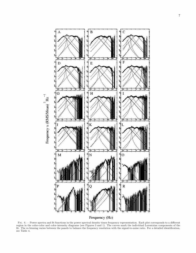
As mentioned in Section 2.2, in order to study the be-havior of the low-frequency components usually found inthe power spectra of neutron star LMXBs, we neededto improve the statistics. We therefore averaged obser-vations which were close in time and had both similarcolors and power spectra. The resulting data selectionsare labeled from A to R (ordered mainly in time – see Ta-ble 3 for details on which observations were used for eachinterval and their colors). Their corresponding averagepower spectra are displayed in Figure 6.

3.4.1. The power spectra of the quiet period

Intervals A to L are all part of the quiet segment. 4 to6 components were needed to fit all the power spectra ofthis group, where 11 out of the 12 power spectra showedsignificant broad components at ∼ 150, ∼ 10, ∼ 1 and at∼ 0.2 Hz. Interval G is the exception where the broadcomponent at ∼ 150 Hz was not significantly detected(8.5% rms-amplitude upper limit). A QPO (Q & 2) at∼ 0.8 Hz was also significantly detected in 11 out of

10

20

30

40

1 10rm

s %

Energy (keV)

4U 1608-52 - lower KHz QPO4U 1608-52 - upper KHz QPO

Terzan 2 - ObsID 90058-06-02-00Terzan 2 - ObsiD 80138-06-03-00

4U 0614+094U 1608-52 - Berger et al.

Fig. 5.— Energy dependence of two representative kHz QPOsof Terzan 2. One in flare F1 (pentagons – OBSid 80138-06-03-00) and another in flare F2 (downward pointed triangles – OBSid90058-06-02-00). For comparison we show the energy dependenceof both lower (circles & open squares) and upper (squares) peakof the atoll source 4U 1608–52 (Berger et al. 1996; Mendez et al.1998b) and the upper peak (upwards pointed triangles) of the atollsource 4U 0614+09 (Mendez et al. 1997; van Straaten et al. 2000).

12 power spectra, interval B being the exception (1.4%rms-amplitude upper limit). Finally, an extra component(Lvl, where vl stands for “very low” ) at frequency νvl ∼

0.1 Hz was detected only in interval C.Similar power spectra have been reported in the ex-

treme island state of the atoll sources 4U 0614+09,4U 1728–34 (van Straaten et al. 2002), XTE J1118+480,SLX 1735–269 (Belloni et al. 2002) and 4U 1608–52(van Straaten et al. 2003). Olive et al. (1998) andBelloni et al. (2002) analyzed an early subset of the datawe present in this work. Our results are consistentwith the frequencies reported in those works. Follow-ing van Straaten et al. (2002), Belloni et al. (2002) andvan Straaten et al. (2003), we identify the componentsas Lu, Lℓow, Lh, LLF and Lb, where νu ∼ 150 Hz,νℓow ∼ 10 Hz, νh ∼ 1 Hz, νLF ∼ 0.8 Hz and νb ∼ 0.1 Hz,respectively. These identifications are strengthened bythe correlations shown in Figure 8, in which we plot thecharacteristic frequency of all components versus that ofνu for several atoll sources (see Section 3.6.1); clearly, weobserve the same components as seen in the EIS in otheratoll sources. In Figure 7 we provide a modeled powerspectra were the main 5 Lorentzians (i.e. Lu, Lℓow, Lh,LLF and Lb) are represented. Components in Figures 6and 7 are represented with the same line style.

3.4.2. The power spectra of the flaring period

Intervals M, N, O, P, Q and R are part of the flaringperiod. For intervals M, N and Q, high frequency (&400 Hz) single QPOs are seen which can be identified aseither the lower or the upper kHz QPO.

7

Fig. 6.— Power spectra and fit functions in the power spectral density times frequency representation. Each plot corresponds to a differentregion in the color-color and color-intensity diagrams (see Figures 3 and 1). The curves mark the individual Lorentzian components of thefit. The re-binning varies between the panels to balance the frequency resolution with the signal-to-noise ratio. For a detailed identification,see Table 4.

8

Interval A

Observation Soft color (Crab) Hard color (Crab) Intensity (Crab)

10090-01-01-000 1.3615 ± 0.0017 1.0760 ± 0.0013 0.0389 ± 0.000110090-01-01-001 1.3508 ± 0.0019 1.0761 ± 0.0014 0.0384 ± 0.000110090-01-01-00 1.3619 ± 0.0019 1.0757 ± 0.0015 0.0384 ± 0.000110090-01-01-020 1.3783 ± 0.0021 1.0781 ± 0.0016 0.0386 ± 0.000110090-01-01-021 1.4435 ± 0.0019 0.9846 ± 0.0013 0.0468 ± 0.000110090-01-01-022 1.3638 ± 0.0017 1.0788 ± 0.0013 0.0387 ± 0.000110090-01-01-02 1.3723 ± 0.0039 1.0801 ± 0.0029 0.0389 ± 0.0001

Interval B

20170-05-01-00 1.3501 ± 0.0075 1.0660 ± 0.0058 0.0383 ± 0.000120170-05-02-00 1.3440 ± 0.0077 1.0492 ± 0.0059 0.0384 ± 0.000120170-05-03-00 1.3498 ± 0.0076 1.0541 ± 0.0058 0.0389 ± 0.000120170-05-04-00 1.3449 ± 0.0073 1.0632 ± 0.0056 0.0394 ± 0.000120170-05-05-00 1.3492 ± 0.0071 1.0703 ± 0.0055 0.0398 ± 0.000120170-05-06-00 1.3392 ± 0.0072 1.0650 ± 0.0056 0.0394 ± 0.000120170-05-07-00 1.3465 ± 0.0072 1.0726 ± 0.0055 0.0393 ± 0.000120170-05-08-00 1.3295 ± 0.0071 1.0605 ± 0.0056 0.0382 ± 0.000120170-05-09-00 1.3398 ± 0.0070 1.0704 ± 0.0054 0.0389 ± 0.000120170-05-10-00 1.3163 ± 0.0064 1.0687 ± 0.0051 0.0387 ± 0.000120170-05-11-00 1.3601 ± 0.0071 1.0714 ± 0.0054 0.0400 ± 0.000120170-05-12-00 1.3365 ± 0.0074 1.0747 ± 0.0058 0.0399 ± 0.000120170-05-13-00 1.3532 ± 0.0070 1.0721 ± 0.0053 0.0409 ± 0.000120170-05-14-00 1.3215 ± 0.0076 1.0768 ± 0.0061 0.0407 ± 0.000120170-05-15-00 1.3417 ± 0.0070 1.0658 ± 0.0054 0.0394 ± 0.000120170-05-16-00 1.3398 ± 0.0081 1.0669 ± 0.0062 0.0398 ± 0.000120170-05-17-00 1.3290 ± 0.0072 1.0832 ± 0.0057 0.0386 ± 0.000120170-05-18-00 1.3318 ± 0.0086 1.0682 ± 0.0067 0.0392 ± 0.000120170-05-19-00 1.3336 ± 0.0068 1.0667 ± 0.0053 0.0395 ± 0.000120170-05-20-00 1.3309 ± 0.0069 1.0599 ± 0.0054 0.0397 ± 0.0001

TABLE 3Observations used for the timing analysis. The colors and intensity are corrected by dead time and normalized to the

Crab Nebula (see Section 2). The complete table can be obtained digitally from ApJ.

9Fr

eque

ncy

x (R

MS/

Mea

n)

Hz

−1

2

Frequency (Hz)

L

L

L L Lb

LF

hu ow

Fig. 7.— Example of the typical power spectra of the quietperiod. The main 5 Lorentzians are Lu, Lℓow, Lh, LLF and Lb

(see Section 3.4.1).

The kHz QPOs in interval M and N correspond to theaverages of significant QPOs observed in single observa-tions. As seen in Table 3.3, the characteristic frequencyof the kHz QPOs averaged in each of the two intervals arewithin a range of 50 Hz. By our averaging method we areaffecting the Q value of the kHz QPOs but improving thestatistics for measuring the characteristics of the featuresat lower frequencies (see Appendix in Altamirano et al.2008, for a discussion on this issue).

Interval Q is an average of three single observations(see Table 3) that individually do not show significantQPOs ( Q > 2) at high frequencies although low-Q powerexcess can be measured. Lh in interval Q is only 2.6σsignificant (single trial) but required for a stable fit.

Interval O shows a broad component at 30.5 ± 6.3 Hzand a 3.3% rms low-frequency noise. In this case,the very low frequency noise was fitted with a broadLorentzian because a power law gave an unstable fit.The excess of power at ν & 1000 Hz is less than 3σsignificant. Interval P shows a power spectrum with apower-law low frequency noise, and two Lorentzian com-ponents at frequencies 15.5 ± 1.6 and 30.5 ± 6.3 Hz (seeFigure 6). In this case the high χ2/dof = 218/163 re-veals that the Lorentzians do not satisfactorily fit thedata. As can be seen in Figure 6, there is a steep de-cay of the power above ν ∼ 35 Hz and power excess at∼ 70 Hz. A fit with three Lorentzians becomes unsta-ble. To further investigate this, we refitted the powerspectrum using instead two Gaussians and one powerlaw to fit the power at ν . 40 Hz, and one Lorentzianto fit the possible extra component at ∼ 70 Hz. Thesteeper Gaussian function better fits the steep power de-cay than the Lorentzians. In this fit, with three morefree parameters, we obtain a χ2/dof = 188/160, and theLorentzian at 69.1±2.6 Hz becomes 3.4σ single-trial sig-nificant. This power spectrum is very similar to those re-ported by Migliari et al. (2004, 2005) and Migliari et al.(2005) for the atoll sources 4U 1820–30 and Ser X-1, re-

0.1

0.5

1

5

10

20

30 40 50

70

100

200

300

1000

100 200 300 500 700 1000

ν max

(H

z)

νu (Hz)

Lb2Lb

LhHzLh

LlowLl

Terzan 2 (this paper)

Fig. 8.— The characteristic frequencies νmax of the var-ious power spectral components plotted versus νu. The greysymbols mark the atoll sources 4U 0614+09, 4U 1728–34(van Straaten et al. 2002), 4U 1608–52 (van Straaten et al. 2003),Aql X-1 (Reig et al. 2004) and 4U 1636–53 (Altamirano et al.2008) and the low luminosity bursters Terzan 2 (previous results),GS 1826–24 and SLX 1735–269 (van Straaten et al. 2005, but alsosee Belloni et al. 2002). The black bullets mark our results forTerzan 2. Note that we only plot the results for Intervals A-N andQ (note that as mentioned in Section 3.6.1, the points for intervalsM and N (νu > 800 Hz) were plotted under the assumption thatνu = νℓ + 300 Hz). For intervals O, P and R no kHz QPOs weredetected (see Section 3.4).

spectively. Besides the similarity in shape of the powerspectrum, it is interesting to note that in both cases theseauthors found a best fit with components at similar fre-quencies to the ones we observe in Terzan 2 and whichthey interpreted as νb, νh and νhHz . This coincidencesuggests that the sources were in very similar states. Toour knowledge, no systematic study of this state has beenreported as yet.

Interval R consists of only one observation (90058-06-05-00) of ∼ 1.4 ksec of data. In addition to a power lawwith index α = 3.1 ± 0.7, we detect one Lorentzian at68.5± 7.2 Hz. Its frequency is rather high if we compareit with the other power spectra presented in this paperand even when compared with results in other sources(see Figure 8). This result might be due to blendingof components due to the low statistics present in thispower spectrum.

From the 99 pointed observations, only observation90058-06-04-00 was not included in any of the averagesdescribed above. The averaged colors of this observation

10

are similar to those of Interval N (observations 90058-06-01-00, 90058-06-02-00) but the power spectrum doesnot show a significant QPO at ≃ 560 Hz and can befitted with a single Lorentzian at νmax = 23.6 ± 3.3 Hz,Q = 0.5±0.2 and rms= 13.2±0.9%. The residuals of thefit show excess power at ≃ 800 Hz but no significant kHzQPO. Although the colors of observation 90058-06-04-00are similar from those of interval N, the power spectrumis different. Because of this, we refrained from averaging90058-06-04-00 into interval N.

0

5

10

15

20

25

30

35

40

0.65 0.7 0.75 0.8 0.85 0.9 0.95 1 1.05 1.1

rms

(%)

in th

e 0.

1-10

00 H

z ra

nge

Hard Color (Crab)

Fig. 9.— Fractional rms (%) amplitude versus hard color normal-ized to the Crab Nebula as explained in Section 2. The light-greysquares represent the data of the “quiet” state while the dark-greycircles represent the data for the “flare” state. The black circlesrepresent the upper limit (∆χ2 = 2.7) for the observations 80138-06-05-00 and 80138-06-06-00 which also partially sampled the flarestates.

3.5. Integrated power

In order to study the rms amplitude dependence oncolor and intensity, we calculated the average integralpower per observation between 0.1 and 1000 Hz. In Fig-ure 9 we show the 0.01–1000 Hz averaged rms amplitude(%), of each of the 99 observations, versus its averagehard color. The observations which sample the islandand banana state correlate with the averaged hard color.This type of correlation has been already observed inblack hole candidates and neutron star systems (see e.g.Homan et al. 2001). At colors harder than 1.0, there aretwo clumps (grey squares in Figure 9) which can also beseen in the color-color diagram (Figure 3). They bothcorrespond to observations of the extreme island state(quiet state) of the source. As we show in Figure 6, thepower spectral shape remains approximately the samewith time. However, for a given hard color, the total rmsamplitude can change up to ≃ 30%. No correlation withtime, intensity or soft color was found and these changesare seen within a small range in intensity (less than 4mCrab). Similar results are also observed when the rmsamplitude is calculated in the 0.01–300 Hz range.

3.6. Comparing Terzan 2 with other LMXBs

3.6.1. The flaring period

In Figure 10 we plot the frequency correlations betweenLLF and Lℓ reported by Psaltis & Chakrabarty (1999)and updated by Belloni et al. (2002). In Figure 8 we

plot the characteristic frequency of all components ver-sus that of νu for the atoll sources 4U 0614+09, 4U 1728–34, 4U 1608–52, 4U 1636–53 and Aql X-1 and the twolow luminosity bursters GS 1826–24 and SLX 1735–269 (van Straaten et al. 2002, 2003; Reig et al. 2004;Altamirano et al. 2008). Using these correlations toidentify the highest frequencies we observe (in inter-vals M, N & Q) as either νu or νℓ presents a prob-lem. Both interpretations give consistent results sincethe correlations observed are complex when νu & 600 Hz(van Straaten et al. 2005).

0.01

0.1

1

10

100

1 10 100 1000

ν LF

νl

PBK99-BPK02Terzan 2 (This paper)

Fig. 10.— PBK relation after Psaltis & Chakrabarty (PBK99- 1999) and Belloni et al. (BPK02 - 2002). The black squares atνLF < 10 Hz represent the data of Intervals A and C–L while theblack squares at νLF > 20 Hz represent the data of Intervals Mand N. In Interval B we do not detect LLF and in intervals Q–Rwe do not detect Lℓ.

In recent work, Barret et al. (2005a,b,c) have system-atically studied the variation of the frequency, rms am-plitude and the quality factor Q of the lower and upperkHz QPOs in the low-mass X-ray binaries 4U 1636–536,4U 1608–52 and 4U 1735–44. Although Q depends on thefrequency of the component, these authors show that Qℓ

is always above ∼ 30, while Qu is generally below ∼ 25.By comparing our results for the kHz QPOs with those ofBarret et al. (2005a,b,c), we find that the 5 QPOs listedin Table 3.3 (and averaged in intervals M and N) are rel-atively high-Q and hence consistent with being Lℓ, butalso still consistent with being Lu. The quality factor ofthe kHz QPO found in interval Q is low (2.4 ± 0.6) andhence this kHz QPO is probably Lu.

In Figure 11 we plot the fractional rms amplitudeof all components (except LLF ) versus νu for the 4atoll sources 4U 0614+09, 4U 1728–34, 4U 1608–52,4U 1636–53. With respect to the kHz QPO identifi-cation, the interpretation that we found Lℓ in intervalN is strengthened by the rms amplitudes of the twolow-frequency components found in the averaged powerspectrum. If the QPO we observe is not Lℓ but Lu,then the low frequency QPO pairs can be identified aseither Lh-Lb or Lb-Lb2. For νu = 586.1 ± 6.6, thepair Lh-Lb is not consistent with what we observe forother atoll sources (Figure 11), since Lb is not seen withrms amplitude as low as 3.9+0.8

−0.5%. The pair Lb-Lb2

is not consistent with the data either, since Lb2 is al-ways observed at νu & 800 Hz. If the QPO is Lℓ, then

11

based on what we observe in other well-studied sources(Mendez et al. 1998b; Mendez & van der Klis 1999;Di Salvo et al. 2003; Barret et al. 2005b; van der Klis2006; Mendez & Belloni 2007) we expect that the fre-quency difference between kHz QPOs is ∆ν = νu − νℓ ≃

300 and therefore νu ≃ νℓ + 300 ≃ 586 + 300 ≃ 886 Hz.Under this assumption (i.e. ∆ν ≃ 300) and by usingthe same reasoning as above, then only the pair Lb-Lb2

is consistent with the data. In the case of interval M,only one component is found at low frequencies withan rms amplitude of 6.4 ± 0.6%. This result is consis-tent with several interpretations when compared withthe data shown in Figure 11. Therefore, for interval Mwe cannot improve confidence in the identification of thekHz QPO using Figure 11.

In Figures 8, 10 & 11 we have plotted the data forTerzan 2 based on the identifications above. As discussedlater in this paper, such identifications need to be con-firmed.

3.6.2. The quiet period

In Figure 11 we show that the rms amplitude ofLu, Lℓow, Lh and Lb in Terzan 2 approximatelyfollow the trend observed for other sources. SincePsaltis & Chakrabarty (1999) interprets Lℓow and Lℓ asthe same component in different source states, in Fig-ure 11 we plot the data for both components together.Of course, in Figure 11 and Figure 8 as well, thereis the well-known gap between these two components.Regarding lower frequency components, the point in-side the circle represents our result for Lvl in intervalC, which is the weakest component found in the EISof Terzan 2. We plotted our results with those forLb2. This component might be related with the VLFNLorentzian (see Schnerr et al. 2003; Reerink et al. 2005).Altamirano et al. (2008) showed that the rms amplitudeof LLF of several atoll sources does not correlate with νu.There is also no evidence for a correlation in the case ofTerzan 2 (not plotted).

3.7. Luminosity estimates from spectral fitting

We fitted the PCA and the two cluster’s HEXTE spec-tra simultaneously using a model consisting of a blackbody to account for the soft component of the spec-tra and a power law to account for the hard compo-nent. In some cases, it was necessary to add a Gaus-sian to take into account the iron Kα line (6.4 keV, seee.g. White et al. 1986). We ignore energies below 2.5and above 25keV for the PCA spectra, and below 20and above 200 keV for the HEXTE spectra (see e.g.Barret et al. 2000a). In most cases, it is not possi-ble to well constrain the interstellar absorption nH ifwe lack spectral information below 2.5 keV. We there-fore opted to fix nH to the value nH = 1.2 · 1022

H atoms cm−2 (in the Wisconsin cross section wabsmodel – see Morrison & McCammon 1983 ) based onprevious ASCA/BeppoSAX results (Olive et al. 1998;Barret et al. 1999, 2000a).

Assuming a distance of 6.6 kpc, we found that all14 observations have luminosities between ∼ 0.4 and∼ 1.35 × 1037 erg s−1 in the energy range 2–20 keV.We also found that at high energies (20–200 keV) the lu-minosities of most observations were less than 0.09×1037

erg s−1. The exceptions are the three observations which

sample the island state, which show 20–200 keV lumi-nosities of ∼ 0.16, ∼ 0.23 and ∼ 0.29 × 1037 erg s−1

(observations 90058-06-03-00, 90058-06-06-00 and 91050-07-01-00, respectively). This may be compared with ob-servations of the brightest interval of the quiet period ofTerzan 2, which have averaged luminosities L1−20keV =0.81×1037 erg s−1 and L20−200keV = 0.48×1037 erg s−1

(Barret et al. 2000a). Clearly, in between the flares theluminosity can drop to similarly low values as in the quietperiod. This is consistent with the lightcurve we showin Figure 1. We note that the observations studied byBarret et al. (2000a) correspond to MJDs 50391− 50395(November 4-8, 1996) and sample the brightest part ofthe quiet period of this source observed with RXTE (seeFigure 1).

We are particularly interested in the luminosity atwhich the kHz QPOs are detected in Terzan 2 comparedwith other sources. Ford et al. (2000) have measured si-multaneously the properties of the energy spectra andthe frequencies of the kHz QPOs in 15 low-mass X-raybinaries covering a wide range of X-ray luminosities. Theobservations of intervals M and N (see Table 1) have av-erage luminosities L2−50keV /Ledd between 0.025 and 0.04(where Ledd = 2.5 × 1038 erg s−1). The three observa-tions that sample the island state (interval Q) have aver-age luminosity L2−50keV /Ledd ≃ 0.02. This means thatduring the flares, Terzan 2 shows kHz QPOs at similarluminosities to the atoll sources Aql X-1, 4U 1608–52,4U 1702–42 and 4U 1728–34 (see figure 1 in Ford et al.2000).

3.8. Lomb Scargle Periodograms

During the quiet period (51214–52945 MJD), we foundno significant periodicities using either the Lomb-Scargleor the PDM techniques in the full data set nor in sub-intervals.

As shown in Figure 1, the flares seem to occur ev-ery ∼ 60 − 100 days. Both Lomb-Scargle and the PDMtechniques confirm this with a significant signal of pe-riod P ∼ 90.55 days. In Figure 12 we show the PCAlightcurve (top) versus a 20-bin 90.55 days period foldedlightcurve (bottom). The folded lightcurve matches theoccurrence of most of the flares. However, it is clearthat the flares are not strictly periodic. For example, F3seems to occur later and F6 occur earlier than expected.Furthermore, it is not possible to say if F7 is an early orlate flare, or even a blend of two flares (we observed asmall flare which peaked at ≃ 53926 MJD, followed by abig one which peaked at ≃ 53958 MJD). Although thereare gaps in the data, Figure 12 suggests that some flaresdo not occur at all (see arrow in this figure).

4. DISCUSSION

4.1. Contamination by a second source in the same fieldof view?

As shown in Figure 1, the luminosity of the sourceslowly decreases with time during the quiet period51214–52945 MJD. Although the rms amplitude changesup to 30% (see Figure 9), the X-ray timing characteris-tics are very similar (see Interval A to L in Figure 6).During the 53000–53700 MJD period, the source showsflares which show different X-ray timing characteristicsconsistent with the island and banana states observed

12

5

10

15

20

RM

S o

f Lb2

(%

)

4U 1728--344U 1608--524U 0614+094U 1636--53

Terzan 2

5

10

15

20

RM

S o

f Lb

(%)

5

10

15

20

RM

S o

f Lh

(%)

5

10

15

20

RM

S o

f LhH

z (%

)

200 400 600 800 1000 1200

5

10

15

20

RM

S o

f Ll (

%)

νu (Hz)

5

10

15

20

200 400 600 800 1000 1200

RM

S o

f Lu

(%)

νu (Hz)

Fig. 11.— The fractional rms amplitude of all components (except LLF ) plotted versus νu. The symbols are labeled in the plot. Thedata for 4U 1728–34, 4U 1608–52 and 4U 0614+09 were taken from van Straaten et al. (2005). The data for 4U 1636–53 were taken fromAltamirano et al. (2008). Note that for LhHz and Lh of 4U 1608–52, the 3 triangles with vertical error bars which intersect the abscissarepresent 95% confidence upper limits (see van Straaten et al. (2003) for a discussion). The points inside the circle represent our results forLvl while the points inside the square represent results for Llow (see Section 4 for a discussion). Note that as mentioned in Section 3.6.1,the points for intervals M and N (νu > 800 Hz) were plotted under the assumption that νu = νℓ + 300 Hz.

53000 53200 53400 53600 53800 54000

Rel

ativ

e co

unt r

ate

Time (MJD)

F1F2

F3

F4

F5

F6

F7

Fig. 12.— The PCA monitoring observation lightcurve ofTerzan 2 in the time interval 53013–54050 MJD (above) versusa series of folded light curves with period of 90.55 days (below).The black arrow shows the position of a possible missed flare (seeSection 4.3

in other atoll sources (see e.g. van Straaten et al. 2003,2005; Belloni et al. 2002; Altamirano et al. 2005, 2008).A possible mechanism of the observed flux variations inTerzan 2 could be the emergence of a second X-ray sourcein this globular cluster unresolved by the 1◦ (FWHM)field of view of the PCA. If two sources are observed si-multaneously with RXTE, then we would expect to seepower spectra which are a combination of the intrinsictime variability of both sources.

To further investigate this, we compared the absoluterms amplitude that we observe both in the quiet andflaring states. Observation 80105-10-01-00 is the last ob-servation performed during the quiet period from whichwe measured an average source countrate of ∼ 200 counts/ second. The integrated power between 7.8 · 10−3 and1 Hz is (3.4 ± 2)10−2, which corresponds to a fractionalrms amplitude of ∼ 18 ± 0.6%, i.e. an absolute rms am-plitude of 36 ± 1 counts/second.

Observation 80138-06-01-00 is the first observation per-formed during the flaring state. Its average countrate is∼ 740 counts / second and the absolute rms amplitudein the 0.0078 − 1 Hz range is 21.4 ± 4.4 counts/second

13

(2.9 ± 0.6% fractional rms amplitude). Clearly, theabsolute rms amplitudes are different when comparingquiet and flaring periods. If we repeat the analysisusing the second RXTE observation during the flaringstate (80138-06-02-00), the discrepancy is higher. Thisobservation has an average source countrate of ∼ 405counts/second and the upper limit for the absolute rmsamplitude in the 7.810−3

− 1 Hz frequency range is 5counts/second.

Given the characteristics of the power spectra, flarescannot be explained by assuming that another sourcehas emerged, unless Terzan 2 turned off at the same timethat the other X-ray source turned on, which is unlikely.Therefore, we conclude that the flux transitions are in-trinsic to the only low mass X-ray binary detected in theglobular cluster Terzan 2: 1E 1724–30 (Revnivtsev et al.2002).

4.2. The kilohertz QPOs, different states and theirtransitions

The results presented in this paper show that the lowluminosity source 1E 1724–3045 in the globular clusterTerzan 2 can be identified as an atoll source. This is thefirst time a source previously classified as weak burstsource (see e.g, Belloni et al. 2002; van Straaten et al.2003, and references within) showed other states thanthose of the extreme island state, confirming previoussuggestions that these sources are atoll sources. We haveidentified the new states as the island and banana statesbased on comparisons between color color diagrams ofdifferent sources and the characteristics of the powerspectra. We have detected at least one of the the kHzQPOs, and as explained in Sections 3.4.2 and 3.3, in 5cases we may be detecting the lower kHz QPO (intervalsM and N – see also Table 3.3) and in one case the upperone (interval Q). No simultaneous twin kHz QPOs weredetected within any of the 14 observations that samplethe flares. Future observations of flares will allow us toconfirm these identifications and might allow us to detectboth kHz QPOs simultaneously.

We found that the frequencies of the various compo-nents in the power spectra of Terzan 2 followed previ-ously reported relations (Figures 8 and 10). Terzan 2 isa particularly important source in the context of thesefrequency correlations because it is one of the few neu-tron star sources that has been demonstrated to showpower spectral features that reach frequencies as lowas ≃ 0.1 Hz, which is uncommon for neutron star lowmass X-ray binaries, but not for black holes. Our re-sults demonstrate that in each of the flares, Terzan 2 un-dergoes flux transitions that, if directly observed, wouldprobably allow us to resolve current ambiguities in theidentification of components, such as the case of Lℓow

component in atoll sources. This component is inter-preted by some authors as a broad lower kHz QPO atvery low frequencies (see Psaltis & Chakrabarty 1999;Nowak 2000; Belloni et al. 2002) which becomes peakedat higher frequencies, while other authors interpret Lℓ

and Lℓow as different components (see e.g. discussionin van Straaten et al. 2003). Another example is theidentification of the upper kHz QPO at low frequen-cies. van Straaten et al. (2003) have suggested that thebroad component observed at ≃ 150 Hz in the EISof atoll sources becomes the peaked upper kHz QPO

Lu. These authors based their interpretation on thefrequency correlations shown in Figure 8. Nevertheless,as van Straaten et al. (2003) argue, these identificationsshould be taken as tentative. One way to confirm the linkbetween them would be to observe the gradual transfor-mation from one to another one.

During the time between flares, the source shows inten-sities similar to those measured before the quasi-periodicflares started. Unfortunately there are no observationsduring those intervals, but we expect that then Terzan 2shows X-ray variability similar to that reported in inter-vals A–L. If this is the case, the state transition betweenthe extreme island state and the island state should beobservable in observations at the beginning or at theend of each flare. Given the relatively gradual and pre-dictable transitions, Terzan 2 becomes the best sourceknown up to now to study these important transitions.

4.3. On the ∼ 90 days flare recurrence

The quasi-periodic variations over days and monthsobserved in some LMXBs X-ray light-curves are gener-ally associated with the possible precession period of atilted accretion disk or alternatively long term periodicvariations in the accretion rate or periodic outbursts ofX-ray transients. Some examples are the ≃ 35 cycle inHer X-1 which is thought to be caused by a varying ob-scuration of the neutron star by a tilted-twisted precess-ing accretion disc; the ≃ 170 days accretion cycle of theatoll source 4U 1820–30, (Priedhorsky & Terrell 1984a;Simon 2003); the 122-125 day cycle in the outbursts ofthe recurrent transient Aql X-1 (Priedhorsky & Terrell1984b; Kitamoto et al. 1993). Understanding the mech-anisms that trigger the long-term variability associatedwith variations in the accretion rate of LMXBs can allowus to better predict, within each source, when the statetransitions occur. This is useful because these transitionsare usually fast and therefore difficult to observe.

The power spectra of our observations of Terzan 2 dur-ing the flaring confirm that the source undergoes EIS-IS-LLB-LB-UB state transitions, as observed in other neu-tron star atoll systems (and not as seen for Z-sources,see reviews by van der Klis 2004, 2006, and referenceswithin). As the source increased in X-ray luminosity,we found that the components in the power spectra in-creased in frequency which is consistent with the inter-pretation that the accretion disk is moving inwards to-ward the compact object. Therefore, the flaring with av-erage 90 days period is most probably an accretion cycle.We note that the modulation of the light-curve could berelated to the orbital period of the system or set by theprecession of a tilted disk. However, the mechanisms in-volved in those interpretations are very unlikely to affectthe frequency of the kHz QPOs.

If the flares are explained as an accretion cycle, thenit is puzzling why the source underwent a smooth de-crease of Lx for ≃ 8 years before it started to show theflares. Terzan 2 may not be the only source that showsthis kind of behavior. For example, KS 1731–260 is alow-luminosity burster that has shown a high Lx phase,during which Revnivtsev & Sunyaev (2003) reported apossible ≃ 38 days period, and a low Lx phase, duringwhich much stronger variability was observed (which wasdescribed as red noise). After its low Lx phase, KS 1731–260 has turned into quiescence (Wijnands et al. 2002b,a).

14

In Figure 13 we show the bulge scan light curve of thesource during the low Lx phase. At MJD ∼ 51550 thesource reached very low intensities, then flared up againfor & 250 days to finally turn into quiescence. The lowluminosities are confirmed by the ASM light curve (notplotted). Recently, Shih et al. (2005) reported that thepersistent atoll source 4U 1636–53 has also shown a pe-riod of high Lx followed by a period of low Lx. Duringhigh Lx, no long-term periodicity was found, but a highlysignificant ≃ 46 days period was observed after its Lx de-cline.

These similar patterns of behavior might point towardsa common mechanism, which then must be unaffected bythe intrinsic differences between these sources.

For example, while Terzan 2 remained with ap-proximately constant luminosity in its extreme islandstate for ≃ 8 years before showing long term period-icities, 4U 1636–53 and KS 1731–260 were observedwith variable luminosity and in different states, includ-ing the banana state in which the kHz QPOs werefound (see e.g. Wijnands et al. 1997 and Shih et al.2005 for 4U 1636–53 and Wijnands & van der Klis 1997and Revnivtsev & Sunyaev 2003 for KS 1731–260).While Terzan 2 reached a maximum luminosity ofLx/LEdd ≃ 0.02 during one of the flares, 4U 1636–53 shows similar luminosities only at its lowest Lx

levels (while it has reached Lx/LEdd & 0.15 – seeAltamirano et al. 2008). Further differences may be re-lated to whether these systems are normal or ultra-compact binaries. While 4U 1636–53 is not ultra-compact (see below), in’t Zand et al. (2007) has recentlyproposed that Terzan 2 may be classified as ultra-compact based on measurements of its persistent flux,long burst recurrence times and the hard X-ray spectra.If the luminosity behavior of these sources is related, thedifferences outlined above suggest that the mechanismthat triggers the modulation of the light curve at low Lx

may not depend on the accretion history, the luminosityof the source or even whether the system is ultra-compactor not. The modulation period may depend on these fac-tors.

Unfortunately, we cannot compare the orbital periodsand the companions of the three systems, as these areonly known for 4U 1636–53 (∼ 3.8 hours and ≃ 0.4 M⊙

Casares et al. 2006). Nevertheless, with the present datait is already possible to exclude some mechanisms. Forexample, mass transfer feedback induced by X-ray irra-diation (Osaki 1985) is unlikely. In this model, X-rayradiation from the compact object heats the companionstar surface, causing enhancement of the mass accretionrate in a runaway instability. However, in Osaki’s sce-nario, it is not clear how the system could rememberthe phase of the cycle if one of the flares is missed or ifthe size of the flares differs much. Flares F4 and F5 inTerzan 2, independently of the other two sources, mayalready raise an objection to this model. Although wemiss part of F4 due to a gap in the data, Figure 1 showsthat F4 was quite short (less than 9 days), while F5 wasthe longest (. 36 days) and strongest flare.

Shih et al. (2005) have suggested that the atoll source4U 1636–53 may turn into quiescence after its low Lx

period, as was observed for KS 1731–260. Such an ob-servation for 4U 1636–53 as well as for Terzan 2 wouldgive credibility to the link between these sources. To our

0

500

1000

1500

2000

2500

51200 51300 51400 51500 51600 51700 51800 51900 52000

Rat

e (c

t/s/5

PC

U)

Time (MJD)

KS 1731-260

Quiescence

Fig. 13.— The PCA monitoring observation lightcurve of theatoll source KS 1731–260 during part of its low Lx period. Unfor-tunately, there are no PCA monitoring observations of the sourcebefore to MJD 51200. Clearly, the source flares up similarly toTerzan 2 before it turns into quiescence. Interestingly, the dataat MJD ∼ 51550 shows that the source had a period of very lowintensity, followed by a flaring up that lasted for ∼ 250 days beforethe source finally turned into quiescence.

knowledge, there is no model which predicts such behav-ior.

4.4. Energy dependence as a tool for kHz QPOidentification

Homan & van der Klis (2000) discovered a single695 Hz QPO in the low mass X-ray binary EXO 0748–676and identified this QPO as the lower kHz QPO. Theseauthors based their identification on the fact that at thattime: (i) from the 11 kilohertz QPO pairs found in atollsources, eight had ranges of lower peak frequencies thatinclude 695 Hz, which was the case for only three of theupper peaks and (ii) the upper peaks in atoll sourcesgenerally had Q lower than ∼ 14, while their QPO hadQ& 38, value more common for lower peaks. While fromFigure 8 it can be seen that (i) is not valid anymore,since the upper kHz QPOs have been detected down to300–400 Hz (and possibly down to . 100 Hz – see Sec-tion 3.4.1), at these low frequencies Lu is usually muchbroader than they observed, which confirms their identi-fication (see Section 3.6.1 and Barret et al. 2005a,b,c).

Homan & van der Klis (2000) also based their iden-tification on the comparison of the energy dependenceof the QPO with that of the two kilohertz peaks in4U 1608–52, which have rather different energy de-pendencies (the power-law rms-energy relation for Lℓ

is steeper than that for Lu, see Berger et al. 1996;Mendez et al. 1998b; Mendez et al. 2001). Similarly,Mendez et al. (2001) use the same method to strengthenthe identification of the single kHz QPO observed inthe atoll source Aql X-1. To further investigate if thismethod could be used to identify the sharp kHz QPOswe report in Section 3.3, in Figure 5 we compare theenergy dependence of the kHz QPOs in 4U 1608–52(Berger et al. 1996; Mendez et al. 1998b; Mendez et al.2001) and 4U 0614+09 (Mendez et al. 1997) with that ofTerzan 2. The data for Terzan 2 seem to fall in betweenthose for Lℓ and Lu of 4U 1608–52 but shows a com-pletely different behavior than the data of 4U 0614+09.The fact that the rms amplitude of the upper kHz QPOin 4U 0614+09 and 4U 1608–52 are significantly different

15

(by up to a factor of 3) and that the data for Terzan 2fall in between those of Lℓ and Lu in 4U 1608–52 showthat the method does not lead to unambiguous results.Mean source luminosity, instantaneous luminosity andinstantaneous QPO frequency may all affect QPO en-ergy dependence in addition to QPO type.

5. SUMMARY

1. We presented a detailed study of the time variabil-ity of the atoll source 1E 1724–3045 (Terzan 2)which includes, for the first time, observations ofthis source in its island and banana states confirm-ing the atoll nature of this source. We find thatthe different states of Terzan 2 show timing be-havior similar to that seen in other NS-LMXBs.Our results for the extreme island state are consis-tent with those previously reported in Belloni et al.(2002) and van Straaten et al. (2003).

2. We report the discovery of kilohertz quasi-periodicoscillations (kHz QPOs). Although we do not de-tect two kHz QPOs simultaneously nor significantvariability above 800 Hz, the detection of the lowerand the upper kHz QPOs at different epochs andthe power excess found at high frequencies (such asthe case in intervals O or observation 90058-06-04-00) suggest that simultaneous twin kHz phenomenaas well as significant variability up to ∼ 1100 Hz(or more) is probable.

3. By comparing the dependence of the rms ampli-tude with energy of kHz QPOs in the atoll sources4U 1608–52, 4U 0614+09 and Terzan 2, we showthat this dependence appears to differ betweensources and therefore cannot be used to unambigu-ously identify the kilohertz QPOs in either Lu orLℓ, as previously thought.

4. We studied the flux transitions or flares observedsince February 2004 and from the source statechanges observed we conclude that they are dueto aperiodic changes in the accretion rate.

5. State transitions between the extreme island stateand the island state should be observable in obser-vations at the beginning or at the end of each flare.Given the relatively gradual and predictable tran-sitions, Terzan 2 becomes the best source knownupto now to study such transitions.

Characteristic Q rms ComponentFrequency (Hz) (%) ID

Interval A156.9 ± 6.6 0.25 ± 0.06 13.9 ± 0.4 Lu

11.5 ± 0.2 0.04 ± 0.03 17.6 ± 0.3 Llow

1.05 ± 0.01 0.47 ± 0.02 16.3 ± 0.3 Lh

0.820 ± 0.006 5.76 ± 0.87 3.3 ± 0.3 LLF

0.171 ± 0.005 0.32 ± 0.06 12.4 ± 0.6 Lb

Interval B200.1 ± 11.6 0.55 ± 0.09 12.6 ± 0.5 Lu

19.1 ± 1.5 −− 13.2 ± 0.2 Llow

2.59 ± 0.05 0.40 ± 0.04 13.6 ± 0.4 Lh

0.40 ± 0.02 −− 12.2 ± 0.2 Lb

Interval C148.4 ± 6.8 0.27 ± 0.05 13.8 ± 0.3 Lu

9.7 ± 0.1 −− 18.6 ± 0.1 Llow

0.86 ± 0.01 0.55 ± 0.02 15.1 ± 0.3 Lh

0.633 ± 0.007 6.2 ± 1.2 3.1 ± 0.3 LLF

0.158 ± 0.006 −− 14.5 ± 0.3 Lb

0.106 ± 0.006 1.94 ± 1.02 3.4+0.8

−0.5Lvl

Continued on next page

Characteristic Q rms ComponentFrequency (Hz) (%) ID

Interval D130.8 ± 7.4 0.21 ± 0.07 13.1 ± 0.3 Lu

8.5 ± 0.20 −− 18.5 ± 0.1 Llow

0.74 ± 0.01 0.53 ± 0.03 14.5 ± 0.3 Lh

0.512 ± 0.004 6.5 ± 0.9 3.9 ± 0.2 LLF

0.131 ± 0.005 −− 15.4 ± 0.2 Lb

Interval E169.2 ± 8.6 0.31 ± 0.07 13.6 ± 0.4 Lu

10.8 ± 0.2 0.01 ± 0.04 18.2 ± 0.3 Llow

0.92 ± 0.01 0.45 ± 0.03 16.6 ± 0.3 Lh

0.750 ± 0.006 7.8 ± 1.8 2.8 ± 0.2 LLF

0.144 ± 0.004 0.34 ± 0.07 12.7 ± 0.6 Lb

Interval F216.1 ± 2.2 17.9 ± 8.4 3.1 ± 0.5 ∗ ∗ ∗161.4 ± 17.0 0.14 ± 0.13 14.2 ± 0.8 Lu

12.1 ± 0.5 0.10 ± 0.07 16.6 ± 0.6 Llow

1.21 ± 0.04 0.44 ± 0.04 15.6 ± 0.5 Lh

0.93 ± 0.01 3.5 ± 0.9 4.4 ± 0.6 LLF

0.179 ± 0.009 0.09 ± 0.04 13.8 ± 0.3 Lb

Interval G17.5 ± 2.4 −− 19.6 ± 0.5 Llow

1.17 ± 0.07 0.3 ± 0.1 16.4 ± 1.1 Lh

0.716 ± 0.008 11.224.53.6

4.1 ± 0.6 LLF

0.152 ± 0.016 −− 16.4 ± 0.7 Lb

Interval H131.7 ± 15.8 0.3 ± 0.1 13.2 ± 0.8 Lu

9.6 ± 0.4 −− 18.5 ± 0.2 Llow

0.892 ± 0.026 0.47 ± 0.04 14.5 ± 0.4 Lh

0.634 ± 0.006 4.6 ± 0.8 4.5 ± 0.4 LLF

0.133 ± 0.005 −− 16.3 ± 0.2 Lb

Interval I211.7 ± 40.3 −− 19.4 ± 0.9 Lu

9.05 ± 0.39 0.17 ± 0.07 18.8 ± 0.6 Llow

0.87 ± 0.02 0.47 ± 0.06 17.6 ± 0.7 Lh

0.67 ± 0.01 8.2 ± 3.3 3.2 ± 0.4 LLF

0.136 ± 0.009 0.13 ± 0.05 16.2 ± 0.5 Lb

Interval J86.4 ± 32.8 −− 14.7 ± 1.6 Lu

9.71 ± 1.07 0.19 ± 0.13 17.3 ± 1.5 Llow

0.8 ± 0.1 −− 17.6 ± 1.6 Lh

0.60 ± 0.02 1.5 ± 0.4 8.8+2.2

−1.2LLF

0.097 ± 0.008 0.27 ± 0.08 14.4 ± 0.9 Lb

Interval K122.5 ± 18.6 0.04 ± 0.3 16.7 ± 1.2 Lu

7.3 ± 0.5 −− 18.8 ± 0.4 Llow

0.79 ± 0.03 0.54 ± 0.06 14.0 ± 0.6 Lh

0.556 ± 0.006 5.1 ± 1.5 4.3 ± 0.5 LLF

0.134 ± 0.006 −− 17.2 ± 0.3 Lb

Interval L202.7 ± 94.6 −− 13.04 ± 2.08 Lu

16.3 ± 1.8 −− 18.3 ± 0.6 Llow

1.34 ± 0.05 0.48 ± 0.07 15.5 ± 0.6 Lh

0.98 ± 0.01 10.06 ± 8.60 3.3+0.6

−0.5LLF

0.19 ± 0.01 −− 16.1 ± 0.4 Lb

Interval M758.9 ± 4.8 12.2+12

−49.1 ± 0.7 Lℓ

39.4 ± 2.5 1.3 ± 0.6 6.4 ± 0.6 Lb

Interval N586.1 ± 6.6 5.5 ± 1.24 10.6 ± 0.8 Lℓ

29.1 ± 1.1 1.1 ± 0.2 8.4 ± 0.5 Lb

4.9 ± 1.6 0.47 ± 0.3 3.9+0.8−0.5

Lb2

Interval O30.5 ± 6.3 0.28 ± 0.17 5.8 ± 0.4 ∗ ∗ ∗

0.025 ± 0.002 0.3 ± 0.1 3.3 ± 0.1 ∗ ∗ ∗Interval P

30.9 ± 0.4 2.02 ± 0.21 12.6 ± 0.6 ∗ ∗ ∗15.5 ± 1.6 1.005 ± 0.156 7.9 ± 0.9 ∗ ∗ ∗

Interval Q565.0 ± 24.5 2.4 ± 0.6 15.10 ± 1.44 Lu

148.7 ± 23.3 0.7 ± 0.4 12.4 ± 1.8 LhHz

28.02 ± 2.37 1.06 ± 0.56 9.4+2.7

−1.8L∗∗

h

8.1 ± 1.4 0.10 ± 0.08 15.1 ± 1.2 Lb

Interval R68.5 ± 7.2 1.8 ± 1.1 5.5 ± 0.9 ∗ ∗ ∗

TABLE 4 Characteristic frequencies νmax, Q values(νmax ≡ νcentral/FWHM), fractional rms (in the full PCA energyband) and component identification (ID) of the Lorentzians fittedfor Terzan 2. The quoted errors use ∆χ2 = 1.0. Where only one

error is quoted, it is the straight average between the positive andthe negative error. “−−”: Broad Lorentzians whose quality factor

was fixed to 0.∗∗: This component is not 3σ significant. However, without this

component the fit becomes unstable (see Section 3.4).∗ ∗ ∗: For this component, no clear identification was possible.

16

REFERENCES

Altamirano D., van der Klis M., Mendez M., et al., 2005, ApJ, 633,358

Altamirano D., van der Klis M., Mendez M., et al., Jun. 2008,ArXiv e-prints, 806

Barret D., Grindlay J.E., Harrus I.M., Olive J.F., 1999, A&A, 341,789

Barret D., Olive J.F., Boirin L., et al., 2000a, ApJ, 533, 329Barret D., Olive J.F., Boirin L., et al., 2000b, Advances in Space

Research, 25, 383Barret D., Kluzniak W., Olive J.F., Paltani S., Skinner G.K.,

2005a, MNRAS, 357, 1288Barret D., Olive J.F., Miller M.C., 2005b, MNRAS, 361, 855Barret D., Olive J.F., Miller M.C., 2005c, Astronomische

Nachrichten, 326, 808Belloni T., Psaltis D., van der Klis M., 2002, ApJ, 572, 392Belloni T., Mendez M., Homan J., 2005, A&A, 437, 209Berger M., van der Klis M., van Paradijs J., et al., 1996, ApJ, 469,

L13+Casares J., Cornelisse R., Steeghs D., et al., Dec. 2006, MNRAS,

373, 1235Di Salvo T., Mendez M., van der Klis M., Ford E., Robba N.R.,

2001, ApJ, 546, 1107Di Salvo T., Mendez M., van der Klis M., 2003, A&A, 406, 177Emelyanov A.N., Revnivtsev M.G., Aref’ev V.A., Sunyaev R.A.,

2002, Astronomy Letters, 28, 12Ford E.C., van der Klis M., Mendez M., et al., 2000, ApJ, 537, 368Galloway D.K., Muno M.P., Hartman J.M., et al., 2006, ArXiv

Astrophysics, astro-ph/0608259Grindlay J.E., Marshall H.L., Hertz P., et al., 1980, ApJ, 240, L121Hasinger G., van der Klis M., 1989, A&A, 225, 79Homan J., van der Klis M., 2000, ApJ, 539, 847Homan J., Wijnands R., van der Klis M., et al., 2001, ApJS, 132,

377in’t Zand J.J.M., Jonker P.G., Markwardt C.B., 2007, A&A, 465,

953Jahoda K., Markwardt C.B., Radeva Y., et al., 2006, ApJS, 163,

401Jonker P.G., in’t Zand J.J.M., Mendez M., van der Klis M., 2007,

MNRAS, 378, 1187Kitamoto S., Tsunemi H., Miyamoto S., Roussel-Dupre D., 1993,

ApJ, 403, 315Klein-Wolt M., 2004, PhD.ThesisKuulkers E., van der Klis M., Oosterbroek T., et al., 1994, A&A,

289, 795Kuulkers E., den Hartog P.R., in’t Zand J.J.M., et al., 2003, A&A,

399, 663Linares M., van der Klis M., Altamirano D., Markwardt C.B., Dec.

2005, ApJ, 634, 1250Linares M., van der Klis M., Wijnands R., May 2007, ApJ, 660,

595Lomb N.R., 1976, Ap&SS, 39, 447Mendez M., van der Klis M., 1999, ApJ, 517, L51Mendez M., van der Klis M., Ford E.C., 2001, ApJ, 561, 1016Markwardt C.B., Swank J., 2004, The Astronomer’s Telegram, 237,

1Mendez M., Belloni T., Oct. 2007, MNRAS, 381, 790Mendez M., van der Klis M., van Paradijs J., et al., 1997, ApJ,

485, L37+Mendez M., van der Klis M., van Paradijs J., et al., 1998a, ApJ,

494, L65+Mendez M., van der Klis M., Wijnands R., et al., 1998b, ApJ, 505,

L23+Migliari S., Fender R.P., Rupen M., et al., 2004, MNRAS, 351, 186Migliari S., Fender R.P., van der Klis M., 2005, MNRAS, 363, 112Morrison R., McCammon D., 1983, ApJ, 270, 119

Muno M.P., Baganoff F.K., Arabadjis J.S., Nov. 2003, ApJ, 598,474

Nowak M.A., 2000, MNRAS, 318, 361Olive J.F., Barret D., Boirin L., et al., 1998, A&A, 333, 942Ortolani S., Bica E., Barbuy B., 1997, A&A, 326, 614Osaki Y., 1985, A&A, 144, 369Press et al., 1992, Numerical Recipes: The Art of Scientific

Computing, Cambridge University Press, Cambridge (UK) andNew York, 2nd edn.

Priedhorsky W., Terrell J., 1984a, ApJ, 284, L17Priedhorsky W.C., Terrell J., 1984b, ApJ, 280, 661Psaltis D., Chakrabarty D., 1999, ApJ, 521, 332Reerink T.J., Schnerr R.S., van der Klis M., van Straaten S., 2005,

A&A submittedReig P., van Straaten S., van der Klis M., 2004, ApJ, 602, 918Revnivtsev M., Sunyaev R., 2003, A&A, 399, 699Revnivtsev M.G., Trudolyubov S.P., Borozdin K.N., 2002,

Astronomy Letters, 28, 237Scargle J.D., 1982, ApJ, 263, 835Schnerr R.S., Reerink T., van der Klis M., et al., 2003, A&A, 406,

221Shih I.C., Bird A.J., Charles P.A., Cornelisse R., Tiramani D.,

2005, MNRAS, 361, 602Simon V., 2003, A&A, 405, 199Stellingwerf R.F., 1978, ApJ, 224, 953Swank J., Markwardt K., 2001, in ASP Conf. Ser. 251, New

Century of X-ray Astronomy, eds. H. Inoue & H. Kunieda (SanFrancisco: ASP), 94

Swank J.H., Becker R.H., Boldt E.A., et al., 1977, ApJ, 212, L73van der Klis M., 1995, Proceedings of the NATO Advanced Study

Institute on the Lives of the Neutron Stars, held in Kemer,Turkey, August 19-September 12, 1993. Editor(s), M. A. Alpar,U. Kiziloglu, J. van Paradijs; Publisher, Kluwer Academic,Dordrecht, The Netherlands, Boston, Massachusetts, 301

van der Klis M., 2000, ARA&A, 38, 717van der Klis M., 2004, in “Compact Stellar X-ray Sources”, eds.

W.H.G. Lewin and M. van der Klis, in press.van der Klis M., 2006, in Compact Stellar X-Ray Sources, ed. W.

H. G. Lewin & M. van der Klis (Cambridge: Cambridge Univ.Press), in press

van Straaten S., Ford E.C., van der Klis M., Mendez M., KaaretP., 2000, ApJ, 540, 1049

van Straaten S., van der Klis M., di Salvo T., Belloni T., 2002,ApJ, 568, 912

van Straaten S., van der Klis M., Mendez M., 2003, ApJ, 596, 1155van Straaten S., van der Klis M., Wijnands R., 2005, ApJ, 619, 455Wen L., Levine A.M., Corbet R.H.D., Bradt H.V., 2006, ApJS,

163, 372White N.E., Peacock A., Hasinger G., et al., 1986, MNRAS, 218,

129Wijnands R., Guainazzi M., van der Klis M., Mendez M., 2002a,

ApJ, 573, L45Wijnands R., Heinke C.O., Grindlay J.E., 2002b, ApJ, 572, 1002Wijnands R.A.D., van der Klis M., 1997, ApJ, 482, L65+Wijnands R.A.D., van der Klis M., van Paradijs J., et al., 1997,

ApJ, 479, L141+Zhang W., Giles A.B., Jahoda K., et al., 1993, In: Proc.

SPIE Vol. 2006, p. 324-333, EUV, X-Ray, and Gamma-RayInstrumentation for Astronomy IV, Oswald H. Siegmund; Ed.,324–333

Zhang W., Jahoda K., Swank J.H., Morgan E.H., Giles A.B., 1995,ApJ, 449, 930