Directional Item Information for the Multidimensional Three-Parameter Logistic Model

Multidimensional Item Information 1

Running Head: MULTIDIMENSIONAL ITEM INFORMATION

Directional Item Information for the Multidimensional Three-Parameter Logistic Model

Damon U. Bryant

University of Central Florida

Damon U. Bryant, University of Central Florida, Department of Psychology, PH 215

Orlando, FL 32816-1390, E-mail: [email protected] , Phone: (386) 325-0343.

This research was supported in part by an Educational Testing Service (ETS) Harold T.

Gulliksen Psychometric Research Predoctoral Fellowship, awarded to Damon U. Bryant.

mailto:[email protected]


Abstract

The primary purpose of this article was to derive the item information function in a specified

direction for the Multidimensional 3-Parameter Logistic (M3-PL) model. The M3-PL item

information function in a specific direction was shown to be a general case of item information

for a variety of unidimensional and multidimensional measurement models. A necessary

condition for maximizing item information for unidimensional and multidimensional 1-, 2-, and

3-PL models was given. Implications for future research were presented.

Title: “Directional Item Information for the Multidimensional Three-Parameter Logistic Model”

Keywords: Multidimensional Item Information, Compensatory Model, Maximum Information,

3-Parameter Logistic Model.


Directional Item Information for the Multidimensional Three-Parameter Logistic Model

In item response theory, the item information function (IIF) and the location of maximum

item information play an important role in test development (Birnbaum, 1968; Hambleton,

Swaminathan, & Rogers, 1991; Lord, 1980; Samejima, 1977); this is especially the case when

constructing criterion-referenced and computer-adaptive tests (Weiss, 1982). In criterion-

referenced test design, items are selected that discriminate in the psychometrically desirable way

at a particular point on the latent trait (Lord, 1980). In computer-adaptive test development,

items are first calibrated on a pretest sample and then banked according to the location of

maximum item information or theta maximum, θmax. When examinees are administered an

operational version of a computer-adaptive test (CAT), algorithms are typically employed to

compute a provisional ability estimate and then select the next item with the maximum amount

of information at the provisional estimate of ability (Chang, Qian, & Ying, 2001). It is evident

that research and test development efforts with IRT measurement models require knowledge and

use of the IIF.

There has been a call for research to investigate multidimensional measurement models

(Embretson & Reise, 2000; Hambleton, et al., 1991; Segall, 2001). Moreover, there is also a

practical application of such models when the assumptions of unidimensional IRT are untenable.

Federal legislation (i.e., The No Child Left Behind Act) requires yearly assessments in public

schools for accountability purposes. These high-stakes assessments must provide not only an

overall index of performance, but also diagnostic and interpretative information in specific

content areas. It is likely that multidimensional models can serve this purpose [See Reckase

(1997) for an applied example]. In work organizations where applicants are selected on the basis

of test scores, multidimensional measurement models may facilitate placement of successful job


applicants with different composites of skills or abilities. These models may also be helpful to

debrief unsuccessful applicants with diagnostic information so that specific knowledge or skills

can be targeted for further improvement.

Formulas for item information and theta maximum (θmax) are well known for

unidimensional 1-, 2-, and 3-Parameter Logistic (PL) models. See Table 1. However, IIFs and

theta maximums are not well known for compensatory, multidimensional models (Reckase &

McKinley, 1991; Segall, 1996). In general, multidimensional extensions of IIFs are represented

as matrices (Segall, 1996), thus selecting items with the maximum information at a point is

relatively difficult as compared to unidimensional approaches. Representing the item information

function as a single value or a scalar may simplify the process of selecting items for criterion-

referenced or computer adaptive multidimensional tests (Segall, 2001). Notwithstanding the

work done by Reckase (Reckase, 1997; Reckase & McKinley, 1991), little research has been

conducted in the area of scalar IIFs for multidimensional models. Reckase and McKinley (1991)

only derived the IIF in a direction for the Multidimensional 2-PL model. So, the purpose of this

article is to expand on previous work and provide explicit formulas for item information in a

direction and theta maximum for the Multidimensional 3-PL (M3-PL) model.

The Item Response Model

The probability of a correct response for the M3-PL model (Reckase, 1997) is

Pi(θj) = ci + (1 – ci) [1 + Exp(–L)] -1

(1),

where L = D(ai

,θj + di), D is equal to a scaling constant 1.7 or 1, ai is a vector of k discrimination

parameters for item i, [a1i, a2i, …, aki],, k is the number of dimensions, θj is a vector of k ability


parameters for person j, [θ1j, θ2j,..,θkj],, and di is a scalar related to difficulty. The probability of

an incorrect response is given by Qi(θj) = 1 – Pi(θj) or

Qi(θj) = (1 – ci) [1 + Exp(L)] –1

(2).

The point of steepest slope in the ability space is known as multidimensional

discrimination,

MDISCi = ||ai|| = (ai

,ai)

1/2 (3),

where || || represents the length of a vector that is computed as the square root of the sum of

squared elements of a vector. MDISC is interpreted in the same manner as the discrimination

parameter (ai) in unidimensional IRT. The difficulty of the item is the signed distance from the

origin of the multidimensional space to the point of steepest slope. The formula for

multidimensional difficulty is given by

MDIFFi = – di(||ai||) -1

= –di /MDISCi (4),

and it is interpreted in the same way as the difficulty parameter (bi) in unidimensional IRT.

Reckase (1985) has shown MDIFF to be equal to the unidimensional measure of difficulty (bi)

when there is only one dimension.

Item Information Function

The IIF in a specific direction for the multidimensional logistic model (Reckase, 1997;

Reckase & McKinley, 1991) is

Ii(θj) = [∇ Pi(θj) · ui ]2[Pi(θj)Qi(θj)]

-1 (5).

∇ Pi(θj) · u is the directional derivative, ∇ Pi(θj) is the gradient. The vector of directional cosines,

ui, is [a1i/||ai||, a2i/||ai||, …, aki/||ai||], or [cos α1i, cos α 2i, …, cos α ki]

,, where cos α k is the cosine


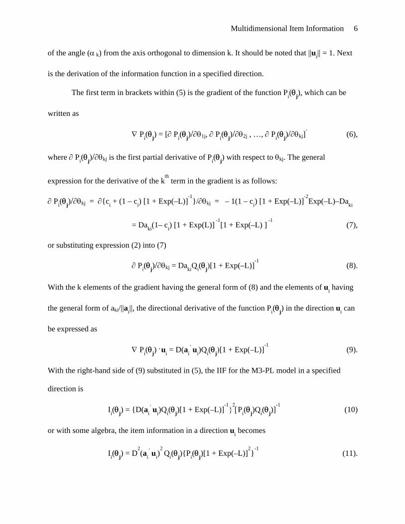
of the angle (α k) from the axis orthogonal to dimension k. It should be noted that ||ui|| = 1. Next

is the derivation of the information function in a specified direction.

The first term in brackets within (5) is the gradient of the function Pi(θj), which can be

written as

∇ Pi(θj) = [∂ Pi(θj)/∂θ1j, ∂ Pi(θj)/∂θ2j , …, ∂ Pi(θj)/∂θkj], (6),

where ∂ Pi(θj)/∂θkj is the first partial derivative of Pi(θj) with respect to θkj. The general

expression for the derivative of the kth

term in the gradient is as follows:

∂ Pi(θj)/∂θkj = ∂{ci + (1 – ci) [1 + Exp(–L)]-1

}/∂θkj = – 1(1 – ci) [1 + Exp(–L)]-2

Exp(–L)–Daki

= Daki(1– ci) [1 + Exp(L)] -1

[1 + Exp(–L) ] -1

(7),

or substituting expression (2) into (7)

∂ Pi(θj)/∂θkj = DakiQi(θj)[1 + Exp(–L)]-1

(8).

With the k elements of the gradient having the general form of (8) and the elements of ui having

the general form of aki/||ai||, the directional derivative of the function Pi(θj) in the direction ui can

be expressed as

∇ Pi(θj) · ui = D(ai

,ui)Qi(θj)[1 + Exp(–L)]

-1 (9).

With the right-hand side of (9) substituted in (5), the IIF for the M3-PL model in a specified

direction is

Ii(θj) = {D(ai

,ui)Qi(θj)[1 + Exp(–L)]

-1}

2[Pi(θj)Qi(θj)]

-1 (10)

or with some algebra, the item information in a direction ui becomes

Ii(θj) = D2(ai

,ui)

2 Qi(θj){Pi(θj)[1 + Exp(–L)]

2}

-1 (11).


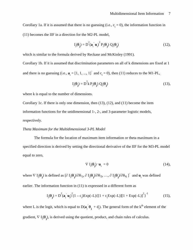
Corollary 1a. If it is assumed that there is no guessing (i.e., ci = 0), the information function in

(11) becomes the IIF in a direction for the M2-PL model,

Ii(θj) = D2(ai

,ui)

2 Pi(θj) Qi(θj) (12),

which is similar to the formula derived by Reckase and McKinley (1991).

Corollary 1b. If it is assumed that discrimination parameters on all of k dimensions are fixed at 1

and there is no guessing (i.e., ai = [1, 1, ..., 1], and ci = 0), then (11) reduces to the M1-PL,

Ii(θj) = D2k

Pi(θj) Qi(θj) (13),

where k is equal to the number of dimensions.

Corollary 1c. If there is only one dimension, then (13), (12), and (11) become the item

information functions for the unidimensional 1-, 2-, and 3-parameter logistic models,

respectively.

Theta Maximum for the Multidimensional 3-PL Model

The formula for the location of maximum item information or theta maximum in a

specified direction is derived by setting the directional derivative of the IIF for the M3-PL model

equal to zero,

∇ Ii(θj) · ui = 0 (14),

where ∇ Ii(θj) is defined as [∂ Ii(θj)/∂θ1j, ∂ Ii(θj)/∂θ2j, …, ∂ Ii(θj)/∂θkj ],

and ui was defined

earlier. The information function in (11) is expressed in a different form as

Ii(θj) = D2(ai

,ui)

2(1 – ci)Exp(–L){[1 + ciExp(–L)][1 + Exp(–L)]

2}

-1 (15),

where L is the logit, which is equal to D(ai

,θj + di). The general form of the kth element of the

gradient, ∇ Ii(θj), is derived using the quotient, product, and chain rules of calculus.


∂ Ii(θj) / ∂θkj = ∂ D2(ai

,ui)

2(1 – ci)Exp(–L){[1 + ciExp(–L)][ 1 + Exp(–L)]

2}

-1 / ∂θkj

= [–Daki D2(ai

,ui)

2(1 – ci)Exp(–L) [1 + ciExp(–L)] [1 + Exp(–L)]

2 –

{2[1 + Exp(–L)] Exp(–L) – Daki[1+ ciExp(–L)] + [1 + Exp(–L)]2ciExp(–L)–Daki } D

2 (ai

,ui)

2(1–

ci)Exp(–L)]{[1 + ciExp(–L)][1 + Exp(–L)]2}

-2

= [–aki D3(ai

,ui)

2 [Exp(–L) – ciExp(–L)] [1 + ciExp(–L)] [1 + Exp(–L)]

2 +

aki2Exp(–L) [1 + Exp(–L)] [1+ ciExp(–L)] D3(ai

,ui)

2[Exp(–L) – ciExp(–L)] +

akiciExp(–L) [1 + Exp(–L)]2 D

3(ai

,ui)

2 [Exp(–L) – ciExp(–L)]]{[1 + ciExp(–L)][1 + Exp(–L)]

2}

-2

= [aki D3(ai

,ui)

2 [Exp(–L) – ciExp(–L)] [1 + Exp(–L)]

2{–1 – ciExp(–L) + ciExp(–L)}+

aki2Exp(–L) [1 + Exp(–L)] [1+ ciExp(–L)] D3(ai

,ui)

2[Exp(–L) – ciExp(–L)]] {[1 + ciExp(–L)][1

+ Exp(–L)]2}

-2

= [aki D3(ai

,ui)

2 [Exp(–L) – ciExp(–L)] [1 + Exp(–L)]

2{–1} + aki2Exp(–L) [1 + Exp(–L)]

[1+ ciExp(–L)] D3(ai

,ui)

2[Exp(–L) – ciExp(–L)]]{[1 + ciExp(–L)][1 + Exp(–L)]

2}

-2

= D3aki(ai

,ui)

2 [Exp(–L) – ciExp(–L)] [1 + Exp(–L)] [{–1}[1 + Exp(–L)] + 2Exp(–L)

[1+ ciExp(–L)] ]{[1 + ciExp(–L)][1 + Exp(–L)]2}

-2

= D3aki(ai

,ui)

2 [Exp(–L) – ciExp(–L)] [1 + Exp(–L)] [{–1}[1 + Exp(–L)] + 2Exp(–L)

[1 + ciExp(–L)] ]{ [1 + ciExp(–L)]2[1 + Exp(–L)]

4}

-1

= D3aki(ai

,ui)

2 [Exp(–L) – ciExp(–L)] [{–1}[1 + Exp(–L)] + 2Exp(–L)


[1 + ciExp(–L)] ]{[1 + ciExp(–L)]2[1 + Exp(–L)]

3}

-1

= – D3aki(ai

,ui)

2[Exp(–L) – ciExp(–L)] [1 + Exp(–L)]{[1 + ciExp(–L)]

2[1 + Exp(–L)]

3}

-1

+ D3aki(ai

,ui)

2 [Exp(–L) – ciExp(–L)] 2Exp(–L) [1 + ciExp(–L)]{[1 + ciExp(–L)]

2[1 + Exp(–

L)]3}

-1

= –D3aki(ai

,ui)

2 [Exp(–L) – ciExp(–L)]{[1 + ciExp(–L)]

2[1 + Exp(–L)]

2 }

-1 +

D3aki(ai

,ui)

2 [Exp(–L) – ciExp(–L)] 2Exp(–L){[1 + ciExp(–L)] [1 + Exp(–L)]

3}

-1 (16).

From (16), the kth

element of the gradient ∇ Ii(θj) can be expressed as

∂ Ii(θj) / ∂θkj = [D3aki(ai

,ui)

2 [Exp(–L) – ciExp(–L)]{[1 + ciExp(–L)] [1 + Exp(–L)]

2}

-1]

{–1[1 + ciExp(–L)] -1

+ 2Exp(–L)[1 + Exp(–L)]-1

} (17).

With the k elements of the gradient, ∇ Ii(θj), having the general form of (17) and the elements of

ui have the general form of aki/||ai||, the directional derivative of the IIF, Ii(θj), in the direction ui

is expressed as

∇ Ii(θj) · ui = [D3(ai

,ui)

3 [Exp(–L) – ciExp(–L)]{[1 + ciExp(–L)] [1 + Exp(–L)]

2}

-1]

{–1[1 + ciExp(–L)]-1

+ 2Exp(-L)[1 + Exp(–L)]-1

}= 0 (18).

From (18), item information is maximized when the following condition is satisfied:

–1[1 + ciExp(–L)]-1

+ 2Exp(-L)[1 + Exp(–L)]-1

= 0 (19),

or Pi(θj) = .5Exp(L) (20).

Expression (20) is a necessary condition for maximizing item information for the

unidimensional and multidimensional 1-, 2-, and 3-PL models. In the unidimensional 1-PL

model, information is maximized when Pi(θj) = Qi(θj) = .5. When Pi(θj) is equal to .5, then the


natural logarithm of the odds of getting the item correct is 0, i.e., ln[Pi(θj)/Qi(θj)] = 0, which

implies that L in (20) is 0 and Exp(L) = 1. This leaves the well-known condition for maximizing

information in the 1- and 2-PL cases, which is Pi(θj) = Qi(θj) = .5. For the 3-PL unidimensional

and multidimensional models, the right-hand side of (20) and the probability of a correct

response are not equal to .5 when information is maximized, but the equality is satisfied at a

different value, which is primarily a function of guessing. The expression in (20) can also be

written as

2Exp(–L) = [Pi(θj)]-1

(21).

The probability of a correct response can also be written as

Pi(θj) = [Exp(L) + ci][Exp(L) + 1] -1

(22).

With the right-hand side of (22) substituted into (21),

2Exp(–L) = [Exp(L) +1][Exp(L) + ci] -1

(23).

To solve for L, expression (23) is written as

2 + 2ciExp(–L) = Exp(L) +1 (24).

After multiplying both sides by Exp(L),

2Exp(L) + 2ci = Exp(2L) + Exp(L) (25),

which, after subtracting 2Exp(L) from both sides, is equivalent to

2ci = Exp(2L) – Exp(L) (26).

After multiplying both sides by 4, expression (26) becomes

8ci = 4 Exp(2L) – 4Exp(L) (27).

When 1 is added to both sides, then (27) becomes

8ci + 1 = 4 Exp(2L) – 4Exp(L) + 1 (28).


By way of the binomial theorem, the equality of (28) can be written as

8ci + 1 = [2 Exp(L) – 1]2 (29),

which after taking the square root of both sides becomes

(8ci + 1)1/2

= 2 Exp(L) – 1 (30).

Solving for L in (30) gives

L = ln{.5 [1 + (8ci + 1)1/2

]} (31),

which becomes

D(ai

,θj + di) = ln{.5 [1 + (8ci + 1)

1/2 ]} (32).

Now the objective is to solve for the vector θ that maximizes the information function of the M3-

PL model in the direction ui. To that end,

ai

,θ = ln{.5 [1 + (8ci + 1)

1/2 ]}D

-1 – di (33).

Because ui

,= ai

,/||ai||, both sides are divided by ||ai|| or MDISCi that results in

ui

,θ = ln{.5 [1 + (8ci + 1)

1/2 ]}(D||ai||)

-1 – di(||ai||)

-1 (34),

Now both sides are pre-multiplied by ui,

ui ui

,

θ = ui[ln{.5 [1 + (8ci + 1)1/2

]}(D||ai||)-1

– di(||ai||) -1] (35).

Because the associative law holds for multiplication of matrices, the left-hand side of (35) can be

written as (ui ui

,)θ. The product of (ui ui

,) is a k by k matrix, U, which has a few properties that

should be noted: 1. It is symmetric, thus U = U,, 2. The determinant of the matrix U is zero (0),

thus it is singular, 3. U2 = U

,U = UU = U, thus U is idempotent, 4. The main diagonal elements

of U are cos2α ki, thus the trace of U [i.e., tr(U)] is equal to one (1), and 5. The rank of an


idempotent matrix is equal to its trace, thus the rank of U is equal to 1. With U substituted for ui

ui

,

, expression (35) is written as

Uθ = ui[ln{.5 [1 + (8ci + 1)1/2

]}(D||ai||)-1

– di(||ai||) -1] (36).

Pre-multiply both sides by U yields

UUθ = Uui[ln{.5 [1 + (8ci + 1)1/2

]}(D||ai||)-1

– di(||ai||) -1] (37).

By the third property mentioned above for U, (37) can be written as

Uθ = Uui[ln{.5 [1 + (8ci + 1)1/2

]}(D||ai||)-1

– di(||ai||) -1] (38).

Expression (38) is written as

Uθ – Uui[ln{.5 [1 + (8ci + 1)1/2

]}(D||ai||)-1

– di(||ai||) -1] = 0 (39),

where 0 is the same size as ui or by the distributive law for matrices,

U{θ – ui[ln{.5 [1 + (8ci + 1)1/2

]}(D||ai||)-1

– di(||ai||) -1]} = 0 (40).

Solutions that satisfy (40) are when U is equal to a null matrix (O) or when

θ = ui[ln{.5 [1 + (8ci + 1)1/2

]}(D||ai||)-1

– di(||ai||) -1] (41).

Therefore, theta maximum in a specified direction for the M3-PL model is

θmax = ui[ln{.5 [1 + (8ci + 1)1/2

]}(D||ai||)-1

– di(||ai||) -1] (42)

or substituting (3) and (4) into (42)

θmax = ui[ln{.5 [1 + (8ci + 1)1/2

]}(D.MDISCi )-1

+ MDIFFi] (43).

Several corollaries follow from this result in (43).

Corollary 2a. The location on the kth

dimension where information is maximized is given by


θmax k = [ln{.5 [1 + (8ci + 1)1/2

]}(D.MDISCi )-1

+ MDIFFi] cos αki (44).

Corollary 2b. If it is assumed that there is no guessing, i.e., ci = 0, expression (43) reduces to

θmax = MDIFFi ui (45).

Expression (45) is the same as that implied by Reckase and McKinley (1991) for the location of

maximum item information for the multidimensional 2-PL model.

Corollary 2c. If it is assumed that there is only one dimension, then the expression in (43)

reduces to the well-known formula for theta maximum derived by Birnbaum (1968),

θmax = ln{.5 [1 + (8ci + 1)1/2

]}(Dai )-1

+ bi (46).

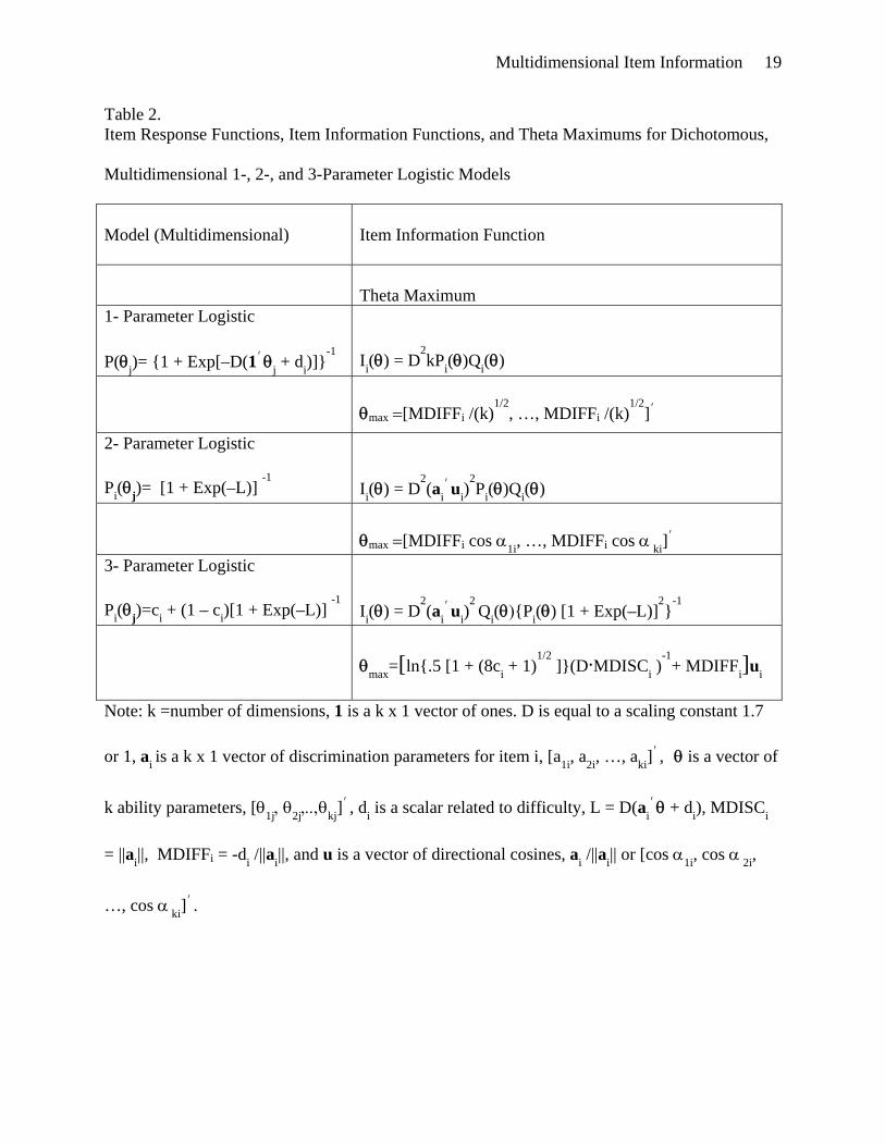
IIFs and formulas for location of maximum item information for the multidimensional 1-, 2-, and

3-PL models are listed in Table 2.

Derivations have been shown for the IIF and theta maximum in a specified direction. Now

an example item is given that uses the derived results. The following are hypothetical

parameters for the M3-PL model: ai = [a1i = 1.5, a2i = .5],, ci = .2, di = .5, and D =1.7. A

graphical illustration of the IIF is shown in Figure 1. It appears that this item gives more

information along the first dimension; this is supported by a higher discrimination parameter on

θ1 (1.5) relative to θ2 (.5). From expression (43), theta maximum is θmax = [-.206, -.069],. This is

verified by the condition satisfied by (20), i.e., Pi(θmax) = .5Exp[1.7(ai

,θmax + .5)] = .653. The

item can be considered as moderately easy with maximum information provided at θ1 = -.206

and θ2 = -.069. Multidimensional difficulty (MDIFFi) is -.316, which is lower than either element

in θmax. In the presence of guessing, this is consistent with values of theta maximum and


difficulty in the unidimensional case (Hambleton, et al, 1991). By (43) and (11), the maximum

amount of information in direction ui, [.949 .316],, at the location θmax is 1.23.

Conclusion

The purpose of this article was to present the IIF and theta maximum in a specific

direction for the M3-PL model. The M3-PL IIF was shown to be a general case of item

information for unidimensional 1-, 2-, and 3-PL models. A sufficient condition for maximizing

item information for unidimensional and multidimensional 1-, 2-, and 3-parameter logistic

models was given as Pi(θj) = .5Exp(L).

Researchers have shown that developing tests using the IIF is more efficient as compared

to other methods (Hambleton & de Gruijter, 1983; Hambleton, et al., 1991). Some evidence

suggests that using the location of maximum item information is the most effective for

unidimensional models (Gierl, Henderson, Jodoin, & Klinger, 2001). Future research may

explore the extent to which this generalizes to the multidimensional case. In research related to

computer-adaptive testing, algorithms for selecting items that fit the M3-PL model can be further

explored. Evidence suggests that item selection algorithms for computer-adaptive tests based on

multidimensional item response theory may be more effective than conventional unidimensional

IRT algorithms (Segall, 2001). In multidimensional adaptive testing (Segall, 1996), items are

selected to maximize some function of Fisher’s information matrix. For some testing purposes,

e.g., selection, this may be inefficient when decisions are made at a particular point (Samejima,

1977). Alternatively, the cut-off in a multidimensional, criterion-referenced test may be set at a

location given by [θ1, θ2, ..,θk]. Algorithms can select items that satisfy (20) and then compute

the value of information in the direction corresponding to the cut-off. Thus, the IIF presented in

this study may be useful for tests of this type. It is the intent of this article to provide some tools


[(11), (20), and (43)] that will give a better understanding of the measurement process in

compensatory measurement models.


References

Birnbaum, A. (1968). Some latent trait models and their use in inferring an examinee's ability. In

F.M. Lord and M.R. Novick, Statistical Theories of Mental Test Scores. Reading, MA:

Addison-Wesley.

Chang, H., Qian, J., & Ying, Z. (2001). a-stratified multistage computerized adaptive testing with

b blocking. Applied Psychological Measurement, 25(4), 333-341.

Embretson, S. E., & Reise, S. P. (2000). Item response theory for psychologists. Manwah, NJ:

Lawrence Erlbaum Associates.

Gierl, M.J., Henderson, D., Jodoin, M., & Klinger, D. (2001). Minimizing the influence of item

parameter estimation errors in test development: A comparison of three selection

procedures. The Journal of Experimental Education, 69(3), 261-279

Hambleton, R. K., & de Gruiter, D. N. (1983). Application of item response models to criterion-

referenced test item selection. Journal of Educational Measurement. 20(4), 355-367

Hambleton, R.K., Swaminathan, H. & Rogers, H.J. (1991). Fundamentals of Item Response

Theory. Newbury Park CA: Sage.

Lord, F.M. (1980). Application of Item Response Theory to Practical Testing Problems.

Hillsdale, NJ: Lawrence Erlbaum Associates.

Lord, F.M., & Novick, M. (1968). Statistical Theories of Mental Test Scores. Reading, MA:

Addison-Wesley.

Reckase, M. D. (1985). The difficulty of test items that measure more than one ability. Applied

Psychological Measurement, 9(4), 401-412.


Reckase, M. D., & McKinley, R. L. (1991). The discriminating power of items that measure

more than one dimension. Applied Psychological Measurement, 15(4), 361-373.

Reckase, M. D. (1997). A linear logistic multidimensional model for dichotomous item response

data. In W. J. van der Linden & R. K. Hambleton (Eds.), Handbook of modern item

response theory (pp. 271–286). New York: Springer-Verlag.

Samejima, F. (1977). A use of the information function in tailored testing. Applied Psychological

Measurement, 1, 233-247.

Segall, D. O. (1996). Multidimensional adaptive testing. Psychometrika, 61(2), 331-354.

Segall, D. O. (2001). General ability measurement: An application of multidimensional item

response theory. Psychometrika, 66(1), 79-97.

Weiss, D. J. (1982). Improving measurement quality and efficiency with adaptive testing.

Applied Psychological Measurement, 6, 473-492.


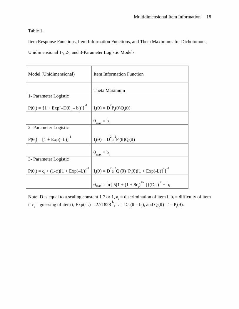
Table 1.

Item Response Functions, Item Information Functions, and Theta Maximums for Dichotomous,

Unidimensional 1-, 2-, and 3-Parameter Logistic Models

Model (Unidimensional)


Theta Maximum

1- Parameter Logistic P(θj) = {1 + Exp[–D(θj – bi)]}

-1

Ii(θ) = D

2Pi(θ)Qi(θ)

θmax = bi

2- Parameter Logistic P(θj) = [1 + Exp(–L)]

-1

Ii(θ) = D

2ai

2Pi(θ)Qi(θ)

θmax = bi

3- Parameter Logistic P(θj) = ci + (1-ci)[1 + Exp(–L)]

-1

Ii(θ) = D

2ai

2Qi(θ){Pi(θ)[1 + Exp(-L)]

2}

-1

θmax = ln{.5[1 + (1 + 8ci)

1/2 ]}(Dai)

-1 + bi

Note: D is equal to a scaling constant 1.7 or 1, ai = discrimination of item i, bi = difficulty of item

i, ci = guessing of item i, Exp(-L) = 2.71828-L

, L = Dai(θ – bi), and Qi(θ)= 1– Pi(θ).


Table 2. Item Response Functions, Item Information Functions, and Theta Maximums for Dichotomous,

Multidimensional 1-, 2-, and 3-Parameter Logistic Models

Model (Multidimensional)


Theta Maximum

1- Parameter Logistic P(θj)= {1 + Exp[–D(1

,θj + di)]}

-1

Ii(θ) = D

2kPi(θ)Qi(θ)

θmax =[MDIFFi /(k)

1/2, …, MDIFFi /(k)

1/2],

2- Parameter Logistic Pi(θj)= [1 + Exp(–L)]

-1

Ii(θ) = D

2(ai

,ui)

2Pi(θ)Qi(θ)

θmax =[MDIFFi cos α1i, …, MDIFFi cos α ki]

,

3- Parameter Logistic Pi(θj)=ci + (1 – ci)[1 + Exp(–L)]

-1

Ii(θ) = D

2(ai

,ui)

2 Qi(θ){Pi(θ) [1 + Exp(–L)]

2}

-1

θmax=[ln{.5 [1 + (8ci + 1)1/2

]}(D.MDISCi )-1

+ MDIFFi]ui

Note: k =number of dimensions, 1 is a k x 1 vector of ones. D is equal to a scaling constant 1.7

or 1, ai is a k x 1 vector of discrimination parameters for item i, [a1i, a2i, …, aki],, θ is a vector of

k ability parameters, [θ1j, θ2j,..,θkj],, di is a scalar related to difficulty, L = D(ai

,θ + di), MDISCi

= ||ai||, MDIFFi = -di /||ai||, and u is a vector of directional cosines, ai /||ai|| or [cos α1i, cos α 2i,

…, cos α ki],.


Figure Captions

Figure 1. Item Information Function for the 3-Parameter Logistic Multidimensional Model

Directional Item Information for the Multidimensional Three-Parameter Logistic Model

Documents

Transcript of Directional Item Information for the Multidimensional Three-Parameter Logistic Model