Direct controller order reduction by

identification in closed loop

Ioan Dore Landau a, Alireza Karimi b, Aurelian Constantinescu c

aLaboratoire d’Automatique de Grenoble,ENSIEG, BP 4638402 Saint Martin d’Heres, France

bSharif University of Technology, Electrical Engineering Dept.,Tehran 11365-9363, IRAN

cLaboratoire d’Automatique de Grenoble,ENSIEG, BP 4638402 Saint Martin d’Heres, France

Abstract

The paper 1 addresses the problem of directly estimating the parameters of a re-duced order digital controller using a closed loop type identification algorithm. Thealgorithm minimizes the closed loop plant input error between the nominal closedloop system and the closed loop system using the reduced order controller. It isassumed that a plant model (if necessary validated in closed loop with the nominalcontroller) is available. One of the original features of this approach is that it can useeither simulated or real data. The frequency bias distribution of the parameter esti-mates shows that the reduced order controller maintains the critical performance ofthe nominal closed loop system. A theoretical analysis is provided. Validation testsare proposed. Experimental results, obtained on an active suspension, illustrate theperformance of the proposed algorithms.

Key words: Controller reduction, closed loop identification, active suspension.

1 A preliminary version of this paper has been presented to the IFAC-SYSID Sym-posium, June 2000, S. Barbara, USA� Corresponding author I. D. Landau. Fax 33(0)4.76.82.63.88.E-mail landau@lag.ensieg.inpg.fr Tel. 33(0)4.76.82.63.91.��Alireza Karimi is currently with the Automatic Institute of Swiss Federal Instituteof Technology at Lausanne (EPFL).

Email addresses: alireza.karimi@epfl.ch (Alireza Karimi),aurelian@lag.ensieg.inpg.fr (Aurelian Constantinescu).

Preprint submitted to Elsevier Science 17 April 2001

� �

���� ����

�

����

� �

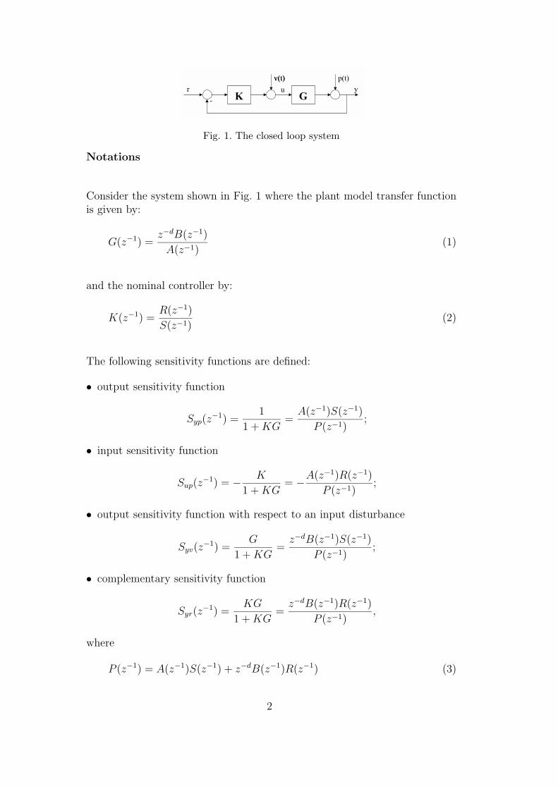
Fig. 1. The closed loop system

Notations

Consider the system shown in Fig. 1 where the plant model transfer functionis given by:

G(z−1) =z−dB(z−1)

A(z−1)(1)

and the nominal controller by:

K(z−1) =R(z−1)

S(z−1)(2)

The following sensitivity functions are defined:

• output sensitivity function

Syp(z−1) =

1

1 +KG=A(z−1)S(z−1)

P (z−1);

• input sensitivity function

Sup(z−1) = − K

1 +KG= −A(z−1)R(z−1)

P (z−1);

• output sensitivity function with respect to an input disturbance

Syv(z−1) =

G

1 +KG=z−dB(z−1)S(z−1)

P (z−1);

• complementary sensitivity function

Syr(z−1) =

KG

1 +KG=z−dB(z−1)R(z−1)

P (z−1),

where

P (z−1) = A(z−1)S(z−1) + z−dB(z−1)R(z−1) (3)

2

The system of Fig.1 will be denoted the “true closed loop system”. Throughoutthe paper we will consider feedback systems which will use either an estima-tion of G (denoted G) or a reduced order estimation of K (denoted K). Thecorresponding sensitivity functions will be denoted as follows:

• Sxy - Sensitivity function of the true closed loop system (K, G).

• Sxy - Sensitivity function of the nominal simulated closed loop system (nom-

inal controller K + estimated plant model G).

• ˆSxy - Sensitivity function of the simulated closed loop system using a re-

duced order controller (reduced controller K + estimated plant model G).

Similar notations are used for P (z−1): P (z−1) when using K and G,ˆP (z−1)

when using K and G.

1 Introduction

Controller design frequently results in high order controllers. On one hand thismay be the consequence of the complexity of the model used for design, onthe other hand robust controller design often results in complex high ordercontrollers even if the design model is of reasonable size. See for exampleLandau et al. (1995).

Controller reduction is a very important issue in many control applications ei-ther because the size of the controller is limited by hardware and computationtime or because simpler controllers are easier to implement and to under-stand. There are a number of approaches and methods for obtaining reducedorder controllers. See for example Zhou and Doyle (1998); Anderson (1993);Anderson and Liu (1989).

What is most important is to remember that controller reduction should aimto preserve the required closed loop properties as far as possible. Direct sim-plification of the controller using standard techniques (pole-zero cancellationwithin a certain radius, balanced reduction) without taking into account theclosed loop behaviour generally yields unsatisfactory results.

There are basically two approaches for controller reduction:

(1) Indirect approach:• Obtain a reduced order model which will capture the essential character-

istics of the nominal model in the critical frequency regions for design.• Design a new controller using the new low-order model.

(2) Direct approach:

3

�

��

������

��

�

�

�� �

�

��� ������������������������

�����������������������

���

�

�

�

�

�

�

��

Fig. 2. Closed loop identification of reduced order controllers using simulated data(input matching)

• Obtain an approximate reduced order controller which will preserve thenominal closed loop properties.

The indirect approach is subject to a number of criticisms. First of all, useof a reduced order model does not necessarily guarantee that the resultingcontroller will be of a sufficiently low order (design specifications usually be-come more complex when using model approximation). Secondly, the errorscaused by model approximation will spread to the subsequent design steps,see Anderson and Liu (1989); Cordons et al. (1999).

The direct approach to controller reduction seems more appropriate becausethe approximation is carried out in the final step of controller design and theresults can be easily understood. It should be noted that the controller result-ing from an indirect reduction procedure can be further reduced, if necessary,by application in the last step of a direct reduction approach.

Identification in closed loop offers an efficient methodology both for model or-der reduction and direct controller order reduction (see Bendotti et al. (1998)).

In this paper we will focus on the use of closed loop identification techniques fordirect controller order reduction. One of the basic block diagrams for reducedorder controller identification is shown in Fig. 2 (input matching scheme ). Theupper part represents the simulated nominal closed loop system. It is madeup of the nominal designed controller (denoted by K) and the best identifiedplant model (i.e which results in the closest behaviour of the true closed loopsystem and of the nominal simulated one and denoted by G).

The lower part is made up of the estimated reduced order controller (denoted

4

by K) in feedback connection with the plant model used for simulation ofthe nominal system. The parametric adaptation algorithm will try to find thebest reduced order controller of a given order which will minimize the closedloop input error expressed as the difference between the input to the plantmodel generated in the nominal simulated closed loop and the input to theplant model generated by the closed loop using the reduced order controller(i.e which will minimize the discrepancy between the two closed loops).

However, another objective for controller order reduction can be to minimizethe closed loop error between the plant output generated in the nominal sim-ulated closed loop and the plant output generated by the closed loop usingthe reduced order controller. As will be shown, this is possible using either thescheme of Fig. 2 but filtering the external excitation r through G or by addingthe external excitation to the input of the plant instead of to the input of thecontroller (in both cases the closed loop error, in the absence of disturbances,will reflect the difference between the two plant model outputs).

Identification of a reduced order controller is also possible using real dataas shown in Fig. 3 (the upper part represents the true closed loop system ).Note that the adjustable closed loop predictor (lower part) may use a plantmodel identified in closed loop with the nominal controller or more preciselythe plant model available which yields the best results when a “closed loop”model validation test is used (see Landau and Karimi (1997a); Landau et al.(1997)). In short, this plant model will minimize the discrepancy between thenominal true closed loop system and the simulated closed loop system usingthe nominal controller.

The method for direct controller reduction using real data may be related toiterative feedback tuning (IFT) in Hjalmarsson et al. (1998, 1994). The maindifferences are:(1)the IFT requires several experiments;(2) the IFT does notuse an estimated model of the plant to tune a reduced order controller.

The paper is organized as follows. In Section 2 some basic relationships con-sidered in controller reduction will be reviewed. In Section 3 the recursivealgorithms for direct identification of the reduced order controllers will bepresented and analyzed . Validation of the estimated reduced order controllerwill be discussed in Section 4. The practical aspects of the methodology will besummarized in Section 5. Experimental results concerning the identificationof reduced order controllers for active suspension will be given in Section 6.Finally we will have some concluding remarks.

5

�

�

������

��

�

�

�� �

�

��� ����������� ����

�������� ���� ���� �� �

���

�

�

�

�

�

�

��

�

��

�

��

�����

Fig. 3. Closed loop identification of the reduced order controllers using real data(input matching)

2 Direct Controller Reduction - Some basic facts

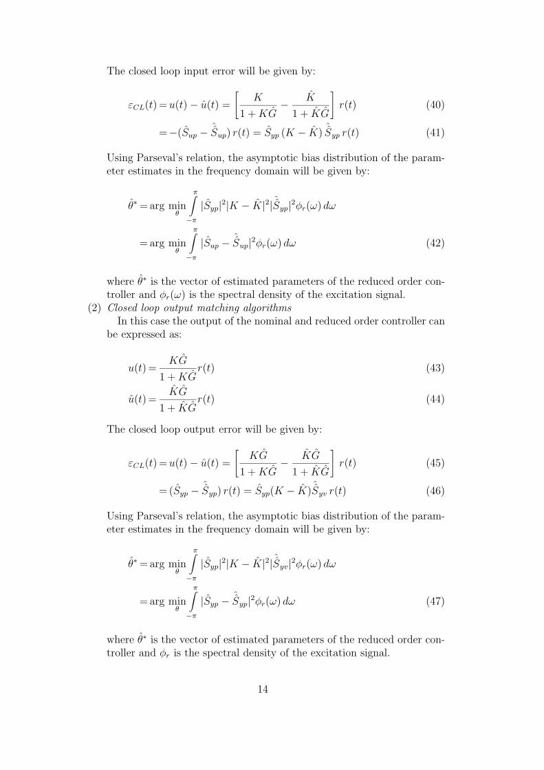
Several criteria for controller reduction have been proposed by Anderson (1993);Zhou and Doyle (1998). Their objective is the minimization of the discrep-ancy between the nominal closed loop and the loop using the reduced ordercontroller. Let us consider the block diagram of Fig. 2. Consider the “inputmatching” objective which aims to preserve performance with respect to theeffect of the output disturbance upon the plant input by minimization of theclosed loop error between the two plant inputs u and u. This is equivalent tominimizing the following norm:

‖Sup − ˆSup‖ =

∥∥∥∥∥ K

1 +KG− K

1 + KG

∥∥∥∥∥ (4)

where Sup is the input sensitivity function of the nominal simulated closed

loop andˆSup is the input sensitivity function when using the reduced order

controller. Therefore the optimal reduced order controller will be given by:

K∗ = arg minK

‖Sup − ˆSup‖ = arg min

K‖Syp(K − K)

ˆSyp‖ (5)

If we now consider preservation of performance in tracking, the reduced ordercontroller should minimize the following norm:

‖Syr − ˆSyr‖ =

∥∥∥∥∥ KG

1 +KG− KG

1 + KG

∥∥∥∥∥ (6)

6

In the same way as when preserving performance for output disturbance re-jection, the reduced order controller should minimize:

‖Syp − ˆSyp‖ =

∥∥∥∥∥ 1

1 +KG− 1

1 + KG

∥∥∥∥∥ (7)

Fortunately, these two norms are equal and the reduced order controller canbe obtained by the following expression:

K∗ = arg minK

‖Syp − ˆSyp‖ = arg min

K‖Syp(K − K)

ˆSyv‖ (8)

Eqs. (5) and (8) show that a weighted norm of K − K should be minimized.Several methods for solving this problem have been proposed in the literature.The model reduction using weighted balanced realization in Enns (1984) solvesan approximation of the problem, i.e. it neither minimizes the infinity normof the weighted error nor gives the error bounds. Another approach proposedby Anderson (1986) minimizes the Hankel norm of the weighted error as wellas giving the error bounds.

In this paper we present an approach for minimization of the 2-norms con-sidered in (5) and (8) by direct identification of a reduced controller in closedloop. The identification algorithm will minimize a 2-norm of a closed loop pre-diction error. We will show that the modeling error between the nominal andreduced order controller is exactly weighted with the filters of Eq. (5) or (8).Unstable parts and fixed parts of the controller, which should be preservedin the reduced order controller, can be easily treated. It is assumed that astabilizing controller of a given complexity exists and that the algorithm willsearch the parameters of this controller. Once such a reduced order controlleris obtained, it should be validated and validation tests are proposed. The Vin-nicombe distance between the two closed loop transfer functions (the nominalclosed loop and the closed loop using the reduced order controller) providesuseful information on the quality of the approximation. What is certainly veryinteresting and introduces new features for the proposed procedure is that ourpresentation shows that the reduced order controller can be identified usingreal data.

3 Algorithms for direct closed loop identification of reduced ordercontrollers

The parametric adaptation algorithms which will be used to identify the pa-rameters of a reduced order controller are very similar to the “closed loop out-

7

put error” (CLOE) algorithms used for plant model identification in closedloop. To a large extent, the problem of identification of reduced order con-trollers can be considered to be the dual of the reduced order plant modelidentification in closed loop (Landau and Karimi (1997a,b); Landau et al.(1997); Landau and Karimi (2000)). We will often refer to Landau and Karimi(1997a,b); Landau et al. (1997) for details of the algorithms and proofs.

3.1 Algorithms

Consider the upper part of Fig. 2. The nominal simulated closed loop is formedby the estimated plant model and the nominal controller. The estimated plantmodel is defined by the transfer operator (q−1 - unit delay operator):

G(q−1) =q−dB(q−1)

A(q−1)(9)

where:

B(q−1) = b1q−1 + · · · + bnB

q−nB = q−1B∗(q−1) (10)

A(q−1) = 1 + a1q−1 + · · · + anA

q−nA = 1 + q−1A∗(q−1). (11)

The plant model is operated in closed loop with a digital controller:

K =R(q−1)

S(q−1)(12)

where:

R(q−1) = r0 + r1q−1 + . . .+ rnR

q−nR (13)

S(q−1) = 1 + s1q−1 + . . .+ snsq

−nS = 1 + q−1S∗(q−1) (14)

u(t) is the plant input, y(t) is the plant output and r(t) is the external exci-tation signal (filtered if necessary).

The output of the nominal controller is given by:

u(t+ 1) = −S∗(q−1)u(t) +R(q−1)c(t+ 1) = θTψ(t) (15)

where

8

c(t+ 1) = r(t+ 1) − y(t+ 1) (16)

y(t+ 1) =−A∗y(t) + B∗u(t− d) (17)

ψT (t) = [−u(t), . . . ,−u(t− nS + 1), c(t+ 1), . . . , c(t− nR + 1)] (18)

θT = [s1, . . . , snS, r0, . . . , rnR

] (19)

To implement and analyze the algorithm, we need respectively the a priori(based on θ(t)) and the a posteriori (based on θ(t + 1)) predicted outputs ofthe estimated reduced order controller (of orders nS and nR) which are givenby (see the lower part of Fig. 2):

a priori:

u0(t+ 1) = u(t+ 1|θ(t)) = −S∗(t, q−1) u(t) + R(t, q−1) c(t+ 1)

= θT (t)φ(t) (20)

a posteriori:

u(t+ 1) = θT (t+ 1)φ(t) (21)

where:

θT (t) = [s1(t), . . . , snS(t), r0(t), . . . , rnR

(t)] (22)

φT (t) = [−u(t), . . . ,−u(t− nS + 1), c(t+ 1), . . . , c(t− nR + 1)] (23)

c(t+ 1) = r(t+ 1) − y(t+ 1) = r(t+ 1) + A∗y(t) − B∗u(t− d) (24)

3.1.1 Closed loop input matching algorithm (CLIM)

The closed loop input error is given by:

a priori:

ε0CL(t+ 1) = u(t+ 1) − u0(t+ 1) (25)

a posteriori:

εCL(t+ 1) = u(t+ 1) − u(t+ 1) (26)

and the parameter adaptation algorithm will be given by:

9

θ(t+ 1) = θ(t) + F (t)Φ(t)εCL(t+ 1) (27)

F−1(t+ 1) = λ1(t)F−1(t) + λ2(t)Φ(t)ΦT (t) (28)

0 < λ1(t) ≤ 1; 0 ≤ λ2(t) < 2; F (0) > 0

εCL(t+ 1) =ε0CL(t+ 1)

1 + ΦT (t)F (t)Φ(t)=u(t+ 1) − u0(t+ 1)

1 + ΦT (t)F (t)Φ(t)(29)

As we can see from (29), the a posteriori closed loop input error εCL(t + 1)can be expressed in terms of the a priori (measurable) closed loop input errorε0CL(t+1). Therefore the right hand side of (27) will depend only on measurablequantities at t+ 1. For more details see Landau et al. (1997).

Specific algorithms will be obtained by an appropriate choice of observationvector Φ(t) as follows:

• CLIM: Φ(t) = φ(t)

• F-CLIM: Φ(t) = A(q−1)

P (q−1)φ(t)

where:

P (q−1) = A(q−1)S(q−1) + q−dB(q−1)R(q−1). (30)

3.1.2 Closed loop output matching algorithm (CLOM)

The objective is to create a closed loop error which reflects the differencebetween the output y(t) of the nominal closed loop simulated system andthe output y(t) of the simulated closed loop system using the reduced ordercontroller. Two solutions are proposed:

(1) Filtering the external excitation (CLOM1)Consider the upper part of the Fig. 2. The output of the plant model

in the absence of disturbances is given by:

y(t) =KG

1 +KGr(t) (31)

Now, if instead of directly using r(t) we apply to the system r(t) filteredthrough G we obtain (see Fig. 4a):

u(t) =KG

1 +KGr(t) (32)

and therefore, in the absence of disturbances, the two transfer operatorsare the same. The situation is similar for the feedback system using thelower order controller K. Therefore, if we use the CLIM algorithms butfilter first r(t) by G, the algorithm will minimize the closed loop outputerror instead of the closed loop input error.

10

�

��

������

��

U

� \X

FÅ XÅ

FRQWUROOHU

RUGHUUHGXFHG

&/�

�

�

�

�

�

�

��

��

�

���U

[ X

[Å XÅ

�

�

�

�

�

�

��

������

&/�

��

FRQWUROOHURUGHUUHGXFHG

ORRS�FORVHGVLPXODWHGQRPLQDO

Fig. 4. Closed loop output matching (CLOM): a) CLIM algorithm with filteredexternal excitation (CLOM1); b) CLIM algorithm with external excitation appliedto the plant input (CLOM2)

(2) Adding the external excitation to the plant input (CLOM2)This is illustrated in Fig. 4b. By changing the point of application of

the external excitation, the relation between r(t) and u(t) is given by (32),i.e. in the absence of disturbances, the new u(t) will be equal to y(t). Foreffective implementation of the algorithm, the only changes occur in Eqs.(15) and (18) where c(t) is replaced by:

x(t) = G(r(t) − u(t)) (33)

Note also that for real time experiments (as well as in simulation), theorder of the blocks in the upper part of the scheme given in Fig. 4b canbe interchanged.

3.1.3 Imposing constraints on the reduced order controllers

Without difficulty, fixed parts (filters) can be forced in the reduced ordercontrollers (like integrators, opening of the loop at 0.5fs, fixed filters etc.).

11

For this, the nominal controller is factorized as K = KFK′ and the reduced

order controller is factorized as K = KF K′ where KF corresponds to the fixed

part of the controller that we would like to be contained in the reduced ordercontroller . Then a new input to the controller K ′ will be defined as c′ = KF cand c is replaced by c′ in the observation vector Φ .

3.2 Stability analysis

Using the results of the analysis given in Landau and Karimi (1997a,b); Lan-dau et al. (1997) and by duality arguments (interchanging B and A with Rand S respectively), it can be shown that if the estimated controller has thesame structure as the nominal controller, then the closed loop error goes tozero and the signals remain bounded, provided that a sufficient strict passivitycondition of the form

H ′(z−1) = H(z−1) − λ2; max

tλ2(t) ≤ λ < 2 (34)

is a strictly positive real transfer function is satisfied, where:

H =

A/P for CLIM

1 for F − CLIM(35)

Strictly positive real condition also requires that for CLIM (as well as for F-CLIM) A be an asymptotically stable polynomial. Note that for F-CLIM thepassivity condition is always satisfied since the filters which have to be usedin the algorithm contain known quantities. The same passivity conditions arevalid for the CLOM algorithm.

The passivity conditions (34) and (35) also guarantee the asymptotic unbi-asedness of the estimates in the presence of measurement noise (noise andexternal excitation are assumed to be independent).

In the case of estimation of a reduced order controller, the following assump-tions are made:

• There is a reduced order controller characterized by unknown polynomialsS (of order nS) and R (of order nR) which stabilizes the closed loop system.

• r(t) is norm bounded.• The output of the nominal controller (15) can be expressed as:

u(t+ 1) = −S∗(q−1)u(t) + R(q−1) c(t+ 1) + η(t+ 1) (36)

12

where η(t) is a norm bounded signal.

Equation (36) can be interpreted as a decomposition of the nominal controllerinto two parallel blocks: one is the reduced order controller and the other is theneglected part generating η(t). The boundedness of η(t) requires the neglectedpart to be stable. The practical consequence of this assumption is that anyunstable parts of the nominal controller should remain in the reduced ordercontroller. This can be imposed, for example, as a fixed part in the reducedorder controller.

Based on the results of Landau and Karimi (1997b) (pg. 1505-1506) and as-suming that r(t) is norm bounded, we can show that all the signals are normbounded under the passivity conditions (34) and (35). Therefore, when the es-timated controller does not have the same structure as the nominal controller,the above conditions ensure the boundedness of the closed loop input errorand closed loop output error respectively. For more details see Landau andKarimi (1997a,b).

Under the above assumptions a stable closed loop system will be obtained ifthe data length is long enough to allow convergence to the stabilizing controller(if there is not enough data, recycling of the data is possible).

3.3 Bias analysis

In the case of controller order reduction, by definition the estimated reducedorder controller does not have the same structure as the nominal controller.Therefore an asymptotic bias will occur which can be characterized in thefrequency domain.

We will now examine the bias for the various algorithms when using simulatedand real time data.

3.3.1 Use of simulated data

(1) Closed loop input matching algorithmThe output of the nominal and reduced order controller can be ex-

pressed as:

u(t) =K

1 +KGr(t) (37)

u(t) =K

1 + KGr(t) (38)

(39)

13

The closed loop input error will be given by:

εCL(t) =u(t) − u(t) =

[K

1 +KG− K

1 + KG

]r(t) (40)

=−(Sup − ˆSup) r(t) = Syp (K − K)

ˆSyp r(t) (41)

Using Parseval’s relation, the asymptotic bias distribution of the param-eter estimates in the frequency domain will be given by:

θ∗ = arg minθ

π∫−π

|Syp|2|K − K|2| ˆSyp|2φr(ω) dω

= arg minθ

π∫−π

|Sup − ˆSup|2φr(ω) dω (42)

where θ∗ is the vector of estimated parameters of the reduced order con-troller and φr(ω) is the spectral density of the excitation signal.

(2) Closed loop output matching algorithmsIn this case the output of the nominal and reduced order controller can

be expressed as:

u(t) =KG

1 +KGr(t) (43)

u(t) =KG

1 + KGr(t) (44)

The closed loop output error will be given by:

εCL(t) =u(t) − u(t) =

[KG

1 +KG− KG

1 + KG

]r(t) (45)

= (Syp − ˆSyp) r(t) = Syp(K − K)

ˆSyv r(t) (46)

Using Parseval’s relation, the asymptotic bias distribution of the param-eter estimates in the frequency domain will be given by:

θ∗ = arg minθ

π∫−π

|Syp|2|K − K|2| ˆSyv|2φr(ω) dω

= arg minθ

π∫−π

|Syp − ˆSyp|2φr(ω) dω (47)

where θ∗ is the vector of estimated parameters of the reduced order con-troller and φr is the spectral density of the excitation signal.

14

Expressions (42) and (47) clearly show that:

• The two norm expression of either Eq. (5) for CLIM (the difference between

Sup andˆSup) or Eq. (8) for CLOM (the difference between Syp and

ˆSyp) are

minimized when r(t) is a white noise signal (since the spectral density of awhite noise is a constant).

• The frequency distribution of the bias is weighted by the spectrum of thesensitivity functions of the nominal simulated system and the spectrumof the estimated sensitivity functions (given by the plant model and theestimated reduced order controller).

• The difference between K and K is minimized in the critical frequencyregions for control where the modulus of the sensitivity functions is large.

• The frequency distribution of the bias can be tuned by the choice of r(t).

3.3.2 Use of real data

(1) Closed loop input matching algorithmThe same algorithm applies when real data are used (Fig. 3). In this

case the expression of the closed loop error will be given by:

εCL(t) =

[K

1 +KG− K

1 + KG

]r(t) +

1

1 +KGv′(t) (48)

=−(Sup − ˆSup)r(t) + Sypv

′(t) (49)

where

v′(t) = v(t) −Kp(t) (50)

In Eq. (50) v(t) and p(t) represent the input and output disturbances(noise) respectively. The asymptotic bias distribution of the parameterestimates in the frequency domain will be given by:

θ∗ = arg minθ

π∫−π

{|Sup − ˆSup|2 φr(ω) + |Syp|2 φv′(ω)} dω

= arg minθ

π∫−π

{|Syp(K − K)ˆSyp + Sup(G−G)

ˆSup|2 φr(ω)

+|Syv|2 φv′(ω)} dω (51)

(2) Closed loop output matching algorithmsFor CLOM1, the controller output of the nominal and reduced order

controller can be expressed as:

u(t) =KG

1 +KGr(t) +

1

1 +KGv′(t) (52)

15

u(t) =KG

1 + KGr(t) (53)

The closed loop output error will be given by:

εCL(t) =u(t) − u(t) =

[KG

1 +KG− KG

1 + KG

]r(t) +

1

1 +KGv′(t)(54)

=Syp(K − K)ˆSyv r(t) + Sup(G−G)

ˆSyrr(t) + Syp v

′(t) (55)

Using Parseval’s relation again, the asymptotic bias distribution will begiven by:

θ∗ = arg minθ

π∫−π

{|Syp(K − K)ˆSyv + Sup(G−G)

ˆSyr|2 φr(ω)

+|Syp|2 φv′(ω)} dω (56)

For CLOM2 the output of the nominal controller is given by Eq. (52) inwhich G is replaced by G. The output of the reduced order controller isgiven by Eq. (53). This will finally yields to:

θ∗ = arg minK(θ)

π∫−π

{|Syp − ˆ

Syp|2φr(ω) + |Syp|2φv′(ω)}dω

= arg minK(θ)

π∫−π

{| ˆSyp(GK − GK)Syp|2φr(ω) + |Syp|2φv′(ω)

}dω

= arg minK(θ)

π∫−π

{| ˆSup(G− G)Syp − ˆ

Syp (K − K)Syv|2φr(ω)

+|Syp|2φv′(ω)}dω (57)

Expressions (51), (56) and (57) show that:

• The noise does not affect the asymptotic bias distribution of the controllerparameters estimate.

• The feedback system using the reduced order controller approximates thereal closed loop system instead of the nominal simulated system for CLIMand CLOM2.

• The frequency distribution of the bias can be tuned by the choice of r(t).

Eq. (57) (as well as Eqs. (51) and (56)) shows that the real data allows to takeinto account (in the good direction) the modeling error which always existsbetween the plant model used for controller reduction and the true plantmodel. Consider that G − G is small in some frequency regions (normally at

low frequencies), therefore the termˆSup(G − G)Syp can be ignored and the

16

minimization of the integral leads to the weighted minimization of |K − K|at low frequencies. Now consider that |G| << 1 in some frequency regions(normally at high frequencies), therefore the second term can be ignored andthe minimization of the integral leads to the minimization of the magnitude

of the input sensitivity function | ˆSup| at the frequencies where the modeling

error G − G is large, thus improving the robustness. For an example whichillustrates this property see Karimi and Landau (2000).

4 Validation of the estimated reduced order controller

Once a reduced order controller has been estimated, it must be validatedbefore it is applied on the real system.

4.1 Simulated Data

In this case we assume that the nominal controller stabilizes both the realplant and the plant model used in the reduction procedure. In actual factcontroller reduction takes place with respect to the available plant model whichis assumed to correspond to the real plant model. Also any uncertainties weretaken into account when the nominal controller was designed (as in all model-based controller reduction techniques). The resulting reduced order controllershould stabilize the nominal model and yield sensitivity functions which areclose to nominal ones in the critical frequency regions for performance androbustness.

In many applications, the output sensitivity function and the input sensitivityfunction are important. Therefore, in addition to testing closed loop stabilitywhen using a reduced order controller, it is necessary to check the closeness ofthe nominal and reduced order sensitivity functions in the frequency domainsince they are relevant both for performance and robustness.

The Vinnicombe distance (ν-gap) between the sensitivity functions obtainedwith the nominal and the reduced order controller, proposed in Vinnicombe(1993), uses a single number to make a first evaluation and classification ofthe results for various reduced order controllers. Then, a visual comparison ofthe frequency characteristics of the various sensitivity functions will allow usto decide whether the results obtained are satisfactory.

Another important aspect is tolerance with respect to the uncertainties be-tween the true plant model and the nominal plant model used for design andcontroller reduction. If we assume that this robustness issue was taken into

17

account when the nominal controller was designed, we have to try to pre-serve this property for the case of the reduced order controller. Comparisonof the sensitivity functions already provides valuable information, but morecomplete results can be obtained using the Vinnicombe stability test in Vin-nicombe (1993); Zhou and Doyle (1998). A controller Ki which stabilizes theplant model G1 will also stabilize all the plant models G2 satisfying the con-dition

δν(G1, G2) ≤ b(Ki, G1) (58)

where δν(G1, G2) is the ν-gap between the two plant models and b(Ki, G1)is the generalized stability margin defined as (Vinnicombe (1993); Zhou andDoyle (1998)):

b(Ki, G1) =

‖T (Ki, G1)‖−1

∞ if (Ki, G1) is stable

0 otherwise(59)

where

T (Ki, G1) =

Syr Syv

−Sup Syp

(60)

and Sxy are computed for (Ki, G1).

Therefore, in order to preserve the robustness of the reduced order controllerwith respect to the plant model uncertainties, we must check that b(Ki, G1)is close to b(K,G1), where K is the nominal controller and Ki is a reducedorder controller.

4.2 Real time data

In this case there are two options. The first one is to validate the reducedorder controller obtained with real time data using the validation methods for“simulated data” (see above). The second option is to take advantage of theavailable real time data. We will focus on this issue below.

With reference to Fig. 3, the objective is to test to what extent the estimatedclosed loop with a reduced order controller is close to the real closed loopsystem formed by the plant and the nominal controller.

18

Basic information is provided by the variance of the residual closed loop error.Moreover, as long as the complexity of the two closed loop systems is not toodifferent, the values of the cross-correlations between the residual closed looperror and the output of estimated controller generated in closed loop with theplant model are good indicators. This is similar to the statistical tests usedin closed loop identification (see Landau and Karimi (1997b); Landau et al.(1997)).

The other alternative for validation using real data is to compute the Vin-nicombe gap between the identified transfer function of the true closed loopsystem (between r and u) which uses the nominal controller and the computedtransfer function of the closed loop formed by the reduced order controller andthe estimated plant model.

5 Practical aspects

The controller reduction problem can be approached in two ways. The firstis to assume that the plant model is given and that the nominal controllerhas been designed allowing for both performance specification and supposeduncertainty of the model. This is the basic situation considered in all classicalreduction techniques, which results in the context of this paper in performingreduction using simulated data.

However, if access to the real-system is possible and the nominal controllercan be implemented, then there are two possibilities:

• improve the quality of the model by identification in closed loop (see Landauand Karimi (1997b); Landau et al. (1997));

• use real-data for controller reduction.

Once a plant model has been selected, the procedure for controller reduction isapplied using real data or simulated data (with a preference for real data). Thereduction procedure can scan all the orders for the polynomials R and S belowthe nominal ones using a single set of data. Those offering good approximationof the closed loop behaviour are selected.

6 Identification of reduced order controllers - Experimental results

The procedure for obtaining reduced order controllers by identification inclosed loop will be illustrated for the case of control of an active suspension.The active suspension is shown in Fig. 5 and the corresponding block diagram

19

FRQWUROOHU

UHVLGXDO DFFHOHUDWLRQ

SULPDU\ DFFHOHUDWLRQ �GLVWXUEDQFH�

�

��

�

PDFKLQH

VXSSRUW

HODVWRPHUH FRQH

LQHUWLD FKDPEHU

SLVWRQ

PDLQ

FKDPEHU

KROH

PRWRU

DFWXDWRU

�SLVWRQ

SRVLWLRQ�

Fig. 5. The active suspension system

in Fig.6. The controller via the power amplifier will act on the piston in orderto reduce the residual acceleration.The frequency spectrum of the vibrationswhich have to be reduced is limited by an upper frequency lower than 200 Hz.The system is controlled by a PC via an I/O board. Sampling frequency is800 Hz.

The primary acceleration was generated using a shaker. Its input is a signalgiven by the computer. The primary path model, between the excitation of theshaker and the residual acceleration, has several vibration modes: the first isat 31.47Hz with a damping factor 0.093. The goal is to compute a controllerwhich minimizes the residual acceleration around the first vibration modeand to try to distribute the amplification of the disturbances over the highfrequency range.

The identified plant model, between piston position and the residual acceler-ation (the secondary path), has the following complexity: nB = 11, nA = 12,d = 2. The system contains a double differentiator. Fig. 7 illustrates the fre-quency characteristics of two models for the secondary path:

(1) The open loop identified model, used to design the nominal controller.This model was identified in open loop using a PRBS generated by a 9-bitshift register, with a clock frequency of fs/4 (data length is L = 2048samples).

(2) The closed loop identified model, used to identify the reduced order con-trollers. This model gives better results in terms of closed loop validationand was identified in closed loop using the F-CLOE method (see Lan-dau and Karimi (1997a)), the nominal controller and the same excitationsignal as in open loop identification.

The results for controller reduction are given for the model identified in closedloop. The model has six vibration modes. Five of the six vibration modes have

20

a very low damping (< 0.085). Note that an important attenuation on Syp isrequired at the frequency of the first vibration mode.

��

�

�������������

����� ����

� ��

����� ������������������

���������� �����

������ ��������� �����

Fig. 6. Block diagram of the active suspension system

The nominal controller was designed using the “pole placement with sensitiv-ity function shaping by convex optimization” method (see Langer and Landau(1999)). A pair of dominant poles was fixed at the frequency of the first vi-bration mode, with a damping ξ = 0.8. In addition, a fixed part HR = 1+ q−1

was introduced in the controller (R = HRR′) to ensure opening of the loop

at 0.5fs. The resulting nominal controller satisfying the residual accelerationspecifications was obtained. Its complexity is given by the orders of polyno-mial R and S: nR = 27, nS = 28. Note that if standard pole placement is used,by solving the Bezout equation, the result will be a controller with the orders:nR = 12, nS = 13 (considering the fixed part HR).

First, the CLIM direct identification method for a reduced order controller wasused, based on simulated data. The external input was a PRBS generated bya 10-bit shift register, with a clock frequency of fs/2 (data length is L = 4096samples). A variable forgetting factor with λ1 = 0.95 and λ0 = 0.9 was used(λ1(t) = λ0λ1(t− 1) + 1 − λ0).

0 50 100 150 200 250 300 350 400−40

−30

−20

−10

0

10

20

30

40Active suspension identified models (open and closed loop)

Mag

nitu

de [d

B]

f [Hz]

Open loop identified modelf1 = 31.98 Hz; xi = 0.078f2 = 145.08 Hz; xi = 0.712f3 = 158.59 Hz; xi = 0.040f4 = 239.56 Hz; xi = 0.037f5 = 279.19 Hz; xi = 0.028f6 = 364.73 Hz; xi = 0.016

Closed loop identified modelf1 = 32.76 Hz; xi = 0.085f2 = 107.70 Hz; xi = 0.641f3 = 157.13 Hz; xi = 0.062f4 = 221.92 Hz; xi = 0.024f5 = 273.02 Hz; xi = 0.033f6 = 371.13 Hz; xi = 0.045

Fig. 7. The frequency characteristics of the secondary path models (input: pistondisplacement, output: residual acceleration)

21

0 0.05 0.1 0.15 0.2 0.25 0.3 0.35 0.4 0.45 0.5−8

−6

−4

−2

0

2

4Syp − Output sensivity function

f / fs

dB

Nominal (nR = 27, nS = 28)nR = 19, nS = 20 nR = 12, nS = 13 nR = 9, nS = 10

Fig. 8. Output sensitivity for the active suspension (controller reduction using CLIMalgorithm on simulated data)

0 0.05 0.1 0.15 0.2 0.25 0.3 0.35 0.4 0.45 0.5−50

−40

−30

−20

−10

0

10

Sup − Input sensivity function

f / fs

dB

Nominal (nR = 27, nS = 28)nR = 19, nS = 20 nR = 12, nS = 13 nR = 9, nS = 10

Fig. 9. Input sensitivity for the active suspension (controller reduction using CLIMalgorithm on simulated data)

The frequency characteristics of the sensitivity functions (Syp, Sup) and of thevarious controllers for the nominal controller (Kn) with nR = 27, nS = 28,and for three reduced order controllers: K1 with nR = 19, nS = 20, K2 withnR = 12, nS = 13 and K3 with nR = 9, nS = 10 are shown in figures 8 and9 respectively (a fixed part HR = 1 + q−1 was imposed in the reduced ordercontrollers).

22

Kn K1 K2 K3

Controller nR = 27 nR = 19 nR = 12 nR = 9

nS = 28 nS = 20 nS = 13 nS = 10

1 δν(Kn, Ki) 0 0.1810 0.5049 0.5180

2 δν(Snup, S

iup) 0 0.1487 0.4388 0.4503

3 δν(Snyp, S

iyp) 0 0.0928 0.1206 0.1233

4 b(Ki, G) 0.0800 0.0786 0.0685 0.0810

5 δν(CL(Kn), CL(Ki)) 0.1296 0.2461 0.5435 0.5522

6 C.L. error variance 0.0023 0.0083 0.0399 0.0398Table 1Comparison of the various controllers (controller reduction using CLIM algorithmon simulated data)

Note that the reduced controller K2 corresponds to the complexity of the poleplacement controller with the fixed part HR, (i.e. as a side result, the approachproposed here seeks out an optimal configuration for the closed loop poles inorder to achieve the stipulated performance). Complexity of controller K3 islower than that corresponding to pole placement. It is also important to see thevalues of the various ν-gap. These results are summarized in the Table 1 (therows 1 to 3). The last 2 rows in Table 1 summarize real time results. We observethat the generalized stability margins b(Ki, G) computed with the nominalmodel for the various reduced order controllers are close to the stability marginobtained with the nominal controller. Row 5 gives the ν-gap between theinput/output transfer function corresponding to the input sensitivity functionSup of the true closed loop system formed by the nominal designed controllerwith the real plant (obtained by identification) and the input/output transfer

function of the simulated closed loop system (ˆSup) formed by the various

controllers (including the nominal one and the reduced ones obtained usingsimulated data) in feedback connection with the plant model. This quantityis denoted by δν(CL(Kn), CL(Ki)). This is a good criterion for validation ofthe reduced order controller. Row 6 gives the variance of the residual closedloop input error between the true system and the simulated one. We observethat the ν− gap and the closed loop error variance have a coherent evolution.

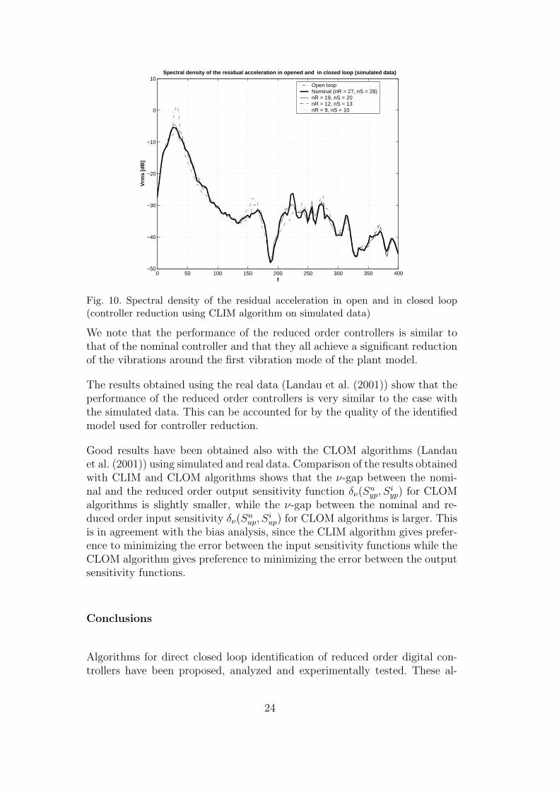
To illustrate the performance of the resulting controllers (Kn, K1, K2 andK3) on the real system, the spectral density of the residual acceleration inopen and in closed loop is shown in Fig. 10. The primary source of vibration(shaker’s excitation) is a PRBS. The characteristics obtained in closed loopoperation with the four controllers are compared with the characteristic of theopen loop operation (the interesting frequency range is 0 to 0.25fs (200 Hz)).

23

0 50 100 150 200 250 300 350 400−50

−40

−30

−20

−10

0

10

f

Spectral density of the residual acceleration in opened and in closed loop (simulated data)

Vrm

s [d

B]

Open loop Nominal (nR = 27, nS = 28)nR = 19, nS = 20 nR = 12, nS = 13 nR = 9, nS = 10

Fig. 10. Spectral density of the residual acceleration in open and in closed loop(controller reduction using CLIM algorithm on simulated data)

We note that the performance of the reduced order controllers is similar tothat of the nominal controller and that they all achieve a significant reductionof the vibrations around the first vibration mode of the plant model.

The results obtained using the real data (Landau et al. (2001)) show that theperformance of the reduced order controllers is very similar to the case withthe simulated data. This can be accounted for by the quality of the identifiedmodel used for controller reduction.

Good results have been obtained also with the CLOM algorithms (Landauet al. (2001)) using simulated and real data. Comparison of the results obtainedwith CLIM and CLOM algorithms shows that the ν-gap between the nomi-nal and the reduced order output sensitivity function δν(S

nyp, S

iyp) for CLOM

algorithms is slightly smaller, while the ν-gap between the nominal and re-duced order input sensitivity δν(S

nup, S

iup) for CLOM algorithms is larger. This

is in agreement with the bias analysis, since the CLIM algorithm gives prefer-ence to minimizing the error between the input sensitivity functions while theCLOM algorithm gives preference to minimizing the error between the outputsensitivity functions.

Conclusions

Algorithms for direct closed loop identification of reduced order digital con-trollers have been proposed, analyzed and experimentally tested. These al-

24

gorithms are the dual of closed loop output error identification algorithms.The algorithms try to minimize either the error between inputs generated inclosed loop operation by the nominal controller and the estimated reducedorder controller, or the closed loop output error between the two loops.

The possibility of using real data for estimation of reduced order controllersmakes it possible to take into account to a certain extent in the reductionprocedure, the discrepancies between the true plant and the plant model usedfor design and controller reduction.

While the specific algorithms proposed have a recursive form, it is also possibleto develop iterative algorithms along the lines used for closed loop identifica-tion (see Van Donkelaar and Van den Hof (2000)). Unfortunately this willraise similar theoretical problems.

Validation tests related to the ν−gap and Vinnicombe stability test have beenproposed. Use of the results given in Vinnicombe (1993, 1996); Anderson andGevers (1998) for reduced order controller validation deserve further investi-gation. Future work should consider the extension to the multivariable case.

Acknowledgements

The authors would like to thank one of the anonymous reviewers for his sug-gestions concerning the interpretation of the validation tests.

References

[1] Anderson, B., Gevers, M., 1998. Fundamental problems in adaptive control.In: Normand-Cyrot, D. (Ed.), Perspectives in Control. Springer-Verlag, Lon-don, UK.

[2] Anderson, B. D. O., 1986. Weighted Hankel norm approximation: Calculationof bounds. Systems and Control Letters 7 (4), 247–255.

[3] Anderson, B. D. O., August 1993. Controller design: Moving from theory topractice. IEEE Control Magazine .

[4] Anderson, B. D. O., Liu, Y., August 1989. Controller reduction: Concepts andapproaches. IEEE Transactions on Automatic Control 34 (8), 802–812.

[5] Bendotti, P., Cordons, B., Falinower, C., Gevers, M., December 1998. Controloriented low order modeling of a complex PWR plant: a comparison betweenopen loop and closed loop methods. In: IEEE-CDC 1998 (FAO 7-2). Tampa,Florida USA.

[6] Cordons, B., Bendotti, P., Falinower, C., Gevers, M., December 1999. A com-

25

parison between model reduction and controller reduction: Application toa PWR nuclear plant. In: IEEE-CDC. ix, USA, pp. 4625–4630.

[7] Enns, D., December 1984. Model reduction with balanced realization: An errorbound and a frequency weighted generalization. In: 23-rd CDC. Las Vegas,Nevada USA, pp. 127–132.

[8] Hjalmarsson, H., Gevers, M., Gunnarsson, S., Lequin, O., 1998. Iterative feed-back tuning: Theory and application. IEEE Control Systems Magazine ,26–41.

[9] Hjalmarsson, H., Gunnarsson, S., Gevers, M., December 1994. A convergentiterative restricted complexity control design scheme. In: 33rd IEEE-CDC.

[10] Karimi, A., Landau, I. D., June 2000. Controller order reduction by directclosed loop identification (output matching). In: 3rd Rocond IFAC. Prague.

[11] Landau, I. D., Karimi, A., May 1997a. An output error recursive algorithmfor unbiased identification in closed loop. Automatica 33 (5), 933–938.

[12] Landau, I. D., Karimi, A., August 1997b. Recursive algorithms for identifica-tion in closed loop - a unified approach and evaluation. Automatica 33 (8),1499–1523.

[13] Landau, I. D., Karimi, A., December 2000. Model estimation and controllerreduction: Dual closed loop identification problems. In: 39-th IEEE-CDC.Sydney.

[14] Landau, I. D., Karimi, A., Constantinescu, A., 2001. Direct controller orderreduction by identification in closed-loop - application to active suspensioncontrol. Tech. rep., Laboratoire d’Automatique de Grenoble, ENSIEG, BP.46, 38402 St. Martin d’Heres.

[15] Landau, I. D., Lozano, R., M’Saad, M., 1997. Adaptive Control. SpringerVerlag, London.

[16] Landau, I. D., Rey, D., Karimi, A., Voda, A., Franco, A., 1995. A flexibletransmission system as a benchmark for robust digital control. EuropeanJournal of Control 1 (2).

[17] Langer, J., Landau, I., 1999. Combined pole placement/sensitivity functionshaping method using convex optimization criteria. Automatica 35, 1111–1120.

[18] Van Donkelaar, E. T., Van den Hof, P. M. J., 2000. Analysis of closed-loopidentification with tailor-made parameterization. European Journal of Con-trol 6 (1), 54–62.

[19] Vinnicombe, G., 1993. Frequency domain uncertainty and the graph topology.IEEE Trans. on Automatic Control 38, 1571–1583.

[20] Vinnicombe, G., 1996. The robustness of feedback systems with bounded com-plexity. IEEE Trans. on Automatic Control 41 (6), 1571–1583.

[21] Zhou, K., Doyle, J. C., 1998. Essentials of robust control. Prentice-Hall, N.Y.

26