Transportation Research Part E 47 (2011) 532–546

Contents lists available at ScienceDirect

Transportation Research Part E

journal homepage: www.elsevier .com/locate / t re

Operational and environmental performance measuresin a multi-product closed-loop supply chain

Turan Paksoy a, Tolga Bektas� b,⇑, Eren Özceylan a

a Selçuk University, Department of Industrial Engineering, Campus, 42031 Konya, Turkeyb School of Management, University of Southampton, Highfield, Southampton SO17 1BJ, UK

a r t i c l e i n f o

Article history:Received 4 April 2010Received in revised form 30 September2010Accepted 4 December 2010

Keywords:Closed-loop chainsGreenhouse gas emissionsGreen supply chainMathematical modelling

1366-5545/$ - see front matter � 2010 Elsevier Ltddoi:10.1016/j.tre.2010.12.001

⇑ Corresponding author. Tel.: +44 (0)23 8059 896E-mail address: T.Bektas@soton.ac.uk (T. Bektas�)

a b s t r a c t

This paper investigates a number of operational and environmental performance measures,in particular those related to transportation operations, within a closed-loop supply chain.A mathematical model in the form of a linear programming formulation is used to modelthe problem, which captures the trade-offs between various costs, including those of emis-sions and of transporting commodities within the chain. Computational results are pre-sented for a number of scenarios, using a realistic network instance.

� 2010 Elsevier Ltd. All rights reserved.

1. Introduction

A supply chain refers to a broad set of activities associated with the transformation and flow of goods and services, includ-ing the flow of information, from the sources of materials to end-users (Bowersox and Closs, 1996). A typical supply chainprimarily consists of a number of production facilities serving a number of market regions, and the transportation of goodsfrom source to intermediate locations, and ultimately to end-users. Flow of material from source to end-users in a supplychain is via the so-called forward chain. Recent interest in supply chains lies in the recovery of products, which is typicallyachieved through processes such as repair, remanufacturing and recycling, which, combined with all the associated trans-portation and distribution operations, are collectively termed reverse chain activities. A supply chain in which forwardand reverse supply chain activities are integrated is said to be one of a closed-loop, and research on such chains have givenrise to the field of closed-loop supply chains (CLSCs).

One of the significant sources of greenhouse gas emissions and air pollution within a supply chain is transportation activ-ity, which has harmful effects on human health and undesirable consequences, such as global warming. Most of the researchdevoted to the design of supply chains has focused on operational performance metrics, such as cost of production, purchas-ing and transportation, profit, and tax (Meixell and Gargeya, 2005) and has neglected the environmental aspects. Given re-cent concerns on the harmful consequences of supply chain activities on the environment, and transportation in particular, ithas become necessary to specifically take into account environmental factors when planning and managing a supply chain.The list of environmental performance metrics of a supply chain is long, and includes emissions, energy use and recovery,spill and leak prevention and discharges (Hervani et al., 2005).

Green supply chain (GrSC) design extends the traditional definition of a supply chain by explicitly considering thefollowing factors in the design process: (i) waste resulting from any processes within the chain, (ii) energy efficiency, (iii)

. All rights reserved.

9; fax: +44 (0)23 8059 3844..

T. Paksoy et al. / Transportation Research Part E 47 (2011) 532–546 533

greenhouse gas emissions, and (iv) legal environmental requirements. Among the listed factors, greenhouse gas emissions,and CO2 in particular, are by far the most prominent with respect to their hazardous consequences on human health. Onesource of these emissions within a supply chain is the transportation activities that take place between various componentsin the chain.

In this study, we model and analyze a multi-product CLSC with an explicit focus on greenhouse gas emissions of the trans-portation activities, and the costs thereof, as well as product recovery. The model is in the form of a linear programming for-mulation and allows for the use of different modes of transport, each of which has its own emission rates and costs. Themodel also considers normal operational transportation costs, as well as various capacity limits on production and distribu-tion. The contributions of this paper to the literature are twofold: (i) we consider environmental costs within a closed-loopsupply chain network, mainly reflecting those of CO2 emissions due to transporting material in forward and reverse logisticsnetworks, and (ii) using the proposed model and a sample problem instance, we present results of computational experi-ments that shed light on the interactions of various performance indicators, primarily measured by cost, but also capturingthe environmental aspects.

The rest of the paper is organized as follows: Section 2 presents a brief review of the literature on GrSC and CLSC. In Sec-tion 3, we describe a mathematical model for the CLSC. Results of computational experiments, using a sample instance aregiven in Section 4. Main conclusions are offered in Section 5.

2. A brief review of the literature

This section presents a brief overview of the existing literature on GrSCs and CLSCs. There is a growing body of literatureon supply chain network design concerned with environmental issues, collectively named as GrSC. A comprehensive surveyof the field is provided by Srivastava (2007). We now provide a brief review of the literature that is relevant to the focus ofthe present paper.

Beamon (2008) describes the challenges and opportunities facing the supply chain of the future and describes sustainabil-ity and effects on supply chain design, management and integration. Traditional supply chains and GrSCs are compared andcontrasted, focusing on several important opportunities in GrSC management, including those in manufacturing, bio-waste,construction and packaging (Beamon, 1999).

Sarkis (2003) provides a strategic decision framework for green supply chain management, in which he investigates theuse of an analytical network process for making decisions within the GrSC. Sheu et al. (2005) present a multi-objective linearprogramming model for optimizing the operations of a green supply chain, composed of forward and reverse flows, includingdecisions pertaining to shipment and inventory. The model is based on a typical five-layer chain and considers a single prod-uct only, although it is applicable to any industry. The authors present computational results of the model based on the dataset of a notebook computer manufacturing chain. Ferretti et al. (2007) present a case-study based on an aluminum supplychain and an associated model to design a single buyer, single vendor green supply chain that minimizes the cost and pol-lution of production and distribution. The model is tested on a real supply chain in Lombardy, Italy, yielding an improvedchain design with reduced pollution levels.

Network chain members of a CLSC can be classified into two groups (Zhu et al., 2008): (1) Forward logistics chain mem-bers, including raw material suppliers, manufacturers, retailers and demand markets; and (2) Reverse logistics chain mem-bers, including demand markets, recovery centres and manufacturers. Manufacturers and demand nodes (i.e. customers)could be seen as ‘junction’ points where the forward and the reverse chains are combined to form the CLSC network. A recentoverview of the field from a business perspective is provided by Guide and Wassenhove (2009).

A number of papers appear in the literature focusing on the design of the reverse logistics network, or that of the closed-loop supply chain. We provide some pointers to the relevant literature. A closed-loop logistics model for remanufacturinghas been studied by Jayaraman et al. (1999) in which decisions relevant to shipment and remanufacturing of a set of prod-ucts, as well as establishment of facilities to store the remanufactured products are taken into consideration. The model is inthe form of a 0–1 integer programming formulation and minimizes a total cost function of shipment, remanufacturing andinventory. Fleischmann et al. (2001) consider a reverse logistics network design problem in which they analyze the impact ofproduct return flows on logistics networks. Guide et al. (2003) take a contingency approach in running CLSCs with productrecovery. The problem of consolidating returned products in a CLSC has been studied by Min et al. (2006) who propose amixed-integer, nonlinear programming model and a genetic algorithm for its solution. Kannan et al. (2010) developed a mul-ti echelon, multi period, multi-product CLSC network model for product returns, in which decisions are made regardingmaterial procurement, production, distribution, recycling and disposal. Yang et al. (2009) developed a model of a generalCLSC network, which includes raw material suppliers, manufacturers, retailers, customers and recovery centres. For an excel-lent review of methodological and case-study based papers in reverse and closed-loop logistics network design, the reader isreferred to Aras et al. (2010).

One of the first studies, to our knowledge, to consider environmental issues within CLSCs is by Krikke et al. (2001, 2003)who examine a supply chain design problem for refrigerators. The authors offer a comprehensive mathematical model thatnot only minimizes costs associated with distribution, processing and facility set-up, but also takes into account the envi-ronmental costs of energy and waste. Our study is similar to that of Krikke et al. in spirit, although we also consider multipleproducts in the supply chain network, restricting our attention to material flows rather than to decisions pertaining to

534 T. Paksoy et al. / Transportation Research Part E 47 (2011) 532–546

processing and facility set-up. In the next section, we present a formal definition of the problem studied in this paper, to-gether with an associated mathematical model.

3. Problem definition and modelling

In this paper, we consider a closed-loop supply chain in which the chain members are broadly classified into two groups:(i) forward chain entities, and (ii) reverse chain entities. The former is used to produce and deliver products to end-users,whereas the latter is used for recycling or waste-disposal of the same products. The network is structured as a typical 5-layerforward supply chain (Sheu et al., 2005), namely: (i) raw material supply, (ii) plants, (iii) warehouses, (iv) distribution cen-tres, (v) customers (end-users). Let S denote the index set of suppliers, Q denote the index set of plants, V denote the index ofwarehouse, K denote the index set of distribution centres (DCs), L denote the index set of customers. Similarly, a 5-layerstructure is considered for the reverse chain, including: (i) collection centres, (ii) repairing centres, (iii) dismantlers, (iv)decomposition centres, (v) final disposal locations of waste material. Let M denote the index set of collection centres, U de-note the index set of repairing centres, P denote the index set of dismantlers, O denote the index set of disposal and D denotethe index set of decomposition centres. Consider a supply chain network which consists of forward part Gf = (Nf, Af), whereNf = {S [ Q [ V [ K [ L} is the set of forward nodes and Af = {(i, j) | (i 2 S, j 2 Q) [ (i 2 Q, j 2 V) [ (i 2 Q, j 2 K) [ (i 2 V, j 2 K) [(i 2 V, j 2 L) [ (i 2 K, j 2 L)} is the set of ‘‘forward’’ arcs, and a reverse part Gr = (Nr, Ar), where Nr = M [ U [ P [ O [ D is theset of reverse nodes and Ar = {(i, j) | (i 2 L, j 2M) [ (i 2M, j 2 U) [ (i 2M, j 2 P) [ (i 2 P, j 2 O) [ (i 2 P, j 2 D)} is the set of reversearcs. The overall network on which the problem is modelled is denoted by G = (N, A) where N = Nf [ Nr and A = Af [ Ar [ {(i, j) |(i 2 U, j 2 K) [ (i 2 U, j 2 V) [ (i 2 D, j 2 S) [ (i 2 D, j 2 Q)} where the third set is the set of arcs linking the reverse chain back tomembers of the forward chain.

The network includes a number of suppliers (i.e. set S) that provide a number of different types of raw materials to plantsin which they are transformed into the same number of different products. We denote by R the index set of products. Eachproduct has an associated recycling rate, specifying the rate at which the product can be recycled. For instance, a rate of 100%indicates that the used product can be fully recovered or transformed into a new one, whereas a rate of 50% denotes that theproduct can only be partially recovered. An example of partial recovery is a PC, which is shown to have a recycle rate of 46%in Korea (Choi et al., 2006).

Further assumptions about the problem are stated below:

(a) The demand for each product is for a single-period, is deterministic and must be fully satisfied (i.e. no shortages areallowed). The demands and the transported materials are divisible amounts, which is applicable in the case of supplychains of gas or liquid products.

(b) The flow is only allowed to be transferred between two sequential echelons (except from a warehouse to a customer).(c) The capacities plants, warehouses and centres (e.g. distribution) are limited and are fixed.(d) Transportation, purchasing, penalty and opportunity costs are deterministic and known a priori.(e) The estimated CO2 emission rates for all transportation activities are available (e.g. per gram per ton-mile, as given in

Forkenbrock, 2001).

The first three are standard assumptions for supply chain design, and are also considered in other studies (e.g. Sheu et al.,2005; Neto et al., 2008; Wang and Hsu, 2010). One of the most important issues in designing closed-loop supply chains isreverse rates. Wang and Hsu (2010) pointed out that, in the recovery systems, a common assumption is that the recoveryamount is calculated as a certain percentage of customer demand.

The demand for product r 2 R by customer i 2 L is denoted by dri . Each node i 2 N of the supply chain has a certain capacity

associated with it for each type of product r 2 R it ‘‘processes’’, denoted hri . This ‘‘processing’’, for example, pertains to pro-

duction operations at each plant, storage at each warehouse or distribution centre, or dismantling operations at each dis-mantler, etc.

In the forward chain, the transportation operations from one layer to another can be realized via a number of options.These options may consist of different modes of transport (e.g. rail, road, shipping, air) hence yielding a multimodal (butnot necessarily an intermodal) transportation network, or a number of alternatives within a single mode of transport. Thiscould, for example, be different models of trucks available in road transport. We denote by T the index set of available trans-portation options. Each transportation option t 2 T between two nodes i 2 N and j 2 N of the supply chain incurs a certainoperation cost denoted by ct

ij (usually a monetary unit per unit of product shipped). The transportation capacity availableat each node denoted i 2 N is denoted by bt

i , usually defined by the maximum amount of product that can be shipped fromnode i 2 N using mode t 2 T of transport and dictated by the available fleet ready to perform the transportation operations atthat node. Each mode t 2 T transportation option also has an estimated cost of CO2 emissions whilst traversing an arc (i, j) 2 Aand this is denoted by et

ij. We acknowledge that the calculation of the amount of greenhouse gas, in particular CO2, emittedby a certain mode of transport is complex and is typically a nonlinear function of a number of factors, including load, speedand coefficient of drag (see Bektas� and Laporte, 2009, for estimation of emissions in the context of routing vehicles, andFagerholt et al., 2010, for calculating emissions in the context of shipping). To take into account such calculations withina strategic/tactical level network design problem, such as the one we consider in our study, would be impractical. It is more

T. Paksoy et al. / Transportation Research Part E 47 (2011) 532–546 535

reasonable to use widely available estimates of emissions (such as ton per kilometer) at this level of planning. Once the net-work is designed, one can then use the aforementioned approaches to plan the detailed operational level activities usingmore accurate estimators for gas emissions.

Contrary to forward operations, the reverse component of the closed-loop supply chain is for either (i) repairing/refur-bishing, (ii) recycling or (iii) disposal of a used product. For any of these operations to take place, used products need tobe collected, through various means, from end-users, and transported to collection centres. If a product is of such a naturethat it can be either repaired or refurbished for a new sell, then it is transported to DCs, from where it is once again deliveredto end-users. To this end, we define the parameter armin (armax, respectively) which denotes the expected minimum (or max-imum, respectively) collection rate from customers to collection centres for product of type r 2 R. Since there are bound to belosses in the reverse logistics network due to recycling operations or the condition of the used products, we allow for suchlosses in our problem definition through the use of recovery rates. At each collection centre, a used product is either deemedto be recoverable through repair or refurbishment, or it will be dismantled. In the former case, br specifies the repair/recyclerate of product of type r 2 R in each collection centre and is delivered to repairing centres, 1 � br specifies the repair/recyclerate of product of type r 2 R in each collection centre and is delivered to dismantlers, vr defines the rate at which a product oftype r 2 R is repaired at each repairing centre and transported to DCs, and 1 � vr defines the rate at which a product of typer 2 R is repaired at each repairing centre and transported to warehouses. In the case of the latter, some components of thedismantled product cannot be re-used and need to be disposed of. The parameter dr indicates, for each product of type r 2 R,the expected fraction of the product that is to be sent to decomposition centres. The rest, with a fraction of 1 � dr, are dis-posed of. As for the reusable parts of a product of type r 2 R, some are sent directly to suppliers and the corresponding rate forthis operation is defined as er, whereas the rest, the fraction of which is 1 � er, are sent to production plants.

For each product r 2 R, we denote by pr the unit profit made from choosing to produce that product. As an example, con-sider two different products one of which is cheap but not recyclable, and the other recyclable but more expensive. If thesecond product is chosen, it might be re-used due to its recyclable nature. We denote by ur

i the unit purchasing cost ofraw material for product r 2 R from supplier i 2 S.

The problem posed in this paper lies in deciding on the flow of materials between each stage of the multi-product closed-loop supply chain, so that customer demands are met, with an objective of minimizing the total cost of transportation, pur-chasing and CO2 emissions, and maximizing the amount of products recycled. The latter two are incorporated into a singleobjective function to represent various regulations relating to environmental and social responsibilities. These two compo-nents minimize greenhouse gas emissions and, at the same time, encourage the companies to use recyclable productsthrough the profit (opportunity cost) defined above. Fig. 1 shows the CLSC network that is considered in this paper. Wenow present a mathematical model of the problem.

There are two sets of decision variables for the problem at hand. Xrtij denotes the amount of transported material of type

r 2 R via mode of transport of type t 2 T on arc (i, j) 2 Af. Similarly, Yrtij denotes the amount of transported product r 2 R via

mode of transport of type t 2 T on arc (i, j) 2 Ar. Although these variables represent similar things, we choose to differentiatebetween the notation of forward and reverse flows for the sake of simplifying the remainder of the exposition. Given thesedefinitions, the objective function is represented below:

Raw material suppliers (S)

Plants (Q)

Warehouses (V)

Distribution centres (K)

Consumers (L)

Final disposals (O)

Decomposition Centres (D)

Repairing centres (U)

Collection centres (M) ,min maxα α

rβ

Dismantlers (P)

1 rβ−

1 rδ−rδ

rε

1 rε−

rχ

1 rχ−

Fig. 1. A closed-loop supply chain (CLSC) network.

536 T. Paksoy et al. / Transportation Research Part E 47 (2011) 532–546

MinimizeXði;jÞ2Af

Xr2R

Xt2T

ðctij þ et

ijÞXrtij þ

Xði;jÞ2Ar

Xr2R

Xt2T

ðctij þ et

ijÞYrtij þ

Xi2S

Xr2R

Xj2Q

Xt2T

uri X

rtij

�Xr2R

prXi2U

Xj2K

Yrij þ

Xi2U

Xj2V

Yrij þ

Xi2D

Xj2S

Yrij þ

Xi2D

Xj2Q

Yrij

!: ð1Þ

The objective function (1) has four components. The first two represent the cost of transportation and emissions on eacharc of the network for each mode of transportation in the forward and reverse chains, respectively. The third component rep-resents the cost of purchasing over all product types. The final component represents the profits obtained by introducingrecycled materials back into the (forward) supply chain, and is used as an incentive for the companies to choose and userecyclable products.

We now present the constraints of the model, starting with those relating to capacity:

Xj:ði;jÞ2Af

Xt2T

Xrtij 6 hr

i 8 i 2 Nf ; r 2 R ð2Þ

Xj:ði;jÞ2Ar

Xt2T

Yrtij 6 hr

i 8 i 2 Nr; r 2 R: ð3Þ

The capacity constraints are mainly of two types: one for process/production capacities in the forward network, repre-sented by (2), and the other for the same in the reverse network, represented by (3).

X

j:ði;jÞ2Af

Xr2R

Xrtij 6 bt

i 8 i 2 Nf ; t 2 T: ð4Þ

Xj:ði;jÞ2Ar

Xr2R

Yrtij 6 qt

i 8 i 2 Nr; t 2 T: ð5Þ

Constraints (4) and (5) pertain to the transportation capacities for each arc of the supply chain network.

Xi2S

Xt2T

Xrtij ¼

Xi2V

Xt2T

Xrtji þ

Xi2K

Xt2T

Xrtji 8 j 2 Q ; r 2 R ð6Þ

Xi2Q

Xt2T

Xrtij ¼

Xi2K

Xt2T

Xrtji þ

Xi2L

Xt2T

Xrtji 8 j 2 V ; r 2 R ð7Þ

Xi2Q

Xt2T

Xrtij ¼

Xi2V

Xt2T

Xrtji þ

Xi2L

Xt2T

Xrtji 8 j 2 K; r 2 R ð8Þ

Xi2V

Xt2T

Xrtij þ

Xi2K

Xt2T

Xrtij P dr

j 8 j 2 L; r 2 R: ð9Þ

Constraints (6)–(8) ensure the conservation of flow for each type of product in the forward network. Constraints (9) areused to guarantee that customer demands for each product are met in full.

armin

Xj2V

Xt2T

Xrtji þ

Xj2K

Xt2T

Xrtji

!6

Xj2M

Xt2T

Yrtij 8 i 2 L; r 2 R ð10Þ

Xj2M

Xt2T

Yrtij 6 armax

Xj2V

Xt2T

Xrtji þ

Xj2K

Xt2T

Xrtji

!8 i 2 L; r 2 R ð11Þ

br

Xi2L

Xt2T

Yrtij P

Xi2U

Xt2T

Yrtji 8 j 2 M; r 2 R ð12Þ

ð1� brÞXi2L

Xt2T

Yrtij P

Xi2P

Xt2T

Yrtji 8 j 2 M; r 2 R ð13Þ

vr

Xi2M

Xt2T

Yrtij P

Xi2K

Xt2T

Yrtji 8 j 2 U; r 2 R ð14Þ

ð1� vrÞXi2M

Xt2T

Yrtij P

Xi2V

Xt2T

Yrtji 8 j 2 U; r 2 R ð15Þ

T. Paksoy et al. / Transportation Research Part E 47 (2011) 532–546 537

dr

Xi2M

Xt2T

Yrtij P

Xi2O

Xt2T

Yrtji 8 j 2 P; r 2 R ð16Þ

ð1� drÞXi2M

Xt2T

Yrtij P

Xi2D

Xt2T

Yrtji 8 j 2 P; r 2 R ð17Þ

er

Xi2P

Xt2T

Yrtij P

Xi2S

Xt2T

Yrtji 8 j 2 D; r 2 R ð18Þ

ð1� erÞXi2P

Xt2T

Yrtij P

Xi2Q

Xt2T

Yrtji 8 j 2 D; r 2 R ð19Þ

Xrtij ;Y

rtij P 0 8 ði; jÞ 2 A; t 2 T; r 2 R: ð20Þ

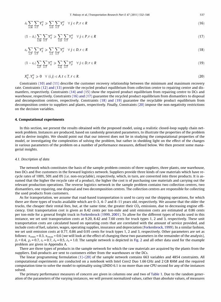
Constraints (10) and (11) describe the customer recovery relationship between the minimum and maximum recoveryrate. Constraints (12) and (13) provide the recycled product equilibrium from collection centre to repairing centre and dis-mantlers, respectively. Constraints (14) and (15) show the repaired product equilibrium from repairing centre to DCs andwarehouse, respectively. Constraints (16) and (17) guarantee the recycled product equilibrium from dismantlers to disposaland decomposition centres, respectively. Constraints (18) and (19) guarantee the recyclable product equilibrium fromdecomposition centre to suppliers and plants, respectively. Finally, Constraints (20) impose the non-negativity restrictionson the decision variables.

4. Computational experiments

In this section, we present the results obtained with the proposed model, using a realistic closed-loop supply chain net-work problem. Instances are produced, based on randomly generated parameters, to illustrate the properties of the problemand to derive insights. We should point out that our interest does not lie in studying the computational properties of themodel, or investigating the complexities of solving the problem, but rather in shedding light on the effect of the changesin various parameters of the problem on a number of performance measures, defined below. We then present some mana-gerial insights.

4.1. Description of data

The network which constitutes the basis of the sample problem consists of three suppliers, three plants, one warehouse,two DCs and five customers in the forward logistics network. Suppliers provide three kinds of raw materials which have re-cycle rates of 100%, 50% and 0% (i.e. non-recyclable), respectively, which, in turn, are converted into three products. It is as-sumed that the higher the recycle rate of a product, the higher the cost is of purchasing raw materials and carrying out therelevant production operations. The reverse logistics network in the sample problem contains two collection centres, twodismantlers, one repairing, one disposal and two decomposition centres. The collection centres are responsible for collectingthe used products from customers.

As for transportation, we assume that road-based transportation is used to carry out the shipping operations, for whichthere are three types of trucks available which are 0–3, 4–7 and 8–11 years old, respectively. We assume that the older thetrucks, the cheaper their rental fees, but, at the same time, the greater their CO2 emissions, due to decreasing engine effi-ciency. Unit transportation cost is given as 8.42 cents per ton-mile and unit emission costs are estimated at 0.86 centsper ton-mile for a general freight truck in Forkenbrock (1999, 2001). To allow for the different types of trucks used in thisinstance, we set unit transportation costs at 9.20, 8.42 and 7.60 cents for truck types 1, 2 and 3, respectively. These unittransportation costs are calculated based on operating costs that are correlated with the amount of service provided, andinclude costs of fuel, salaries, wages, operating supplies, insurance and depreciation (Forkenbrock, 1999). In a similar fashion,we set unit emission costs at 0.77, 0.86 and 0.95 cents for truck types 1, 2 and 3, respectively. Other parameters are set asfollows: armin = 0.3, armax = 0.6 (we will look at the effect of changing these two parameters in the remainder of the analysis),br = 0.4, vr = 0.7, er = 0.7, d2 = 0.5, d3 = 1.0. The sample network is depicted in Fig. 2 and all other data used for the exampleproblem are given in Appendix A.

There are three types of products in the sample network for which the raw materials are acquired by the plants from thesuppliers. End-products are sent to customers either from the warehouses or the DCs.

The linear programming formulation (1)–(20) of the sample network contains 663 variables and 4854 constraints. Allcomputational experiments are conducted on a notebook with Intel Core2 Duo 1.66 GHz and 2 GB RAM and the requiredcomputation time to solve the model to optimality using LINDO 6.1 is no more than one CPU second for any of the instancessolved.

The primary performance measures of concern are given in columns one and two of Table 1. Due to the random gener-ation of the parameters of the varying instances, we will present normalized values, rather than absolute values, of measures

Suppliers Zone Plants Zone

Warehouse

DCs Zone

Customers Zone

Collection Centers Zone

Dismantlers Zone

Disposal

Decomposition Centers Zone

Repairing Center

Forward Material FlowReverse Material Flow

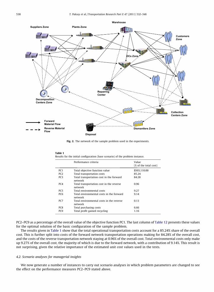
Fig. 2. The network of the sample problem used in the experiments.

Table 1Results for the initial configuration (base scenario) of the problem instance.

Performance criteria Value(% of the total cost)

PC1 Total objective function value $503,110.00PC2 Total transportation costs 85.24PC3 Total transportation cost in the forward

network84.28

PC4 Total transportation cost in the reversenetwork

0.96

PC5 Total environmental costs 9.27PC6 Total environmental costs in the forward

network9.14

PC7 Total environmental costs in the reversenetwork

0.13

PC8 Total purchasing costs 6.66PC9 Total profit gained recycling 1.16

538 T. Paksoy et al. / Transportation Research Part E 47 (2011) 532–546

PC2–PC9 as a percentage of the overall value of the objective function PC1. The last column of Table 12 presents these valuesfor the optimal solution of the basic configuration of the sample problem.

The results given in Table 1 show that the total operational transportation costs account for a 85.24% share of the overallcost. This is further split into costs of the forward network transportation operations making for 84.28% of the overall cost,and the costs of the reverse transportation network staying at 0.96% of the overall cost. Total environmental costs only makeup 9.27% of the overall cost, the majority of which is due to the forward network, with a contribution of 9.14%. This result isnot surprising, given the relative importance of the estimated unit cost values used in the tests.

4.2. Scenario analyses for managerial insights

We now generate a number of instances to carry out scenario analyses in which problem parameters are changed to seethe effect on the performance measures PC2–PC9 stated above.

T. Paksoy et al. / Transportation Research Part E 47 (2011) 532–546 539

4.2.1. Effect of changing demandsThe first scenario to consider is the effect of increasing demands of the products on the performance measures PC2–PC8.

We look at two of the products representing the two extremes in terms of recycling rates: the product with a 100% recyclerate and the product with a 0% recycle rate. Demands, as presented in Table A8 in the Appendix A, are increased by the per-centages shown in Table 2 for each scenario.

We present the results of Scenario 1 in Tables 3 and 4. The former presents normalized values for each performance mea-sure with respect to the base scenario of Table 1. In the latter, we present, for each scenario, the relative importance of eachperformance measure as a fraction of the total cost value.

The results presented in Tables 3 and 4 have the following implications: First, for the fully reusable product, the increasein demand results in an increase both in forward and reverse transportation costs. Similar changes are observed with theenvironmental costs. Although these results are rather intuitive and are as expected, this is not the case as far as the resultsgiven in Table 4 are concerned. Here, the relative importance of PC2 is seen to decrease with increasing values of demand,whereas the relative importance of PC5 is increasing under the same circumstances, with respect to the overall cost value.This suggests that, for reusable products, increasing demand through activities such as marketing will lessen the importanceof operational costs and place more emphasis on the environmental costs of the forward transportation activities. As for non-reusable products, similar results hold as far as Table 3 is concerned, but opposite results are obtained when one looks at therelative importance of the performance measures in Table 4. One possible reason for this is the fact that, due to the productbeing non-recyclable, no reverse operations are required, as demand is met only through the forward network.

Increasing demand seems to affect the purchasing cost of the recyclable product twice as much as that of the non-recy-clable product. However, with increased demand, the relative importance of the former increases, whereas that of the latterdecreases.

4.2.2. Effect of different product types and return ratesA closed-supply chain might be applicable for distribution and collection of a variety of products, ranging from books and

greeting cards to printers, automotive parts and computers. Differentiation between these products in the context of reverseflows can be made with regards to their return percentages. Rogers and Tibben-Lembke (1998) present sample statistics onthe return percentages of a number of different products, and indicate that return rates vary from as little as 4% to as high as

Table 2Scenarios for increasing demands.

Scenario Set 1 Customer demand Customer demand Customer demand100% Recyclable product 50% Recyclable product 0% Recyclable product

1 +2% +0% +0%2 +4% +0% +0%3 +6% +0% +0%4 +0% +0% +2%5 +0% +0% +4%6 +0% +0% +6%

Table 3Results for Scenario 1 normalized against the base scenario.

Scenario Set 1 PC2 PC3 PC4 PC5 PC6 PC7 PC8 PC9

1 0.9998 0.9999 0.9896 0.9968 0.9989 0.8462 1.0015 0.99142 1.0078 1.0079 0.9976 1.0049 1.0070 0.8530 1.0127 0.99083 1.0158 1.0161 0.9951 1.0305 1.0330 0.8599 1.0224 0.99004 1.0003 1.0003 1.0000 0.9978 1.0000 0.8461 0.9955 0.99135 1.0087 1.0088 0.9976 1.0048 1.0070 0.8530 0.9990 0.99946 1.0172 1.0173 1.0056 1.0129 1.0151 0.8599 1.0025 0.9987

Table 4Relative importance of performance measures as a fraction of total cost under Scenario 1.

Scenario Set 1 PC1 PC2 PC3 PC4 PC5 PC6 PC7 PC8 PC9

1 507243.20 85.22 84.27 0.95 9.24 9.13 0.11 6.67 1.152 511376.20 85.21 84.26 0.95 9.24 9.13 0.11 6.69 1.143 515509.40 85.20 84.26 0.94 9.40 9.29 0.11 6.70 1.134 507226.60 85.27 84.31 0.96 9.25 9.14 0.11 6.63 1.155 511343.00 85.29 84.34 0.95 9.24 9.13 0.11 6.60 1.156 515460.20 85.32 84.37 0.95 9.24 9.13 0.11 6.57 1.14

540 T. Paksoy et al. / Transportation Research Part E 47 (2011) 532–546

50%. Similar statistics are given by Srivastava (2008) for various product categories, including televisions, passenger cars, cel-lular handsets and computers, for which estimated return rates range between 20.6% and 30.7%. A particular case study pre-sented by Davey et al. (2005) quotes a return percentage of 5.7% of units shipped for inkjet printers, whereas another casestudy by de Koster et al. (2005), looking at large white goods, indicates this might be as high as 85%. To consider this productvariety in the return percentage in our analyses, we have performed additional tests with varying armin and armax values, cor-responding to minimum and maximum collection rates. Table 5 presents statistics where these values are set relatively high,as in the case of white goods. For this analysis, transportation capacities of the problem instance have been increased to re-flect the increments in the collection rates. Table 6 looks at the case where the collection rates are small, as in the case ofprinters, above, or the auto industry (Rogers and Tibben-Lembke, 1998).

Transportation costs of products with a small return percentage in the reverse network are small, as the results in Table 6show, constituting about 0.18% of the overall cost. On the other hand, the corresponding environmental cost is rather insig-nificant, with values around 0.02% of the overall cost. As for items with a higher return percentage, the reverse transportationcosts increase, as expected. They constitute around 1.54% of the overall costs, and this is a 62% increase as compared to thebase scenario. This table also shows a similar increase of 62% over the base scenario on the environmental cost of the reverselogistics network.

4.2.3. Effect of changing profitsThe third scenario to be investigated in this section pertains to the unit profits of the recyclable products. By problem

definition, it is assumed that product profits increase with the recyclability rate of the product, with the assumption thatthe reusable components will reduce the costs of raw material outsourcing. This is why the Scenario Set 2 given in Table7 does not include any analysis for the non-reusable product in the data set. As can be seen from this table, the goal of Sce-nario Set 2 is to study the effect of an increase in the unit profits, from 15% to 60%, in increments of 15%.

The results of this experiment are given in Tables 8 and 9 in a manner similar to Tables 3 and 4.Tables 8 and 9 imply that as the profits increase, there is not very much change in the operational and environmental

costs of transportation. The total profit PC9 shows an increase between 11% and 46% depending on the nature of the productconsidered, resulting in a decrease in the total cost value denoted by PC1. Of notable importance, both the values and the

Table 5Relative importance of performance measures as a fraction of total cost for armin = 0.8, armax = 0.9.

Scenario Set 1 PC1 PC2 PC3 PC4 PC5 PC6 PC7 PC8 PC9

1 510184.80 85.33 83.79 1.54 9.25 9.08 0.17 6.64 1.232 514350.00 85.32 83.78 1.54 9.24 9.07 0.17 6.65 1.223 518515.20 85.30 83.77 1.53 9.24 9.07 0.17 6.66 1.214 510161.20 85.37 83.83 1.54 9.26 9.08 0.18 6.59 1.235 514302.70 85.40 83.86 1.54 9.26 9.08 0.18 6.56 1.226 518444.20 85.42 83.89 1.53 9.25 9.08 0.17 6.53 1.21

Table 6Relative importance of performance measures as a fraction of total cost for armin = 0.04, armax = 0.08.

Scenario Set 1 PC1 PC2 PC3 PC4 PC5 PC6 PC7 PC8 PC9

1 507514.20 84.41 84.23 0.18 9.15 9.13 0.02 6.67 0.232 511641.30 84.39 84.22 0.17 9.14 9.12 0.02 6.69 0.233 515768.40 84.40 84.22 0.18 9.13 9.11 0.02 6.70 0.234 507494.20 84.44 84.27 0.17 9.15 9.13 0.02 6.63 0.235 511601.40 84.47 84.30 0.17 9.15 9.13 0.02 6.59 0.226 515708.50 84.50 84.33 0.17 9.14 9.12 0.02 6.57 0.22

Table 7Scenarios for increasing profits.

ScenarioSet 2

Unit profit of 100%recyclable product

Unit profit of 50%recyclable product

1 +15% +0%2 +30% +0%3 +45% +0%4 +60% +0%5 +0% +15%6 +0% +30%7 +0% +45%8 +0% +60%

Table 8Results for Scenario 2 normalized against the base scenario.

Scenario Set 2 PC2 PC3 PC4 PC5 PC6 PC7 PC8 PC9

1 1.0015 1.0012 1.0313 1.0000 1.0011 0.9231 1.0015 1.13792 1.0015 1.0012 1.0299 1.0009 1.0020 0.9219 1.0017 1.23983 1.0016 1.0013 1.0286 1.0007 1.0018 0.9207 1.0020 1.35004 1.0016 1.0013 1.0273 1.0005 1.0017 0.9196 1.0022 1.46005 1.0013 1.0013 1.0009 0.9998 1.0020 0.8469 1.0009 1.02686 1.0013 1.0013 1.0006 0.9995 1.0017 0.8466 1.0006 1.06107 1.0012 1.0012 1.0002 0.9992 1.0013 0.8463 1.0017 1.08658 1.0012 1.0012 0.9999 0.9999 1.0021 0.8461 1.0014 1.1119

Table 9Relative importance of performance measures as a fraction of total cost under Scenario 2.

Scenario Set 2 PC1 PC2 PC3 PC4 PC5 PC6 PC7 PC8 PC9

1 502480.80 85.37 84.38 0.99 9.27 9.15 0.12 6.67 1.322 501846.20 85.48 84.49 0.99 9.29 9.17 0.12 6.68 1.443 501211.60 85.59 84.60 0.99 9.30 9.18 0.12 6.69 1.574 500577.00 85.70 84.71 0.99 9.31 9.19 0.12 6.70 1.705 502939.10 85.27 84.31 0.96 9.26 9.15 0.11 6.66 1.196 502768.10 85.30 84.34 0.96 9.26 9.15 0.11 6.66 1.237 502597.20 85.32 84.36 0.96 9.26 9.15 0.11 6.67 1.268 502426.20 85.35 84.39 0.96 9.27 9.16 0.11 6.67 1.29

T. Paksoy et al. / Transportation Research Part E 47 (2011) 532–546 541

relative importance of the forward transportation activities increase with increasing profits. This is mainly due to the for-ward network being fed by the reverse network with recycled products.

4.2.4. Effect of changing transportation capacitiesThis section presents scenarios looking at changes in transportation capacities on links in the network and their effect on

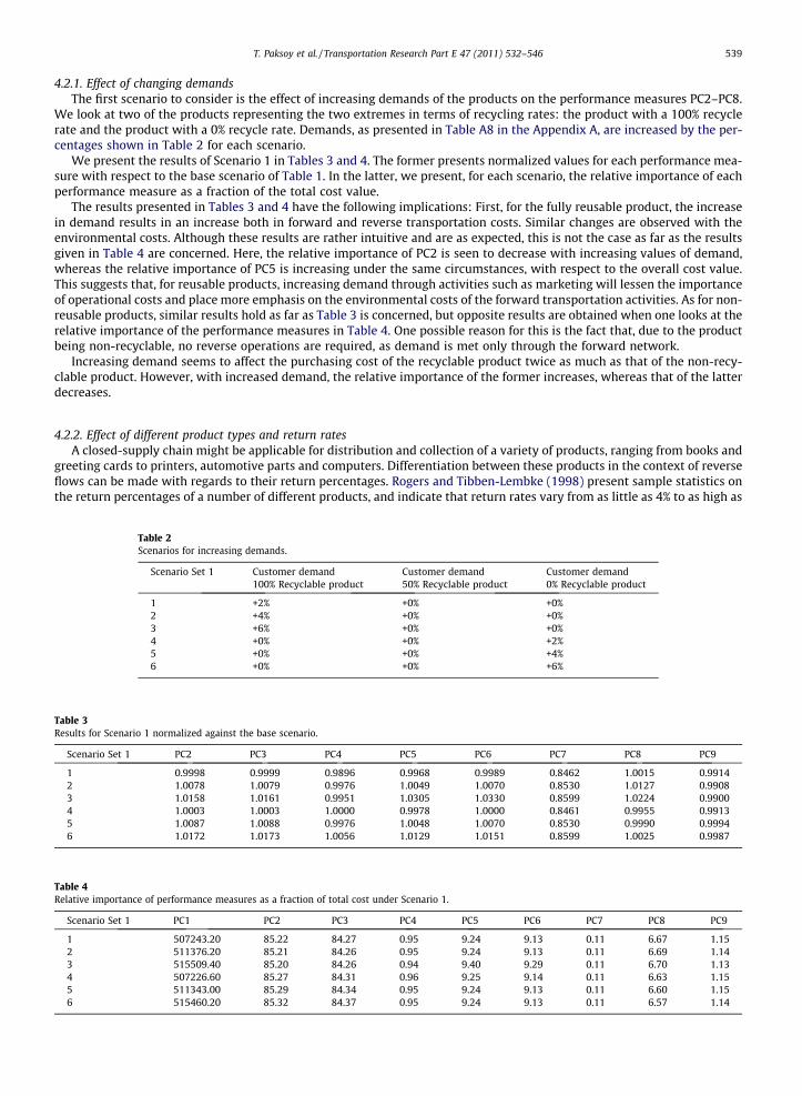
the performance measures. For this purpose, we gradually increase the capacity of a particular truck in increments of 15%and up to 60%, one truck at a time, while the capacities of the remaining trucks are kept constant. The relevant scenariosare presented in Table 10, while the associated results are given in Tables 11 and 12.

The results given in Table 11 have a number of implications. First, increasing the transportation capacity of Truck 1 doesnot seem to have a major impact on the performance measures, except for the slight decrease in PC5 of up to 1%. Similarmodifications in capacities of Trucks 2 and 3 yield more significant changes in PC1 and PC5. For the latter, a decrease ofup to 4% in operational costs (PC1) may be observed, but this comes at an increase of up to 2% in environmental costs(PC5) when capacities are gradually increased. These results suggest that shifting freight onto operationally less costly(but environmentally more hazardous) means of transportation have double the impact on operational costs as comparedto environmental costs. Measures PC8 and PC9 do not change much under the changes in transportation capacity.

As for Table 12, the results given therein are similar to those in Tables 3 and 9 in terms of the relative importance of thevarious performance measures with respect to total cost.

4.2.5. Effect of changing emission ratesThe last set of scenarios to be investigated is those relevant to changing emission rates of the three different truck types in

the sample network instance. To this end, emission rates are increased by units of 100%, up to 400%, for one truck at a time.The relevant scenarios are presented in Table 13 and the results given in Tables 14 and 15.

Table 10Scenarios for increasing transportation capacities.

Scenario Set 3 Truck 1 capacity (%) Truck 2 capacity (%) Truck 3 capacity (%)

1 +15 +0 +02 +30 +0 +03 +45 +0 +04 +60 +0 +05 +0 +15 +06 +0 +30 +07 +0 +45 +08 +0 +60 +09 +0 +0 +15

10 +0 +0 +3011 +0 +0 +4512 +0 +0 +60

Table 12Relative importance of performance measures as a fraction of total cost under Scenario 2.

Scenario Set 3 PC1 PC2 PC3 PC4 PC5 PC6 PC7 PC8 PC9

1 502325.60 85.24 84.28 0.96 9.24 9.13 0.11 6.67 1.162 501685.80 85.23 84.29 0.94 9.22 9.11 0.11 6.68 1.163 501045.80 85.26 84.30 0.96 9.20 9.09 0.11 6.69 1.164 500595.60 85.28 84.31 0.97 9.19 9.08 0.11 6.70 1.175 500990.40 85.17 84.21 0.96 9.30 9.19 0.11 6.69 1.166 498991.20 85.11 84.14 0.97 9.34 9.23 0.11 6.72 1.177 496993.00 85.03 84.06 0.97 9.40 9.28 0.12 6.74 1.188 495272.50 84.97 84.00 0.97 9.44 9.32 0.12 6.77 1.189 498724.00 85.04 84.08 0.96 9.39 9.28 0.11 6.72 1.17

10 494478.80 84.86 83.89 0.97 9.54 9.42 0.12 6.78 1.1811 491038.80 84.71 83.74 0.97 9.65 9.53 0.12 6.83 1.1912 488038.60 84.57 83.59 0.98 9.76 9.64 0.12 6.87 1.20

Table 13Scenarios for increasing transportation capacities.

Scenario Set 4 Truck 1 emission rate (%) Truck 2 emission rate (%) Truck 3 emission rate (%)

1 +100 +0 +02 +200 +0 +03 +300 +0 +04 +400 +0 +05 +0 +100 +06 +0 +200 +07 +0 +300 +08 +0 +400 +09 +0 +0 +100

10 +0 +0 +20011 +0 +0 +30012 +0 +0 +400

Table 11Results for Scenario 2 normalized against the base scenario.

Scenario Set 3 PC2 PC3 PC4 PC5 PC6 PC7 PC8 PC9

1 1.0000 1.0000 1.0000 0.9968 0.9989 0.8462 1.0015 1.00002 0.9986 0.9988 0.9779 0.9933 0.9954 0.8451 1.0017 0.99873 0.9977 0.9977 0.9975 0.9899 0.9920 0.8440 1.0019 0.99754 0.9970 0.9969 1.0069 0.9880 0.9900 0.8432 1.0025 1.00515 0.9965 0.9965 0.9973 1.0006 1.0028 0.8439 1.0018 0.99736 0.9918 0.9917 1.0037 1.0009 1.0031 0.8405 1.0023 1.00197 0.9869 0.9868 0.9997 1.0033 1.0045 0.9133 1.0013 1.00648 0.9828 0.9827 0.9962 1.0040 1.0054 0.9101 1.0022 1.00309 0.9905 0.9905 0.9928 1.0057 1.0080 0.8401 1.0018 1.0014

10 0.9800 0.9798 0.9946 1.0131 1.0145 0.9087 1.0021 1.001411 0.9715 0.9713 0.9877 1.0176 1.0192 0.9023 1.0025 1.002812 0.9639 0.9636 0.9918 1.0229 1.0247 0.8968 1.0022 1.0051

Table 14Results for Scenario 2 normalized against the base scenario.

Scenario Set 3 PC2 PC3 PC4 PC5 PC6 PC7 PC8 PC9

1 0.9858 0.9858 0.9896 1.1370 1.1400 0.9231 0.9865 0.98282 0.9857 0.9859 0.9719 1.2887 1.2938 0.9361 0.9867 0.97923 0.9865 0.9867 0.9747 1.4342 1.4400 1.0283 0.9866 0.97514 0.9888 0.9889 0.9763 1.5560 1.5633 1.0414 0.9851 0.97865 1.0009 1.0010 0.9927 1.1484 1.1514 0.9358 0.9864 0.98766 1.0008 1.0009 0.9875 1.3261 1.3314 0.9511 0.9855 0.97717 1.0008 1.0010 0.9815 1.5055 1.5121 1.0470 0.9857 0.97488 1.0008 1.0010 0.9860 1.6843 1.6931 1.0636 0.9853 0.97199 0.9997 0.9991 1.0505 1.2788 1.2835 0.9499 0.9858 0.9847

10 1.0179 1.0175 1.0540 1.3565 1.3620 0.9730 0.9860 0.972311 1.0303 1.0301 1.0490 1.4954 1.5026 0.9889 0.9860 0.978912 1.0303 1.0300 1.0545 1.6815 1.6899 1.0885 0.9855 0.9759

542 T. Paksoy et al. / Transportation Research Part E 47 (2011) 532–546

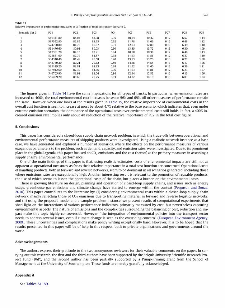
Table 15Relative importance of performance measures as a fraction of total cost under Scenario 2.

Scenario Set 3 PC1 PC2 PC3 PC4 PC5 PC6 PC7 PC8 PC9

1 510331.80 84.03 83.08 0.95 10.54 10.42 0.12 6.57 1.142 517552.90 82.85 81.93 0.92 11.78 11.66 0.12 6.48 1.123 524750.80 81.78 80.87 0.91 12.93 12.80 0.13 6.39 1.104 531476.60 80.93 80.03 0.90 13.85 13.72 0.13 6.30 1.095 517391.20 84.15 83.21 0.94 10.50 10.38 0.12 6.48 1.136 525851.60 82.79 81.87 0.92 11.93 11.81 0.12 6.37 1.107 534310.40 81.48 80.58 0.90 13.33 13.20 0.13 6.27 1.088 542769.20 80.21 79.32 0.89 14.68 14.55 0.13 6.17 1.069 525149.20 82.81 81.83 0.98 11.52 11.40 0.12 6.38 1.11

10 537912.60 82.32 81.36 0.96 11.93 11.81 0.12 6.23 1.0711 546705.90 81.98 81.04 0.94 12.94 12.82 0.12 6.13 1.0612 555499.20 80.68 79.75 0.93 14.32 14.19 0.13 6.03 1.04

T. Paksoy et al. / Transportation Research Part E 47 (2011) 532–546 543

The figures given in Table 14 have the same implications for all types of trucks. In particular, when emission rates areincreased to 400%, the total environmental cost increases between 56% and 69%. All other measures of performance remainthe same. However, when one looks at the results given in Table 15, the relative importance of environmental costs in theoverall cost function is seen to increase at most by about 4.7% relative to the base scenario, which indicates that, even underextreme emission scenarios, the dominance of the operational costs over environmental costs still holds. In fact, a 400% in-creased emission rate implies only about 4% reduction of the relative importance of PC2 in the total cost figure.

5. Conclusions

This paper has considered a closed-loop supply chain network problem, in which the trade-offs between operational andenvironmental performance measures of shipping products were investigated. Using a realistic network instance as a basecase, we have generated and explored a number of scenarios, where the effects on the performance measures of variousexogenous parameters to the problem, such as demand, capacity, and emission rates, were investigated. Due to its prominentplace in the global agenda, this paper focused on CO2 emissions, and the cost thereof, as the primary measures in assessing asupply chain’s environmental performance.

One of the main findings of this paper is that, using realistic estimates, costs of environmental impacts are still not asapparent as operational measures, as far as their relative importance in a total cost function are concerned. Operational costsof handling products, both in forward and reverse networks, seem to be dominant in all scenarios generated, including thosewhere emissions rates are exceptionally high. Another interesting result is relevant to the promotion of reusable products,the use of which seems to lessen the operational costs of the chain, but places a burden on the environmental costs.

There is growing literature on design, planning and operation of closed-loop supply chains, and issues such as energyusage, greenhouse gas emissions and climate change have started to emerge within the context (Ferguson and Souza,2010). This paper contributes to the literature by: (i) considering environmental costs within a closed-loop supply chainnetwork, mainly reflecting those of CO2 emissions due to transporting material in forward and reverse logistics networks,and (ii) using the proposed model and a sample problem instance, we present results of computational experiments thatshed light on the interactions of various performance indicators, primarily measured by cost, but nevertheless capturingenvironmental aspects. The nature of emissions and the complexities surrounding the balancing of cost, reduction and im-pact make this topic highly controversial. However, ‘‘the integration of environmental policies into the transport sectorneeds to address several issues, even if climate change is seen as the overriding concern’’ (European Environment Agency,2009). These uncertainties and complications make policy writing exceptionally hard. However, it is to be hoped that theresults presented in this paper will be of help in this respect, both to private organizations and governments around theworld.

Acknowledgements

The authors express their gratitude to the two anonymous reviewers for their valuable comments on the paper. In car-rying out this research, the first and the third authors have been supported by the Selçuk University Scientific Research Pro-ject Fund (BAP), and the second author has been partially supported by a Pump-Priming grant from the School ofManagement at the University of Southampton. These funds are hereby gratefully acknowledged.

Appendix A

See Tables A1–A9.

Table A1Distances (miles) in the forward network.

Plant 1 Plant 2 Plant 3

Supplier 1 250 190 380Supplier 2 220 410 250Supplier 3 190 290 310Warehouse 220 390 260Distribution Centre 1 120 100 135Distribution Centre 2 170 190 200

Table A2Distances (miles) in the forward network.

Warehouse Distribution Centre 1 Distribution Centre 2

Customer 1 240 170 220Customer 2 210 180 290Customer 3 190 210 200Customer 4 310 330 250Customer 5 280 150 280Warehouse – 140 110

Table A3Material handling capacities in the forward network (in tons).

Material type Suppliers Plants Warehouse DC

1 2 3 1 2 3 1 2

100% Recyclable 1000 900 1100 950 1150 1250 2200 1200 110050% Recyclable 1100 1000 1200 1050 1150 1150 1900 1000 900Non-recyclable 1200 1100 1300 1150 1050 1250 1800 1100 1100

Table A4Transportation capacities of each type of truck (in tons).

Truck types From suppliers From plants From warehouse From distribution centres

1 3200 3500 2200 18002 3400 3700 2100 17003 3100 3400 2300 1900

Table A5Distances (miles) in the reverse network.

Collection Centre 1 Collection Centre 2

Customer 1 6 8Customer 2 9 8.5Customer 3 7 10Customer 4 11 5Customer 5 12 13Repairing Centre 9 8Dismantler 1 9.5 12Dismantler 2 11 10

Table A6Distances (miles) in the reverse network.

Repairing Centre Dismantler 1 Dismantler 2

Warehouse 9DC 1 8DC 2 7Disposal 11 12Decomposition Centre 1 16 13Decomposition Centre2 15 19

544 T. Paksoy et al. / Transportation Research Part E 47 (2011) 532–546

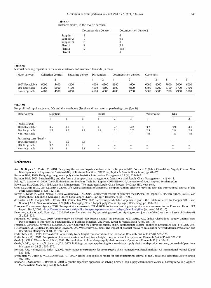
Table A7Distances (miles) in the reverse network.

Decomposition Centre 1 Decomposition Centre 2

Supplier 1 9 6Supplier 2 7 9.5Supplier 3 10 8Plant 1 11 7.5Plant 2 12 11.5Plant 3 9 8

Table A8Material handling capacities in the reverse network and customer demands (in tons).

Material type Collection Centres Repairing Centre Dismantlers Decomposition Centres Customers

1 2 1 2 1 2 1 2 3 4 5

100% Recyclable 6000 5400 4200 4000 4500 4600 4600 6000 4000 7000 5000 600050% Recyclable 5000 5500 4100 4500 4800 4800 4800 6700 5700 6700 5700 7700Non-recyclable 4500 4500 4050 4600 4000 4700 4700 5900 5900 6900 4900 5900

Table A9Net profits of suppliers, plants, DCs and the warehouse ($/unit) and raw material purchasing costs ($/unit).

Material type Suppliers Plants Warehouse DCs

1 2 3 1 2 3 1 1 2

Profits ($/unit)100% Recyclable 3.5 3.2 3.6 4 4.1 4.2 3.7 3.9 4.150% Recyclable 2.7 2.5 2.9 2.9 3.1 2.7 2.5 2.8 2.9Non-recyclable – – – – – – 1.9 1.8 1.9

Purchasing costs ($/unit)100% Recyclable 6 6.2 5.8 – – – – – –50% Recyclable 3.2 3.5 3 – – – – – –Non-recyclable 2.3 2 2.1 – – – – – –

T. Paksoy et al. / Transportation Research Part E 47 (2011) 532–546 545

References

Aras, N., Boyaci, T., Verter, V., 2010. Designing the reverse logistics network. In: in Ferguson, M.E., Souza, G.C. (Eds.), Closed-loop Supply Chains: NewDevelopments to Improve the Sustainability of Business Practices. CRC Press, Taylor & Francis, Boca Raton, pp. 67–97.

Beamon, B.M., 1999. Designing the green supply chain. Logistics Information Management 12 (4), 332–342.Beamon, B.M., 2008. Sustainability and the future of supply chain management. Operations and Supply Chain Management 1 (1), 4–18.Bektas�, T., Laporte, G., 2009. The Pollution-Routing Problem. Technical Report. CORMSIS-09-10, University of Southampton, Southampton.Bowersox, D.J., Closs, D.J., 1996. Logistical Management: The Integrated Supply Chain Process. McGraw-Hill, New York.Choi, B.C., Shin, H.S.S., Lee, S.Y., Hur, T., 2006. Life cycle assessment of a personal computer and its effective recycling rate. The International Journal of Life

Cycle Assessment 11 (2), 122–128.Davey, S., Guide Jr., V.D.R., Neeraj, K., Van Wassenhove, L.N., 2005. Commercial returns of printers: the HP case. In: Flapper, S.D.P., van Nunen, J.A.E.E., Van

Wassenhove, L.N. (Eds.), Managing Closed Loop Supply Chains. Springer, Heidelberg, pp. 87–96.de Koster, R.B.M., Flapper, S.D.P., Krikke, H.R., Vermeulen, W.S., 2005. Recovering end-of-life large white goods: the Dutch initiative. In: Flapper, S.D.P., van

Nunen, J.A.E.E., Van Wassenhove, L.N. (Eds.), Managing Closed Loop Supply Chains. Springer, Heidelberg, pp. 169–181.European Environment Agency, 2009. Transport at a crossroads, TERM 2008: indicators tracking transport and environment in the European Union. EEA

Report, No. 3/2009. <http://www.eea.europa.eu/publications/transport-at-a-crossroads/at_download/file> (accessed 06.12.10).Fagerholt, K., Laporte, G., Norstad, I., 2010. Reducing fuel emissions by optimizing speed on shipping routes. Journal of the Operational Research Society 61

(3), 523–529.Ferguson, M., Souza, G.C., 2010. Commentary on closed-loop supply chains. In: Ferguson, M.E., Souza, G.C. (Eds.), Closed-loop Supply Chains: New

Developments to Improve the Sustainability of Business Practices. CRC Press, Taylor & Francis, Boca Raton, pp. 1–6.Ferretti, I., Zanoni, S., Zavanella, L., Diana, A., 2007. Greening the aluminum supply chain. International Journal Production Economics 108 (1–2), 236–245.Fleischmann, M., Beullens, P., Bloemhof-Ruwaard, J.M., Wassenhove, L., 2001. The impact of product recovery on logistics network design. Production and

Operations Management 10 (3), 156–173.Forkenbrock, D.J., 1999. External costs of intercity truck freight transportation. Transportation Research Part A 33 (7–8), 505–526.Forkenbrock, D.J., 2001. Comparison of external costs of rail and truck freight transportation. Transportation Research Part A 35 (4), 321–337.Guide Jr., V.D.R., Wassenhove, L.N.V., 2009. The evolution of closed-loop supply chain research. Operations Research 57 (1), 10–18.Guide, V.D.R., Jayaraman, V., Jonathan, D.L., 2003. Building contingency planning for closed-loop supply chains with product recovery. Journal of Operations

Management 21 (3), 259–279.Hervani, A.A., Helms, M.M., Sarkis, J., 2005. Performance measurement for green supply chain management. Benchmarking: An International Journal 12 (4),

330–353.Jayaraman, V., Guide Jr., V.D.R., Srivastava, R., 1999. A closed-loop logistics model for remanufacturing. Journal of the Operational Research Society 50 (5),

497–508.Kannan, G., Sasikumar, P., Devika, K., 2010. A genetic algorithm approach for solving a closed loop supply chain model: a case of battery recycling. Applied

Mathematical Modelling 34 (3), 655–670.

546 T. Paksoy et al. / Transportation Research Part E 47 (2011) 532–546

Krikke, H., Bloemhof-Ruwaard, J., Van Wassenhove, L., 2001. Design of closed-loop supply chains: a production and return network for refrigerators. ERIMReport Series Research in Management, ERS-2001-45-LIS, Erasmus Research Institute of Management, Rotterdam, The Netherlands.

Krikke, H., Bloemhof-Ruwaard, J., Van Wassenhove, L., 2003. Concurrent product and closed-loop supply chain design with an application to refrigerators.International Journal of Production Research 41 (16), 3689–3719.

Meixell, M.J., Gargeya, V.B., 2005. Global supply chain design: a literature review and critique. Transportation Research Part E 41 (6), 531–550.Min, H., Ko, C.S., Ko, H.J., 2006. The spatial and temporal consolidation of returned products in a closed-loop supply chain network. Computers and Industrial

Engineering 51 (2), 309–320.Neto, J.Q.F., Bloemhof-Ruwaard, J.M., Van Nunen, J.A.E.E., Van Heck, E., 2008. Designing and evaluating sustainable logistics networks. International Journal

Production Economics 111 (2), 195–208.Rogers, D.S., Tibben-Lembke, R.S., 1998. Going backwards: reverse logistics trends and practices. Reverse Logistics Executive Council. <http://www.rlec.org/

reverse.pdf> (accessed 06.12.10).Sarkis, J., 2003. A strategic decision framework for green supply chain management. Journal of Cleaner Production 11 (4), 397–409.Sheu, J.B., Chou, Y.H., Hu, C., 2005. An integrated logistic operational model for green supply chain management. Transportation Research Part E 41 (4), 287–

313.Srivastava, S.K., 2007. Green supply-chain management: a state-of-the-art literature review. International Journal of Management Reviews 9 (1), 53–80.Srivastava, S.K., 2008. Network design for reverse logistics. Omega 36 (4), 535–548.Wang, H.-S., Hsu, H.-W., 2010. A closed-loop logistic model with a spanning tree based genetic algorithm. Computers & Operations Research 37 (2), 376–

389.Yang, G., Wang, Z., Li, X., 2009. The optimization of the closed-loop supply chain network. Transportation Research Part E 45 (1), 16–28.Zhu, Q.H., Sarkis, J., Lai, K.H., 2008. Green supply chain management implications for ‘‘closing the loop’’. Transportation Research Part E 44 (1), 1–18.