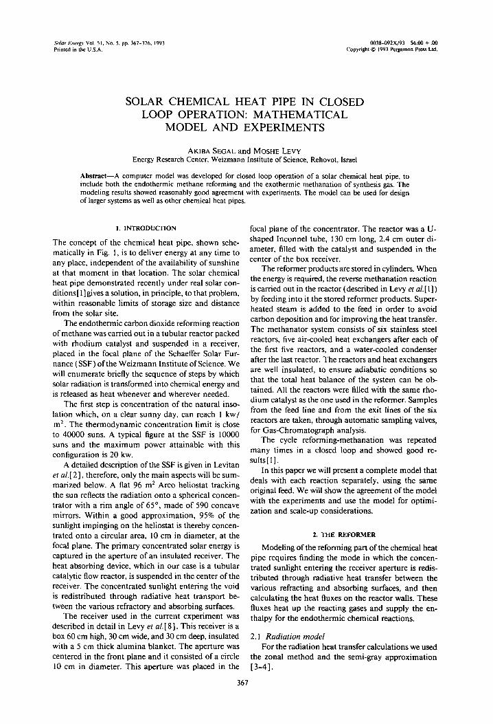
Solar Energy Vol. 5 I, No. 5, pp. 367-376, 1993 0038-092X/93 $6.00 + .00 Printed in the U.S.A. Copyright © 1993 Pergamon Press Ltd.

SOLAR CHEMICAL HEAT PIPE IN CLOSED LOOP OPERATION: MATHEMATICAL

MODEL AND EXPERIMENTS

AKIBA SEGAL and MOSHE LEVY Energy Research Center, Weizmann Institute of Science, Rehovot, Israel

Abstract--A computer model was developed for closed loop operation of a solar chemical heat pipe, to include both the endothermic methane reforming and the exothermic methanation of synthesis gas. The modeling results showed reasonably good agreement with experiments. The model can be used for design of larger systems as well as other chemical heat pipes.

1. I N T R O D U C T I O N

The concept of the chemical heat pipe, shown sche- matically in Fig. 1, is to deliver energy at any time to any place, independent of the availability of sunshine at that moment in that location. The solar chemical heat pipe demonstrated recently under real solar con- ditions [ 1 ] gives a solution, in principle, to that problem, within reasonable limits of storage size and distance from the solar site.

The endothermic carbon dioxide reforming reaction of methane was carded out in a tubular reactor packed with rhodium catalyst and suspended in a receiver, placed in the focal plane of the Schaeffer Solar Fur- nance (SSF) of the Weizmann Institute of Science. We will enumerate briefly the sequence of steps by which solar radiation is transformed into chemical energy and is released as heat whenever and wherever needed.

The first step is concentration of the natural inso- lation which, on a clear sunny day, can reach 1 kw/ m 2. The thermodynamic concentration limit is close to 40000 suns. A typical figure at the SSF is 10000 suns and the maximum power attainable with this configuration is 20 kw.

A detailed description of the SSF is given in Levitan et a/.[2], therefore, only the main aspects will be sum- marized below. A fiat 96 m 2 Arco heliostat tracking the sun reflects the radiation onto a spherical concen- trator with a rim angle of 65 °, made of 590 concave mirrors. Within a good approximation, 95% of the sunlight impinging on the heliostat is thereby concen- trated onto a circular area, 10 cm in diameter, at the focal plane. The primary concentrated solar energy is captured in the aperture of an insulated receiver. The heat absorbing device, which in our case is a tubular catalytic flow reactor, is suspended in the center of the receiver. The concentrated sunlight entering the void is redistributed through radiative heat transport be- tween the various refractory and absorbing surfaces.

The receiver used in the current experiment was described in detail in Levy el a/.[8]. This receiver is a box 60 cm high, 30 cm wide, and 30 cm deep, insulated with a 5 cm thick alumina blanket. The aperture was centered in the front plane and it consisted of a circle l0 cm in diameter. This aperture was placed in the

focal plane of the concentrator. The reactor was a U- shaped Inconnel tube, 130 cm long, 2.4 cm outer di- ameter, filled with the catalyst and suspended in the center of the box receiver.

The reformer products are stored in cylinders. When the energy is required, the reverse methanation reaction is carried out in the reactor (described in Levy et al. [ l ] ) by feeding into it the stored reformer products. Super- heated steam is added to the feed in order to avoid carbon deposition and for improving the heat transfer. The methanator system consists of six stainless steel reactors, five air-cooled heat exchangers after each of the first five reactors, and a water-cooled condenser after the last reactor. The reactors and heat exchangers are well insulated, to ensure adiabatic conditions so that the total heat balance of the system can be ob- tained. All the reactors were filled with the same rho- dium catalyst as the one used in the reformer. Samples from the feed line and from the exit lines of the six reactors are taken, through automatic sampling valves, for Gas-Chromatograph analysis.

The cycle reforming-methanation was repeated many times in a closed loop and showed good re- suits [1 ].

In this paper we will present a complete model that deals with each reaction separately, using the same original feed. We will show the agreement of the model with the experiments and use the model for optimi- zation and scale-up considerations.

2. THE R E F O R M E R

Modeling of the reforming part of the chemical heat pipe requires finding the mode in which the concen- trated sunlight entering the receiver aperture is redis- tributed through radiative heat transfer between the various refracting and absorbing surfaces, and then calculating the heat fluxes on the reactor walls. These fluxes heat up the reacting gases and supply the en- thalpy for the endothermic chemical reactions.

2. l R a d i a t i o n m o d e l For the radiation heat transfer calculations we used

the zonal method and the semi-gray approximation [3-4].

367

368 A. SEGAL a n d M . LEVY

STORAGE

STORAGE

Fig. 1. A schematic presentation of the solar chemical heat pipe concept.

In the zonal method the internal surface of the re- ceiver and the external surface of the reactor are divided into surface elements sufficiently small to be considered isothermal and equi-energetic. The view factors be- tween each pair of surface elements were calculated using the computer package VIEW [ 5 ]. For these cal- culations all surfaces must be planar, therefore the re- actor tube circumference was approximated by a hex- agonal polygon. The computer time required for these calculations depends on the number of zones, and may be rather long. However, the view factors have to be calculated only once for a given receiver geometry.

In the semi-gray approximation one absorptivity is used for incident solar radiation and another one for radiation originating by emission, within the enclosure. Thus, two independent energy balances are obtained.

The first energy balance is for the visible spectrum coming from the sun (superscript VI):

- .i v l q ~ J J=' [a). t - Fk-j ~'-7 ]qJ =

( k = 1 , 2 . . . . . N ) . (1)

In order to solve this system we must know the s lar flux ~o~ direct o es qk , on each k-surface of the receiver

and the reactor. These fluxes are calculated beginning with calculation of sun images generated in the focal plane by individual mirror facets of the concentrator. The convoluted image is then projected onto all the zones of the receiver and the reactor exposed to direct radiation. The total energy entering the receiver is cal- culated using a scaling procedure based on the exper- imentally determined energy absorbed by the reacting gases and the calculated receiver efficiency [ 6 ].

The second energy balance refers to the energy emitted in the infrared spectrum (superscript IR) . This energy includes the infrared radiation and the emitted thermal radiation. In terms of the radiosities in the infrared spectrum qO.tR, this energy balance is expressed by the following system of equations:

N

[~kj - - F k - j ( 1 -- a~R)]q) ''R = al,tR aTk4 j=l

( k = 1,2 . . . . . M) (2a)

N

[Fk- j - 5 j q y R = qk - q~k q j=l

( k = M + 1 . . . . . N). ( 2 6 )

Equation (2a) was assigned to surfaces where the temperatures were known and eqn (2b) was assigned to surfaces where the net radiation fluxes could be evaluated.

• The unknown total fluxes could then be calculated from:

IR

q, = q~', + ~ (q~,ln _ a T e ) 1 - - o l k

( k = 1,2 . . . . . M) (3)

and the unknown temperatures were calculated from:

Tk = [6kj -- (1 -- a~R)Fk_j] O.---"~kR]

( k = M + 1 . . . . . N). (4)

The heat losses considered in the heat transfer cal- culations were by radiation, conduction through the receiver walls, and natural convection. 1. Radiation losses through the receiver aperture were

calculated by summation of the product qkAk, where qs are the total fluxes on the aperture and As are their corresponding areas. The ks in this case, refer to all surface elements of the aperture. Preliminary calculations showed that radiation losses, in the temperature range under study, amount to about 19% of the total solar energy entering the receiver aperture.

2. Conduction losses through receiver walls were cal- culated by considering that the net flux on a surface element of the wall is given by:

ke (T~ ,au , i _ T~'".o) qk = " f f (5)

where superscript (wall,i) refers to the interior side and (wall,o) to the exterior side of the receiver wall. This flux, lost to the environment by radiation and convection, is calculated by:

qk = (hr + he)( T g ~"'° - T~mb) (6a)

where hr, the radiation heat transfer coefficient is:

ecr( ( Tga"'°) 4 - (Tamb) 4) hr = T g ~" ' ° - Tar,,b (6b)

From eqns (5) and (6a), T g a"'° and the flux loss by conduction on surface k can be determined. This will be the net flux for this surface. The total loss by conduction through the receiver walls was esti- mated to about 21% of the solar energy entering the receiver aperture.

Solar chemical heat pipe 369

3. Natural convection losses through the aperture were calculated using the empirical correlation given by Boehm[ 7 ]:

q = 0.81(Trec - Tamb) 1'4 (7)

where T,~ is the average temperature of the receiver. Preliminary calculations showed that the heat loss by natural convection is in order of only 1% of the input energy in the receiver, and therefore it can be neglected for the present geometry.

As the sum of the losses amount to 41%, the net heat absorbed in the reactor is 59% of total energy input. This is the energy that is stored in the chem- ical reaction and in the sensible heat of the product gas mixture.

cation was imposed due to the complexity of the heat transfer calculations (by radiation inside the receiver combined with convection inside the reactor).

Nevertheless, the agreement between the model calculations and the experiments was satisfactory [ 8 ]. In subsection 2.5 an example as a validation of the model for such a calculation is presented.

2.3 Kinetics o f the reforming reactions The kinetics of the reaction are based on experi-

ments performed recently [ 8 ]. The rate equation for CO2 reforming of methane

is:

(x) (x) rtX) = k(X) Kco2KcH,Pco2Pc~,

(1 + vtx) D + t.-(x) o ~2 I~'CO2 j CO 2 g~'CH4 "l CH 4 ]

2.2 Heat transfer calculations inside the reactor From radiation calculations, performed for the re-

ceiver enclosure, the net heat fluxes on each reactor segment is obtained. These heat fluxes are used for the endothermic reforming reaction under study:

(P"2Pc°) 2 ] X I ~ ~-(~)I (9)

PCO21"CH, IX eu .I

and for the reverse water gas shift reaction the following rate equation was used:

CO2 + CH4 = 2CO + 2H2

which is always accompanied by the reverse water gas shift reaction:

CO2 + H2 = CO + H20

r ( y ) = k ( y ) .~(y) t... D o

/~ C O 2 / k i l l I CO2't H2 (I + (Y) t : (y)o ~2 Kco2Pco2 + ,. H2 "H21

Pco P.2o ] × 1 Pco, P . ~ K ~ ) j . (10)

The model used for this reactor is pseudohomo- geneous and unidimensional. The energy and mass balances at position z along the reactor tube are given by the following equations:

dx -_ onS r(X) (8a) dz Mi

dy = pBS r(y ) (8b) dz M~

The equilibrium constants were calculated from enthalpy data:

K ( X ) = e(34.15-31272/T) I((r) e(3.70-4088.2/T). eu --eq = (11)

The rate constants k m and the adsorbtion constants KI s) for absorption of component i in reaction s are of the form:

k ts) = A(S)e -E' ' /RT ..ir:(s) = AlS)e et' '/Rr. (12)

,i4;o ] dz = G-~p - on(r(X)H~X) + r(Y)H(Y)) " (8c)

For solving this ordinary differential equations system we used the finite difference method (see next section) and compared the results with calculations using the IMSL routines. The results were very close, however, the computation time was shorter for the former method. The output of the calculation included the wall and gas temperature profiles, gas composition, and various other parameters. The model for the reforming reaction takes into consideration the kinetic equations derived from the experimental work and new corre- lations for the convective heat transfer coefficient [ 8 ].

This one-dimensional model used for the reforming reaction neglects the resistance to heat and mass trans- fer in the radial direction and therefore predicts a uni- form temperature and conversion along the cross sec- tion of the reactor. This is obviously a simplification for reactions with large enthalpies, but this simplifi-

The values of constants A and E used were:

A (x) = 100 E (x) = 80000

A (X) ~ ( x ) co2 = 0.026 ~co2 = 37600

A ( y ) ~ ( y ) co2 = 0.58 "~co2 = 9300

A (y) = 350 E (~) = 81000

17 ' (x ) = A (c~, = 0.026 ,~c~ 40700

A~] = 1.5 E~r~ = 6000.

(For units see the Nomenclature section.) The effect of the nonuniformity in deposition of

catalyst on the alumina pellets (by a factor of effec- tiveness) and the mass transport effect (by a term for external diffusion ra) were taken into consideration. The final reaction rate is given by:

1 Tm 1 _is) rmtanh(Tm) + (13) [ f ina l re

370 A. SEGAL and M. LEVV

where s refers t o one of the four reactions considered (both in the reforming and methanation).

2.4 Computing method for convergence calculation To implement the general theory presented in this

study a computer package was constructed. This pack- age comprises of two program preprocessors (VIEW and MIRROR) and two programs, in mutual inter- action, treating, respectively, the radiative heat transfer within the receiver (SOLRAD) and the heat transfer, heating and chemistry of the reformer (REFMETH).

The preset data for SOLRAD are the view factors calculated by the preprocessor program VIEW and the direct solar fluxes on receiver walls, calculated by MIRROR. The calculations from SOLRAD provide the respective temperatures of these walls. For the re- actor surfaces, the temperatures are initially guessed at, and the calculations generate the net fluxes on each surface segment of reactor. These fluxes are the input for the chemistry program REFMETH.

The interface between the radiative program and the chemical program is through the wall temperature on each reactor segment, calculated by REFMETH. This program generates a temperature array on the reactor walls which is used as an improved boundary condition for SOLRAD for generating a new net heat flux vector. The latter constitutes an improved bound- ary condition for REFMETH and so on.

The criterion for convergence is set by defining a parameter S as:

S = ; ~ = t ( T ~ ( i + 1 ) - T ~ ' ( i ) ) 2

= A T " f M < T O L

where the index k counts the M surface elements along the reactor, i counts the iterations, and AT" is the average deviation of the wall temperature between two consecutive iterations. The value for the tolerance TOL is defined by the above inequality. For example, for 2°C, average permitted difference between reactor wall temperatures in two consecutive iterations TOL must be TOL ~ 2V-M.

We found that convergence efficiency is achieved faster by selectively adjusting the components of tem- perature array, which differ most from their respective values in the previous iteration. For example, if we decrease only one component of the guessed temper- ature vector on the reactor, this means that the emissive power will decrease on this segment. Consequently, the net heat flux will increase and, as a result, the ex- terior wall temperatures, calculated from REFMETH will increase. An adequate manipulation of this inter- action will lead to convergence. This is performed by determining the maximum I ATm~ ] deviation between wall reactor temperatures for each segment before and after iteration and adjusting those vector com- ponents with a deviation within the range of (0.7. • • 0.9)l A T ~ I. The correction is made with the

same value on all these segments but in a direction that the differences of temperatures between iterations decrease (i.e., if the temperature of the segment after iteration is higher than the previous temperature, the temperature of this reactor segment will be increased). The magnitude of the correction depends on the value of ]ATmax[. When IATma, I decreases under a fixed value, which depends on the problem's dimensionality, the magnitude of correction is decreased in order to prevent divergence. Toward the end of the convergence search, for example, when I AT,,~x] becomes of the order of 30-40°C, the corrective procedure is altered and all the components of vector temperature are cor- rected at once. The new deviant vector components are taken to be weighted averages between penultimate and ultimate values. By using this method, it is possible to obtain convergence either in case of a big number of segments in the reactor or when we do not have a good guess of the initial temperature vector.

In this mode, the calculation converges to a unique steady state solution and generates receiver wall tem- peratures, net heat flux profile, reactor wall temperature profile, catalytic bed temperatures, methane conver- sion, gas composition, and various other parameters.

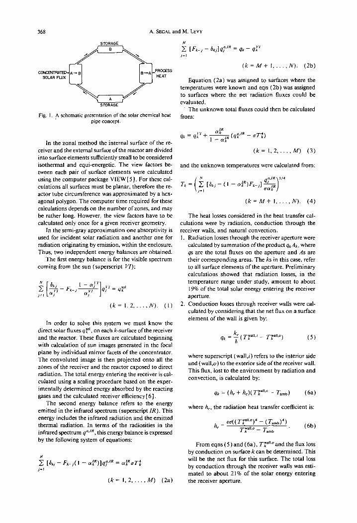
2.5 Comparison with experiment A representative example of the calculated tem-

perature profile is shown in Fig. 2. It can be seen that the agreement with the experimental points is quite good. The evolution of conversion along the reactor was only calculated, as gas samples along the reactor tube were not taken, and only the composition of the final product is an experimental point. This experi- mental % methane conversion of the product gas was used in order to calculate the power entering the re- ceiver. This power input was used in computations until superposition of experimental conversion on the calculated conversion was obtained. Estimated calcu- lations beginning with solar radiosity, measured in some experiments gave values which were very closed to the input power considered in each experiment. The

9 0 0 - ' ' ' ' I ' ' ' ' I ' ' ' ' I ' ' ' ' I ' ' ' "

8 O O p ,

7 0 0 / - . ~ 13 ~., ~ ~ X

~, 6 0 0 x.... , ~ "

5 0 0 ....- ~

400~-, , , , I , I ,,,I .... It ]I I

0 0 . 2 0 4 0 . 6 0 . 8

F r o c t i o n o l l eng th

Fig. 2. Compar ison o f exper imental and calculated wall and gas temperatures. The final calculated (exper imenta l ) gas composi t ion (%) was: C H 4 : 4 . 6 2 (4 .30) , H 2 0 : 4 . 4 8 (5 .00) , CO: 47.25 (44.50), H2:38.30 (34.30), and CO2:5.35 ( l 1.90).

Solar chemical heat pipe 371

54

"~ 36 o>

%

g 0

~ power

l i i l i , , i l , , , , l , , , , I ,

flow

I I I

0 0.5 1.0 1.5 2£) 25 Froction relolive to reference

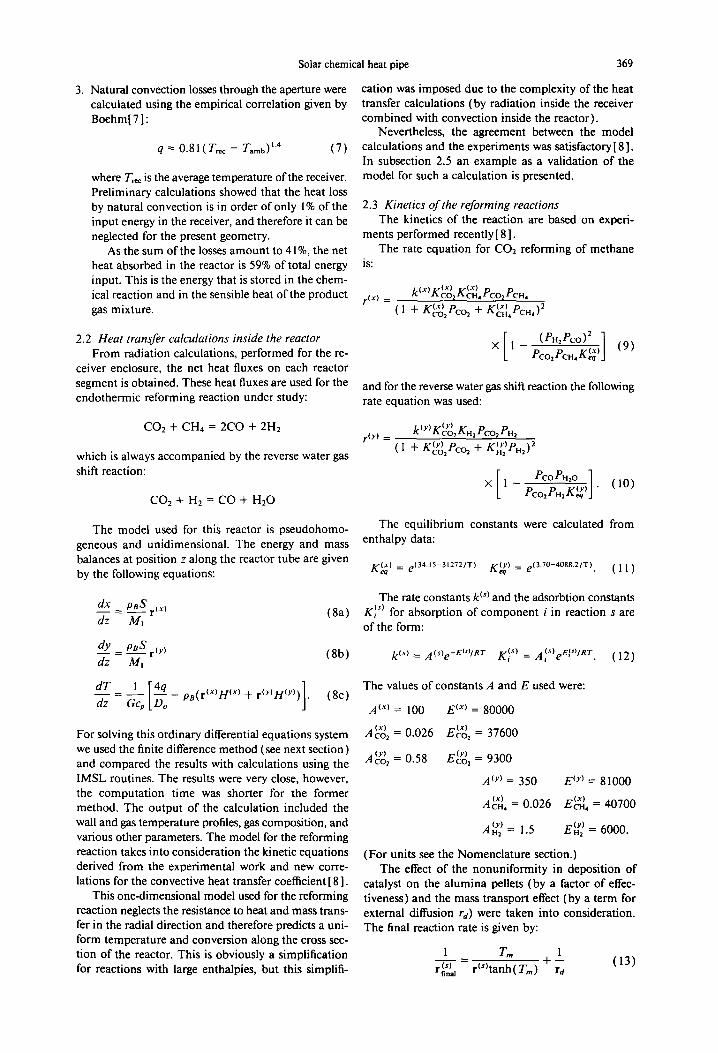
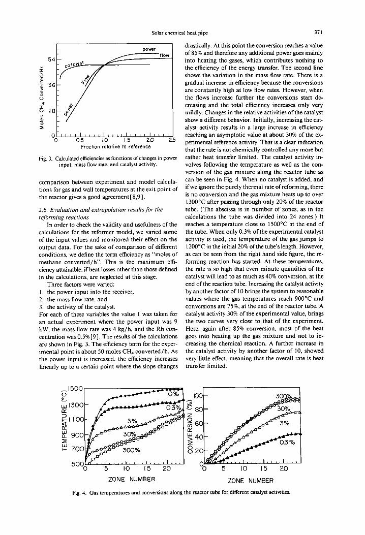
Fig. 3. Calculated ef~ciencies as functions ofchanges in power input, mass flow rate, and catalyst activity.

comparison between experiment and model calcula- tions for gas and wall temperatures at the exit point of the reactor gives a good agreement [ 8,9 ].

2.6 Evaluation and extrapolation results for the reforming reactions

In order to check the validity and usefulness of the calculations for the reformer model, we varied some of the input values and monitored their effect on the output data. For the sake of comparison of different conditions, we define the term efficiency as "moles of methane converted/h ' . This is the maximum effi- ciency attainable, if heat losses other than those defined in the calculations, are neglected at this stage.

Three factors were varied: I. the power input into the receiver, 2. the mass flow rate, and 3. the activity of the catalyst. For each of these variables the value 1 was taken for an actual experiment where the power input was 9 kW, the mass flow rate was 4 kg/h, and the Rh con- centration was 0.5% [ 9 ]. The results of the calculations are shown in Fig. 3. The efficiency term for the exper- imental point is about 50 moles CH4 converted/h. As the power input is increased, the efficiency increases linearly up to a certain point where the slope changes

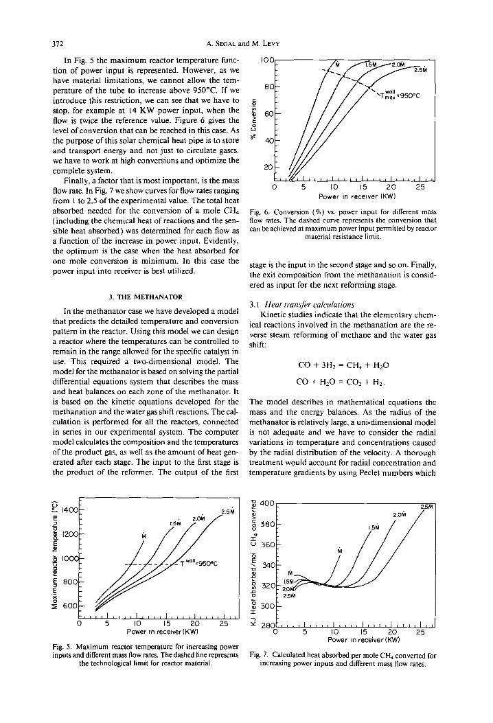
drastically. At this point the conversion reaches a value of 85% and therefore any additional power goes mainly into heating the gases, which contributes nothing to the efficiency of the energy transfer. The second line shows the variation in the mass flow rate. There is a gradual increase in efficiency because the conversions are constantly high at low flow rates. However, when the flows increase further the conversions start de- creasing and the total efficiency increases only very mildly. Changes in the relative activities of the catalyst show a different behavior. Initially, increasing the cat- alyst activity results in a large increase in efficiency reaching an asymptotic value at about 30% of the ex- perimental reference activity. That is a clear indication that the rate is not chemically controlled any more but rather heat transfer limited. The catalyst activity in- volves following the temperature as well as the con- version of the gas mixture along the reactor tube as can be seen in Fig. 4. When no catalyst is added, and if we ignore the purely thermal rate of reforming, there is no conversion and the gas mixture heats up to over 1300°C after passing through only 20% of the reactor tube. (The abscissa is in number of zones, as in the calculations the tube was divided into 24 zones.) It reaches a temperature close to 1500°C at the end of the tube. When only 0.3% of the experimental catalyst activity is used, the temperature of the gas jumps to 1200°C in the initial 20% of the tube's length. However, as can be seen from the right hand side figure, the re- forming reaction has started. At these temperatures, the rate is so high that even minute quantities of the catalyst will lead to as much as 40% conversion, at the end of the reaction tube. Increasing the catalyst activity by another factor of 10 brings the system to reasonable values where the gas temperatures reach 900°C and conversions are 75%, at the end of the reactor tube. A catalyst activity 30% of the experimental value, brings the two curves very close to that of the experiment. Here, again after 85% conversion, most of the heat goes into heating up the gas mixture and not to in- creasing the chemical reaction. A further increase in the catalyst activity by another factor of 10, showed very little effect, meaning that the overall rate is heat transfer limited.

~1500~

-, oo

~ 110C

~_ 900

UA

0,~6"..i, , , , I . , . . i . . . . I , . . 50 0 5 I 0 1.5 20

.~ 1(30-

80-

0 60 - 3°/o

nr" 401

z o 2o

c~ ;a~---~ . . . . t . . . . I , , , . I . , , 5 I0 15 20

ZONE NUMBER ZONE NUMBER

Fig. 4. Gas temperatures and conversions along the reactor tube for different catalyst activities.

372 A. SEGAL and M. LEVY

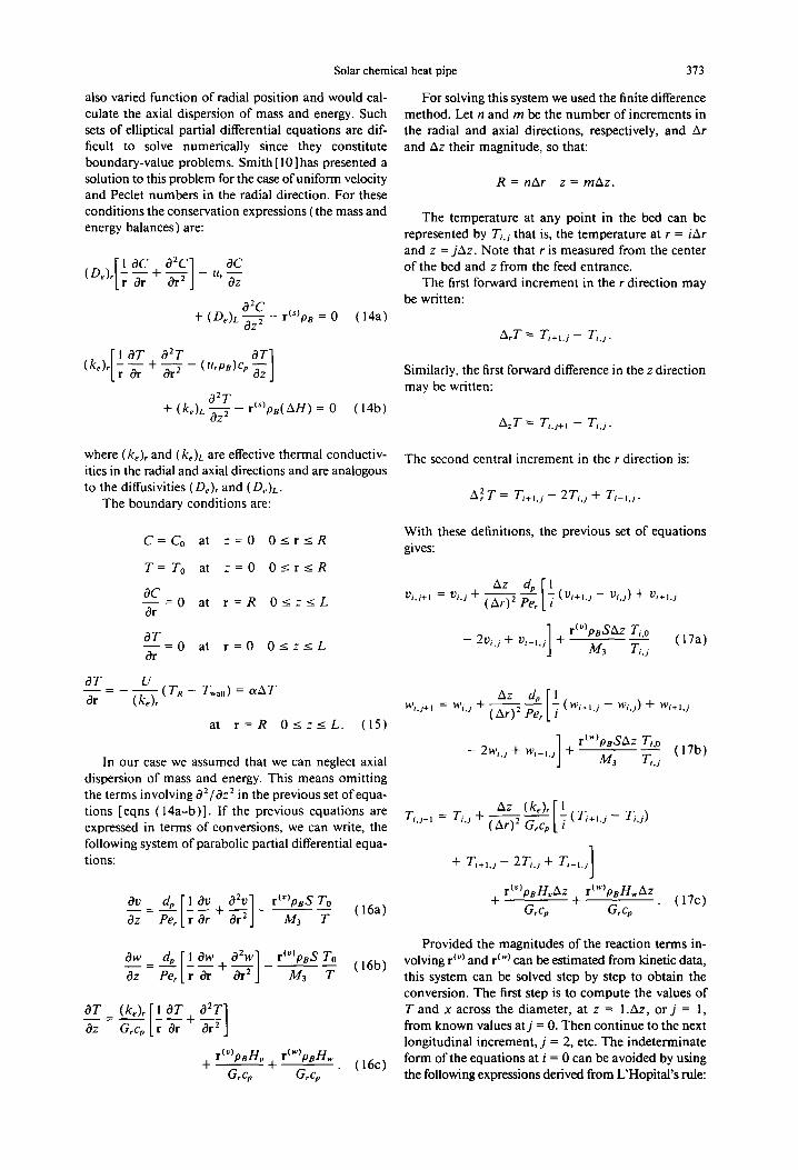
In Fig. 5 the m a x i m u m reactor t empera ture func- t ion of power input is represented. However, as we have material l imitat ions, we canno t allow the tem- perature of the tube to increase above 950°C. If we in t roduce this restriction, we can see tha t we have to stop, for example at 14 K W power input, when the flow is twice the reference value. Figure 6 gives the level of convers ion that can be reached in this case. As the purpose of this solar chemical heat pipe is to store and t ranspor t energy and not just to circulate gases, we have to work at high conversions and opt imize the complete system.

Finally, a factor tha t is most impor tan t , is the mass flow rate. In Fig. 7 we show curves for flow rates ranging from 1 to 2.5 of the exper imental value. The total heat absorbed needed for the convers ion of a mole CH4 ( including the chemical heat of reactions and the sen- sible heat absorbed) was de te rmined for each flow as a funct ion of the increase in power input. Evidently, the o p t i m u m is the case when the heat absorbed for one mole convers ion is m i n i m u m . In this case the power input into receiver is best utilized.

3. THE METHANATOR

In the m e t h a n a t o r case we have developed a model that predicts the detailed tempera ture and convers ion pat tern in the reactor. Using this model we can design a reactor where the tempera tures can be control led to remain in the range allowed for the specific catalyst in use. This required a two-dimensional model. The model for the methana to r is based on solving the partial differential equat ions system that describes the mass and heat balances on each zone of the methana tor . It is based on the kinetic equat ions developed for the me thana t ion and the water gas shift reactions. The cal- culat ion is performed for all the reactors, connected in series in our exper imental system. The compute r model calculates the composi t ion and the temperatures of the product gas, as well as the a m o u n t of heat gen- erated after each stage. The input to the first stage is the product of the reformer. The ou tpu t of the first

IOC

8C

._ / ol

o c.)

*~ 40

2O

t , , I , , , I , , , , I , , , , I , , 0 5 I0 15 20 25

Power in receiver (KW)

Fig. 6. Conversion (%) vs. power input for different mass flow rates. The dashed curve represents the conversion that can be achieved at maximum power input permitted by reactor

material resistance limit.

stage is the input in the second stage and so on. Finally, the exit composi t ion from the me thana t ion is consid- ered as input for the next reforming stage.

3.1 Heat transfer calculations Kinetic studies indicate tha t the e lementary chem-

ical reactions involved in the me thana t i on are the re- verse steam reforming of me thane and the water gas shift:

CO + 3H2 = CH4 + H20

CO + H20 = CO2 + H2.

The model describes in mathemat ica l equat ions the mass and the energy balances. As the radius of the me thana to r is relatively large, a uni-dimensional model is not adequate and we have to consider the radial variat ions in t empera ture and concent ra t ions caused by the radial d is t r ibut ion of the velocity. A thorough t r ea tmen t would account for radial concent ra t ion and tempera ture gradients by using Peclet number s which

~ 1 4 0 C

3

15 ~. 120C E

1~ IOOC

E 800

x o ~ 60O

2.5M

, , , , I , , , , I , , , , I . . . . I . . . . I =, 5 I0 15 20 25

Power in receiver(KW)

Fig. 5. Maximum reactor temperature for increasing power inputs and different mass flow rates. The dashed line represents

the technological limit for reactor material.

=3801 I.sM

L 34O " o

o 32o

Z F 2sM

" 280/-, , , , I . . . . I . . . . I , , , , I J t I I I I 0 5 I0 15 20 25

Power in receiver(KW)

Fig. 7. Calculated heat absorbed per mole CH4 converted for increasing power inputs and different mass flow rates.

Solar chemical heat pipe 373

also varied function of radial position and would cal- culate the axial dispersion of mass and energy. Such sets of elliptical partial differential equations are dif- ficult to solve numerically since they constitute boundary-value problems. Smith [ l 0 ] has presented a solution to this problem for the case of uniform velocity and Peclet numbers in the radial direction. For these conditions the conservation expressions (the mass and energy balances) are:

{oc o=c]_ oc ( De )r ~r +~r2j Hr -~2

OzC r(~)ps + ( De)L ~Z 2 - = 0 (14a)

(ke)r ~r + ~r2 -- (tlrpB)Cp ~z

02T + (k~)t Oz----- 2 - r m p n ( A H ) = 0 (14b)

For solving this system we used the finite difference method. Let n and m be the number of increments in the radial and axial directions, respectively, and Ar and Az their magnitude, so that:

R = nAr z = mAz .

The temperature at any point in the bed can be represented by 7",. d that is, the temperature at r = iAr and z = jAz . Note that r is measured from the center of the bed and z from the feed entrance.

The first forward increment in the r direction may be written:

A,T = Ti+, , j - Ti,y.

Similarly, the first forward difference in the z direction may be written:

A~T = ri,y+l -- Ti, j .

where (ke)r and (k~)L are effective thermal conductiv- ities in the radial and axial directions and are analogous to the diffusivities (D~), and (D~)L.

The boundary conditions are:

The second central increment in the r direction is:

A2rT = Ti+,.y - 2Ti , j+ Ti- t . j .

C = C o

T = To

OC - - = 0 Or

at z = 0 0 _ < r ~ R

at z = 0 0 < r _ < R

at r = R O < z ~ L

OT - 0 at r = 0 O < _ z ~ L

Or

With these definitions, the previous set of equations

gives:

r i d + , = vi,y + (Ar)~ 2 P-eer L7 (v,+,.j - v,.j) + v,+,.j

rtO)pnSAz Ti.o - 2vi.y + vi-i. j "+ M----~ Ti.y (17a)

OT U . . . . (TR - Tw, ll) = a A T Or ( ke)r

at r = R O < z < L . (15)

In our case we assumed that we can neglect axial dispersion of mass and energy. This means omitt ing the terms involving 192/022 in the previous set of equa- tions [eqns (14a-b) ] . If the previous equations are expressed in terms of conversions, we can write, the following system of parabolic partial differential equa- tions:

ov [ 1 ov °2vl - r'V'°"S ro Oz = -~e~ l r Or + Or2 J M3 V

~Xz d~Fl w,,j+, = w,, j + ( Ar ) z Fe , I ~ ( w,+t,j - w,, j) + w,+, j

t l

r(~)pBSAz Ti.o - 2wi.j + wi-i.j "~ Ms Ti.j (17b)

AZ (ke)r[1 (Ti+,,j- Tij) Ti.j+l = Ti.j + ( Ar)~ Gr~

+ Ti+l.j - 2Ti4 + Ti-t4]

rtO)pBHoAz rt~)pBHwAz + + (17c)

(16a) Grcp G ,~

dw dr, [ 10w O2w] r(O)psS To dz - Pee~ [ r ~-r + - ~ 5 J Ms T (16b)

OT ¢ke>, r I o:r + 1 Oz = o-yd L- ;¥ -g : j

r(V)pBH v r t ' )pBH ~, -m - - + - - ( 1 6 c )

Grcp Grcp

Provided the magnitudes of the reaction terms in- volving r tv) and r (w) can be estimated from kinetic data, this system can be solved step by step to obtain the conversion. The first step is to compute the values of T and x across the diameter, at z = l .Az, or j = 1, from known values a t j = 0. Then continue to the next longitudinal increment, j = 2, etc. The indeterminate form of the equations at i = 0 can be avoided by using the following expressions derived from L'Hopital 's rule:

374

Table 1. Comparison between calculated and measurated gas composition (% dry composition) and temperature

(°C) after each stage of methanator

% CO % H2 % CH4 % CO2 Temp.

Feed 41.6 33.3 11.6 13.5 402 Stage 1 calc. 25.0 32.8 16.1 26.1 678

exp. 22.7 33.5 14.9 28.9 650 Stage 2 calc. 18.8 26.5 22.1 32.6 634

exp. 16.2 26.2 22.2 35.5 604 Stage 3 calc. 12.8 20.7 27.7 38.8 592

• exp. 9.0 19.4 26.6 45.0 548 Stage 4 calc. 7.0 14.4 33.6 45.0 539

exp. 4.4 13.1 32.8 49.8 494 Stage 5 calc. 3.2 9.4 38.0 49.3 487

exp. 1.2 8.4 36.4 54.1 430 Stage 6 calc. 1.0 5.0 41.7 52.3 423

exp. 0.5 7.8 36.5 55.7 398

004+, = Vo.s + (Ar)2 (2v~4 - 2Vo4)

r(U)pBSAz Ti.o + - - ( 1 8 a )

M3 Ti,j

2Az dp Wo.j+l = Wo.j + (Ar)------ ~ Pe-"-'~r (2w, , . / - 2Wo4)

r( ')pBSrAz Zi,o + (18b)

M3 Zi,j

2Az k~, To.j+j = To,j + (Ar)----- ~ Grip ( 2 T t . j - 2To.j)

r(U)pnHvAz r("')pBH,.Az + + (18c)

GrCp GrCp

The boundary condi t ions are:

Vi,o = O Wi,o = O Ti,o = To

l)n. j = 1)n_l. ) 1,~n.j = Wn_l . j

T . j = T._j 4 + a A T . (19)

A. SEGAL and M. LEVY

3.2 Kinetics o f methanat ion reactions The kinetics of me thana t ion reaction are based on

the work of Keehan and R icha rdson [ l 1]. The reaction rate for the me thana t i on is:

k(~)K(~)K(~)p r[V) = CO H2 COFH2 v ( v ) o r..'(v)O ~2 ( l + ,~co, co + '~H2 "H2)

Pc.,/'.~o ] X 1 o O3 z(o)l (20)

• CO~H2JXeq I

and the reaction rate for water gas shift reaction is:

, [ P.=Pco, ] r ~') = k~')K~2)oPH=o 1 pH2oPcoK(;.) j . ( 21 )

The equ i l i b r i um constants were calculated f rom en-

tha lpy data:

K ~ ) = e t27184/T-3°'45) K ~ ') = e t4°88.2/T-3"7°). (22 )

The rate constants k ~') and the equ i l i b r i um con-

stants K I ") for absorpt ion o f componen t i in react ion

s are o f the same fo rm as was indicated in eqn (12 )

and the values o f the constants A and E used in cal-

cu lat ions were:

A cv) = 0.0928 E tv) = 31100

A(V) = co 1.92"10 -5 E~o ~ = 71250

A~) 2 . 4 1 , 1 0 - 4 r-tv) = "-H2 = 51830

At..) ~(,.) H20 = 1.01 ~-H20 = 51100

A t"') = 54.167 E c') = 78400 .

( F o r units see the Nomenc la tu re section.)

3.3 Results f rom the methanator model Table 1 shows a representat ive example for a com-

parison between the exper iment and the model in gas

7O0 700p o ° 6OO

E " I \ \ ] o . . = ; I oo, i=oo

F o, X oz c

400 4 0 0 ~ inlet

0 0.2 0.4 0 .60B I.(3 0 0,2 0.4 0.6 0.8 ID Relative reactor length I/L Radial position r/R

(a) (b)

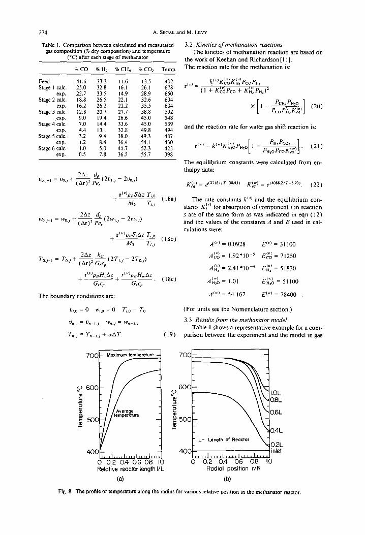
Fig. 8. The profile of temperature along the radius for various relative position in the methanator reactor,

Solar chemical heat pipe

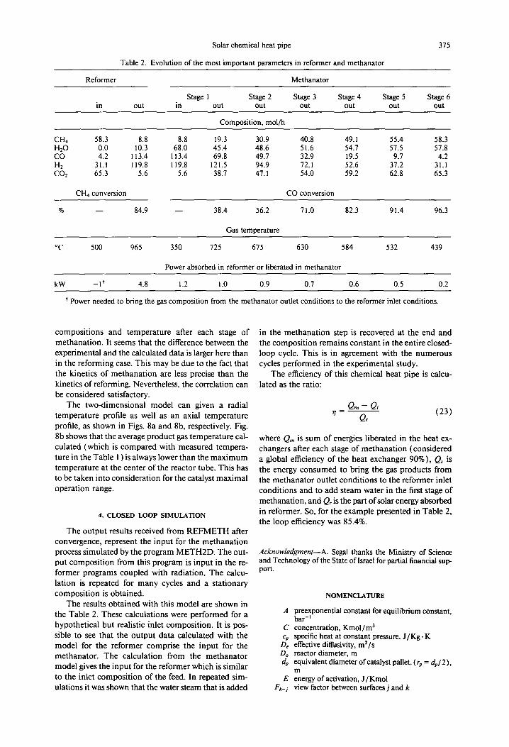
Table 2. Evolution of the most important parameters in reformer and methanator

375

Reformer Methanator

Stage 1 Stage 2 Stage 3 Stage 4 Stage 5 Stage 6 in out in out out out out out out

Composition, mol/h

CH4 58.3 8.8 8.8 19.3 30.9 40.8 49.1 55.4 58.3 H:O 0.0 10.3 68.0 45.4 48.6 51.6 54.7 57.5 57.8 CO 4.2 I 13.4 113.4 69.8 49.7 32.9 19.5 9.7 4.2 H2 31.1 119.8 119.8 121.5 94.9 72.1 52.6 37.2 31.1 CO2 65.3 5.6 5.6 38.7 47.1 54.0 59.2 62.8 65.3

CH4 conversion CO conversion

% - - 84.9 - - 38.4 56.2 71.0 82.3 91.4 96.3

Gas temperature

°C 500 965 350 725 675 630 584 532 439

Power absorbed in reformer or liberated in methanator

kW - I t 4.8 1.2 1.0 0.9 0.7 0.6 0.5 0.2

* Power needed to bring the gas composition from the methanator outlet conditions to the reformer inlet conditions.

composit ions and temperature after each stage of methanation. It seems that the difference between the experimental and the calculated data is larger here than in the reforming case. This may be due to the fact that the kinetics of methanat ion are less precise than the kinetics of reforming. Nevertheless, the correlation can be considered satisfactory.

The two-dimensional model can given a radial temperature profile as well as an axial temperature profile, as shown in Figs. 8a and 8b, respectively. Fig. 8b shows that the average product gas temperature cal- culated (which is compared with measured tempera- ture in the Table l ) is always lower than the max imum temperature at the center of the reactor tube. This has to be taken into consideration for the catalyst maximal operation range.

4. CLOSED LOOP SIMULATION

The output results received from R E F M E T H after convergence, represent the input for the methanation process simulated by the program METH2D. The out- put composit ion from this program is input in the re- former programs coupled with radiation. The calcu- lation is repeated for many cycles and a stationary composit ion is obtained.

The results obtained with this model are shown in the Table 2. These calculations were performed for a hypothetical but realistic inlet composition. It is pos- sible to see that the output data calculated with the model for the reformer comprise the input for the methanator. The calculation from the methanator model gives the input for the reformer which is similar to the inlet composit ion of the feed. In repeated sim- ulations it was shown that the water steam that is added

in the methanat ion step is recovered at the end and the composit ion remains constant in the entire closed- loop cycle. This is in agreement with the numerous cycles performed in the experimental study.

The efficiency of this chemical heat pipe is calcu- lated as the ratio:

Q ~ -- Qi (23) n Qr

where Qm is sum of energies liberated in the heat ex- changers after each stage of methanat ion (considered a global efficiency of the heat exchanger 90%), Qi is the energy consumed to bring the gas products from the methanator outlet conditions to the reformer inlet conditions and to add steam water in the first stage of methanation, and Q, is the part of solar energy absorbed in reformer. So, for the example presented in Table 2, the loop efficiency was 85.4%.

Acknowledgment--A. Segal thanks the Ministry of Science and Technology of the State oflsrael for partial financial sup- port.

NOMENCLATURE

A preexponential constant for equilibrium constant, bar - t

C concentration, Kmol/m 3 cp specific heat at constant pressure, J /Kg. K

/9, effective diffusivity, m2/s Do reactor diameter, m dp equivalent diameter of catalyst pallet, ( ro = do/2 ),

m E energy of activation, J /Kmol

F,_j view factor between surfacesj and k

376 A. SEGAL and M. LEVY

AH, H(') G k K

enthalpy change for a reaction, J /Kmol average gas mass velocity, Kg/m2s rate constant, Kmol / Kg catalyst, s equilibrium constant for a component absorption, bar-J

K~ equilibrium constant for a reaction, bar-" ke effective thermal conductivity, W / m . K L reactor length, m

MI molar rate refering to CO2 in feed, Kmol / s M3 molar rate refering to CO in feed, Kmol / s

P pressure, bar Q energy absorbed/liberated as heat, J • q heat flux, W / m 2

Per Peclet number ( u, dp/ De) R reactor radius, m r radial position, m r reaction rate, Kmol /Kg catalyst.s

S reactor cross section, m 2 T temperature, K

Tr, Thiele modulus, calculated after[ 8] U heat transfer coefficient between gas fluid and wall

surface, W / m 2 K u gas velocity, m/s x conversion in reforming reaction, Kmol CO2 con-

verted/Kmol CO2 in feed y conversion in reverse watergas shift reaction, Kmol

H20 formatted/Kmol CO2 in feed v conversion in methanation reaction, Kmol CH4

produced/Kmol CO in feed w conversion in water gas shift reaction, Kmol COz

formatted/Kmol CO in feed z position in length of reactor, m

c~k absorptivity of the surface k 6 reactor thickness, m

6kj Kronecker delta: = 1 for k = j ; =0 otherwise. On density of catalyst bed, Kg /m 3 a Stefan-Boltzmann constant, W / m 2 K 4

Subscripts and superscripts j , k

~7, IR arab

wall,i wall,o x Y 13

referring to surfaces j or k referring to visible or infra-red spectra referring to environmental medium referring to receiver wall interior or exterior referring to reforming reaction referring to reverse water gas shift reaction referring to methanation reaction

w referring to water gas shift reaction s referring to one of these reactions (s = x, y, v,

w) i where i = CH4, H20, CO, H2, CO2, referring

to one of these components

REFERENCES

I. M. Levy, R. Levitan, H. Rosin, and R. Rubin, Solar energy storage via a closed-loop chemical heat pipe, Solar Energy 50, 179 (1993).

2. R. Levitan, H. Rosin, and M. Levy, Chemical reactions in a solar furnace. Direct heating ofthe reactor in a tubular receiver, Solar Energy 42, 267 (1989).

3. A. Segal and E. Meirovitch, Storing concentrated sunlight in the chemical bond; A theoretical formulation, Heat Transfer 1990. Proc. of the Ninth Int. Heat Transf Con-

ference, Vol. 6, Jerusalem, Hemisphere Publishing Corp., New York, p. I 15 (1990).

4. A. Segal and E. Meirovitch, The computer modelling for a solar driven chemical reactor. Theoretical aspects, En- ergy and Environment into the 1990s, Proc. of the First World Renewable Energy Congress, Reading, UK, Per- gamonn Press, Oxford, p. 1197 (1990).

5. A. F. Emery, VIEW--version 5.5.3, Dept. of Mechanical Engineering, Univ. of Washington, Seattle (1986).

6. E. Meirovitch, A. Segal, and M. Levy, Theoretical mod- eling of a directly heated solar-driven chemical reactor, Solar Energy 45, 139 ( 1990 ).

7. R.F. Boehm, A review ofconvective loss data from solar central receivers, ASME J. Solar Energy Eng. 109, 101 (1987).

8. M. Levy, R. Levitan, E. Meirovitch, A. Segal, H. Rosin, and R. Rubin, Chemical reactions in a solar furnace. 2. Direct heating of a vertical reactor in an insulated receiver• Experiments and computer simulations, Solar Energy 48, 395 (1992).

9. A. Segal and M. Levy, Computer modelling of a solar chemical reactor, Solar Energy Materials 24, 725 (I 991 ).

10. J. M. Smith, Chemical engineering kinetics, McGraw- Hill, New York, p. 548 ( 1981 ).

1 I. D. Keehan and J. T. Richardson, Carbon monoxide rich methanation kinetics on supported rhodium and nickel catalysts, Report SAND88-7149, Sandia National Lab- oratories, Houston ( 1989 ).