Dimensioning Shared-per-Node Recirculating

Fiber Delay Line Buffers in an Optical Packet Switch

N. Akar1,∗

Electrical and Electronics Engineering Department

Bilkent University, Bilkent 06800, Ankara, Turkey

Y. Gunalay

Faculty of Economic and Administrative Sciences

Bahcesehir University, Besiktas 34353, Istanbul, Turkey

Abstract

Optical buffering based on fiber delay lines (FDL) has been proposed as a means for contention resolution

in an optical packet switch. In this article, we propose a queuing model for feedback-type shared-per-

node recirculating FDL optical buffers in asynchronous optical switching nodes. In this model, optical

packets are allowed to recirculate over FDLs as long as the total number of recirculations is less than a

pre-determined limit to meet signal loss requirements. Markov Modulated Poisson Process (MMPP)-based

overflow traffic models and fixed-point iterations are employed to provide an approximate analysis procedure

to obtain blocking probabilities as a function of various buffer parameters in the system when the packet

arrival process at the optical switch is Poisson. The proposed algorithm is numerically efficient and accurate

especially in a certain regime identified with relatively long and variably-sized FDLs, making it possible to

dimension optical buffers in next-generation optical packet switching systems.

Keywords: Optical packet switching, Optical burst switching, Markov modulated Poisson process,

Overflow models, Fiber delay lines

1. Introduction

One of the candidate transport mechanisms for next-generation Internet is based on the optical packet

switching paradigm that promises to provide efficient utilization of very high fiber capacities offered byWDM

technologies by means of switching at finer granularities. This is in contrast with the current state-of-the-

art optical circuit switching paradigm that provides point-to-point connectivity where bandwidth sharing

∗Corresponding authorEmail addresses: akar@ee.bilkent.edu.tr (N. Akar), yavuz.gunalay@bahcesehir.edu.tr (Y. Gunalay)

1The work of N. Akar is supported in part by the Science and Research Council of Turkey (Tubitak) under project no:EEEAG-111E106.

Preprint submitted to Elsevier July 3, 2013

at sub-wavelength levels is costly. The literature in this field comprises two key packet switching-based

paradigms: Optical Packet Switching (OPS) and Optical Burst Switching (OBS) [1],[2],[3],[4]. OBS does

not rely on optical header processing or optical buffers as in OPS but it is possible to deploy optical buffers

at OBS nodes to enhance burst blocking performance. Optical packets have fixed or variable sizes that are

integer multiples of a time unit, called slot, in synchronous switching [5]. On the other hand, optical packets

in asynchronous switching systems are of variable-length and therefore packet arrivals need not be aligned.

Using a retrial-queuing framework, we analytically study the performance of an asynchronous OPR (Optical

Packet Router), referring to an asynchronous OPS or OBS node, that uses FDLs (Fiber Delay Line) for

optical buffering.

Contention is said to occur when there are multiple optical packets on the same wavelength that are

simultaneously destined to the same output link. When the incoming packet’s wavelength is busy at the

destination link, then wavelength conversion can be used [6]. If all wavelengths are busy, then optical

buffering is one of the alternative means to resolve contention [3],[7]. Due to the lack of optical random

access memory with current technologies, FDLs are often used for optical buffering where an optical packet

finding all wavelengths occupied at the destination link is instead sent over a coil of fiber that provides the

packet with a deterministic delay with the potential of resolving contention at a later time. For different

architectures proposed for FDL buffering, we refer the reader to [3],[8],[9]. Optical buffers can be single-

stage or multi-stage, the latter having multiple blocks of delay lines cascaded together [10]. In a feed-forward

architecture, an output port of a switching element at a given stage is connected by an FDL to an input

port of a switching element at the next stage. In a feedback architecture, the output port of a switching

element at a given stage is connected to an input port of a switching element at the same stage [10]. A

packet that is sent over an FDL reserves the output in two different ways [4],[11]:

• If the output link is reserved prior to entering the buffer, this architecture is called Pre-Reservation

(PreRes).

• In the Post-Reservation (PostRes) scheme, the packet attempts to reserve the output link once it is

about to leave the FDL.

With PreRes reservation mechanism, a packet leaving the FDL buffer is guaranteed to find an idle wavelength

on the destination link whereas in the PostRes scheme, a packet may still find all wavelengths busy at its

destination link at the epoch of exit from the FDL. When such a situation arises, this packet will go through

multiple but limited number of FDL circulations. The advantage of PostRes buffers is the reduction in state

that is maintained at the node since the switch controller only needs to keep track of whether each wavelength

channel is busy or idle at a given time for PostRes. In contrast, the PreRes reservation mechanism requires

the switch controller to keep track of future channel occupancy information. PreRes schemes are generally

known to be more efficient in terms of performance since packets would not waste FDL resources in PreRes

2

if they would get blocked eventually. FDL buffers can be shared for all wavelength channels on a given link

in which case we have shared-per-link buffering. On the other hand, if FDLs are shared for all wavelength

channels for a given node, then we have the so-called shared-per-node FDL buffering in which case we have

performance benefits due to economy of sharing.

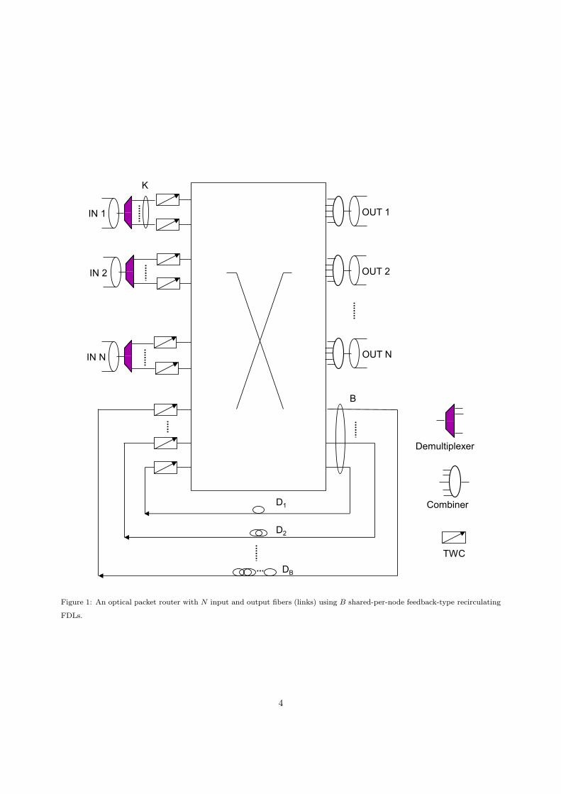
The scope of this article is on shared-per-node feedback-type recirculating FDL buffers using the PostRes

reservation model due to its relative implementation simplicity. For this purpose, we consider the OPR

architecture in Fig. 1 with N input and output links (or fibers) where each link comprises K wavelength

channels. This architecture is based on the tune-and-select (TAS) architecture with shared FDL buffers and

full range tuneable wavelength converters (TWC) described in [12]. We assume a shared pool of B FDLs

which can all be of the same length or variable-length delay lines can be used. To accommodate both cases,

we introduce an FDL spreading parameter α, 0 ≤ α < 1, and delay parameter D > 0. In our model, the ith

delay line introduces a delay of

Di = D(1− α) + (i − 1)2Dα

B − 1, i = 1, 2, . . . , B, if B > 1. (1)

In case B = 1, we have a single FDL with delay D. Based on the definition above, the minimum (maximum)

length delay line provides a delay of Dmin = D1 = D(1 − α) (Dmax = DB = D(1 + α)) and the average

delay of the delay lines is exactly D. Moreover, all the other delay lines are uniformly placed in between

the minimum and maximum delay line lengths. When α = 0, all delay lines are of the same length, i.e., of

length D. On the other hand, when α → 1, the delay line lengths tend to range between 0 and 2D. The

spreading parameter α can therefore be used to study the impact of fixed or variable-length delay lines.

The input signals in Fig. 1 are first wavelength de-multiplexed and the optical packets are converted to

the desired output wavelength using the TWCs in the tune stage. Subsequently, each signal is split up

to be sent to all output fibers and FDLs; but only one will be selected by switching on the corresponding

semiconductor optical amplifier (SOA) in the select stage. Finally, all selected signals destined to the same

fiber are combined. This architecture can be modified for the special case α = 0 for which we can use

B/W physical FDLs where each FDL accommodates W > 1 parallel WDM channels as in [12] and [13], as

opposed to using B separate physical FDLs. This modification can also be extended for the general α 6= 0

case by noting recent FDL buffering technologies that promise to achieve different time delays for different

wavelength channels on the same physical FDL [14].

We assume an exponentially distributed packet duration with mean set to unity which is equivalent to

saying that the time unit we use is the time it takes to transmit a packet with average size. We also assume

a symmetric Poisson packet arrival process with intensity λ(0) for each destination link. Thus, the total

arrival rate to the switch is Nλ(0). The system load is denoted by ρ = λ(0)/K. The assumptions of Poisson

call arrivals and exponentially distributed call-holding times have been successfully used for circuit-switched

networks handling call-oriented traffic. Although it is not clear at this point what type of traffic models

3

Demultiplexer

Combiner

TWC

K

OUT 1

OUT 2

OUT N

IN 2

IN N

IN 1

B

D1

D2

DB

Figure 1: An optical packet router with N input and output fibers (links) using B shared-per-node feedback-type recirculating

FDLs.

4

to be appropriate for use in next-generation OPS networks, we still employ in the current article the same

tele-traffic models from circuit-switching literature for gaining insight into the operation of optical buffers.

An arriving (fresh) optical packet which finds all K wavelength channels occupied at its destination

link is forwarded to the FDL pool comprising B delay lines. Otherwise, it is transmitted on one of the

idle wavelength channels randomly. For a packet directed to the FDL buffer, if all FDLs are busy at their

entrance points, then this packet is dropped. Otherwise, the packet is transmitted on one of the FDLs that

is idle at its entrance point. Motivated by the PostRes model, the FDL selection process is all random.

Once the packet completes its journey on the FDL, it becomes a retrial packet as opposed to a fresh packet.

A retrial packet again checks if one of the K wavelength channels at its destination link is idle and if so it

is randomly transmitted on one of them. If none of the channels is available and the total FDL circulation

count of this packet at this switch is less than M , then this packet is forwarded to one of the B FDLs again

randomly, upon availability. Otherwise, the retrial packet gets dropped. Based on the PostRes reservation

model, the switch controller only needs to keep track of the binary information on whether each wavelength

channel and each FDL is idle (at its entrance point) or not. Moreover, we note that void-filling based channel

scheduling is not supported with PostRes.

Our goal is to build a stochastic model that accurately captures the behavior of shared-per-node feedback-

type FDL optical buffers using the PostRes reservation scheme. Most of the existing work capitalizes on

shared-per-link buffers with K = 1 wavelength channel using the PreRes reservation model. An approximate

method is proposed in [15] for this particular case which employs an iterative procedure which is simple

to implement for Poisson arrivals and exponential packet lengths whereas the reference [16] relaxes the

assumptions on inter-arrival and service times of [15]. Again, for the same model, closed-form expressions

for loss probabilities and expected delays are obtained in [17] for certain sub-cases whereas an exact analysis

procedure for the general case of Markovian arrivals is recently proposed in [18] using the theory of feedback

fluid queues. For general N and K, and for PreRes shared buffering, an approximate model is proposed

in [10]. For K = 1 but feedback-type shared-per-link FDLs, a queuing model is presented in [19] for the

case of limited number of recirculations. A retrial queuing model for the case K > 1 and for feedback-type

shared-per-link FDLs is proposed in [20] but with probabilistic circulations. However, to meet signal loss

requirements, a limit is generally imposed on the maximum allowable number of FDL circulations [19]. In

[21], a renewal model has been proposed for analyzing OPRs with shared-per-node PreRes FDL buffers.

However, variable-length FDLs and recirculations are not employed in this work. This method is then used

in [22] to derive the end-to-end burst blocking probability in a network of OPRs using a two-moment based

approximative scheme. On the other hand, we use Markov Modulated Poisson Process (MMPP)-based

traffic models based on [23] (also used in [20]) for overflow traffic modeling that allows one to match three

moments in addition to the DC value of the power spectrum of the overflow traffic. In the current article,

we extend the work in [20] in three directions:

5

• A more efficient FDL sharing scheme, namely shared-per-node FDL buffering, as opposed to shared-

per-link FDL buffering, is employed in the current study.

• In the current study, an optical packet can travel over an FDL at most M ≥ 1 times as opposed to

the less realistic probabilistic recirculation scheme of [20].

• We allow varying FDL lengths using the spreading parameter α > 0 as opposed to fixed-length FDLs

proposed in [20], which will be shown later to have significant benefits in terms of blocking performance

and amenability to analysis.

The motivation behind the introduction of a queuing model for FDL buffers is the need to assess if

optical packet-switched networks can be operated at reasonably high levels of utilization using feedback-type

recirculating FDLs. By simulations, we specify a range of D and α values for which the system performance

is relatively improved and also our proposed queuing model works acceptably well. Although the queuing

model does not take into consideration the particular values of D and α, it is capable of studying the impact

of other FDL parameters on blocking performance such as the FDL buffer size B, recirculation count M ,

number of wavelength channels K, and number of fibers N . FDLs need to be as short as possible since they

increase the delays in the network and the physical size of the buffer. However, statistical multiplexing gains

will be reduced with shorter FDLs since then a retrying packet will more likely see an all-occupied system

again. Moreover, increased number of FDLs used in the system lead to increased hardware complexity and

it is also important to minimize this number without sacrificing from performance. Recirculations are also

intuitively useful since they allow multiple opportunities for reserving a channel at the destination link.

However, recirculations introduce signal losses and additional delays and they should be kept at a minimum.

Simulations always provide an answer but using simulations for dimensioning purposes especially in a regime

of low loss probabilities is a tedious task. The retrial-queuing model we introduce in this paper can help

fill this gap so as to be used for engineering and dimensioning purposes in the context of shared-per-node

feedback-type recirculating FDL buffers.

The remainder of this article is organized as follows. In Section 2, we present an overview of the MMPP

and two-state MMPP construction that is crucial for the development of the paper. Section 3 presents the

queuing model we propose for feedback-type FDL buffers. In Section 4, we provide numerical examples for

validating the accuracy of this approach as well as the use of these models for engineering and dimensioning

purposes. Finally, we conclude.

2. Markov Modulated Poisson Process

The following is based on [24]. An MMPP is a point process whose intensity depends on the state of a

background process that is an irreducible finite-state continuous-time Markov chain. Let us assume m > 0

6

states for the background process. The MMPP is characterized by the infinitesimal generator Q of the

underlying Markov chain and by Λ, an m×m diagonal matrix with diagonal elements λ1, λ2, . . . , λm, i.e.,

Λ = diag(λ1, λ2, . . . , λm). In this case, we simply say the MMPP is characterized with the matrix pair

(Q,Λ). The operation of the MMPP is as follows. When the background process is in state i, the MMPP is

said to be in phase i and arrivals occur according to a Poisson process with rate λi. Let π be the steady-state

vector of Q, i.e., πQ = 0, πe = 1, where e is a column vector of ones of appropriate size. The rth non-central

moment of the arrival rate of the MMPP characterized with the pair (Q,Λ) is denoted by µr and is given

in [24] as µr = πΛre, r ≥ 1.

As opposed to renewal processes, successive inter-arrival times are correlated for MMPPs. This feature

of MMPP as well as its amenability to analysis has attracted researchers in the field of telecommunication

network traffic modeling. As one of the classical examples, a superposition of packetized voice sources

with silence detection is modeled as a two-state MMPP so as to analytically study the performance of a

voice multiplexer [25]. The reference [26] proposes an MMPP-based model that mimics the real hierarchical

behavior of the packet generation process by Internet users. An MMPP model is provided for multimedia

traffic in [27]. An Interrupted Poisson Process (IPP) is a two-state MMPP for which one of the two Poisson

intensities is zero which amounts to interrupting the arrival process in that particular state of the background

process. The most relevant application example to this paper is the use of MMPPs and in particular IPPs,

in modeling overflow traffic in circuit-switched networks [28],[23].

In most cases, using MMPPs with large state spaces are either computationally infeasible or impractical.

Most of the existing research concentrates on two-state MMPP modeling due to its versatility [25]. In this

article, we employ a technique from Heffes [29] that approximates a multi-state MMPP with one with two

states. The approach of [29] matches the first three non-central moments of the instantaneous arrival rate

of the MMPP and in addition an appropriately defined time constant for the process, which is defined in

terms of the integral of the covariance function of the instantaneous arrival rate of the MMPP. Note that the

above-mentioned integral amounts to the DC value of the associated power spectrum which is very critical

as far as queuing performance is concerned [30]. Let the original multi-state MMPP be characterized with

the matrix pair (Q(m),Λ(m)) with m > 2 states. Let the two-state approximative MMPP be characterized

with the pair (Q(2),Λ(2)). Also let

Q(2) =

−σ1 σ1

σ2 −σ2

,Λ(2) =

λ1 0

0 λ2

.

Let π(m) denote the stationary vector of the modulating Markov chain of the original MMPP (Q(m),Λ(m))

such that π(m)Q(m) = 0, π(m)e = 1. Also let µr denote the rth non-central moment of the arrival rate of

the MMPP (Q(m),Λ(m)) and v denote its variance that is given by v = µ2 − µ21. The time constant τc of

7

the original MMPP is expressed as

τc =1

v

∫∞

0

r(t)dt, (2)

where r(t) is the covariance function of the arrival rate. The reference [23] provides an expression for τc

that is easy to obtain:

τc =1

v[πΛ(m)(eπ(m) −Q(m))−1Λ(m)e− µ2

1].

Heffes [29] proposes to choose the parameters of the approximating two-state MMPP as follows:

σ1 =1

τc(1 + η), σ2 =

η

τc(1 + η), λ1 = µ1 +

√

v/η, λ2 = µ1 −√vη,

where

δ =µ3 − 3µ1v − µ3

1

v3/2, η = 1 +

δ

2(δ −

√

4 + δ2).

The above choices are shown in [29] to match the first three non-central moments as well as the time

constant defined in (2). When this method is used for MMPP model reduction, we will say the pair

(Qm),Λ(m)) is reduced to the matrix pair (Q(2),Λ(2)) using Heffes’ method or mathematically, (Q(2),Λ(2)) =

fH(Q(m),Λ(m)) where the function fH represents Heffes’ method.

The superposition of independent MMPPs is also an MMPP. Consider the superposition of n not-

necessarily identical two-state MMPPs. The state-space, in lexicographic order, can be described by Kro-

necker calculus [31]. Given A = {Aij}, a p× p matrix, and a q × q matrix B, the Kronecker product of the

matrices A and B is denoted by A ⊗ B and is given as a matrix with block elements {AijB}. Therefore,

the size of the square matrix A⊗B is pq. The Kronecker sum of the matrices A and B is denoted by A⊕B

and is given by A ⊗ Iq + Ip ⊗ B, where Ik denotes an identity matrix with size k. With this notation, the

superposition of n independent two-state MMPPs characterized with (Qi,Λi), 1 ≤ i ≤ n can be represented

by the superposition MMPP (Q,Λ) [23] where

Q = Q1 ⊕Q2 ⊕ · · · ⊕Qn

= Q1 ⊗ I2 ⊗ · · · ⊗ I2 + I2 ⊗Q2 ⊗ I2 ⊗ · · · ⊗ I2 + · · · + I2 ⊗ I2 ⊗ · · · ⊗ I2 ⊗Qn

Λ = Λ1 ⊕ Λ1 ⊕ · · · ⊕ Λn

The superposition can be handled only with n+ 1 states instead of 2n states when the individual two-state

MMPPs are identically distributed. In this case, we have

Qi =

−σ1 σ1

σ2 −σ2

,Λi =

λ1 0

0 λ2

, 1 ≤ i ≤ n,

8

and the superposition MMPP can be represented by (Q,Λ) where

Q =

−nσ1 nσ1

σ2 −(σ2 + (n− 1)σ1). . .

. . .. . . σ1

nσ2 −nσ2

,Λ =

nλ1

(n− 1)λ1 + λ2

. . .

nλ2

,

since in this case, the state i, 0 ≤ i ≤ n, keeps track of the number of individual MMPPs which are in their

first state and we do not have to keep track of the states of individual MMPPs.

3. Analytical Model

Since there is symmetry among the output links, we concentrate on one single tagged output link that

comprises K wavelength channels. This tagged link is associated with the so-called fiber process {X(t) : t ≥0, 0 ≤ X(t) ≤ K} which keeps track of the number of busy wavelength channels on the tagged link at time t.

Recall that the fresh traffic destined to the tagged link is Poisson with intensity λ(0). Let the retrial process

{Yi(t) : t ≥ 0, 1 ≤ i ≤ M} denote the arrival process to the tagged link stemming from optical packets that

have already traversed FDLs i times. Note that {Yi(t)} is a count process that counts up each time a packet

(destined for the tagged link) leaves the FDL buffer and this amounts to the ith circulation of the packet

over the FDLs. Equivalently, the retrial process {Yi(t)} has overflown from the tagged link i times and the

packet has found an idle FDL at the epoch of overflows. Provided that FDL delays are sufficiently long,

i.e., D >> 1 and the spreading parameter α is relatively large, i.e., α >> 0, we conjecture that the retrial

process {Yi(t)} can well be approximated with a Poisson process with intensity λ(i), 1 ≤ i ≤ M . In this

operating regime, i.e., D >> 1, α >> 0, the processes {(Y1(t), . . . , YM (t), X(t))} are also approximated as

independent processes. We note that the analytical model we propose is based on these two approximations

which are valid in the above-mentioned operating regime and therefore does not take into consideration the

particular choices of the parameters D and α. We will later show the validity of these approximations by

simulations in Section 4.

Furthermore, we define the overflow process {Zj(t) : t ≥ 0, 1 ≤ j ≤ M} that represents the overflow

process of the tagged link corresponding to packets that have overflown from the tagged link j times and are

in the process of searching for an idle FDL. Obviously, when B → ∞, for 1 ≤ j ≤ M , {Zj(t)} and {Yj(t)}correspond to the same count process since in this case an overflown packet will always get to find an idle

FDL. We do not know λ(i), 1 ≤ i ≤ M , yet but we will attempt to find them using an iterative procedure

as described below.

Let us assume the quantities λ(i), 1 ≤ i ≤ M , are now available. Then the process {X(t)} is a birth-death

process with constant birth rate λ =∑M

i=0 λ(i) and death rate k when X(t) = k, 1 ≤ k ≤ K. Let P denote

9

the generator of this process. Let x denote the stationary vector of P such that xP = 0, xe = 1, and partition

x = (x0, x1, . . . , xK). As shown in the classical circuit switching literature [23], the overflow process {Zj(t)}is not Poisson since the inter-event times associated with the process {Zj(t)} are highly correlated due to

the way overflows occur. Therefore, there is a need for more elaborate modeling of the overflow traffic taking

into consideration such correlation effects. Actually, {Zj(t)} can exactly be modeled through a (K+1)-state

MMPP characterized with the matrix pair (P,Λj), 1 ≤ j ≤ M , where Λj is an all-zeros matrix except for its

single south-east corner entry set to λ(j−1). To cope with the state-space explosion problem, we use Heffes’

method described in the previous section to reduce the (K + 1)-state MMPP to a two-state MMPP. With

this method in place, we suggest that the process {Zj(t)}, 0 ≤ j ≤ M , is to be approximated by a two-state

MMPP characterized with the pair (Pj , Cj) defined through (Pj , Cj) = fH(P,Λj) for 1 ≤ j ≤ M . Let us

then write

Pj =

−κ

(j)1 κ

(j)1

κ(j)2 −κ

(j)2

, Cj =

c(j)1 0

0 c(j)2

, 1 ≤ j ≤ M . (3)

In this particular scenario, due to the way Λj is structured, the two-state MMPP (Pj , Cj) is actually an

IPP, i.e., c(j)1 = 0, as shown in [23] but we keep the notation more general for the sake of convenience.

Note that {Zj(t)} is the contribution of overflow traffic due to the single tagged fiber only. Let {Zj(t); 1 ≤j ≤ M} be the overflow process for the entire OPR corresponding to packets that have overflown from any

one of the N fiber links j times and which are in the process of finding an idle FDL. The overflow process

{Zj(t)} is then called the jth parcel using the terminology of [23]. Moreover, this process can approximately

be represented by a two-state MMPP characterized with the matrix pair (Qj , Rj) [23]. Since {Zj(t)} is

obtained through the superposition of N individual overflow processes, this two-state MMPP model can be

obtained by using Heffes’ model reduction method [29] similar to the approach in [23]: (Qj , Rj) =

fH

(

−Nκ(j)1 Nκ

(j)1

κ(j)2 −(κ

(j)2 + (N − 1)κ

(j)1 )

. . .

. . .. . . κ

(j)1

Nκ(j)2 −Nκ

(j)2

,

Nc(j)1

(N − 1)c(j)1 + c

(j)2

. . .

Nc(j)2

)

.

(4)

Let ηj denote the mean arrival rate for the jth parcel which is the mean rate of the MMPP (Qj , Rj).

The superposition of M independent MMPPs parameterized by (Qj , Rj), 1 ≤ j ≤ M can be represented by

the MMPP (Q,R) with

Q = Q1 ⊕Q2 ⊕ · · · ⊕QM , R = R1 ⊕R2 ⊕ · · · ⊕RM . (5)

The MMPP (Q,R) is offered to B FDLs of varying length. An accepted packet into the buffer occupies the

entrance point of the FDL for a duration which is equal to the packet transmission time. This observation

leads to a MMPP/M/B/B queuing system on the state space {(l, l′), 1 ≤ l ≤ B, 1 ≤ l′ ≤ 2M} [23] where

10

l corresponds to the number of FDLs that are occupied at their entrance points and l′ represents the

state of the incoming MMPP with infinitesimal generator Q. As in [23], the infinitesimal generator of the

MMPP/M/B/B system is given by the following matrix

V =

Q−R R

I Q−R − I R

2 I Q−R− 2I R

. . .. . .

. . .

BI Q −BI

, (6)

where I denotes an identity matrix of size 2M . The performance measures of the system can be calculated

by studying the stationary vector π = (π0, π1, . . . , πB) of V which satisfies

πV = 0, πe = 1. (7)

It is clear that V has 2MB states but one can utilize the block-tridiagonal structure of V to obtain π

with a computational complexity that is linear in B; see for example the block-tridiagonal LU factorization

algorithm [32]. When a packet belonging to parcel j finds all the B FDLs occupied, then blocking occurs

due to the lack of an idle FDL. In this case, the blocking probability for parcel j, denoted by γj , is given by

γj =πBVje

ηj, (8)

where

Vj = 0⊕ 0⊕ · · · ⊕ Rj︸︷︷︸

j th position

⊕ 0⊕ · · · ⊕ 0. (9)

Since {Yj(t)} is assumed to be Poisson and is obtained from {Zj(t)} by choosing those packets that get to

find an idle FDL, we have

λ(j) =ηj(1 − γj)

N, 1 ≤ j ≤ M. (10)

In the methodology described above, once we know the arrival intensities λ(i), 1 ≤ i ≤ M , one can obtain

the pair (Q,R) that characterizes the MMPP traffic offered to the B FDL buffers. On the other hand, given

the pair (Q,R), one can obtain λ(i), 1 ≤ i ≤ M , as in (10). Therefore, the overall problem can be solved by

means of a fixed point procedure described in Table 1.

Upon convergence of the fixed point procedure, we can find the overall blocking probability PB based on

the expression below:

PB =xKλ(M)N +

∑Mj=1 πBVje

Nλ(0)(11)

The term xKλ(M) in the numerator above amounts to the rate of packets that are blocked due to the

lack of an idle wavelength channel at the tagged link once the recirculation limit is reached. This term

11

Table 1: Algorithm to find PB given λ(0), K, N , B, and M .

1. Set λ(i) = 0, 1 ≤ i ≤ M .

2. Form the generator P for the fiber process which is of birth-and-death

type. Also form the matrices Λj , 1 ≤ j ≤ M .

3. For 1 ≤ j ≤ M , using Heffes’ method, reduce the (K + 1)-state MMPP

(P,Λj) to the two-state MMPP (Pj , Cj) as in (3).

4. For 1 ≤ j ≤ M , obtain the MMPP (Qj , Rj) (parcel j) as in (4).

5. Calculate ηj which is the mean arrival rate of the MMPP (Qj, Rj) that

is written as ηj = yjRje where yj is the stationary vector of Qj , i.e.,

yjQj = 0, yje = 1.

6. Obtain the MMPP (Q,R) based on (5).

7. Form the generator V for the buffer process as in (6) and calculate

its stationary vector π satisfying πV = 0, πe = 1. Also partition π =

(π0, π1, . . . , πB).

8. Calculate the parcel-j blocking probability γj as in (8).

9. For 1 ≤ j ≤ M , write λ(j) as in (10).

10. If the successive values for λ(j), 1 ≤ j ≤ M are sufficiently close, conver-

gence is reached. Upon convergence, write the loss probability PB as in

(11) and exit. Otherwise, go to Step 2.

is multiplied with the factor N since there are N such links. On the other hand, the second term in the

numerator represents the rate of packets that are blocked due to the lack of an idle FDL at one of the retrial

attempts. The denominator gives the rate of fresh packets into the OPR and the ratio gives the packet

blocking probability. Similarly, one can find the distribution of the number of FDL recirculations. For this

purpose, let H denote the number of retrials required for a successful packet. It is easy to show that

P (H = h) =λ(h)(1− xK)

λ(0)(1 − PB), 0 ≤ h ≤ M. (12)

4. Numerical Results

For the fixed point procedure, let λk denote the vector of retrial rates λ(i), 1 ≤ i ≤ M , at the end of

the kth iteration. We stop the iterations when |λk − λk−1|2/|λk|2 < ε for some tolerance parameter ε

which is set to 0.00001 for the numerical examples of this article. We ran the fixed point procedure for all

combinations involving N ∈ {4, 8, 16},K ∈ {8, 16, 32}, B ∈ {8, 16, 32},M ∈ {1, 2, 3} and ρ ∈ {0.5, 0.7, 0.9}.The iterations converged rapidly in all cases; the minimum (maximum) number of iterations required was 4

12

(27) for this experiment. The number of required iterations appear to increase with increased B and ρ but

with decreased N values but convergence was acceptably fast in all cases we tested.

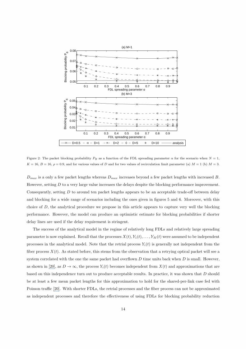
We first validate the analytical method proposed in the previous section by simulations in figures 2-6.

For this purpose, we first fix N = 1, K = 16, B = 16, ρ = 0.9 and we plot the blocking probability PB

obtained using simulations as a function of the FDL spreading parameter α for various values of D and for

two values of the recirculation limit parameter M in Fig. 2. Fig. 3 addresses the same scenario but with

load ρ reduced to 0.75 while all other parameters are fixed. We further increase the number of fibers N with

ρ fixed at 0.75 to 8 in a new simulation scenario whose results are depicted similarly in Fig. 4. The results

obtained via the analytical model are also depicted in figures 2-4. It is clear that the blocking probability

PB decreases as D increases in all scenarios for fixed α. This stems from the observation that for low values

of D, a retrying optical packet will see a system occupancy positively correlated with the one the same

packet had attempted to join but failed D time units back. Similar observations were made in [11] and

[20]. Using FDLs of varying lengths is generally peculiar to PreRes schemes but it is clear from figures 2-4

that such different length FDLs also reduce blocking probabilities in PostRes schemes. The packet blocking

probability PB first decreases with increasing FDL spreading parameter α but beyond a certain value of α,

it tends to slightly increase as α → 1 for all the three scenarios we tested. This latter behavior is more

evident for relatively low values of D and M . To explain this phenomenon, as α → 1, some of the delay lines

will induce very small delays compared to the average packet length and consequently retrying packets using

such small FDLs will likely get blocked. However, with a proper choice of the FDL spreading parameter α,

for example α = 0.8, such behavior can be avoided. Throughout the rest of the paper, we set α = 0.8.

In the second simulation example, we fix N = 8, K = 16, and study the accuracy of the analytical model

in terms of B, M , and ρ. For this purpose, we plot the blocking probability PB for various values of D in

Fig. 5 obtained by simulations (recall α = 0.8 used throughout all simulations) as a function of the FDL

size B for four different scenarios corresponding to ρ = 0.7, 0.9 and M = 1, 5. This plot also presents the

results of the analytical model. We observe that for a given scenario, there is a certain value of D, say

Dmax, beyond which there will be no significant performance improvement in terms of blocking probability.

However, Dmax turns out to depend on the presented scenario. Based on the results provided in Fig. 5,

when the average delay length D is chosen so that it is larger than Dmax, then the analytical model captures

very well the blocking performance with respect to the FDL size B.

It is also crucial to choose an absolute value for D to use in the OPR. For this purpose, we design the

following simulation experiment. Fixing M = 5, K = 16, and for given N and B, for two values of desired

blocking probability PB = 0.01, 0.001, we find λ(0) that meets the blocking probability requirement using

the analytical model. We then simulate the corresponding OPR offered with Poisson traffic with intensity

λ(0) for various values of D. The results of this simulation experiment are presented in Fig. 6. We observe

that irrespective of the choice of the switch size N , Dmax turns out to depend on B; for low values of B,

13

0.1 0.2 0.3 0.4 0.5 0.6 0.7 0.8 0.9

0.05

0.06

0.07

0.08

FDL spreading parameter α

(a) M=1

Blo

ckin

g pr

obab

ility

PB

0.1 0.2 0.3 0.4 0.5 0.6 0.7 0.8 0.9

0.01

0.02

0.03

0.04

0.05

(b) M=3

FDL spreading parameter α

Blo

ckin

g pr

obab

ility

PB

D=0.5 D=1 D=2 D=5 D=10 analysis

Figure 2: The packet blocking probability PB as a function of the FDL spreading parameter α for the scenario when N = 1,

K = 16, B = 16, ρ = 0.9, and for various values of D and for two values of recirculation limit parameter (a) M = 1 (b) M = 3.

Dmax is a only a few packet lengths whereas Dmax increases beyond a few packet lengths with increased B.

However, setting D to a very large value increases the delays despite the blocking performance improvement.

Consequently, setting D to around ten packet lengths appears to be an acceptable trade-off between delay

and blocking for a wide range of scenarios including the ones given in figures 5 and 6. Moreover, with this

choice of D, the analytical procedure we propose in this article appears to capture very well the blocking

performance. However, the model can produce an optimistic estimate for blocking probabilities if shorter

delay lines are used if the delay requirement is stringent.

The success of the analytical model in the regime of relatively long FDLs and relatively large spreading

parameter is now explained. Recall that the processesX(t), Y1(t), . . . , YM (t) were assumed to be independent

processes in the analytical model. Note that the retrial process Yi(t) is generally not independent from the

fiber process X(t). As stated before, this stems from the observation that a retrying optical packet will see a

system correlated with the one the same packet had overflown D time units back when D is small. However,

as shown in [20], as D → ∞, the process Yi(t) becomes independent from X(t) and approximations that are

based on this independence turn out to produce acceptable results. In practice, it was shown that D should

be at least a few mean packet lengths for this approximation to hold for the shared-per-link case fed with

Poisson traffic [20]. With shorter FDLs, the retrial processes and the fiber process can not be approximated

as independent processes and therefore the effectiveness of using FDLs for blocking probability reduction

14

0 0.1 0.2 0.3 0.4 0.5 0.6 0.7 0.8 0.90

2

4

6

8

10x 10

−3

FDL spreading parameter α

Blo

ckin

g pr

obab

ility

PB

(b) M=3

0 0.1 0.2 0.3 0.4 0.5 0.6 0.7 0.8 0.90.005

0.01

0.015

0.02

0.025

0.03

FDL spreading parameter α

(a) M=1

Blo

ckin

g pr

obab

ility

PB

D=0.5 D=1 D=2 D=5 D=10 analysis

Figure 3: The packet blocking probability PB as a function of the FDL spreading parameter α for the scenario when N = 1,

K = 16, B = 16, ρ = 0.75, and for various values of D and for two values of recirculation limit parameter (a) M = 1 (b)

M = 3.

is relatively limited. For the spreading parameter effect on performance, let us assume α → 0 first. In

this case, it is obvious that Yi(t) and Yj(t), i 6= j are not independent. To see this, let us assume severe

congestion at the tagged fiber at around time t0. There will be retrial traffic that will retry all together

at t0 +D. Since the instantaneous rate of this retrial process will be high, the system will continue to be

congested at time t0 + D leading to an increase of instantaneous rate of retrial traffic at t0 + 2D, and so

on. This shows that X(t0), Yi(t0 + iD), 1 ≤ i ≤ M are not independent. In order to break this dependence,

we introduce in this paper the spreading parameter α and random FDL selection policy. Using figures 2-4,

we show the impact of the choice of α on the independence assumption. Therefore, use of long average

FDL delays D and relatively large spreading parameter α (for example α = 0.8) is not only effective in

improving blocking performance but also in this regime, an analytical model can be built on the basis of the

independence assumption of the processes X(t), Y1(t), . . . , YM (t).

For the remainder of this article, we provide results obtained only using the analytical model assuming

that the average FDL size parameter D is set to a value exceeding ten packet lengths as motivated before.

We now define the achievable throughput T as the maximum load the OPR can support under a blocking

probability constraint PB. We fix N = 8 and plot T associated with the blocking constraint PB < 0.001 as

a function of the FDL size B for various values of M in Fig. 7 for two different choices of K: (a) K = 8

15

0 0.1 0.2 0.3 0.4 0.5 0.6 0.7 0.8 0.90.01

0.015

0.02

0.025

0.03

FDL spreading parameter α

Blo

ckin

g pr

obab

ility

PB

(a) M=1

0 0.1 0.2 0.3 0.4 0.5 0.6 0.7 0.8 0.90.005

0.01

0.015

0.02

0.025(b) M=3

FDL spreading parameter α

Blo

ckin

g pr

obab

ility

PB

D=0.5 D=1 D=2 D=5 D=10 analysis

Figure 4: The packet blocking probability PB as a function of the FDL spreading parameter α for the scenario when N = 8,

K = 16, B = 16, ρ = 0.75, and for various values of D and for two values of recirculation limit parameter (a) M = 1 (b)

M = 3.

(b) K = 16. The results are obtained only through the proposed analytical model. Note that the B = 0

case does not employ FDLs and the corresponding throughput is obtained using the Erlang-B formula for

K servers. We observe that there is a certain value of B, say Bmax, beyond which the throughput T can

not further be improved. The quantity Bmax however increases with increasing M and also with increasing

K. When small FDL sizes are used (B → 0), there is limited gain in using multiple circulations M > 1.

However, one can benefit from multiple circulations for larger FDL sizes. Consider the basic case of using

one circulation only and using Bmax FDLs. In this case, the throughput is increased by 88.5% and 52.6%,

associated with the cases K = 8 and K = 16, respectively, compared with the bufferless scenario. Even with

such basic schemes, the throughput can substantially be improved.

The final numerical experiment we present is on the provisioning of the FDL size B. Again, for a given

blocking probability PB = 0.001, and for given N,M,K, and B, we iteratively calculate T but also find the

value of B, namely Bmax, beyond which T does not change significantly. In this example, Bmax is found

so that the difference in T values corresponding to FDL sizes Bmax and Bmax + 1 is less than 0.001. Once

the targeted FDL size Bmax is found, the maximum throughput achievable by using an FDL size of Bmax

is called Tmax. The FDL size requirement Bmax and the corresponding maximum achievable throughput

Tmax are plotted in Fig. 8. Our observations are:

16

10 20 30 40 50 600.015

0.02

0.025

0.03

0.035

0.04

0.045

FDL Size B

Blo

ckin

g P

roba

bilit

y P

B

(a) ρ=0.7, M=1

D=2D=5D=10analysis

10 20 30 40 50 6010

−6

10−4

10−2

FDL Size B

Blo

ckin

g P

roba

bilit

y P

B

(b) ρ=0.7, M=5

D=2D=5D=10analysis

20 40 60 80 100

0.08

0.09

0.1

0.11

0.12

0.13

FDL Size B

Blo

ckin

g P

roba

bilit

y P

B

(c) ρ=0.9, M=1

D=2D=5D=10analysis

20 40 60 80 100 120 14010

−2

10−1

FDL Size B

Blo

ckin

g P

roba

bilit

y P

B

(d) ρ=0.9, M=5

D=2D=5D=10analysis

Figure 5: The packet blocking probability PB as a function of the FDL delay parameter B for various values of D for the

scenario when α = 0.8, N = 8, K = 16: (a) ρ = 0.7,M = 1 (b) ρ = 0.7,M = 1 (c) ρ = 0.9,M = 1 (d) ρ = 0.9,M = 5.

• The FDL size requirement Bmax changes almost linearly with K and M .

• The FDL size requirement Bmax increases with increased switch size N . However, the maximum

achievable throughput Tmax obtained using Bmax FDLs does not change much with increased switch

size N .

• Most of the throughput gains stem from one or two circulations with incremental changes with further

number of recirculations.

5. Conclusion

We propose an MMPP-based queuing model along with fixed-point iterations to accurately evaluate the

performance of feedback-type shared-per-node recirculating FDL buffers. Simulation results show that the

proposed model allows us to accurately estimate the packet blocking performance in a certain regime of

long FDL delay D along with the employment of a relatively large spreading parameter α. Benefits of using

17

5 10 15 20 25 30

10−3

10−2

FDL Delay D

Blo

ckin

g P

roba

bilit

y P

B

N=4, B=4

N=4, B=16

N=8, B=4

N=8, B=16

PB=0.01

PB=0.001

Figure 6: The packet blocking probability PB as a function of the FDL delay parameter D for various values of N and B when

M = 5, K = 16 and for two values of desired blocking probability PB = 0.01, 0.001.

variable length FDLs are justified in a feedback architecture using the PostRes reservation scheme, which

to the best of our knowledge, is novel. Moreover, the retrial-queuing model proposed in this article can

effectively be used in dimensioning feedback-type shared-per-node recirculating FDL optical buffers.

References

[1] P. Gambini, M. Renaud, C. Guillemot, F. Callegati, I. Andonovic, B. Bostica, D. Chiaroni, G. Corazza, S. L. Danielsen,

P. Gravey, P. B. Hansen, M. Henry, C. Janz, A. Kloch, R. Krahenbuhl, C. Raffaelli, M. Schilling, A. Talneau, L. Zucchelli,

Transparent optical packet switching: network architecture and demonstrators in the KEOPS project, IEEE J. Select.

Areas Commun. 16 (1998) 1245–1259.

[2] C. Qiao, M. Yoo, Optical burst switching (OBS) - a new paradigm for an optical Internet, Jour. High Speed Networks

(JHSN) 8 (1999) 69–84.

[3] L. Xu, H. Perros, G. Rouskas, Techniques for optical packet switching and optical burst switching, IEEE Communications

Magazine 39 (2001) 136 –142.

[4] T. Battestilli, H. Perros, An introduction to optical burst switching, Communications Magazine, IEEE 41 (2003) S10 –

S15.

[5] F. Callegati, W. Cerroni, G. Corazza, C. Develder, M. Pickavet, P. Demeester, Scheduling algorithms for a slotted packet

switch with either fixed or variable length packets, Photonic Network Communications 8 (2004) 163–176.

[6] R. Barry, P. Humblet, Models of blocking probability in all-optical networks with and without wavelength changers, IEEE

Journal on Selected Areas in Communications 14 (1996) 858–867.

[7] I. Chlamtac, A. Fumagalli, L. Kazovsky, P. Melman, W. Nelson, P. Poggiolini, M. Cerisola, A. Choudhury, T. Fong,

18

0 10 20 30 40 50 60

0.3

0.4

0.5

0.6

0.7

0.8

0.9

FDL Size B

Thr

ough

put T

(a) N=8, K=8

M=1 M=2 M=3 M=4 M=5 M=6

0 10 20 30 40 50 60 70 80 900.4

0.5

0.6

0.7

0.8

0.9

(b) N=8, K=16

FDL Size B

Thr

ough

put T

Figure 7: The achievable throughput T under a desired blocking probability PB = 0.001 as a function of the FDL size B for

various values of M for N = 8 and for two different values of K: (a) K = 8 (b) K = 16.

19

5 10 15 20 25 300.2

0.4

0.6

0.8

1

Number of wavelengths per link K

Tm

ax

(b) Tmax

(N=8)

5 10 15 20 25 300

50

100

150

200

250

300

(c) Bmax

(N=32)

Number of wavelengths per link K

Bm

ax

5 10 15 20 25 300.2

0.4

0.6

0.8

1

Number of wavelengths per link K

Tm

ax

(d) Tmax

(N=32)

5 10 15 20 25 300

20

40

60

80

100

(a) Bmax

(N=8)

Number of wavelengths per link K

Bm

ax

M=1

M=2

M=3

M=1

M=2

M=3

M=1

M=2

M=3

M=1

M=2

M=3

Figure 8: The FDL size requirement Bmax and the corresponding maximum achievable throughput Tmax as a function of K

for three values of M and for two values of N .

20

R. Hofmeister, C.-L. Lu, A. Mekkittikul, I. Sabido, D.J.M., C.-J. Suh, E. Wong, CORD: contention resolution by delay

lines, IEEE Journal on Selected Areas in Communications 14 (1996) 1014–1029.

[8] D. Hunter, M. Chia, I. Andonovic, Buffering in optical packet switches, Journal of Lightwave Technology 16 (1998) 2081

–2094.

[9] W. D. Zhong, R. S. Tucker, Wavelength routing-based photonic packet buffers and their applications in photonic packet

switching systems, Journal of Lightwave Technology 16 (1998) 1737 –1745.

[10] T. Zhang, K. Lu, J. Jue, Shared fiber delay line buffers in asynchronous optical packet switches, Selected Areas in

Communications, IEEE Journal on 24 (2006) 118–127.

[11] C. M. Gauger, Dimensioning of FDL buffers for optical burst switching nodes, in: Proceedings of the 6th IFIP Working

Conference on Optical Network Design and Modelling (ONDM 2002).

[12] C. Gauger, H. Buchta, E. Patzak, Integrated evaluation of performance and technology-throughput of optical burst

switching nodes under dynamic traffic, Lightwave Technology, Journal of 26 (2008) 1969–1979.

[13] C. McArdle, D. Tafani, L. Barry, A. Holohan, T. Curran, Simplified overflow analysis of an optical burst switch with

fibre delay lines, in: Broadband Communications, Networks, and Systems, 2009. BROADNETS 2009. Sixth International

Conference on, pp. 1–8.

[14] A. Chowdhury, Y.-K. Yeo, J. Yu, G.-K. Chang, DWDM reconfigurable optical delay buffer for optical packet switched

networks, Photonics Technology Letters, IEEE 18 (2006) 1176–1178.

[15] F. Callegati, Optical buffers for variable length packets, IEEE Communications Letters 4 (2000) 292–294.

[16] J. Almeida, R.C., J. Pelegrini, H. Waldman, A generic-traffic optical buffer modeling for asynchronous optical switching

networks, IEEE Communications Letters 9 (2005) 175–177.

[17] W. Rogiest, J. Lambert, D. Fiems, B. van Houdt, H. Bruneel, C. Blondia, A unified model for synchronous and asyn-

chronous FDL buffers allowing closed-form solution, Performance Evaluation 66 (2009) 343 – 355.

[18] H. Kankaya, N. Akar, Exact analysis of single-wavelength optical buffers with feedback Markov fluid queues, IEEE/OSA

Journal of Optical Communications and Networking 1 (2009) 530 –542.

[19] A. Rostami, S. Chakraborty, On performance of optical buffers with specific number of circulations, IEEE Photonics

Technology Letters 17 (2005) 1570 –1572.

[20] N. Akar, K. Sohraby, Retrial queuing models of multi-wavelength FDL feedback optical buffers, IEEE Transactions on

Communications 59 (2011) 2832–2840.

[21] C. McArdle, D. Tafani, T. Curran, A. Holohan, L. Barry, Renewal model of a buffered optical burst switch, Communica-

tions Letters, IEEE 15 (2011) 91–93.

[22] D. Tafani, C. McArdle, L. P. Barry, A two-moment performance analysis of optical burst switched networks with shared

fibre delay lines in a feedback configuration, Optical Switching and Networking 9 (2012) 323 – 335.

[23] K. S. Meier-Hellstern, The analysis of a queue arising in overflow models, IEEE Transactions on Communications 37

(1989) 367–372.

[24] W. Fischer, K. Meier-Hellstern, The Markov-modulated Poisson process (MMPP) cookbook, Perform. Eval. 18 (1993)

149–171.

[25] H. Heffes, D. Lucantoni, A Markov modulated characterization of packetized voice and date traffic and related statistical

multiplexer performance, IEEE J. Select. Areas Commun. 4 (1986) 856–868.

[26] L. Muscariello, M. Mellia, M. Meo, R. L. Cigno, M. A. Marsan, An MMPP-based hierarchical model of Internet traffic,

in: Communications, 2004 IEEE International Conference on, volume 4, pp. 2143–2147.

[27] S. Shah-Heydari, T. Le-Ngoc, MMPP models for multimedia traffic, Telecommunication Systems 15 (2000) 273–293.

[28] A. Kuczura, The interrupted Poisson process as an overflow process, Bell Sys. Tech. Jour. 52 (1973) 437–448.

[29] H. Heffes, A class of data traffic processes-covariance function characterization and related queuing results, Bell System

21

Tech. J. 59 (1980) 897–929.

[30] S. qi Li, C. lin Hwang, Queue response to input correlation functions: Continuous spectral analysis, IEEE/ACM Trans.

Networking 1 (1993) 678–692.

[31] R. Bellman, Introduction to Matrix Analysis (2nd ed.), Society for Industrial and Applied Mathematics, Philadelphia,

PA, USA, 1997.

[32] G. H. Golub, C. F. van Loan, Matrix Computations, The Johns Hopkins University Press, 3rd edition, 1996.

22