Analysis of a two-node task-splitting feedback tandem queue with infinite buffers by functional...

246 Int. J. Mathematics in Operational Research, Vol. 1, Nos. 1/2, 2009

Copyright © 2009 Inderscience Enterprises Ltd.

Analysis of a two-node task-splitting feedback tandem queue with infinite buffers by functional equation

Aliakbar Montazer Haghighi* and Dimitar P. Mishev Department of Mathematics, Prairie View A&M University, PO Box 519 – MS2225, Prairie View, Texas 77446 0519, USA E-mail: [email protected] E-mail: [email protected] *Corresponding author

Abstract: In this article, a two-node single-processor Markovian tandem queueing system with task splitting and feedback is considered. Each node has an infinite buffer before it and, thus, no blocking is possible in the system. Splitting feature is added to the model considered and it makes it a novel tandem queue. The functional equation developed from the generating function applied to the system of difference equations is solved using Riemann-Hilbert problem. The mean of the stationary queue length at each node is found. An Algorithm is given for computation of performance measures. Using approximation, a numerical example is offered to illustrate the workability of the algorithm.

Keywords: feedback; functional equation; infinite buffers; tandem queueing system; task splitting.

Reference to this paper should be made as follows: Haghighi, A.M. and Mishev, D.P. (2009) ‘Analysis of a two-node task-splitting feedback tandem queue with infinite buffers by functional equation’, Int. J. Mathematics in Operational Research, Vol. 1, Nos. 1/2, pp.246–277.

Biographical notes: Aliakbar Montazer Haghighi received his PhD in Probability and Statistics from Case Western Reserve University, Cleveland, Ohio, under the supervision of L. Takács. He received his BA and MA in Mathematics from San Francisco State University, California. Currently, he is a Professor and Head of the Department of Mathematics at Prairie View A&M University in Texas. Previously, he was employed by Institute of Statistics and Informatics (Iran), the Shaheed Beheshti University (Iran) and Benedict College (Columbia, SC) as a Faculty, Department Chair, Vice President for academic affairs and interim president. His research interests are probability, statistics, stochastic processes and queueing theory. In addition to his extensive international publications, he has written/translated mathematics books in Farsi. His recent book, Queueing Models in Industry and Business, is published by Nova Science Publishers, Inc., NY (USA), 2008. He is the Editor-in-Chief of Applications and Applied Mathematics: An International journal (AAM) that can be viewed at http://www.pvamu.edu/aam.

Analysis of a two-node task-splitting feedback tandem queue 247

Dimitar P. Mishev obtained his MS and PhD in Mathematics from Sofia University, Sofia, Bulgaria, where he subsequently became an Associate Professor and Head of the Department of Differential Equation. Currently, he is an Associate Professor in the Department of Mathematics at Prairie View A&M University in Texas. He has published many research papers in mathematics including two joint monographs with D.D. Bainov on differential equations. He is the Co-author of the Queueing Models in Industry and Business published by Nova Science Publishers, Inc., NY, 2008.

1 Background for the research

A simple Poisson tandem queue with infinite buffers has been studied in the literature, see Brockett, Weibo and Yang (1999) as recent ones, for example. They have formulated and solved a number of general questions using the theory of stochastic differential equations together with a systematic use of the Itô calculus as their fundamental modelling methodology. Miyazawa, Sakume and Yamaguchi (2007) studied asymptotic behaviours of the loss probability for a finite-buffer queue. Their model includes a many-server queue and is described by a truncated quasi birth–death (QBD) process. To avoid large state space, cases that may develop in some systems such as open-networks of mixed finite- and infinite-buffer queues with phase-type distributed service and interarrival times, systems are decomposed in separate systems. This is because matrix-geometric, spectral expansion and other techniques can solve such systems efficiently. However, decomposition is not possible for systems that involve task loss and feedback such as the one we will consider. Retrial queueing systems shown to be good mathematical models for processing information transmission in many telecommunication networks such as telephone switching systems, cellular mobile networks, local and metropolitan area networks under different protocols of random multiple access, etc., see Artalejo (1999), for example. It seems that majority of publications in this area is considering systems with the stationary Poisson arrivals. To catch the typical features of traffic in modern telecommunication networks such as correlation and burstiness, retrial queuing systems with the batch Markovian arrival processes (BMAP) or its partial case, Markovian arrival processes (MAP) have been studied. Retrial queueing systems with the MAP are described by the level dependent QBD processes, see Artalejo, (1999) and Diamond and Alfa (1998), for example. Klimenok and Taramin (2007) studied a tandem queue with loss and blocking. The arrival is assumed to be BMAP. They derived the condition for stability and calculated performance measures. Kist, Lloyd-Smith and Harris (2005) studied a simple internet protocol address flow-blocking model. Flow-based networking can help addressing current performance issues in convergent internet protocol networks. They proposed a model that allows the blocking probability calculation in the case where flows have different rates with known mean and SD and verified their model by simulation.

Feedback queues play an important role in real-life service systems, where tasks may require repeated services. Tandem queues with feedback have been widely studied in the literature. Applications of such systems are in manufacturing systems and computer networks. See Tang and Zhao (2008), for instance. In their article, Tang and Zhao, assumed Markovian arrival and service times. However, upon completion of a service at

248 A.M. Haghighi and D.P. Mishev

the second station, the task either leaves the system with probability p, or goes back, along with all tasks currently waiting in the second queue, to the first station with probability 1 – p. They developed a method to study properties of exactly geometric tail asymptotics as the number of tasks in the other queue increases to infinity. Their objective was to illustrate how to deal with a block generating function of GI/M/1 type.

It should be noted that none of the tandem models, including Jackson’s (1957) and Brockett, Weibo and Yang (1999), have considered splitting feature with analytical solutions except for a few works of the authors (see Haghighi and Mishev (2007), for example), although the terminology has been used in a different context (see Ceder and Eldar (2002), for example). We, in this article, will partially fill this gap and this is one of the novelties of the model.

2 Introduction and description of the model

Analysis of many stationary queueing systems involving two servers using generating function leads to a functional equation such as 1( , ) ( , ) ( , ) (0, )A z w G z w B z w G w

2 ( , ) ( ,0) ( , ) (0,0),B z w G z C z w G whose unknown is the generating function ( , ).G z wSolution of such a functional equation reduces to solve a Riemann-Hilbert Problem. Fayolle and Iasnogorodski (1979) are the first to introduce the theory of boundary value problems to the field of queueing theory. They analysed a two independent parallel M/M/1 queueing systems with infinite buffers. See also Fayolle (1979) and Iasnogorodski (1979). Cohen and Boxma (1983) applied the technique to solve some standard queueing models. There are other methods for solving a functional equation. For instance, Jeffe (1992) uses automorphy.

Solution of the functional equation mentioned requires analysis of the function A(z, w). This analysis has been done in the literature. Fayolle, King and Mitrani (1982) consider steady-state analytic solution of a class of 2D birth-and-death process with ‘limited state-dependency’. They show that the steady-state distribution of the random walk they consider reduces to the solution of a Hilbert problem on a circle. Although the outstanding problem in this area concerns the ergodicity conditions, they are not able to establish the necessary and sufficient conditions in terms of the parameters of the model they are considering. The authors claim that their method leads to numerical implementation, but they do not show how this is possible while they offer a graphic numerical example. Mikou (1988) studies a two-node Jackson’s network in which he considers a functional equation similar to what was mentioned. He has redone the procedure of Fayolle, King and Mitrani (1982) in more detail. Konhein and Reiser (1978) have studied a two-station cyclic tandem queueing system with finite and infinite buffers. For the infinite case, they find the solution as a product-form.

We consider a two-node tandem queueing system, Figure 1. Each node is a single-processing unit with an infinite-sized buffer before it. Tasks arrive from an infinite source according to a Poisson process with mean to the first node. No skipping is allowed. After a task completes its processing in either node, it may leave the system with probability qi, i = 1, 2, or join one of the node with probability j

ip , i, j = 1, 2. It is also possible that leaving a node, a task goes for split with probability

isp , i = 1, 2.

11 21 1 1 1 1sq p p p and 22 1

2 2 2 2 1sq p p p . In that case, a task splits into two


subtasks. These subtasks become independent, asynchronous tasks which themselves may further split into subtasks thereby giving sub-subtasks, etc. If an outgoing task from a node splits, one subtask must return the note it exited from. The other subtask could leave the system with probability

isq , i = 1, 2, or join node i with probabilityi

jsp , i,

j = 1, 2. 1 1 1

1 2 1s s sq p p and 2 2 2

2 1 1s s sq p p . The processing distribution in both nodes are exponential with parameters i , i = 1, 2. The processing discipline is first-come-first-served.

It should be noted that a model such as described above without splitting and some particular cases have been considered and discussed in Montazer-Haghighi (1976) and the Laplace transform of the generating function for that model is given. It has been noted that no known-method (by then) could solve either the generating function or the particular cases discussed. However, the same model when both buffers are finite and another case when the second buffer is finite has been considered in Haghighi and Mishev (2007) and solutions are offered.

3 Analysis

Let the random variables ( )i t , i = 1, 2, denote the number of tasks in node i at time t,including the one being processed. Let also the joint probability of m1, 10 m , tasks at the first node, including the one being processed, and m2, 20 m , tasks at the second node, including the one being processed, at time t be denoted by

1 2, ( )m mP t , i.e.

1 2, 1 1 2 2( ) ( ) , ( ) .m mP t P t m t m Further, let 1 2,m mP

1 2,( ( ))limt m mP t be the steady-

state probability of having m1 tasks in node 1 and m2 tasks in node 2, i.e. m1 + m2 tasks in the system.

Figure 1 Two-node tandem queueing system


Now suppose that each node acts independently of the other. Then, assuming that arrival rates to the nodes are 1 and 2 , and considering the stationary process, the output mean rate of the first node is 1 and of the second node is 2 . See Burke (1956) or Takács (1962). From Figure 1, it can be seen that arrival rates , 1, 2i i to nodes 1 and 2 can be found from the system of linear equations

1 21 2

1 21 2

1 1 1 11 1 1 2 21 2

2 2 2 22 1 1 2 21 2

1

1

s ss s

s ss s

p p p p p p

p p p p p p

as follows:

22

1 2 1 21 2 1 2

2 22 2

1 1 1 2 2 2 2 1 11 2 1 21 2 1 2

1 1

1 1 1 1

ss

s s s ss s s s

p p p

p p p p p p p p p p p p (1)

and

11

1 2 1 21 2 1 2

2 21 1

2 1 1 2 2 2 2 1 11 2 1 21 2 1 21 1 1 1

ss

s s s ss s s s

p p p

p p p p p p p p p p p p. (2)

Note that for a simple M/M/1 queue with feedback from (1) we will have 11 1/1 p , as

expected. Note also that in our case, the solution exists if and only if

11

11

1 11

1S

Sq p q, and

22

22

2 22

1S

Sq p q.

3.1 The functional equation

The system of balance equations for our model is as follows:

0,0 1 1 1,0 2 2 0,1P q P q P

11 1

2 1 2 11 1 1 1,0 0,0 2 2 1,1 2 2 0,1 1 1 2,01{ [ ( )] }S

S Sq p p p p P P q P p P q P

1 11 1 1 1 1 1

1 1

2 1 2 11 1 1 ,0 1 1,0 1 1 1,01 1

12 2 ,1 2 2 1,1 1

{ [ ( )] } ( )

, 2

S SS S m S m m

m m

q p p p p P p p P q P

q P p P m

22 2

1 2 1 22 2 2 0,1 1 1 1,0 1 1 1,1 2 2 0,22{ [ ( ) ]}S

S Sq p p p p P p P q P q P

2 22 2 2 2 2 2 2

2

1 2 1 2 22 2 2 0, 1 1 1, 1 1 1, 1 2 0, 12 2

2 2 0, 1 2

{ [ ( )] }

, 2

S SS S m m m S m

m

q p p p p P q P p P p p P

q P m


1 21 1 2 2

22

11

2 1 2 1 1 21 1 1 2 2 2 1,11 2

1 2 12 0,1 1 1 2,0 2 2 0,2 1 1 2,12

22 2 1,2 1 1,01

{ [ ( )] [ ( )] }

( )

S SS S S S

SS

SS

q p p p p q p p p p P

p p P p P p P q P

q P p p P

1 21 1 2 2 1

1 1 21 1 1 1 2 1

1 1 1

2 1 2 1 1 21 1 1 2 2 2 ,11 2

2 2 1 11 ,0 1 1 1,0 1 2 1,11 1 2

12 2 1,2 1 1 1,1 2 2 ,2 1

{ [ ( )] [ ( )] }

( )

, 2

S SS S S S m

S S SS m m S S m

m m m


p p P p P p p p p P

p P q P q P m

1 21 1 2 2 2

2 1 22 2 2 1 2 2

2 2 2

2 1 2 1 1 21 1 1 2 2 2 1,1 2

1 1 2 22 0, 2 2 0, 1 1 2 1, 12 1 2

21 1 2, 1 1 1 2, 2 2 1, 1 2

{ [( ( )] [ ( )] ] }

( ) ( )

, 2

S SS S S S m

S S SS m m S S m

m m m


p p P p P p p p p P

p P q P q P m

1 21 1 2 2 1 2

1 21 2 1 2 1 2

1 21 2 1 2 1 2 1 2

1 2

2 1 2 1 1 21 1 1 2 2 2 ,1 2

1 1 12 2 1, 1 1 2 1,1 2

2 2 21 2 , 1 1 1 1, 1 1 1 1,1 2

2 2 , 1 1 2

{ ( ( ) [ ( )] ] }

( )

( )

, , 2

S SS S S S m m

S Sm m S S m m

S SS S m m m m m m

m m


p P p p p p P

p p p p P p P q P

q P m m

(3)

with 11 21 1 1 1 1sq p p p ,

1 1 1

1 2 1s s sq p p , 22 12 2 2 2 1sq p p p and

2 2

1 1s sq p . The

normalisation is provided by

1 21 2,0 0

1m mm mP . (4)

There are different methods for solving system of equation like (3). For instance, Konhein and Reiser (1976, 1978) use generating functions, Latouche and Nuets (1980) use matrix analytic method and Grassmann and Drekic (2000) use eigenvalues method. However, in many cases, there are no closed form solutions.

In this article, we will apply the standard generating function method, obtain a functional equation, and then based on available discussions in the literature, will offer an algorithmic solution for a numerical solution.

Let

1 21 2

1 2

,0 0

( , ) , 1, 1,m mm m

m m

G z w P z w z w (5)

with

11

1

,00

( ,0) , 1,mm

m

G z P z z (6)

and


22

2

0,0

(0, ) , 1.mm

m

G w P w z (7)

Applying Equations (5)–(7) on Equation (3) leads to the functional equation

1 2( , ) ( , ) ( , ) (0, ) ( , ) ( ,0),A z w G z w B z w G w B z w G z (8)

where

1 2 1 21 2 1 2

1 1 2 21 1 2 2

2 2 2 2 1 1 21 2 1 1 1 21 2 1 2

1 2 2 1 1 21 1 1 2 2 21 1 2 2

11 1 2 2 2

( , ) [( ) ] {( )

[ ( ) ( ) ]

} ( ),

s s s ss s s s

s s s ss s s s

A z w p p p p z p w p p p p z

q p p p p p q p p p p p z

q w z p z q

(9)

1 1 11 1 1

2 2 1 2 21 1 1 1 1 11 1 1( , ) {( ) [ (1 ) ] },s s s

s s sB z w w p p z p w q p p z p p p z q (10)

and

2 2 22 2 2

2 2 1 2 1 12 2 2 2 2 22 2 2( , ) { [ (1 )] }.S S S

S S SB z w z p p w q p p p p p z w p z q (11)

Remarks

1 The functional Equation (8) says that G(z,w) is determined by its boundary values G(z,0), 1z , and G(0,w), 1w . Setting z or w equal to zero yields identity. Thus, Equation (8) imposes no restriction on G(z,0) and G(0,w), though G(z,w) must be analytic for , 1z w and continuous for , 1z w . Therefore, the right-hand side of Equation (8) must be zero when A(z,w) is with , 1z w . Since from Equation (8) we have

1 2( , ) (0, ) ( , ) ( ,0)( , ) ,

( , )B z w G w B z w G z

G z wA z w

(12)

it can be seen that this condition is sufficient to determine G(z,0) and G(0,w). Thus, G(z,w) is uniquely determined up to a multiplicative constant. Our focus, therefore, will be on finding G(z,0) and G(0,w).

2 Fayolle and Iasnogorodski (1979) and Cohen (1998) dealt with an equation similar to Equation (8) from two completely different models. We, in this article, use their suggestions in developing our algorithm.

3 By Hartog’s Theorem, the functions A(z,w), B1(z,w) and B2(z,w) are analytic since each is a polynomial in each variable z or w, see Krantz (1992, p.107).

4 Since G(z,w) is a probability generating function, it is finite. For G(z,w) to exist, from Equation (6) we see that the numerator must vanish whenever A(z, w) does in

1z and 1w . It is, therefore, necessary to examine the algebraic curve defined by A(z, w) = 0. A(z, w) is a third degree polynomial with respect to z and w.However, it is a second degree polynomial in each z and w alone. Thus, the number of zeros and poles of G(z, w) are the same.


5 Ergodicity of the system makes it easy to compute G(0,1) and G(1,0). To do that, we note that the factor (w – 1) cancels when we replace z by 1 in Equation (8). Hence, setting w = 1 gives the following system of equations:

1 2 11 2 1

22

2 2 2 1 2 21 1 2 2 2 1 11 2 1

2 12 2 22

( ) (0,1) ( ) (1,0) ( )

( ) .

s s ss s s

ss

p p p G p p q p G p p p

p p q p

1 2 11 2 1

22

1 2 1 1 1 21 1 1 2 2 1 1 11 2 1

1 12 22

( ) (0,1) ( ) (1,0) ( )

( ) .

s s ss s s

ss

p p q p G p p p G p p q p

p p p (13)

The linear system Equation (13) can be solved by the Cramer’s Rule. Thus, we have:

22

1 2 2 11 2 2 1

2 12 22

2 2 1 1 2 1 1 21 2 2 2 1 1 11 2 2 1

( )(0,1) 1 ,

[( )( ) ( )( )]

ss

s s s ss s s s

p p q pG

p p p p p p p p q p p p q p

11

1 2 2 11 2 2 1

2 211

2 2 1 1 2 1 1 21 2 2 2 1 1 21 2 2 1

( )(1,0) 1 .

[( )( ) ( )( )]

ss

s s s ss s s s

p p pG

p p p p p p p p q p p p q p(14)

6 A(w, z) defined in Equation (9) is the kernel of the functional Equation (8). This kernel is, for each z, a polynomial equation of degree two in w. Thus, for each z,there are two possible values of w, say, 1( )w z and 2 ( )w z , such that 1 2( , ( )) ( , ( )) 0A z w z A z w z . Similarly, since A(z, w) is, for each w, a polynomial function of degree two in z, for each w there are two possible values of z, say 1( )z wand 2 ( )z w , such that 1 2( ( ), ) ( ( ), ) 0A z w w A z w w . Hence, we now will have the following lemmas similar to those of Resing and Örmeci (2003) and Fayolle and Iasnogorodski (1979) that will lead to the solution of Equation (8).

Lemma 1. The algebraic function ( )z (which is one 1( )w z and 2 ( )w z ) of defined by ( , ( )) 0A z z has four real branch points * * * *

1 2 3 40 1z z z z .

Proof

Branch points are zeros of the discriminant, D(z), of ( , ) 0A z w as a function of z, i.e.

1 2 1 11 2 1 1

2 22 2

1 21 2

21 1 2 1 2 21 2 1 1 11 2 1 1

1 1 22 2 2 1 12 2

2 21 21 2

2 11 1 2 2 2

( ) [ ( )( )

( ) ]

4[( )

]( ) .

s s s ss s s s

s ss s

s ss s

p p p p z q p p p p pD z

q p p p p p z q

p p p p z

p p z q z

It is clear that

a 21 1(0) ( ) 0D q

b 1 21 2

22 2 21 2 1 11 2(1) ( ) 0s s

s sD p p p p z p


c lim ( )z

D z

d we will now prove that there are there are two numbers, say 01z and 0

2z , 0 01 20 1z z ,

such that 01( ) 0D z and 0

2( ) 0D z .

To prove (d) let

1 2 1 11 2 1 1

2 22 2

1 1 2 1 2 21 2 1 1 11 2 1 1

1 1 22 2 2 1 12 2

( ) [ ( )

( ) ] 0.

s s s ss s s s

s ss s

p p p p z q p p p p p

q p p p p p z q (15)

The discriminant of the quadratic Equation (15) is

1 21 2

1 2 1 21 2 1 2

1 21 2

21 10 1 2 1 11 2

1 1 2 2 2 11 2 1 1 2 2 1 2 1 1 2 21 2 1 2

22 2 2 12 2 1 2 1 1 2 21 2

( )

2 ( )

0.

s ss s

s s s ss s s s

s ss s

D p p p p q

p p p p q q p p p p p p

q p p p p p p

Therefore, Equation (15) has two real solutions, say 01z and 0

2z . Since 0 01 2 1z z and

0 01 2 0z z , 0

1 0z and 02 0z . Also since D(0) > 0, D(1) < 0, and lim ( )

zD z , we will

have 0 01 20 1z z . Hence, 0

1( ) 0D z and 02( ) 0D z . This completes proof of (d).

(a), (b), (c) and (d) imply the existence of four points * * * *1 2 3 4, , andz z z z such that

* * * *1 2 3 40 1z z z z and *( ) 0, 1,2,3,4.iD z i This completes the proof of Lemma 1.

Lemma 2. For each * *1 2[ , ]z z z , the two roots 1( )w z and 2 ( )w z are complex conjugates.

Hence, the interval * *1 2[ , ]z z is mapped by ( )z z onto a closed contour L, which is

symmetric with respect to the real line.

Proof

The statement of the lemma follows directly from the facts that 1 2( ) ( ) 0D z D z and ( ) 0D z for * *

1 2z z z .

Note that if ( )z indicates the complex conjugate of ( )z , then 2 ( )w z = 1( )w z and

1 21 2

1_______2 2 2 2

1 2 1 1 2 2 21 2 1 11 2

( )( ) ( ) ( ) ( ) .

( )s ss s

q p z zw z w z w z w z

p p p p z p (16)

Lemma 3. The algebraic function ( )w defined by ( ( ), ) 0A w w has four real branch points * * * *

1 2 3 40 1w w w w .

Lemma 4. For each * *1 2[ , ]w w w , the two roots 1( )r w and 2 ( )r w are complex conjugates.

Hence, the interval * *1 2[ , ]w w is mapped by ( )w r w onto a closed contour L, which is

symmetric with respect to the real line.

Proofs of the last two lemmas are similar to the first two.


3.2 Solution of the functional equation

We will now concentrate on G(0,w). Let ( )w z be an algebraic curve, say L, defined over the complex plane by A(z, (z)) = 0 such that

1 2( , ( )) (0, ( )) ( , ( )) ( , 0) 0.B z z G z B z z G z (17)

Similarly, let ( )w be an algebraic curve defined over the complex plane by ( ( ), ) 0A w w such that

1 2( ( ), ) (0, ) ( ( ), ) ( ( ), 0) 0.B w w G w B w w G w (18)

Now from Equation (18), we have

* *11 2

2

( ( ), )( ,0) (0, ), [ , ], .

( ( ), )B w w

G z G w z z z w LB w w

(19)

Thus, if we find (0, )G w , we will have G(z,0) and in turn G(z,w).Note that G(z,0) being real on the cut * *

1 2[ , ]z z implies that the right-hand side of Equation (19) is real on the cut. We wish to move away from the cut * *

1 2[ , ]z z and get on the contour L, and particularly on the unit circle oL . This can be done by conformal mapping as we will see below.

For ,w L let

( ) (0, ) ( ) ( ),w G w u w iv w (20)

and

1

2

( ( ), )( ) ( ) ( ),

( ( ), )B w w

B w b w ia wB w w

(21)

where u, v, a and b are real functions of w. Then, Equation (19) can be rewritten as

( ,0) ( ) ( ) [ ( ) ( ) ( ) ( )] [ ( ) ( ) ( ) ( )], .G z B w w b w u w a w v w i a w u w b w v w w L (22)

Thus, for t such that * *1 2z t z , we must have

Im ( ) ( ) ( ) ( ) ( ) ( ) 0, for .B w w a w u w b w v w w L (23)

Equation (23) is a homogenous Hilbert boundary value problem, see Gakhov (1996) or Problem H0, with index that needs to be solved. The solution will be the unknown function (0, )G w analytic in and continuous on L. It is well-known that the Problem H0,has a unique solution if and only if = 0, as in our case, see Gakhov (1996), Muskhelishvili (1953), or Smirnov (1964).


Now dividing the boundary conditions Equation (23) by 2 2[ ( )] [ ( )]a w b w , it will be reduced to the case when

2 21 1[ ( )] [ ( )] 1,a w b w

where

2 21( ) ( ) / [ ( )] [ ( )]a w a w a w b w and 2 2

1( ) ( ) / [ ( )] [ ( )] .b w b w a w b w (24)

Thus, Equation (23) can be rewritten as

0 1 1Im ( ) ( ) ( ) ( ) ( ) ( ) 0, for ,B w w a w u w b w v w w L for w L , (25)

where

2 20 ( ) ( ) / [ ( )] [ ( )] ,B w B w a w b w

and

1

2

( ( ), )( ) , for .

( ( ), )B w w

B w w LB w w

The standard way to solve this type of boundary value problem is to transform the boundary condition (Equation (24)) on the unit circle (see Muskhelishvili (1953) and Cohen and Boxma (1983)) and then transform back on the region L+. Thus, we introduce the conformal mapping ( ) : ot f w L L onto its inverse 1( ) : ow f t L L , where the plus (+) sign indicate the region interior of the curve. Using these mappings, we can reduce the Riemann-Hilbert problem on L to the same on the unit circle. Hence, the new H0 is as follows:

Determine a function 0 ( )t such that

0 0 1 1Im ( ) ( ) ( ) ( ) ( ) ( ) 0 for ,oB t t a t u t b t v t t L (26)

where 1

0 0( ) ( ) ,B t B f t

11

1 1 2 21 1

( )( ) ( ) ,

( ) ( )

a f ta t a f t

a f t b f t (27)

and 1

11 1 2 21 1

( )( ) ( ) .

( ) ( )

b f tb t b f t

a f t b f t (28)

Hence, the solution of Equation (25) is

0( ) ( ) , .w f w w L (29)


Therefore, the solution of Equation (26) is ( )

0 ( ) ,i tt ce t is within the unit circle, (30)

where

1

1

( )1 1( ) arc tan d ,2 ( )

oL

b s s tt s

i s a s s t (31)

where 1( )a t and 1( )b t are given by Equations (27) and (28), respectively. See Cohen and Boxma (1983, p.58).

Thus, from Equations (29)–(31), we have established the following theorem:

Theorem 1. The solution of the boundary value problem H0 defined in Equation (23) is given by:

11

11

( )1 1 ( )(0, ) ( ) exp arc tan d , .2 ( )( )

oL

b f s s f wG w w C s w L

s s f wa f s (32)

Similar to Equations (19) and (21), we have:

* *21 2

1

( , ( ))(0, ) ( ,0), [ , ], .

( , ( ))B z z

G w G z w w w z LB z z

(33)

and

2

1

( , ( ))( ) d( ) ( ).

( , ( ))B z z

B z z ic zB z z

(34)

We now introduce the conformal mapping ( ) : ot g z L L onto its inverse 1( ) : oz g t L L , similar to what we did before.

Based on what we have established in this subsection, we pause to state the following theorem.

Theorem 2. Similar to Equation (32) we have

11

11

( )1 1 ( )( ,0) exp arc tan d , .2 ( )( )

oL

d g s s g zG z C s z L

s s g zc g s (35)

Thus, Equations (32) and (35) will give G(z,w) given in Equation (12).

3.3 Construction of the conformal mappings

We will construct the conformal mapping for f and g separately.


3.3.1 The conformal mapping for f

The construction of the conformal mapping f(w) may not be trivial. However, we can construct the inverse of it to find the expected value of the queue lengths in each station. To do that let 1( )f t be the inverse of f(w) and write L in polar coordinates with and as parameters, i.e.

: ( )e ,0 2 , ( ) 0iL w w . (36)

Then,

2

01 eln d1 2 e( ) e , 1,

i

ittf t t t (37)

where ( ) is uniquely determined as the solution of Theodorson’s integral equation

2

0

1( ) ln cot ( ) d , 0 2 .2

(38)

See Cohen and Boxma (1983, p.72). We now construct ( ) following the Van Leeuwaarden and Resing (2005). From

Equation (16) we have

1 21 2

12 2 2 2 2

1 2 2 2 21 2 1 11 2

( )( ) ,

( )s ss s

q p z zw w z

p p p p z p

that can be re-written as

1 2 1 21 2

1 2 1 21 2

1 21 2

1 21 2

1 21 2

1 1 22 2 2 2 2 2 2 1 1

22 2 2 2 2 21 2 1 21 2 1 2 1 21 2

21 22 2 2 1 12 2 1 122 2 2 21 21 2 1 21 2

2 2 21 2 1 11 2

( )

.( )

s s s s s ss s s s s s

s s s ss s s s

s ss s

p q p pz z

p p p p p p p p p p p p

p pq pp p p p p p p p

p p p p z p

(39)

On the other hand, from Remark 6 and Lemma 2, we have

1 2 11 2 1

1 21 2

22

1 21 2

1 1 2 11 2 1 1 11 2 1

2 1 11 2 2 2 2 21 2

2 22 1 1 1 12

1 2 2 2 21 2 1 11 2

( ) (

)2 ( ( )) .

s s ss s s

s ss s

ss

s ss s

p p p p z q p p

p p q p p p

p p p z qw w Re z

p p p p z p (40)


The variable z can be found from Equation (40) as

1 21 2

1 21 2

1 11 1

2 22 2

1 21 2

1

1 11 21 2

2 21 21 2

1 21 1 1 1 2 21 1

1 1 2 22 2 2 2 1 12 2

2 21 21 2

1 1 1

12( )

2( ) ( ( ))

(

)

2( ) ( ( ))

(

s ss s

s ss s

s ss s

s ss s

s ss s

s

zp p p p

p p p p Re z

q p p p p q

p p p p p p

p p p p Re z

q p 11 1

2 22 2

1 21 2

2

1 21 1 2 21

1 1 2 22 2 2 2 1 12 2

1 11 21 2

21 1 1 1

.

)

( )4

2 ( ( ))

ss s

s ss s

s ss s

p p p q

p p p p p p

p p p p

q p Re z

(41)

Substituting z from Equation (41) into Equation (39), we obtain

1 2 1 2

1 2 1 2

1 2 1

1 2 1

1 2 2

1 2 2

1

1

2

12 2

2 2 1 11 1 2 2 1 1 2 2

2 2 11 1 2 2 1 1 1 1

2 1 1 2 21 1 2 2 2 2 2 2 2 2 1 1

21 1

( ( ( ))) ( )

2( )( )

2( ) ( ( )) (

)

2(

s s s ss s s s

s s ss s s

s s ss s s

ss

F Re z z

pp p p p p p p p

p p p p Re z q p p

p p q p p p p p p

p p p 2 1

2 1

1 2 2

1 2 2

1 2

1 2

22 12 2 1 1 1 1

2 1 1 2 21 1 2 2 2 2 2 2 2 2 1 1

1 1 21 1 2 2 1 1 1 1

) ( ( )) (

)

4 ( ) 2 ( ( ))

s ss s

s s ss s s

s ss s

p Re z q p p

p p q p p p p p p

p p p p q p Re z

1 21 2

1 21 2

1 22 2 2 2 1 1

22 2 2 21 21 2 1 21 2s s s ss s s s

q p pp p p p p p p p

1 21 2

1 21 2

21 22 2 2 1 11 1 2 222 2 2 21 21 2 1 21 2

s s s ss s s s

p pp qp p p p p p p p


1 21 2

1 21 2

1 21 2

1 11 1

2 22 2

1 21 2

2 21 21 21 1

1 21 2

2 21 21 2

1 21 1 1 1 2 21 1

1 1 2 22 2 2 2 1 12 2

2 21 21 2

1 1 1

2( )

[2( ) ( ( ))

(

)

2( ) ( ( ))

(

s ss s

s ss s

s ss s

s ss s

s ss s

s ss s

s

p p p p

p p p p

p p p p Re z

q p p p p q

p p p p p p

p p p p Re z

q p 1 11 1

2 22 2

1 21 2

2

1 21 1 2 21

1 1 2 22 2 2 2 1 12 2

1 11 21 2

21 1 1 1

)

( )4

2 ( ( ))

ss s

s ss s

s ss s

p p p q

p p p p p p

p p p p

q p Re z

1

21 1

.

p (42)

Now let ( ( ))Re z . For each point ( )z on L, from Equation (42) we have, since is a coordinate of a point in L ,

2( ) ( )z F , (43)

where, ( ) ( ( ( )))F F Re z is given by Equation (42). From Equation (43) we have

( ) ( ).z F (44)

Also from the properties of the polar coordinate, we have

cos .( )z

(45)

Hence, from Equations (44) and (45) we obtain

( ) cos 0, 0 2 , ( ),F (46)

and thus,

( )( ) ( ) ,cos

z (47)

where is a solution of Equation (46). It can be approximated using Newton’s method.


3.3.2 The conformal mapping for g

To construct ( ) for this case, following Van Leeuwaarden and Resing (2005), we will have:

1 2 1 2

1 2 1 2

2

21 1

2 2 1 11 1 2 2 1 1 2 2

( ( ( ))) ( )

2( )( )s s s ss s s s

H Re w w

pp p p p p p p p

1 2 1

1 2 1

1 2 2

1 2 2

1 2 1

1 2 1

1 2

1 2

1 1 11 1 2 2 1 1 1 1

2 1 1 2 21 1 2 2 2 2 2 2 2 2 1 1

1 1 11 1 2 2 1 1 1 1

2 11 1 2 2 2 2 2

2( ) ( ( )) (

)

2( ) ( ( )) (

s s ss s s

s s ss s s

s s ss s s

s ss s

p p p p Re w q p p

p p q p p p p p p

p p p p Re w q p p

p p q p p p 2

2

1 2

1 2

2

1 2 22 2 2 1 1

2 2 11 1 2 2 2 2 2 2

)

4 ( ) 2 ( ( ))

ss

s ss s

p p p

p p p p q p Re w

1 21 2

1 21 2

1 21 1 2 2 1 1

21 1 1 11 21 2 1 21 2s s s ss s s s

q p pp p p p p p p p

1 21 2

1 21 2

22 11 1 1 2 21 1 2 221 1 1 11 21 2 1 21 2

s s s ss s s s

p pq pp p p p p p p p

1 21 2

1 21 2

1 21 2

1 11 1

2 22 2

1 21 2

1 11 21 2

2 21 21 2

1 11 21 2

1 21 1 1 1 2 21 1

1 1 2 22 2 2 2 1 12 2

1 11 21 2

1 1

2( )

[2( ) ( ( ))

(

)

2( ) ( ( ))

(

s ss s

s ss s

s ss s

s ss s

s ss s

s ss s

p p p p

p p p p

p p p p Re w

q p p p p q

p p p p p p

p p p p Re w

q 1 11 1

2 22 2

1 21 2

2

1 21 1 2 21 1

1 1 2 22 2 2 2 1 12 2

2 21 21 2

12 2 2 2

)

( )4

2 ( ( ))

s ss s

s ss s

s ss s

p p p p q

p p p p p p

p p p p

q p Re w

1

12 2

.

p (48)


Now letting ( ( ))Re w and following the same pattern as before, we will have:

( ) cos 0, 0 2 , ( ),H (49)

and thus,

( )( ) ( ) ,cos

w (50)

where is a solution of Equation (49).

4 Computation of expected value of the queue lengths in each node

Now if we let (1)f , i.e.

1( ) 1f . (51)

Then,

1

1(1) .d ( )d t

ff t

t

(52)

From Equations (37) and (52), we have

1

2

20

1 1 2e'(1) ln ( ) d .(1) 2 e (1)

i

if

f f (53)

Note that f(1) can be obtained as a unique solution of Equation (51) in [0, 1] using Equation (37) and the Newton’s method.

Similarly,

1

2120

d 1 1 2e( ) ln ( ) d .d (1) 2 e (1)

i

itg t

t g g (54)

Note that to obtain g(1), we will follow the same rout as before. That is, we let (1)g ,

or 1( ) 1g . Also 1

1'(1) .d / dt[ ( )]

t

gg t

Although, we have solved a functional equation that leads to the generation function of the joint queue length of the system, numerical computation is a challenging task.


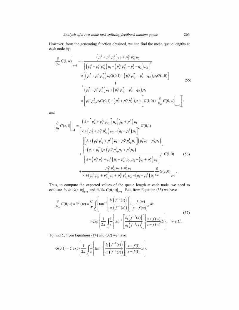
However, from the generating function obtained, we can find the mean queue lengths at each node by:

1 21 2

1 21 2

1 21 2

1 21 2

2 12 1

2 2 21 1 21 2

22 2 2 111 1 2 2 21 2

2 2 2 11 1 2 2 21 2

2 2 2 11 1 2 2 21 2

2 2 22 1 12 1

(1, )

(0,1) (1,0)

1

(0,1) (1,0)

s ss s

s sws s

s ss s

s ss s

s ss s

p p p p pG w

w p p p p p p q

p p p G p p p q G

p p p p p p q

p p G p p p G1

(0, )w

G ww

(55)

and

22

22

1 21 2

22

1 21 2

2 1 22 2 1 1 12

22 1 212 2 1 1 12

1 2 1 2 11 1 2 1 1 2 21 2

2 1 21 1 1 2 1 12

21 2 1 2

1 1 2 1 1 11 2

( ,1) (0,1)

(1,

ss

szs

s ss s

ss

s ss s

p p p q pG z G

z p p p q p

p p p p p p p

q p p p pG

p p p p p q p

22

1 21 2

1 22 1 12

1 2 1 211 1 2 1 1 11 2

0)

( ,0) .s

ss s

zs s

p p pG z

zp p p p p q p

(56)

Thus, to compute the expected values of the queue length at each node, we need to evaluate 1/ ( , 0) zz G z and 1/ (0, ) .ww G w But, from Equation (55) we have

1 '1' 121

1

111

11

( ) ( )(0, ) ( ) tan( ) ( )

( )1 1 ( )exp tan , .2 ( )( )

o

o

L

L

b f sC f wG w w ds

w a f s s f w

b f s s f wds w L

s s f wa f s

(57)

To find C, from Equations (14) and (32) we have

111

11

( )1 1 (1)(0,1) exp tan d .2 (1)( )

oL

b f s s fG C ss s fa f s


Thus,

111

11

( )1 1 (1)(0,1)exp tan d .2 (1)( )

oL

b f s s fC G ss s fa f s

(58)

To numerically evaluate Equation (57), we will parameterise G(0,w) given in Equation (32). Thus, let is e . Then, Equation (68) becomes

12 11

101

(e ) e (1)(0,1)exp tan d .2 e (1)(e )

i i

ii

b fi fC Gfa f

(59)

Thus, from Equations (55), (57) and (59) we will have:

1 '2 112101 1

( ) (1)(0, ) (0,1) tan ,( ) (1)

i

i iw

b f ei fG w G d

w a f e e f (60)

where G(0,1) is given in Equation (14). In order to numerically evaluate Equation (60), we use trapezoidal rule for the integrals on the right-hand side of Equation (62) by using K equilength subintervals of length 2 with endpoints as 2 / , 0,1, ,k k K k K

and find the derivative at w = 1. However, we need the values of 1 e kif that require

values of ( )k , 0,1, , ,k K with enough number of iterations. For instance, we may choose the number of iterations such that

510 1

max ( ) ( ) 10 .n k n kk K

(61)

Note that this condition may be revised in practice. Thus, assuming that ( )k is found (as we will show how to do so in the Algorithm below), it follows from Equation (47) and the Pelemlj-Sokhotaki formula that (see Cohen and Boxma (1983, p. 349)):

( )1 ( ( ))(e ) e , 0,1, , 1.

cos( ( ))k ki ik

kf k K (62)

The outlines of steps in the numerical evaluation of the integrals are given in the following algorithm.

5 Algorithm to compute mean queue lengths

Step 1. Choose values of and i , such that / 1, 1 , 2.i i i i

Step 2. From Equation (9), solve A(z, w) = 0 for w. This gives two roots as functions of z,say 1( )w z and 2 ( )w z .

Step 3. For z on the unit circles, choose the unique root ( )iw z , i = 1 or 2, of A(z, w) = 0 such that ( ) 1iw z .


To do this, choose z, say1/ 2 ( 3 / 2)i , such that 1z . Then, try the values of roots in Step 2 at this z, choose the one with absolute value less than or equal to 1 and call it ( )z .

Step 4. From Equation (9), solve A(z, w) = 0 for z. This gives two roots as functions of w,say 1( )z w and 2 ( )z w .

Step 5. For w on the unit circle, choose the unique root ( )iz w , i = 1 or 2, of A(z, w) = 0 such that ( ) 1iz w .

To do this, choose w, say 3 / 2 (1/ 2)i , such that 1w . Then, try the values of roots in Step 4 at this w, choose the one with absolute value less than or equal to 1 and call it ( )w . Note that ( )w is the inverse of ( )z . Thus, check to make sure that

( ( )) .w w

Step 6. From Equation (21), find ( ) Im( ( ))a w B w and ( ) ( ( )).b w Re B w

Step 7. From Step 6 and Equation (22), find a1(w) and b1(w).

Step 8. Find ( )k .

To do that, we do as follows (for more detail see Cohen and Boxma (1983, p.IV.1.3)):

Step 8.1. Set 0 ( ) 2 / , 0,1, ,k k k k k K . Using Newton’s method, solve equation

0 0 0 0( ( )) cos( ( )) ( ( )) 0 for ( ( )), 0,1, , .k k k kF k K (63)

We note that the proper choice of a starting point is very important in the Newton’s method since it is possible that the method fails. Because of this, we numerically find locations of the roots of Equation (63) through the sign of discriminant of the radical in Equation (42) and bisection method. Then, by inspection, we choose an initial value that leads to a quick convergence of the method.

Step 8.2. Using the Trapezoidal rule, find 1( )k , for each 0,1, ,k K from

21 00

1( ) ln ( ) cot d ,2k k k (64)

where 00

0

( ( ))( ( )) .

cos( ( ))The integrand in Equation (64) has a singularity at .k To deal with this

singularity, we can rewrite the integrand as:

0 0 01 1ln ( ) ln ( ) cot ln ( ) cot .2 2k k k k

The integral of the last term equals zero; the value of the first integrand at k can easily be determined by the l’Hôspital’s Rule. Therefore, the resulting integral can be


evaluated using a standard numerical integration procedure, i.e. the trapezoidal rule. Thus, we can rewrite Equation (64) as

21 0 0

0( ) ln ( ) ln ( ) cot d .

2k

k k k

In applying the trapezoidal rule, denote the integrand of the integral in Equation (64) by ( )h , i.e.

0 0( ) ln ( ) ln ( ) cot .2

kkh

Then,

20 1 1

0( )d ( ) 2 ( ) 2 ( ) 2 ( ) ( ) ,k K Kh h h h h h

K

where 2 / , 0,1, , .k k K k KTo find ( )kh , we can rewrite ( )h as

0

0

( )ln

( )( ) .

tan2

k

kh

However,

0

00

0

( )ln

( ) 2 dlim ( ) .( ) dtan

2k

k

k

k k

Therefore, for this case, we have

00

2 d( ) ( ) .( ) d

k

kk

h

Step 8.3. For 1,2, ,n repeat Step 8.1 and Step 8.2 to find ( )n k and 1( )n k ,0,1, ,k K until condition Equation (61) is satisfied. As we noted before, the condition

Equation (61) may be revised in practice. The last iteration in this process will be ( ), 0,1, , .k k K , 0,1, ,k K

Step 9. Find f(1).

To do this, use the Newton’s method and solve 1( ) 1f in [0, 1]. Thus, (1)f . Make sure that .


Step 10. Find '(1)f .

To do this, use the Trapezoidal rule for the integral on the right-hand side of Equation (52).

Step 11. From Equation (60), find 1( )kif e .

Step 12. Find 1( / ) (0, ) ww G w from Equation (58), using Trapezoidal rule.

Step 13. Find 1( / ) (1, ) ww G w from Equation (55).

Similarly, for G(z,0) we will have:

1 '2 11210

1

12 11

101

(e ) ( )( ,0) tan d(e ) e ( )

(e ) e ( )exp tan d , .2 e ( )(e )

i

i i

i i

ii

d gCi g zG z

z c g f z

d gi g zz L

g zc g

(65)

Following the same procedure as for G(0,w), we can find 1( / ) ( ,0) zz G z and then use

Equation (56) to find 1( / ) ( ,1) zz G z .

We note that in the computational process, we used N1 and N2 for service stations (nodes) 1 and 2, respectively. Thus, we refer to the activities related to computing

1( / ) ( ,1) zz G z by N1 and to 1( / ) (1, ) ww G w by N2.

6 Special case

We now consider a special case in which there is no feedback and no splitting, i.e. 1 21 1 2

1 2 21 2 0s sp p p p p . This will change our model to a standard M/M/1 in tandem with independent service times at each station and no blocking. Thus, we let / , 1,2j j j , be the traffic intensity at each station. It is well-known that the system is stable if 1, 1,2j j . For this special case, we can find the probability

( ), 1,2jQ t j , of each station to be idle at time t, t > 0, assuming that (0) 1.jQ As indicated in Cohen (1982) and Blanc (1985), ( )jQ t can be found by

0

(1/ ) ( )e ( )d , 1,2,

1 ( )j jrt

jj

rQ t t j

r (66)

where,

2

1 1 4

( ) , 1,2,2

j jj j j

jj

r r r

r j (67)


and the larger branch point of ( )j r is2

1 , 1,2.j j jr j Using the saddle

point method (see Wishart (1966)), from Equation (56) for large value of t, the asymptotic expansion of the queue length at each station is:

214

2 3

e 11 1 , 1,2 ( )1( )

1 11 , 1.

j tj j

j jjjj

jj

OttQ t

Ott

(68)

Blanc (1985, p.12) proves that for large value of t, asymptotic expansion of probability that the system is empty, i.e. 0,0 1 2( ) ( ) ( ) 0p t p t t is as follows:

1

2

1

2/4 1 21

1 2 2 31 2 11

2 1

2/4 2 12

1 20,0 2 32 1 21

1 2

/2 4

1 1 11

1 2

1 e1 12 ( )1

11 , 1,

1 e1 1( )2 ( )1

11 , 1,

1 e 11 1 1 ,2

1,

t

t

t

t

ot

P tt

ot

ott

1 2 1.

(69)

7 Numerical example

We have chosen the following fixed data: 1 0.5q , 2 0.7q , 11 0.1p ,

11 0.05Sp , 12 1

1 1 1 11 ( )Sp q p p , 11 0.5Sq ,

1 1 1

1 21 ( )S S Sp q p , 22 0.1Sp ,

21 22 2 2 21 ( )Sp q p p , 2

2 0.1p , 22 0.2p ,

2

1 0.1Sp ,2 2 2

2 11 ( )S S Sq p p . However,

we have chosen the value of parameters , 1 and 2 fixed for Tables 1 and 2 and to vary for the sake of illustration as in Table 3.


Table 111 1 2; 10, 50, 60

NRe

10

10 =

3.52

75

3.51

84

3.51

06

3.44

45

3.28

66

2.93

76

2.24

52

0.96

286

–1.2

301

–4.5

812

–9.0

555

–14.

25

–19.

482

–23.

964

–26.

984

–28.

049

4 0

3.52

35

3.51

12

3.46

03

3.44

45

3.28

66

2.93

76

2.24

52

0.96

286

–1.2

301

–4.5

812

–9.0

555

–14.

25

–19.

482

–23.

964

–26.

984

–28.

049

3 0

3.53

86

3.52

87

3.56

05

3.44

45

3.28

66

2.93

76

2.24

52

0.96

286

–1.2

301

–4.5

812

–9.0

555

–14.

25

–19.

482

–23.

964

–26.

984

–28.

049

2 0

3.52

94

3.51

25

3.36

3.44

48

3.28

66

2.93

76

2.24

52

0.96

286

–1.2

301

–4.5

812

–9.0

555

–14.

25

–19.

482

–23.

964

–26.

984

–28.

049

1 0

3.57

56

3.56

72

4.11

99

3.43

29

3.28

66

2.93

76

2.24

52

0.96

286

–1.2

301

–4.5

812

–9.0

555

–14.

25

–19.

482

–23.

964

–26.

984

–28.

049

0 0

3.54

26

3.51

`

1.65

78

3.46

54

3.28

54

2.93

76

2.24

52

0.96

286

–1.2

301

–4.5

812

–9.0

555

–14.

25

–19.

482

–23.

964

–26.

984

–28.

049

4 0

3.82

88

3.86

59

5.48

38

3.28

64

3.20

1

2.93

75

2.24

52

0.96

286

–1.2

301

–4.5

812

–9.0

555

–14.

25

–19.

482

–23.

965

–26.

985

–28.

05

3 0

5.18

46

5.22

63

5.73

11

4.05

51

3.39

21

2.95

08

2.24

52

0.96

286

–1.2

301

–4.5

876

–9.1

072

–14.

39

–19.

725

–24.

299

–27.

379

–28.

465

2 0

–1.3

109

–1.6

536

–4.3

078

1.18

32

2.44

03

2.54

67

2.24

99

0.96

567

–1.2

679

–5.4

547

–11.

696

–19.

056

–26.

404

–32.

623

–36.

774

–38.

231

1 0

11.2

17

10.8

51

9.79

32

8.15

98

6.13

58

3.96

11

1.92

24

0.37

628

–4.6

495

–23.

552

–48.

69

–75.

698

–100

.98

–121

.46

–134

.77

–139

.38

0 0

2907

.9

2844

.5

2656

.9

2353

.4

1947

.1

1455

.4

899.

87

304.

52

–304

.65

–901

.02

–145

8.5

–195

2.5

–236

1.3

–266

7

–285

6

–291

9.9

k 0 1 2 3 4 5 6 7 8 9 10 11 12 13 14 15


Table 111 1 2; 10, 50, 60

NRe (continued)

10

10 =

–26.

984

–23.

964

–19.

482

–14.

25

–9.0

555

–4.5

812

–1.2

301

0.96

286

2.24

52

2.93

76

3.28

66

3.44

45

3.51

06

3.51

84

3.52

75

4 0

–26.

984

–23.

964

–19.

482

–14.

25

–9.0

555

–4.5

812

–1.2

301

0.96

286

2.24

52

2.93

76

3.28

66

3.44

45

3.46

03

3.51

12

3.52

35

3 0

–26.

984

–23.

964

–19.

482

–14.

25

–9.0

555

–4.5

812

–1.2

301

0.96

286

2.24

52

2.93

76

3.28

66

3.44

45

3.56

05

3.52

87

3.53

86

2 0

–26.

984

–23.

964

–19.

482

–14.

25

–9.0

555

–4.5

812

–1.2

301

0.96

286

2.24

52

2.93

76

3.28

66

3.44

48

3.35

99

3.51

25

3.52

94

1 0

–26.

984

–23.

964

–19.

482

–14.

25

–9.0

555

–4.5

812

–1.2

301

0.96

286

2.24

52

2.93

76

3.28

66

3.43

29

4.12

3.56

72

3.57

56

0 0

–26.

984

–23.

964

–19.

482

–14.

25

–9.0

555

–4.5

812

–1.2

301

0.96

286

2.24

52

2.93

76

3.28

54

3.46

54

1.65

76

3.51

3.54

26

4 0

–26.

985

–23.

965

–19.

482

–14.

25

–9.0

555

–4.5

812

–1.2

301

0.96

286

2.24

52

2.93

75

3.20

1

3.28

64

5.48

35

3.86

59

3.82

88

3 0

–27.

379

–24.

299

–19.

725

–14.

39

–9.1

072

–4.5

876

–1.2

301

0.96

286

2.24

52

2.95

08

3.39

2

4.05

51

5.73

12

5.22

63

5.18

46

2 0

–36.

774

–32.

623

–26.

404

–19.

056

–11.

696

–5.4

547

–1.2

679

0.96

567

2.24

99

2.54

67

2.44

04

1.18

32

–4.3

081

–1.6

537

–1.3

11

1 0

–134

.77

–121

.46

–100

.98

–75.

698

–48.

69

–23.

552

–4.6

495

0.37

628

1.92

24

3.96

11

6.13

58

8.15

98

9.79

31

10.8

51

11.2

17

0 0

–285

6

–266

7

–236

1.3

–195

2.5

–145

8.4

–901

.01

–304

.65

304.

52

899.

86

1455

.4

1947

.1

2353

.4

2656

.9

2844

.4

2907

.8

k 16 17 18 19 20 21 22 23 24 25 26 27 28 29 30


Table 221 1 2; 10, 50, 60

NRe

10

10 =

3.93

66

3.88

46

3.71

9

3.41

68

2.95

39

2.31

53

1.50

2

0.53

247

–0.5

563

–1.7

113

–2.8

668

–3.9

499

–4.8

871

–5.6

116

–6.0

694

–6.2

261

4 0

3.93

66

3.88

46

3.71

9

3.41

68

2.95

39

2.31

53

1.50

2

0.53

247

–0.5

563

–1.7

113

–2.8

668

–3.9

499

–4.8

871

–5.6

116

–6.0

694

–6.2

261

3 0

3.93

66

3.88

46

3.71

9

3.41

68

2.95

39

2.31

53

1.50

2

0.53

247

–0.5

563

–1.7

113

–2.8

668

–3.9

499

–4.8

871

–5.6

116

–6.0

694

–6.2

261

2 0

3.93

66

3.88

46

3.71

9

3.41

68

2.95

39

2.31

53

1.50

2

0.53

247

–0.5

563

–1.7

113

–2.8

668

–3.9

499

–4.8

871

–5.6

116

–6.0

694

–6.2

261

1 0

3.93

66

3.88

46

3.71

9

3.41

68

2.95

39

2.31

53

1.50

2

0.53

247

–0.5

563

–1.7

113

–2.8

668

–3.9

499

–4.8

871

–5.6

116

–6.0

694

–6.2

261

0 0

3.93

66

3.88

46

3.71

9

3.41

68

2.95

39

2.31

53

1.50

2

0.53

247

–0.5

563

–1.7

113

–2.8

668

–3.9

499

–4.8

871

–5.6

116

–6.0

694

–6.2

261

4 0

3.93

66

3.88

46

3.71

9

3.41

68

2.95

39

2.31

53

1.50

2

0.53

247

–0.5

563

–1.7

113

–2.8

668

–3.9

499

–4.8

871

–5.6

116

–6.0

694

–6.2

261

3 0

3.93

66

3.88

46

3.71

9

3.41

68

2.95

39

2.31

53

1.50

2

0.53

247

–0.5

563

–1.7

113

–2.8

668

–3.9

499

–4.8

871

–5.6

116

–6.0

694

–6.2

261

2 0

3.93

66

3.88

46

3.71

9

3.41

68

2.95

39

2.31

53

1.50

2

0.53

247

–0.5

563

–1.7

113

–2.8

668

–3.9

499

–4.8

871

–5.6

116

–6.0

695

–6.2

261

1 0

3.93

8

3.88

48

3.71

91

3.41

7

2.95

41

2.31

55

1.50

21

0.53

247

–0.5

564

–1.7

116

–2.8

683

–3.9

543

–4.8

958

–5.6

244

–6.0

845

–6.2

403

0 0

4.00

76

3.91

66

3.74

89

3.46

16

3.02

58

2.41

6

1.60

95

0.59

046

–0.6

424

–2.0

645

–3.6

129

–5.1

759

–6.5

971

–7.6

998

–8.3

321

–8.4

141

k 0 1 2 3 4 5 6 7 8 9 10 11 12 13 14 15


Table 221 1 2; 10, 50, 60

NRe (continued)

10

10 =

–6.0

694

–5.6

116

–4.8

871

–3.9

499

–2.8

668

–1.7

113

–0.5

563

0.53

247

1.50

2

2.31

53

2.95

39

3.41

68

3.71

9

3.88

46

3.93

66

4 0

–6.0

694

–5.6

116

–4.8

871

–3.9

499

–2.8

668

–1.7

113

–0.5

563

0.53

247

1.50

2

2.31

53

2.95

39

3.41

68

3.71

9

3.88

46

3.93

66

3 0

–6.0

694

–5.6

116

–4.8

871

–3.9

499

–2.8

668

–1.7

113

–0.5

563

0.53

247

1.50

2

2.31

53

2.95

39

3.41

68

3.71

9

3.88

46

3.93

66

2 0

–6.0

694

–5.6

116

–4.8

871

–3.9

499

–2.8

668

–1.7

113

–0.5

563

0.53

247

1.50

2

2.31

53

2.95

39

3.41

68

3.71

9

3.88

46

3.93

66

1 0

–6.0

694

–5.6

116

–4.8

871

–3.9

499

–2.8

668

–1.7

113

–0.5

563

0.53

247

1.50

2

2.31

53

2.95

39

3.41

68

3.71

9

3.88

46

3.93

66

0 0

–6.0

694

–5.6

116

–4.8

871

–3.9

499

–2.8

668

–1.7

113

–0.5

563

0.53

247

1.50

2

2.31

53

2.95

39

3.41

68

3.71

9

3.88

46

3.93

66

4 0

–6.0

694

–5.6

116

–4.8

871

–3.9

499

–2.8

668

–1.7

113

–0.5

563

0.53

247

1.50

2

2.31

53

2.95

39

3.41

68

3.71

9

3.88

46

3.93

66

3 0

–6.0

694

–5.6

116

–4.8

871

–3.9

499

–2.8

668

–1.7

113

–0.5

563

0.53

247

1.50

2

2.31

53

2.95

39

3.41

68

3.71

9

3.88

46

3.93

66

2 0

–6.0

695

–5.6

116

–4.8

871

–3.9

499

–2.8

668

–1.7

113

–0.5

563

0.53

247

1.50

2

2.31

53

2.95

39

3.41

68

3.71

9

3.88

47

3.93

68

1 0

–6.0

803

–5.6

182

–4.8

903

–3.9

51

–2.8

67

–1.7

113

–0.5

563

0.53

247

1.50

2

2.31

53

2.95

39

3.41

74

3.72

33

3.90

07

3.96

55

0 0

–7.9

612

–7.0

702

–5.8

809

–4.5

352

–3.1

506

–1.8

117

–0.5

723

0.53

746

1.50

3

2.31

93

2.98

62

3.50

53

3.87

85

4.10

68

4.18

96

k 16 17 18 19 20 21 22 23 24 25 26 27 28 29 30


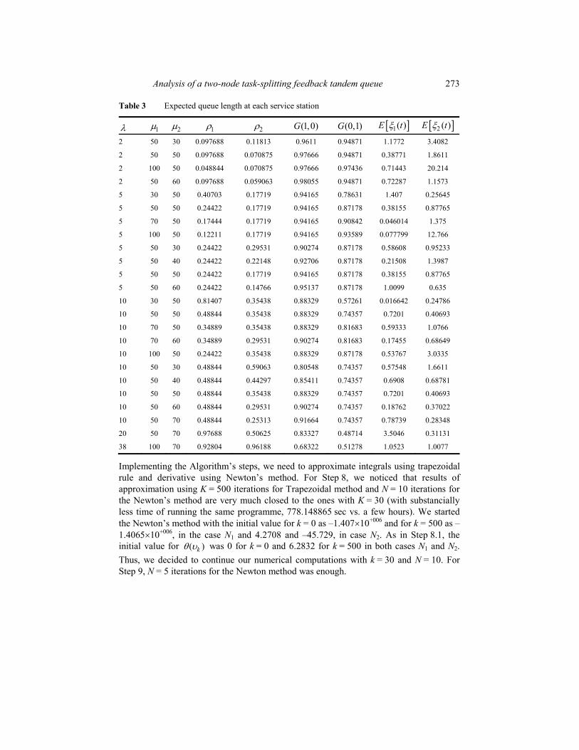
Table 3 Expected queue length at each service station

1 2 1 2 (1,0)G (0,1)G 1( )E t 2 ( )E t

2 50 30 0.097688 0.11813 0.9611 0.94871 1.1772 3.4082

2 50 50 0.097688 0.070875 0.97666 0.94871 0.38771 1.8611

2 100 50 0.048844 0.070875 0.97666 0.97436 0.71443 20.214

2 50 60 0.097688 0.059063 0.98055 0.94871 0.72287 1.1573

5 30 50 0.40703 0.17719 0.94165 0.78631 1.407 0.25645

5 50 50 0.24422 0.17719 0.94165 0.87178 0.38155 0.87765

5 70 50 0.17444 0.17719 0.94165 0.90842 0.046014 1.375

5 100 50 0.12211 0.17719 0.94165 0.93589 0.077799 12.766

5 50 30 0.24422 0.29531 0.90274 0.87178 0.58608 0.95233

5 50 40 0.24422 0.22148 0.92706 0.87178 0.21508 1.3987

5 50 50 0.24422 0.17719 0.94165 0.87178 0.38155 0.87765

5 50 60 0.24422 0.14766 0.95137 0.87178 1.0099 0.635

10 30 50 0.81407 0.35438 0.88329 0.57261 0.016642 0.24786

10 50 50 0.48844 0.35438 0.88329 0.74357 0.7201 0.40693

10 70 50 0.34889 0.35438 0.88329 0.81683 0.59333 1.0766

10 70 60 0.34889 0.29531 0.90274 0.81683 0.17455 0.68649

10 100 50 0.24422 0.35438 0.88329 0.87178 0.53767 3.0335

10 50 30 0.48844 0.59063 0.80548 0.74357 0.57548 1.6611

10 50 40 0.48844 0.44297 0.85411 0.74357 0.6908 0.68781

10 50 50 0.48844 0.35438 0.88329 0.74357 0.7201 0.40693

10 50 60 0.48844 0.29531 0.90274 0.74357 0.18762 0.37022

10 50 70 0.48844 0.25313 0.91664 0.74357 0.78739 0.28348

20 50 70 0.97688 0.50625 0.83327 0.48714 3.5046 0.31131

38 100 70 0.92804 0.96188 0.68322 0.51278 1.0523 1.0077

Implementing the Algorithm’s steps, we need to approximate integrals using trapezoidal rule and derivative using Newton’s method. For Step 8, we noticed that results of approximation using K = 500 iterations for Trapezoidal method and N = 10 iterations for the Newton’s method are very much closed to the ones with K = 30 (with substancially less time of running the same programme, 778.148865 sec vs. a few hours). We started the Newton’s method with the initial value for k = 0 as –1.407 10+006 and for k = 500 as –1.4065 10+006, in the case N1 and 4.2708 and –45.729, in case N2. As in Step 8.1, the initial value for ( )k was 0 for k = 0 and 6.2832 for k = 500 in both cases N1 and N2.Thus, we decided to continue our numerical computations with k = 30 and N = 10. For Step 9, N = 5 iterations for the Newton method was enough.


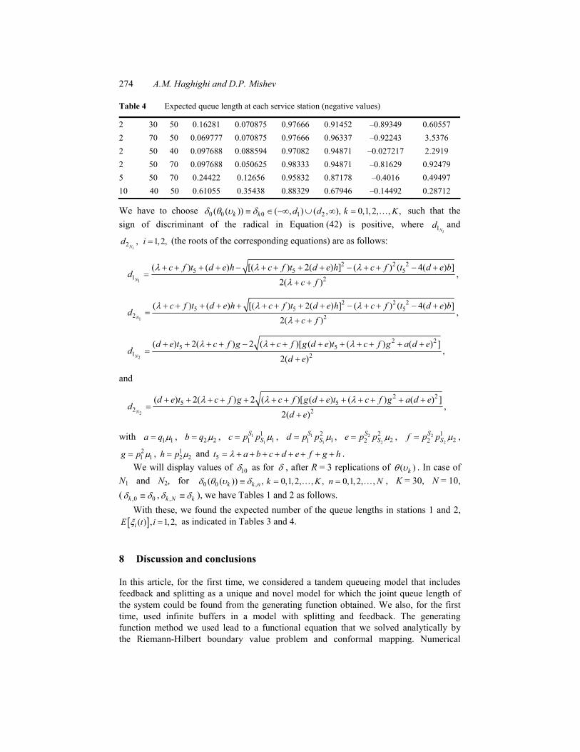
Table 4 Expected queue length at each service station (negative values)

2 30 50 0.16281 0.070875 0.97666 0.91452 –0.89349 0.60557 2 70 50 0.069777 0.070875 0.97666 0.96337 –0.92243 3.5376 2 50 40 0.097688 0.088594 0.97082 0.94871 –0.027217 2.2919 2 50 70 0.097688 0.050625 0.98333 0.94871 –0.81629 0.92479 5 50 70 0.24422 0.12656 0.95832 0.87178 –0.4016 0.49497 10 40 50 0.61055 0.35438 0.88329 0.67946 –0.14492 0.28712

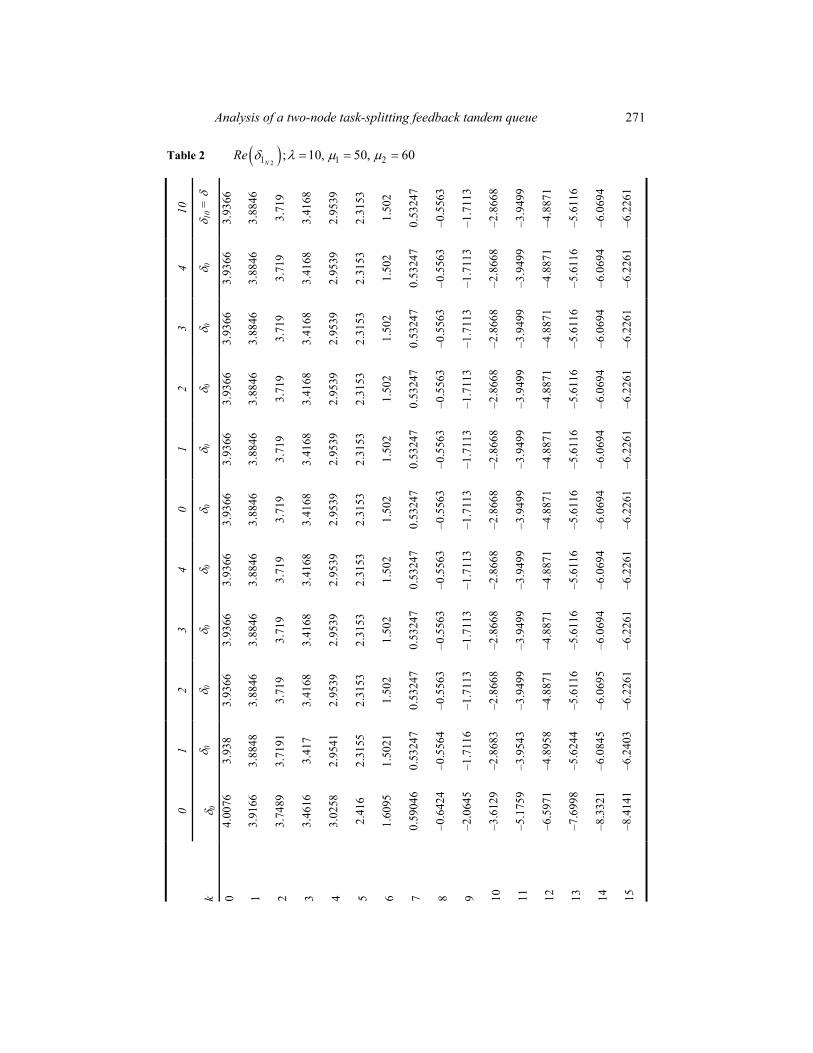
We have to choose 0 0 0 1 2( ( )) ( , ) ( , ), 0,1,2, , ,k k d d k K such that the sign of discriminant of the radical in Equation (42) is positive, where 1Ni

d and

2 ,Ni

d 1,2,i (the roots of the corresponding equations) are as follows:

1

2 2 25 5 5

1 2

( ) ( ) [( ) 2( ) ] ( ) ( 4( ) ],

2( )N

c f t d e h c f t d e h c f t d e bd

c f

1

2 2 25 5 5

2 2

( ) ( ) [( ) 2( ) ] ( ) ( 4( ) ],

2( )N

c f t d e h c f t d e h c f t d e bd

c f

2

2 25 5

1 2

( ) 2( ) 2 ( )[ ( ) ( ) ( ) ],

2( )N

d e t c f g c f g d e t c f g a d ed

d e

and

2

2 25 5

2 2

( ) 2( ) 2 ( )[ ( ) ( ) ( ) ],

2( )N

d e t c f g c f g d e t c f g a d ed

d e

with 1 1a q , 2 2b q , 11

111

SSc p p , 1

1

211

SSd p p , 2

2

222

SSe p p , 2

2

122

SSf p p ,

21 1g p , 1

2 2h p and 5t a b c d e f g h .We will display values of 10 as for , after R = 3 replications of ( )k . In case of

N1 and N2, for 0 0 ,( ( )) , 0,1, 2, , , 0,1, 2, ,k k n k K n N , K = 30, N = 10, ( ,0 0k , ,k N k ), we have Tables 1 and 2 as follows.

With these, we found the expected number of the queue lengths in stations 1 and 2, ( ) , 1,2,iE t i as indicated in Tables 3 and 4.

8 Discussion and conclusions

In this article, for the first time, we considered a tandem queueing model that includes feedback and splitting as a unique and novel model for which the joint queue length of the system could be found from the generating function obtained. We also, for the first time, used infinite buffers in a model with splitting and feedback. The generating function method we used lead to a functional equation that we solved analytically by the Riemann-Hilbert boundary value problem and conformal mapping. Numerical


computation for our model was a challenging task. Yet, we were able to find the mean queue length at each node algorithmically by the generating function obtained. Thus, while we have offered, for the first time, an algorithm for numerical computation of the mean queue lengths, an exact distribution of the queue length, that is computationally practical, remains to be an open problem.

As it was mentioned earlier, the splitting feature was considered in a parallel queueing system. Here, in this article, we included this feature in the tandem queue. Thus, including such a novel feature in a combined parallel and tandem queueing system, remains to be considered.

Considering the data we have chosen, these results show that the model is quite efficient as such with all feedbacks and splitting, the queue length at each station is moderately low. In case 10 , 1 50 , 2 60 , for instance, the expected number of the queue lengths in stations 1 and 2 as 0.18762 and 0.37022, respectively, with substancially less time of running the same programme, 778.148865 sec, vs. a few hours. The probability that the first station is busy while the second is empty is 0.90274. On the other hand, the probability that the second station is busy while the first is empty is 0.74357. Even with very high traffic intensity such as in case 38 , 1 100 , 2 70 , 1 0.92804 , 2 0.96188 , the probability that the first station is busy while the second is empty is 0.68322, while the probability that the second station is busy while the first is empty is 0.51278. The expected queue lengths in stations 1 and 2, in this case are 1.0523 and 1.0077, respectively.

We did, however, observed that there are parameter-values for which results were not acceptable. For instance, see Table 4 for some such values. Theses values seems when we have very low traffic intensity or relatively high one, although, in some cases of the later, no problem was observed. We have noticed that negativity is on the expected value in station 1.

As a final observation, note that when the speed of service increases in the first station, the second service station becomes highly conjested, which intutively makes sences.

Acknowledgement

The authors wish to thank the reviewer for comments that improved the quality of the article.

References Artalejo, J.R. (1999) ‘A classified bibliography of research on retrial queues’, Progress in

1990–1999, Vol. 7, pp.187–211. Blanc, J.P.C. (1985) ‘The relaxation time of two queueing systems in series’, Communications in

Statististics – Stochastic Models, Vol. 1, pp.1–16. Brockett, R.W., Weibo, G. and Yang G. (1999) ‘Stochastic analysis for fluid queueing systems’,

Paper presented in the Proceedings of the 38th Conference on Decision and Control, Phoenix, Arizona USA, December, pp.3077–3082, IEEE 0-7803-5250-5/9.

Burke, P.J. (1956) ‘The output of a queueing system’, Operations Research, Vol. 4, pp.699–704.


Ceder, A. and Kobi E. (2002) ‘Optimal distance between two branches of uncontrolled split intersection’, Transportation Research Park A, Vol. 36, pp.699–724.

Cohen, J.W. (1982) The Single Server Queue (2nd ed). Amesterdam, NL: North-Holand Publ. Co. Cohen, J.W. (1988) ‘Boundary value problems in queueing theory’, Queueing Systems, Vol. 3,

pp.97–128. Cohen, J.W. and Boxma, O.J. (1983) Boundary Value Problems in Queueing System Analysis.

Amesterdam, NL: North-Holand. Diamond, J. and Alfa, A.S. (1998) ‘The MAP/PH/1 retrial queue’, Communications in Statististics

– Stochastic Models, Vol. 14, pp.1151–1178. Fayolle, G. (1979) ‘Méthodes analytiques pour les filess d'attente couplées’, Theses, Université

Paris VI. Fayolle, G. and Iasnogorodski, R. (1979) ‘Two coupled processors: the reduction to a Riemann-

Hilbert problem’, Z. Wahrscheinlichkeitsth, Vol. 47, pp.325–351. Fayolle, G., King, P.J.B. and Mitrani, I. (1982) ‘The solution of certain two-dimensional Markov

models’, Advances in Applied Probability, Vol. 14, pp.295–308. Gakhov, F.D. (1966) Boundary Value Problems. Oxford, UK: Pergamon Press. Grassmann, W.K. and Drekic, S. (2000) ‘An analytic solution for a tamdem queue with blocking’,

Queueing Systems, Vol. 36, pp.221–235. Haghighi, A.M. and Mishev, D.P. (2007) ‘A tandem queueing system with task-splitting, feedback

and blocking’, Int. J. Operational Research, Vol. 2, pp.208–230. Iasnogorodski, R. (1979) ‘Problèmes-frontiers dans les files d'attente’, Theses, Université Paris VI. Jackson, J.R. (1957) ‘Networks of waiting lines’, Operations Research, Vol. 5, pp.518–521. Jeffe, S. (1992) ‘The equilibrium distribution for a clocked buffered switch’, Probability in the

Engineering and Informational Sciences, Vol. 6, pp.425–438. Kist, A.A., Lloyd-Smith, B. and Harris, R.J. (2005) ‘A simple IP flow blocking model’, The 19th

International Teletraffic Congress (ITC 19), Beijing, China. Klimenok, V.I. and Taramin, O.S. (2007) ‘A tandem queueing system with loss and blocking’,

Applied and Computational Mathematics, Vol. 6, pp.295–311. Konhein, A.G. and Reiser, M. (1976) ‘A queueing model with finite waiting room and blocking’,

Journal of the Association for Computing Machinery, Vol. 23, pp.328–341. Konhein, A.G. and Reiser, M. (1978) ‘Finite capacity queueing systems with applications in

computer modeling’, Society for Industrial and Applied Mathematics Journal of Computing,Vol. 7, pp.210–220.

Krantz, S.G. (1992) Function Theory of Several Complex Variables. Providence, RI: AMS Chelsea Publishing.

Latouche, G., and Neuts, M.F. (1980) ‘Efficient algorithmic solution of exponential tandem queues with blocking’, Society for Industrial and Applied Mathematics Journal Algebra Discrete Methods, Vol. 1, pp.93–106.

Mikou, N. (1988) ‘Two-node jackson’s network’, Communications in Statististics – Stochastic Models, Vol. 4, pp.523–552.

Miyazawa, M., Sakume, Y. and Yamaguchi, S. (2007) ‘Asymptotic behaviors of the loss probability for a finite buffer queue with QBD structure’, Stochastic Models, Vol. 23, pp.79–95.

Montazer-Haghighi, A. (1976) ‘Many-server queueing systems with feedback’, PhD Dissertation,Case Western Reserve University, microfilm published by UMI Dissertation Services, from Proquest, Ann Arbor, Michigan, www.il.proquest.com.

Muskhelishvili, N.I. (1953) J.R.M. Radok (Ed), Singular Integral Equations: Boundary Problems of Function Theory and Their Application to Mathematics Physics (2nd ed., 1946), translated from Russian in English, Groningen, Holland: P. Noordhoff N.V.


Resing, J.A.C. and Örmeci, L. (2003) ‘A tandem queueing model with coupled processors’, Operations Research Letters, Vol. 31, pp.383–389.

Smirnov, V.I. (1964) A Course of Higher Mathematics. Oxford, UK: Pergamon Press, Vol. 3 Part 2.

Takács, L. (1962) Introduction to the Theory of Queue. New York, NY: Oxford University Press. Tang, J. and Zhao, Y.Q. (2008) ‘Stationary tail asymptotics of a tandem queue with feedback’.

Annals of Operation Research, Vol. 160, pp.173–189. Van Leeuwaarden, J.S.H. and Resing, J.A. (2005) ‘A tandem queue with couple processors:

computational issues’, Queueing Systems, Vol. 50, pp.29–52. Wishart, D.M.G. (1966) ‘Discussion on Kingman’s paper’, Journal of Royal Statistical Society

Series B, Vol. 28, pp.442–443.

Analysis of a two-node task-splitting feedback tandem queue with infinite buffers by functional...

Documents

Transcript of Analysis of a two-node task-splitting feedback tandem queue with infinite buffers by functional...