Single-Forward-Step Projective Splitting: ExploitingCocoercivity

Patrick R. Johnstone∗ Jonathan Eckstein∗

August 24, 2020

Abstract

This work describes a new variant of projective splitting for solving maximal mono-tone inclusions and complicated convex optimization problems. In the new version,cocoercive operators can be processed with a single forward step per iteration. Inthe convex optimization context, cocoercivity is equivalent to Lipschitz differentiabil-ity. Prior forward-step versions of projective splitting did not fully exploit cocoercivityand required two forward steps per iteration for such operators. Our new single-forward-step method establishes a symmetry between projective splitting algorithms,the classical forward-backward splitting method (FB), and Tseng’s forward-backward-forward method (FBF). The new procedure allows for larger stepsizes for cocoerciveoperators: the stepsize bound is 2β for a β-cocoercive operator, the same bound as hasbeen established for FB. We show that FB corresponds to an unattainable boundarycase of the parameters in the new procedure. Unlike FB, the new method allows for abacktracking procedure when the cocoercivity constant is unknown. Proving conver-gence of the algorithm requires some departures from the prior proof framework forprojective splitting. We close with some computational tests establishing competitiveperformance for the method.

1 Introduction

1.1 Problem Statement

For a collection of real Hilbert spaces {Hi}ni=0 consider the finite-sum convex minimizationproblem:

minx∈H0

n∑i=1

(fi(Gix) + hi(Gix)

), (1)

where every fi : Hi → (−∞,+∞] and hi : Hi → R is closed, proper, and convex, every hi isalso differentiable with Li-Lipschitz-continuous gradients, and the operators Gi : H0 → Hi

∗Department of Management Science and Information Systems, Rutgers Business School Newark and NewBrunswick, Rutgers University. Contact: patrick.r.johnstone@gmail.com, jeckstei@business.rutgers.edu

1

arX

iv:1

902.

0902

5v3

[m

ath.

OC

] 2

0 A

ug 2

020

are linear and bounded. Under appropriate constraint qualifications, (1) is equivalent to themonotone inclusion problem of finding z ∈ H0 such that

0 ∈n∑i=1

G∗i (Ai +Bi)Giz (2)

where all Ai : Hi → 2Hi and Bi : Hi → Hi are maximal monotone and each Bi is L−1i -cocoercive, meaning that it is single-valued and

Li〈Bix1 −Bix2, x1 − x2〉 ≥ ‖Bix1 −Bix2‖2

for some Li ≥ 0. (When Li = 0, Bi must be a constant operator, that is, there is some vi ∈ Hi

such that Bix = vi for all x ∈ Hi. ) In particular, if we set Ai = ∂fi (the subgradient mapof fi) and Bi = ∇hi (the gradient of hi) then the solution sets of the two problems coincideunder a special case of the constraint qualification of [9, Prop. 5.3].

Defining Ti = Ai +Bi for all i, problem (2) may be written as

0 ∈n∑i=1

G∗iTiGiz. (3)

This more compact problem statement will be used occasionally in our analysis below.

1.2 Background

Operator splitting algorithms are an effective way to solve structured convex optimizationproblems and monotone inclusions such as (1), (2), and (3). Their defining feature is thatthey decompose a problem into a set of manageable pieces. Each iteration consists of rel-atively easy calculations confined to each individual component of the decomposition, inconjunction with some simple coordination operations orchestrated to converge to a so-lution. Arguably the three most popular classes of operator splitting algorithms are theforward-backward splitting (FB) [11], Douglas/Peaceman-Rachford splitting (DR) [26], andforward-backward-forward (FBF) [40] methods. Indeed, many algorithms in convex opti-mization and monotone inclusions are in fact instances of one of these methods. The popularAlternating Direction Method of Multipliers (ADMM), in its standard form, can be viewedas a dual implementation of DR [20].

Projective splitting is a relatively recent and currently less well-known class of operatorsplitting methods, operating in a primal-dual space. Each iteration k of these methodsexplicitly contructs an affine “separator” function ϕk for which ϕk(p) ≤ 0 for every p inthe set S of primal-dual solutions. The next iterate pk+1 is then obtained by projecting thecurrent iterate pk onto the halfspace defined by ϕk(p) ≤ 0, possibly with some over- or under-relaxation. Crucially, ϕk is obtained by performing calculations that consider each operatorTi separately, so that the procedures are indeed operator splitting algorithms. In the originalformulations of projective splitting [18, 19], the calculation applied to each operator Ti wasa standard resolvent operation, also known as a “backward step”. Resolvent operationsremained the only way to process individual operators as projective splitting was generalizedto cover compositions of maximal monotone operators with bounded linear maps [1] — as in

2

the Gi in (3) — and block-iterative (incremental) or asynchronous calculation patterns [10,17]. Convergence rate and other theoretical results regarding projective splitting may befound in [22, 23, 28, 29].

The algorithms in [39, 21] were the first to construct projective splitting separators byapplying calculations other than resolvent steps to the operators Ti. In particular, [21]developed a procedure that could instead use two forward (explicit or gradient) steps for op-erators Ti that are Lipschitz continuous. However, that result raised a question: if projectivesplitting can exploit Lipschitz continuity, can it further exploit the presence of cocoerciveoperators? Cocoercivity is in general a stronger property than Lipschitz continuity. How-ever, when an operator is the gradient of a closed proper convex function (such as hi in (1)),the Baillon-Haddad theorem [2, 3] establishes that the two properties are equivalent: ∇hi isLi-Lipschitz continuous if and only if it is L−1i -cocoercive.

Operator splitting methods that exploit cocoercivity rather than mere Lipschitz continu-ity typically have lower per-iteration computational complexity and a larger range of permis-sible stepsizes. For example, both FBF and the extragradient (EG) method [25] only requireLipchitz continuity, but need two forward steps per iteration and limit the stepsize to L−1,where L is the Lipschitz constant. If one strengthens the assumption to L−1-cocoercivity,one can instead use FB, which only needs one forward step per iteration and allows stepsizesbounded away from 2L−1. One departure from this pattern is the recently developed methodof [31], which only requires Lipschitz continuity but uses just one forward step per iteration.While this property is remarkable, it should be noted that its stepsizes must be boundedby (1/2)L−1, which is half the allowable stepsize for EG or FBF and just a fourth of FB’sstepsize range.

Much like EG and FBF, the projective splitting computation in [21] requires Lipschitzcontinuity1, two forward steps per iteration, and limits the stepsize to be less than L−1 (whennot using backtracking). Considering the relationship between FB and FBF/EG leads tothe following question: is there a variant of projective splitting which converges under thestronger assumption of L−1-cocoercivity, while processing each cocoercive operator with asingle forward step per iteration and allowing stepsizes bounded above by 2L−1?

This paper shows that the answer to this question is “yes”. Referring to (2), the newprocedure analyzed here requires one forward step on Bi and one resolvent for Ai at eachiteration. In the context of (1), the new procedure requires one forward step on ∇hi and oneproximal operator evaluation on fi. When the resolvent is easily computable (for example,when Ai is the zero map and its resolvent is simply the identity), the new procedure caneffectively halve the computation necessary to run the same number of iterations as theprevious procedure of [21]. This advantage is equivalent to that of FB over FBF and EGwhen cocoercivity is present. Another advantage of the proposed method is that it allowsfor a backtracking linesearch when the cocoercivity constant is unknown, whereas no suchvariant of general cocoercive FB is currently known.

The analysis of this new method is significantly different from our previous work in[21], using a novel “ascent lemma” (Lemma 17) regarding the separators generated by thealgorithm. The new procedure also has an interesting connection to the original resolvent

1If backtracking is used, then all three of these methods can converge under weaker local continuityassumptions.

3

calculation used in the projective splitting papers [18, 19, 1, 10]: in Section 2.2 below, weshow that the new procedure is equivalent to one iteration of FB applied to evaluating theresolvent of Ti = Ai+Bi. That is, we can use a single forward-backward step to approximatethe operator-processing procedure of [18, 19, 1, 10], but still obtain convergence.

The new procedure has significant potential for asynchronous and incremental implemen-tation following the ideas and techniques of previous projective splitting methods [10, 17, 21].To keep the analysis relatively manageable, however, we plan to develop such generalizationsin a follow-up paper. Here, we will simply assume that every operator is processed once periteration.

1.3 The Optimization Context

For optimization problems of the form (1), our proposed method is a first-order proximalsplitting method that “fully splits” the problem: at each iteration, it utilizes the proximaloperator for each nonsmooth function fi, a single evaluation of the gradient ∇hi for eachsmooth function hi, and matrix-vector multiplications involving Gi and G∗i . There is no needfor any form of matrix inversion, nor to use resolvents of composed functions like fi ◦ Gi,which may in general be much more challenging to evaluate than resolvents of the fi. Thus,the method achieves the maximum possible decoupling of the elements of (1). There arealso no assumptions on the rank, row spaces, or columns spaces of the Gi. Beyond the basicresolvent, gradient, and matrix-vector multiplication operations invoked by our algorithm,the only computations at each iteration are a constant number of inner products, norms,scalar multiplications, and vector additions, all of which can all be carried out within flopcounts linear in the dimension of each Hilbert space.

Besides projective splitting approaches, there are a few first-order proximal splittingmethods that can achieve full splitting on (1). The most similar to projective splitting arethose in the family of primal-dual (PD) splitting methods; see [13, 12, 7, 35] and refer-ences therein. In fact, projective splitting is also a kind of primal-dual method, since itproduces primal and dual sequences jointly converging to a primal-dual solution. However,the convergence mechanisms are different: PD methods are usually constructed by applyingan established operator splitting technique such as FB, FBF, or DR to an appropriatelyformulated primal-dual inclusion in a primal-dual product space, possibly with a speciallychosen metric. Projective splitting methods instead work by projecting onto (or through)explicitly constructed separating hyperplanes in the primal-dual space.

There are several potential advantages of our proposed method over the more establishedPD schemes. First, unlike the PD methods, the norms ‖Gi‖ do not effect the stepsize con-straints of our proposed method, making such constraints easier to satisfy. Furthermore,projective splitting’s stepsizes may vary at each iteration and may differ for each operator.In general, projective splitting methods allow for asynchronous parallel and incrementalimplementations in an arguably simpler way than PD methods (although we do not de-velop this aspect of projective splitting in this paper). Projective splitting methods canincorporate deterministic block-iterative and asynchronous assumptions [10, 17], resultingin deterministic convergence guarantees, with the analysis being similar to the synchronouscase. In contrast, existing asynchronous and block-coordinate analyses of PD methods re-quire stochastic assumptions which only lead to probabilistic convergence guarantees [35].

4

1.4 Notation and a Simplifying Assumption

We use the same general notation as in [21, 23, 22]. Summations of the form∑n−1

i=1 ai willappear throughout this paper. To deal with the case n = 1, we use the standard conventionthat

∑0i=1 ai = 0.

We will use a boldface w = (w1, . . . , wn−1) for elements of H1 × . . . × Hn−1. Let H ,H0 × H1 × · · · × Hn−1, which we refer to as the “collective primal-dual space”, and notethat the assumption on Gn implies that Hn = H0. We use p to refer to points in H, sop , (z,w) = (z, w1, . . . , wn−1).

Throughout, we will simply write ‖ · ‖i = ‖ · ‖ as the norm for Hi and let the subscriptbe inferred from the argument. In the same way, we will write 〈·, ·〉i as 〈·, ·〉 for the innerproduct of Hi. For the collective primal-dual space we will use a special norm and innerproduct with its own subscript defined in (16).

We use the standard “⇀” notation to denote weak convergence, which is of course equiv-alent to ordinary convergence in finite-dimensional settings.

For the definition of maximal monotone operators and their basic properties, we referto [4]. For any maximal monotone operator A and scalar ρ > 0, we will use the notationJρA , (I + ρA)−1, to denote the resolvent operator, also known as the backward or implicitstep with respect to A. Thus,

x = JρA(t) ⇐⇒ x+ ρa = t and a ∈ Ax, (4)

the x and a satisfying this relation being unique. Furthermore, JρA is defined everywhere andrange(JA) = dom(A) [4, Prop. 23.2]. If A = ∂f for a closed, convex, and proper functionf , the resolvent is often referred to as the proximal operator and written as Jρ∂f = proxρf .Computing the proximal operator requires solving

proxρf (t) = arg minz

{ρf(z) +

1

2‖z − t‖2

}.

Many functions encountered in applications to machine learning and signal processing haveproximal operators which can be computed exactly with low computational complexity. Inthis paper, for a single-valued maximal monotone operator A, a forward step (also known asan explicit step) refers to the direct evaluation of Ax (or ∇f(x) in convex optimization) aspart of an algorithm.

For the rest of the paper, we will impose the simplifying assumption

Gn : Hn → Hn , I (the identity operator).

As noted in [21], the requirement that Gn = I is not a very restrictive assumption. Forexample, one can always enlarge the original problem by one operator, setting An = Bn = 0.

2 Projective Splitting

The goal of our algorithm will be to find a point in

S ,{

(z, w1, . . . , wn−1) ∈H∣∣ (∀ i ∈ {1, . . . , n− 1}) wi ∈ TiGiz, −

∑n−1i=1 G

∗iwi ∈ Tnz

}.(5)

5

It is clear that z∗ solves (2)–(3) if and only if there exist w∗1, . . . , w∗n−1 such that

(z∗, w∗1, . . . , w∗n−1) ∈ S.

Under reasonable assumptions, the set S is closed and convex; see Lemma 2. S is oftencalled the Kuhn-Tucker solution set of problem (3).

A separator-projector algorithm for finding a point in S (and hence a solution to (3))will, at each iteration k, find a closed and convex set Hk which separates S from the currentpoint, meaning S is entirely in the set (preferably, the current point is not). One can thenattempt to “move closer” to the solution set by projecting the current point onto the setHk. This general setup guarantees that the sequence generated by the method is Fejermonotone [8] with respect to S. This alone is not sufficient to guarantee that the iteratesactually converge to a point in the solution set. To establish this, one needs to show thatthe set Hk “sufficiently separates” the current point from the solution set, or at least doesso sufficiently often. Such “sufficient separation” allows one to establish that any weaklyconvergent subsequence of the iterates must have its limit in the set S, from which overallweak convergence follows from [8, Prop. 2].

With S as in (5), the separator formulation presented in [10] constructs the halfspace Hk

using the function ϕk : H→ R defined as

ϕk(z, w1, . . . , wn−1) ,n−1∑i=1

〈Giz − xki , yki − wi〉+

⟨z − xni , yni +

n−1∑i=1

G∗iwi

⟩(6)

=

⟨z,

n∑i=1

G∗i yki

⟩+

n−1∑i=1

〈xki −Gixkn, wi〉 −

n∑i=1

〈xki , yki 〉, (7)

for some auxiliary points (xki , yki ) ∈ H2

i . These points (xki , yki ) will be specified later and must

be chosen at each iteration in a specific manner guaranteeing the validity of the separatorand convergence to S. Among other properties, they must be chosen so that yki ∈ Tixki fori = 1, . . . , n. Under this condition, it follows readily that ϕk has the promised separatorproperties:

Lemma 1. The function ϕk defined in (6) is affine, and if yki ∈ Tixki for all i = 1, . . . , n,then ϕk(z, w1, . . . , wn−1) ≤ 0 for all (z, w1, . . . , wn−1) ∈ S.

Proof. That ϕk is affine is clear from its expression in (7). Now suppose that yki ∈ Tixki forall i = 1, . . . , n and p = (z, w1, . . . , wn−1) ∈ S. Then

ϕk(p) = −

(n−1∑i=1

〈Giz − xki , wi − yki 〉+ 〈z − xni , wn − yni 〉

), (8)

where wn , −∑n−1

i=1 G∗iwi. From (z, w1, . . . , wn−1) ∈ S and the definition of S, one has that

wi ∈ Tiz for all i = 1, . . . , n − 1, as well as wn ∈ Tnz. Since yi ∈ Tixi for i = 1, . . . , n,it follows from the monotonicity of T1, . . . , Tn that every inner product displayed in (8) isnonnegative, and so ϕk(p) ≤ 0.

6

S

pk = (zk, wk1 , . . . , w

kn−1)ϕk(p) = 0

ϕk(p) > 0ϕk(p) ≤ 0

Figure 1: Properties of the hyperplane {p ∈H | ϕk(p) = 0} obtained from the affine func-tion ϕk. This hyperplane is the boundary of the halfspace Hk, and it always holds thatϕk(p

∗) ≤ 0 for every p∗ ∈ S. When ϕk(pk) > 0 (as shown), the hyperplane separates the

current point pk from the solution set S.

pk = (zk, wk1 , . . . , w

kn−1)ϕk(p) = 0

pk+1

pk+2

ϕk+1(p) = 0

S

Figure 2: The basic operation of the method. Each iteration k constructs a separator ϕkas shown in Figure 1 and then obtains the next iteration by projecting onto the halfspaceHk = {p ∈H | ϕk(p) ≤ 0}, within which the solution set S is known to lie.

7

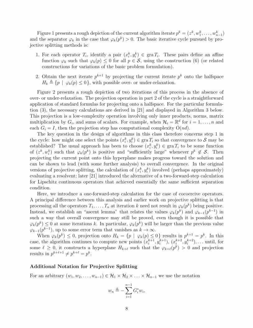
Figure 1 presents a rough depiction of the current algorithm iterate pk = (zk, wk1 , . . . , wkn−1)

and the separator ϕk in the case that ϕk(pk) > 0. The basic iterative cycle pursued by pro-

jective splitting methods is:

1. For each operator Ti, identify a pair (xki , yki ) ∈ graTi. These pairs define an affine

function ϕk such that ϕk(p) ≤ 0 for all p ∈ S, using the construction (6) (or relatedconstructions for variations of the basic problem formulation).

2. Obtain the next iterate pk+1 by projecting the current iterate pk onto the halfspaceHk , {p | ϕk(p) ≤ 0}, with possible over- or under-relaxation.

Figure 2 presents a rough depiction of two iterations of this process in the absence ofover- or under-relaxation. The projection operation in part 2 of the cycle is a straightforwardapplication of standard formulas for projecting onto a halfspace. For the particular formula-tion (3), the necessary calculations are derived in [21] and displayed in Algorithm 3 below.This projection is a low-complexity operation involving only inner products, norms, matrixmultiplication by Gi, and sums of scalars. For example, when Hi = Rd for i = 1, . . . , n andeach Gi = I, then the projection step has computational complexity O(nd).

The key question in the design of algorithms in this class therefore concerns step 1 inthe cycle: how might one select the points (xki , y

ki ) ∈ graTi so that convergence to S may be

established? The usual approach has been to choose (xki , yki ) ∈ graTi to be some function

of (zk, wki ) such that ϕk(pk) is positive and “sufficiently large” whenever pk 6∈ S. Then

projecting the current point onto this hyperplane makes progress toward the solution andcan be shown to lead (with some further analysis) to overall convergence. In the originalversions of projective splitting, the calculation of (xki , y

ki ) involved (perhaps approximately)

evaluating a resolvent; later [21] introduced the alternative of a two-forward-step calculationfor Lipschitz continuous operators that achieved essentially the same sufficient separationcondition.

Here, we introduce a one-forward-step calculation for the case of cocoercive operators.A principal difference between this analysis and earlier work on projective splitting is thatprocessing all the operators T1, . . . , Tn at iteration k need not result in ϕk(p

k) being positive.Instead, we establish an “ascent lemma” that relates the values ϕk(p

k) and ϕk−1(pk−1) in

such a way that overall convergence may still be proved, even though it is possible thatϕk(p

k) ≤ 0 at some iterations k. In particular, ϕk(pk) will be larger than the previous value

ϕk−1(pk−1), up to some error term that vanishes as k →∞.

When ϕk(pk) ≤ 0, projection onto Hk = {p | ϕk(p) ≤ 0} results in pk+1 = pk. In this

case, the algorithm continues to compute new points (xk+1i , yk+1

i ), (xk+2i , yk+2

i ), . . . until, forsome ` ≥ 0, it constructs a hyperplane Hk+` such that the ϕk+`(p

k) > 0 and projectionresults in pk+`+1 6= pk+` = pk.

Additional Notation for Projective Splitting

For an arbitrary (w1, w2, . . . , wn−1) ∈ H1 ×H2 × . . .×Hn−1 we use the notation

wn , −n−1∑i=1

G∗iwi,

8

as in the proof of Lemma 1. Note that when n = 1, w1 = 0. Under the above convention,we may write ϕk : H→ R in the more compact form

ϕk(z, w1, . . . , wn−1) =n∑i=1

〈Giz − xki , yki − wi〉.

We also use the following notation for i = 1, . . . , n:

ϕi,k(z, wi) , 〈Giz − xki , yki − wi〉.

Note that ϕk(z, w1, . . . , wn−1) =∑n

i=1 ϕi,k(z, wi).

2.1 The New Procedure

Suppose Ai = 0 for some i ∈ {1, . . . , n}. Since Bi is cocoercive, it is also Lipschitz continuous.In [21] we introduced the following two-forward-step update for Lipschitz continuous Bi:

xki = Gizk − ρki (BiGiz

k − wki )yki = Bix

ki .

Under Li-Lipschitz continuity and the condition ρki < 1/Li, it is possible to show thatupdating (xki , y

ki ) in this way leads to ϕi,k(z

k, wki ) being sufficiently positive to establishoverall convergence. Although we did not discuss it in [21], this two-forward step procedurecan be extended to handle nonzero Ai in the following manner:

xki + ρki aki = Giz

k − ρki (BiGizk − wki ) : aki ∈ Aixki (9)

yki = aki +Bixki . (10)

Following (4), it is clear that (9) is essentially a resolvent calculation applied to its right-handside Giz

k − ρki (BiGizk − wki ). This type of update, with forward steps and backward steps

together, was introduced in [39] for a more limited form of projective splitting.An obvious drawback of (9)–(10) is that it requires two forward steps per iteration, one

to compute BiGizk and another to compute Bix

ki . The initial motivation for the current

paper was the following question: is there a way to reuse Bixk−1i so as to avoid computing

BiGizk at each iteration, perhaps under the stronger assumption of cocoercivity? With some

effort we arrived at the following update for each block i = 1, . . . , n at each iteration k ≥ 0:

xki + ρiaki = (1− αi)xk−1i + αiGiz

k − ρi(bk−1i − wki

): aki ∈ Aixki (11)

bki = Bixki (12)

yki = aki + bki , (13)

where αi ∈ (0, 1), ρi ≤ 2(1 − αi)/Li, and b0i = Bix0i . Condition (11) is readily satisfied

by some simple linear algebra calculations and a resolvent calculation involving Ai. Inparticular, referring to (4), one may see that (11) is equivalent to computing

t = (1− αi)xk−1i + αiGizk − ρi

(bk−1i − wki

)xki = JρiAi

(t)

aki = (1/ρi)(t− xki

).

9

Following this resolvent calculation, (12) requires only an evaluation (forward step) on Bi,and (13) is a simple vector addition. In comparison to (9), we have replaced BiGiz

k withthe previously computed point Bix

k−1i . However, in order to establish convergence, it turns

out that we also need to replace Gizk with a convex combination of xk−1i and Giz

k.The parameter ρi plays the role of the stepsize in the resolvent calculation. It also plays

the role of a forward (gradient) stepsize, since it multiplies −bk−1i in (11), and bk−1i = Bixk−1i

by (12). From the assumptions on αi and ρi immediately following 13, it follows that ρi maybe made arbitrarily close to 2/Li by setting αi close to 0. However, in practice it may bebetter to use an intermediate value, such as αi = 0.1, since doing so causes the update tomake significant use of the information in zk, a point computed more recently than xk−1i .

Computing (xki , yki ) as proposed in (11)-(13) does not guarantee that the quantity ϕi,k(z

k, wki )is positive. In the next section, we give some intuition as to why (11)-(13) nevertheless leadsto convergence to S.

2.2 A Connection with the Forward-Backward Method

In the projective splitting literature preceeding [21], the pairs (xki , yki ) are solutions of

xki + ρiyki = Giz

k + ρiwki : yki ∈ Tixki (14)

for some ρi > 0, which — again following (4) — is a resolvent calculation. It can be shownthat the resulting (xki , y

ki ) ∈ graTi are such that ϕi,k(z

k, wki ) is positive and sufficiently largeto guarantee overall convergence to a solution of (3). Since the stepsize ρi in (14) can beany positive number, let us replace ρi with ρi/αi for some αi ∈ (0, 1) and rewrite (14) as

xki +ρiαiyki = Giz

k +ρiαiwki : yki ∈ Tixki . (15)

The reason for this reparameterization will become apparent below.In this paper, Ti = Ai +Bi, with Bi being cocoercive and Ai maximal monotone. For Ti

in this form, computing the resolvent as in (14) exactly may be impossible, even when theresolvent of Ai is available. With this structure, xki in (15) satisfies:

0 =ρiαiyki + xki −

(Giz

k +ρiαiwki

)=⇒ 0 ∈ ρi

αiAix

ki +

ρiαiBix

ki + xki −

(Giz

k +ρiαiwki

)which can be rearranged to 0 ∈ Aixki + Bix

ki , where

Biv = Biv +αiρi

(v −Giz

k − ρiαiwki

).

Since Bi is L−1i -cocoercive, Bi is (Li + αi/ρi)−1-cocoercive [4, Prop. 4.12]. Consider the

generic monotone inclusion problem 0 ∈ Aix + Bix: Ai is maximal and Bi is cocoercive,and thus one may solve the problem with the forward-backward (FB) method [4, Theorem

10

26.14]. If one applies a single iteration of FB initialized at xk−1i , with stepsize ρi, to theinclusion 0 ∈ Aix+ Bix, one obtains the calculation:

xki = JρiAi

(xk−1i − ρiBix

k−1i

)= JρiAi

(xk−1i − ρi

(Bix

k−1i +

αiρi

(xk−1i −Giz

k − ρiαiwki

)))= JρiAi

((1− αi)xk−1i + αiGiz

k − ρi(Bixk−1i − wki )

),

which is precisely the update (11). So, our proposed calculation is equivalent to one iterationof FB initialized at the previous point xk−1i , applied to the subproblem of computing theresolvent in (15). Prior versions of projective splitting require computing this resolventeither exactly or to within a certain relative error criterion, which may be time consuming.Here, we simply make a single FB step toward computing the resolvent, which we will proveis sufficient for the projective splitting method to converge to S. However, our stepsizerestriction on ρi will be slightly stronger than the natural stepsize limit that would arisewhen applying FB to 0 ∈ Aix+ Bix.

3 The Algorithm

3.1 Main Problem Assumptions and Preliminary Results

Assumption 1. Problem (2) conforms to the following:

1. H0 = Hn and H1, . . . ,Hn−1 are real Hilbert spaces.

2. For i = 1, . . . , n, the operators Ai : Hi → 2Hi and Bi : Hi → Hi are monotone.Additionally each Ai is maximal.

3. Each operator Bi is either L−1i -cocoercive for some Li > 0 (and thus single-valued) anddomBi = Hi, or Li = 0 and Bix = vi for all x ∈ Hi and some vi ∈ Hi (that is, Bi isa constant function).

4. Each Gi : H0 → Hi for i = 1, . . . , n− 1 is linear and bounded.

5. Problem (2) has a solution, so the set S defined in (5) is nonempty.

Problem (1) will be equivalent to an instance of Problem (2) satisfying Assumption 1 ifeach fi and hi is closed, convex, and proper, each hi has Li-Lipschitz continuous gradients,and a special case of the constraint qualification in [9, Prop. 5.3] holds.

In order to apply a separator-projector algorithm, the target set must be closed andconvex. Establishing this for S is very similar to in our previous work [21], which in turnfollows many earlier results.

Lemma 2. Suppose Assumption 1 holds. The set S defined in (5) is closed and convex.

Proof. By [4, Cor. 20.28] each Bi is maximal. Furthermore, since dom(Bi) = Hi, Ti = Ai+Bi

is maximal monotone by [4, Cor. 25.5(i)]. The rest of the proof is identical to [21, Lemma3].

11

Throughout, we will use p = (z,w) = (z, w1, . . . , wn−1) for a generic point in H, thecollective primal-dual space. For H, we adopt the following (standard) norm and innerproduct:

‖(z,w)‖2 , ‖z‖2 +n−1∑i=1

‖wi‖2⟨(z1,w1), (z2,w2)

⟩, 〈z1, z2〉+

n−1∑i=1

〈w1i , w

2i 〉. (16)

Lemma 3. [21, Lemma 4] Let ϕk be defined as in (6). Then:

1. ϕk is affine on H.

2. With respect to inner product 〈·, ·〉 on H, the gradient of ϕk is

∇ϕk =

(n−1∑i=1

G∗i yki + ykn, x

k1 −G1x

kn, x

k2 −G2x

kn, . . . , x

kn−1 −Gn−1x

kn

).

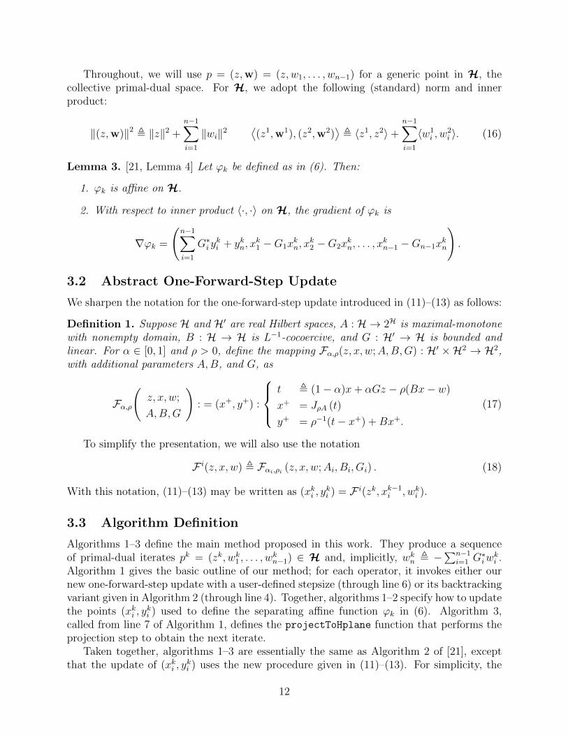
3.2 Abstract One-Forward-Step Update

We sharpen the notation for the one-forward-step update introduced in (11)–(13) as follows:

Definition 1. Suppose H and H′ are real Hilbert spaces, A : H → 2H is maximal-monotonewith nonempty domain, B : H → H is L−1-cocoercive, and G : H′ → H is bounded andlinear. For α ∈ [0, 1] and ρ > 0, define the mapping Fα,ρ(z, x, w;A,B,G) : H′ ×H2 → H2,with additional parameters A,B, and G, as

Fα,ρ

(z, x, w;

A,B,G

): = (x+, y+) :

t , (1− α)x+ αGz − ρ(Bx− w)

x+ = JρA (t)

y+ = ρ−1(t− x+) +Bx+.

(17)

To simplify the presentation, we will also use the notation

F i(z, x, w) , Fαi,ρi (z, x, w;Ai, Bi, Gi) . (18)

With this notation, (11)–(13) may be written as (xki , yki ) = F i(zk, xk−1i , wki ).

3.3 Algorithm Definition

Algorithms 1–3 define the main method proposed in this work. They produce a sequenceof primal-dual iterates pk = (zk, wk1 , . . . , w

kn−1) ∈ H and, implicitly, wkn , −

∑n−1i=1 G

∗iw

ki .

Algorithm 1 gives the basic outline of our method; for each operator, it invokes either ournew one-forward-step update with a user-defined stepsize (through line 6) or its backtrackingvariant given in Algorithm 2 (through line 4). Together, algorithms 1–2 specify how to updatethe points (xki , y

ki ) used to define the separating affine function ϕk in (6). Algorithm 3,

called from line 7 of Algorithm 1, defines the projectToHplane function that performs theprojection step to obtain the next iterate.

Taken together, algorithms 1–3 are essentially the same as Algorithm 2 of [21], exceptthat the update of (xki , y

ki ) uses the new procedure given in (11)–(13). For simplicity, the

12

Algorithm 1: One-Forward-Step Projective Splitting with Backtracking

Input: (z1,w1) ∈H, B ⊆ {1, . . . , n} (the operators requiring backtracking), γ > 0,δ ∈ (0, 1), and ρ. For i = 1, . . . , n: x0i ∈ Hi and 0 < αi ≤ 1. For i ∈ B: ρ0i > 0θi ∈ dom(Ai), wi ∈ Aiθi +Biθi, and y0i ∈ Aix0i +Bix

0i . For i /∈ B: ρi > 0.

1 For i ∈ B set η0i = 02 for k = 1, 2, . . . do3 for i ∈ B do4 (xki , y

ki , ρ

ki , η

ki ) = backTrack(zk, xk−1i , wki , yk−1i , ρk−1i , ηk−1i ; i)

/* backTrack defined in Algorithm 2 */

5 for i /∈ B do6 (xki , y

ki ) = F i(zk, xk−1i , wki ) /* F i defined in (17)-(18) */

7 (πk, zk+1,wk+1) = projectToHplane(zk, wk, {xki , yki }ni=1)

/* projectToHplane defined in Algorithm 3 */

8 if πk = 0 then9 return zk+1

Algorithm 2: Backtracking procedure

Global Variables for Function: Gi, Ai, Bi, αi, θi, and wi for i ∈ B, δ and ρ.1 Function backTrack(z, x, w, y, ρ, η; i):

2 A = Ai, B = Bi, G = Gi, α = αi, θ = θi, w = wi3 ϕ = 〈Gz − x, y − w〉4 ρ = min{(1 + αη)ρ, ρ}5 Choose ρ1 ∈ [ρ, ρ]6 for j = 1, 2, . . . do7 (xj, yj) = Fα,ρj(z, x, w;A,B,G) /* F defined in (17) */

8 yj = ρ−1j ((1− α)x+ αGz − xj) + w

9 ϕ+j = 〈Gz − xj, yj − w〉

10 if ‖xj − θ‖ ≤ (1− α)‖x− θ‖+ α‖Gz − θ‖+ ρj‖w − w‖11 and ϕ+

j ≥ρj2α

(‖yj − w‖2 + α‖yj − w‖2) + (1− α)(ϕ− ρj

2α‖y − w‖2

)then

12 η = ‖yj − w‖2/‖yj − w‖213 return (xj, yj, ρj, η)

14 ρj+1 = δρj

algorithm also lacks the block-iterative and asynchronous features of [10, 17, 21], which weplan to combine with algorithms 1–3 in a follow-up paper.

The computations in projectToHplane are all straightforward and of relatively low com-plexity. They consist of matrix multiplies by Gi, inner products, norms, and sums of scalars.In particular, there are no potentially difficult minimization problems involved. If Gi = Iand Hi = Rd for i = 1, . . . , n, then the computational complexity of projectToHplane is

13

Algorithm 3: Projection Update

Global Variables for Function: Gi for i = 1, . . . , n− 1, and γ.1 Function projectToHplane(z,w, {xi, yi}ni=1):2 ui = xi −Gixn, i = 1, . . . , n− 1,

3 v =∑n−1

i=1 G∗i yi + yn

4 π = ‖u‖2 + γ−1‖v‖25 if π > 0 then

6 ϕ(p) = 〈z, v〉+∑n−1

i=1 〈wi, ui〉 −∑n

i=1〈xi, yi〉7 τ = 1

π·max {0, ϕ(p)}

8 else9 return (0, xn, y1, . . . , yn−1)

10 z+ = z − γ−1τv11 w+

i = wi − τui, i = 1, . . . , n− 1,

12 w+n = −

∑n−1i=1 G

∗iw

+i

13 return (π, z+,w+)

O(nd).

3.4 Algorithm Parameters

The method allows two ways to select the stepsizes ρi. One may either choose them manuallyor invoke the backTrack procedure. If one decides to select the stepsizes manually, the upperbound condition ρi ≤ 2(1−αi)/Li is required whenever Li > 0. However, it may be difficultto ensure that this condition is satisfied when the cocoercivity constant is hard to estimate.The global cocoercivity constant Li may also be conservative in parts of the domain ofBi, leading to unnecessarily small stepsizes in some cases. We developed the backtrackinglinesearch technique for these reasons. The set B holds the indices of operators for whichbacktracking is to be used.

For a trial stepsize ρj, Algorithm 2 generates candidate points (xj, yj) using the single-forward-step procedure of (17). For these candidates, Algorithm 2 checks two conditionson lines 10–11. If both of these inequalities are satisfied, then backtracking terminates andreturns the successful candidate points. If either condition is not satisfied, the stepsize isreduced by the factor δ ∈ (0, 1) and the process is repeated. These two conditions arise inthe analysis in Section 5.

The parameter ρ is a global upper bound on the stepsizes (both backtracked and fixed)and must be chosen to satisfy Assumption 2. In backTrack, one must choose an initial trialstepsize within a specified interval (line 5 of Algorithm 2). This interval arises in the analysis(see lemmas 16 and 17). Written in terms of the parameters passed into backTrack in thecall on line 4 of Algorithm 1, and assuming the global upper bound ρ is sufficiently large tonot be active on line 5, the interval is[

ρki ,

(1 + αi

‖yki − wki ‖‖yki − wki ‖

)ρki

].

14

An obvious choice is to set the initial stepsize to be at the upper limit of the interval. Inpractice we have observed that ‖yki − wki ‖ and ‖yki − wki ‖ tend to be approximately equal,so this allows for an increase in the trial stepsize by up to a factor of approximately 1 + αiover the previous stepsize.

Note that backTrack returns the chosen stepsize ρj as well as the quantity η which areneeded to compute the available interval in the call to backTrack during the next iteration.

In the analysis it will be convenient to let ρ(i,k) be the initial trial stepsize chosen duringiteration k of Algorithm 1, when backTrack has been called through line 4 for some i ∈ B.

We call the stepsize returned by backTrack ρki . Assuming that backTrack always termi-nates finitely (which we will show to be the case), we may write for i ∈ B

(xki , yki ) = Fαi, ρki

(zk, xk−1i , wki ;Ai, Bi, Gi)

The only difference between the update for i ∈ B on line 6 and this update for i /∈ B is thatin the former, the stepsize ρki is discovered by backtracking, while in the latter it is directlyuser-supplied.

The backTrack procedure computes several auxiliary quantities used to check the twobacktracking termination conditions. The point yj is calculated to be the same as y given inDefinition 2. The quantity ϕ+

j = 〈Gz−xj, yj−w〉 is the value of ϕi,k(zk, wki ) corresponding to

the candidate points (xj, yj). The quantity ϕ computed on line 3 is equal to ϕi,k−1(zk, wki ) =

〈Gizk−xk−1i , yk−1i −wki 〉. Typically, we want ϕ+

j to be as large as possible to get a bigger cutwith the separating hyperplane, but the condition checked on line 11 will ultimately sufficeto prove convergence.

Algorithm 1 has several additional parameters.

(θi, wi) these are used in the backtracking procedure for i ∈ B. An obvious choice whichwe used in our numerical experiments was (θi, wi) = (x0i , y

0i ), i.e. the initial point.

γ > 0: allows for the projection to be performed using a slightly more general primal-dualmetric than (16). In effect, this parameter changes the relative size of the primal anddual updates in lines 10–11 of Algorithm 3. As γ increases, a smaller step is taken inthe primal and a larger step in the dual. As γ decreases, a smaller step is taken inthe dual update and a larger step is taken in the primal. See [19, Sec. 5.1] and [18,Sec. 4.1] for more details.

In Algorithm 1, the averaging parameters αi and user-selected stepsizes ρi are fixed acrossall iterations. In the preprint version of this paper [24], we instead allow these parameters tovary by iteration, subject to certain restrictions. Doing so complicates the notation and theanalysis, so for relative simplicity we consider only fixed values of these parameter here. Thissimplification also accords with the parameter choices in our computational tests below. Forthe full, more complicated analysis, please refer to [24].

As written, Algorithm 1 is not as efficient as it could be. On the surface, it seems thatwe need to recompute Bix

k−1i in order to evaluate F on line 6. However, Bix

k−1i was already

computed in the previous iteration and can obviously be reused, so only one evaluation ofBi is needed per iteration. Similarly, within backTrack, each invocation of F on line 7 mayreuse the quantity Bx = Bix

k−1i which was computed in the previous iteration of Algorithm

15

1. Thus, each iteration of the loop within backTrack requires one new evaluation of B, tocompute Bxj within F .

We now precisely state our stepsize assumption for the manually chosen stepsizes, as wellas the stepsize upper bound ρ.

Assumption 2. For i /∈ B: If Li > 0, then 0 < ρi ≤ 2(1 − αi)/Li, otherwise ρi > 0. Theparameter ρ must satisfy

ρ ≥ max

{maxi∈B

ρ0i ,maxi/∈B

ρi

}. (19)

Note that if Li > 0, Assumption 2 effectively limits αi to be strictly less than 1, otherwisethe stepsize ρi would be forced to 0, which is prohibited. In this case αi must be chosen in(0, 1). On the other hand, if Li = 0, there is no constraint on ρi other than that it is positiveand nonzero, and in this case αi may be chosen in (0, 1].

3.5 Separator-Projector Properties

Lemma 4 details the key results for Algorithm 1 that stem from it being a seperator-projectoralgorithm. While these properties alone do not guarantee convergence, they are importantto all of the arguments that follow.

Lemma 4. Suppose that Assumption 1 holds. Then for Algorithm 1

1. The sequence {pk} = {(zk, wk1 , . . . , wkn−1)} is bounded.

2. If the algorithm never terminates via line 9, pk−pk+1 → 0. Furthermore zk−zk−1 → 0and wki − wk−1i → 0 for i = 1, . . . n.

3. If the algorithm never terminates via line 9 and ‖∇ϕk‖ remains bounded for all k ≥ 1,then lim supk→∞ ϕk(p

k) ≤ 0.

Proof. Parts 1–2 are proved in lemmas 2 and 6 of [21]. Part 3 can be found in Part 1 ofthe proof of Theorem 1 in [21]. The analysis in [21] uses a different procedure to constructthe pairs (xki , y

ki ), but the result is generic and not dependent on that particular procedure.

Note also that [21] establishes the results in a more general setting allowing asynchrony andblock-iterativeness, which we do not analyze here.

4 The Special Case n = 1

Before starting the analysis, we consider the important special case n = 1. In this case, wehave by assumption that G1 = I, wk1 = 0, and we are solving the problem 0 ∈ Az+Bz, whereboth operators are maximal monotone and B is L−1-cocoercive. In this case, Algorithm 1reduces to a method which is similar to FB. Let xk , xk1, yk , yk1 , α , α1, and ρ , ρ1.

16

Assuming for simplicity that B = {∅}, meaning backtracking is not being used, then theupdates carried out by the algorithm are

xk = JρA((1− α)xk−1 + αzk − ρBxk−1

)(20)

yk = Bxk +1

ρ

((1− α)xk−1 + αzk − ρBxk−1 − xk

)zk+1 = zk − τ kyk, where τ k =

max{〈zk − xk, yk〉, 0}‖yk‖2

.

If α = 0, then for all k ≥ 2, the iterates computed in (20) reduce simply to

xk = JρA(xk−1 − ρBxk−1

)which is exactly FB. However, α = 0 is not allowed in our analysis. Thus, FB is a forbiddenboundary case which may be approached by setting α arbitrarily close to 0. As α approaches0, the stepsize constraint ρ ≤ 2(1−α)/L approaches the classical stepsize constraint for FB:ρ ≤ 2/L − ε for some arbitrarily small constant ε > 0. A potential benefit of Algorithm 1over FB in the n = 1 case is that it does allow for backtracking when L is unknown or onlya conservative estimate is available.

5 Main Proof

The core of the proof strategy will be to establish (21) below. If this can be done, then weakconvergence to a solution follows from part 3 of Theorem 1 in [21].

Lemma 5. Suppose Assumption 1 holds and Algorithm 1 produces an infinite sequence ofiterations without terminating via Line 9. If

(∀i = 1, . . . , n) : yki − wki → 0 and Gizk − xki → 0, (21)

then there exists (z,w) ∈ S such that (zk,wk) ⇀ (z,w). Furthermore, we also have xki ⇀Giz and yki ⇀ wi for all i = 1, . . . , n− 1, xkn ⇀ z, and ykn ⇀ −

∑n−1i=1 G

∗iwi.

Proof. Equivalent to part 3 of the proof of Theorem 1 in [21].

Lemma 5 can be intuitively understood as follows. If we define, for all k ≥ 1,

εk = maxi=1,...,n

{max

{‖yki − wki ‖, ‖Giz

k − xki ‖}}

,

then (21) is equivalent to saying that εk → 0. For all k ≥ 1, we have (xki , yki ) ∈ graTi. If

εk = 0, then wki = yki ∈ Tixki = TiGizk and since

∑ni=1G

∗iw

ki = 0, it follows that (zk,wk) ∈ S

and zk solves (3). Thus εk can be thought of as the “residual” of the algorithm whichmeasures how far it is from finding a point in S and a solution to (3). In finite dimension,it is straightforward to show that if εk → 0, (zk,wk) must converge to some element of S.This can be done using Fejer monotonicity [4, Theorem 5.5] combined with the fact thatthe graph of a maximal-monotone operator in a finite-dimensional Hilbert space is closed [4,

17

Proposition 20.38]. However in the general Hilbert space setting the proof is more delicate,since the graph of a maximal-monotone operator is not in-general closed in the weak-to-weak topology [4, Example 20.39]. Nevertheless the overall result was established in thegeneral Hilbert space setting in part 3 of Theorem 1 of [21], which is itself an instance of [1,Proposition 2.4] (see also [4, Proposition 26.5]). An arguably more transparent proof can befound in [16] (this proof is only for the case n = 2, but it can be extended).

In order to establish (21), we start by establishing certain contractive and “ascent” prop-erties for the mapping F , and also show that the backtracking procedure terminates finitely.Then, we prove the boundedness of xki and yki , in turn yielding the boundedness of the gradi-ents ∇ϕk and hence the result that lim supk→∞{ϕk(pk)} ≤ 0 by Lemma 4. Next we establisha “Lyapunov-like” recursion for ϕi,k(z

k, wki ), relating ϕi,k(zk, wki ) to ϕi,k−1(z

k−1, wk−1i ). Even-tually this result will allow us to establish that lim infk ϕk(p

k) ≥ 0 and hence that ϕk(pk)→ 0,

which will in turn allow an argument that yki − wki → 0. The proof that Gizk − xki → 0 will

then follow fairly elementary arguments.The primary innovations of the upcoming proof are the ascent lemma and the way that

it is used in Lemma 18 to establish ϕk(pk) → 0 and yki − wki → 0. This technique is a

significant deviation from previous analyses in the projective splitting family. In previouswork, the strategy was to show that ϕi,k(z

k, wki ) ≥ C max{‖Gizk − xki ‖2, ‖yki − wki ‖2} for a

constant C > 0, which may be combined with lim supϕk(pk) ≤ 0 to imply (21). In contrast,

in the algorithm of this paper we cannot establish such a result and in fact ϕi,k(zk, wki ) may

be negative. Instead, we relate ϕk(pk) to ϕk−1(p

k−1) to show that the separation improvesat each iteration in a way which still leads to overall convergence.

5.1 Some Basic Results

We begin by stating three elementary results on sequences, which may be found in [36], anda basic, well known nonexpansivity property for forward steps with cocoercive operators.

Lemma 6. [36, Lemma 1, Ch. 2] Suppose that ak ≥ 0 for all k ≥ 1, b ≥ 0, 0 ≤ τ < 1, andak+1 ≤ τak + b for all k ≥ 1. Then {ak} is a bounded sequence.

Lemma 7. [36, Lemma 3, Ch. 2] Suppose that ak ≥ 0, bk ≥ 0 for all k ≥ 1, bk → 0, andthere is some 0 ≤ τ < 1 such that ak+1 ≤ τak + bk for all k ≥ 1. Then ak → 0.

Lemma 8. Suppose that 0 ≤ τ < 1 and {rk}, {bk} are sequences in R with the propertiesbk → 0 and rk+1 ≥ τrk + bk for all k ≥ 1. Then lim infk→∞{rk} ≥ 0.

Proof. Negating the assumed inequality yields −rk+1 ≤ τ(−rk)− bk. Applying [36, Lemma3, Ch. 2] then yields lim sup{−rk} ≤ 0.

Lemma 9. Suppose B is L−1-cocoercive and 0 ≤ ρ ≤ 2/L. Then for all x, y ∈ dom(B)

‖x− y − ρ(Bx−By)‖ ≤ ‖x− y‖. (22)

Proof. Squaring the left hand side of (22) yields

‖x− y − ρ(Bx−By)‖2 = ‖x− y‖2 − 2ρ〈x− y,Bx−By〉+ ρ2‖Bx−By‖2

≤ ‖x− y‖2 − 2ρ

L‖Bx−By‖2 + ρ2‖Bx−By‖2

≤ ‖x− y‖2.

18

5.2 A Contractive Result

We begin the main proof with a result on the one-forward-step mapping: F from Definition1. The following lemma will ultimately be used to show that the iterates remain bounded.

Lemma 10. Suppose (x+, y+) = Fα,ρ(z, x, w;A,B,G), where Fα,ρ is given in Definition 1.Recall that B is L−1-cocoercive. If L = 0 or ρ ≤ 2(1− α)/L, then

‖x+ − θ‖ ≤ (1− α)‖x− θ‖+ α‖Gz − θ‖+ ρ ‖w − w‖ (23)

for any θ ∈ dom(A) and w ∈ Aθ +Bθ.

Proof. Select any θ ∈ dom(A) and w ∈ Aθ + Bθ. Let a = w − Bθ ∈ Aθ. It followsimmediately from (4) that

θ = JρA(θ + ρa). (24)

Therefore, (17) and (24) yield

‖x+ − θ‖ =∥∥∥JρA((1− α)x+ αGz − ρ(Bx− w)

)− JρA(θ + ρa)

∥∥∥(a)

≤∥∥∥(1− α)x+ αGz − ρ(Bx− w)− θ − ρa

∥∥∥(b)=

∥∥∥∥(1− α)

(x− θ − ρ

1− α

(Bx−Bθ

))+ α(Gz − θ) + ρ

(w − a−Bθ

)∥∥∥∥(c)

≤ (1− α)

∥∥∥∥x− θ − ρ

1− α

(Bx−Bθ

)∥∥∥∥+ α‖Gz − θ‖+ ρ∥∥∥w − (a+Bθ)

∥∥∥ (25)

(d)

≤ (1− α)‖x− θ‖+ α‖Gz − θ‖+ ρ ‖w − w‖ .

To obtain (a), one uses the nonexpansivity of the resolvent [4, Prop. 23.8(ii)]. To obtain (b),one regroups terms and adds and subtracts Bθ. Then (c) follows from the triangle inequality.Finally we consider (d): If L > 0, apply Lemma 9 to the first term on the right-hand side of(25) with the stepsize ρ/(1− α) which by assumption satisfies

ρ

1− α≤ 2

L

by Assumption 2. Alternatively, if L = 0, implying that B is a constant-valued operator,then Bx = Bθ and (d) is just an equality.

We now prove the key “ascent lemma”. It shows that, while the one-forward-step updateis not guaranteed to find a separating hyperplane at each iteration, it does make a certainkind of progress toward separation.

19

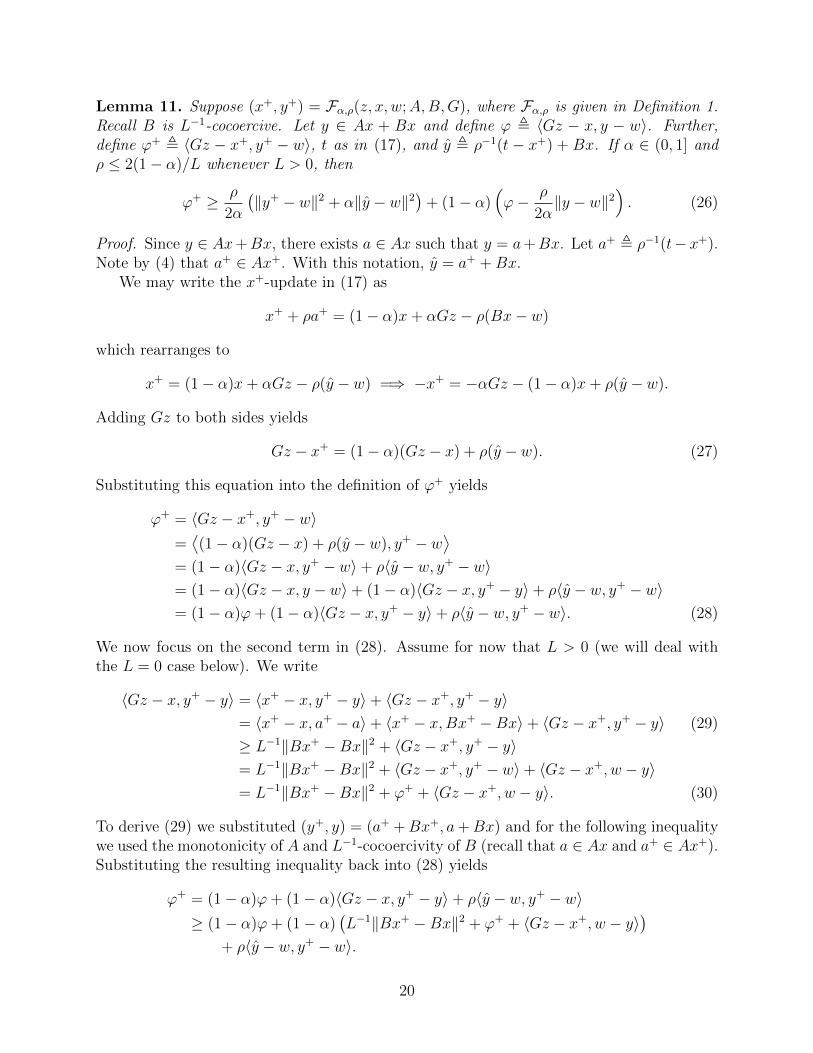
Lemma 11. Suppose (x+, y+) = Fα,ρ(z, x, w;A,B,G), where Fα,ρ is given in Definition 1.Recall B is L−1-cocoercive. Let y ∈ Ax + Bx and define ϕ , 〈Gz − x, y − w〉. Further,define ϕ+ , 〈Gz − x+, y+ − w〉, t as in (17), and y , ρ−1(t − x+) + Bx. If α ∈ (0, 1] andρ ≤ 2(1− α)/L whenever L > 0, then

ϕ+ ≥ ρ

2α

(‖y+ − w‖2 + α‖y − w‖2

)+ (1− α)

(ϕ− ρ

2α‖y − w‖2

). (26)

Proof. Since y ∈ Ax+Bx, there exists a ∈ Ax such that y = a+Bx. Let a+ , ρ−1(t−x+).Note by (4) that a+ ∈ Ax+. With this notation, y = a+ +Bx.

We may write the x+-update in (17) as

x+ + ρa+ = (1− α)x+ αGz − ρ(Bx− w)

which rearranges to

x+ = (1− α)x+ αGz − ρ(y − w) =⇒ −x+ = −αGz − (1− α)x+ ρ(y − w).

Adding Gz to both sides yields

Gz − x+ = (1− α)(Gz − x) + ρ(y − w). (27)

Substituting this equation into the definition of ϕ+ yields

ϕ+ = 〈Gz − x+, y+ − w〉=⟨(1− α)(Gz − x) + ρ(y − w), y+ − w

⟩= (1− α)〈Gz − x, y+ − w〉+ ρ〈y − w, y+ − w〉= (1− α)〈Gz − x, y − w〉+ (1− α)〈Gz − x, y+ − y〉+ ρ〈y − w, y+ − w〉= (1− α)ϕ+ (1− α)〈Gz − x, y+ − y〉+ ρ〈y − w, y+ − w〉. (28)

We now focus on the second term in (28). Assume for now that L > 0 (we will deal withthe L = 0 case below). We write

〈Gz − x, y+ − y〉 = 〈x+ − x, y+ − y〉+ 〈Gz − x+, y+ − y〉= 〈x+ − x, a+ − a〉+ 〈x+ − x,Bx+ −Bx〉+ 〈Gz − x+, y+ − y〉 (29)

≥ L−1‖Bx+ −Bx‖2 + 〈Gz − x+, y+ − y〉= L−1‖Bx+ −Bx‖2 + 〈Gz − x+, y+ − w〉+ 〈Gz − x+, w − y〉= L−1‖Bx+ −Bx‖2 + ϕ+ + 〈Gz − x+, w − y〉. (30)

To derive (29) we substituted (y+, y) = (a+ +Bx+, a+Bx) and for the following inequalitywe used the monotonicity of A and L−1-cocoercivity of B (recall that a ∈ Ax and a+ ∈ Ax+).Substituting the resulting inequality back into (28) yields

ϕ+ = (1− α)ϕ+ (1− α)〈Gz − x, y+ − y〉+ ρ〈y − w, y+ − w〉≥ (1− α)ϕ+ (1− α)

(L−1‖Bx+ −Bx‖2 + ϕ+ + 〈Gz − x+, w − y〉

)+ ρ〈y − w, y+ − w〉.

20

Subtracting (1− α)ϕ+ from both sides of the above inequality produces

αϕ+ ≥ (1− α)(ϕ+ L−1‖Bx+ −Bx‖2 + 〈Gz − x+, w − y〉

)+ ρ〈y − w, y+ − w〉. (31)

Using (27) once again, this time to the third term on the right-hand side of (31), we write

〈Gz − x+, w − y〉 =⟨(1− α)(Gz − x) + ρ(y − w), w − y

⟩= (1− α)〈Gz − x,w − y〉+ ρ〈y − w,w − y〉= (α− 1)ϕ− ρ〈y − w, y − w〉. (32)

Substituting this equation back into (31) yields

αϕ+ ≥ (1− α)(αϕ+ L−1‖Bx+ −Bx‖2 − ρ〈y − w, y − w〉

)+ ρ〈y − w, y+ − w〉. (33)

We next use the identity 〈x1, x2〉 = 12‖x1‖2 + 1

2‖x2‖2 − 1

2‖x1 − x2‖2 on both inner products

in (33), as follows:

〈y − w, y − w〉 =1

2

(‖y − w‖2 + ‖y − w‖2 − ‖y − y‖2

)=

1

2

(‖y − w‖2 + ‖y − w‖2 − ‖a+ − a‖2

)(34)

and

〈y − w, y+ − w〉 =1

2

(‖y − w‖2 + ‖y+ − w‖2 − ‖y − y+‖2

)=

1

2

(‖y − w‖2 + ‖y+ − w‖2 − ‖Bx+ −Bx‖2

). (35)

Here we have used the identities

y − y = a+ +Bx− (a+Bx) = a+ − ay − y+ = a+ +Bx− (a+ +Bx+) = Bx−Bx+.

Using (34)–(35) in (33) yields

αϕ+ ≥ (1− α)(αϕ+ L−1‖Bx+ −Bx‖2 − ρ〈y − w, y − w〉

)+ ρ〈y − w, y+ − w〉

= (1− α)(αϕ+ L−1‖Bx+ −Bx‖2

)− ρ(1− α)

2

(‖y − w‖2 + ‖y − w‖2 − ‖a+ − a‖2

)+ρ

2

(‖y − w‖2 + ‖y+ − w‖2 − ‖Bx+ −Bx‖2

)= (1− α)

(αϕ− ρ

2‖y − w‖2 +

ρ

2‖a+ − a‖2

)+

(1− αL− ρ

2

)‖Bx+ −Bx‖2

+ρ

2

(‖y+ − w‖2 + α‖y − w‖2

).

Consider this last expression: since α ≤ 1, the coefficient (1− α)ρ/2 multiplying ‖a+ − a‖2is nonnegative. Furthermore, since ρ ≤ 2(1−α)/L, the coefficient multiplying ‖Bx+−Bx‖2

21

is positive. Therefore we may drop these two terms from the above inequality and divide byα to obtain (26).

Finally, we deal with the case in which L = 0, which implies that Bx = v for some v ∈ Hfor all x ∈ H. The main difference is that the ‖Bx+ − Bx‖2 terms are no longer presentsince Bx+ = Bx. The analysis is the same up to (28). In this case Bx+ = v so instead of(30) we may deduce from (29) that

〈Gz − x, y+ − y〉 ≥ ϕ+ + 〈Gz − x+, w − y〉.

Since Bx+ = Bx = v is constant we also have that

y = a+ +Bx = a+ + v = a+ +Bx+ = y+

Thus, instead of (31) in this case we have the simpler inequality

αϕ+ ≥ (1− α)(ϕ+ 〈Gz − x+, w − y〉

)+ ρ‖y+ − w‖2. (36)

The term 〈Gz−x+, w− y〉 in (36) is dealt with just as in (31), by substitution of (27). Thisstep now leads via (32) to

αϕ+ ≥ α(1− α)ϕ− ρ(1− α)〈y+ − w, y − w〉+ ρ‖y+ − w‖2.

Once again using 〈x1, x2〉 = 12‖x1‖2 + 1

2‖x2‖2 − 1

2‖x1 − x2‖2 on the second term on the

r.h.s. above yields

αϕ+ ≥ α(1− α)ϕ+ ρ‖y+ − w‖2 − ρ(1− α)

2

(‖y+ − w‖2 + ‖y − w‖2 − ‖y+ − y‖2

).

We can lower-bound the ‖y+ − y‖2 term by 0. Dividing through by α and rearranging, weobtain

ϕ+ ≥ ρ(1 + α)

2α‖y+ − w‖2 + (1− α)

(ϕ− ρ

2α‖y − w‖2

).

Since y+ = y in the L = 0 case, this is equivalent to (26).

5.3 Finite Termination of Backtracking

In all the following lemmas in sections 5.3 and 5.4 regarding algorithms 1–3, assumptions 1and 2 are in effect and will not be explicitly stated in each lemma. We start by proving thatbackTrack terminates in a finite number of iterations, and that the stepsizes it returns arebounded away from 0.

Lemma 12. For i ∈ B, Algorithm 2 terminates in a finite number of iterations for allk ≥ 1. There exists ρ

i> 0 such that ρki ≥ ρ

ifor all k ≥ 1, where ρki is the stepsize returned

by Algorithm 2 on line 4. Furthermore ρki ≤ ρ for all k ≥ 1.

22

Proof. Assume we are at iteration k ≥ 1 in Algorithm 1 and backTrack has been calledthrough line 4 for some i ∈ B. The internal variables within backTrack are defined in termsof the variables passed from Algorithm 1 as follows: z = zk, x = xk−1i , w = wki , y = yk−1i ,

ρ = ρk−1i and η = ηk−1i . Furthermore α = αi, θ = θi, w = wi, A = Ai, B = Bi, andG = Gi. The calculation on line 3 of Algorithm 2 yields ϕ = ϕi,k−1(z

k, wki ). In the followingargument, we mostly refer to the internal name of the variables within backTrack withoutexplicitly making the above substitutions. With that in mind, let L = Li be the cocoercivityconstant of B = Bi.

Recall that ρ(i,k) is the initial trial stepsize ρ1 chosen on line 5 of backTrack. We mustestablish that the interval on line 5 is always nonempty and so a valid initial stepsize can bechosen. Since ηα ≥ 0, this will be true if ρ ≥ ρ = ρk−1i , which we will prove by induction.Note that by Assumption 2, ρ ≥ ρ0i for all i ∈ B. Therefore for k = 1, ρ ≥ ρ = ρ0i . We willprove the induction step below.

Observe that backtracking terminates via line 13 if two conditions are met. The firstcondition,

‖xj − θ‖ ≤ (1− α)‖x− θ‖+ α‖Gz − θ‖+ ρj‖w − w‖, (37)

is identical to (23) of Lemma 10, with xj and ρj respectively in place of x+ and ρ. The

initialization step of Algorithm 2 provides us with w ∈ Aθ + Bθ for some θ ∈ dom(A).Furthermore, since

(xj, yj) = Fα,ρj(z, x, w;A,B,G),

the findings of Lemma 10 may be applied. In particular, if L > 0 and ρj ≤ 2(1−α)/L, then(37) will be met. Alternatively, if L = 0, (37) will hold for any value of the stepsize ρj > 0.

Next, consider the second termination condition,

ϕ+j ≥

ρj2α

(‖yj − w‖2 + α‖yj − w‖2

)+ (1− α)

(ϕ− ρj

2α‖y − w‖2

). (38)

This relation is identical to (26) of Lemma 11, with (yj, yj, ρj) in place of (y+, y, ρ). However,to apply the lemma we must show that y = yk−1i ∈ Axk−1i +Bxk−1i = Ax+Bx. We will alsoprove this by induction.

For k = 1, y = yk−1i ∈ Axk−1i + Bxk−1i = Ax + Bx holds by the initialization step ofAlgorithm 1. Now assume that at iteration k ≥ 2 it holds that y = yk−1i ∈ Axk−1i +Bxk−1i =Ax + Bx and furthermore that ρ ≥ ρ = ρk−1i , therefore the interval on line 5 is nonempty.We may then apply the findings of Lemma 11 to conclude that if L > 0 and ρj ≤ 2(1−α)/L,then condition (38) is satisfied. Or, if L = 0, condition (38) is satisfied for any ρj > 0.

Combining the above observations, we conclude that if L > 0 and ρj ≤ 2(1 − α)/L,backtracking will terminate for that iteration j of backTrack via line 13. Or, if L = 0, itwill terminate in the first iteration of backTrack. The stepsize decrement condition on line14 of the backtracking procedure implies that ρj ≤ 2(1− α)/L will eventually hold for largeenough j, and hence that the two backtracking termination conditions must eventually hold.

Let j∗ ≥ 1 be the iteration at which backtracking terminates when called for operatori at iteration k of Algorithm 1. For the pair (xki , y

ki ) returned by backTrack on line 4 of

23

Algorithm 1, we may write

(xki , yki ) = (xj∗ , yj∗) = Fα,ρj∗ (z, x, w;A,B,G) = Fαk

i ,ρki(zk, xk−1i , wki ;Ai, Bi, Gi).

Thus, by the definition of F in (17), yki ∈ Aixki +Bixki . Therefore, induction establishes that

yki ∈ Aixki +Bixki holds for all k ≥ 1.

Now the returned stepsize must satisfy ρki = ρj∗ ≤ ρ(i,k) ≤ ρ. In the next iteration,ρ = ρki ≤ ρ. Thus we have also established by induction that ρ ≥ ρ = ρki and therefore thatthe interval on line 5 is nonempty for all iterations k ≥ 1. Finally, we now also infer byinduction that backTrack terminates in a finite number of iterations for all k ≥ 1 and i ∈ B.

Now ρ(i,k) must be chosen in the range

ρ(i,k) ∈[ρk−1i ,min

{(1 + αiη

k−1i )ρk−1i , ρ

}].

Since we have established that this interval remains nonempty, it holds trivially that ρ(i,k) ≥ρk−1i . For all k ≥ 1 and i ∈ B, the returned stepsize ρki = ρj∗ must satisfy

(∀ i : Li > 0) : ρki ≥ min

{ρ(i,k),

2δ(1− αi)Li

}(39)

(∀ i : Li = 0) : ρki = ρ(i,k).

Therefore for all k ≥ 1 and all i ∈ B such that Li > 0, one has

ρki ≥ min

{ρk−1i ,

2δ(1− αi)Li

}≥ min

{ρ1i ,

2δ(1− αi)Li

}≥ min

{ρ0i ,

2δ(1− αi)Li

}, ρ

i> 0,

where the first inequality uses (39) and ρ(i,k) ≥ ρk−1i , the second inequality recurses, and thefinal inequality is just (39) for k = 1. If Li = 0, the argument is simply

ρki = ρ(i,k) ≥ ρk−1i = ρ(i,k−1) ≥ . . . ≥ ρ1i = ρ(i,1) = ρ0i , ρi> 0.

5.4 Boundedness Results and their Direct Consequences

Lemma 13. For all i = 1, . . . , n, the sequences {xki } and {yki } are bounded.

Proof. To prove this, we first establish that for i = 1, . . . , n and k ≥ 1

‖xki − θi‖ ≤ (1− αi)‖xk−1i − θi‖+ αi‖Gizk − θi‖+ ρ

∥∥wki − wi∥∥ (40)

For i ∈ B, Lemma 12 establishes that backTrack terminates for finite j ≥ 1 for all k ≥ 1.For fixed k ≥ 1 and i ∈ B, let j∗ ≥ 1 be the iteration of backTrack that terminates. Attermination, the following condition is satisfied via line 10:

‖xj∗ − θ‖ ≤ (1− α)‖x− θ‖+ α‖Gz − θ‖+ ρj∗‖w − w‖.

24

Into this inequality, now substitute in the following variables from Algorithm 1, as passed toand from backTrack: xki = xj∗ , θi = θ, αi = α, xk−1i = x, Gi = G, zk = z, ρki = ρj∗ , wki = w,and wi = w. Further noting that ρki ≤ ρ, the result is (40).

For i /∈ B, we note that line 6 of Algorithm 1 reads as

(xki , yki ) = Fαi,ρi(z

k, xk−1i , wki ;Ai, Bi, Gi)

and since Assumption 2 holds, we may apply Lemma 10. Further noting that by Assumption2 ρi ≤ ρ we arrive at yield (40).

Since {zk}, and {wki } are bounded by Lemma 4 and ‖Gi‖ is bounded by Assumption 1,boundedness of {xki } now follows by applying Lemma 6 with τ = 1− αi < 1 to (40).

Next, boundedness of Bixki follows from the continuity of Bi. Since Lemma 12 established

that backTrack terminates in a finite number of iterations we have for any k ≥ 2 that

(xki , yki ) = Fαk

i ,ρki(zk, xk−1i , wki ;Ai, Bi, Gi)

where for i /∈ B ρki , ρi. Expanding the y+-update in the definition of F in (17), we maywrite

yki = (ρki )−1 ((1− αi)xk−1i + αiGiz

k − ρki (Bixk−1i − wki )− xki

)+Bxki .

Since Gi, zk, and wki are bounded, for i ∈ B ρki ≤ ρ, and ρki ≥ ρ

i(using Lemma 12 for i ∈ B),

and for i /∈ B ρki = ρi is constant, we conclude that yki remains bounded.

With {xki } and {yki } bounded for all i = 1, . . . , n, the boundedness of ∇ϕk follows imme-diately:

Lemma 14. The sequence {∇ϕk} is bounded. If Algorithm 1 never terminates via line 9,lim supk→∞ ϕk(p

k) ≤ 0.

Proof. By Lemma 3, ∇zϕk =∑n

i=1G∗i yki , which is bounded since each Gi is bounded by

assumption and each {yki } is bounded by Lemma 13. Furthermore, ∇wiϕk = xki − Gix

kn is

bounded using the same two lemmas. That lim supk→∞ ϕk(pk) ≤ 0 then immediately follows

from Lemma 4(3).

Using the boundedness of {xki } and {yki }, we can next derive the following simple boundrelating ϕi,k−1(z

k, wki ) to ϕi,k−1(zk−1, wk−1i ):

Lemma 15. There exists M1,M2 ≥ 0 such that for all k ≥ 2 and i = 1, . . . , n,

ϕi,k−1(zk, wki ) ≥ ϕi,k−1(z

k−1, wk−1i )−M1‖wki − wk−1i ‖ −M2‖Gi‖‖zk − zk−1‖.

Proof. For each i ∈ {1, . . . , n}, let M1,i,M2,i ≥ 0 be respective bounds on{‖Giz

k−1−xk−1i ‖}

and{‖yk−1i −wki ‖

}, which must exist by Lemma 4, the boundedness of {xki } and {yki }, and

25

the boundedness of Gi. Let M1 = maxi=1,...,m{M1,i} and M2 = maxi=1,...,m{M2,i}. Then, forany k ≥ 2 and i ∈ {1, . . . , n}, we may write

ϕi,k−1(zk, wki ) = 〈Giz

k − xk−1i , yk−1i − wki 〉= 〈Giz

k−1 − xk−1i , yk−1i − wki 〉+ 〈Gizk −Giz

k−1, yk−1i − wki 〉= 〈Giz

k−1 − xk−1i , yk−1i − wk−1i 〉+ 〈Gizk−1 − xk−1i , wk−1i − wki 〉

+ 〈Gizk −Giz

k−1, yk−1i − wki 〉≥ ϕi,k−1(z

k−1, wk−1i )−M1‖wki − wk−1i ‖ −M2‖Gi‖‖zk − zk−1‖,

where the last step uses the Cauchy-Schwarz inequality and the definitions of M1 and M2.

5.5 A Lyapunov-Like Recursion for the Hyperplane

We now establish a Lyapunov-like recursion for the hyperplane. For this purpose, we needtwo more definitions.

Definition 2. For all k ≥ 1, since Lemma 12 establishes that Algorithm 2 terminates in afinite number of iterations, we may write for i = 1, . . . , n:

(xki , yki ) = Fαi,ρki

(zk, xk−1i , wki ;Ai, Bi, Gi)

where for i /∈ B ρki = ρi are actually fixed. Using (4) and the x+-update in (17), there existsaki ∈ Aixki such that

xki + ρki aki = (1− αi)xk−1i + αiGiz

k − ρki (Bixk−1i − wki ).

Define yki , aki +Bixk−1i .

Definition 3. For i /∈ B we will use ρki , ρi, even though these stepsizes are fixed, so thatwe can use the same statements as for i ∈ B. Similarly we will use ρ

i, ρi for i /∈ B.

Lemma 16. For all k ≥ 1, and i = 1, . . . , n

ρk+1i

αi‖yki − wki ‖2 ≤

ρkiαi

(‖yki − wki ‖2 + αi‖yki − wki ‖2

). (41)

Proof. For i ∈ B, recall that ρ(i,k) is the initial trial stepsize chose on line 5 of backTrack atiteration k for some i ∈ B. The condition on line 5 of backTrack guarantees that

ρ(i,k+1) ≤ ρki

(1 + αi

‖yki − wki ‖2

‖yki − wki ‖2

).

Multiplying through by α−1i ‖yki − wki ‖2 and noting that ρk+1i ≤ ρ(i,k+1) proves the lemma.

For i /∈ B the expression holds trivially because ρk+1i = ρki = ρi.

26

Lemma 17. For all k ≥ 2 and i = 1, . . . , n,

ϕi,k(zk, wki )−

ρki2αi

(‖yki − wki ‖2 + αi‖yki − wki ‖2

)≥ (1− αi)

(ϕi,k−1(z

k, wki )−ρki2αi‖yk−1i − wki ‖2

)(42)

and

ϕi,k(zk, wki )−

ρk+1i

2αi‖yki − wki ‖2 ≥ (1− αi)

(ϕi,k−1(z

k, wki )−ρki2αi‖yk−1i − wki ‖2

). (43)

Proof. Take any i ∈ B. Lemma 12 guarantees the finite termination of backTrack. Nowconsider the backtracking termination condition

ϕ+j ≥

ρj2α

(‖yj − w‖2 + α‖yj − w‖2

)+ (1− α)

(ϕ− ρj

2α‖y − w‖2

).

Fix some k ≥ 2, and let j∗ ≥ 1 be the iteration at which backTrack terminates. In theabove inequality, make the following substitutions for the internal variables of backTrack bythose passed in/out of the function: ϕi,k(z

k, xki ) = ϕ+j∗ , ρki = ρj∗ , αi = α, yki = yj, w

ki = w,

ϕi,k−1(zk, wki ) = ϕ. Furthermore, yki = yj∗ where yki is defined in Definition 2. Together,

these substitutions yield (42). We can then apply Lemma 16 to get (43).Now take any i ∈ {1, . . . , n}\B. From line 6 of Algorithm 1, Assumption 2, and Lemma

11, we directly deduce (42). Combining this relation with (41) we obtain (43).

5.6 Finishing the Proof

We now work toward establishing the conditions of Lemma 5. Unless otherwise specified,we henceforth assume that Algorithm 1 runs indefinitely and does not terminate at line 9.Termination at line 9 is dealt with in Theorem 1 to come.

Lemma 18. For all i = 1, . . . , n, we have yki − wki → 0 and ϕk(pk)→ 0.

Proof. Fix any i ∈ {1, . . . , n}. First, note that for all k ≥ 2,

‖yk−1i − wki ‖2 = ‖yk−1i − wk−1i ‖2 + 2〈yk−1i − wk−1i , wk−1i − wki 〉+ ‖wk−1i − wki ‖2

≤ ‖yk−1i − wk−1i ‖2 +M3‖wki − wk−1i ‖+ ‖wki − wk−1i ‖2

= ‖yk−1i − wk−1i ‖2 + dki , (44)

where dki , M3‖wki − wk−1i ‖ + ‖wki − wk−1i ‖2 and M3 ≥ 0 is a bound on 2‖yk−1i − wk−1i ‖,which must exist because both {yki } and {wki } are bounded by lemmas 4 and 13. Note thatdki → 0 as a consequence of Lemma 4.

Second, recall Lemma 15, which states that there exists M1,M2 ≥ 0 such that for allk ≥ 2,

ϕi,k−1(zk, wki ) ≥ ϕi,k−1(z

k−1, wk−1i )−M1‖wk−1i − wki ‖ −M2‖Gi‖‖zk − zk−1‖. (45)

27

Now let, for all k ≥ 1,

rki , ϕi,k(zk, wki )−

ρk+1i

2αi‖yki − wki ‖2, (46)

so that

n∑i=1

rki = ϕk(pk)−

n∑i=1

ρk+1i

2αi‖yki − wki ‖2. (47)

Using (44) and (45) in (43) yields

(∀k ≥ 2) : rki ≥ (1− αi)rk−1i + eki (48)

where

eki , −(1− αi)(ρki2αi

dki +M1‖wk−1i − wki ‖+M2‖Gi‖‖zk − zk−1‖). (49)

Note that ρki is bounded, 0 < αi ≤ 1, ‖Gi‖ is finite, ‖zk−zk−1‖ → 0 and ‖wki −wk−1i ‖ → 0by Lemma 4, and dki → 0. Thus eki → 0.

Since 0 < αi ≤ 1, we may apply Lemma 8 to (48) with τ = 1 − αi < 1, which yieldslim infk→∞{rki } ≥ 0. Therefore

lim infk→∞

n∑i=1

rki ≥n∑i=1

lim infk→∞

rki ≥ 0. (50)

On the other hand, lim supk→∞ ϕk(pk) ≤ 0 by Lemma 14. Therefore, using (47) and (50),

0 ≤ lim infk→∞

n∑i=1

rki = lim infk→∞

{ϕk(p

k)−n∑i=1

ρk+1i

2αi‖yki − wki ‖2

}≤ lim inf

k→∞ϕk(p

k) ≤ lim supk→∞

ϕk(pk) ≤ 0.

Therefore limk→∞{ϕk(p

k)}

= 0. Consider any i ∈ {1, . . . , n}. Combining limk→∞{ϕk(p

k)}

=0 with lim infk→∞

∑ni=1 r

ki ≥ 0, we have

lim supk→∞

{(ρk+1i /αi)‖yki − wki ‖2

}≤ 0 ⇒ ρk+1

i ‖yki − wki ‖2 → 0.

Since ρki ≥ ρi> 0 (using Lemma 12 for i ∈ B) we conclude that yki − wki → 0.

We have already proved the first requirement of Lemma 5, that yki − wki → 0 for alli ∈ {1, . . . , n}. We now work to establish the second requirement, that Giz

k − xki → 0. Inthe upcoming lemmas we continue to use the quantity yki which is given in Definition 2.

Lemma 19. Recall {yki }k∈N from Definition 2. For all i = 1, . . . , n, yki − wki → 0.

28

Proof. Fix any k ≥ 1. For all i = 1, . . . , n, repeating (42) from Lemma 17, we have

ϕi,k(zk, wki ) ≥ (1− αi)

(ϕi,k−1(z

k, wki )−ρki2αi‖yk−1i − wki ‖2

)+

ρki2αi

(‖yki − wki ‖2 + αi‖yki − wki ‖2

)≥ (1− αi)rk−1i +

ρki2‖yki − wki ‖2 + eki

where we have used rki defined (46) along with (44)–(45) and eki is defined in (49). This isthe same argument used in Lemma 18, but now we apply (44)–(45) to (42), rather than (43),so that we can upper bound the ‖yki − wki ‖2 term. Summing over i = 1, . . . , n, yields

ϕk(pk) =

n∑i=1

ϕi,k(zk, wki ) ≥

n∑i=1

(1− αi)rk−1i +n∑i=1

ρki2‖yki − wki ‖2 +

n∑i=1

eki .

Since ϕk(pk) → 0, eki → 0, lim infk→∞{rki } ≥ 0, and ρki ≥ ρ

i> 0 for all k, the above

inequality implies that yki − wki → 0.

Lemma 20. For i = 1 . . . , n, xki − xk−1i → 0.

Proof. Fix i ∈ {1, . . . , n}. Using the definition of aki in Definition 2, we have for k ≥ 1 that

xki + ρki aki = (1− αi)xk−1i + αiGiz

k − ρki (Bixk−1i − wki ).

Using the definition of yki , also in Definition 2, this implies that

(∀k ≥ 1) : xki = (1− αi)xk−1i + αiGizk − ρki (yki − wki ), (51)

(∀k ≥ 2) : xk−1i = (1− αi)xk−2i + αiGizk−1 − ρk−1i (yk−1i − wk−1i ).

Subtracting the second of these equations from the first yields, for all k ≥ 2,

xki − xk−1i = (1− αi)(xk−1i − xk−2i ) + αi(Gizk −Giz

k−1)− ρki (yki − wki )+ ρk−1i (yk−1i − wk−1i )

Taking norms and using the triangle inequality yields, for all k ≥ 2, that

‖xki − xk−1i ‖ ≤ (1− αi) ‖xk−1i − xk−2i ‖+ eki (52)

whereeki = ‖Gi‖ ‖zki − zk−1i ‖+ ρki ‖yki − wki ‖+ ρk−1i ‖yk−1i − wk−1i ‖

Since ρki is bounded from above, eki → 0 using Lemma 19, the finiteness of ‖Gi‖, andLemma 4. Furthermore, αi > 0, so we may apply Lemma 7 to (52) to conclude thatxki − xk−1i → 0.

Lemma 21. For i = 1, . . . , n, Gizk − xki → 0.

29

Proof. Recalling (51), we first write

xki = (1− αi)xk−1i + αiGizk − ρki (yki − wki )

⇔ αi(Giz

k − xki)

= (1− αi)(xki − xk−1i ) + ρki (yki − wki ). (53)

Lemma 20 implies that the first term on the right-hand side of (53) converges to zero.Since {ρki } is bounded, Lemma 19 implies that the second term on the right-hand side alsoconverges to zero. Since αi > 0, we conclude that ‖Giz

k − xki ‖ → 0.

Finally, we can state our convergence result for Algorithm 1:

Theorem 1. Suppose that assumptions 1-2 hold. If Algorithm 1 terminates by reachingline 9, then its final iterate is a member of the extended solution set S. Otherwise, thesequence {(zk,wk)} generated by Algorithm 1 converges weakly to some point (z,w) in theextended solution set S of (2) defined in (5). Furthermore, xki ⇀ Giz and yki ⇀ wi for alli = 1, . . . , n− 1, xkn ⇀ z, and ykn ⇀ −

∑n−1i=1 G

∗iwi.

Proof. For the finite termination result we refer to Lemma 5 of [21]. Otherwise, lemmas 18and 21 imply that the hypotheses of Lemma 5, hold, and the result follows.

6 Numerical Experiments

All our numerical experiments were implemented in Python (using numpy and scipy) onan Intel Xeon workstation running Linux with 16 cores and 64 GB of RAM. The code isavailable via github at https://github.com/projective-splitting/coco. We restrictedour attention to algorithms with comparable features and benefits to our proposed method.Thus we only considered methods that:

1. Are first-order and “fully split” the problem (that is, separate the linear operators Gi

from the resolvent calculations, and use gradient-type steps for smooth functions),

2. Do not (either approximately or exactly) solve a linear system of equations at eachiteration or before the first iteration,

3. Avoid having to apply “smoothing” to nonsmooth operators,

4. Incorporate a backtracking linesearch in a manner that avoids the need for bounds onLipschitz or cocoercivity constants, and

5. Do not use iterative approximation of resolvents.

The last property we include for reasons of simplicity, while the rest contribute to makingalgorithms scalable and easy to apply. For a given application, there may of course beeffective algorithms which could have been considered but do not satisfy all of the aboverequirements. However, because of the general desirability of properties 1-4 and the relativesimplicity of algorithms with property 5, we only considered methods having all of them.

We compared this paper’s backtracking one-forward-step projective splitting algorithmgiven in Algorithm 1 (which we call ps1fbt) with the following methods:

30

• The two-forward-step projective splitting algorithm with backtracking we developedin [21] (ps2fbt). This method requires only Lipschitz continuity of single-valued op-erators, as opposed to cocoercivity.

• The adaptive three-operator splitting algorithm of [34] (ada3op) (where “adaptive” isused to mean “backtracking linesearch”); this method is a backtracking adaptation ofthe fixed-stepsize method proposed in [14]. This method requires Gi = I in problem (2)and hence can only be readily applied to two of the three test applications describedbelow.

• The backtracking linesearch variant of the Chambolle-Pock primal-dual splitting method[30] (cp-bt).

• The algorithm of [12]. This is essentially Tseng’s method applied to a product-space“monotone + skew” inclusion in the following way: Assume Tn is Lipschitz monotone,problem (3) is equivalent to finding p , (z, w1, . . . , wn−1) such that wi ∈ TiGiz (whichis equivalent to Giz ∈ T−1i wi) for i = 1, . . . , n − 1, and

∑n−1i=1 G

∗iwi = −Tnz. In other

words, we wish to solve 0 ∈ Ap+ Bp, where A and B are defined by

Ap = {0} × T−11 w1 × · · · × T−1n−1wn−1 (54)

Bp =

Tnz

0...

0

+

0 G∗1 G∗2 . . . G∗n−1−G1 0 . . . . . . 0

......

. . . . . ....

−Gn−1 0 . . . . . . 0

z

w1...

wn−1

. (55)

A is maximal monotone, while B is the sum of two Lipshitz monotone operators (thesecond being skew linear), and therefore also Lipschitz monotone. The algorithmin [12] is essentially Tseng’s forward-backward-forward method [40] applied to thisinclusion, using resolvent steps for A and forward steps for B. Thus, we call thismethod tseng-pd. In order to achieve good performance with tseng-pd we had toincorporate a diagonal preconditioner as proposed in [41].

• The recently proposed forward-reflected-backward method [31], applied to this sameprimal-dual inclusion 0 ∈ Ap+ Bp specified by (54)-(55). We call this method frb-pd.

Recently there have been several stochastic extensions of ada3op and cp-bt [42, 43, 33].The method of [43] requires estimates of the Lipschitz constants and matrix norms, and sodoes not satisfy our experimental requirements. Since one of our problems is not in “finite-sum” format, and another includes a matrixGi which is not equal to the identity, the methodsof [42, 33] could only be applied to one of our three test problems. Even for this problem,the number of training examples in the two datasets were 60 and 127, respectively, whilethe feature dimensions were 7,705 and 19,806, so finite-sum methods are not particularlysuitable. For these reasons we did not include these methods in our experiments.

31

6.1 Portfolio Selection

Consider the optimization problem:

minx∈Rd

F (x) , x>Qx s.t. m>x ≥ r,

d∑i=1

xi = 1, xi ≥ 0, (56)

where Q � 0, r > 0, and m ∈ Rd+. This model arises in Markowitz portfolio theory. We

chose this particular problem because it features two constraint sets (a general halfspace anda simplex) onto which it is easy to project individually, but whose intersection poses a moredifficult projection problem. This property makes it difficult to apply first-order methodssuch as ISTA/FISTA [5] as they can only perform one projection per iteration and thus can-not fully split the problem. On the other hand, projective splitting can handle an arbitrarynumber of constraint sets so long as one can compute projections onto each of them. Weconsider a fairly large instance of this problem so that standard interior point methods (forexample, those in the CVXPY [15] package) are disadvantaged by their high per-iterationcomplexity and thus not generally competitive with first-order methods. Furthermore, back-tracking variants of first-order methods are preferable for large problems as they avoid theneed to estimate the largest eigenvalue of Q.

To convert (56) to a monotone inclusion, we set A1 = NC1 where NC1 is the normalcone of the simplex C1 = {x ∈ Rd :

∑di=1 xi = 0, xi ≥ 0}. We set B1 = 2Qx, which is the

gradient of the objective function and is cocoercive (and Lipschitz-continuous). Finally, weset A2 = NC2 , where C2 = {x : m>x ≥ r}, and let B2 be the zero operator. Note that theresolvents of NC1 and NC2 (that is, the projections onto C1 and C2) are easily computed inO(d) operations [32]. With this notation, one may write (56) as the the problem of findingz ∈ Rd such that

0 ∈ A1z +B1z + A2z,

which is an instance of (2) with n = 2 and G1 = G2 = I.To terminate each method in our comparisons, we used the following common criterion

incorporating both the objective function and the constraints of (56):

c(x) , max

{F (x)− F ∗

F ∗, 0

}−min{m>x− r, 0}+

∣∣∣∣∣d∑i=1

xi − 1

∣∣∣∣∣−max{0,minixi}, (57)

where F ∗ is the optimal value of the problem. Note that c(x) = 0 if and only if x solves(56). To estimate F ∗, we used the best feasible value returned by any method after 1000iterations.

We generated random instances of (56) as follows: we set d = 10, 000 to obtain a relativelylarge instance of the problem. We then generated a d× d matrix Q0 with each entry drawnfrom N (0, 1). The matrix Q is then formed as (1/d) · Q0Q

>0 , which is guaranteed to be

positive semidefinite. We then generate the vector m ∈ Rd of length d to have entriesuniformly distributed between 0 and 100. The constant r is set to δr

∑di=1mi/d for various

values of δr > 0. We solved the problem for δr ∈ {0.5, 0.8, 1, 1.5}.

32

δr

0.5 0.8 1 1.5

ps1fbt (γ) 0.01 0.01 0.5 5

ps2fbt (γ) 0.1 0.1 10 10

cp-bt (β−1) 1 1 2 2

tseng-pd (γpd) 1 1 1 10

frb-pd (γpd) 1 1 10 10

Table 1: Tuning parameters for the portfolio problem (ada3op does not have a tuning pa-rameter.)

All methods were initialized at the same point [1 1 . . . 1]>/d. For all the backtrackinglinesearch procedures except cp-bt , the initial stepsize estimate is the previously discoveredstepsize; at the first iteration, the initial stepsize is 1. For cp-bt we allowed the stepsizeto increase in accordance with [30, Algorithm 4], as performance was poor otherwise. Thebacktracking stepsize decrement factor (δ in Algorithm 2) was 0.7 for all algorithms.

For ps1fbt and ps2fbt, ρk1 was discovered via backtracking. We also set the otherstepsize ρk2 equal to ρk1 at each iteration. While this is not necessary, this heuristic performedwell and eliminated ρk2 as a separately tunable parameter. For the averaging parameters inps1fbt, we used α1 = 0.1 and α2 = 1 (which is possible because L2 = 0). For ps1fbt weset θ1 = x01 and w1 = 2Qx01.

For tseng-pd and frb-pd, we used the following preconditioner:

U = diag(Id×d, γpdId×d, γpdId×d) (58)

where U is used as in [41, Eq. (3.2)] for tseng-pd (M−1 on [31, p. 7] for frb-pd). In thiscase, the “monotone + skew” primal-dual inclusion described in (54)-(55) features two d-dimensional dual variables in addition to the d-dimensional primal variable. The parameterγpd changes the relative size of the steps taken in the primal and dual spaces, and plays asimilar role to γ in our algorithm (see Algorithm 3). The parameter β in [30, Algorithm 4]plays a similar role for cp-bt. For all of these methods, we have found that performance ishighly sensitive to this parameter: the primal and dual stepsizes need to be balanced. Theonly method not requiring such tuning is ada3op, which is a purely primal method. Withthis setup, all the methods have one tuning parameter except ada3op , which has none. Foreach method, we manually tuned the parameter for each δr; Table 1 shows the final choices.

We calculated the criterion c(x) in (57) for xk1 computed by ps1fbt and ps2fbt, xtcomputed on Line 3 of [34, Algorithm 1] for ada3op, yk computed in [30, Algorithm 4] forcp-bt, and the primal iterate for tseng-pd and frb-pd. Table 2 displays the average numberiterations and running time, over 10 random trials, until c(x) falls (and stays) below 10−5

for each method. Examining the table,

• For all four problems, ps1fbt outperforms ps2fbt. This behavior is not suprising, asps1fbt only requires one forward step per iteration, rather than two. Since the matrixQ is large and dense, reducing the number of forward steps should have a sizableimpact.

33

δr

0.5 0.8 1 1.5

ps1fbt 3.6 (102) 4.7 (102) 16.3 (583) 8.5 (255.2)

ps2fbt 5.0 (151.1) 7.9 (155) 24.3 (523.4) 9.2 (222.9)

ada3op 5.3 (180.8) 9.2 (180.8) 6.8 (174.3) 3.4 (89.2)

cp-bt 6.2 (136) 8.3 (134.3) 11.8 (218.4) 5.6 (113.6)

tseng-pd 15.9 (387.1) 21 (387.8) 25.7 (525.3) 11.1 (245.4)

frb-pd 10.5 (559.9) 16.4 (560.4) 22.8 (1074.8) 6.3 (350.8)

Table 2: For the portfolio problem, average running times in seconds and iterations (inparentheses) for each method until c(x) < 10−5 for all subsequent iterations across 10 trials.The best time in each column is in bold.

• For δr < 1, ps1fbt is the best-performing method. However, for δr ≥ 1, ada3op is thequickest.

6.2 Sparse Group Logistic Regression

Consider the following problem:

minx0∈Rx∈Rd

{n∑i=1

log(

1 + exp(− yi(x0 + a>i x)

))+ λ1‖x‖1 + λ2

∑g∈G

‖xg‖2

}, (59)

where ai ∈ Rd and yi ∈ {±1} for i = 1, . . . , n are given data, λ1, λ2 ≥ 0 are regularizationparameters, and G is a set of subsets of {1, . . . , d} such that no element is in more thanone group g ∈ G. This is the non-overlapping group-sparse logistic regression problem,which has applications in bioinformatics, image processing, and statistics [37]. It is wellunderstood that the `1 penalty encourages sparsity in the solution vector. On the otherhand the group-sparse penalty encourages group sparsity, meaning that as λ2 increases moregroups in the solution will be set entirely to 0. The group-sparse penalty can be used whenthe features/predictors can be put into correlated groups in a meaningful way. As with theportfolio experiment, this problem features two nonsmooth regularizers and so methods likeFISTA cannot easily be applied.

Problem (59) may be treated as a special case of (1) with n = 2, G1 = G2 = I, and

h1(x0, x) =n∑i=1

log(

1 + exp(− yi(x0 + a>i x)

))h2(x0, x) = 0

f1(x0, x) = λ1‖x‖1 f2(x0, x) = λ2∑g∈G

‖xg‖2.

Since the logistic regression loss has a Lipschitz-continuous gradient and the `1-norm andnon-overlapping group-lasso penalties both have computationally simple proximal operators,all our candidate methods may be applied.

34

We applied (59) to two bioinformatics classification problems with real data. Follow-ing [37], we use the breast cancer dataset of [27] and the inflammatory bowel disease (IBD)dataset of [6].2 The breast cancer dataset contains gene expression levels for 60 patientswith estrogen-positive breast cancer. The patients were treated with tamoxifen for 5 yearsand classified based on whether the cancer recurred (there were 28 recurrences). The goalis to use the gene expression values to predict recurrence. The IBD data set contains geneexpression levels for 127 patients, 85 of which have IBD. The IBD data set actually featuresthree classes: ulcerative colitis (UC), Crohn’s disease (CD), and normal, and so the mostnatural goal would be to perform three-way classification. For simplicity, we considered atwo-way classification problem of UC/CD patients versus normal patients.

For both datasets, as in [37], the group structure G was extracted from the C1 dataset [38],which groups genes based on cytogenetic position data.3 Genes that are in multiple C1 groupswere removed from the dataset.4 We also removed genes that could not be found in the C1dataset, although doing so was not strictly necessary. After these steps, the breast cancerdata had 7,705 genes in 324 groups, with each group having an average of 23.8 genes. For theIBD data there were 19,836 genes in 325 groups, with an average of 61.0 genes per group.Let A be the data matrix with each row is equal to a>i ∈ Rd for i = 1, . . . , n; as a finalpreprocessing step, we normalized the columns of A to have unit `2-norm, which tended toimprove the performance of the first-order methods, especially the primal-dual ones.

For simplicity we set the regularization parameters to be equal: λ1 = λ2 , λ. In practice,one would typically solve (59) for various values of λ and then choose the final model basedon cross-validation performance combined with other criteria such as sparsity. Therefore, togive an overall sense of the performance of each algorithm, we solved (59) for three valuesof λ: large, medium, and small, corresponding to decreasing the amount of regularizationand moving from a relatively sparse solution to a dense solution. For the breast cancer data,we selected λ ∈ {0.05, 0.5, 0.85} and for IBD we chose λ ∈ {0.1, 0.5, 1}. The correspondingnumber of non-zero entries, non-zero groups, and training error of the solution are reportedin Table 3. Since the goal of these experiments is to assess the computational performanceof the optimization solvers, we did not break up the data into training and test sets, insteadtreating the entire dataset as training data.

We initialized all the methods to the 0 vector. As in the portfolio problem, all stepsizeswere initially set to 1. Since the logistic regression function does not have uniform curvature,we allowed the initial trial stepsize in the backtracking linesearch to increase by a factor of 1.1multiplied by the previously discovered stepsize. The methods ps1fbt, cp-bt, and ada3op

have an upper bound on the trial stepsize at each iteration, so the trial stepsize was takento be the minimum of 1.1 multiplied by the previous stepsize and this upper bound.

Otherwise, the setup was the same as the portfolio experiment. tseng-pd and frb-pd

use the same preconditioner as given in (58). For ps1fbt and ps2fbt we set ρk2 to be equalto the discovered backtracked stepsize ρk1 at each iteration. For ps1fbt we again set θ1 = x01,

2The breast cancer dataset is available at https://www.ncbi.nlm.nih.gov/geo/query/acc.cgi?acc=

GSE1379. The IBD dataset is available at https://www.ncbi.nlm.nih.gov/geo/query/acc.cgi?acc=

GSE3365.3The C1 dataset is available at http://software.broadinstitute.org/gsea/index.jsp.4Overlapping group norms can also be handled with our method, but using a different problem formulation

than (59).

35

λ (breast cancer) λ (IBD)

0.05 0.5 0.85 0.1 0.5 1.0

# Nonzeros 114 50 20 135 40 18

# Nonzero groups 16 7 3 13 4 2

Training error 0% 5% 35% 0% 5.5% 26.8%

Table 3: The number of nonzeros and nonzero groups in the solution, along with the trainingerror, for each value of λ.

λ (breast cancer) λ (IBD)

0.05 0.5 0.85 0.1 0.5 1.0

ps1fbt (γ) 0.05 102 102 0.1 1 1

ps2fbt (γ) 1 102 105 1 1 1

cp-bt (β−1) 10 103 104 104 103 105

tseng-pd (γpd) 103 105 105 104 106 106

frb-pd (γpd) 103 105 105 104 106 106

Table 4: Tuning parameters for sparse group LR (ada3op does not have a tuning parameter).

w1 = ∇h1(x01), and αk1 fixed to 0.1. As such, all methods (except ada3op) have one tuningparameter which was hand-picked for each method; the chosen values are given in Table 4.

Figure 3: Results for (59) applied to bioinformatics classification problems. The top rowshows breast cancer data with left: λ = 0.05; middle: λ = 0.5; right: λ = 0.85. The bottomrow shows IBD data with left: λ = 0.1; middle: λ = 0.5; right: λ = 1.0. The y-axis is relativeobjective error:

(F (x0, x)− F ∗

)/F ∗ and the x-axis is elapsed running time in seconds.

36

Figure 3 shows the results of the experiments, plotting (F (x0, x)− F ∗)/F ∗ against timefor each algorithm, where F is the objective function in (59) and F ∗ is the estimated optimalvalue. To approximate F ∗, we ran each algorithm for 4,000 iterations and took the lowestvalue obtained. Overall, ps1fbt and ada3op were much faster than the other methods. Forthe highly regularized cases (the right column of the figure), ps1fbt was faster than all othermethods. For middle and low regularization, ps1fbt and ada3op are comparable, and forλ = 0.05 ada3op is slightly faster for the the breast cancer data. The methods ps1fbt andada3op may be succesful because they exploit the cocoercivity of the gradient, while ps2fbt,tseng-pd,and frb-pd only treat it as Lipschitz continuous. cp-bt also exploits cocoercivity,but its convergence was slow nonetheless. We discuss the performance of ps1fbt versusps2fbt more in Section 6.3.

6.3 Final Comments: ps1fbt versus ps2fbt

On the portfolio problem, ps1fbt and ps2fbt have fairly comparable performance, withps1fbt being slightly faster. However, for the group logistic regression problem, ps1fbt

is significantly faster. Given that both methods are based on the same projective splittingframework but use different forward-step procedures to update (xk1, y

k1), this difference may

be somewhat surprising. Since ps1fbt only requires one forward step per iteration whileps2fbt requires two, one might expect ps1fbt to be about twice as fast as ps2fbt. But forthe group logistic regression problem, ps1fbt significantly outpaces this level of performance.

Examining the stepsizes returned by backtracking for both methods reveals that ps1fbtreturns much larger stepsizes for the logistic regression problem, typically 2-3 orders ofmagnitude larger; see Figure 4. For the portfolio problem, where the performance of the twomethods is more similar, this is not the case: the ps1fbt stepsizes are typically about twiceas large as the ps2fbt stepsizes, in keeping with their theoretical upper bounds of 1/Li and2(1− αi)/Li, respectively.

Note that the portfolio problem has a smooth function which is quadratic and hence hasthe same curvature everywhere, while group logisitic regression does not. We hypothesizethat the backtracking scheme in ps1fbt does a better job adapting to nonuniform curvature.A possible reason for this behavior is that the termination criterion for the backtrackingsearch in ps1fbt may be weaker than for ps2fbt. For example, while ps2fbt requires ϕi,kto be positive at each iteration k and operator i, ps1fbt does not.

Acknowledgments

This research was supported by the National Science Foundation grant CCF-1617617.

References

[1] Alotaibi, A., Combettes, P.L., Shahzad, N.: Solving coupled composite monotone in-clusions by successive Fejer approximations of their Kuhn–Tucker set. SIAM Journalon Optimization 24(4), 2076–2095 (2014)

37

Figure 4: Discovered backtracking stepsizes for ps1fbt and ps2fbt . Left: portfolio problemwith δr = 0.5. Right: group logistic regression problem applied to the IBD data with λ = 1.

[2] Baillon, J.B., Haddad, G.: Quelques proprietes des operateurs angle-bornes n-cycliquement monotones. Israel Journal of Mathematics 26(2), 137–150 (1977)

[3] Bauschke, H.H., Combettes, P.L.: The Baillon-Haddad Theorem Revisited. Journal ofConvex Analysis 17(3-4, SI), 781–787 (2010)

[4] Bauschke, H.H., Combettes, P.L.: Convex analysis and monotone operator theory inHilbert spaces, 2nd edn. Springer (2017)

[5] Beck, A., Teboulle, M.: Fast gradient-based algorithms for constrained total variationimage denoising and deblurring problems. Image Processing, IEEE Transactions on18(11), 2419–2434 (2009)

[6] Burczynski, M.E., Peterson, R.L., Twine, N.C., Zuberek, K.A., Brodeur, B.J., Casciotti,L., Maganti, V., Reddy, P.S., Strahs, A., Immermann, F., et al.: Molecular classifica-tion of Crohn’s disease and ulcerative colitis patients using transcriptional profiles inperipheral blood mononuclear cells. The Journal of Molecular Diagnostics 8(1), 51–61(2006)

[7] Chambolle, A., Pock, T.: A first-order primal-dual algorithm for convex problems withapplications to imaging. Journal of Mathematical Imaging and Vision 40(1), 120–145(2011)

[8] Combettes, P.L.: Fejer monotonicity in convex optimization. In: Encyclopedia of opti-mization, vol. 2, pp. 106–114. Springer Science & Business Media (2001)

[9] Combettes, P.L.: Systems of structured monotone inclusions: duality, algorithms, andapplications. SIAM Journal on Optimization 23(4), 2420–2447 (2013)

[10] Combettes, P.L., Eckstein, J.: Asynchronous block-iterative primal-dual decompositionmethods for monotone inclusions. Mathematical Programming 168(1-2), 645–672 (2018)

38

[11] Combettes, P.L., Pesquet, J.C.: Proximal splitting methods in signal processing. In:Fixed-point algorithms for inverse problems in science and engineering, pp. 185–212.Springer (2011)

[12] Combettes, P.L., Pesquet, J.C.: Primal-dual splitting algorithm for solving inclusionswith mixtures of composite, Lipschitzian, and parallel-sum type monotone operators.Set-Valued and variational analysis 20(2), 307–330 (2012)

[13] Condat, L.: A primal–dual splitting method for convex optimization involving Lips-chitzian, proximable and linear composite terms. Journal of Optimization Theory andApplications 158(2), 460–479 (2013)

[14] Davis, D., Yin, W.: A three-operator splitting scheme and its optimization applications.Set-Valued and Variational Analysis 25(4), 829–858 (2017)

[15] Diamond, S., Boyd, S.: CVXPY: A Python-embedded modeling language for convexoptimization. Journal of Machine Learning Research 17(83), 1–5 (2016)

[16] Dong, Y.: Weak convergence of an extended splitting method for monotone inclusions.Optimization Online preprint (2018)

[17] Eckstein, J.: A simplified form of block-iterative operator splitting and an asynchronousalgorithm resembling the multi-block alternating direction method of multipliers. Jour-nal of Optimization Theory and Applications 173(1), 155–182 (2017)

[18] Eckstein, J., Svaiter, B.F.: A family of projective splitting methods for the sum of twomaximal monotone operators. Mathematical Programming 111(1), 173–199 (2008)

[19] Eckstein, J., Svaiter, B.F.: General projective splitting methods for sums of maximalmonotone operators. SIAM Journal on Control and Optimization 48(2), 787–811 (2009)

[20] Gabay, D.: Applications of the method of multipliers to variational inequalities. In:M. Fortin, R. Glowinski (eds.) Augmented Lagrangian Methods: Applications to theSolution of Boundary Value Problems, chap. IX, pp. 299–340. North-Holland, Amster-dam (1983)

[21] Johnstone, P.R., Eckstein, J.: Projective splitting with forward steps: Asynchronousand block-iterative operator splitting. arXiv preprint arXiv:1803.07043 (2018)

[22] Johnstone, P.R., Eckstein, J.: Projective splitting with forward steps only requirescontinuity. arXiv preprint arXiv:1809.07180 (2018)

[23] Johnstone, P.R., Eckstein, J.: Convergence rates for projective splitting. SIAM Journalon Optimization 29(3), 1931–1957 (2019)

[24] Johnstone, P.R., Eckstein, J.: Single-forward-step projective splitting: Exploiting coco-ercivity. arXiv preprint arXiv:1902.09025 (2019)

[25] Korpelevich, G.: Extragradient method for finding saddle points and other problems.Matekon 13(4), 35–49 (1977)

39

[26] Lions, P.L., Mercier, B.: Splitting algorithms for the sum of two nonlinear operators.SIAM Journal on Numerical Analysis 16(6), 964–979 (1979)

[27] Ma, X.J., Wang, Z., Ryan, P.D., Isakoff, S.J., Barmettler, A., Fuller, A., Muir, B.,Mohapatra, G., Salunga, R., Tuggle, J.T., et al.: A two-gene expression ratio predictsclinical outcome in breast cancer patients treated with tamoxifen. Cancer Cell 5(6),607–616 (2004)

[28] Machado, M.P.: On the complexity of the projective splitting and Spingarn’s methodsfor the sum of two maximal monotone operators. Journal of Optimization Theory andApplications 178(1), 153–190 (2018)

[29] Machado, M.P.: Projective method of multipliers for linearly constrained convex mini-mization. Computational Optimization and Applications 73(1), 237–273 (2019)

[30] Malitsky, Y., Pock, T.: A first-order primal-dual algorithm with linesearch. SIAMJournal on Optimization 28(1), 411–432 (2018)

[31] Malitsky, Y., Tam, M.K.: A forward-backward splitting method for monotone inclusionswithout cocoercivity. arXiv preprint arXiv:1808.04162 (2018)

[32] Michelot, C.: A finite algorithm for finding the projection of a point onto the canonicalsimplex of Rn. Journal of Optimization Theory and Applications 50(1), 195–200 (1986)

[33] Pedregosa, F., Fatras, K., Casotto, M.: Proximal splitting meets variance reduction.In: The 22nd International Conference on Artificial Intelligence and Statistics, pp. 1–10(2019)

[34] Pedregosa, F., Gidel, G.: Adaptive three-operator splitting. In: Proceedings of the 35thInternational Conference on Machine Learning (ICML-18), pp. 4085–4094 (2018)

[35] Pesquet, J.C., Repetti, A.: A class of randomized primal-dual algorithms for distributedoptimization. Journal of Nonlinear and Convex Analysis 16(12), 2453–2490 (2015)

[36] Polyak, B.T.: Introduction to Optimization. Optimization Software Inc. PublicationsDivision, New York (1987)

[37] Simon, N., Friedman, J., Hastie, T., Tibshirani, R.: A sparse-group lasso. Journal ofComputational and Graphical Statistics 22(2), 231–245 (2013)

[38] Subramanian, A., Tamayo, P., Mootha, V.K., Mukherjee, S., Ebert, B.L., Gillette, M.A.,Paulovich, A., Pomeroy, S.L., Golub, T.R., Lander, E.S., et al.: Gene set enrichmentanalysis: a knowledge-based approach for interpreting genome-wide expression profiles.Proceedings of the National Academy of Sciences 102(43), 15,545–15,550 (2005)

[39] Tran-Dinh, Q., Vu, B.C.: A new splitting method for solving composite monotoneinclusions involving parallel-sum operators. Preprint 1505.07946, arXiv (2015)

[40] Tseng, P.: A modified forward-backward splitting method for maximal monotone map-pings. SIAM Journal on Control and Optimization 38(2), 431–446 (2000)

40

[41] Vu, B.C.: A variable metric extension of the forward–backward–forward algorithm formonotone operators. Numerical Functional Analysis and Optimization 34(9), 1050–1065(2013)

[42] Yurtsever, A., Vu, B.C., Cevher, V.: Stochastic three-composite convex minimization.In: Advances in Neural Information Processing Systems, pp. 4329–4337 (2016)

[43] Zhao, R., Cevher, V.: Stochastic three-composite convex minimization with a linearoperator. In: A. Storkey, F. Perez-Cruz (eds.) Proceedings of the Twenty-First In-ternational Conference on Artificial Intelligence and Statistics, Proceedings of MachineLearning Research, vol. 84, pp. 765–774. PMLR press, Playa Blanca, Lanzarote, CanaryIslands (2018)

41