Projective convergence of columns for inhomogeneous ...
67
HAL Id: hal-00411404 https://hal.archives-ouvertes.fr/hal-00411404v4 Preprint submitted on 19 Jul 2016 HAL is a multi-disciplinary open access archive for the deposit and dissemination of sci- entific research documents, whether they are pub- lished or not. The documents may come from teaching and research institutions in France or abroad, or from public or private research centers. L’archive ouverte pluridisciplinaire HAL, est destinée au dépôt et à la diffusion de documents scientifiques de niveau recherche, publiés ou non, émanant des établissements d’enseignement et de recherche français ou étrangers, des laboratoires publics ou privés. Projective convergence of columns for inhomogeneous products of matrices with nonnegative entries Éric Olivier, Alain Thomas To cite this version: Éric Olivier, Alain Thomas. Projective convergence of columns for inhomogeneous products of matrices with nonnegative entries. 2010. hal-00411404v4
-
Upload
khangminh22 -
Category
Documents
-
view
2 -
download
0
Transcript of Projective convergence of columns for inhomogeneous ...

HAL Id: hal-00411404https://hal.archives-ouvertes.fr/hal-00411404v4
Preprint submitted on 19 Jul 2016
HAL is a multi-disciplinary open accessarchive for the deposit and dissemination of sci-entific research documents, whether they are pub-lished or not. The documents may come fromteaching and research institutions in France orabroad, or from public or private research centers.
L’archive ouverte pluridisciplinaire HAL, estdestinée au dépôt et à la diffusion de documentsscientifiques de niveau recherche, publiés ou non,émanant des établissements d’enseignement et derecherche français ou étrangers, des laboratoirespublics ou privés.
Projective convergence of columns for inhomogeneousproducts of matrices with nonnegative entries
Éric Olivier, Alain Thomas
To cite this version:Éric Olivier, Alain Thomas. Projective convergence of columns for inhomogeneous products of matriceswith nonnegative entries. 2010. hal-00411404v4
PROJECTIVE CONVERGENCE OF COLUMNS FOR INHOMOGENEOUS
PRODUCTS OF MATRICES WITH NONNEGATIVE ENTRIES
ERIC OLIVIER AND ALAIN THOMAS
Abstract. Let Pn be the n-step right product A1 · · ·An, where A1, A2, . . . is a given infinitesequence of d×d matrices with nonnegative entries. In a wide range of situations, the normalizedmatrix product Pn/‖Pn‖ does not converge and we shall be rather interested in the asymptoticbehavior of the normalized columns PnUi/‖PnUi‖, where U1, . . . , Ud are the canonical d × 1vectors. Our main result in Theorem A gives a sufficient condition (C) over the sequenceA1, A2, . . . ensuring the existence of dominant columns of Pn, having the same projective limitV : more precisely, for any rank n, there exists a partition of 1, . . . , d made of two subsetsJn 6= ∅ and Jcn such that each one of the sequences of normalized columns, say PnUjn/‖PnUjn‖with jn ∈ Jn tends to V as n tends to +∞ and are dominant in the sense that the ratio‖PnUj′n/‖PnUjn‖ tends to 0, as soon as j′n ∈ Jcn. The existence of sequences of such dominantcolumns implies that for any probability vector X with positive entries, the probability vectorPnX/‖PnX‖, converges as n tends to +∞. Our main application of Theorem A (and our initialmotivation) is related to an Erdos problem concerned with a family of probability measuresµβ (for 1 < β < 2 a real parameter) fully supported by a subinterval of the real line, knownas Bernoulli convolutions. For some parameters β (actually the so-called PV-numbers) suchmeasures are known to be linearly representable: the µβ-measure of a suitable family of nestedgenerating intervals may be computed by means of matrix products of the form PnX, where Antakes only finitely many values, say A(0), . . . , A(a), and X is a probability vector with positiveentries. Because, An = A(ξn), where ξ = ξ1ξ2 · · · is a sequence (one-sided infinite word) withξn ∈ 0, . . . , a, we shall write Pn = Pn(ξ) the dependence of the n-step product with ξ: whenthe convergence of Pn(ξ)X/‖Pn(ξ)X‖ is uniform w.r.t. ξ, a sharp analysis of the measure µβ(Gibbs structures and multifractal decomposition) becomes possible. However, most of thematrices involved in the decomposition of these Bernoulli convolutions are large, sparse andit is usually not easy to prove the condition (C) of Theorem A. To illustrate the technics, weconsider one parameter β for which the matrices are neither too small nor too large and weverify condition (C): this leads to the Gibbs properties of µβ .
1. Introduction
1.1. Generalities. Given A = (A1, A2, . . . ) an infinite sequence of d × d matrices we consider
the right products Pn = A1 . . . An. Among the numerous ways for studying such products,
the problem of the (entrywise) convergence of the sequence P1, P2, . . . itself (notion of Right
Convergent Product) is solved by Daubechies and Lagarias [8, 9]. The probabilistic approach is
exposed in the book of Bougerol and Lacroix [4] with a large range of results about the products
of random matrices. Given a probability measure µ on the set of complex-valued d×d matrices,
[4, Part A III Theorem 4.3] gives two sufficient conditions for the convergence in probability of
the normalized columns of Pn to a random vector, as well as for the almost sure convergence
to 0 of the angle between any couple of rows of Pn. The first condition (strong irreducibility in
[4, Part A III Definition 2.1]) means the non existence of a reunion of proper subspaces of Cd
being stable by left multiplication by each element in the support of µ. The second condition
1991 Mathematics Subject Classification. 15B48, 28A12.Key words and phrases. Infinite products of nonnegative matrices, Multifractal analysis, Bernoulli convolutions.
1

2 E. OLIVIER AND A. THOMAS
(contraction condition in [4, Part A III Definition 1.3]) is equivalent to the existence for any
n, of a matrix product of matrices in the support of µ and whose normalization converges to
a rank 1 matrix as n tends to +∞. This is completed in [4, Part A VI Theorem 3.1]: with a
supplementary hypothesis, the normalized columns of Pn converge almost surely to a random
vector. ([4] is a synthetic version of many results contained for instance in [23][25][31][50].)
Throughout the paper, we shall be mostly concerned by matrices with nonnegative entries
and we shall focus in a non probabilistic projective convergence within the cone of the nonzero
vectors with non negative entries. We start with a first remark: if one avoids the case when each
one of the matrices A such that Ai = A infinitely many times, have a common left eigenvector
(see Section 5), then the normalized matrix Pn/‖Pn‖ diverges as n tends to +∞. This is why
we shall focus our attention with the asymptotic behavior of the (column) probability vectors
PnX/‖PnX‖ for X ranging over the whole simplex Sd of the probability vectors in Rd. Here and
throughout the paper, ‖·‖ stands for the norm applying to the column vectors (or more generally
to matrices) and whose value is the sum of (the modulus of) the entries: hence, Sd is made of
the nonnegative column vectors X such that ‖X‖ = 1. Actually the main result established
in Theorem A, gives a sufficient condition called (C), which allows to reduce (in some sense)
the question of the convergence of a general probability vector PnX/‖PnX‖, for X ∈ Sd, to
the case of the normalized columns of Pn, i.e. PnUj/‖PnUj‖ (1 ≤ j ≤ d): here U1, . . . , Ud are
the d canonical d× 1 vectors (and the extremal points of Sd). More precisely, condition (C) in
Theorem A, ensures the existence of nonempty disjoint sets Jh(n) ⊂ 1, . . . , d, for each n ≥ 1
and h between 1 and a constant H ∈ 1, . . . , d, such that: (1) : each sequence of normalized
columns of Pn, say n 7→ PnUjn/‖PnUjn‖ with jn ∈ Jh(n), tends to a common limit probability
vector Vh; moreover (for n large enough) PnUjn and Vh have the same row indices corresponding
to nonzero entries; (2) : the ratio ‖PnUj′n‖/‖PnUjn‖ tends to 0 as n tends to +∞ whenever
(jn, j′n) ∈ Jh(n)×Jh′(n) for h < h′; (3) : PnUj = 0 if and only if j 6∈ J1(n)∪· · ·∪JH(n). Finally,
under condition (C), the limit of PnX/‖PnX‖ as n tends to +∞ exists for any probability vector
X with positive entries: this is a consequence of a more accurate result (part (iii) of Theorem A)
concerned with any arbitrary probability vector X s.t. PnX 6= 0, for any n ≥ 1.
Let’s mention that for An = A(ξn), where A(0), . . . , A(a) are nonnegative 2 × 2 matrices
the question is solved: one finds in [44] (resp. [43]) a necessary and sufficient condition for the
pointwise convergence (resp. uniform convergence w.r.t. the sequence ξ1ξ2 · · · ) of PnX/‖PnX‖,assuming that X has positive entries. However the technics developed in these papers use speci-
ficities of the 2 × 2 matrices and seems to us difficult to generalize. Our motivation comes
from several works concerned with the geometry of fractal/multifractal sets and measures (see
[34][1][28, 29][53][38, 39][18]), with a special importance for the family of the Bernoulli convolu-
tions µβ (1 < β < 2): the mass distributions µβ, whose support is a subinterval of the real line,
arise in an Erdos problem [13] and are related to measure theoretic aspects of Gibbs structures
for numeration with redundant digits (see [52][11][22][16][41][2, 3][40][21]). For some parameters
β (actually the so-called Pisot-Vijayaraghavan (PV) numbers) such a measure is linearly repre-
sentable: the µβ-measure of a suitable family of nested generating intervals may be computed
by means of matrix products of the form PnX, where An takes only finitely many values, say
A(0), . . . , A(a), and X is a probability vector with positive entries. Because, An = A(ξn), where
ξ = ξ1ξ2 · · · is a sequence with ξn ∈ 0, . . . , a, we shall write Pn = Pn(ξ) the dependence of

PROJECTIVE CONVERGENCE OF COLUMNS FOR INHOMOGENEOUS MATRIX PRODUCTS 3
the n-step product with ξ: when the convergence of Pn(ξ)X/‖Pn(ξ)X‖ is uniform w.r.t. ξ, a
sharp analysis of the Bernoulli convolution µβ (Gibbs structures and multifractal decomposition)
becomes possible.
The paper is organized as follows. Section 2 is devoted to the presentation of the background
necessary to establish Theorem A, the proof of the theorem itself being detailed in Section 3.
We illustrate in Section 4 many aspects of Theorem A through several elementary examples.
In Section 6, we show to what extent Theorem A may be used to analyse the Gibbs properties
of the linearly representable measures : we give two examples, the first one (Section 7) being
the Kamae measure, related with a self-affine graph studied by Kamae [27], the second one
(Section 8) being concerned with the Bernoulli convolutions µβ already mentioned. In the latter
case, most of the matrices involved in the linear decomposition of µβ are large, sparse and it
is usually not easy to verify condition (C) of Theorem A. To illustrate the technics involved,
Section 8 is devoted to the PV-number β ≈ 1.755 s.t. β3 = 2β2 − β + 1, leading to
(1)
A(0) :=
1 0 0 0 0 0 00 0 1 0 0 0 00 0 0 1 1 0 00 0 0 0 0 0 01 0 0 0 0 0 10 0 0 0 1 0 00 1 0 0 0 0 0
A(1) :=
0 0 1 1 0 0 00 0 0 0 0 1 00 0 0 1 1 0 01 0 0 0 0 0 00 0 1 0 0 0 00 0 0 0 0 0 00 0 0 0 0 0 0
A(2) :=
1 0 0 0 1 0 10 0 0 0 0 0 01 0 0 0 0 0 10 0 0 1 1 0 00 0 0 0 1 0 00 0 0 0 0 0 00 0 0 0 0 0 0
In Section 9, we verify (in details) that condition (C) holds for (most of) the products Pn(ξ) =
A(ξ1) · · ·A(ξn), where A(0), A(1) and A(2) are the matrices in (1) related to µβ, so that we are
able to establish the Gibbs properties of this measure.
A complete bibliography about infinite products of matrices can be found in the paper of
Victor Kozyakin [30].
Acknowledgement. – Both authors are grateful to Ludwig Elsner and collaborators for
their comments on a preliminary version of the present work; in particular this has incitated
us to clarify the relations between Theorem A and the rank 1 asymptotic approximation of the
normalized matrix products under condition (C) (See Section 5).
1.2. Statement of Theorem A. Given a r × 1 vector V , we note
(2) I(V ) :=
1 ≤ i ≤ r ; V (i) 6= 0
and ∆(V ) :=∑
i∈I(V )Ui ;
the inclusion I(V ) ⊂ I(V ′) is thus equivalent to the inequality ∆(V ) ≤ ∆(V ′). Major ingredients
for Theorem A are the sets H1, H2(Λ) and H3(λ) (for λ ≥ 0 and Λ ≥ 1), whose elements are
d1 × d2 matrices and respectively defined by setting

4 E. OLIVIER AND A. THOMAS
A ∈ H1 ⇐⇒[∀j0, j1,∆(AUj0) ≥ ∆(AUj1) or ∆(AUj0) ≤ ∆(AUj1)
];(3)
A ∈ H2(Λ) ⇐⇒[A(i0, j0) 6= 0 =⇒ ‖AUj0‖ ≤ ΛA(i0, j0)
];(4)
A ∈ H3(λ) ⇐⇒[A(i0, j0) 6= 0, A(i0, j1) = 0 =⇒ ‖AUj1‖ ≤ λA(i0, j0)
].(5)
For any nonnegative matrix A 6= 0, the following two constants are well defined:
(6) ΛA := min
Λ ≥ 1 ; A ∈ H2(Λ)
and λA := minλ ≥ 0 ; A ∈ H3(λ)
.
Definition 1.1. Let A = (A1, A2, . . . ) be a sequence of d×d matrices and 0 = s0 = s1 < s2 < . . .
a sequence of integers; given n ≥ 0 there exists k = k(n) ≥ 0 s.t. sk+1 ≤ n < sk+2 and we note
Pn := A1 · · ·An and Qn := Ask+1 · · ·An,
where by convention P0 = Q0 is the d× d identity matrix; hence, for any n ≥ 0,
(7) Pn = PskQn and k ≥ 1 =⇒ Psk = Qs1 · · ·Qsk .
The sequence A satisfies condition (C) w.r.t. 0 ≤ λ < 1 ≤ Λ < +∞ and (s0, s1, . . . ) if
(8) n ≥ s2 =⇒ Qn ∈ H1 ∩H2(Λ) ∩H3(λ).
Figure 1. The sequence 0 = s0 = s1 < s2 < · · · determines the definition of the d × dmatrices Qn s.t. PskQn = Pn for any n ≥ 0 and sk+1 ≤ n < sk+2 (with k = k(n) ≥ 0); noticethat Pn = Qn for 0 ≤ n < s3 (i.e. k(n) = 0 or 1), with P0 = Q0 being the d×d identity matrix.

PROJECTIVE CONVERGENCE OF COLUMNS FOR INHOMOGENEOUS MATRIX PRODUCTS 5
Theorem A. Let A = (A1, A2, . . . ) be a sequence of d × d matrices satisfying condition (C);
then, there exist H probability vectors V1, . . . , VH (1 ≤ H ≤ d) with
(9) ∆(V1) ≥ · · · ≥ ∆(VH) while Vh−1 6= Vh (for any 1 < h ≤ H)
and there exists ∅ 6= Jh(n) ⊂ 1, . . . , d (1 ≤ h ≤ H and n ∈ N large enough), giving the
partition
(10)
(i, j) ; Pn(i, j) 6= 0
=⊔H
h=1Ih × Jh(n), (where Ih := I(Vh))
for which the following assertions hold:
(i) : for 1 ≤ h ≤ H and j1, j2, . . . a sequence in 1, . . . , d s.t. jn ∈ Jh(n), then
limn→+∞
PnUjn/‖PnUjn‖ = Vh ;
(ii) : for 1 < h ≤ H and j1, j2, . . . and j′1, j′2, . . . two sequences in 1, . . . , d,
(jn, j′n) ∈ Jh−1(n)× Jh(n) =⇒ lim
n→+∞‖PnUj′n‖/‖PnUjn‖ = 0 ;
(iii) : there exists real numbers ε1, ε2, · · · with εn → 0 as n → +∞ such that, for any
X ∈ Sd for which each PnX 6= 0, one has for any n ≥ 1:
(11)
∥∥∥∥ PnX
‖PnX‖− VhX(n)
∥∥∥∥ ≤ ΛX · εn where hX(n) = minh ; I(X) ∩ Jh(n) 6= ∅
.
We define the upper/lower top Lyapunov exponent of A = (A1, A2, . . . ) to be the quantities
(12) χtop
(A) := lim infn→+∞
1
nlog ‖A1 · · ·An‖ and χtop(A) := lim sup
n→+∞
1
nlog ‖A1 · · ·An‖
and we speak of the top Lyapunov exponent denoted χtop(A) whenever both lower and upper ex-
ponents χtop
(A) and χtop(A) coincide. A straightforward consequence of part (iii) of Theorem A,
is the following corollary.
Corollary A. Let A = (A1, A2, . . . ) be a sequence of d × d matrices satisfying condition (C);
then, here exists a unique V ∈ Sd (the top Lyapunov direction) such that for any vector X with
positive entries,
limn→+∞
PnX/ ‖PnX‖ = V .
We notice that, if enχ1(n) ≥ · · · ≥ enχd(n) is the ordered list of the singular values of Pn(n ≥ 1), enχ1(n) is also the euclidean norm of Pn, hence from (12)
lim infn→+∞
χ1(n) = χtop
(A) and lim supn→+∞
χ1(n) = χtop(A).
The exponents of the form χtop(A) are found in a probabilistic framework which roots in
the seminal work by Furstenberg & Kesten [23]. To fix ideas, let T : Ω → Ω be a continuous
transformation, where (for simplicity) Ω is a compact metric space and suppose that µ is a
T -ergodic borelian probability measure. We also consider that A : Ω → Md(C) is a given
(borelian) map from Ω to the space Md(C) of the complex d × d matrices. We note Pn(ω) =
A(ω)A(T (ω)) · · ·A(Tn−1(ω)), with the convention that P0(ω) is the d×d identity matrix; under
these conditions (n, ω) 7→ ‖Pn(ω)‖ is a submultiplicative process since ‖Pn+m(ω)‖ ≤ ‖Pn(ω)‖ ·

6 E. OLIVIER AND A. THOMAS
‖Pm(Tn(ω))‖ and Kingman’s Subadditive Ergodic Theorem ensures the existence of a constant
χ1(µ) ≥ −∞ s.t.
(13) limn→+∞
1
nlog ‖Pn(ω)‖ = inf
1
nlog ‖Pn(ω)‖ ; n ≥ 1
= χ1(µ) µ-a.s.
The quantity χ1(µ) is the top-Lyapunov exponent of the random process (n, ω) 7→ ‖Pn(ω)‖, for
Ω weighted by µ. In view of the definition in (12), notice that for ω being a µ-generic point in Ω
(hence for µ-a.e. ω) one has χtop
(A(ω)
)= χ1(µ), whereA(ω) := (A(ω), A(T (ω)), A(T 2(ω)), . . . ).
A more general framework for characteristic exponents associated with matrix products is given
by Oseledets Theorem [45]: indeed, if
enχ1(n,ω) ≥ · · · ≥ enχd(n,ω)
form the ordered sequence of the singular values of Pn(ω), then (for µ being T -ergodic) each
exponent χk(n, ω) tends µ-a.s. toward a limit χk(µ) which is the k-th Lyapunov exponent of µ.
(The larger Lyapunov exponent χ1(µ) coincides with the top Lyapunov exponent as defined in
(13), hence his name.) The theory of Lyapunov exponents related to matrix products is a wide
domain of research: we mention relationships with Hausdorff dimension of stationary probabil-
ities and multifractal analysis of positive measures (see for instance [32][20][14, 15, 17][19][7]).
2. Notations and background
2.1. Projective distance and contraction coefficient. The definitions and the properties
of the Hilbert metric δH(·, ·) and of the Birkhoff (or ergodic) contraction coefficient τB(·) may be
found in the very beginning of Subsection 3.4 of Seneta’s book [51]; we shall need (in particular
in the proof of Theorem A) an adaptation/generalization of some concepts. Indeed, the Birkhoff
contraction coefficient τB(A) of a square matrix A (with nonnegative entries) belongs to the
unit interval [0 ; 1] with the crucial property that τB(A) < 1 if and only if A has positive entries:
however, the usual framework of Theorem A is concerned with sparse matrices. Hence, we shall
consider a contraction coefficient map A 7→ τ(A) whose domain is made of the (non necessarily
square) matrices having nonnegative entries, and such that τ(A) < 1 if and only if the positive
entries are positioned on a rectangular submatrix.
Definition 2.1. (i) : The d1 × d2 nonnegative matrix A = (A(i, j)), distinct from the null
matrix, is said to satisfy hypothesis (H) if there exist two nonempty sets IA ⊂ 1, . . . , d1 and
JA ⊂ 1, . . . , d2 such that
A(i, j) 6= 0 ⇐⇒ (i, j) ∈ IA × JA ;
(ii) : the δ-coefficient of A is either δ(A) := +∞ if A does not satisfy (H), or otherwise,
(14) δ(A) := max
log
(A(i, j) ·A(k, `)
A(k, j) ·A(i, `)
); (i, k) ∈ IA × IA, (j, `) ∈ JA × JA
;
(iii) : the generalized contraction coefficient of A is:
(15) τ(A) := tanh
(δ(A)
4
).
Proposition 2.2. τ(A) < 1 if A satisfies (H) and τ(A) = 1 otherwise.

PROJECTIVE CONVERGENCE OF COLUMNS FOR INHOMOGENEOUS MATRIX PRODUCTS 7
If A = (X Y ) is a d × 2 nonnegative matrix (i.e. X = AU1 and Y = AU2), then we shall
make an abuse of notations writing δ(X,Y ) instead of δ(A): we call δ(X,Y ) the projective
distance between X and Y (likewise we shall note δ(X?, Y ?) := δ(A?) = δ(A) for row vectors).
So the restriction of δ to the simplex Sd is an extended metric, and defines a topology on Sd.
Let ∅ 6= I ⊂ 1, . . . , d; if one assumes that ∆(X) = ∆(Y ) with I(X) = I(Y ) = I then, the
projective distance δ(X,Y ) (= δ(X?, Y ?)) is finite and given by the two following equivalent
expressions:
(16) δ(X,Y ) = maxi,j∈I
log
(X(i)Y (j)
Y (i)X(j)
)= max
i∈I
log
(X(i)
Y (i)
)+ max
i∈I
log
(Y (i)
X(i)
).
Moreover, δ(X,Y ) coincides with δ(X/‖X‖, Y/‖Y ‖
): hence δ(·, ·) is entirely determined by its
values on the simplex Sd. The map δ(·, ·) : Sd × Sd → [0 ; +∞] is closed to a metric but recall
that δ(X,Y ) = +∞ means ∆(X) 6= ∆(Y ).
Definition 2.3. For ∅ 6= I ⊂ 1, . . . , d, we denote by SI the set of vectors X ∈ Sd s.t.
I(X) = I.
Proposition 2.4. Let ∅ 6= I ⊂ 1, . . . , d: then, (i) : for X,Y ∈ Sd, one has δ(X,Y ) <
+∞ ⇐⇒ ∆(X) = ∆(Y ); (ii) : the restriction δ(·, ·) : SI×SI → [0 ; +∞[ defines a metric on SI(when I = 1, . . . , d, the metric δ(·, ·) over SI (or S?I ) coincides with Hilbert projective metric
δH(·, ·) already mentioned); (iii) : if X,Y ∈ SI , then
(17)1
d· ‖X − Y ‖ ≤ δ(X,Y ) ≤ ‖X − Y ‖
mini∈IX(i), Y (i).
Proof. Part (i) is straightforward from the definition of δ(·, ·) while part (ii) is a key property
of Hilbert projective metric (see [51][26]). To prove the double inequality in (17) of part (iii),
we shall use the following inequalities,
(18) a− b ≤ log(ab
)≤ a− b
b
valid as soon as 1 ≥ a ≥ b > 0. Fix ∅ 6= I ⊂ 1, . . . , d with #I ≥ 2 (otherwise the result
is trivial): we then consider X,Y ∈ SI . First, up to a permutation of X and Y , we assume
‖X−Y ‖∞ = X(i0)−Y (i0) for i0 ∈ I, so that 1 ≥ X(i0) ≥ Y (i0) > 0; however, since X,Y ∈ Sd,it is necessary that
∑i(X(i) − Y (i)) = 0 and thus, there exits i1 s.t. X(i1) − Y (i1) ≤ 0; in
particular maxi∈I
log(Y (i)/X(i))≥ 0: then, we use the lower bound in (18) together with
the second expression of δ(X,Y ) in (16) to write
δ(X,Y ) ≥ log(X(i0)/Y (i0)
)= X(i0)− Y (i0) ≥ ‖X − Y ‖∞ ≥
1
d· ‖X − Y ‖,
proving the lower bound in (17). For the corresponding upper bound, let i′0 (resp. i′1) s.t.
X(i′0)/Y (i′0) = maxi(X(i)/Y (i)) (resp. Y (i′1)/X(i′1) = maxi(Y (i)/X(i)) ). If i′0 = i′1 then
X = Y , so that δ(X,Y ) = ‖X − Y ‖ = 0 and the desired upper bound holds. Now suppose
i′0 6= i′1: because∑
i(X(i) − Y (i)) = 0, we know that 1 ≥ X(i′0) ≥ Y (i′0) ≥ ε and 1 ≥ Y (i′1) ≥X(i′1) ≥ ε, where ε := mini∈IX(i), Y (i): using the upper bound in (18) together with the
second expression of δ(X,Y ) in (16) gives
δ(X,Y ) = log(X(i′0)/Y (i′0)
)+ log
(Y (i′1)/X(i′1)
)≤ 1
ε·(X(i′0)− Y (i′0)
)+
1
ε·(Y (i′1)−X(i′1)
)≤ 1
ε· ‖X − Y ‖.

8 E. OLIVIER AND A. THOMAS
Remark 2.5. Let X∗, X1, X2, · · · ∈ Sd; if δ(Xn, X∗)→ 0 as n→ +∞ then ∆(Xn) = ∆(X∗) as
soon as δ(Xn, X∗) < +∞. So one has the equivalence
(19)
limn→+∞
δ(Xn, X∗) = 0 ⇐⇒(
limn→+∞
‖Xn −X∗‖ = 0 and ∆(Xn) = ∆(X∗) for n large enough).
We make the simple remark that if each one of the nonzero entries Xn(i) are bounded from
bellow by ε > 0, then the normed convergence Xn → X∗ is equivalent to δ(Xn, X∗) → 0, with
more precisely a convergence Xn → X∗ w.r.t. the metric δ(·, ·) over SI(X∗). This is the key
point of Lemma 3.6 in the proof of Theorem A in Section 3.
Given X and Y two arbitrary d × 1 vectors with positive entries and B a square d × d
allowable (without null row nor null column) nonnegative matrix, one recovers that (see [51,
§ 3.4])
δ(X?, Y ?) = δH(X?, Y ?) and τ(B) = τB(B) := sup
δH(X?B, Y ?B)
δH(X?, Y ?); X,Y non colinear
,
which gives the contraction property of δH(·, ·) and τB(·) that is
(20) δH(X?B, Y ?B) ≤ δH(X?, Y ?)τB(B).
Lemma 2.6. For any d1×d2 nonnegative matrix A satisfying (H) and any d2×d3 nonnegative
matrix B, if AB 6= 0 one has:
(21) δ(AB) ≤ δ(A)τ(B).
Proof. To begin with, consider that A is a d1 × d2 matrix with positive entries together with
B a nonnegative allowable d2 × d3 matrix with d3 ≤ d2. We claim the contraction formula
(22) δ(AB) ≤ δ(A)τ(B)
to be valid in this case. The case d3 = d2 is actually equivalent to (20). On the other hand, (22) is
still valid if d3 < d2. Indeed, consider the square allowable matrix B′ = (BU1 · · ·BUd3 · · ·BUd3):
by the first case, δ(AB′) ≤ δ(A)τ(B′) and (22) holds, because δ(AB′) = δ(AB) and τ(B′) =
τ(B).
Now, suppose that A is a d1 × d2 nonnegative matrix satisfying (H) and B a d2 × d3
nonnegative matrix. Clearly AB, if it differs from the null matrix, satisfies (H), and either AB
does not have any 2 × 2 submatrix with positive entries (in this case δ(AB) = 0 ≤ δ(A)τ(B)),
or there exists i 6= j both in 1, . . . , d1 and k 6= ` both in 1, . . . , d3 so that δ(AB) = δ(A′B′),
where A′B′ has positive entries and
A′ :=
(A(i, 1) · · · A(i, d2)A(j, 1) · · · A(j, d2)
)B′ :=
B(k, 1) B(`, 1)...
...B(k, d2) B(`, d2)
.
Since A is supposed to satisfy (H), the set JA ⊂ 1, . . . , d2 is non empty and because A′B′
has positive entries, it is licit to consider the maximal (necessarily non empty) set I ⊂ JA for
which the I × 1, 2 submatrix B′′ of B′ is allowable. Now, if A′′ is the 1, 2 × I submatrix of
A′, one has δ(AB) = δ(A′B′) = δ(A′′B′′): because A′′ has positive entries and B′′ is allowable,
one deduces by (22) that δ(A′′B′′) ≤ δ(A′′)τ(B′′) (the case where B′′ has only one row is trivial:

PROJECTIVE CONVERGENCE OF COLUMNS FOR INHOMOGENEOUS MATRIX PRODUCTS 9
A′′B′′ has rank 1 and δ(A′′B′′) = 0). However, for A′′ (resp. B′′) being a submatrix of A (resp.
B), one has δ(A′′) ≤ δ(A) (resp. τ(B′′) ≤ τ(B)).
2.2. Some properties of H1,H2(·) and H3(·). To begin with, suppose that A is a nonnegative
d1 × d2 matrix in H2(Λ) ∩H3(λ) with A(i0, j0) 6= 0 while A(i0, j1) = 0: if A(i, j0) 6= 0, then
(23) ‖AUj1‖ ≤ λ ·A(i0, j0) ≤ (λΛ) ·A(i, j0).
Lemma 2.7. Given λ ≥ 0, Λ ≥ 1 and A ∈ H2(Λ) ∩H3(λ), the following proposition holds:
if ∆(AUj0) > ∆(AUj1) then maxiA(i, j1)
≤ ‖AUj1‖ ≤ (λΛ) mini
A(i, j0) 6= 0
.
null entries
nonnull entries
nonnull entries
i
i0
j0 j1
Figure 2. Illustration of inequality (23).
If A ∈ H2(Λ) satisfies condition (H) (i.e. its nonzero entries are positioned on a rectangular
submatrix), then the δ-coefficient of A – which is finite – may actually be bounded by means
of Λ. Indeed, if A(i0, j0)A(i1, j1)A(i1, j0)A(i0, j1) 6= 0 then, the condition A ∈ H2(Λ) implies
A(i0, j0) ≤ ‖AUj0‖ ≤ Λ ·A(i1, j0) and A(i1, j1) ≤ ‖AUj1‖ ≤ Λ ·A(i0, j1), so that
log
(A(i0, j0)
A(i1, j0)· A(i1, j1)
A(i0, j1)
)≤ log
(Λ ·A(i1, j0)
A(i1, j0)· Λ ·A(i0, j1)
A(i0, j1)
)≤ log(Λ2).
Lemma 2.8. If a d1 × d2 matrix 0 6= A ∈ H2(Λ) satisfies condition (H) then, δ(A) ≤ log(Λ2).
We shall also need some stability properties of H2(·) and H3(·) w.r.t. matrix multiplication.
Lemma 2.9. Let A and B be two matrices with non negative entries, of size d1×d2 and d2×d3
respectively; then,
(i) : if A ∈ H3(λa) and B ∈ H3(λb) then AB ∈ H3(λaλb);
(ii) : if A ∈ H2(Λa) ∩H3(λa) and B ∈ H2(Λb) then AB ∈ H2
(Λa + λaΛb
).
Proof. (i) : Suppose that AB(i0, j0) 6= 0 and AB(i0, j1) = 0. Notice that AB(i0, j0) 6= 0 means
the existence of j∗ s.t. A(i0, j∗)B(j∗, j0) 6= 0, while AB(i0, j1) = 0 implies A(i0, j)B(j, j1) = 0
for any j; we also emphasize that A(i0, j∗) 6= 0 and A(i0, j∗)B(j∗, j1) = 0 implies B(j∗, j1) = 0.

10 E. OLIVIER AND A. THOMAS
To compare ‖ABUj1‖ =∑
iAB(i, j1) with AB(i0, j0) we write successively
‖ABUj1‖ =∑
A(i0,j)6=0
‖AUj‖B(j, j1) +∑
A(i0,j)=0
‖AUj‖B(j, j1)
(B(j, j1) = 0 when A(i0, j) 6= 0) ≤ λaA(i0, j∗)∑j
B(j, j1)
= λaA(i0, j∗)‖BUj1‖(B(j∗, j0) 6= 0 and B(j∗, j1) = 0) ≤ λaA(i0, j∗)λbB(j∗, j0)
= λaλbAB(i0, j0)A(i0, j∗)B(j∗, j0)
AB(i0, j0)
and ‖ABUj1‖ ≤ λaλbAB(i0, j0): this proves that AB ∈ H3(λaλb).
(ii) : Suppose that AB(i0, j0) 6= 0 with A(i0, j∗)B(j∗, j0) 6= 0; then, one has:
‖ABUj0‖ =∑
A(i0,j)6=0‖AUj‖B(j, j0) +
∑A(i0,j)=0
‖AUj‖B(j, j0)
(A(i0, j∗) 6= 0) ≤ Λa∑
jA(i0, j)B(j, j0) + λaA(i0, j∗)
∑jB(j, j0)
= ΛaAB(i0, j0) + λaA(i0, j∗)‖BUj0‖(B(j∗, j0) 6= 0) ≤ ΛaAB(i0, j0) + λaA(i0, j∗)ΛbB(j∗, j0)
= AB(i0, j0)
(Λa + λaΛb
A(i0, j∗)B(j∗, j0)
AB(i0, j0)
),
that is ‖ABUj0‖ ≤ AB(i0, j0)(Λa + λaΛb
): this proves that AB ∈ H2
(Λa + λaΛb
).
Given M a r × s matrix, we define
(24) #Col(M) := #
∆(MU1), . . . ,∆(MUs)\
0.
Lemma 2.10. Let A,B and C be three d× d matrices with non negative entries; then
(a) : ∆(AUj0) ≤ ∆(AUj1) =⇒ ∆(BAUj0) ≤ ∆(BAUj1);
(b) : ∆(AUj0) = ∆(AUj1) =⇒ ∆(BAUj0) = ∆(BAUj1);
(c) : ∆(AUj0) = 0 =⇒ ∆(BAUj0) = 0;
moreover if A ∈ H1 then
(d) : BACUj 6= 0 =⇒ ∆(BACUj) ∈
∆(BAU1), . . . ,∆(BAUd)
;
(e) : #Col(BAC) ≤ #Col(A);
(f) : BAC ∈ H1.
Proof. To begin with, any column of BA is a linear combination of the columns of B: more
precisely, for any j = 1, . . . , d, one has AUj =∑
iA(i, j)Ui =∑
i∈I(AUj)A(i, j)Ui and thus
(25) BAUj =∑
i∈I(AUj)A(i, j)BUi,
which gives (a-b-c). If A ∈ H1, then (25) with (a-b-c) prove that BA ∈ H1 and #Col(BA) ≤#Col(A). Like in (25), each column of BAC is a linear combination of the columns of BA, with
(26) BACUj =∑
i∈I(CUj)C(i, j)BAUi.
Suppose that BACUj 6= 0 and let i1, . . . , is be the indices in I(CUj) s.t. ∆(BAUik) 6= 0;
because BA ∈ H1, one may suppose that ∆(BAUi1) ≥ · · · ≥ ∆(BAUis) and by (26), one

PROJECTIVE CONVERGENCE OF COLUMNS FOR INHOMOGENEOUS MATRIX PRODUCTS 11
deduces ∆(BACUj) = ∆(BAUi1): this is the content of part (d). Part (d) together with
BA ∈ H1 shows that BAC ∈ H1, proving (f). Part (d) also ensures #Col(BAC) ≤ #Col(BA)
and (e) holds, for we already know that #Col(BA) ≤ #Col(A).
3. Proof of Theorem A
3.1. Preparatory lemmas. We shall consider thatA = (A1, A2, . . . ) is a given sequence of d×dmatrices with nonnegative entries and satisfying condition (C). A key point of the argument
leading to Theorem A, is to reenforce condition (C) (see condition in (29) and (30) below)
without further assumptions about the sequence A.
Lemma 3.1. Suppose that A = (A1, A2, . . . ) satisfies condition (C) w.r.t. 0 ≤ λ < 1 ≤ Λ < +∞and the sequence of integers 0 = s0 = s1 < s2 < . . . ; then for any sk+1 ≤ n < sk+2 with k ≥ 1,
(27) 1 ≤ p ≤ k =⇒ Qn and Qsp · · ·QskQn ∈ H2(Λ′) where Λ′ =Λ
1− λ;
(by convention Qs1 = Q0 is the identity matrix); moreover, up to a change of the sequence
(s0, s1, . . . ), it is licit to consider that
(28) n ≥ s2 =⇒ Qn and Qsp · · ·QskQn ∈ H1 ∩H2(Λ′) ∩H3(λk).
Proof. Let A = (A1, A2, . . . ) satisfy (C) w.r.t. 0 ≤ λ < 1 ≤ Λ and (s0, s1, . . . ). A direct
application of part (ii) in Lemma 2.9 implies (27). To prove (28), define the sequence 1 =
γ(0), γ(1), γ(2), . . . s.t. γ(k+1) = γ(k)+k; setting Sk = sγ(k), one gets 0 = S0 = S1 < S2 < . . . .
Given Sk+1 ≤ n < Sk+2, let Q′n := ASk+1 · · ·An = ASk+1 · · ·ASk+1· · ·An, so that
Q′n = Asγ(k)+1 · · ·Asγ(k+1)· · ·An = Qsγ(k)+1
· · ·Qsγ(k)+k · · ·Qn.
Now, if S2 ≤ Sk+1 ≤ n < Sk+2, then k ≥ 1 and sγ(k)+1 ≥ s2; by condition (C), we know that
Qsγ(k)+1, . . . , Qn ∈ H1∩H2(Λ)∩H3(λ): applying (27) together with Lemma 2.9 (i) it is necessary
that Q′n ∈ H2(Λ′)∩H3(λk). Finally, part (f) of Lemma 2.10 also ensures that Q′n ∈ H1: replacing
the sequence (s0, s1, . . . ) by the subsequence (S0, S1, . . . ) (if necessary), one may assume that
(28) holds.
From now on and throughout, we assume (Lemma 3.1) the existence of 0 ≤ λ < 1 ≤ Λ and
of a sequence 0 = s0 = s1 < s2 < · · · of integers s.t. for any n ≥ 0 and k = k(n) ≥ 0 s.t.
sk+1 ≤ n < sk+2,
(29) n ≥ s2 =⇒ Qn ∈ H1 ∩H2(Λ) ∩H3(λk),
and moreover
(30) s2 ≤ sp < sk+1 ≤ n < sk+2 =⇒ Qsp · · ·QskQn ∈ H2(Λ).
By definition, any d × d matrix M ∈ H1 is associated in an unique way with disjoint
nonempty subsets of 1, . . . , d × 1, . . . , d that are of the form Ih(M) × Jh(M), for 1 ≤ h ≤κ(M) := #Col(M) and such that
(31)
(i, j) ; M(i, j) 6= 0
=
κ(M)⊔h=1
Ih(M)× Jh(M) and I1(M) ) I2(M) ) · · · ) Iκ(M)(M).

12 E. OLIVIER AND A. THOMAS
In particular, given any 1 ≤ h, h′ ≤ κ(M) and (j, j′) ∈ Jh(M)× Jh′(M),
(32) h = h′ =⇒ ∆(MUj) = ∆(MUj′) 6= 0 while h > h′ =⇒ ∆(MUj) > ∆(MUj′) 6= 0.
The definitions of 1 ≤ H ≤ d, of the index domains Ih and Jh(n) (n ≥ s2 and 1 ≤ h ≤ H) and of
the vectors Vh – as introduced in Theorem A – will be given as a consequence of Theorem 3.11
below. Before that, we first consider the intermediate index domains I ′h(n) and J ′h(n), for
1 ≤ h ≤ Hn as follows; by part b of Lemma 2.10, given 1 ≤ h ≤ κ(Qn), the row-index set
I(PnUj) is the same for any j ∈ Jh(Qn); it may be empty if h exceed some value, say Hn: so
for any 1 ≤ h ≤ Hn, we define
(33) J ′h(n) := Jh(Qn),
and I ′h(n) is by definition the common value of I(PnUj) for any j ∈ Jh(Qn). By part a of
Lemma 2.10, I1(Qn) ) · · · ) IHn(Qn) implies I ′1(n) ⊃ · · · ⊃ I ′Hn(n) (see Figure 3).
ϴ’nQnϴn =
ϴ’’nPnϴn = ϴ’’nPsk(ϴ’n)-‐1 ϴ’nQnϴn =
Figure 3. How the index sets I ′h(n) and J ′h(n) are obtained for each 1 ≤ h ≤ Hn ≤ κ(Qn):here, Θn is a permutation matrix which rearranges the columns in Qn and Pn so that both(I(QnΘnUj))
dj=1 and (I(PnΘnUj))
dj=1, form a non-increasing sequence of row-index sets. Sim-
ilarly, Θ′n (resp. Θ′′n) is a permutation matrix which rearranges the rows in Qn (resp. Pn) so that(I((Θ′nQn)∗Uj))
dj=1 (resp. (I((Θ′′nPn)∗Uj))
dj=1), form a non-decreasing sequence of row-index
sets.
Definition 3.2. Given any 1 ≤ h ≤ Hn,
(34) h Pn :=∑
(i,j)∈I′h(n)×J ′h(n)
Pn(i, j)UiU?j

PROJECTIVE CONVERGENCE OF COLUMNS FOR INHOMOGENEOUS MATRIX PRODUCTS 13
(i.e. hPn is obtained from Pn by replacing by zero each entry Pn(i, j), for (i, j) 6∈ I ′h(n)×J ′h(n));
hence, each h Pn satisfies condition (H) together with the identity
Pn =∑Hn
h=1h Pn.
Lemma 3.3. Given s1 < sk+1 ≤ n < sk+2 (i.e. k(n) = k ≥ 1) and X ∈ Sd with PnX 6= 0,
define
(35) h′X(n) = min
1 ≤ h ≤ Hn ; (h Pn)X 6= 0
= min
1 ≤ h ≤ Hn ; I(X)∩ J ′h(n) 6= ∅
;
then, ∆(PnX) = ∆((h′X(n) Pn)X
)with
(36) I(PnX) = I((
h′X(n) Pn)X)
= I ′h′X(n)(n).
The matrix Pn is not likely to satisfy condition (H) and one can reasonably expect that
δ(Pn) = +∞ for most of ranks n. However, it is relevant to look at
δ(h Pn) = maxδ(PnUj0 , PnUj1) ; j0, j1 ∈ J ′h(n)
and max
δ(h Pn) ; 1 ≤ h ≤ Hn
;
we shall prove (see Lemma 3.5 below) that the latter maximum tends to 0 with an exponential
rate depending on k = k(n). Before proving this convergence, we begin with crucial inequalities.
Lemma 3.4. Let sk+1 ≤ n < sk+2 (with k = k(n) ≥ 1) and X,Y ∈ Sd such that both
PnX,PnY 6= 0; then, with MX,Y := maxΛX ,ΛY , one has
(i) : h′X(n) = h′Y (n) =⇒ δ(PnX,PnY
)≤ λk
(2ΛMX,Y
)+ δ(h′X(n) Pn
);
(ii) : ∆(X) = ∆(Y ) =⇒ δ(PnX,PnY
)≤ λk
(2ΛMX,Y
)+ δ(h′X(n) Pn
)(MX,Y − 1
MX,Y + 1
).
Proof. For sk+1 ≤ n < sk+2 with k ≥ 1 and X ∈ Sd such that PnX 6= 0 we note h := h′X(n).
We first prove in (37) below that each PnX(i) is closed to (h Pn)X(i). By definition of h,
there exists at least one index j0 ∈ J ′h(n) such that X(j0) 6= 0. On the one hand, because
X(j0) 6= 0, the definition of ΛX gives ‖X‖ ≤ ΛXX(j0); on the other hand, recall that condition
(29) means Qn ∈ H2(Λ) ∩ H3(λk): hence, for any h < r ≤ Hn and j1 ∈ J ′r(n), one has
∆(QnUj0) > ∆(QnUj1) 6= 0 and thus (Lemma 2.7) for any 1 ≤ i ≤ d (and n ≥ s2):
Pn(i, j1) =∑
jPsk(i, j)Qn(j, j1) ≤
∑jPsk(i, j)
(λkΛ
)Qn(j, j0) = λkΛPn(i, j0) ;
therefore,∑Hn
r=h+1(r Pn)X(i) =
∑Hn
r=h+1
∑j∈J ′r(n)
Pn(i, j)X(j) ≤ λkΛPn(i, j0)‖X‖≤ λk
(ΛΛX
)Pn(i, j0)X(j0),
which allows to write:
(h Pn)X(i) ≤ PnX(i) =∑Hn
r=h(r Pn)X(i)
≤ (h Pn)X(i) +∑Hn
r=h+1(r Pn)X(i)
≤ (h Pn)X(i) + λk(ΛΛX
)Pn(i, j0)X(j0).
Because Pn(i, j0)X(j0) ≤ (h Pn)X(i) one finally gets
(37) 1 ≤ PnX(i)
(h Pn)X(i)≤
(h Pn)X(i) + λk(ΛΛX
)Pn(i, j0)X(j0)
(h Pn)X(i)≤ 1 + λk
(ΛΛX
).

14 E. OLIVIER AND A. THOMAS
Since h := h′X(n), Lemma 3.3 and the definition of the δ-projective distance give
δ(PnX, (h Pn)X
)= max
log
(PnX(i) · (h Pn)X(i′)
PnX(i′) · (h Pn)X(i)
); i, i′ ∈ I ′h(n)
and since by a double application of (37),
PnX(i) · (h Pn)X(i′)
PnX(i′) · (h Pn)X(i)≤ PnX(i)
(h Pn)X(i)≤ 1 + λk
(ΛΛX
),
it follows that
(38) δ(PnX, (h Pn)X
)≤ λk
(ΛΛX
).
Now, let X,Y ∈ Sd with PnX,PnY 6= 0 and satisfying the additional condition h′n(X) =
h′n(Y ) =: h. Using triangular inequality for δ(·, ·) together with (38) gives
δ(PnX,PnY
)≤ δ
(PnX, (h Pn)X
)+ δ((h Pn)X, (h Pn)Y
)+ δ((h Pn)Y, PnY
)≤ λk
(2ΛMX,Y
)+ δ((h Pn)B
),
where we have introduced the d × 2 matrix B = (X Y ). On the one hand, h Pn satisfies (by
definition) the condition (H) and thus, by Lemma 2.6,
(39) δ(PnX,PnY
)≤ λk(2ΛMX,Y ) + δ(h Pn)τ(B).
This proves part (i) of the lemma, since τ(·) is bounded by 1. On the other hand, if one assumes
that ∆(X) = ∆(Y ) then (Lemma 2.8) δ(B) ≤ log(M2X,Y ): because τ(B) = tanh(δ(B)/4), one
deduces part (ii) from (39) and the lemma is proved.
We are now in position to prove the following key lemma which is the first step for proving
assertions (i) and (ii) of Theorem A.
Lemma 3.5. There exist two constants C > 0 and 0 < r < 1 for which the following properties
hold for any sk+1 ≤ n < sk+2 (with k = k(n) ≥ 1): for any 1 ≤ h ≤ Hn
(40) maxδ(PnUj0 , PnUj1) ; j0, j1 ∈ J ′h(n)
= δ(h Pn) ≤ Crk ;
moreover, given X ∈ Sd with PnX 6= 0
(41) j ∈ J ′h′X(n)(n) =⇒ δ(PnUj , PnX) ≤(CΛX
)rk.
Proof. To prove (40) we proceed by induction over k ≥ 1. Consider r and C such that
(42) r := max
λ,
Λ
Λ + 1
and C := 4Λ3
(in particular 12 ≤ r < 1 and C > 0). The case k = 1 means that 0 = s1 < s2 ≤ n < s3, so that
Pn = Ps1Qn = Qn and condition (29) – deduced from condition (C) – gives Pn ∈ H2(Λ): for an
arbitrary 1 ≤ h ≤ Hn (Lemma 2.8) δ(hPn) ≤ log(Λ2) ≤ Λ2 = C4Λ ≤
C4 ≤ Cr
1 and the induction
is initialized for rank k = 1. Suppose (40) satisfied for rank k ≥ 1, that is δ(h Pn) ≤ Crk, for
each 1 ≤ h ≤ Hn and any sk+1 ≤ n < sk+2. Let sk+2 ≤ n < sk+3 so that Pn = Psk+1Qn and
take two columns of Qn, say X = QnUj0 and Y = QnUj1 with j0, j1 ∈ J ′h(n) for an arbitrary
1 ≤ h ≤ Hn. Notice that ∆(X) = ∆(Y ) with Psk+1X,Psk+1Y 6= 0 so that
h′X(sk+1
)= h′Y
(sk+1
)=: `.

PROJECTIVE CONVERGENCE OF COLUMNS FOR INHOMOGENEOUS MATRIX PRODUCTS 15
Since k(sk+1) = k the induction hypothesis gives δ(` Psk+1) ≤ Crk; moreover, condition (29)
implies that ΛX and ΛY are bounded by Λ and thus MX,Y ≤ Λ: using part (ii) of Lemma 3.4
δ(PnUj0 , PnUj1) = δ(Psk+1X,Psk+1
Y )
≤ λk(2ΛMX,Y ) + δ(` Psk+1)
(MX,Y − 1
MX,Y + 1
)≤ λk(2Λ2) + Crk
(Λ− 1
Λ + 1
)= λk(2Λ2) + Crk+1 − Crk
(1
Λ + 1
);
but (42) gives λk(2Λ2) ≤ rk(2Λ2) = rk(C2Λ
)≤ rk
(C
Λ+1
)= Crk
(1
Λ+1
)so that δ(PnUj0 , PnUj1) ≤
Crk+1: the induction holds and (40) is established.
To prove (41) consider sk+1 ≤ n < sk+2 for k ≥ 1 and X ∈ Sd s.t. PnX 6= 0. Given Y = Uj ,
for j ∈ J ′h′X(n)(n) it is necessary (and sufficient) that h′Y (n) = h′X(n) =: h; moreover, ΛY = 1
and MX,Y = ΛX . From (40) there exists a constant C > 0 s.t. δ(h Pn) ≤ Crk and thus using
part (i) of Lemma 3.4 gives
δ(PnX,PnUj) ≤ λk(2ΛΛX) + δ(h Pn) ≤ (2ΛΛX + C) rk ≤(C ′ΛX
)rk,
where C ′ = 2Λ + C : this proves (41).
3.2. Proof of Theorem A. Recall that A = (A1, A2, . . . ) (where each Ai is a d × d matrix
with non negative entries) is supposed to satisfy condition (29) w.r.t. 0 ≤ λ < 1 ≤ Λ and the
sequence of integers 0 = s0 = s1 < s2 < · · · . The (compact) simplex Sd of the nonnegative d×1
vectors V s.t. ‖V ‖ = 1 is endowed with the topology induced from the normed topology on Rd.The set Sd(A) of the projective limit vectors of A is made of the W ∈ Sd for which there exists
a sequence 1 ≤ m1 < m2 < · · · of integers and a sequence (j1, j2, . . . ) in 1, . . . , d such that
Xt = PmtUjt/‖PmtUjt‖ →W as t→ +∞; in other words,
(43) limt→+∞
‖Xt −W‖ = 0.
The following lemma ensures the convergence in (43) to imply that Xt is trapped in the face of
the projective limit vector W : more precisely – for t large enough
(44) Xt ∈ SI(W ) = X ∈ Sd ; I(X) = I(W ).
Lemma 3.6 (Trapping lemma). (i) : Let Xn,j := PnUj/‖PnUj‖, for n ≥ s2 (1 ≤ j ≤ d): then,
(45) Xn,j(i) 6= 0 =⇒ Xn,j(i) ≥ 1/Λ ;
(ii) : given any W ∈ Sd(A), one has
(46) W (i) 6= 0 =⇒W (i) ≥ 1/Λ ;
(iii) : for any sequence 1 ≤ m1 < m2 < · · · (resp. j1, j2, . . . ) made of integers (resp. indices in
1, . . . , d) and W1,W2, · · · ∈ Sd(A), one has the equivalence
(47) limt→+∞
‖Xmt,jt −Wt‖ = 0 ⇐⇒ limt→+∞
δ (Xmt,jt ,Wt) = 0.
Proof. (i) : For sk+1 ≤ n < sk+2 (k ≥ 1): because Pn = Qs2 · · ·QskQn, we know from condition
(29)-(30) that Xn,j(i) 6= 0 implies 1 = ‖Xn,j‖ ≤ Λ ·Xn,j(i), so that Xn,j(i) ≥ 1/Λ.
(ii) : Let W ∈ Sd(A) and 1 ≤ m1 < m2 < · · · s.t. ‖Xmt,jt −W‖ → 0 as t → +∞; from
part (i) one deduces that W (i) 6= 0 implies W (i) ≥ 1/Λ.

16 E. OLIVIER AND A. THOMAS
(iii) : If ‖Xmt,jt −Wt‖ → 0 as t → +∞ then, an immediate consequence of (i) and (ii)
is that Xmt,jt ∈ SI(Wt) (t large enough): hence, it is licit to apply the upper bound in (17) of
Proposition 2.4 so that δ(Xmt,jt ,Wt) ≤ Λ · ‖Xmt,jt −Wt‖ and δ(Xmt,jt ,Wt)→ 0. Conversely, if
δ(Xmt,jt ,Wt) → 0, then δ(Xmt,jt ,Wt) is finite (t large enough) and Xmt,jt ∈ SI(Wt): the lower
bound in (17) of Proposition 2.4 gives ‖Xmt,jt −Wt‖ ≤ d · δ(Xmt,jt ,Wt) and ‖Xmt,jt −Wt‖ → 0.
Lemma 3.7. The set Sd(A) of the projective limit vectors is finite with 1 ≤ #Sd(A) ≤ d.
Proof. Let C > 0 and 0 < r < 1 be the two constants given by Lemma 3.5 and fix ε > 0, q ≥ 1
such that CΛrq ≤ ε; moreover, assume Xt := PmtUjt/‖PmtUjt‖ → V , as t→ +∞: according to
(44) and by continuity of δ(·, ·), it is licit to consider that limt→+∞ δ(Xt, V ) = 0. For mt ≥ sq+1,
write Xt = PsqYt/‖PsqYt‖ where
Yt =
QmtUjt if mt < sq+2 (i.e. k(mt) = q) ;
Qsq+1 · · ·Qsk(mt)QmtUjt if mt ≥ sq+2 (i.e. k(mt) ≥ q + 1).
By definition Xt 6= 0 and (41) in Lemma 3.5 ensures the existence of a column index j′t (actually
j′t ∈ Jh′sq (Yt)) for which
(48) δ(PsqUj′t , Xt) = δ(PsqUj′t , PsqYt) ≤ CΛYtrq.
Since (conditions (29)-(30)) both Qmt and Qsq+1 · · ·Qsk(mt)Qmt belong to H2(Λ), one gets that
ΛYt ≤ Λ and (48) implies δ(PsqUj′t , Xt) ≤ ε. This last inequality being valid for any t such that
mt ≥ sq+1, there exists a column index j0, for which j′t = j0 for infinitely many t, meaning that
δ(PsqUj0 , V ) ≤ ε. Suppose – for a contradiction – the existence of at least d+ 1 projective limit
vectors, say V1, . . . , Vd+1, with ε sufficiently small so that δ (V`, V`′) ≥ 3ε as soon as ` 6= `′: the
sets X ∈ Sd ; δ(X,V`) ≤ ε are disjoint for ` = 1, . . . , d + 1 and each ones must contain a
probability vector of the form PsqUj/‖PsqUj‖: this is a contradiction.
Lemma 3.8. Let 0 < δ0 ≤ +∞ be the smallest δ-distance between two distinct projective limit
vectors (and δ0 = +∞ if #Sd(A) = 1); for 0 < ε ≤ δ0/3 there exists N(ε) ≥ 1 s.t.
(49) ∀n ≥ N(ε), 1 ≤ ∀h ≤ Hn, ∃!Wh(n) ∈ Sd(A), j ∈ J ′h(n) =⇒ δ(PnUj ,Wh(n)
)< ε ;
moreover, δ(PnUj ,Wh(n)
)< ε (≤ +∞) implies ∆(PnUj) = ∆(Wh(n)) and from the definition
of J ′h(n),
(50) ∆(W1(n)) ≥ · · · ≥ ∆(WHn(n)).
Proof. Let 0 < ε ≤ +∞ be arbitrary given and define Sεd(A) the set of the vectors X ∈ Sdfor which there exists V ∈ Sd(A) for which δ(X,V ) < ε. We claim the existence of a rank
N(ε) ≥ 1 s.t. each PnUj/‖PnUj‖, for 1 ≤ j ≤ d and n ≥ N(ε), belongs to Sεd(A). Suppose
– for a contradiction – the existence of an increasing sequence m1 < m2 < · · · of ranks together
with a sequence (j1, j2, . . . ) of indices with Xt := PmtUjt/‖PmtUjt‖ ∈ Sd \ Sεd(A), for any t ≥ 1:
taking a subsequence if necessary, this means the existence of at least one projective limit vector
X∗ for which the normed convergence Xt → X∗ holds as t → +∞. However, by the trapping
lemma (see (47) in Lemma 3.6) we know that ‖Xt − X∗‖ → 0 is equivalent to the projective
convergence δ(Xt, X∗)→ 0 ensuring the existence of t0 ≥ 1 s.t. δ(Xt, X∗) < ε for any t ≥ t0: this
is a contradiction, because X∗ ∈ Sd(A), while δ(Xt, V ) ≥ ε, for any t ≥ 1 and any V ∈ Sd(A).

PROJECTIVE CONVERGENCE OF COLUMNS FOR INHOMOGENEOUS MATRIX PRODUCTS 17
Now, assume in addition that ε ≤ δ0/3, let q satisfy Crq ≤ ε (with C, r given by Lemma 3.5)
and choose N(ε) ≥ sq+1: by the first part of the argument, for any n ≥ N(ε) and any 1 ≤ j ≤ d,
there exists a unique projective limit vector W ′j(n) ∈ Sd(A) for which δ(PnUj ,W
′j(n)
)< ε. If j0
and j1 are arbitrary taken in J ′h(n), it follows from (40) in Lemma 3.5 that δ(PnUj0 , PnUj1) ≤ ε,and W ′j0(n) = W ′j1(n): by definition Wh(n) stands for this common projective limit vector.
Let L be the set of the X = (x1, . . . , xn), with xi unspecified and where by abuse of notation
#X := n ≥ 1 stands for the length of X. We shall consider the map Ξ : L → L defined by
setting
Ξ(x1, . . . , xn) = (xϕ(1), . . . , xϕ(k∗)),
where ϕ(1) = 1 while ϕ(k+1) is the minimum of the ϕ(k) < i ≤ n s.t. xi 6= xϕ(k), provided that
(xϕ(k), . . . , xn) 6= (xϕ(k), . . . , xϕ(k)); here k∗ is the minimum of the k ≥ 1 s.t. (xϕ(k), . . . , xn) =
(xϕ(k), . . . , xϕ(k)): for instance Ξ(1, 1, 1, 2, 3, 3, 3, 1, 1) = (1, 2, 3, 1) with k∗ = 4. According to
Lemma 3.8 it is licit to define
(51) H := min
#Ξ(W1(sk), . . . ,WHsk
(sk))
; sk ≥ N(δ0/3).
Remark 3.9. The definition of the index sets Jh(n) and of the vectors Vh (for 1 ≤ h ≤ H)
– that are the main ingredients of Theorem A – are given in Theorem 3.11 below. Let’s mention
now that the argument for Theorem 3.11 stands on the simple remark that for X = (x1, . . . , xn)
any ordered lists and ϕ : 1, . . . , n → 1, . . . , n any nondecreasing map, one has
(52) #Ξ(xϕ(1), . . . , xϕ(n)) ≤ #Ξ(x1, . . . , xn).
This is a motivation for the introduction of the maps ϕn(·) : 1, . . . ,Hn → 1, . . . ,Hsk and
ψk(·) : 1, . . . ,Hsk+2 → 1, . . . ,Hsk in (53) and (54) below and the associated Lemma 3.10.
Given sk+1 ≤ n < sk+2 and 1 ≤ h ≤ Hn, one has J ′h(n) = Jh(Qn) and:
j0, j1 ∈ J ′h(n) =⇒ ∆(QnUj0) = ∆(QnUj1) =: Xn,h.
We suppose that k ≥ 2 because J ′h(n) is defined for n ≥ s2 and we need the map X 7→ h′X(sk)
– as introduced in (35) – to make sense. The map ϕn(·) : 1, . . . ,Hn → 1, . . . ,Hsk is defined
by setting
(53) ϕn(h) = h′Xn,h(sk) = min
1 ≤ ` ≤ Hsk ; I(Xn,h) ∩ J ′`(sk) 6= ∅.
One defines ψk(·) : 1, . . . ,Hsk+2 → 1, . . . ,Hsk analogously to ϕn(·). Recall that Pn = PskQn,
while Psk+2= PskQsk+1
Qsk+2: clearly, for any 1 ≤ h ≤ Hsk+2
,
j0, j1 ∈ J ′h(sk+2) =⇒ ∆(Qsk+1Qsk+2
Uj0) = ∆(Qsk+1Qsk+2
Uj1) =: Yk,h.
By definition
(54) ψk(h) = h′Yk,h(sk) = min
1 ≤ ` ≤ Hsk ; I(Yk,h) ∩ J`(sk) 6= ∅.
Lemma 3.10. For any sk+1 ≤ n < sk+2 (with k ≥ 2), one has the following propositions:
ϕn(1) ≤ · · · ≤ ϕn(Hn) and ψk(1) ≤ · · · ≤ ψk(Hsk+2) ;(55)
(j0, j1) ∈ J ′ϕn(h)(sk)× J′h(n) =⇒ δ
(PskUj0 , PnUj1
)≤ (CΛ)rk−1 ;(56)
(j0, j1) ∈ J ′ψk(h)(sk)× J′h(sk+2) =⇒ δ
(PskUj0 , Psk+2
Uj1)≤ (CΛ)rk−1 ;(57)

18 E. OLIVIER AND A. THOMAS
moreover, if both inequalities sk ≥ N(δ0/3) and (CΛ)rk−1 ≤ δ0/3 are satisfied, then(W1(n), . . . ,WHn(n)
)=
(Wϕn(1)(sk), . . . ,Wϕn(Hn)(sk)
);(58) (
W1(sk+2), . . . ,WHsk+2(sk+2)
)=
(Wψk(1)(sk), . . . ,Wψk(Hsk+2
)(sk)).(59)
Proof. If 1 ≤ h0 < h1 ≤ Hn and (j0, j1) ∈ J ′h0(n)× J ′h1(n) then, by definition of the sets J ′h(n),
∆(QnUj0) > ∆(QnUj1) and thus by minimality, it follows that ϕn(h0) ≤ ϕn(h1). Suppose
now that 1 ≤ h0 < h1 ≤ Hsk+2and (j0, j1) ∈ J ′h0(sk+2) × J ′h1(sk+2), then ∆(Qsk+2
Uj0) >
∆(Qsk+2Uj1), thus ∆(Qsk+1
Qsk+2Uj0) ≥ ∆(Qsk+1
Qsk+2Uj1) and by minimality, it follows that
ψk(h0) ≤ ψk(h1).
For part (56) – and (57) similarly – let j1 ∈ J ′h(n), where 1 ≤ h ≤ Hn. It is licit to apply
(41) in Lemma 3.5: indeed, PskQnUj1 6= 0 (by definition of J ′h(n)) and thus
δ(PskUj0 , PnUj1
)= δ(PskUj0 , PskQnUj1
)≤(CΛ)rk−1
(here we used the fact that k(sk) = k − 1 and condition (29 ) ensuring that ΛQnUj1 ≤ Λ).
To prove (58) – and (59) similarly – assume sk ≥ N (δ0/3) and (CΛ)rk−1 ≤ δ0/3. Consider
j0 ∈ J ′ϕn(h)(sk) and j1 ∈ J ′h(n), for 1 ≤ h ≤ Hn; by definition of ϕn(h) and according to (56)
we know that δ(PskUj0 , PnUj1) ≤ (CΛ)rk−1 ≤ δ0/3. However, since sk ≥ N(δ0/3), Lemma
3.8 ensures that both δ(PskUj0 ,Wϕn(h)(sk)) and δ(PnUj1 ,Wh(n)) are strictly upper bounded by
δ0/3: for δ0 being the minimal δ-distance between two different projective limit vectors, it is
necessary that Wϕn(h)(sk) = Wh(n) and (58) is proved.
Theorem 3.11. Let 1 ≤ H ≤ d be defined in (51); then, there exists a (surjective but not
necessarily injective) finite sequence of probability vectors V1, . . . , VH in Sd(A) satisfying
(60) ∆(V1) ≥ · · · ≥ ∆(VH) while Vh−1 6= Vh (for any 1 < h ≤ H)
such that for any n (large enough) there exists a partition
1, . . . ,Hn = E1(n) t · · · t EH(n)
into H nonempty sets E1(n), . . . , EH(n) for which
(`, `′) ∈ Eh−1(n)× Eh(n) =⇒ ` < `′ and ` ∈ Eh(n) =⇒W`(n) = Vh ;(61)
in other words Ξ(W1(n), . . . ,WHn(n)) = (V1, . . . , VH) and (with a rough representation)
(62) (W1(n), . . . ,WHn(n)) = (V1, . . . , V1︸ ︷︷ ︸E1(n)
, V2, . . . , V2︸ ︷︷ ︸E2(n)
, . . . , VH , . . . , VH︸ ︷︷ ︸EH(n)
) ;
Proof. Let k0 ≥ 1 be the minimal integer satisfying the three constraints
(63)
(a) : sk0 ≥ N(δ0/3) ; (b) : (CΛ)rk0−1 ≤ δ0/3 ; (c) : #Ξ(W1(sk0), . . . ,WHsk0
(sk0))
= H.
The condition (63-a) is needed to ensure (Lemma 3.8) the existence of the projective limit vectors
W1(n), . . .WHn(n), for any n ≥ sk0 : hence, by the condition (63-c) over k0 together with the
definition of H in (51), it is licit to fix V1, . . . , VH ∈ Sd(A) s.t.
(64) Ξ(W1(sk0), . . . ,WHsk0
(sk0))
= (V1, . . . , VH).

PROJECTIVE CONVERGENCE OF COLUMNS FOR INHOMOGENEOUS MATRIX PRODUCTS 19
By (50) in Lemma 3.8 we know that ∆(V1) ≥ · · · ≥ ∆(VH), while (definition of Ξ) Vh−1 6= Vhfor any 1 < h ≤ H. The theorem holds as soon as for any k ≥ k0 and any sk+1 ≤ n < sk+2,
(65) Ξ(W1(n), . . . ,WHn(n)
)= (V1, . . . , VH)
(then, the partition 1, . . . ,Hn = E1(n) t · · · t EH(n) is completely determined by (65), ac-
cording to the specification in (61)).
• To prove (65), we begin with an induction showing that for any k ≥ k0
(66) #Ξ(W1(sk), . . . ,WHsk
(sk))
= H.
The initialization being satisfied for k0 – see (63-c) – let k ≥ k0 for which (66) is satisfied as
well: because (63-b) ensures (CΛ)rk0−1 ≤ δ0/3, it is licit to use (58) in Lemma 3.10, so that
(67) Ξ(W1(sk+1), . . . ,WHsk+1
(sk+1))
= Ξ(Wϕsk+1
(1)(sk), . . . ,Wϕsk+1(Hsk+1
)(sk)).
Using the fact (see (55) in Lemma 3.10) that ϕsk+1(·) is nondecreasing together with the defini-
tion of H in (51), one deduces from (67) – and the induction hypothesis over k – that
H ≤ #Ξ(W1(sk+1), . . . ,WHsk+1
(sk+1))≤ #Ξ
(W1(sk), . . . ,WHsk
(sk))
= H
and (66) is inductive.
• We now prove by induction that for any k ≥ k0,
(68) Ξ(W1(sk), . . . ,WHsk
(sk))
= (V1, . . . , VH).
The initialization holds for k0 due to definition of the projective limit vectors V1, . . . , VH in (64).
Let k ≥ k0 s.t. (68) holds: then, by (66) and (67),
(69) H = #Ξ(W1(sk+1), . . . ,WHsk+1
(sk+1))
= #Ξ(Wϕsk+1
(1)(sk), . . . ,Wϕsk+1(Hsk+1
)(sk)).
However, by the induction hypothesis Ξ(W1(sk), . . . ,WHsk) = (V1, . . . , VH) and for ϕsk+1
(·)being nondecreasing, (69) implies that
Ξ(Wϕsk+1
(1)(sk), . . . ,Wϕsk+1(Hsk+1
)(sk))
= (V1, . . . , VH) ;
finally, using again (67) one concludes
Ξ(W1(sk+1), . . . ,WHsk+1
(sk+1))
= (V1, . . . , VH),
which means that (68) is inductive.
• We shall now prove that (65) holds, for any sk+1 ≤ n < sk+2 (k ≥ k0). On the one hand,
recall that (63-b) ensures (CΛ)rk0−1 ≤ δ0/3: hence, according to (58) in Lemma 3.10,
(70)(W1(n), . . . ,WHn(n)
)=(Wϕn(1)(sk), . . . ,Wϕn(Hn)(sk)
).
Because (see (55) in Lemma 3.10) ϕn(·) is nondecreasing, it follows from (66) that
(71) #Ξ(W1(n), . . . ,WHn(n)
)≤ #Ξ
(W1(sk), . . . ,WHsk
(sk))
= H.
On the other hand (68) together with (59) in Lemma 3.10 give
(V1, . . . , VH) = Ξ(W1(sk+2), . . . ,WHsk+2
(sk+2))
= Ξ(Wψk(1)(sk), . . . ,Wψk(Hsk+2
)(sk))
;
in particular, this means the existence of a nondecreasing α : 1, . . . ,H → 1, . . . ,Hsk+2 s.t.
(72)(Wψkα(1)(sk), . . . ,Wψkα(H)(sk)
)= (V1, . . . , VH).

20 E. OLIVIER AND A. THOMAS
We claim that (65) will be established (and the theorem as well) as soon has we have proved
the existence of a nondecreasing β : 1, . . . ,H → 1, . . . ,Hn for which
(73)(Wϕnβ(1)(sk), . . . ,Wϕnβ(H)(sk)
)=(Wψkα(1)(sk), . . . ,Wψkα(H)(sk)
).
Indeed, (73) together with (72) gives(Wϕnβ(1)(sk), . . . ,Wϕnβ(H)(sk)
)= (V1, . . . , VH) and thus
(68) implies Ξ(Wϕn(1)(sk), . . . ,Wϕn(Hn)(sk)
)= (V1, . . . , VH): finally, with (70) one concludes
Ξ(W1(n), . . . ,WHn(n)
)= (V1, . . . , VH).
• To prove the existence of the nondecreasing map β(·) satisfying (73), let 1 ≤ h0 ≤ h1 ≤Hsk+2
and take ji ∈ J ′α(hi)(sk+2); because α : 1, . . . ,H → 1, . . . ,Hsk+2
is a nondecreasing
map, and from the definition of the sets J ′h(sk+2), we know that ∆(Qsk+2Uj0) ≥ ∆(Qsk+2
Uj1).
Now, recall that
Qsk+1Qsk+2
= QnAn+1 · · ·Ask+2;
here it is crucial that Qn ∈ H1: indeed, according to part (d) of Lemma 2.10, we know that
∆(Qsk+1
Qsk+2Uji)
= ∆(QnAn+1 · · ·Ask+2
Uji)∈
∆(QnU1), . . . ,∆(QnUd)
ensuring the existence of 1 ≤ j′0, j′1 ≤ d s.t.
(74) ∆(QnUj′0) = ∆(Qsk+1Qsk+2
Uj0) ≥ ∆(Qsk+1Qsk+2
Uj1) = ∆(QnUj′1).
Given 1 ≤ β(hi) ≤ HN s.t. j′i ∈ J ′β(hi)(n) = Jβ(hi)(Qn), since Ih(Qn) ) Ih′(Qn) for any
1 < h < h′ ≤ Hn, the inequality in (74) implies β(h0) ≤ β(h1), meaning that β : 1, . . . ,H →1, . . . ,HN is nondecreasing. Furthermore, by definition of ϕn in (53)
(75) ϕn β(hi) = h′∆(QnUj′i)(sk) = min
1 ≤ ` ≤ Hsk ; I
(∆(QnUj′i)
)∩ J ′`(sk) 6= ∅
while by definition of ψk in (54)
(76)
ψk α(hi) = h′∆(Qsk+1Qsk+2
Uji )(sk) = min
1 ≤ ` ≤ Hsk ; I
(∆(Qsk+1
Qsk+2Uji))
)∩ J ′`(sk) 6= ∅
;
however, the equality ∆(QnUj′i) = ∆(Qsk+1Qsk+2
Uji) in (74) allows to deduce from (75) and
(76) that ϕn β(hi) = ψk α(hi): the theorem is proved.
Proof of Theorem A. Let 1 ≤ H ≤ d, 1, . . . ,Hn = E1(n) t · · · t EH(n) the partition and
V1, . . . , VH the limit projective vectors as defined in Theorem 3.11. By definition
(77) Jh(n) :=⋃
`∈Eh(n)J ′`(n).
(i) : Fix 1 ≤ h ≤ H and let (j1, j2, . . . ) be a sequence in 1, . . . , d s.t. jn ∈ Jh(n),
i.e. jn ∈ J ′`n(n) for `n ∈ Eh(n), for any n large enough; in particular W`n(n) = Vh. Hence,
Lemma 3.8 implies
(78) limn→+∞
δ(PnUjn , Vh) = 0
and one concludes with part (iii) in Lemma 3.6 that
limn→+∞
∥∥∥∥ PnUjn‖PnUjn‖
− Vh∥∥∥∥ = 0.
Part (i) of Theorem A is proved.

PROJECTIVE CONVERGENCE OF COLUMNS FOR INHOMOGENEOUS MATRIX PRODUCTS 21
(ii) : Let sk+1 ≤ n < sk+2 (with k ≥ 1) and fix (j0, j1) ∈ J ′h−1(n) × J ′h(n), so that
∆(QnUj0) > ∆(QnUj1) 6= 0. Recall that condition (29) means Qn ∈ H2(Λ) ∩ H3(λk): hence,
Lemma 2.7 allows to write for any 1 ≤ i ≤ d (and n ≥ s2):
(79) Pn(i, j1) =∑
jPsk(i, j)Qn(j, j1) ≤
∑jPsk(i, j)
(λkΛ
)Qn(j, j0) =
(λkΛ
)Pn(i, j0).
Given (`1, `2, . . . ) s.t. 1 < `n ≤ Hn, for any n ≥ 1 and (j1, j2, . . . ), (j′1, j′2, . . . ) two index
sequences, it follows from (79) that(∀n ≥ s2, (jn, j
′n) ∈ J ′`n−1(n)× J ′`n(n)
)=⇒ lim
n→+∞‖PnUj′n‖/‖PnUjn‖ = 0
and thus, for 1 < h ≤ H, the definition of Jh(n) in (77) and the property (61) of En(h) gives(∀n ≥ s2, (jn, j
′n) ∈ Jh−1(n)× Jh(n)
)=⇒ lim
n→+∞‖PnUj′n‖/‖PnUjn‖ = 0.
Part (ii) of Theorem A is proved.
(iii) : Let X ∈ Sd such that Pn(X) 6= 0 for any n ∈ N, and let jn ∈ J ′h′X(n)(n), where
h′X(n) := min1 ≤ ` ≤ Hn ; I(X) ∩ J ′`(n) 6= ∅: by inequality (41) in Lemma 3.5 one has
(80) δ(PnX,PnUjn) ≤ (CΛX)rk
(for k = k(n) s.t. sk+1 ≤ n < sk+2). According to (77) and the property (61) of En(h),
jn ∈ J ′h′X(n)(n) ⊂ JhX(n)(n) and Wh′X(n)(n) = VhX(n), where hX(n) := min1 ≤ h ≤ H ; I(X)∩Jh(n) 6= ∅ (as defined in Theorem A). However, we know (Lemma 3.8) that
εn := sup
Hn⋃h=1
δ(PnUj ,Wh(n)
); j ∈ J ′h(n)
→ 0
as n→ +∞ and because
δ(PnUjn , VhX(n)
)= δ(PnUjn ,Wh′X(n)(n)
)≤ εn,
it follows from (80) that
δ
(PnX
‖PnX‖, VhX(n)
)= δ
(PnX,VhX(n)
)≤ δ (PnX,PnUjn) + δ
(PnUjn , VhX(n)
)≤ (CΛX)rk(n) + εn.
For n large enough, δ(PnX/‖PnX‖, VhX(n)
)< +∞, meaning that ∆(PnX/‖PnX‖) = ∆(VhX(n)),
and with (17) in Proposition 2.4 we conclude∥∥∥∥ PnX
‖PnX‖− VhX(n)
∥∥∥∥ ≤ dδ( PnX
‖PnX‖, VhX(n)
)≤ d
(εn + C · rk(n)
)ΛX .
Part (iii) of Theorem A is proved.
4. Heuristics for Theorem A – basic examples and applications
4.1. Example 1: Product of block-triangular matrices. This is a natural and relatively
simple example of application of Theorem A: one suppose that each An is lower block-triangular
(resp. upper block-triangular) and that each block has only positive entries and size independent
of n.

22 E. OLIVIER AND A. THOMAS
Corollary 4.1. (i) Suppose that
An =
Bn(1, 1) 0 · · · 0Bn(2, 1) Bn(2, 2) · · · 0
......
. . ....
Bn(δ, 1) Bn(δ, 2) · · · Bn(δ, δ)
where the entries of each submatrix Bn(i, j) are positive. We suppose that the size di× dj of the
matrix Bn(i, j) is independent of n, as well as the real Λ ≥ 1 such that An ∈ H2(Λ). Denoting
by U(k)1 , . . . , U
(k)k the canonical k-dimensional column vectors we suppose that
(81) ∀i, j,+∞∑n=1
‖B1(i+ 1, i+ 1) · · ·Bn(i+ 1, i+ 1)‖∥∥B1(i, i) · · ·Bn(i, i)U(di)j
∥∥ < +∞.
Then the sequence (A1, A2, . . . ) satisfies condition (C) and Theorem A applies.
(ii) This conclusion remains true if we replace the hypothesis ”An lower block-triangular”
by ”An upper block-triangular” and (81) by
∀i, j,+∞∑n=1
‖B1(i− 1, i− 1) · · ·Bn(i− 1, i− 1)‖∥∥B1(i, i) · · ·Bn(i, i)U(di)j
∥∥ < +∞.
Proof. (i) The norm we use in this proof is ‖M‖ = maxj L(k)MU
(`)j for any k × ` matrix M ,
where L(k) =(1 · · · 1
)is the k-dimensional row vector with entries 1. Let
(82) εn = max1≤i<δ1≤j≤di
‖B1(i+ 1, i+ 1) · · ·Bn(i+ 1, i+ 1)‖∥∥B1(i, i) · · ·Bn(i, i)U(di)j
∥∥ (n ≥ N),
and S = 1 + Λ
+∞∑n=0
εn < +∞ (where ε0 = 1). We put Bn(i) = Bn(i, i) and we define An(i), Cn(i)
by
(83) An(i) =
Bn(i, i) · · · 0...
. . ....
Bn(δ, i) · · · Bn(δ, δ)
=
(Bn(i) 0Cn(i) An(i+ 1)
).
Let us prove by descending induction on 1 < i ≤ δ that – for any n ∈ N and 1 ≤ j ≤ di−1
(84)A1(i) · · ·An(i) ∈ H2(Sδ−iΛ) and
‖A1(i) · · ·An(i)‖ ≤ εnSδ−i∥∥B1(i− 1, i− 1) · · ·Bn(i− 1, i− 1)U
(di−1)j
∥∥.Let i = δ, one has A1(δ) · · ·An(δ) = B1(δ, δ) · · ·Bn(δ, δ) and this product of positive matrices
belongs to H2(Λ) by Lemma 2.9 (ii). Using the definition of εn in (82), the induction hypotheses
are satisfied at the rank i = δ.
We suppose now that the induction hypotheses are satisfied at some rank i+ 1 ≤ δ and we
prove it at the rank i. From the second equality in (83),
(85)
n∏k=1
Ak(i) =
n∏k=1
Bk(i) 0
n∑k=1
(k−1∏`=1
A`(i+ 1)Ck(i)
n∏`=k+1
B`(i)
)n∏k=1
Ak(i+ 1)

PROJECTIVE CONVERGENCE OF COLUMNS FOR INHOMOGENEOUS MATRIX PRODUCTS 23
where the notation
b∏k=a
Mk means the identity matrix if b < a. Since we have supposed that the
induction hypotheses are true at the rank i+1, the columns ofn∏k=1
Ak(i) whose index is larger than
di belong to H2(Sδ−(i+1)) and their norms are bounded by εnSδ−(i+1)
∥∥B1(i, i) · · ·Bn(i, i)U(di)j
∥∥(1 ≤ j ≤ di). Consequently they belong to H2(Sδ−i). Moreover their norms are bounded by
εnSδ−i∥∥B1(i−1, i−1) · · ·Bn(i−1, i−1)U
(di−1)j′
∥∥ because
∥∥B1(i,i)···Bn(i,i)U(di)j
∥∥∥∥B1(i−1,i−1)···Bn(i−1,i−1)U(di−1)
j′
∥∥ ≤ εn ≤ S(1 ≤ j′ ≤ di−1). So it remains to look at the columns of A1(i) · · ·An(i) with index j ≤ di.
Let Di = di + · · · + dδ. Using the inequality L(Di+1)Ck(i) ≤ ΛL(di)Bk(i) (consequence of
Ak ∈ H2(Λ)) we obtain for any j, j′ ∈ 1, . . . , di(86)∥∥∥ n∏
k=1
Ak(i)U(Di)j
∥∥∥ =∥∥∥ n∏k=1
Bk(i)U(di)j
∥∥∥+
n∑k=1
∥∥∥ k−1∏`=1
A`(i+ 1)Ck(i)
n∏`=k+1
B`(i)U(di)j
∥∥∥≤
∥∥∥ n∏k=1
Bk(i)U(di)j
∥∥∥+n∑k=1
∥∥∥ k−1∏`=1
A`(i+ 1)∥∥∥L(Di+1)Ck(i)
n∏`=k+1
B`(i)U(di)j
≤∥∥∥ n∏k=1
Bk(i)U(di)j
∥∥∥+
n∑k=1
εk−1Sδ−(i+1)
∥∥∥ k−1∏`=1
B`(i)U(di)j′
∥∥∥ΛL(di)n∏`=k
B`(i)U(di)j .
Clearly, for any di-dimensional row vector L and any di-dimensional column vector R,
min1≤j′≤di
(LU
(di)j′ L(di)R
)≤ LR.
Applying this to L = L(di)k−1∏`=1
B`(i) and R =n∏`=k
B`(i)U(di)j we obtain
(87)
∥∥∥ n∏k=1
Ak(i)U(Di)j
∥∥∥ ≤∥∥∥ n∏k=1
Bk(i)U(di)j
∥∥∥+
n∑k=1
Λεk−1Sδ−(i+1)L(di)
n∏`=1
B`(i)U(di)j
≤ Sδ−i∥∥∥ n∏`=1
B`(i)U(di)j
∥∥∥.Using the the definition of εn in (82), we deduce that the second condition of (84) is fulfilled.
In order to check the first condition, we consider a entry in the jth column of A1(i) · · ·An(i).
From (85), either it is a entry of the jth column of B1(i) · · ·Bn(i), or it is at least equal to
a entry of the jth column of C1(i)B2(i) · · ·Bn(i). From the second equality in (83) one has(B1(i)C1(i)
)∈ H2(Λ) and, from Lemma 2.9 (ii), the product matrix
(B1(i)C1(i)
)B2(i) · · ·Bn(i) also
belongs to H2(Λ). So, the entry we have considered is at least equal to∥∥B1(i) · · ·Bn(i)U
(di)j
∥∥/Λ.
Using (87) it is at least equal to∥∥A1(i) · · ·An(i)U
(Di)j
∥∥/(Sδ−iΛ), proving that the first condition
of (84) is fulfilled.

24 E. OLIVIER AND A. THOMAS
So( 84) is true for any n ∈ N, and we deduce that A1 · · ·An ∈ H2(Sδ−1Λ) ∩ H3(εnSδ−2Λ).
For any n large enough,
A1 · · ·An ∈ H2(Sδ−1Λ) ∩H3(1/2).
Notice that for any nonnegative integer N the hypotheses of Corollary 4.1, and in particular
the condition (81), are satisfied by (AN+n)n∈N because, denoting by m (resp. M) the minimum
(resp. the maximum) of the norms of B1(i, i) · · ·BN (i, i)U(di)j for any i, j, we have
m∥∥BN+1(i, i) · · ·Bn(i, i)U
(di)j
∥∥ ≤ ∥∥B1(i, i) · · ·Bn(i, i)U(di)j
∥∥ ≤M∥∥BN+1(i, i) · · ·BnN(i, i)U(di)j
∥∥.So we can define by induction the sequence (s0, s1, . . . ) such that (An)n∈N satisfies condition
(C) w.r.t. λ = 1/2 and Λ = Sδ−1Λ: one put s0 = s1 = 0 and for any k, sk+1 is the smallest
integer such that
∀n ≥ sk+1, Ask+1 · · ·An ∈ H3(1/2).
(ii) Let ∆ =
0 · · · 0 10 · · · 1 0...
. . ....
...1 · · · 0 0
. If the An are upper block-triangular, the ∆An∆ are lower
block-triangular and the order of the diagonal blocs is reversed.
4.2. Example 2. Let us look at the case of the 2× 2 upper triangular matrices:
Pn :=
(a1 b10 d1
)· · ·(an bn0 dn
)with andn > 0 and bn ≥ 0. The sequence of normalized columns of Pn converges in S2, with
more precisely
limn→+∞
PnUj‖PnUj‖
=
(ss+1
1s+1
)with s =
+∞∑n=1
a1 . . . an−1bnd1 . . . dn−1dn
, if j = 2 and s < +∞
(1
0
)if either j = 1 or s = +∞.
If s < +∞ and limn→+∞
1
nlog(d1 . . . dn) exists (resp. if s < +∞ and lim
n→+∞
1
nlog(a1 . . . an) ex-
ists), it is the first (resp. the second) Lyapunov exponent of the sequence of product matrices
(P1, P2, . . . ).
4.3. Example 3. Corollary A does not hold for the following products of triangular matrices.
Let nk = 1 + · · ·+ k and define Pn = A1 · · ·An, where
Ank =
1 1 10 0 00 0 2
while n 6= nk =⇒ An =
1 3 10 4 00 0 1
.
Then, one gets
Pnk =
1 1 3 · 2k − 2k − 30 0 00 0 2k
and Pnk+k =
1 2 · 4k − 1 3 · 2k − k − 30 0 00 0 2k

PROJECTIVE CONVERGENCE OF COLUMNS FOR INHOMOGENEOUS MATRIX PRODUCTS 25
and thus, provided that ∆(V ) ≥ (0, 1, 1),
limk→+∞
PnkV
‖PnkV ‖=
34014
while limk→+∞
Pnk+kV
‖Pnk+kV ‖=
100
.
4.4. Example 4: positive matrices. Suppose that A1, A2, . . . is an infinite sequence of d× dmatrices each ones having positive entries. We note Id := 1, . . . , d, so that (see Definition 2.3)
SId is the subset of Sd whose element are the probability vectors with positive entries. FixX ∈ Sdarbitrarily (i.e with possibly zero entries) and suppose that γ := supiτ(Ai) < 1; then, as an
immediate consequence of Lemma 2.6 the probability vectors P1X/‖P1X‖, P2X/‖P2X‖, . . .form a Cauchy sequence in the (complete, non compact) metric space (SId , δ(·, ·)) and thus has
a limit X∗ ∈ SId . More precisely, one has the following proposition.
Proposition 4.2 (Folklore). Let A = (A1, A2, . . . ) be a sequence of d × d matrices having
positive entries such that γ := supiτ(Ai) < 1: then there exist X∗ ∈ SId and C > 0 such that
∀X ∈ Sd,∥∥∥∥ PnX
‖PnX‖−X∗
∥∥∥∥ ≤ Cγn.In the framework of Proposition 4.2, one deduces the matrix product Pn to be asymptotically
closed to a rank one matrix, in the sense that, there exists d sequences n 7→ αi(n) (1 ≤ i ≤ d)
each ones being made of positive real numbers and such that
Pn ≈(α1(n)X∗ · · · αd(n)X∗
).
Here, the condition (C) is trivially fulfilled and Theorem A is applicable: according to Propo-
sition 4.2 – and with the notations of Theorem A – one has H = 1 with V1 = X∗ and
J1(n) = 1, . . . , d, for any n ≥ 1. The sequences n 7→ αi(n)∑j αj(n) are not necessarily conver-
gent. Consider for instance Ai = βiBi where
B2i−1 =
(1/2 1/21/2 1/2
)and B2i =
(1/3 2/31/3 2/3
)so that Pn = (β1 · · ·βn)Bn. Suppose now thatAi takes values in a finite set, say A(0), . . . , A(a):the condition that γ := supnτ(Ai) < 1 is automatically satisfied and Proposition 4.2 holds.
4.5. Example 5. We shall illustrate the possible underlying fractal nature of the top Lya-
punov direction as introduced in Corollary A. Let A(0), . . . , A(a) be fixed d × d matrices with
nonnegative entries and for ω = ω1ω2 · · · ∈ Ω := 0, . . . , aN, consider the sequence A(ω) =
(A(ω1), A(ω2), . . . ). Provided it makes sense, the top Lyapunov direction map is V : Ω→ Sd s.t.
V(ω) := limn→+∞
Pn(ω)U
‖Pn(ω)U‖(here we recall that Pn(ω) = A(ω1) · · ·A(ωn) =: A(ω1 · · ·ωn) and U = U1 + · · · + Ud). First
consider that each A(i) is a 2 × 2 matrix of the form
(a(i) b(i)
1− a(i) 1− b(i)
)with the additional
condition that supi |det(A(i))| < 1. Then (see [36, 37, 35]), one gets
(88) V(ω) =
(p(ω)
1− p(ω)
)where p(ω) =
+∞∑n=1
b(ωn) detA(ω1 · · ·ωn−1).

26 E. OLIVIER AND A. THOMAS
To fix ideas let 1 ≤ β ≤ 2 and consider that a = 1 with the two matrices
(89) A(0) =
(1/β 0
1− 1/β 1
)and A(1) =
(1 1− 1/β0 1/β
),
so that (88) gives
p(ω) = (β − 1)
+∞∑n=1
ωnβn
(see Figure 4-right).
0 0.2 0.4 0.6 0.8 10
0.2
0.4
0.6
0.8
1
0 0.2 0.4 0.6 0.8 10
0.2
0.4
0.6
0.8
1
Figure 4. Representation of the map [0 ; 1[3 x 7→ p(x1x2 · · · ), where 0 ·x1x2 · · ·is the binary expansion of x and p : 0, 1N → [0 ; 1] is associated with A(0) andA(1) given in (90) and (89) respectively; in the left box plot, one recognizes theinverse of the Minkowski question mark function (also known as the Conway’sfunction), while in the right box plot one finds a limit Rademacher function.
An other very classical case is related to the expansion of numbers by means of continued
fraction: to see this, take a = 1 and the two matrices:
(90) A0 =
(1 01 1
)and A1 =
(1 10 1
).
Also in this case, the top Lyapunov direction map about a sequence ω ∈ Ω = 0, 1N, may be
sketched by direct computation. Consider ω = 0a01a10a2 · · · , where a0, a1, · · · are integers (with
a0 ≥ 0 and ai > 0, for i ≥ 1); for any n ≥ 0 and ε ∈ 0, 1, a simple induction gives
(91) A(1a00a11a2 · · · εan) =
(a0 11 0
)(a1 11 0
)· · ·(an 11 0
)(0 11 0
)ε=
(qn qn−1
pn pn−1
)(0 11 0
)εwhere by convention (q−1, p−1) = (1, 0), while for n ≥ 0
(92)pnqn
=1
a0 +1
. . .+
1
an
=: [[a0, . . . , an]]

PROJECTIVE CONVERGENCE OF COLUMNS FOR INHOMOGENEOUS MATRIX PRODUCTS 27
converges toward an irrational real number x = [[a0, a1, . . .]] ∈ [0 ; 1]; we use (91), and put
θn(x) := qn−1/qn, so that by the approximation pn ≈ xqn, one gets
A(1a00a11a2 · · · εan)U
‖A(1a00a11a2 · · · εan)U‖≈ 1
(1 + x)(1 + θn(x))
(1 θn(x)x xθn(x)
)(11
)=
(H(x)
1−H(x)
)where H(x) = 1/(1 + x); then, it is simple to deduce that (see Figure 4-left for illustration)
V(ω) =
(p(ω)
1− p(ω)
)where p(ω) = [[1, a0, a1, . . .]](93)
4.6. Example 6. We consider that Pn is the n-step product whose formal limit (as n→ +∞)
is the infinite product RSTST 2ST 3S · · ·ST kS · · · , where
R :=
2 1 1 11 2 1 10 0 0 00 0 0 0
, S :=
11 0 0 07 4 0 07 4 0 07 2 1 1
, T :=
11 0 0 07 4 0 07 2 2 07 2 1 1
.
Here, condition (C) may be checked directly and the (non necessarily injective) map h 7→ Vh(with 1 ≤ h ≤ H and Vh−1 6= Vh) given by Theorem A is defined by
V1 =
1/21/200
, V2 =
3/74/700
, V3 =
1/21/200
and H = 3.
It is rather simple to illustrate how the number of different (exponential) growth rates of ‖PnUj‖may depend on n – while H = 3 remains constant – together with the fact that (for 2 ≤ h ≤ H)
any column of Pn that converges in direction to Vh is negligible with respect to (at least) one
column that converges in direction to Vh−1.
Consider the increasing sequence of integers n0 = 1, n1 = n0 + 1, n2 = n1 + 2, . . . , nk =
nk−1 + k, . . . , so that
Pn0 = R, Pn1 = R(S), Pn2 = RS(TS), Pn3 = RSTS(TTS), . . .
Any integer n ≥ 1, may be written n = nk + r for some k ≥ 0 and 0 ≤ r ≤ k, so that
(94) Pn =
5 · 11n−1 − 3 · 4n−1 3 · 4n−1 − 2r+1 2r+1 − 1 15 · 11n−1 − 4 · 4n−1 4 · 4n−1 − 2r+1 2r+1 − 1 1
0 0 0 00 0 0 0
.
For any n ≥ 1, the sets of indices Jh(n) (1 ≤ h ≤ H = 3) involved in Theorem A together
with the estimates of ‖PnUj‖ for j ∈ Jh(n) are respectively J1(n) = 1 with ‖PnU1‖ ≈ 11n,
J2(n) = 2 with ‖PnU2‖ ≈ 4n and finally, J3(n) = 3, 4 with ‖PnU4‖ ≈ 1 and ‖PnU3‖ ≈ 2ϕ(n).
The function n 7→ ϕ(n) may be obtained by a straightforward computation, which gives
ϕ(n) = r = n−(
1 +1
2
⌊1
2
√8n− 7− 1
2
⌋⌊1
2
√8n− 7 +
1
2
⌋).
In particular, for n = nk + k = 1 + k(k + 1)/2 + k, one gets ‖PnU (n)3 ‖ ≈ 2
√2n (see Figure 5 for
a representation of x 7→ ϕ(x)).

28 E. OLIVIER AND A. THOMAS
Figure 5. The solid red graph represent the exponential growth rate of C(n)3 :
x 7→ ϕ(x) = x−(
1 +1
2
⌊1
2
√8x− 7− 1
2
⌋⌊1
2
√8x− 7 +
1
2
⌋),
while the dashed green and the dotted blue ones represent respectively
x 7→ 1
2
√8x− 7− 1
2and x 7→
⌊1
2
√8x− 7− 1
2
⌋.
5. Rank one property of normalized matrix products
Let A be a matrix in the space Md(C) of the d × d matrices with complex entries. We
denote by A? the adjoint matrix of A and we write its singular value decomposition
A = S
σ1 . . . 0...
. . ....
0 . . . σd
T ? ;
here S and T are unitary matrices and σ1 ≥ · · · ≥ σd is the ordered lists of the singular values
of A. Recall that by definition A 7→ ‖A‖2 := σ1 defines the so-called spectral norm of A. In this
paragraph, we consider that P = (P1, P2, . . . ) is a sequence in Md(C) and we write
(95) Pn = Sn
enχ1(n) . . . 0...
. . ....
0 . . . enχd(n)
T ?n
the singular value decomposition of Pn. Here the i-th singular value of Pn is denoted by enχi(n)
and χ1(n) ≥ · · · ≥ χd(n) may be thought as the ordered list of the n-step Lyapunov exponents.
Theorem 5.1. Let P = (P1, P2, . . . ) a sequence in Md(C); then there exists a sequence B =
(B1, B2, . . . ) of rank 1 matrices s.t. ‖Pn/‖Pn‖ −Bn‖ → 0 if and only if enχ2(n)/enχ1(n) → 0.

PROJECTIVE CONVERGENCE OF COLUMNS FOR INHOMOGENEOUS MATRIX PRODUCTS 29
Proof. The norms on the space Md(C) being equivalent, and because
Pn‖Pn‖
−Bn =‖Pn‖2‖Pn‖
(Pn‖Pn‖2
− ‖Pn‖‖Pn‖2
Bn
),
we work with ‖ · ‖2 in place of ‖ · ‖. According to the singular value decomposition of Pn in (95),
(96)Pn‖Pn‖2
=Pn
enχ1(n)= Sn(U1U
?1 )T ?n +
d∑i=2
enχi(n)
enχ1(n)Sn(UiU
?i )T ?n .
Therefore, the condition en(χ2(n)−χ1(n)) → 0 for i = 2, . . . d ensures that ‖Pn/‖Pn‖2 −Bn‖2 → 0
holds with Bn := Sn(U1U?1 )T ?n . For the converse implication, assume the existence of rank 1
matrices B1, B2, . . . such that ‖Pn/‖Pn‖2 −Bn‖2 → 0, and assume – for a contradiction – the
existence of a sequence of integers 1 ≤ n1 < n2 < · · · for which enkχ2(nk)/enkχ1(nk) → α2 > 0.
By a compactness argument, it is possible to choose the nk in such a way that SnkUi, TnkUiand Bnk as well as the reals enkχi(nk)/enkχ1(nk) (i = 1, . . . , d) converge as k → +∞, with Li,
Ri, B and αi being their respective limits. From our assumption that ‖Pn/‖Pn‖2 −Bn‖2 → 0
together with (96) it follows that B =∑d
i=1 αiLiR?i : because Lidi=1 and Ridi=1 are both
orthonormal families, the fact that BRi = αiLi, together with α1 = 1 and α2 > 0, means that
B is at least of rank 2: however B must be a rank one matrix, a contradiction.
Remark 5.2. (1) : Let σ : Ω → Ω be the full shift map on Ω = 0, . . . , aN and let A : Ω →Md(C) be a borelian map. We already saw that (n, ω) 7→ Pn(ω) = A(ω)A(σ · ω) · · ·A(σn−1 · ω)
is a sub-multiplicative process whenever Ω is endowed with a σ-ergodic probability measure, say
µ. To emphasize the dependance on ω we note χk(n, ω) (1 ≤ k ≤ d) the n-step Lyapunov
exponents associated with Pn(ω) as in (95). By Oseledets Theorem, we know that χk(n, ω) tends
µ-a.s. to the k-th Lyapunov exponent χk(µ). We apply Theorem 5.1 to Pn = Pn(ω) for ω a
µ-generic sequence: hence, in that case, a sufficient condition for enχ2(n,ω)/enχ1(n,ω) → 0 is that
χ1(µ) > χ2(µ); therefore, if the top-Lyapunov exponent χ1(µ) is strictly dominant then, there
exists a sequence B1(ω), B2(ω), . . . of rank one matrices s.t.
limn→+∞
∥∥∥∥ Pn(ω)
‖Pn(ω)‖−Bn(ω)
∥∥∥∥ = 0.
(2) : Let A = (A1A2, . . . ) be a sequence in Md(C) and suppose that ‖Pn/‖Pn‖ −Bn‖ → 0,
where Pn = A1 . . . An and each Bn is a rank 1 matrix. Then, there is no reason for the projective
convergence of either the rows or the columns of Bn. Consider for instance the matrices
A =
1 1 00 1 00 0 1
, B =
0 0 11 0 00 1 0
, C =
1 0 01 1 00 0 1
, D =
0 1 00 0 11 0 0
and consider that Pn is the right product of the n first matrices of the infinite product
A20BC21DA22BC23D · · ·
Then, for nk = 20 + 21 + · · ·+ 22k−1 + 2k and mk = 20 + 21 + · · ·+ 22k + 2k + 1
limk→+∞
Bnk =
0 13 0
0 0 00 2
3 0
and limk→+∞
Bmk =
23 0 00 0 013 0 0
.

30 E. OLIVIER AND A. THOMAS
About the divergence of the normalized infinite products of matrices, we prove the following
proposition and corollary inspired from Elsner & Friedland argument in [12, Theorem 1].
Proposition 5.3. Let A = (A1, A2, . . . ) be a sequence in Md(C) and Pn := A1 · · ·An be the
n-step product; if n 7→ Pn/‖Pn‖ converges (in Md(C)) then, the matrices that occur infinitely
many times in A (i.e. the A such that #n ; An = A = +∞) have a common left-eigenvector.
Proof. Suppose that Pn/‖Pn‖ → P as n → +∞ and let λn = ‖Pn‖/‖Pn−1‖. If Ank = A for
n1 < n2 < · · · then, λnkPnk/‖Pnk‖ = Pnk−1A/‖Pnk−1‖ → PA as k → +∞: hence λnk → ‖PA‖and taking the limit as k → +∞ gives ‖PA‖P = PA. Since ‖P‖ = 1, there exists at least one i
s.t. 0 6= U?i P so that (U?i P )A = U?i (PA) = ‖PA‖(U?i P ).
Corollary 5.4. Let A(0), . . . , A(a) ∈ Md(C) having no common left-eigenvector and for any
ω = ω1ω2 · · · ∈ Ω := 0, . . . , aN define Pn(ω) = A(ω1) · · ·A(ωn). Then, for any Borel con-
tinuous probability µ fully supported by Ω, the sequence n 7→ Pn(ω)/‖Pn(ω)‖ diverges for µ-
a.e. ω ∈ Ω.
Proof. For µ-a.e. ω ∈ Ω the sequence A(ω) = (A(ω1), A(ω2), . . . ) has infinitely many occur-
rences of each A(i): hence, by Proposition 5.3, the sequence Pn(ω)/‖Pn(ω)‖ must be divergent.
In the case of products of nonnegative matrices, a straightforward consequence of parts (i)
and (ii) of Theorem A is the following theorem.
Theorem 5.5. Let Pn = A1 · · ·An be the n-step right product of a sequence A = (A1, A2, . . . )
made of d× d matrices with non negative entries, satisfying condition (C) and, for 1 ≤ h ≤ H,
let Jh(n) (resp. Vh) be the subset of 1, . . . , d (resp. the probability vector) given by Theorem A;
then, the following propositions hold:
(i) : each limit point of Pn/‖Pn‖ is a rank one matrix: actualy, for any n ≥ 1, there exists
a probability vector Rn such that
limn→+∞
∥∥∥∥ Pn‖Pn‖
− V1R?n
∥∥∥∥ = 0 ;
(ii) : recall that h Pn is for the d×d matrix obtained from Pn by replacing by 0 the entries
whose column indices are not in Jh(n); then, each limit point of n 7→ h Pn/‖h Pn‖ is a rank
one matrix: actually, for any n ≥ 1, there exists a probability vector Rn,h such that
limn→+∞
∥∥∥∥ h Pn‖h Pn‖
− VhR?n,h∥∥∥∥ = 0
(moreover, for any 2 ≤ h ≤ H the ratio ‖h Pn‖/‖(h− 1) Pn‖ → 0 as n→ +∞).
6. Gibbs properties of linearly representable measures
6.1. Gibbs measures. Fix a ≥ 2 an integer; an element in 0, . . . , an is written as a word
x1 · · ·xn of length n, that is the (ordered) concatenation of the n letters/digits xi in the alphabet
0, . . . , a. By convention 0, . . . , a0 is reduced to the singleton / whose unique element is

PROJECTIVE CONVERGENCE OF COLUMNS FOR INHOMOGENEOUS MATRIX PRODUCTS 31
called the empty word: we use the Kleene star notation for monoid of words on the alphabet
0, . . . , a (endowed with concatenation): more preciselly,
0, . . . , a∗ =+∞⋃n=0
0, . . . , an
(the neutral element of 0, . . . , a∗ being the empty word /).The topology of the product space Ω := 0, . . . , aN is compact and given by the metric
(ω, ξ) 7→ 1/an(ω,ξ), where n(ω, ξ) = +∞ if ω = ξ while n(ω, ξ) = mini ≥ 1 ; ωi 6= ξi,otherwise. Actually, for any 1/an+1 ≤ r < 1/an, the (open-closed) ball of radius r and centered
at ω = ω1ω2 · · · is the so called cylinder set of the sequences ξ ∈ Ω such that ξ1 · · · ξn = ω1 · · ·ωn,
denoted by [ω1 · · ·ωn]. We shall also consider the shift map σ : Ω→ Ω s.t. σ ·ω = σ(ω1ω2 · · · ) =
ω2ω3 · · · , which is an expanding continuous transformation of Ω. (We write a sequence ω in Ω as
one-sided infinite word ω1ω2 · · · whose digits ωi are in 0, . . . , a.) The notion of Gibbs measure
we are concerned with, is the one originally introduced by Bowen in his Lecture Notes [5]; here,
it is not necessary to enter into the details of the underlying theory, since only a few elementary
facts are needed. Suppose that µ is a Borel probability on Ω = 0, . . . , aN which, for simplicity,
we suppose to be fully supported by Ω. The n-step potential φn : Ω → R associated with µ is
φ1(ω) = log µ[ω1] if n = 1 and for n ≥ 2,
(97) φn(ω) := log
(µ[ω1 · · ·ωn]
µ[ω2 · · ·ωn]
).
The fact that µ is fully supported ensures the functions φn to be well defined and continuous.
Moreover, it is easily checked that
µ[ω1 · · ·ωn] = exp(∑1
k=nφk(σ
n−k · ω)),
this last identity leading to the following proposition.
Proposition 6.1. Suppose the φn converge uniformly to φ on Ω, as n→ +∞: then,
1
Kn≤ µ[ω1 · · ·ωn]
exp(∑n−1
k=0 φ(σk · ω)) ≤ Kn, where Kn := exp
(∑n
k=1‖φ− φn‖∞
)and µ is a weak Gibbs measure (c.f. Yuri [54]), because (use ‖φ− φn‖∞ → 0 as n→ +∞)
limn→+∞
1
nlogKn = 0 ;
moreover, if K := supnKn < +∞, then µ is a Gibbs measure (in the sense of Bowen [5,
Theorem 1.3]), since1
K≤ µ[ω1 · · ·ωn]
exp(∑n−1
k=0 φ(σk · ω)) ≤ K.
6.2. Linearly representable measures. Now, suppose that A(0), . . . , A(a) are d×d matrices
with nonnegative entries; moreover, R is a fixed probability vector and ω = ω1ω2 · · · is a given
sequence in Ω; then we usually note
A(ω1 · · ·ωn) := A(ω1) · · ·A(ωn)
and by definition, the n-step probability vector about ω and R is
(98) Πn(ω,R) :=A(ω1 · · ·ωn)R
‖A(ω1 · · ·ωn)R‖.

32 E. OLIVIER AND A. THOMAS
Actually, the ratio in (98) is not necessarily defined for any ω ∈ Ω and we are led to introduce
(99) ΩR :=ω ∈ Ω ; ∀n ≥ 1, A(ω1 · · ·ωn)R 6= 0
.
This set is shift invariant in the sense that σ(ΩR) = ΩR and compact (in Ω), because for fixed n,
the set of words ω1 · · ·ωn ∈ 0, . . . , an such that A(ω1 · · ·ωn)R 6= 0 is obviously finite. We note
A∗ := A(0) + · · · + A(a) and suppose in addition that R satisfies the eigen-equation A∗R = R
(if A∗R = αR for some α > 0, there is no loss of generality to replace Ai by Ai/α). Let L
be a column vector with nonnegative entries for which L?R = 1. Then, we define the map
µ : 0, · · · , a∗ =⋃+∞n=00, . . . , an → [0, 1] by setting
(100) µ(ω1 · · ·ωn) = L?A(ω1 · · ·ωn)R
An application of Kolmogorov Extension Theorem ensures µ to extend to a unique Borel prob-
ability measure on Ω, that we abusively note µ: this measure is determined by the condition
µ[ω1 · · ·ωn] = µ(ω1 · · ·ωn) to be satisfied for any word ω1 · · ·ωn ∈ 0, · · · , a∗. A measure defined
by means of matrix products, like for instance in (100), is usually called linearly representable
(see [6] for more details).
The measure µ has support in ΩR defined in (99) and we shall consider it as a measure on
ΩR instead; moreover, for the sake of simplicity, we shall now assume that µ is actually fully
supported by ΩR, that is µ[ω1 · · ·ωn] > 0 for any ω ∈ ΩR and any n ≥ 1 (by defintion of ΩR,
this holds for instance if L has positive entries). In view of Gibbs properties, the main point is
to start from Proposition 6.1 and look at the convergence (as n→ +∞) of the n-step potential
φn : ΩR → R such that, for any ω = ω1ω2 · · · ∈ ΩR,
φn(ω) := log
(µ[ω1 · · ·ωn]
µ[ω2 · · ·ωn]
)= log
(L?A(ω1)Πn−1(σ · ω,R)
L?Πn−1(σ · ω,R)
).
We emphasize on the fact that existence and continuity of the limit map V : ΩR → Sd with
(101) V(ω) := limn→+∞
Πn(ω,R)
does not prevent from the possibility that L?A(ω1)V(σ · ω) = 0 for some ω ∈ ΩR (the map
ω 7→ V(ω) – provided it exists – should be related to the top Lyapunov direction map introduced
in § 4.5). This remark leads to the following proposition.
Proposition 6.2. If Πn(ω,R)→ V(ω), uniformly over ΩR as n→ +∞ and A(i)V(ω) 6= 0, for
any i ∈ 0, . . . , a and any ω ∈ ΩR then, for any L with positive entries,
limn→+∞
log
(L?A(ω1)Πn−1(σ · ω,R)
L?Πn−1(σ · ω,R)
)= log
(L?A(ω1)V(σ · ω)
L?V(σ · ω)
)uniformly over ΩR: moreover, if A∗R = R and L?R = 1 then µ defined in (100) is a weak Gibbs
measure.
Proof. If two real-valued continuous maps fn, gn converge uniformly on a compact set, to
positive limits f and g respectively, then log fn/gn converges uniformly to log f/g.

PROJECTIVE CONVERGENCE OF COLUMNS FOR INHOMOGENEOUS MATRIX PRODUCTS 33
6.3. Conditions for the uniform convergence. Pointwise convergence of Πn(ω,R) (provided
it holds), does not imply uniform convergence over ΩR. To see this, consider for instance
A(0) =
1 0 10 1 00 0 0
, A(1) =
1 0 11/2 0 00 0 0
and R =
1/31/31/3
.
Because A(0) and A(1)2 = A(11) are both idempotent matrices, Πn(ω,R) → (2/3, 1/3, 0) as
n → +∞, this pointwise convergence being valid for any ω ∈ ΩR = Ω = 0, 1N. However,
the convergence is not uniform on Ω because Πn(ω,R) = (4/5, 1/5, 0), for any ω ∈ [0n−11] with
n ≥ 1. Similarly, for L = (1, 1, 1) the convergence, for n→ +∞, of the potential
φn(ω) = logL?A(ω1 . . . ωn)R
L?A(ω2 . . . ωn)R
is not uniform on Ω because (for n ≥ 2) either φn(ω) = log(6/5) if ω ∈ [10n−21] or φn(ω) = 0
otherwise and yet, the limit φ of φn is continuous, since φ ≡ 0. The following lemma gives a
criterion for uniform convergence of Πn(ω,R).
Lemma 6.3. n 7→ Πn(·, R) is uniformly convergent over ΩR if and only if for any ω ∈ ΩR
(102) limn→+∞
(sup
‖Πn+r(ξ,R)−Πn(ξ,R)‖ ; ξ ∈ [ω1 · · ·ωn] ∩ ΩR and r ≥ 0
)= 0.
Proof. The direct implication is given by the Cauchy criterion. Conversely, suppose that
(102) holds. Given ε > 0 and ω ∈ ΩR there exists a rank n(ω) ≥ 1 such that for any r, s ≥ n(ω)
ξ ∈ [ω1 · · ·ωn(ω)] ∩ ΩR =⇒ ‖Πr(ξ,R)−Πs(ξ,R)‖ ≤ ε.
Each cylinder [ω1 . . . ωn(ω)] is an open set containing ω. Because ΩR is compact, it is covered by
finitely many of such cylinders, say [ωi1 . . . ωin(ωi)
] for i = 1, . . . , N . Hence if r, s ≥ maxin(ωi)the inequality ‖Πr(ξ,R)−Πs(ξ,R)‖ ≤ ε holds for any ξ ∈ ΩR: this proves that Πn(·, R) is
uniformly Cauchy and converges uniformly.
For a fixed R ∈ Sd, we now consider the problem of uniform convergence of Πn(·, R) toward
V(·) within the framework of Theorem A. The point is to deal with conditions (C) w.r.t. each
sequence A(ω) = (A(ω1), A(ω2), . . . ) for ω running over the whole ΩR. We shall say that
ω ∈ ΩR is (C)-regular (resp. (C)-singular) if A(ω) satisfies (resp. does not satisfy) condition
(C). Actually, one possible – consistent – difficult point (as we shall see for instance in Section 9)
is the existence of s ∈ 0, · · · , a so that s = ss · · · (and thus each sequence in σ−ns) is (C)-
singular. For ω = ω1ω2 · · · ∈ ΩR and 1 ≤ i ≤ j, we use the notation
ωi,j = ωi+1 . . . ωj ;
in particular ωi,i is the empty word /.
Proposition 6.4 (Pointwise convergence). For R ∈ Sd and ω ∈ ΩR, the convergence of Πn(ω,R)
to a limit vector V(ω) ∈ Sd holds if ω satisfies at least one of the following conditions:
(i) : ω ∈ ΩR is (C)-regular, there exist an integer N , a real Λ ≥ 1 and a sequence of integers
n 7→ ψ(n), with ψ(n) ≤ n and ψ(n)→ +∞ as n→ +∞, s.t. for any n ≥ N , any r ≥ 0,
(S1) : ∆(A(ωψ(n),n+r)R
)= ∆
(A(ωψ(n),n)R
).

34 E. OLIVIER AND A. THOMAS
(ii) : ω = ws, for s ∈ 0, . . . , a (with s possibly (C)-singular) and there exists a d × dmatrix Bs with ‖Bs‖ = 1, s.t.
(S2.1) : limn→+∞
∥∥∥∥ A(s)n
‖A(s)n‖−Bs
∥∥∥∥ = 0, (S2.2) : A(w)BsR 6= 0 .
Proof. (i) : Let ω ∈ ΩR be (C)-regular and satisfy (S1) w.r.t. the sequence n 7→ ψ(n).
Using the notations of Definition 1.1, let k = k(ψ(n)) be the integer such that sk+1 ≤ ψ(n) <
sk+2. We can replace the sequence n 7→ ψ(n) by the sequence n 7→ sk(ψ(n)) < ψ(n): this
sequence also satisfies (S1) because the equality ∆(A(ωψ(n),n+r)R
)= ∆
(A(ωψ(n),n)R
)implies
∆(A(ωsk,n+r)R
)= ∆
(A(ωsk,n)R
). Moreover with this new definition of the sequence n 7→
ψ(n), by (27) of Lemma 3.1 the column vector Xr := A(ωψ(n),n+r)R/‖A(ωψ(n),n+r)R‖ belongs
to H2(Λ′) with Λ′ = Λ/(1 − λ). Take n ≥ N , r ≥ 0; from (S1), we know that ∆(Xr) = ∆(X0)
and thus
minh ; I(Xr) ∩ Jh(ψ(n)) 6= ∅
= min
1 ≤ h ≤ H ; I(X0) ∩ Jh(ψ(n)) 6= ∅
=: hn(ω),
that is (with notations in Theorem A) 1 ≤ hψ(n)(Xr) = hψ(n)(X0) = hn(ω) ≤ H: we emphasize
that hn(ω) depends on n and ω but not on r (this is due to the synchronization condition
(S1)). For ω being supposed (C)-regular, we can apply part (iii) of Theorem A which gives real
numbers εn → 0 (depending on ω but not on r) s.t.∥∥∥∥ A(ω0,ψ(n))Xr
‖A(ω0,ψ(n))Xr‖− Vhn(ω)
∥∥∥∥ ≤ εψ(n)Λ′
(here V1, . . . , VH are the probability vectors associated with A(ω) = (A(ω1), A(ω2), . . . ) by
Theorem A). Therefore, using the triangular inequality,
(103)
‖Πn+r(ω,R)−Πn(ω,R)‖ ≤∥∥∥∥ A(ω0,ψ(n))Xr
‖A(ω0,ψ(n))Xr‖− Vhn(ω)
∥∥∥∥+∥∥∥∥ A(ω0,ψ(n))X0
‖A(ω0,ψ(n))X0‖− Vhn(ω)
∥∥∥∥ ≤ 2εψ(n)Λ′
and thus n 7→ Πn(ω,R) is a Cauchy sequence of Sd.(ii) : Let ω = ws where w is either the empty word / or w = ω1 · · ·ωN for a N ≥ 1. Under
condition (S2.2), we know that A(w)BsR 6= 0 (with the convention that A(/) is the d×d identity
matrix) and it follows from (S2.1) that Πn(ws, R)→ A(w)BsR/‖(A(w)BsR‖ as n→ +∞.
The following Proposition 6.5 is an extrapolation of the above Proposition 6.4, in view of
uniform convergence of Πn(·, R). It gives (among many others) two possible situations for which
the Cauchy condition (102) of Lemma 6.3 holds. It is intended to illustrate how Theorem A
applies to establish (when it holds) the uniform convergence of Πn(·, R). Apart its illustrative
content, we shall make a more specific use of Proposition 6.5 when dealing with the uniform
convergence part of Theorem 8.7 considered in § 9.3. (We stress that uniform convergence of
Πn(·, R) over ΩR is anyway a technical question.) The two items of Proposition 6.5 also corre-
spond to the (inevitably technical) ideas we already use in some previous papers, to prove the
uniformity of the convergence. For proving this, the main difficulty is related to the set H2(Λ),
that is why this set is involved in the conditions of Proposition 6.5 and not in Proposition 6.4.

PROJECTIVE CONVERGENCE OF COLUMNS FOR INHOMOGENEOUS MATRIX PRODUCTS 35
Proposition 6.5 (Uniform convergence). Let R ∈ Sd for which the set of the (C)-regular
sequences in ΩR is X = ΩR \⋃
s∈S⋃+∞n=0 σ
−ns, where S ⊂ 0, . . . , a; then, the Cauchy
condition (102) of Lemma 6.3 holds at ω ∈ ΩR if at least one of the following conditions is
satisfied:
(i) : ω ∈ X, there exist an integer N , a real Λ ≥ 1 and a sequence of integers n 7→ ψ(n),
with ψ(n) ≤ n and ψ(n)→ +∞ as n→ +∞, s.t. for any n ≥ N , any ξ ∈ [ω1 · · ·ωn] ∩ ΩR and
r ≥ 0,
(U1.1) : A(ξψ(n),n+r)R ∈ H2(Λ), (U1.2) : ∆(A(ξψ(n),n+r)R
)= ∆
(A(ξψ(n),n)R
).
(ii) : ω ∈ ΩR and ω = ws, where w is a (possibly empty) word on 0, . . . , a and s ∈ S is
a digit for which (U2) : there exist Cs, Ds ∈ Sd s.t.
(U2.1) : limn→+∞
∥∥∥∥ A(s)n
‖A(s)n‖− CsD
?s
∥∥∥∥ = 0, (U2.2) : A(w)Cs 6= 0 ;
and (U3) : there exist an integer N , a real Λ ≥ 1 and a sequence of integers n 7→ ϕ(n), with
ϕ(n) ≤ n and ϕ(n)→ +∞ as n→ +∞ and such that for any n ≥ N , any ξ ∈ [ω1 · · ·ωn] ∩ ΩR
and r ≥ 0, there exist m ∈ ϕ(n), . . . , n+ r for which the following three propositions hold:
(U3.1) : ξ ∈ [ω1 · · ·ωm], (U3.2) : A(ξm,n+r)R ∈ H2(Λ), (U3.3) : D?sA(ξm,n+r)R 6= 0.
Proof. (i) : Let ω ∈ X for which (U1.1) and (U1.2) are satisfied with the integer N , the
constant Λ and the sequence n 7→ ψ(n). Take n ≥ N , ξ ∈ [ω1 · · ·ωn] ∩ ΩR, r ≥ 0 and define
Xr(ξ) := A(ξψ(n),n+r)R/‖A(ξψ(n),n+r)R‖. Notice that X0(ξ) = X0(ω) =: X0; then, from (U1.2)
we know that ∆(Xr(ξ)) = ∆(X0) and thus
minh ; I(Xr(ξ)) ∩ Jh(ψ(n)) 6= ∅
= min
h ; I(X0) ∩ Jh(ψ(n)) 6= ∅
=: hn(ω),
that is (with notations in Theorem A) 1 ≤ hψ(n)(Xr(ξ)) = hψ(n)(X0) = hn(ω) ≤ H: we
emphasize that hn(ω) does depend on n and ω but neither on ξ ∈ [ω1 · · ·ωn] ∩ ΩR nor on r
(this is due to the synchronization condition (U1.2)). For ω being supposed (C)-regular, we can
apply part (iii) of Theorem A which gives real numbers εn → 0 (depending on ω but not on
r) s.t.
‖Πn+r(ξ,R)− Vhn(ω)‖ =
∥∥∥∥ A(ω0,ψ(n))Xr(ξ)
‖A(ω0,ψ(n))Xr(ξ)‖− Vhn(ω)
∥∥∥∥ ≤ εψ(n)ΛXr(ξ)
(here V1, . . . , VH are the probability vectors associated with A(ω) = (A(ω1), A(ω2), . . . ) by
Theorem A). Therefore, using the triangular inequality,
‖Πn+r(ω,R)−Πn(ω,R)‖ ≤∥∥∥∥ A(ω0,ψ(n))Xr(ξ)
‖A(ω0,ψ(n))Xr(ξ)‖− Vhn(ω)
∥∥∥∥+∥∥∥∥ A(ω0,ψ(n))X0
‖A(ω0,ψ(n))X0‖− Vhn(ω)
∥∥∥∥ ≤ εψ(n)
(ΛXr(ξ) + ΛX0
);
however, by (U1.1) one has ΛXr(ξ),ΛX0 ≤ Λ and thus the uniform Cauchy condition (102) of
Lemma 6.3 holds for ω ∈ X for which (U1.1)-(U1.2) are satisfied: this proves part (i).
(ii) : Let ω = ws ∈ ΩR, where s ∈ S and w is either the empty word / (and k0 := 0)
or w = ω1 · · ·ωk0 for a k0 ≥ 1. Consider n ≥ 1 and r ≥ 0 arbitrary given; for ξ ∈ ΩR s.t.
ξ1 · · · ξn = ω1 · · ·ωn = wsn′
we note ζ = ξ if w = / or ζ = σk0 · ξ otherwise. We suppose that
(U2) and (U3) are satisfied by ω and, assuming that ϕ(n) ≥ k0, we put n′ = n−k0, m′ = m−k0.
By definition of Cs and Ds, conditions in (U2) ensure A(s)m′
= CsD?s +Mm′ with ‖Mn‖ → 0 as

36 E. OLIVIER AND A. THOMAS
n→ +∞, while A(w)Cs 6= 0: in particular, it is licit to put B(w) := A(w)/‖A(w)Cs‖. Defining
Y := A(ζm′,n′+r)R/‖A(ζm′,n′+r)R‖ and U := U1 + · · ·+ Ud, one gets the following identities:
A(ξ0,n+r)R
‖A(ξ0,n+r)R‖−B(w)Cs =
B(w)A(ζ0,m′)Y
‖B(w)A(ζ0,m′)Y ‖−B(w)Cs
= B(w)
(CsD
?sY +Mm′Y
U?B(w)CsD?sY + U?Mm′Y
− Cs
)(recall that U?B(w)Cs = 1) = B(w)
(CsD
?sY +Mm′Y −D?
sY Cs − U?Mm′Y Cs)
D?sY + U?Mm′Y
)= B(w)
(Mm′Y − U?Mm′Y Cs
D?sY + U?Mm′Y
).
On the one hand, ‖Mm′Y − U?Mm′Y Cs‖ ≤ 2‖Mm′‖. On the other hand, to lower bound
D?sY + U?Mm′Y we use conditions (U3.2) and (U3.3) ensuring Y ∈ H2(Λ) and D?
sY 6= 0.
Indeed, Y (i) 6= 0 implies Y (i) ≥ 1/Λ and D?sY ≥ Ds/Λ, where Ds = minDs(i) 6= 0. Finally
D?sY + U?Mm′Y ≥ Ds/Λ− ‖Mm′‖, and thus (for n large enough so that Ds/Λ− ‖Mm′‖ > 0),
‖Πn+r(ξ,R)−Πn(ξ,R)‖ =
∥∥∥∥ A(ξ0,n+r)R
‖A(ξ0,n+r)R‖− A(ξ0,n)R
‖A(ξ0,n)R‖
∥∥∥∥ ≤ 4‖B(w)‖ · ‖Mm′‖Ds/Λ− ‖Mm′‖
.
By definition, ϕ(n)−k0 ≤ m′ while ϕ(n)→ +∞ as n→ +∞: because ‖Mm′‖ → 0 as m′ → +∞,
the Cauchy condition (102) of Lemma 6.3 is satisfied.
7. The Kamae measure1
Let T2 = R/Z × R/Z (identified with [0 ; 1[×[0 ; 1[) be the 2-torus and T : T2 → T2 s.t.
T (x, y) = (3x, 2x) ; (here x stands for the fractional part of the real number x). A
T -invariant carpet of T2 is a compact subset K of T2 which is T -invariant in the sense that
T (K) = K. The symbolic model of T is given by the full shift map σ : Σ→ Σ, where
Σ =
(0, 0), (1, 0), (2, 0), (0, 1), (1, 1), (2, 1)N.
It is associated with the representation map Rep : Σ→ T such that
Rep(
(x1, y1)(x2, y2) · · ·)
=
(+∞∑k=1
xk3k
,
+∞∑k=1
yk2k
).
Any subshift Z ⊂ Σ (i.e. Z is a compact subset of Σ which is shift-invariant in the sense that
σ(Z) = Z) is associated with the T -invariant carpet K = Rep(Z): we call Z the symbolic
model of K. (Conversely any T -invariant carpet of T2, has a symbolic model.) The fractal
geometry of these subsets of the 2-torus, has been widely studied in the framework of the so-
called Variational Principle for Dimension (see for instance [34, 1, 28]). In this paragraph we
shall focus our attention on what we call the Kamae carpet (see [27] and [39, § 6]), that is
1This section may be skipped by readers not familiar with the symbolic dynamics of self-affine sets.

PROJECTIVE CONVERGENCE OF COLUMNS FOR INHOMOGENEOUS MATRIX PRODUCTS 37
K = Rep(Z) where Z is the sofic system specified by the adjacency scheme
A =
A(0,0) =
1 0 00 0 01 0 0
, A(1,0) =
0 0 00 0 00 0 0
, A(2,0) =
0 0 00 1 00 1 0
,
A(0,1) =
0 0 00 1 00 0 0
, A(1,1) =
0 0 10 0 10 0 1
, A(2,1) =
1 0 00 0 00 0 0
(An equivalent form of A is given by the adjacency graph in Fig. 6 : see [10] and [33] for the
theory of shift systems). By the theory of sofic systems, ξ = (x1, y1)(x2, y2) · · · ∈ Z if and only
if ‖A(x1,y1) · · ·A(xn,yn)‖ > 0 for any n ≥ 1.
Figure 6. The adjacency graph (left) defining the sofic system related toKamae’s sofic affine subset of T2 (right).
The adjacency matrix of A, that is
A∗ =∑
i,jA(i,j) =
2 0 10 2 11 1 1
,
has a spectral radius ρA∗ = 3. Hence, the topological entropy of σ : Z→ Z is hσ(Z) = log 3: the
Parry-Bowen measure over Z is the unique shift-ergodic measure η supported by Z and whose
Kolmogorov-Sinaı entropy hσ(η) coincides with the topological entropy hσ(Z): in other words:
hσ(η) = hσ(Z) = log 3
(for the concepts of entropy – not decisive in the sequel – see [10]). Let y : Σ → 0, 1N =: Y
be the map
(x1, y1)(x2, y2) · · · 7→ y((x1, y1)(x2, y2) · · ·
)= y1y2 · · · ;
it is easily seen that y makes2 σ : Y → Y a factor of σ : Σ→ Σ (y is continuous surjective and
y σ = σ y). Because y(Z) = Y, the restriction y : Z→ Y is also a factor map. Actually, the
Gibbs properties of the y-axis projection ηy = η y−1 of η over Y, plays a crucial role w.r.t.
2We abusively use σ for the shift maps over symbolic spaces as soon as the digits are well specified.

38 E. OLIVIER AND A. THOMAS
the fractal geometry of K (see [38, Theorem A]). The measure ηy – that we call the Kamae
measure – turns out to be linearly representable, since for any binary word ξ1 · · · ξn,
(104) ηy[y1 · · · yn] =1
3n‖A(y1 · · · yn)‖,
where A(0) = A(0,0) +A(1,0) +A(2,0) and A(1) = A(0,1) +A(1,1) +A(2,1), so that
A(0) =
1 0 00 1 01 1 0
and A(1) =
1 0 10 1 10 0 1
.
To analyze the Gibbs property of ηy, we need prove the following proposition.
Proposition 7.1. The continuous functions Πn(·, U) : Y → S3 (n ≥ 1), where, for any y ∈ Y,
Πn(y, U) :=A(y1 · · · yn)U
‖A(y1 · · · yn)U‖and U =
111
.
converge toward a limit function V : Y → S3 uniformly over Y.
Proposition 7.1 may be establishes by elementary direct methods. However, to illustrates
the technics developed in the present paper, we shall remain in the framework of Theorem A,
using in particular Lemma 6.3 and the technics involved in Propositions 6.4 and 6.5.
Proposition 7.2. The set of sequences y ∈ Y (= 0, 1N) which are (C)-regular – in the sense
that A(y) = (A(y1), A(y2), . . . ) satisfies condition (C) – is
Y′ :=
(Y \
+∞⋃n=0
σ−n0
)∩
(Y \
+∞⋃n=0
σ−n1
).
Proof. To begin with, A(0) is an idempotent matrix and for a ≥ 0 one has the matrix identities
(105) A(0)A(1)aA(0) =
a+ 1 a 0a a+ 1 0
2a+ 1 2a+ 1 0
=: Ba;
moreover, a simple induction shows that for a1, a2, . . . a given sequence of positive integers
(106) Ba1 · · ·Ban = Bαn where αn =1
2(2a1 + 1) · · · (2an + 1)− 1
2
and this proves A(y) satisfies (C), for any y ∈ Y′. The matrix A(0) is idempotent and does not
belong to H1: hence, 0 is a (C)-singular sequence. Likewise, 1 is (C)-singular, since
(107) A(1)n =
1 0 n0 1 n0 0 1
.
The simple convergence of Πn(y, U) toward a limit V(y) ∈ Sd, holds for any y ∈ Y. For
y ∈ Y′, the existence of the limit vector V(y) may be obtained by application of Theorem A
(actually Corollary A). A more straightforward approach gives the expression of V(y): indeed,
since 01 must factorize y infinitely many times, it is necessary that
y = 1a00b01a10b11a2 · · · = 1a00∗1a10∗1a2 · · · ,

PROJECTIVE CONVERGENCE OF COLUMNS FOR INHOMOGENEOUS MATRIX PRODUCTS 39
where ai and bi are positive integers, with the possible exception that a0 ≥ 0 (and the convention
that 10 = /); here, we also write 0∗ for a non empty arbitrary block of 0. Decomposing y in
blocks of the form 0∗1ai0∗ (for ai > 0) and using the fact that A(0) is idempotent together with
(105)-(106)-(107), one finds:
(108) V(y) =1
a0 + 1·
1 0 a0
0 1 a0
0 0 1
1/41/41/2
.
The simple convergence also holds about sequence of the form y = w0 and y = w1, since
V(w0) =A(w)A(0)U
‖A(w)A(0)U‖and V(w1) =
A(w)(U1 + U2)
‖A(w)(U1 + U2)‖.
Proof of Proposition 7.1. Let a ≥ 0 (and recall that 10 = /): then, for any y ∈ [1a0]
(109) n ≥ a+ 1 =⇒ Πn(y, U) =
θ(a)θ(a)
1− 2θ(a)
where θ(a) =1
4
(1 + 2a
1 + a
).
The Cauchy condition (102) of Lemma 6.3 holds for y ∈ [1a00], since for n ≥ a0 + 1 and r ≥ 0,
z ∈ [y1 · · · yn] =⇒ Πn+r(z, U)−Πn(z, U) = 0.
For the remaining case of y = 1, take z ∈ Y s.t. z1 · · · zn = 1 · · · 1. Then, either z1 · · · zn+r =
1 · · · 1 and we use (107) to write
‖Πn+r(z, U)−Πn(z, U)‖ ≤ 2
∥∥∥∥∥∥2n+ 2
2n+ 3
1/21/2
1/(2n+ 2)
−1/2
1/20
∥∥∥∥∥∥ ,or z1 · · · zn+r = 1a0w, so that using (109)
‖Πn+r(z, U)−Πn(z, U)‖ ≤
∥∥∥∥∥∥ θ(n)
θ(n)1− 2θ(n)
−1/2
1/20
∥∥∥∥∥∥+
∥∥∥∥∥∥2n+ 2
2n+ 3
1/21/2
1/(2n+ 2)
−1/2
1/20
∥∥∥∥∥∥ ;
the Cauchy condition (102) of Lemma 6.3 is again satisfied about the (C)-singular sequence
y = 1.
The function V being continuous, the value of V(y) we have obtained in (108) for y =
1a00∗1a10∗1a2 · · · remains valid for any y ∈ [1a00]. Finally, notice that for any y ∈ Y and
n→ +∞, one has
φn(y) = log
(ηy[y1 · · · yn]
ηy[y2 · · · yn]
)→ φ(y) = log
(1
3· U
?A(y1)V(σ · y)
U?V(σ · y)
)= log
(1
3· U?A(y1)V(σ · y)
).
Proposition 7.3 (see [38]). The Kamae measure ηy is an ergodic weak Gibbs measure of φ :
0, 1N → R such that
φ(y) =
log 1
3 if y ∈ [02] or y = 1,
log 13 + log
(2a+1a+1
)if y ∈ [01a0], a ≥ 1,
log 13 + log
(a+1a
)if y ∈ [1a0], a ≥ 1,
log 23 if y = 01.

40 E. OLIVIER AND A. THOMAS
0 0.1 0.2 0.3 0.4 0.5 0.6 0.7 0.8 0.9
1.1
1
0.9
0.8
0.7
0.6
0.5
0.4
Figure 7. Graph plot of [0 ; 1[3 y 7→ φ(y1y2 · · · ), where 0.y1y2 · · · is thedyadic expansion of y.
8. Gibbs structure of a special Bernoulli convolution
8.1. Bernoulli convolutions. Let 1 < β < 2 be an arbitrary real number and define µ to be
the distribution of the random variable X : 0, 1N → R such that
X(ξ1ξ2 · · · ) = (β − 1)
+∞∑n=1
ξnβn
where 0, 1N is weighted by the Bernoulli probability P of parameter (p0, p1) (the normalization
coefficient (β− 1) is introduced so that 0 ≤ X(ξ1ξ2 · · · ) ≤ 1). Equivalently, µ may be defined as
a Bernoulli convolution, that is an Infinite Convolved Bernoulli Measure (ICBM). Indeed, the
law of the random variable Xn : 0, 1N → R such that Xn(ξ) = (β− 1)ξn/βn is p0 · δ0 + p1 · δxn ,
where xn = (β − 1)/βn (and δa is the Dirac mass concentrated on a): because X1, X2, . . .
form a sequence of independent random variables, one gets:
µ :=+∞∗n=1
(p0 · δ0 + p1 · δxn
).
The present Section is based on previous works [22, 41, 42, 40], concerned with the Gibbs
properties of Bernoulli convolutions when β has specific algebraic properties. The framework of
these papers stands the arithmetic properties of the Pisot-Vijayaraghavan (PV) numbers: β is a
PV-Number if it is a real algebraic integer with β > 1, each ones of its Galois conjugates having
a modulus stricly bounded by 1. We shall develop here the approach in [41] and [42] used to deal
with the multinacci numbers: the multinacci (number) of order n (for n ≥ 2) is the PV-number
whose minimal polynomial is Xn − (Xn−1 + · · · + X + 1); the large Golden Number Φ is the
multinacci of order 2, that is Φ > 1 and Φ2 = Φ + 1 – the opposite of its Galois conjugate being
the small Golden Number 1/Φ. The so-called Erdos measure corresponds to the case of β = Φ
and (p0, p1) = (1/2, 1/2): it is issued from An Erdos Problem dating back to the 1939 paper by
Erdos [13] (see [48] for a review, historical notes and detailed references).
The question of the Gibbs nature of the Bernoulli convolutions was raised by Sidorov &
Vershik in [52]: partial answers do exist (for instance for the multinacci numbers [41][42]) but,
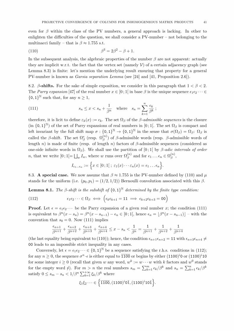
PROJECTIVE CONVERGENCE OF COLUMNS FOR INHOMOGENEOUS MATRIX PRODUCTS 41
even for β within the class of the PV numbers, a general approach is lacking. In other to
enlighten the difficulties of the question, we shall consider a PV-number – not belonging to the
multinacci family – that is β ≈ 1.755 s.t.
(110) β3 = 2β2 − β + 1.
In the subsequent analysis, the algebraic properties of the number β are not apparent: actually
they are implicit w.r.t. the fact that the vertex set (namely V) of a certain adjacency graph (see
Lemma 8.3) is finite: let’s mention the underlying result ensuring that property for a general
PV-number is known as Garsia separation Lemma (see [24] and [41, Proposition 2.6]).
8.2. β-shifts. For the sake of simple exposition, we consider in this paragraph that 1 < β < 2.
The Parry expansion [47] of the real number x ∈ [0 ; 1[ in base β is the unique sequence ε1ε2 · · · ∈0, 1N such that, for any n ≥ 1,
(111) sn ≤ x < sn +1
βnwhere sn =
n∑k=1
εkβk
;
therefore, it is licit to define εk(x) := εk. The set Ωβ of the β-admissible sequences is the closure
(in 0, 1N) of the set of Parry expansions of real numbers in [0 ; 1[. The set Ωβ is compact and
left invariant by the full shift map σ : 0, 1N → 0, 1N in the sense that σ(Ωβ) = Ωβ: Ωβ is
called the β-shift. The set Ω∗β (resp. Ω(n)β ) of β-admissible words (resp. β-admissible words of
length n) is made of finite (resp. of length n) factors of β-admissible sequences (considered as
one-side infinite words in Ωβ). We shall use the partition of [0 ; 1[ by β-adic intervals of order
n, that we write [0 ; 1[=⊔w Iw, where w runs over Ω
(n)β and for ε1 . . . εn ∈ Ω
(n)β ,
Iε1...εn :=x ∈ [0 ; 1[ ; ε1(x) · · · εn(x) = ε1 . . . εn
.
8.3. A special case. We now assume that β ≈ 1.755 is the PV-number defined by (110) and µ
stands for the uniform (i.e. (p0, p1) = (1/2, 1/2)) Bernoulli convolution associated with this β.
Lemma 8.1. The β-shift is the subshift of 0, 1N determined by the finite type condition:
(112) ε1ε2 · · · ∈ Ωβ ⇐⇒(εkεk+1 = 11 =⇒ εk+2εk+3 = 00
)Proof. Let ε = ε1ε2 · · · be the Parry expansion of a given real number x; the condition (111)
is equivalent to βn(x− sn) = βn(x− sn−1)− εn ∈ [0 ; 1[, hence εn = bβn(x− sn−1)c – with the
convention that s0 = 0. Now (111) implies
εn+1
βn+1+εn+2
βn+2+εn+3
βn+3+εn+4
βn+4≤ x− sn <
1
βn=
1
βn+1+
1
βn+2+
1
βn+4
(the last equality being equivalent to (110)); hence, the condition εn+1εn+2 = 11 with εn+3εn+4 6=00 leads to an impossible strict inequality in any cases.
Conversely, let ε = ε1ε2 · · · ∈ 0, 1N be a sequence satisfying the r.h.s. conditions in (112);
for any n ≥ 0, the sequence σn ·ε is either equal to 1100 or begins by either (1100)i0 or (1100)i10
for some integer i ≥ 0 (recall that given w any word, wk := w · · ·w with k factors and w0 stands
for the empty word /). For m > n the real numbers sm =∑m
k=1 εk/βk and sn =
∑nk=1 εk/β
k
satisfy 0 ≤ sm − sn < 1/βn∑+∞
k=1 ξk/βk where
ξ1ξ2 · · · ∈1100, (1100)i01, (1100)i101
.
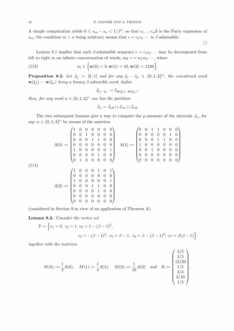
42 E. OLIVIER AND A. THOMAS
A simple computation yields 0 ≤ sm − sn < 1/βn, so that ε1 . . . εm0 is the Parry expansion of
sm; the condition m > n being arbitrary means that ε = ε1ε2 · · · is β-admissible.
Lemma 8.1 implies that each β-admissible sequence ε = ε1ε2 · · · may be decomposed from
left to right in an infinite concatenation of words, say ε = w1w2 · · · , where
(113) wi ∈
w(0) = 0,w(1) = 10,w(2) = 1100.
Proposition 8.2. Let J/ := [0 ; 1[ and for any ξ1 · · · ξn ∈ 0, 1, 2n, the concatened word
w(ξ1) · · ·w(ξn) being a binary β-admisible word, define
Jξ1···ξn := Iw(ξ1)···w(ξn) ;
then, for any word w ∈ 0, 1, 2∗ one has the partition
Jw = Jw0 t Jw1 t Jw2.
The two subsequent lemmas give a way to compute the µ-measure of the intervals Jw, for
any w ∈ 0, 1, 2∗ by means of the matrices
(114)
A(0) :=
1 0 0 0 0 0 00 0 1 0 0 0 00 0 0 1 1 0 00 0 0 0 0 0 01 0 0 0 0 0 10 0 0 0 1 0 00 1 0 0 0 0 0
A(1) :=
0 0 1 1 0 0 00 0 0 0 0 1 00 0 0 1 1 0 01 0 0 0 0 0 00 0 1 0 0 0 00 0 0 0 0 0 00 0 0 0 0 0 0
A(2) :=
1 0 0 0 1 0 10 0 0 0 0 0 01 0 0 0 0 0 10 0 0 1 1 0 00 0 0 0 1 0 00 0 0 0 0 0 00 0 0 0 0 0 0
(considered in Section 9 in view of an application of Theorem A).
Lemma 8.3. Consider the vertex set
V =v1 = 0, v2 = 1, v3 = 1− (β − 1)2,
v4 = −(β − 1)2, v5 = β − 1, v6 = β − (β − 1)2, v7 = β(β − 1)
together with the matrices
M(0) :=1
2A(0), M(1) :=
1
4A(1), M(2) :=
1
16A(2) and R :=
3/52/5
13/201/53/53/101/5
.

PROJECTIVE CONVERGENCE OF COLUMNS FOR INHOMOGENEOUS MATRIX PRODUCTS 43
Then, for any n ≥ 1 and any word ξ1 · · · ξn ∈ 0, 1, 2n
(115)
µ(
1β
(v1 + Jξ1···ξn
))...
µ(
1β
(v7 + Jξ1···ξn
)) = M(ξ1 · · · ξn)R.
Proof. For any real number γ we evaluate
µ
(1
β
(γ + Jξ1···ξn
))in the three cases when ξ1 is either 0, 1 or 2. First, consider that ξ1 = 0, so that
(β − 1)+∞∑k=1
ωkβk∈ 1
β
(γ + Jξ1···ξn
)⇐⇒ (β − 1)
+∞∑k=1
ωk+1
βk∈ 1
β
(γ′ + Jξ1···ξn
)with γ′ = γβ − ω1β(β − 1) and since ω1 ∈ 0, 1,
(116) µ
(1
β
(γ + Jξ1···ξn
))=
1
2
∑γ′∈V0(γ)
µ
(1
β
(γ′ + Jξ1···ξn
)),
where
V0(γ) :=γβ − uβ(β − 1) ; u ∈ 0, 1
.
We proceed in the same way for ξ1 = 1:
(117) µ
(1
β
(γ + Jξ1···ξn
))=
1
4
∑γ′∈V1(γ)
µ
(1
β
(γ′ + Jξ1···ξn
)),
where
V1(γ) :=γβ2 + β − (uβ + v)β(β − 1) ; u, v ∈ 0, 1
.
Finally, in the case of ξ1 = 2, one gets
(118) µ
(1
β
(γ + Jξ1···ξn
))=
1
16
∑γ′∈V2(γ)
µ
(1
β
(γ′ + Jξ1···ξn
)),
where
V2(γ) =γβ4 + β3 + β2 − (uβ3 + vβ2 + wβ + x)β(β − 1) ; u, v, w, x ∈ 0, 1
.
However, the measure µ being supported by the unit interval [0 ; 1], one has:
Lemma 8.4. γ 6∈]− 1 ;β[ =⇒ µ
(1
β
(γ + [0 ; 1[
))= 0.
Because of Lemma 8.4, we define for each e ∈ 0, 1, 2 the relation
γe−→ γ′ ⇐⇒ γ′ ∈ Ve(γ)∩]− 1 ;β[
and by definition, V is the subset of ] − 1 ;β[ containing 0 and the γ ∈] − 1 ;β[ for which there
exists a sequence e0, . . . , en in 0, 1, 2 and 0 = γ0, · · · , γn = γ in ]− 1 ;β[ (with n ≥ 0) s.t.
γ0e0−→ γ1, . . . , γn−1
en−→ γn ;

44 E. OLIVIER AND A. THOMAS
then, a direct computation gives
V =v1 = 0, v2 = 1, v3 = 1− (β − 1)2,
v4 = −(β − 1)2, v5 = β − 1, v6 = β − (β − 1)2, v7 = β(β − 1).
For e ∈ 0, 1, 2, we define A′(e) to be the 7 × 7 incident matrix s.t. for any 1 ≤ i, j ≤ 7,
the (i, j) entry of A′(e) is 1 if and only if vie−→ vj (the corresponding incidence relations are
represented by the adjacency graph in Figure 8).
0,1
0,2
20,1
22
1
1
2
2
0
0
1
00
2
0
2
1
1
Figure 8. Adjacency graph corresponding to the relation vie−→ vj (e = 0, 1, 2) between the
elements in V = v1, . . . , v7, which are the 7 vertices of the graph.
The key point is that
A′(0) = A(0), A′(1) = A(1), A′(2) = A(2)
and one deduces from (116), (117) and (118) that for any ξ ∈ 0, 1, 2N and any n ≥ 1µ(
1β
(v1 + Jξ1···ξn
))...
µ(
1β
(v7 + Jξ1···ξn
)) = M(ξ1 · · · ξn)R, where R =
µ(
1β
(v1 + [0 ; 1[
))...
µ(
1β
(v7 + [0 ; 1[
)) .
In order to compute R we consider the case n = 1 and we sum for ξ1 ∈ 0, 1, 2. Since
(Proposition 8.2) the sets Jξ1 form a partition of [0 ; 1[, we obtain that R is an eigenvector of
M(0) +M(1) +M(2). Moreover, because the sum of the two first entries in R is
µ(
0 + 1/β[0 ; 1[)
+ µ(
1/β + 1/β[0 ; 1[)
= µ(
1/β[0 ; 2[)
= µ([0 ; 1]) = 1,
the computation of this eigenvector gives the expected value for R.

PROJECTIVE CONVERGENCE OF COLUMNS FOR INHOMOGENEOUS MATRIX PRODUCTS 45
A direct consequence is the exact value of the µ-measure of the intervals Jw.
Lemma 8.5. For any ξ ∈ 0, 1, 2N and any n ≥ 1,
(119) µ (Jξ1···ξn) =
U?1M(ξ2 · · · ξn)R if ξ1 = 0
U?2M(0)M(ξ2 · · · ξn)R if ξ1 = 1
U?2M(1)M(0)M(ξ2 · · · ξn)R if ξ1 = 2.
It remains to prove that µ is a weak-Gibbs measure.
Theorem 8.6. µ is weak-Gibbs in the sense that there exists a continuous Ψ : 0, 1, 2N → Rand a sub-exponential sequence of positive constants K1,K2, . . . s.t for any ξ ∈ 0, 1, 2N,
(120)1
Kn≤
µ (Jξ1···ξn)
exp(∑n−1
k=0 Ψ(σk · ξ)) ≤ Kn.
We shall need the following theorem whose proof (see Section 9) depends on Theorem A.
Theorem 8.7. Let A(0), A(1), A(2) be the 7× 7 matrices in (114): if the vector V has positive
entries then, the sequence of the probability vectors
Πn(ω, V ) =A(ω1) · · ·A(ωn)V
‖A(ω1) · · ·A(ωn)V ‖,
converges to a probability vector V(ω), uniformly over ω ∈ 0, 1, 2N, as n→ +∞; moreover,
∆(V(ω)) ≥ U1 + U3 + U5,
except for ω ∈ 0 = 00 · · · , 2 = 22 · · · for which
V(0) = 1/5(U2 + U3 + U5 + U6 + U7) and V(2) = 1/3(U1 + U3 + U4).
Proof of Theorem 8.6. In view of Proposition 6.1, we stress that the uniform convergence
of the n-step potential of µ does not hold: to overcome this difficulty we shall introduce an
intermediate measure. Let U = U1 + · · ·+ U7; by Kolmogorov Extension Theorem, there exists
a unique measure ν on [0 ; 1] such that, for any ξ1, . . . , ξn ∈ W0,
(121) ν (Jξ1···ξn) = ‖M(ξ1 · · · ξn)R‖ = U?M(ξ1 · · · ξn)R.
Recall that for any ξ ∈ 0, 1, 2N and any n ≥ 1
Πn(ξ,R) =M(ξ1 · · · ξn)R
‖M(ξ1 · · · ξn)R‖=
A(ξ1 · · · ξn)R
‖A(ξ1 · · · ξn)R‖,
so that the n-step potential of the measure ν, that is φn : 0, 1, 2N → R s.t.
φn(ξ) = log
(U?M(ξ1)Πn−1(σ · ξ,R)
U?Πn−1(σ · ξ,R)
),
converges uniformly on 0, 1, 2N toward a continuous Ψ : 0, 1, 2N → R: indeed, by Theo-
rem 8.7 the functions ξ 7→ Πn(ξ,R) form a sequence which converges uniformly for ξ ∈ 0, 1, 2N
toward V(ξ) ∈ S7 s.t. M(a)V(ξ) 6= 0, for any ξ ∈ 0, 1, 2N and a ∈ 0, 1, 2. Therefore (Propo-
sition 6.2), the measure ν is weak Gibbs w.r.t. Ψ in the sense that there exists a sub-exponential
sequence of positive constants K1,K2, . . . s.t for any ξ ∈ 0, 1, 2N,
1
Kn≤
ν (Jξ1···ξn)
exp(∑n−1
k=0 Ψ(σk · ξ)) ≤ Kn.

46 E. OLIVIER AND A. THOMAS
Hence, the weak Gibbs property of µ (w.r.t. to Ψ) will be established if one is able to show that
(122) limn→+∞
(ν (Jξ1···ξn)
µ (Jξ1···ξn)
)1/n
= 1
uniformly for ξ = ξ1ξ2 · · · ∈ 0, 1, 2N. First, from Lemma 8.5 together with the inequalities
U?M(0) ≥ U?1 , U?M(1) ≥ U?2M(0), U?M(2) ≥ U?2M(1)M(0),
one deduces that for any ξ ∈ 0, 1, 2N and any n ≥ 1,
(123) 1 ≤ν(Jξ1···ξn)
µ(Jξ1···ξn).
Concerning the upper bound we consider the different cases for ξ1 either equal to 0, 1 or 2.
• Suppose that ξ1 ∈ [1]. From (121) and (119) and the fact that U?2M(0) = 1/2 · U?3 one
has:ν (Jξ1···ξn)
µ (Jξ1···ξn)=U?M(1)Πn−1(σ · ξ,R)
U?2M(0)Πn−1(σ · ξ,R)≤ 2 · ‖M(1)‖U?3 Πn−1(σ · ξ,R)
=2 · ‖M(1)‖Fn−1(σ · ξ)
where Fk : 0, 1, 2N → R is the continuous function s.t. Fk(ζ) = U?3 Πk(ζ,R) (and the con-
vention Π0(·, R) = R/‖R‖). By Theorem 8.7, Πk(ζ,R) tends uniformly (as k → +∞) to a
probability vector V(ζ) for any ζ ∈ 0, 1, 2N: hence, the Fk are continuous positive functions
converging uniformly (on 0, 1, 2N) toward F : 0, 1, 2N → R s.t. F (ζ) = U?3 V(ζ); however,
(Theorem 8.7 again) ∆(V(ζ)) ≥ U3 ensuring the continuous function F to be also positive: in
particular the infimum infF∗ of the Fk(ζ) for ζ ∈ 0, 1, 2N and k ≥ 0 is positive. Finally one
deduces
(124) ξ ∈ [1] =⇒ν (Jξ1···ξn)
µ (Jξ1···ξn)≤ 2 · ‖M(1)‖
infF∗.
• Suppose that ξ ∈ [0]; the functions Gk : [1] ∪ [2] → R such that Gk(ζ) = U?1 Πk(ζ,R) are
continuous, positive and converge uniformly (on [1] ∪ [2]) toward G : [1] ∪ [2] → R s.t. G(ζ) =
U?1 V(ζ): by Theorem 8.7, G is continuous and positive: in particular the infimum infG∗ of the
Gk(ζ) for ζ ∈ [1] ∪ [2] and k ≥ 0 is positive. Because ξ1 = 0, we consider the largest 1 ≤ m ≤ nfor which 0m is a prefix of ξ1 . . . ξn so that ξ1 . . . ξk = 0mξm+1 . . . ξn where ξm+1 6= 0 if m < n.
From (121) and (119) and the facts that
U?1M(0)m−1 =1
2m−1· U?1 and U?M(0)m ≤ 2m
2m· U? ≤ n
2m−1· U?
one deduces
ν (Jξ1···ξn)
µ (Jξ1···ξn)=
U?M(0)mΠn−m(σm · ξ,R)
U?1M(0)m−1Πn−m(σm · ξ,R)≤ n · U?Πn−m(σm · ξ,R)
U?1 Πn−m(σm · ξ,R).
Because ‖Πn−m(σm · ξ,R)‖ = 1 and the definition of both Gn−m and infG∗
(125) ξ ∈ [0] =⇒ν (Jξ1···ξn)
µ (Jξ1···ξn)≤
n · U?RU?1R
if m = n
n · U?Πn−m(σm · ξ,R)
Gn−m(σm · ξ)≤ n
infG∗if m < n
• Suppose that ξ ∈ [2]; the functions Hk : [1] ∪ [0] → R such that Hk(ξ) = U?5 Πk(ξ,R)
are continuous, positive and converge uniformly (on [1] ∪ [0]) toward H : [1] ∪ [0] → R s.t.
H(ξ) = U?5 V(ξ): by Theorem 8.7, H is continuous and positive and the infimum infH∗ of the

PROJECTIVE CONVERGENCE OF COLUMNS FOR INHOMOGENEOUS MATRIX PRODUCTS 47
Hk(ξ) for ξ ∈ [1] ∪ [0] and k ≥ 0 is positive. Because ξ1 = 2, we consider the largest 1 ≤ m ≤ nfor which 2m is a prefix of ξ1 . . . ξn, so that ξ1 · · · ξn = 2mξm+1 . . . ξn where ξm+1 6= 2 if m < n.
From (121) and (119) together with
U?M(2)m ≤ 3m
24m· U? ≤ 3n
24m· U? and U?2M(1)M(0)M(2)m−1 =
1
24m−1· U?5 ,
one deduces
ν (Jξ1···ξn)
µ (Jξ1···ξn)=
U?M(2)mΠn−m(σm · ξ,R)
U?2M(1)M(0)M(2)m−1Πn−m(σm · ξ,R)≤ 3n
2· U
?Πn−m(σm · ξ,R)
U?5 Πn−m(σm · ξ,R),
that is, with ‖Πn−m(σm · ξ,R)‖ = 1 and the definition of both Hn−m and infH∗
(126) ξ ∈ [2] =⇒ν (Jξ1···ξn)
µ (Jξ1···ξn)≤
3n · U?R2 · U?5R
if m = n
3n · U?Πn−m(σm · ξ,R)
2 ·Hn−m(σm · ξ)≤ 3n
2 · infH∗if m < n
It follows from (123)-(124)-(125)-(126) that (122) holds, proving the theorem.
9. An advanced application of Theorem A: proof of Theorem 8.7
This section is devoted to the full proof of Theorem 8.7 stated and used in the previous
section. The main problem is concerned with the application of Theorem A w.r.t. the matrix
products of the three 7×7 matrices, A(0), A(1), A(2) given in (114). In view of Theorem A, the
major ingredient we shall need is the following proposition.
Proposition 9.1. The sequences ω ∈ 0, 1, 2N which are (C)-regular – in the sense that A(ω) =
(A(ω1), A(ω2), . . . ) satisfies condition (C) – form the dense set
(127) X :=
(0, 1, 2N \
+∞⋃n=0
σ−n0
)∩
(0, 1, 2N \
+∞⋃n=0
σ−n2
).
The proof of Proposition 9.1 depends on the introduction of a language W ⊂ 0, 1, 2∗.
9.1. The language W. The initial idea is to find (if possible) a language W ⊂ 0, 1, 2∗
(i.e. each W ∈ W is a word with digits in 0, 1, 2 and whose length |W | is finite) with two
properties as follows. First (see Lemma 9.3 for the exact statement), W generates the sequences
in X (i.e. the ω ∈ 0, 1, 2N for which σk · ω never belong to 0, 2) in the sense that such
a ω may be written as a concatenation of words, that is ω = W0W1W2 . . . , where W1W2 . . .
are in W and W0 is a (possibly empty) strict suffix of a word in W. The second condition
is the existence of 0 ≤ λ0 < 1 ≤ Λ0 < +∞ such that A(W ) ∈ H2(Λ0) for any W ∈ W(Lemma 9.2), and A(W ) ∈ H1∩H3(λ0) when W is a concatenation of a (fixed) number of words
in W (Lemma 9.4). To construct W, notice that for s either equal to 0 or 2, the condition
that A(sk) = A(s)k ∈ H2(Λ) for any k implies Λ = +∞ (this is the reason why 0 and 2 are
(C)-singular); taking this remark into account, we begin to fix 1 ∈ W, the other words W ∈ Wbeing of the form W ′sk, for some words W ′ 6= / specified later, while s = 0 or 2, and for any
k ≥ 1: more precisely, the (non empty) prefixes W ′ of the words W ∈ W will be determined in
order to ensure that any finite word not ending by 1 has a suffix of the form W ′sk, or W ′′sk

48 E. OLIVIER AND A. THOMAS
with W ′′ suffix of W ′, while A(W ) = A(W ′sk) belongs to H2(Λ0), for a Λ0 < +∞ independent
of W (the determination of λ0 being obtained in a second step).
1
110k010k 210k
20k
002k 202k
12k
00102k 10102k 20102k
2102k1102k
10k
0k 2k
02k
102k
0102k
Figure 9. Lexicographical construction (from right to left) of the words in W (here k ≥ 1).
For instance, let’s compute successively A(2k), A(02k), A(102k), A(0102k), . . . , which gives
A(2k) =
1 0 0 0 k 0 10 0 0 0 0 0 01 0 0 0 k − 1 0 10 0 0 1 k 0 00 0 0 0 1 0 00 0 0 0 0 0 00 0 0 0 0 0 0
A(02k) =
1 0 0 0 k 0 11 0 0 0 k − 1 0 10 0 0 1 k + 1 0 00 0 0 0 0 0 01 0 0 0 k 0 10 0 0 0 1 0 00 0 0 0 0 0 0
A(102k) =
0 0 0 1 k + 1 0 00 0 0 0 1 0 01 0 0 0 k 0 11 0 0 0 k 0 10 0 0 1 k + 1 0 00 0 0 0 0 0 00 0 0 0 0 0 0
A(0102k) =
0 0 0 1 k + 1 0 01 0 0 0 k 0 11 0 0 1 2k + 1 0 10 0 0 0 0 0 00 0 0 1 k + 1 0 00 0 0 1 k + 1 0 00 0 0 0 1 0 0
A(10102k) =
1 0 0 1 2k + 1 0 10 0 0 1 k + 1 0 00 0 0 1 k + 1 0 00 0 0 1 k + 1 0 01 0 0 1 2k + 1 0 10 0 0 0 0 0 00 0 0 0 0 0 0
.

PROJECTIVE CONVERGENCE OF COLUMNS FOR INHOMOGENEOUS MATRIX PRODUCTS 49
Observe that if A(W ) ∈ H2(Λ), for any W = 2k, with k ≥ 1 (and likewise for W = 02k, 102k or
0102k) then Λ = +∞, while for W ∈⋃+∞k=110102k it is simple to check that A(W ) ∈ H2(7)
(for indeed 2 ≤ 7 · 1, 5 ≤ 7 · 1, 7k + 5 ≤ 7 · (k + 1), 7k + 5 ≤ 7 · (2k + 1) are valid inequalities,
for any k ≥ 1). Using this algorithm, leads to the language:
W :=1∪
+∞⋃k=1
010k, 110k, 210k, 20k, 002k, 00102k, 10102k, 20102k, 1102k, 2102k, 202k, 12k
,
together with the fact that A(1) ∈ H2(2), while for any k ≥ 1
A(010k) ∈ H2(8) A(110k) ∈ H2(8) A(210k) ∈ H2(6) A(20k) ∈ H2(7)A(002k) ∈ H2(12) A(00102k) ∈ H2(13) A(10102k) ∈ H2(7) A(20102k) ∈ H2(6)A(1102k) ∈ H2(8) A(2102k) ∈ H2(6) A(202k) ∈ H2(5) A(12k) ∈ H2(9)
These computations also ensure that A(W ) ∈ H3(5), for any W ∈ W.
Lemma 9.2. A(W ) ∈ H2(13) ∩H3(5), for any W ∈ W.
Lemma 9.3. Given ω = ω1ω2 · · · ∈ 0, 1, 2N one has
(i) : for any n ≥ 1, either ω1 · · ·ωn is a strict suffix W0(n) of a word in W or there exists
a possibly empty strict suffix W0(n) of a word in W and W1(n), . . . ,Wkn(n) ∈ W s.t.
ω1 · · ·ωn = W0(n)W1(n) · · ·Wkn(n) ;
(ii) : if ω ∈ X (i.e. σk · ω never belongs to 0, 2) then, there exist W1,W2, . . . in W and
W0 a possibly empty strict suffix of a word in W, s.t.
ω1ω2 · · · = W0W1W2 · · ·
Proof. (i) : Let n ≥ 1 : by definition of W, either ω1 . . . ωn is a strict suffix of a word of
W or ω1 . . . ωn has a suffix W ′ ∈ W. In the later case, there exists a word W such that
ω1 . . . ωn = WW ′. If W is neither empty nor a strict suffix of a word in W, we repeat the
procedure with W and so on and so forth with a finite induction.
(ii) : We use the decomposition in part (i) for any n ≥ 1: for the word W0(n) is a strict
suffix of a word of W, there exists k ≥ 1 such that W0(n) ∈ /, 10k, 0k, 0102k, 102k, 02k, 2k.Since ω ∈ X, the set W0(n) ; n ≥ 1 is necessarily finite. Hence, there exists a word W0
and an infinite set E0 ⊂ 1, 2, . . . such that W0(n) = W0, for any n in E0. The words
W0,W1, . . . are defined by induction: given k ≥ 0, let W0, . . . ,Wk be k+1 words for which
W0(n) = W0, . . . ,Wk(n) = Wk for any n in an infinite set Ek ⊂ 1, 2, . . . . Since ω ∈ X, there
cannot exist infinitely many words W ∈ W such that W0 . . .WkW is a prefix of ω1 . . . ωn for a
n ≥ 1. Hence, there exists Wk+1 s.t. W0(n) = W0, . . . ,Wk+1(n) = Wk+1 for any n in an infinite
set Ek+1 ⊂ Ek: the induction holds, so that ω1ω2 · · · = W0W1W2 · · · .
The language W has two important drawbacks w.r.t. condition (C). First, for many W
in W the matrices A(W ) belongs to H1, but (unfortunately) there are words in W for which
this is not true: for instance, A(010) =
0 0 0 1 1 0 01 0 0 0 0 0 11 0 0 1 1 0 00 0 0 0 0 0 00 0 0 1 1 0 00 0 0 1 1 0 00 0 0 1 1 0 0
(we shall see (Lemma 9.5) that

50 E. OLIVIER AND A. THOMAS
A(W ) ∈ H1 as soon as W is factorized by a concatenation of at least 13 words in W). Secondly,
the constant λ = 5 in Lemma 9.2 is larger than 1. The following lemma is crucial (its proof is
given in § 9.2 below).
Lemma 9.4. If W ∈ 0, 1, 2∗ is factorized by a concatenation of 130 (= 10 · 13) words in
W, then:
A(W ) ∈ H1 ∩H3 (3/4) .
Proof of Proposition 9.1. The fact that 0 and 2 are (C)-singular may be checked directly.
To prove that an arbitrary given ω ∈ X is necessarily (C)-regular we begin with Lemma 9.3 to
write ω = W0W1W2 · · · , where W0 is a possibly empty strict suffix of a word in W and each
W1,W2, . . . are words in W. Let 0 = s0 = s1 and for k ≥ 1 define:
sk+1 =∑130k
i=0|Wi|.
This leads to the recoding ω = Ws2Ws3 · · · , where Ws2 = W0W1 · · ·W130 = ω1 · · ·ωs2 , while for
k ≥ 2,
Wsk+1= W130(k−1)+1 · · ·W130k = ωsk+1 · · ·ωsk+1
.
The latter notations are consistent with setting W0 = / and for n ≥ 1, k ≥ 0 and sk+1 ≤ n < sk+2
Wn = ωsk+1 · · ·ωn = Wsk+1W ′n where W ′n := ωsk+1+1 · · ·ωn ;
in other words, ω1 · · ·ωn = Wn when n < s3, while for n ≥ s3,
ω1 · · ·ωn = Ws2 · · · WskWn = Ws2 · · · WskWsk+1W ′n.
(For sk+1 ≤ n < sk+2, the word W ′n a strict prefix of Wsk+2.)
130 130130
Figure 10. Each ω ∈ X may be recoded by writing ω1ω2 · · · = Ws2Ws3 · · · , where each word
Wsk is factorized by a concatenation of 130 words inW; the sequence 0 = s0 = s1 < s2 < · · · for
condition (C) is defined in consequence, that is sk = |W2 · · · Wsk | and for each sk+1 ≤ n < sk+2
(with k ≥ 0) Wn = ωsk+1 · · ·ωn = Wsk+1W′n is also factorized by a concatenation of 130 words
in W; the importance of the number 130 comes from crucial Lemma 9.4.
With the notations of Definition 1.1, one has Pn = A(ω1 · · ·ωn) = PskQn, where we stress
on the key correspondence
(128) Qn = A(Wn).

PROJECTIVE CONVERGENCE OF COLUMNS FOR INHOMOGENEOUS MATRIX PRODUCTS 51
The first and the third parts of condition (C) are satisfied since by definition of Wn and of the
sequence (s0, s1, . . . ), Lemma 9.4 ensures that
(129) n ≥ s2 =⇒ Qn = A(Wn) ∈ H1 ∩H3 (3/4)
It remains to establish the existence of a constant Λ ≥ 1 (depending on ω) s.t.
(130) n ≥ s2 =⇒ Qn = A(Wn) ∈ H2(Λ).
Suppose s2 ≤ sk+1 ≤ n < sk+2; by construction, Wn = Wsk+1W ′n, where W ′n is a (possibly
empty) strict prefix of Wsk+2: actually, either W ′n = W ′n or W ′n = W130k+1 · · ·W130k+mW
′n,
where 1 ≤ m < 130, while W ′n is a strict prefix of a word in W. However (Lemma 9.2) we know
that A(Wi) ∈ H2(13) ∩H3(5), for any i > 0 and by part (ii) of Lemma 2.9),
A(Wn) ∈ H2
( (1 + 5 + · · ·+ 52·130−2
)· 13 + 52·130−1 · ΛA(W ′n)
);
therefore A(Wn) ∈ H2
(5260(4 + Λ′)
), where Λ′ stands for the maximum of the ΛA(W ′) over W ′
being any prefix of a word in W. The inequality Λ′ < +∞ is valid, because either W ′ ∈ W and
A(W ′) ∈ H2(13) or W ′ 6∈ W which is only possible for
W ′ ∈ /, 0, 00, 001, 0010, 01, 11, 10, 101, 1010, 2, 201, 2010, 21.
9.2. Proof of Lemma 9.4. For Proposition 9.1 to be completely established, it remains to
prove Lemma 9.4. The argument – given in § 9.2.4 – depends on a key lemma (Lemma 9.5)
established in § 9.2.1 together with several properties of two adjacency graphs – (Γ1) and (Γ2) –
that we consider in § 9.2.2 and § 9.2.3 respectively.
9.2.1. Key Lemma. The following lemma shows – in part (iii) – that A(W ) ∈ H1 as soon as W
is factorized by a concatenation of at least 13 words inW. Parts (i) and (ii) will be determinant
in the final argument proving Lemma 9.4 in § 9.2.4, and use the following set of four column
vectors (that we represent by convenience by four 7-uplets):
(131) T2 :=
(1, 0, 1, 1, 1, 0, 0), (1, 1, 1, 0, 1, 1, 0), (1, 1, 1, 0, 1, 1, 1), (1, 1, 1, 1, 1, 0, 0).
Lemma 9.5. If W ∈ 0, 1, 2∗ is factorized by a concatenation of 13 words in W, then
(i) :
∆(A(W )U1),∆(A(W )U3),∆(A(W )U5)∩ T2 6= ∅;
(ii) : #Col(A(W )) ≤ 2 ;
(iii) : A(W ) ∈ H1.
Proof. We shall begin to verify that any W = W1 · · ·W13 with Wi ∈ W has a factor W ′ s.t.
A(W ′) satisfies (i–ii–iii). First, suppose that 01 is a factor of W2 . . .W10 and write W2 . . .W10 =
X01Y . On the one hand, it is necessary that W1X 6= 0 and thus, W1X has suffix in L′ :=
00, 10, 20, 1, 2; on the other hand, it is also necessary that YW11W12W13 has prefix in
L′′ := 00, 01, 02, 10, 110, 111, 112, 12, 20, 21, 22.
Hence (see Figure 11 – left) W is factorized by a word belonging to L′01L′′ and (see § 11.1 in
Appendix 11) each word in L′01L′′ satisfies (i–ii–iii). For the second case, suppose that 21 is
a factor of W2 . . .W10 that is, W2 . . .W10 = X21Y ; the word YW11W12W13 has necessarily a
prefix in
L′′′ := 0, 10, 110, 111, 112, 12, 20, 21, 22 ;

52 E. OLIVIER AND A. THOMAS
like in the first case (see Figure 11 – right) W is factorized by a word W ′ ∈ L′21L′′′ and (see
§ 11.2 in Appendix 11) each word in L′21L′′′ satisfies (i–ii–iii).
01
00102012
00010210110111112122021
22
21
00102012
01011011111212202122
Figure 11. How to obtain the words in L′01L′′ (left) and in L′21L′′′ (right).
Finally, it remains to consider the case where neither 01 nor 21 is a factor of W2 . . .W10: in
particular, this means that W2 · · ·W10 = 1kW ′ with k ≥ 0 and W ′ ∈ 0, 2∗ (it is here where the
13 words in W will prove to be needed). Notice that A(1), . . . , A(1111) do not satisfy (i–ii–iii),
while
A(11111) =
3 0 3 2 1 0 00 0 0 0 0 0 01 0 3 3 1 0 01 0 1 3 2 0 02 0 1 1 1 0 00 0 0 0 0 0 00 0 0 0 0 0 0
does satisfy this property: hence, W has a factor W ′ (= 11111) with A(W ′) satisfying (i–ii–iii),
as soon as k ≥ 5. Now, suppose that k ≤ 4, so that W6 · · ·W10 ∈ 0, 2∗ (indeed the worst case
arises for k = 4 with W2W3W4W5 = 1111). The definition of W implies that each word W6,
W7, W8, W9, W10 must be either 20k, 002k or 202k (for some k ≥ 1). Then, it is necessary that
02 is a factor of both W6W7 and W8W9: this implies that W6 · · ·W10 has a factor of the form
0x2y0z2t0u with x, y, z, t, u ≥ 1. On the one hand, if t = 1 then z = 1, 2, 3, . . . and 0x2y0z2t0u
is factorized by either 2020, 20020 or 00020; on the other hand, if t ≥ 2, the word 0x2y0z2t0u is
factorized by 220. One concludes this case, since W is factorized by a word W ′ which is either
equal to 2020, 20020, 00020 or 220 and which (see § 11.3 in Appendix 11) satisfies (i–ii–iii).
We now conclude with the general case of W ∈ 0, 1, 2∗ which is factorized by W1 · · ·W13
with Wi ∈ W. Let W ′ be the factor of W1 · · ·W13 s.t. A(W ′) satisfies (i–ii–iii) and notice
that A(W ′) ∈ H1. Because A(W ′) satisfies (i), a direct verification shows that both A(W ′i)
and A(iW ′) satisfy (i) for any i = 0, 1, 2: hence, by a finite induction, A(W ) also satisfies
(i). The fact that (ii–iii) holds for A(W ) follows from Lemma 2.10: because A(W ′) ∈ H1 and
#Col(A(W ′)) ≤ 2, part (e) of Lemma 2.10 ensures that #Col(A(W )) ≤ 2 and part (f) that
A(W ) ∈ H1.

PROJECTIVE CONVERGENCE OF COLUMNS FOR INHOMOGENEOUS MATRIX PRODUCTS 53
9.2.2. The adjacency graph (Γ1). We begin to define the infinite adjacency graph (Γ0) whose
vertex set Vert(Γ0) is made of the nonzero 7× 1 vectors (represented for convenience by) the 7-
uplets (x1, . . . , x7) having nonnegative integral entries and obtained from one of the basis vector
U1, . . . , U7 by successive left multiplication with the matrices A(0), A(1) and A(2). For instance,
(0, 0, 1, 1, 0, 0, 0)ωn−→· · · ω1−→(x, 0, y, z, t, 0, 0)
is a path in (Γ0) so that A(ω1 · · ·ωn)(0, 0, 1, 1, 0, 0, 0) = (x, 0, y, z, t, 0, 0). Setting V ∼ V ′
whenever ∆(V ) = ∆(V ′) gives an equivalent relation on Vert(Γ0): the quotient space Vert(Γ0)/∼is made of finitely many classes of equivalence, each ones being uniquely represented by a 7-uplet
(a1, . . . , a7) ∈ ∗, 0, 1, 2, . . . 7: here (a1, . . . , a7) represents the set VkNk=1 (1 ≤ N ≤ +∞) of
all the nonzero 7× 1 vectors in a given class of equivalence, with ai either equal to supkU?i Vkor ∗ if either supkU?i Vk is finite or infinite respectfully. This leads to introduce the adjacency
graph (Γ1) whose vertex set is Vert(Γ1) = Vert(Γ0)/∼ an whose paths are obtained by quotient
projection from the paths in (Γ0): the representation of (Γ1) is given in Figure 13 of Appendix 10.
The set Vert(Γ1) may be written as a partition V1 t V2, where
V2 :=
(∗, 0, ∗, ∗, ∗, 0, 0), (∗, ∗, ∗, 0, ∗, ∗, 0), (∗, ∗, ∗, 0, ∗, ∗, ∗), (∗, ∗, ∗, ∗, ∗, 0, 0)
By an abuse of notations the vertices in Vert(Γ1) may be considered as usual 7× 1 vectors, with
for instance ‖(∗, 0, ∗, ∗, ∗, 0, 0)‖ = +∞ and ∆(∗, 0, ∗, ∗, ∗, 0, 0) = (1, 0, 1, 1, 1, 0, 0); but we may
also note (x1, . . . , x7) ∈ (y1, . . . , y7), when (y1, . . . , y7) is considered as a class of equivalence.
The set of column vectors T2 considered in Lemma 9.5 is ∆(V2).
Lemma 9.6 (Synchronization lemma). The following proposition holds
(a) : for any W ∈ 0, 1, 2∗ and any 1 ≤ i ≤ 7
A(W )Uj 6= 0 =⇒ ∃V ∈ T2, ∆(A(W )Uj) ≤ V ;
(b) : if V ∈ V1 then A(i)V ≤ (2, 2, 2, 2, 2, 2, 2), for any i = 0, 1, 2;
(c) : if V ∈ V2 then A(i)V ∈ V2, for any i = 0, 1, 2;
(d) : in the subgraph (Γ′1) of (Γ1) with vertices in V2 (see Figure 12), the words W ∈ 0, 1, 2∗
of length |W | ≥ 3 are synchronizing: in other words, if V and V ′ are two d × 1 vectors with
nonnegative entries s.t. both ∆(V ) and ∆(V ′) belong to T2, then
|W | ≥ 3 =⇒ ∆(A(W )V ) = ∆(A(W )V ′) ;
(e) : let V be a vector having positive entries; then, for any word W ∈ 0, 1, 2∗,
W 6= / =⇒ ∆(A(W )V ) ∈ T2 ;
(f) : let V be a vector having positive entries; then, for any word W,W ′ ∈ 0, 1, 2∗,
|W | ≥ 3 =⇒ ∆(A(W )V ) = ∆(A(WW ′)V ).
Proof. Parts (a), (b) and (c) are verified directly on (Γ1) while (d) is clear from the subgraph
(Γ′1) (see Figure 12): the words in 00, 01, 11, 2 being synchronizing, each word W ∈ 0, 1, 2∗
with |W | ≥ 3 is synchronizing as well, i.e. if W = ω1 · · ·ωn ∈ 0, 1, 2n for n ≥ 3 and if
V1ω1−→· · · ωn−→V2 and V ′1
ω1−→· · · ωn−→V ′2
are two paths in (Γ′1) then it is necessary that V2 = V ′2 . For parts (e) and (f), take a vector V
with positive entries: then by direct verification one gets ∆(A(i)V ) ∈ T2, for i = 1, 2, 3 and (e)
follows from (c); part (f) is a consequence (e) and of the synchronization property in (d).

54 E. OLIVIER AND A. THOMAS
0
1
0
21
( ,0, , , ,0,0) 1,2( , , ,0, , ,0)
( , , ,0, , , ) 0
2
0
1,2
( , , , , ,0,0)* * * * * *
******
****
***
*
Figure 12. Subgraph (Γ′1) of (Γ1) with vertices (a1, . . . , a7) ∈ V2: each word in W ∈00, 01, 11, 2 is synchronizing (in this subgraph) in the sense that each path coded byW ends on the same vertex: it follows that a word W ′ ∈ 0, 1, 2∗ with |W ′| ≥ 3 issynchronizing as well.
9.2.3. The adjacency graph (Γ2). The final argument leading to Lemma 9.4 stands on a
doubling property (Lemma 9.7) displayed by a second adjacency graph (Γ2), related to the graph
(Γ1) introduced in § 9.2.2, but defined in a slightly different way. Each V ∈ Vert(Γ2) is a d× 1
nonzero vector with nonnegative integral entries and represents the set of d× 1 vectors V ′ 6= 0
with nonnegative integral entries such that ∆(V ′) = ∆(V ) and V ′ ≥ V : then, the labelled edge
Vi−→V ′ in (Γ2) means A(i)V ≥ V ′ and ∆(A(i)V ) = ∆(V ′). By definition T2 ⊂ Vert(Γ2),
all the labeled edges of (Γ2) are obtained by starting from one vertex in T2 and making all
the possible (left) multiplication by either A(0), A(1) or A(2). Among the infinitely many
possibilities of an adjacency graph satisfying the previous specifications, we have chosen one
– namely (Γ2) – with finitely many vertices with the additional property that each V ∈ Vert(Γ2)
satisfies V ≤ (2, . . . , 2). (A representation of (Γ2) is given in Figure 14 in Appendix 10). We
shall use the important fact that most of the paths of (Γ2) starting from a vertex in T2 terminate
on a vertex in 2T2, while all paths starting from a vertex in 2T2 terminate on a vertex in 2T2.
Lemma 9.7 (Doubling property). Let W = ω1 · · ·ωn ∈ 0, 1, 2n be factorized by a concatena-
tion of 3 13 words in W but not factorized by 001001; then, for any nonnegative vector V ,
∆(V ) ∈ T2 =⇒(
∆(A(W )V ) ∈ T2 and V ≥ a ·∆(V ) =⇒ A(W )V ≥ 2a ·∆(A(W )V )).
Proof. Suppose that W = ω1 · · ·ωn ∈ 0, 1, 2∗ is factorized by ωi · · ·ωj = W1 · · ·W13 with
Wi ∈ W but not factorized by 001001. Hence, the mirror word ωj · · ·ωi is a concatenation of at
least 13 words of the form 0k, 1 or 2k with k ≥ 1, without being factorized by 100100. We claim
that a path in (Γ2), labelled by ωj · · ·ωi and starting from a vertex in T2 terminates in 2T2:
indeed (see Figure 14) the longest paths (longest w.r.t. the number of blocks of the form 0k, 1
or 2k), not factorized by 100100 and whose terminal vertex does not belong to 2T2, are those
joining (1, 0, 1, 1, 1, 0, 0) to (2, 2, 2, 0, 2, 2, 1) and labelled by words of the form 00010010212k010;
these words are concatenations of the 11 words 000, 1, 00, 1, 0, 2, 1, 2k, 0, 1, 0.
3Actually 12 words are sufficient: we state the lemma with 13 instead because of the 13 words in Lemma 9.5.

PROJECTIVE CONVERGENCE OF COLUMNS FOR INHOMOGENEOUS MATRIX PRODUCTS 55
9.2.4. Proof of Lemma 9.4. Consider W := ω1 · · ·ωn = XW1 · · ·W10Y , where X,Y ∈0, 1, 2∗ and each W1, . . . ,W10 is a concatenation of 13 words in W (making W1 · · ·W10 a
concatenation of 130 words in W). The assertion A(W ) ∈ H1 is proved in Lemma 9.5. From
this lemma, #Col(A(W10Y )) ≤ 2 and there exists at least one column index j0 such that
∆(A(W10Y )Uj0
)∈ T2 and ∆
(A(W10Y )Uj
)≤ ∆
(A(W10Y )Uj0
)for any j: hence, by part (c) of
Lemma 9.6
(132) ∆(A(W10Y )Uj0
), . . . ,∆
(A(XW1 · · ·W9W10Y )Uj0
)= ∆
(A(W )Uj0
)∈ T2.
If #Col(A(W )) = 1 then A(W ) ∈ H3 (λ) for any λ ≥ 0. We now assume that #Col(A(W )) = 2
so that it is licit to consider any arbitrary column index, say j′, s.t. 0 < ∆(A(W )Uj′
)<
∆(A(W )Uj0
). One deduce from (132) and the synchronization property (part (d) of Lemma
9.6) that
(133) T2 63 ∆(A(ω4 · · ·ωn)Uj′
)< ∆
(A(ω4 · · ·ωn)Uj0
)∈ T2.
However – in view of graph (Γ1) – this is possible only if A(ω4 · · ·ωn)Uj′ ∈ Vert(Γ1) \ V2 = V1,
so that (part (b) of Lemma 9.6)
(134) A(ω4 · · ·ωn)Uj′ ≤ (2, 2, 2, 2, 2, 2, 2) and A(W )Uj′ ≤ 33 · (2, 2, 2, 2, 2, 2, 2).
We claim that the following implication holds for any j:
(135) ∆(A(W10Y )Uj
)∈ T2 =⇒ A(W )Uj ≥ 29 ·∆
(A(W )Uj
).
Take any j s.t. ∆(A(W10Y )Uj) ∈ T2 and j′ with 0 < ∆(A(W )Uj′) < ∆(A(W )Uj). It follows
from (134) and (135) that ‖A(W )Uj′‖ ≤ 7 · 33 · 2 ≤(7 · 33 · 2/29
)A(W )Uj(i), for any index
1 ≤ i ≤ 7 s.t. A(W )Uj(i) 6= 0: this means A(W ) ∈ H3
(7 · 33 · 2/29
)⊂ H3 (3/4).
To complete the proof of Lemma 9.4 it remains to establish (135), for which the graph (Γ2) is
crucial. The key point is #Col(A(W )) = 2 implies W cannot be factorized by 001001: indeed,
on the contrary – for A(001001) being a rank one matrix – the matrix A(W ) would be also of
rank one and #Col(A(W )) would be equal to 1. In particular each word W9,W8, . . . , XW1 is
not factorized by 001001 and applying Lemma 9.7 yields:
A(W10Y )Uj ≥ 1 ·∆(A(W10Y )Uj
)∈ T2
A(W9)A(W10Y )Uj = A(W9W10Y )Uj ≥ 2 ·∆(A(W9W10Y )Uj
)∈ T2
A(W8)A(W9W10Y )Uj = A(W8W9W10Y )Uj ≥ 22 ·∆(A(W8W9W10Y )Uj
)∈ T2
...
A(XW1)A(W2 · · ·W10Y )Uj = A(XW1 · · ·W10Y )Uj ≥ 29 ·∆(A(XW1 · · ·W10Y )Uj
)∈ T2.
Hence (135) is proved as well as Lemma 9.4.
9.3. Proof of Theorem 8.7. Let V ∈ S7 with positive entries. By part (e) of Lemma 9.6
the subshift ΩV – i.e. the compact shift-invariant subset of 0, 1, 2N made of the sequences
ω s.t. A(ω1 · · ·ωn)V 6= 0, for any n ≥ 1 – coincides with 0, 1, 2N. Moreover, according
to Proposition 9.1, the (C)-regular ω – in the sense that A(ω) = (A(ω1), A(ω2), . . . ) satisfies

56 E. OLIVIER AND A. THOMAS
condition (C) – form the dense subset 0, 1, 2N that is
X :=
(0, 1, 2N \
+∞⋃n=0
σ−n0
)∩
(0, 1, 2N \
+∞⋃n=0
σ−n2
).
To establish the uniform convergence of Πn(ω, V ) for ω ∈ 0, 1, 2N, we want to apply Proposi-
ton 6.5, which is the suitable form of Theorem A for the uniform convergence (Recall that we
note ωi,j = ωi+1 . . . ωj for any ω = ω1ω2 · · · ∈ 0, 1, 2N and 0 ≤ i ≤ j, in particular ωi,i = /.)• First, consider ω ∈ X. To check the conditions (U1.1) and (U1.2) in part (i) of Proposi-
ton 6.5, let n ≥ 1 and consider ξ ∈ [ω1 · · ·ωn] (i.e. ξ0,n = ω0,n). Part (ii) of Lemma 9.3
ensures that ω = ω1ω2 · · · = W0W1W2 · · · , where W0 is a possibly empty strict suffix of a
word in W, and W1,W2, . . . are words in W. Let p = p(n) ≥ 0 be the maximal rank such
that W0 · · ·Wp = ω0,ψ′(n) is a prefix of ω0,n. For n large enough, there exists an integer ψ(n),
with 0 ≤ ψ(n) ≤ ψ′(n) ≤ n and s.t.
W0 . . .Wp−3 = ω0,ψ(n) and Wp−2Wp−1Wpξψ′(n),n+r = ξψ(n),n+r,
where r ≥ 0 is arbitrarily given. Notice that n 7→ ψ(n) only depends on ω and that ψ(n)→ +∞as n→ +∞. Consider the vector
(136) Xr = A(ξψ(n),n+r)V = A(Wp−2Wp−1Wpξψ′(n),n+r)V ;
here, the key point is the synchronization property (f) in Lemma 9.6 which implies ∆(Xr) =
∆(X0), for any r ≥ 0, proving that (U1.2) holds. As for (U1.1), it remains to prove the following
lemma.
Lemma 9.8. The exists a constant Λ ≥ 1, such that, A(ξψ(n),n+r) ∈ H2(Λ), for any r ≥ 0.
Proof. According to part (i) of Lemma 9.3), it is possible to write ξψ(n),n+r = W ′0 . . .W′q where
W ′0 is a possibly empty strict suffix of a word in W, and W ′1, . . . ,W′q are words in W. For W ′0
being a strict suffix of a word of W, there exists k ≥ 1 s.t.
W ′0 ∈ /, 10k, 0k, 02k, 2k, 0102k, 102k
and since W ′0 is also a prefix of Wp−2Wp−1Wpξn,n+r, it is necessary that
W ′0 ∈ /, 10, 100, 0, 00, 2, 0102.
We note λ0 and Λ0 s.t. A(W ) ∈ H2(Λ0) ∩ H3(λ0), for any W ∈ /, 10, 100, 0, 00, 2, 0102.Moreover (Lemma 9.2) A(W ′i ) ∈ H2(13) ∩ H3(5) for any 1 ≤ i ≤ q. With q = 130 · a + b
(0 ≤ b < 130) being the euclidean division of q by 130, one writes
W ′0 · · ·W ′q = W ′0W′1 · · ·W ′bW ′1 · · · W ′a,
where each word W ′i is a concatenation of 130 words in W: part (ii) of Lemma 2.9 implies
W ′1 · · ·W ′b ∈ H2(Λ′) and W ′i ∈ H2(Λ′) for Λ′ = 13∑129
k=0 5k while Lemma 9.4 ensures W ′i ∈H3(3/4). Finally (part (ii) of Lemma 2.9 again), one concludes that A(W ′0 . . .W
′q) ∈ H2(Λ),
where
(137) Λ = Λ0 + λ0Λ′ + λ05bΛ′+∞∑k=0
(3
4
)k.

PROJECTIVE CONVERGENCE OF COLUMNS FOR INHOMOGENEOUS MATRIX PRODUCTS 57
• Consider now ω = w0, where w is a (possibly empty) word on 0, . . . , a, we shall verify
the assertions (U2) and (U3) in part (ii) of Proposition 6.5. First, (U2.1) is satisfied, for one
checks directly that
limn→+∞
∥∥∥∥ A(0n)
‖A(0n)‖− C0U
?1
∥∥∥∥ = 0, where C0 = (0, 1/5, 1/5, 0, 1/5, 1/5, 1/5),
and (U2.2) is satisfied because A(0)C0 = C0 and A(s1s2)C0 ∈ V2 for s1s2 ∈ 0, 1, 2 × 1, 2.To verify (U3.1)− (U3.2)− (U3.3), consider n large enough in order that σn−2 · ω = 0, let
ξ ∈ [ω1 · · ·ωn] and r ≥ 0. Let m be the integer s.t. ξn−2,m+2 = 0m−n+4 with n ≤ m+ 2 ≤ n+ r
and maximal w.r.t this identity (in the notations of Proposition 6.5 we take ϕ(n) = n−2): hence
condition (U3.1) – i.e. ξ ∈ [ω1 · · ·ωm] – is satisfied by definition. Then, there exists a word W ,
either empty or beginning by 1 or 2, such that ξn−2,n+r = 0m−n+4W . According to part (i) of
Lemma 9.3, we write W = W0 . . .Wp where W0 is a possibly empty strict suffix of a word in W,
and W1, . . . ,Wp are words in W. If W0 6= / we claim that W0 ∈⋃+∞k=110k, 2k, 102k; hence W ′0
defined to be either equal to 0W0 or 00W0, belongs to W. If W0 = / we put W ′0 = /, so there
exists 0 ≤ j ≤ 2 s.t. ξn−2,n+r = 0m−n+20jW ′0W1 · · ·Wp that is:
ξm,n+r = 0jW ′0W1 · · ·Wp.
Condition (U3.3) holds by the following lemma (obtained by a direct systematic verification)
Lemma 9.9. ∀w ∈ 0, 1, 2∗, U?1A(w) 6= 0.
Condition (U3.2) follows from the following lemma, that can be proved in the same way as
(137):
Lemma 9.10. There exists a constant Λ ≥ 1 s.t. for any 0 ≤ j ≤ 2, q ≥ 0, W ′′0 ∈ / ∪W and
W ′′1 , . . . ,W′′q ∈ W, one has A(0jW ′′0 · · ·W ′′q ) ∈ H2(Λ).
• The verification of the conditions (U2) and (U3) about ω = w2 is similar to the case of
ω = w0, using the fact that
limn→+∞
∥∥∥∥ A(2n)
‖A(2n)‖− C2U
?5
∥∥∥∥ = 0, where C2 = (1/3, 0, 1/3, 1/3, 0, 0, 0).
The proof of Theorem 8.7 is complete.

58 E. OLIVIER AND A. THOMAS
10. Appendix: The adjacency graphs (Γ1) and (Γ2)
(1,1,0,0,1,0,0) (0,0,1,1,0,0,0)
(0,0,0,0,0,1,0)
(1,0,1,0,0,0,0)
2
1
(0,0,1,0,0,0,0)
(0,0,0,0,1,0,0)
(0,0,0,1,0,0,0)
2
(1,0,0,0,0,0,0)
(1,0,0,0,1,0,0)
(0,1,0,0,0,0,0)
(0,0,0,0,0,0,1)
(0,1,1,0,0,1,0)
(0,0,0,0,1,0,1) (0,1,1,0,0,0,0)
(0,0,1,0,1,1,0)0
0
0
0 1
0
2
1
2
1
(0,0,1,0,0,1,0)
00
0
12
1
0
1
0
2 20
1
2
2
0
(0,1,0,0,0,0,1)
1
1
02
0
0
(1,0,0,1,1,0,0)
2
0
1
21
0
1
1,2
0
0
21
(2,0,1,0,1,0,0)(1,0,1,0,1,1,1)
( ,0, , , ,0,0)
1,2
( , , ,0, , ,0)
( , , ,0, , , )
0
(1,2,1,0,1,0,0)
2
212
0
0
1,20
(1,0,2,0,1,1,0)
0
0
2
0
(1,0,2,1,0,0,0)
1
10
0
1,2
( , , , , ,0,0)* * * * * *
******
****
***
*
1
Figure 13. A representation of (Γ1); for instance the vertex (1, 0, 2, 1, 0, 0, 0) corre-sponds to
(1, 0, 1, 1, 0, 0, 0), (1, 0, 2, 1, 0, 0, 0)
while
(∗, 0, ∗, ∗, ∗, 0, 0) =
(x, 0, y, z, t, 0, 0) ; x, y, z, t = 1, 2, . . .
;
one has the partition Vert(Γ1) = V1 t V2, where
V2 :=
(∗, 0, ∗, ∗, ∗, 0, 0), (∗, ∗, ∗, 0, ∗, ∗, 0), (∗, ∗, ∗, 0, ∗, ∗, ∗), (∗, ∗, ∗, ∗, ∗, 0, 0)
;
notice that (x1, . . . , x7) ∈ V1 = Vert(Γ1) \ V2 implies (x1, . . . , x7) ≤ (2, 2, 2, 2, 2, 2, 2).

PROJECTIVE CONVERGENCE OF COLUMNS FOR INHOMOGENEOUS MATRIX PRODUCTS 59
(2,2,2,0,2,2,1)(2,2,2,0,2,1,0)(2,1,2,0,2,2,1)
(2,1,2,2,2,0,0) (2,1,2,0,2,1,0)(2,0,2,2,1,0,0)(2,1,1,1,2,0,0) 1
1
1
1
2
2
2
0
0
0
1,2
1
0
00
2
20
2
2
0
(1,0,1,1,1,0,0) (1,1,2,0,1,1,0)
(1,1,2,1,1,0,0)(1,1,2,0,1,1,1)(1,1,1,1,1,0,0)
(1,1,1,0,2,1,1)(1,1,1,0,1,1,0) (1,1,2,0,2,2,1)
1,21,2
1
1
2
2
0
0
1
1
1
00
00
0
1,2
(1,1,1,0,1,1,1)
0
2
0
(2,0,1,1,1,0,0)
(2,2,2,0,2,2,0)
(2,0,2,2,2,0,0)(2,2,2,0,2,2,2)
(2,2,2,2,2,0,0)
1,2
1,2
0
10
02
2
1
1 0
1,2
1
Figure 14. Representation of the adjacency graph denoted by (Γ2) : the word-codesW ∈ 0, 1, 2∗ of the ”longest” paths not entering 2T2 (red vertices) and not factorizedby 100100 are of the form W = 00010010212k010 (k ≥ 1); they are represented in bluein the adjacency graph. The green triangle shows the ”forbidden” cycle 100100100 · · · .

60 E. OLIVIER AND A. THOMAS
11. Appendix: Verification for matrix products in Lemma 9.5
11.1. First case. We check that A(W ) satisfies parts (i-ii-iii) of Lemma 9.5, for any W ∈L′01L′′.• for w ∈ 000100, 01, 02, 10
A(000100) =
1 0 0 0 0 0 11 0 0 0 0 0 12 0 0 0 0 0 20 0 0 0 0 0 02 1 0 0 0 0 12 0 0 0 0 0 22 0 0 0 0 0 1
A(000101) =
1 0 1 0 0 0 01 0 1 0 0 0 01 0 2 0 0 0 00 0 0 0 0 0 01 0 2 1 0 0 01 0 2 0 0 0 01 0 2 1 0 0 0
A(000102) =
0 0 0 1 2 0 00 0 0 1 2 0 00 0 0 1 3 0 00 0 0 0 0 0 01 0 0 1 3 0 10 0 0 1 3 0 01 0 0 1 3 0 1
A(000110) =
2 0 0 0 0 0 12 0 0 0 0 0 12 0 0 0 0 0 10 0 0 0 0 0 03 0 0 1 1 0 12 0 0 0 0 0 11 0 0 1 1 0 1
• 000111 is a prefix of each word in 0001110, 111, 112 and
A(000111) =
1 0 2 1 0 0 01 0 2 1 0 0 01 0 2 1 0 0 00 0 0 0 0 0 01 0 3 3 1 0 01 0 2 1 0 0 02 0 1 1 1 0 0
• for w = 000112, one has
A(000112) =
1 0 0 1 3 0 11 0 0 1 3 0 11 0 0 1 3 0 10 0 0 0 0 0 03 0 0 1 4 0 31 0 0 1 3 0 11 0 0 2 3 0 1
• 00012 is a prefix of each word in 000120, 21, 22 and
A(00012) =
1 0 0 1 1 0 11 0 0 1 1 0 11 0 0 1 1 0 10 0 0 0 0 0 01 0 0 2 3 0 11 0 0 1 1 0 12 0 0 0 1 0 2

PROJECTIVE CONVERGENCE OF COLUMNS FOR INHOMOGENEOUS MATRIX PRODUCTS 61
• 1001 is prefix of each word in 1001L′′ and
A(1001) =
0 0 1 1 0 0 00 0 1 1 0 0 00 0 1 1 0 1 00 0 1 1 0 0 00 0 1 1 0 0 00 0 0 0 0 0 00 0 0 0 0 0 0
• each word in 2001L′′ has a prefix in 20010, 1, 2
A(20010) =
1 0 0 2 3 0 10 0 0 0 0 0 01 0 0 1 1 0 10 0 0 1 2 0 00 0 0 1 2 0 00 0 0 0 0 0 00 0 0 0 0 0 0
A(20011) =
3 0 1 2 2 0 00 0 0 0 0 0 02 0 1 1 1 0 01 0 0 1 1 0 01 0 0 1 1 0 00 0 0 0 0 0 00 0 0 0 0 0 0
A(20012) =
2 0 0 3 4 0 20 0 0 0 0 0 01 0 0 2 3 0 11 0 0 1 1 0 11 0 0 1 1 0 10 0 0 0 0 0 00 0 0 0 0 0 0
• 1010 is a prefix of each word in 10100, 01, 02 and
A(1010) =
1 0 0 1 1 0 00 0 0 1 1 0 00 0 0 1 1 0 00 0 0 1 1 0 01 0 0 1 1 0 00 0 0 0 0 0 00 0 0 0 0 0 0
• for the remaining words in 101L′′ one has
A(10110) =
1 0 0 1 1 0 11 0 0 0 0 0 12 0 0 0 0 0 12 0 0 0 0 0 11 0 0 1 1 0 10 0 0 0 0 0 00 0 0 0 0 0 0
A(101110) =
3 0 0 1 1 0 11 0 0 1 1 0 01 0 0 2 2 0 01 0 0 2 2 0 03 0 0 1 1 0 10 0 0 0 0 0 00 0 0 0 0 0 0
A(101111) =
1 0 3 3 1 0 00 0 1 2 1 0 01 0 1 3 2 0 01 0 1 3 2 0 01 0 3 3 1 0 00 0 0 0 0 0 00 0 0 0 0 0 0
A(101112) =
3 0 0 1 4 0 32 0 0 0 1 0 23 0 0 1 2 0 33 0 0 1 2 0 33 0 0 1 4 0 30 0 0 0 0 0 00 0 0 0 0 0 0

62 E. OLIVIER AND A. THOMAS
A(10112) =
1 0 0 2 3 0 10 0 0 1 2 0 01 0 0 1 3 0 11 0 0 1 3 0 11 0 0 2 3 0 10 0 0 0 0 0 00 0 0 0 0 0 0
A(10120) =
3 2 0 0 0 0 11 1 0 0 0 0 02 1 0 0 0 0 12 1 0 0 0 0 13 2 0 0 0 0 10 0 0 0 0 0 00 0 0 0 0 0 0
A(10121) =
0 0 3 2 0 0 00 0 1 1 0 0 01 0 2 1 0 0 01 0 2 1 0 0 00 0 3 2 0 0 00 0 0 0 0 0 00 0 0 0 0 0 0
A(10122) =
2 0 0 0 3 0 21 0 0 0 1 0 11 0 0 1 3 0 11 0 0 1 3 0 12 0 0 0 3 0 20 0 0 0 0 0 00 0 0 0 0 0 0
• 201 is a prefix of each word in 201L′′ and
A(201) =
0 0 2 2 0 1 00 0 0 0 0 0 00 0 1 1 0 1 00 0 1 1 0 0 00 0 1 1 0 0 00 0 0 0 0 0 00 0 0 0 0 0 0
11.2. Second case. To verify that A(W ) satisfies (i-ii-iii), for any W ∈ L′21L′′′, notice that
such a W has a suffix in 21L′′′ and moreover,
A(210) =
0 0 0 2 2 0 00 0 0 0 0 0 00 0 0 1 1 0 01 0 0 1 1 0 00 0 0 1 1 0 00 0 0 0 0 0 00 0 0 0 0 0 0
A(2110) =
3 0 0 0 0 0 20 0 0 0 0 0 02 0 0 0 0 0 11 0 0 1 1 0 11 0 0 0 0 0 10 0 0 0 0 0 00 0 0 0 0 0 0
A(21110) =
2 0 0 3 3 0 00 0 0 0 0 0 01 0 0 2 2 0 03 0 0 1 1 0 11 0 0 1 1 0 00 0 0 0 0 0 00 0 0 0 0 0 0
A(21111) =
1 0 2 5 3 0 00 0 0 0 0 0 01 0 1 3 2 0 01 0 3 3 1 0 00 0 1 2 1 0 00 0 0 0 0 0 00 0 0 0 0 0 0
A(21112) =
5 0 0 1 3 0 50 0 0 0 0 0 03 0 0 1 2 0 33 0 0 1 4 0 32 0 0 0 1 0 20 0 0 0 0 0 00 0 0 0 0 0 0
A(2112) =
1 0 0 2 5 0 10 0 0 0 0 0 01 0 0 1 3 0 11 0 0 2 3 0 10 0 0 1 2 0 00 0 0 0 0 0 00 0 0 0 0 0 0

PROJECTIVE CONVERGENCE OF COLUMNS FOR INHOMOGENEOUS MATRIX PRODUCTS 63
A(2120) =
3 2 0 0 0 0 10 0 0 0 0 0 02 1 0 0 0 0 13 2 0 0 0 0 11 1 0 0 0 0 00 0 0 0 0 0 00 0 0 0 0 0 0
A(2121) =
1 0 3 2 0 0 00 0 0 0 0 0 01 0 2 1 0 0 00 0 3 2 0 0 00 0 1 1 0 0 00 0 0 0 0 0 00 0 0 0 0 0 0
A(2122) =
2 0 0 1 4 0 20 0 0 0 0 0 01 0 0 1 3 0 12 0 0 0 3 0 21 0 0 0 1 0 10 0 0 0 0 0 00 0 0 0 0 0 0
11.3. Third case. The matrix A(W ) satisfies (i-ii-iii) for W ∈ 2020, 20020, 00020, 220, since:
A(2020) =
4 2 0 0 0 0 20 0 0 0 0 0 02 1 0 0 0 0 12 1 0 0 0 0 12 1 0 0 0 0 10 0 0 0 0 0 00 0 0 0 0 0 0
A(20020) =
5 3 0 0 0 0 20 0 0 0 0 0 03 2 0 0 0 0 12 1 0 0 0 0 12 1 0 0 0 0 10 0 0 0 0 0 00 0 0 0 0 0 0
A(00020) =
2 1 0 0 0 0 12 1 0 0 0 0 12 1 0 0 0 0 10 0 0 0 0 0 03 2 0 0 0 0 12 1 0 0 0 0 12 0 0 0 0 0 2
A(220) =
3 1 0 0 0 0 20 0 0 0 0 0 02 1 0 0 0 0 12 0 0 0 0 0 21 0 0 0 0 0 10 0 0 0 0 0 00 0 0 0 0 0 0
.
References
[1] T. Bedford: Crinkly curves, Markov partitions and dimension, Ph.D. Thesis, University of Warwick, 110 p.(1984).http://wrap.warwick.ac.uk/50539/1/WRAP THESIS Bedford 1984.pdf
[2] Z.I. Bezhaeva & V.I. Oseledets: Erdos measures, sofic measures, and Markov chains, Journal of Math.Sciences 140 (2007), 357–368.http://www.mathnet.ru/links/28fe1ea2ac0b4a9ccc6c2d29d4c222cf/znsl336.pdf
[3] Z.I. Bezhaeva & V.I. Oseledets: The Erdos-Vershik problem for the golden ratio, Functional Analysis and ItsApplications 40 (2010), 83–91.http://www.hse.ru/pubs/lib/data/access/ram/ticket/44/1418264438c07df6e78280478d6cbab64ce188f9ec/bezheva problem.pdf
[4] P. Bougerol & J. Lacroix: Products of Random Matrices with Applications to Schrodinger Operators,Birkhauser, Boston – Basel – Stuttgart, 283 p. (1985).
[5] R. Bowen: Some systems with unique equilibrium states, Math. Syst. Th. 8 (1974), 193–202.http://www.math.uh.edu/ climenha/2014-school-projects/bowen-equilibrium-states.pdf
[6] Mike Boyle & Karl Petersen: Hidden Markov processes in the context of symbolic dynamics, London Mathe-matical Society Lecture Note Series 385 (2011), 5–71.http://www.unc.edu/math/Faculty/petersen/Papers/06Jan2010.pdf
[7] X. Dai, Y. Huang & M. Xiao: Extremal ergodic measures and the finiteness property of matrix semigroups,Proc. Amer. Math. Soc. 141 (2011), 393–401.

64 E. OLIVIER AND A. THOMAS
http://www.ams.org/journals/proc/2013-141-02/S0002-9939-2012-11330-9/S0002-9939-2012-11330-9.pdf[8] I. Daubechies & J.–C. Lagarias: Sets of matrices all infinite products of which converge, Lin. Alg. and its
App. 161 (1992), 227–263.http://ac.els-cdn.com/002437959290012Y/1-s2.0-002437959290012Y-main.pdf? tid=5443af5a-80e3-11e4-8be4-00000aab0f6b&acdnat=1418267638 8ef9d471d835431050474a6aeaff0834
[9] I. Daubechies & J.–C. Lagarias: Corrigendum/addendumto: Sets of matrices all infinite products of whichconverge, Lin. Alg. and its App. 327 (2001), 69–83.http://ac.els-cdn.com/S0024379500003141/1-s2.0-S0024379500003141-main.pdf? tid=1c3ef01e-80e4-11e4-882f-00000aab0f6b&acdnat=1418267974 5410131eacbf3fd5a7af057ab920bb34
[10] M. Denker, C. Grillenberger & K. Sigmund: Ergodic Theory on Compact Spaces, Lect. Notes Math., Springer–Verlag Berlin 527, 360 p. (1976).
[11] J.M. Dumont, N. Sidorov & A. Thomas: Number of representations related to a linear recurrent basis, ActaArith. 88 (1999), 371–394.http://matwbn.icm.edu.pl/ksiazki/aa/aa88/aa8847.pdf
[12] L. Elsner & S. Friedland: Norm conditions for convergence of infinite products, Lin. Alg. and its App. 250(1997), 133–142.http://ac.els-cdn.com/0024379595004238/1-s2.0-0024379595004238-main.pdf? tid=26979a28-8136-11e4-9bd0-00000aab0f02&acdnat=1418303210 8d9b088edc5110647277a6f4a7335c1f
[13] P. Erdos: On a family of symmetric Bernoulli convolutions, Amer. J. of Math. 61 (1939), 974–976.http://www.renyi.hu/ p erdos/1939-05.pdf
[14] D.–J. Feng: Lyapunov exponent for products of matrices and Multifractal analysis. Part I: Positive matrices,Israel J. of Math. 138 (2003), 353–376.
[15] D.–J. Feng: The variational principle for products of non–negative matrices, Nonlinearity 17 (2004), 447–457.http://faculty.math.tsinghua.edu.cn/ dfeng/fengpapers/non2004/non2004.pdf
[16] D.–J. Feng: The limited Rademacher functions and Bernoulli convolutions associated with Pisot numbers,Adv. Math. 195 (2005), 24–101.http://ac.els-cdn.com/S0001870804002142/1-s2.0-S0001870804002142-main.pdf? tid=8f7961dc-8138-11e4-9d1c-00000aab0f27&acdnat=1418304245 fbfb153e20e9f9abb854d16531b985fc
[17] D.–J. Feng: Lyapunov exponents for products of matrices and Multifractal analysis. Part II: General matrices,Israel J. of Math. 170 (2009), 355–394.
[18] D.–J. Feng: Equilibrium states for factor maps between subshifts, Adv. Math. 226 (2011), 2470–2502.http://www.math.cuhk.edu.hk/ djfeng/fengpapers/max-entropy/feng-adv.pdf
[19] D.–J. Feng & W. Huang: Lyapunov spectrum of asymptotically sub–additive potentials, Comm. Math. Phys.297 (2010), 1–43.http://www.math.cuhk.edu.hk/ djfeng/fengpapers/Feng-Huang/FH-CMP/FH-final.pdf
[20] D.–J. Feng & K.–S. Lau: The pressure function for products of non negative matrices, Math. Res. Lett. 9(2002), 363–378.http://citeseerx.ist.psu.edu/viewdoc/download;jsessionid=D2EAB4837308DC09675DDB108BFD2120?doi=10.1.1.229.2107&rep=rep1&type=pdf
[21] D.–J Feng, P. Liardet & A. Thomas: Partition functions in numeration systems with bounded multiplicity,Uniform Distribution Th. 9 (2014), 43–77.http://www.math.cuhk.edu.hk/ djfeng/fengpapers/Feng-Liardet-Thomsa/FengLiardetThomasPartition3R.pdf
[22] D.–J. Feng & E. Olivier: Multifractal Analysis of Weak Gibbs Measures and Phase Transition – Applicationto some Bernoulli Convolutions, Erg. Th. and Dyn. Syst. 23 (2003), 1751–1784.http://www.math.cuhk.edu.hk/ djfeng/fengpapers/etds2003/FO.pdf
[23] H. Furstenberg & H. Kesten: Products of Random matrices, Ann. Math. Stat. 31 (1960), 457–469.http://projecteuclid.org/download/pdf 1/euclid.aoms/1177705909
[24] A.M. Garsia: Entropy and Singularity of infinite convolutions, Pacific J. of Math. 13 (1963), 1159–1169.http://projecteuclid.org/download/pdf 1/euclid.pjm/1103034552
[25] Y. Guivarch & A. Raugi: Frontiere de Furstenberg, proprietes de contraction et theoremes de convergence,Zeit. fur Wahrscheinlichkeitstheorie und Verw. Gebiete 69 (1985), 187–242.
[26] D. J. Hartfiel.: Nonhomogeneous Matrix Products, World Scientific Publishing (Singapore), 224 p. (2002).http://books.google.fr/books?id=SBbzffGTmEsC&printsec=frontcover&source=gbs ge summary r&cad=0#v=onepage&q&f=false
[27] T. Kamae: A characterization of self–affine functions, Japan J. of Ind. and App. Math. 3 (1986), 271–280.[28] R. Kenyon & Y. Peres: Measures of full dimension on affine–invariant sets, Erg. Th. and Dyn. Syst. 16
(1996), 307–323.http://stat-www.berkeley.edu/ peres/mine/measures.ps
PROJECTIVE CONVERGENCE OF COLUMNS FOR INHOMOGENEOUS MATRIX PRODUCTS 65
[29] R. Kenyon & Y. Peres: Hausdorff dimensions of sofic affine–invariant sets, Isr. J. Math. 94 (1996), 157–178.http://stat-www.berkeley.edu/ peres/mine/sofic.ps
[30] V. Kozyakin: An annotated bibliography on convergence of matrix products and the theory of joint/generalizedspectral radius, Preprint, 68 p. (2013).http://www.iitp.ru/upload/publications/6413/JSRbib v2.pdf
[31] E. Le Page, Repartition d’etat d’un operateur de Schrodinger aletoire. Distribution empirique des valeurspropres d’une matrice de Jacobi, Probability measures on groups VII, Proc. Conf., Oberwolfach 1983, Lect.Notes Math. 1064 (1984), 309–367.
[32] F. Ledrappier: Quelques proprietes des exposants caracteristiques, In P.L. Hennequin, editor, Ecole d’ete deProbabilites de Saint-Flour XII - 1982, Lect. Notes Math. 1097 (1984), 305–396.
[33] D. Lind & B. Marcus: An Introduction to Symbolic Dynamics and Coding, Cambridge University Press, 484p. (1995).http://books.google.fr/books?id=qSkNs3jr-DIC&printsec=frontcover&source=gbs ge summary r&cad=0#v=onepage&q&f=false
[34] C. McMullen: The Hausdorff dimension of general Sierpinski carpets, Nagoya, Math. J. 96 (1984), 1–9.https://projecteuclid.org/download/pdf 1/euclid.nmj/1118787639
[35] A. Mukherjea & A. Nakassis: On the continuous singularity of the limit distribution of products of i.i.d.stochastic matrices, J. Theor. Probab. 15 (2002), 903–918.
[36] A. Mukherjea, A. Nakassis & J. S. Ratti: On the distribution of the limit of products of i.i.d. 2× 2 randomstochastic matrices, J. Theoret. Probab. 12 (1999), 571–583.
[37] A. Mukherjea, A. Nakassis & J. S. Ratti: Addendum to “On the distribution of the limit of products of i. i.d. 2?2 random stochastic matrices”, J. Theor. Probab. 12 (1999), 1109-1112.http://www.nist.gov/customcf/get pdf.cfm?pub id=150723
[38] E. Olivier: Uniqueness of the measure with full dimension on sofic affine invariant subsets of the 2-torus,Erg. Th. and Dyn. Syst. 30 (2009), 1503–1528.
[39] E. Olivier: Measures with full dimension on self–affine graphs, J. Barral and S. Seuret (eds.) Recent Devel-opments in Fractals and Related Fields, Birkhauser, Boston (2010), 295–308.
[40] E. Olivier: On a class of sofic affine invariant subsets of the 2–torus related to an Erdos problem, Monat. F.Math. 165 (2012), 447–497.http://booksc.org/book/7659517
[41] E. Olivier, N. Sidorov & A. Thomas: On the Gibbs properties of Bernoulli convolutions related to β–numeration in multinacci bases, Monatshefte fur Math. 145 (2005), 145–174.http://www.maths.manchester.ac.uk/ nikita/ost.pdf
[42] E. Olivier & A. Thomas: Infinite Convolution of Bernoulli Measures, PV numbers and related problems inthe dynamics of Fractal Geometry, SMF Seminaires et Congres 20 (2010), 163–192.http://www.cmi.univ-mrs.fr/ thomas/publications/OT SMF.pdf
[43] E. Olivier & A. Thomas: Projective convergence of inhomogeneous 2× 2 matrix products, to appear in AsianJournal of Mathematics (2014).
[44] E. Olivier & A. Thomas: Projective convergence of inhomogeneous 2× 2 matrix products II, Preprint (2013).[45] V.I. Oseledets: A multiplicative ergodic theorem. Lyapunov characteristic numbers for dynamical systems,
Trans. Moscow Math. Soc. 19 (1968), 197–231.[46] E. LePage: Repartition d’etat d’un operateur de Schrodinger aleatoire. Distribution empirique des valeurs
propres d’une matrice de Jacobi, Probability measures on groups VII, Proc. Conf., Oberwolfach 1983, Lect.Notes Math. 1064 (1984), 309–367.
[47] W. Parry: On the β–expansions of real numbers, Acta Math. Acad. Sci. Hung. 11 (1960), 401–416.[48] Peres, Y., Schlag & W. & Solomyak, B. : Sixty years of Bernoulli convolutions, Progress in Probability,
Birkhauser Verlag Vol. 46 (2000), 39–65,http://www.stat.berkeley.edu/∼peres/mine/sixty.ps
[49] Y. Peres & B. Solomyak: Problems on self–similar sets and self–affine sets: an update, Bandt, Christoph(ed.) et al., Fractal geometry and stochastics II. Proceedings of the 2nd conference, Greifswald/ Koserow,Germany, August 28-September 2, 1998, Basel: Birkhauser, Prog. Probab. 46 (2000), 95–106.https://www.academia.edu/2713492/Problems on self-similar sets and self-affine sets an update
[50] A. Raugi : Fonctions harmoniques sur les groupes localement compacts a base denombrable, Bull. Soc. Math.Fr., Suppl., Mem. 54 (1977), 5–18.http://archive.numdam.org/ARCHIVE/MSMF/MSMF 1977 54 /MSMF 1977 54 5 0/MSMF 1977 54 50.pdf
[51] E. Seneta: Non–negative matrices and Markov chains, Springer Series in Statistics. New York, NY: Springer,287 p. (2006).http://www.leg.ufpr.br/ eder/Markov/Non%20Negative%20Matrices%20and%20Markov%20Chains.pdf

66 E. OLIVIER AND A. THOMAS
[52] N. Sidorov & A. Vershik: Ergodic Properties of the Erdos Measure, the Entropy of the Goldenshift and RelatedProblems, Monatshefte fur Math. 126 (1998), 215–261.http://arxiv.org/abs/math/9612223
[53] Y. Yayama: Dimensions of compact invariant sets of some expanding maps, Ergodic Theory Dyn. Sys. 29(2009), 281–315.http://arxiv.org/pdf/0801.2992.pdf
[54] M. Yuri: Zeta functions for certain non–hyperbolic systems and topological Markov approximations, ErgodicTheory Dyn. Sys. 18 (1998), 1589–1612.
Eric Olivier, GDAC-I2M UMR 7373 CNRS Universite d’Aix-Marseille, 3, place Victor Hugo,13331 Marseille Cedex 03, France
E-mail address: [email protected]
Alain Thomas, 448 allee des Cantons, 83640 Plan d’Aups Sainte Baume, FranceE-mail address: [email protected]