Diffuse interface model for high speed cavitating underwater systems

International Journal of Multiphase Flow 35 (2009) 747–759

Contents lists available at ScienceDirect

International Journal of Multiphase Flow

journal homepage: www.elsevier .com/ locate / i jmulflow

Diffuse interface model for high speed cavitating underwater systems

Fabien Petitpas a,*, Jacques Massoni a, Richard Saurel a,b, Emmanuel Lapebie c, Laurent Munier c

a SMASH Group, Aix-Marseille Université UMR CNRS 6595, IUSTI–INRIA, 5 rue E. Fermi, 13453 Marseille Cedex 13, Franceb University Institute of France, 5 rue E. Fermi, 13453 Marseille Cedex 13, Francec DGA, Centre d’Etudes de Gramat, 46500 Gramat, France

a r t i c l e i n f o a b s t r a c t

Article history:Received 16 June 2008Received in revised form 23 March 2009Accepted 23 March 2009Available online 22 April 2009

0301-9322/$ - see front matter � 2009 Elsevier Ltd. Adoi:10.1016/j.ijmultiphaseflow.2009.03.011

* Corresponding author. Tel.: +33 4 91 10 69 34; faE-mail addresses: [email protected]

[email protected] (R. Saurel).

High speed underwater systems involve many modelling and simulation difficulties related to shocks,expansion waves and evaporation fronts. Modern propulsion systems like underwater missiles alsoinvolve extra difficulties related to non-condensable high speed gas flows. Such flows involve many con-tinuous and discontinuous waves or fronts and the difficulty is to model and compute correctly jumpconditions across them, particularly in unsteady regime and in multi-dimensions. To this end a new the-ory has been built that considers the various transformation fronts as ‘diffuse interfaces’. Inside these dif-fuse interfaces relaxation effects are solved in order to reproduce the correct jump conditions. Forexample, an interface separating a compressible non-condensable gas and compressible water is solvedas a multiphase mixture where stiff mechanical relaxation effects are solved in order to match the jumpconditions of equal pressure and equal normal velocities. When an interface separates a metastable liquidand its vapor, the situation becomes more complex as jump conditions involve pressure, velocity, tem-perature and entropy jumps. However, the same type of multiphase mixture can be considered in the dif-fuse interface and stiff velocity, pressure, temperature and Gibbs free energy relaxation are used toreproduce the dynamics of such fronts and corresponding jump conditions. A general model, based onmultiphase flow theory is thus built. It involves mixture energy and mixture momentum equationstogether with mass and volume fraction equations for each phase or constituent. For example, in highvelocity flows around underwater missiles, three phases (or constituents) have to be considered: liquid,vapor and propulsion gas products. It results in a flow model with 8 partial differential equations. Themodel is strictly hyperbolic and involves waves speeds that vary under the degree of metastability. Whennone of the phase is metastable, the non-monotonic sound speed is recovered. When phase transitionoccurs, the sound speed decreases and phase transition fronts become expansion waves of the equilib-rium system. The model is built on the basis of asymptotic analysis of a hyperbolic total non-equilibriummultiphase flow model, in the limit of stiff mechanical relaxation. Closure relations regarding heat andmass transfer are built under the examination of entropy production. The mixture equation of state(EOS) is based on energy conservation and mechanical equilibrium of the mixture. Pure phases EOSare used in the mixture EOS instead of cubic one in order to prevent loss of hyperbolicity in the spinodalzone of the phase diagram. The corresponding model is able to deal with metastable states without usingVan der Waals representation.

The model’s predictions are validated in multi-dimensions against experiments of high velocity projec-tile impact onto a liquid tank. Simulations are compared to experiments and reveal excellent quantitativeagreement regarding shock and cavitation pocket dynamics as well as projectile deceleration versus time.Then model’s capabilities are illustrated for flow computations around underwater missiles.

� 2009 Elsevier Ltd. All rights reserved.

1. Introduction

The numerical simulation of modern underwater propulsionsystem involves many scientific challenges. Among them, materialinterfaces are present due to the combustion gas products injectedthrough the nozzle into water from the solid rocket motor. As the

ll rights reserved.

x: +33 4 91 10 69 69.mrs.fr (F. Petitpas), Richard.

underwater system is moving at high velocity, zones at low pres-sure appear in the wake of the missile and at geometrical singular-ities. In these zones, liquid water may reach a metastable statewhere the temperature is higher than the saturated one at the localpressure. Thus evaporation fronts appear transforming liquidwater to vapor or liquid–vapor mixture. The typical problem underinterest is schematized in Fig. 1 where an underwater missile ismoving at high velocity.

From a modelling point of view, the flow model has to accountfor:

mailto:[email protected]

mailto:Richard. [email protected]

mailto:Richard. [email protected]

http://www.sciencedirect.com/science/journal/03019322

http://www.elsevier.com/locate/ijmulflow

Fig. 1. Underwater missile moving at high velocity. Natural cavitation pockets appear at locations where geometrical effects produce metastable liquid state. Combustiongases injected through the rocket nozzle interact with surrounding liquid and vapor.

748 F. Petitpas et al. / International Journal of Multiphase Flow 35 (2009) 747–759

– Liquid and gas compressiblity and associated waves dynamics(shocks, expansion waves and contact discontinuities).

– Material interfaces of simple contact, where normal velocity andpressure must be continuous.

– Evaporating interfaces that appear dynamically at locationswhere the liquid is metastable, forming cavitation pockets.

In the authors knowledge, such effects have never been ac-counted simultaneously in a simulation work. The last point, asso-ciated to cavitation pockets is often considered as isentropic (Liuet al., 2004). In this frame, cavitation pockets result of mechanicalbubble growth only. In the present work, cavitation pockets resultof both mass transfer and mechanical bubble growth.

The presence of such a variety of waves, discontinuities andfronts renders impracticable numerical strategies based on sharpdiscontinuities representation, like front tracking or interfacereconstruction. It is the reason that yields us to the developmentof a diffuse interface theory, on the basis of multiphase flow mod-eling. In this approach, each discontinuity is solved as a diffusezone, like shock capturing methods deal with shock waves in gasdynamics. The difficulty with these methods is to determine thecorrect formulation and the appropriate numerics in order tomatch jump conditions. This is the research direction adopted bythe Smash Group 15 years ago.

In Saurel and Abgrall (1999) a multiphase flow model with sevenequations, involving two pressures, two velocities and two temper-atures was used to solve interface problems of simple contact in or-der to match equal normal velocities and pressures jump conditions.This method shown its efficiency for any material flowing in hydro-dynamic regime (gas, liquid or solid) separated by interfaces. The keypoint was the use of infinitely fast relaxation parameters in the inter-facial diffuse zone in order to relax the two pressures and two veloc-ity toward their equilibrium values. The same strategy could be usedfor the present application, as liquid–gas interfaces are present, ex-cept that phase transition appears naturally.

More recently (Saurel et al., 2008) phase transition has beenimplemented in the diffuse interface formulation in the context oftwo-phases only. The corresponding model was able to deal, as limitcases, with interfaces of simple contact (i.e. without phase transi-tion) and with evaporating/condensating interfaces. This model alsouses a two-phase formulation, but the stiff mechanical relaxationresponsible for the fulfillment of simple contact interface conditionsis inherent to the model. Indeed, the multiphase model involves asingle pressure and a single velocity (Kapila et al., 2001), and is ableunder proper numerical resolution to solve interface problems veryefficiently (Saurel et al., 2009). With the special relaxation proceduredeveloped in (Saurel et al., 2008) the model is able to deal with evap-oration fronts propagating in metastable liquids. It has been vali-dated against basic experiments of evaporation waves inexpansion tubes (Simoes-Moreira and Shepherd, 1999).

However, an important development of the model is necessaryto deal with the present application. The model has to deal withboth condensable and non-condensable gases. This yields animportant difference regarding interface conditions. With con-densable gases and evaporating liquids, the interface condition in-volves velocity and pressure jumps while with non-condensablegases these variables have to be continuous. To deal with such sit-uation, the flow model of Saurel et al. (2008) is extended to an arbi-trary number of phases or constituents. The relaxation methodused to match interface conditions with evaporating interfaces isused when necessary i.e. when evaporation between two fluids ispossible and when local thermodynamic conditions correspondto metastability for a given phase. The generalization of the modeland method to an arbitrary number of fluids, condensable and non-condensable is the main goal of the present paper. It is indeed thekey point to solve flows with various types of interfaces.

The paper is organized as follows. The flow model with an arbi-trary number of constituents is derived in Section 2. A multiphasemodel to solve interfaces of simple contact with heat transfer butwithout mass transfer is presented as a reduction of a total non-equi-librium model of Baer and Nunziato (1986) type. This model has theability to solve interface problems between non-miscible fluids.Then mass transfer effects are added to the model. Correspondingrelaxation terms are built on the basis of the entropy production ofthe system. The corresponding model is able to deal with evapora-tion fronts, flashing and cavitation. The thermodynamic closure issummarized in Section 3. Each phase possesses its own EOS andthe mixture obeys to a mixture EOS able to reproduce the non-mono-tonic (Wood, 1930) speed of sound as well as another non-mono-tonic (but lower) sound speed when mass transfer is present.Numerical results are presented in Section 4. The model is first vali-dated on problems with interfaces separating non-miscible fluids forwhich exact solutions are available. Then, results with mass transferare considered, first in one dimension then in two dimensions. Theimpact of a high velocity projectile onto a liquid tank is examined.Computed shock dynamics into water and cavitation pocket in thewake of the projectile are compared to experimental measurements.The projectile deceleration versus time is also recorded and com-pared to the experiments. All comparisons show excellent agree-ment. Last, the flow around an underwater missile is computed toillustrate model’s capabilities.

2. Derivation of the model

The flow model we are seeking has to deal with interfaces ofsimple contact and evaporating interfaces under a unique mathe-matical formulation. As wave dynamics is under interest the gov-erning equations must form a hyperbolic system. A formulationinvolving an arbitrary number of constituents (or phases) out of

F. Petitpas et al. / International Journal of Multiphase Flow 35 (2009) 747–759 749

thermal equilibrium is also mandatory in order to consider theappropriate thermodynamics of each constituent: combustiongases, liquid and its vapor. The multiphase mixture of these con-stituents will be treated as a homokinetic mixture with a uniquepressure but several temperatures. Phase transition has to be con-sidered across evaporating interfaces and in the mixture. In orderto circumvent ill-posedness issues associated to cubic EOS (vander Waals for example) the relaxation method of (Saurel et al.,2008) will be extended to the present context involving an arbi-trary number of phases.

The derivation of the flow model follows the lines of Saurel et al.(2008) where a two-phase mixture only was considered. The mainsteps of this method can be summarized as:

(i) The starting point of the modelling is a two phase model intotal disequilibrium. It involves two velocities, two pres-sures and two temperatures. Heat exchange is consideredbut mass transfer is omitted. Indeed, mass transfer modelingin a two-velocities approach is an issue, particularly wheneach phase is compressible.

(ii) With the help of asymptotic expansions in the limit of stiffmechanical relaxation this model is reduced to a singlevelocity and single pressure model, including heatexchanges (Kapila et al., 2001). This model is able to dealwith diffuse interfaces (Murrone and Guillard, 2005; Petit-pas et al., 2007; Saurel et al., 2009). It is important to notethat temperature relaxation is not considered in the samelimit. Thus the developed model is a diffuse interface modelwith one velocity, one pressure but two temperatures.

(iii) Then, mass transfer effects are considered in the singlevelocity reduced model. It consists in modifying mass andvolume fraction equations in order to take into account thechanges related to this physical effect. The forms of addedterms have to be determined in order to close the model.

(iv) The phase’s entropy equations are determined and analysedallowing the determination of the volume fraction rate ofchange due to mass transfer.

(v) The last step is based on the second law of thermodynamicsapplied to the mixture. Entropy production yields the well-posed form of the mass transfer terms allowing closure ofthe system. The kinetic parameters involved in these relaxa-tion terms can be considered as zero at simple contact inter-face while they are considered infinite at evaporation fronts(Saurel et al., 2008). Consequently evaporation fronts areconsidered at thermodynamic equilibrium.

This derivation method, proposed in Saurel et al. (2008), is thesame as the one used in the following section to develop the mul-tiphase extension of the model. Nevertheless, difficulties have to besolved for some points. The details are given when necessary.

2.1. Step (i): the total non-equilibrium ‘parent’ model

The construction of the multiphase single pressure and singlevelocity model we are seeking is based on the asymptotic reduc-tion of the following Baer and Nunziato (1986) type non-equilib-rium multiphase model. The system is composed with fourequations for each phase:

@ak@t þ~uI �~rak¼aklðpk�p�Þ;@akqk@t þdivðakqk~ukÞ¼0;

@akqk~uk@t þdivðakqk~uk�~ukÞþ~rðakpkÞ¼pI

~rakþYkkð~u� �~ukÞ@akqkEk

@t þdivðakðqkEkþpkÞ~ukÞ¼pI~uI �~rakþYkk~uI � ð~u� �~ukÞ�akpIlðpk�p�ÞþQk

8>>>>>>><>>>>>>>:

ð1Þ

We denote, respectively, by ak; qk; ~uk; pk; Ek and ek the volumefraction, the density, the velocity vector, the pressure, the total spe-cific energy and the internal specific energy of the phase k. The totalspecific energy is defined by Ek ¼ ek þ k~ukk2=2.

There are different possibilities to model heat transfer terms Qk.A possible modeling is Qk ¼ HkðT� � TkÞ where Hk ¼ h � Sk;I involvesthe convective heat transfer coefficient h and the specific exchangesurface Sk;I of phase k. Mixture pressure, velocity and temperatureare defined by:

p� ¼X

k

akpk;

~u� ¼X

k

Yk~uk;

T� ¼X

k

YkCvkTk

�Xk

YkCvk:

where the mass fraction is defined by Yk ¼ akqk=q and the mixturedensity is defined by q ¼

Pkakqk.

Entropy equations can be written under the form:

akqkTkdsk

dt¼ðpI�pkÞð~uI�~ukÞ �~rakþYkkð~u� �~ukÞ2�aklðpk�p�Þ

2þQ k

Regarding positivity of the first term on the right-hand side, appro-priate estimates for the interfacial pressure pI and velocity~uI are gi-ven in Saurel et al. (2003) or Chinnayya et al. (2004) where asymmetric formulation is developed. It is not necessary to detailthese interfacial variables as we are seeking a mechanical equilib-rium model where all phasic pressures and velocities are equal.

System (1) guarantees conservation for the mixture and isframe invariant. The interaction terms that appear in the right-hand side express the effects that drive the system to mechanicalequilibrium by the way of relaxation coefficients l and k.

This system is unconditionally hyperbolic and admits the char-acteristic waves speeds: uk;uk þ ck;uk � ck for each phase k and theinterface velocity uI .

The thermodynamic closure of System (1) is achieved by appro-priate convex EOS for each phase: pk ¼ pkðqk; ekÞ. Here each phaseis governed by its own EOS, corresponding to the one of the pure sub-stance. Example of gas and condensed phase EOS is given in Section 3.

2.2. Step (ii): the diffuse interface flow model without mass transfer

When dealing with interfaces only, System (1) involves unnec-essary effects (multi-velocities and multi-pressures) and a reducedmodel is preferred. We are seeking the simplest model involvingthe pertinent physics: interfaces solved as diffused multiphasemixtures zones. During this reduction step, non-equilibrium ther-mal effects are retained but mechanical equilibrium ones are re-laxed. Mass transfer consideration will be addressed in furthersection. The reduced system able to deal with interfaces of simplecontact is obtained in the limit of stiff mechanical relaxation:

l ¼ 1�; k ¼ 1

�where �! 0þ:

The derivation is done in Saurel et al. (2008) in the context of twofluids. The model with an arbitrary number of phases is composedof two equations for each phase and two equations for the mixture:

@ak@t þ~u � ~rak ¼ ak

qc2

qkc2k� 1

� �divð~uÞ þ QkCk

qkc2k� ak

qc2

qkc2k

Pj

QjCj

qjc2j

!

@akqk@t þ divðakqk~uÞ ¼ 0

@q~u@t þ divðq~u�~uÞ þ ~rp ¼ 0@qE@t þ divððqEþ pÞ~uÞ ¼ 0

8>>>>>>>><>>>>>>>>:

ð2Þ


Here, ck represents the speed of sound of phase k:

8k; c2k ¼

pq2

k� @ek

@qk

� �p

@ek@p

� �qk

;

and Ck represents the Gruneisen coefficient of phase k:

8k; Ck ¼ vk@p@ek

� �qk

where vk ¼ 1=qk.The mixture total energy is defined by E ¼

PkYkek þ 1=2u2.

Entropy equations for this model read:

8k;dsk

dt¼ Q k

akqkTk

With the same definition of heat exchanges as in System (1). Thereis no difficulty to show that entropy production for the mixture ispositive. The thermodynamic closure of System (2) is achieved bythe pressure equilibrium constraint: pkðqk; ekÞ ¼ p0kðq0k; e0kÞ.

With the help of the phase’s EOS and mixture energy definition,a mixture EOS can be derived, as will be done in Section 3. Withthis definition of the equilibrium pressure, the system admits theWood (1930) non-monotonic speed of sound.

Under this form System (2) is able to deal with interfaces of sim-ple contact, with or without heat transfer. It has been validatedagainst exact solutions in one-dimension (Riemann problems) andhas shown its ability for multi-dimensional computations (Murroneand Guillard, 2005; Petitpas et al., 2007; Saurel et al., 2009). The nextstep is to introduce mass transfer in the diffuse interface model in or-der to deal with phase transition and cavitation pocket appearance.

2.3. Step (iii): mass transfer modelling in the diffuse interface method

System (2) describes a compressible multi-phase mixture inmechanical equilibrium but out of thermal equilibrium. The intro-duction of mass transfer effects has been considered in Saurel et al.(2008) in the context of two phases only. Here the method is ex-tended to an arbitrary number of phases. The addition of masstransfer modifies the mass equation of each fluid:

8k;@akqk

@tþ divðakqk~uÞ ¼ q _Yk

where q _Yk represents the mass transfer of phase k. Expression forthis mass transfer has to be determined. Mass transfer implieschanges in the volume fraction. We assume that the volume frac-tion equation becomes:

8k;@ak

@tþ~u �~rak¼ak

qc2

qkc2k

�1� �

divð~uÞþ Q kCk

qkc2k

�akqc2

qkc2k

Xj

Q jCj

qjc2j

!þ _ak

ð3Þ

where the volume fraction source terms _ak linked with mass trans-fer have to be determined too. The determination of the expressionsfor mass transfer terms _Yk and volume fraction source terms _ak isbased upon the analysis of the entropy production in each phaseand for the system. The next step is thus to determine the entropyequation for each fluid.

2.4. Step (iv): determination of the entropy equations of the phases

The entropy equations are determined as solutions of an alge-braic system built on the basis of:

� energy conservation of the mixture,� pressure equilibrium between phases.

Let us first examine the constraint given by energy conservationto the entropy equations. By using the energy and momentumequations of System (2), a simpler form of the energy equation isobtained:

dedtþ p

dvdt¼ 0; ð4Þ

where the mixture internal energy is defined by e ¼P

kYkek and themixture specific volume is given by v ¼

PkYkvk. Thus (4) becomes:

Xk

Ykdek

dtþ p

dvk

dt

� �þX

k

hk_Yk ¼ 0:

Here hk ¼ ek þ pvk is the enthalpy of the phase k. By using Gibbsidentity for each phase k, we have:

8k;dek

dtþ p

dvk

dt¼ Tk

dsk

dt:

The mixture energy equation now becomes:

Xk

YkTkdsk

dtþX

k

hk_Yk ¼ 0: ð5Þ

This last equation involves the N functions dsk=dt that we have todetermine. The (N � 1) other relations are obtained with themechanical equilibrium condition:

8k; 8k0 – k; pkðqk; skÞ ¼ pk0 qk0 ; sk0ð Þ: ð6Þ

Upon differentiation along fluid trajectories, we get:

8k; 8k0– k;@pk

@qk

� �sk

dqk

dtþ @pk

@sk

� �qk

dsk

dt¼ @pk0

@qk0

� �sk0

dqk0

dtþ @pk0

@sk0

� �qk0

dsk0

dt:

With the help of the sound’s speed and Gruneisen coefficient for thephases,

8k;@pk

@qk

� �sk

¼ c2k and

@pk

@sk

� �qk

¼ qkCk Tk;

the (N � 1) mechanical equilibrium relations become:

8k; 8k0 – k; c2k

dqk

dtþ qkCk Tk

dsk

dt¼ c2

k0dqk0

dtþ qk0Ck0 Tk0

dsk0

dtð7Þ

Eqs. (5) and (7) form a system of N equations with the N unknownsfunctions dsk=dt. Resolution of this system yields:

8k; qkTkCk

Cdsk

dtþX

k0 – k

ak0

Ck0c2

kdqk

dt� c2

k0dqk0

dt

� �þX

j

hjq _Yj ¼ 0

ð8Þ

The next step is to replace the variations dqk=dt by space variationsand source terms. This is done with the help of mass and volumefraction equations:

8k;dqk

dt¼ �qc2

c2k

divð~uÞ � Q kCk

qkc2k

� qc2

c2k

Xj

Q jCj

qjc2j

!þ q _Yk � qk _ak

ak

ð9Þ

Thus entropy Eq. (8) become:

8k; qYkdsk

dt¼ Q k

Tk� akC

CkTk

Xj

hjq _Yj þakCCkTk

Xk0 – k

� ak0

Ck0c2

k0q _Yk0 � qk0 _ak0

ak0� c2

kq _Yk � qk _ak

ak

!ð10Þ

Entropy equation for each phase (10) is composed of three terms.Each of them expresses a physical phenomenon responsible for en-tropy production:


� The first one is related to heat exchange.� The second one is associated to mass transfer.� The last term is associated to the pressure relaxation process

associated to mass transfer.

To schematize physical meaning of the last term consider apressure perturbation appearing during mass transfer, as shownin Fig. 2. The system turns back to mechanical equilibrium withthe help of acoustic waves emitted during evaporation. This is sim-ilar to acoustic waves emitted by flames during their propagation,that render the flow quasi-isobaric. These acoustic waves are isen-tropic. We thus consider that the pressure relaxation process pres-ent during mass transfer is isentropic. This corresponds tocancellation of the third term in (10). This assumption providesthe N following constraints:

8k;X

k0 – k

ak0

Ck0c2

k0q _Yk0 � qk0 _ak0

ak0� c2

kq _Yk � qk _ak

ak

!¼ 0

After some manipulation they can be rewritten under the form:

8k; c2kq _Yk � qk

_ak

akC¼X

j

c2j

q _Yj � qj _aj

Cj

This implies (N � 1) new relations:

8k0 – k; c2k0q _Yk0 � qk0 _ak0

ak0¼ c2

kq _Yk � qk _ak

ak

Or,

8k0 – k; _ak0 ¼ak0

qk0c2k0

qkc2k

_ak

akþ

q _Yk0c2k0

ak0� q _Ykc2

k

ak

!

Using the saturation constraint the volume fractions rate of changedue to mass transfer reads:

8k; _ak ¼q _Yk

qk� ak

qkc2k

qc2X

j

q _Yj

qjð11Þ

This relation provides closure of the volume fraction equations wewere seeking.

2.5. Step (v): mixture entropy inequality

The second principle of thermodynamics applied to the mixturereads:

@qs@tþ divðqs~uÞP 0;

where the mixture entropy is defined by s ¼P

kYksk. With theassumption used to determine the rate of change of volume frac-

Fig. 2. Schematic representation of liquid evaporation. An elementary volume Dv of liquthrough liquid and vapor, reflect at volume boundaries and restore pressure equilibrium.are necessarily weak as evaporation is a continuous phenomenon. Elementary volume a

tions (isentropic pressure relaxation process during mass transfer),Eq. (10) become:

8k; qYkdsk

dt¼ Q k

Tk� akC

CkTk

Xj

hjq _Yj ð12Þ

Using these expressions and mass equations in the entropy inequal-ity leads to:X

k

Q k

Tk�X

k

akCCkTk

Xj

hjq _Yj þX

k

skq _Yk P 0

which can be reorganized as follows:Xk

Q k

Tk� 1

TI

Xk

�gkq _Yk P 0 ð13Þ

where an ‘‘interface temperature” appears:1TI¼ C

Xk

ak

CkTk

The extended Gibbs free energies also appear:

8k; �gk ¼ hk � TIsk

Positivity entropy production in (13) will be guaranteed with thefollowing modeling of heat and mass transfer terms:

8k; Q k ¼X

k0 – k

Hkk0 ðTk0 � TkÞ;

8k; _Yk ¼X

k0 – k

mkk0 ðgk0 � �gkÞ

where Hkk0 and mkk0 are positive relaxation parameters that control therate at which phases k and k0 relax toward thermodynamic equilib-rium. This corresponds to the form of mass transfer terms we wereseeking. Note that this modelling of relaxation terms guaranteesequilibrium conditions of equal temperatures and equal Gibbs freeenergies.

2.6. The diffuse interface model with heat and mass transfer

We now have a symmetric hyperbolic non-equilibrium com-pressible multi-phase flow mixture model with heat and massexchanges

@ak@t þ~u � ~rak ¼ ak

qc2

qkc2k� 1

� �divð~uÞ þ QkCk

qkc2k� ak

qc2

qkc2k

Pj

QjCj

qjc2j

!

þ q _Ykqk� ak

qc2

qkc2k

Pj

q _Yj

qj

@akqk@t þ divðakqk~uÞ ¼ q _Yk

@q~u@t þ divðq~u�~uÞ þ ~rp ¼ 0@qE@t þ divððqEþ pÞ~uÞ ¼ 0

8>>>>>>>>>>>><>>>>>>>>>>>>:

ð14Þ

id is transformed to vapor with a pressure perturbation. Acoustic waves propagatesThe overall process is isentropic as these waves are of small amplitude. These wavesnd pressure perturbations tend to zero.


where:

8k; Q k ¼X

k0 – k

Hkk0 ðTk0 � TkÞ

8k; _Yk ¼X

k0 – k

mkk0 ð�gk0 � �gkÞ

The thermodynamic closure of System (14) is achieved by the pres-sure equilibrium constraint: pkðqk; ekÞ ¼ p0k q0k; e

0k

� �. This condition

will be transformed to a mixture EOS in Section 3.The mixture entropy equation for System (14) reads:

@qs@tþ divðqs~uÞ ¼

Xk

Q k

Tk� 1

TI

Xk

�gkq _Yk P 0

The determination of the temperature relaxation parameters Hkk0

for a multi-phase mixture with arbitrary interfacial area is a difficultissue. The same remark holds for the phase transition kineticsparameters mkk0 that does not depend only of interfacial area butalso of local chemical relaxation. To circumvent these difficulties,we use a solution procedure based on infinite relaxation parame-ters, but at selected spatial locations only. More precisely, in orderto retain metastable states, the relaxation parameters Hkk0 and mkk0

will be set to zero for locations far from liquid–vapor interfaces.When an interface separates a liquid and its vapor under metastablethermodynamic conditions, they will be taken infinite in order tofulfill equilibrium interface conditions with mass transfer. Whendealing with interfaces of simple contact between a liquid and anon-condensable gas, they will be set to zero. Such procedure issummarized by:

Hkk0 ;mkk0 ¼þ1 if kk0 represent a liquid—vapor pair with one of these two fluids

in metastable state and �6 ðak;ak0 Þ61��0 otherwise

8><>:

3. Thermodynamic closure

In most phase transition models a cubic equation of state(EOS) is used. Such EOS expresses the behavior of a fluid frompure liquid to pure vapor. These models present an incorrect fea-ture regarding the square speed of sound that becomes negativein the spinodal zone of the two-phase region. It results in a lossof hyperbolicity in this domain, or in other words to incorrectwave dynamics and even computational failure. In order to cir-cumvent this difficulty, the present model uses pure substanceEOS for each fluid. It means that each phase will possess itsown EOS. When a liquid and its vapor are under consideration,

Fig. 3. Schematic representation of the thermodynamic path using a cub

the various constants in these EOS are linked to each other in or-der to fulfill some constraints related to the phase diagram. In thepresent paper, we consider ‘‘stiffened gas” (SG) equations of state,but the method can be generalized to more complex convexequations of state.

The SG EOS or its generalized forms (Mie–Gruneisen (MG) EOS)are usually used for shock dynamics in condensed materials. Theparameters used in these EOS are determined by using a referencecurve, usually in the (p,v) plane. In shock physics, the Hugoniotcurve is used. A discussion about MG and SG EOS is given in Men-ikoff and Plohr (1989). It is also possible to use another referencecurve to determine EOS parameters. In Le Metayer et al. (2004) sat-uration curves are used to determine SG parameters for liquid andvapor phases. These reference curves are indeed more relevant forphase transition.

Doing so, each fluid has its own thermodynamics and in partic-ular its own entropy. In the present modelling of mass transfer,relaxation towards equilibrium is achieved by a kinetic process,contrarily to van der Waals modelling where mass transfer is athermodynamic path (Fig. 3). It is the reason why the present mod-elling preserves hyperbolicity during mass transfer.

When equilibrium is reached, conventional properties of thephase diagram have to be recovered (latent heat of vaporization,saturation temperature) that depend on pressure or temperature.In other words, the two pure fluids EOS must be connected bysome constraints. These constraints are used for the determinationof the various constants involved in these EOSs.

For each phase the thermodynamic state is determined by theSG EOS that reads:

eðp;vÞ ¼ pþ cp1ðc� 1Þ v þ q ð15Þ

vðp; TÞ ¼ ðc� 1ÞCvTpþ p1

ð16Þ

hðTÞ ¼ cCvT þ q ð17Þ

gðp; TÞ ¼ ðcCv � q0ÞT � CvT logTc

ðpþ p1Þðc�1Þ þ q ð18Þ

where e;v ¼ 1=q;p; T;h and g are, respectively, the internal energy,the specific volume, the pressure, the temperature, the enthalpyand the Gibbs free energy of the considered phase. The constants,characteristic of each fluid are: c;p1;Cv ; q and q0. A method todetermine these parameters in gas–liquid systems is given in LeMetayer et al. (2004). For liquid water and steam, correspondingparameters are summarized in Table 1. Liquid dodecane and steamSG EOS parameters are given in Table 2.

ic EOS compared to the kinetic process represented in dashed line.

Table 1Stiffened gas EOS parameters for liquid and vapor water.

p1 ðPaÞ Cp ðJ=kg KÞ Cv ðJ=kg KÞ c q ðJ=kgÞ q0 ðJ=kg KÞ

Liquid 109 4267 1816 2.35 �1167� 103 0Vapor 0 1487 1040 1.43 2030� 103 �23� 103

Table 2Stiffened gas EOS parameters for liquid and vapor dodecane.

p1 ðPaÞ Cp ðJ=kg KÞ Cv ðJ=kg KÞ c q ðJ=kgÞ q0 ðJ=kg KÞ

Liquid 4� 108 2534 1077 2.35 �775� 103 0Vapor 0 2005 1956 1.025 �237� 103 �24� 103


3.1. Mixture SG EOS

With the help of the phases EOS, the mixture EOS is readily ob-tained. The mixture specific internal energy definition reads:

qe ¼X

k

akqkek

By using SG EOS (15), each product qkek can be written as:

8k; qkek ¼pk þ ckp1;k

ck � 1þ qkqk

Under pressure equilibrium, we obtain the closure relation for Sys-tems (2) and (14):

pðq; e;ak;YkÞ ¼q e�

PkYkqk

� ��P

kakckp1;k

ck�1Pk

akck�1

ð19Þ

With this mixture EOS, the diffuse interface models derived previ-ously reproduce propagation of acoustic disturbance at the Woodspeed of sound (Wood, 1930):

1qc2

w¼X

k

ak

qkc2k

ð20Þ

This sound speed has a non-monotonic behavior versus volumefraction, as shown in Fig. 4. Systems (2) and (14) are strictly hyper-bolic with the characteristic waves speeds: uþ cw;u� cw and u.When stiff heat and mass transfer effects are involved in System(14), the sound speed decreases to the thermodynamic equilibriumone, that still has a non-monotonic behavior versus volume

Fig. 4. Wood’s speed of sound versus liquid volume fraction for a liquid–vaporwater mixture.

fraction, but that is lower than the mechanical equilibrium (20)speed of sound. In this limit, the flow model (14) also reduces tothe mixture Euler equations with equal pressures, equal tempera-tures and equal Gibbs free energies as closure relations. The detailsregarding this limit situation and reduced model are given in Saurelet al. (2008).

4. Numerical results and validations

The numerical method to solve the compressible multi-phaseflow model of diffuse interfaces (14) with heat and mass transferproceeds in two steps. At each time step, the hyperbolic systemin absence of heat and mass transfer is solved. This provides thehydrodynamic solution. Then stiff thermal and chemical relax-ations are solved at liquid–vapor interfaces only. The interfacesare detected from the knowledge of volume fraction fields. Thehydrodynamic solver is fully detailed in Saurel et al. (2009) andits extension to an arbitrary number of phases is used here. Thissolver is not conventional as the hyperbolic system is not conser-vative. The stiff differential solver for heat and mass transfer is spe-cifically derived in Saurel et al. (2008). The model capabilities areillustrated in this section on various test problems involving inter-faces of simple contact as well as evaporating interfaces. Whenavailable, comparisons are done with exact solutions or experi-mental ones.

One-dimensional tests are first performed for flows with inter-faces in shock tubes, with or without evaporation fronts. Second,two-dimensional configurations are considered. The flow arounda non-deformable high-velocity projectile impacting onto a liquidtank is computed and is quantitatively compared to experimentaldata. The last simulation deals with the simulation of the flowaround and in the wake of an underwater missile.

4.1. Liquid–air shock tube

In this example, the left part of a shock tube is filled with liquidwater at high pressure pl ¼ 109 Pa with density ql ¼ 1000 kg=m3.The right chamber is set at atmospheric pressure and filled withair at density qv ¼ 1 kg=m3. The initial discontinuity is located atx ¼ 0:75 m in a 1-m length tube. For numerical reasons, eachchamber of the tube contains a weak volume fraction of the otherfluid (typically 10�8). SG EOS parameters are given in Table 1 con-cerning liquid water. Air is treated as an ideal gas with specific heatratio cair ¼ 1:4. In the first example, the liquid–gas interface issolved as a simple contact discontinuity: heat and mass transferare not considered. The results are shown at time t ¼ 271 ls inFig. 5 and consist of three conventional waves. From left to right,a left-facing rarefaction wave propagating through the liquid, aright-facing contact discontinuity, moving from left to right and aright-facing shock propagating through the air. The numerical

Fig. 5. Shock tube with non-miscible fluids. The numerical solution (symbols) is compared to the exact one (lines). The mesh involves 800 cells. Excellent agreement isobserved and the solution is oscillation free even with very large initial density and pressure ratios.


solution is compared to the exact one and shows a perfect agree-ment. This test clearly shows that the method is able to deal withmaterial interfaces governed by different EOS, and is accurate withthe various continuous and discontinuous waves even with verylarge density and pressure ratios.

4.2. Evaporation front propagation in a shock tube

We now consider heat and mass transfer to simulate evapora-tion front propagation in a shock tube filled with dodecane. In thisexample, the left part of a shock tube is filled with liquid dodecaneat high pressure pl ¼ 108 Pa with density ql ¼ 500 kg=m3. The rightchamber is set to atmospheric pressure and filled with vapor dode-cane at density qv ¼ 2 kg=m3. SG EOS parameters for liquid andsteam dodecane are referred in Table 2. The initial discontinuityis located at x ¼ 0:75 m in a 1-m length tube. For numerical rea-sons, each chamber of the tube contains a weak volume fractionof the other fluid (typically 10�8). The rarefaction wave propaga-tion transforms the stable high pressure liquid dodecane to asuperheated liquid and evaporation has to be considered at theinterface (Fig. 6). An additional left-facing wave (evaporation front)appears between the rarefaction wave and the contact discontinu-ity. It propagates through the superheated liquid and produces a

liquid–vapor mixture at thermodynamic equilibrium and highvelocity. This evaporation front is also associated to a large pres-sure decrease. Experiments in shock tube have been carried outin (Simoes-Moreira and Shepherd, 1999) and confronted to numer-ical results in Saurel et al. (2008) showing very good agreement.

4.3. High velocity projectile impact onto a liquid tank

A high velocity spherical projectile is fired with a velocity of1270 m=s onto a liquid tank. The projectile is made of tungsten al-loy (DENAL) which density is 16690 kg=m3. The liquid container ismade of PMMA with 20 mm thickness, transparent for visualiza-tions, and filled with liquid water. A grid is stuck on the PMMAcontainer. As it is placed between the light spots and the camera,shock propagation in the liquid is made visible as it modifies liquidoptical properties. Grid deformations are recorded with the highspeed camera. With the help of the high illumination device thecavitation pocket that appears in the wake is also visible. A sche-matic representation of the experimental facility and a typicalexperimental result are presented in Fig. 7. From the experimentsqualitative and quantitative observations are obtained. The mea-sured impact velocity is 1243 m=s, the projectile crossing time inthe tank is 820 ls and the residual velocity is 569 m/s when the

Fig. 6. Dodecane liquid–vapor shock tube with mass transfer. The thermo-chemical solver is used at the interface. An extra wave appears producing evaporation ofsuperheated liquid. The second jump in mass fraction corresponds to the contact discontinuity separating the liquid–vapor mixture produced by evaporation and shockedvapor initially present in the right chamber. The velocity graph shows fluid acceleration through the evaporation front.


projectile exits the tank. Each photograph from experiments allowsdetermination of the projectile location, the size of the cavitationwake and shock wave location in liquid water (Fig. 7, right side).Another important information is given by the projectile recoveryat the end of the experiment: its spherical form is preserved almostperfectly, so that it is legitimate to neglect its deformation (Lecysynet al., 2008). Consequently the flow model (14) is used with 4 fluidsto model this system: liquid water, vapor water, air and solid pro-jectile. In order to deal with the non-deformable projectile, a cor-rection is done to the computational cells belonging to theprojectile. Their velocity is reset to those of the projectile centerof mass and the same correction is done regarding the kinetic en-ergy in the total energy definition, at constant local total energy.The center of mass velocity is obtained by integrating over the en-tire domain the projectile momentum divided by the correspond-ing mass:

~ucm ¼R

X asqs~uRX asqs

Corresponding computational results are shown in Fig. 8 at timet ¼ 0:133 ms. The DENAL projectile is located closed to the tankcenter. A mixture of liquid water and steam is ejected from the im-

pact location. The shock wave position in water and the cavitationwake are clearly visible. We now consider quantitative validationof the model against experiments. From the experiment it is possi-ble to record the projectile trajectory versus time, as shown in Fig. 9.This characteristic trajectory can be fitted by an analytical relationbased on a simplified formulation of the projectile momentumequation with constant drag coefficient:

qV@u@t¼ �1

2CdqlAu2 ð21Þ

where ql and q represent, respectively, water and projectile densi-ties, V is the projectile volume, A represents its frontal sectionðA ¼ pr2Þ where r is the projectile radius and Cd (dimensionless)the drag coefficient. With constant drag coefficient, solutions of(21) agree with less than 5% error with experiments. Direct integra-tion of Eq. (21) results in projectile velocity and location determina-tion. By denoting m ¼ qV the mass of the projectile, u0 the impactvelocity, x ¼ x0 ¼ 0 the initial impact position at time t ¼ t0 ¼ 0,we obtain for the velocity:

uðtÞ ¼ u0

1þ CdqlAu02m t

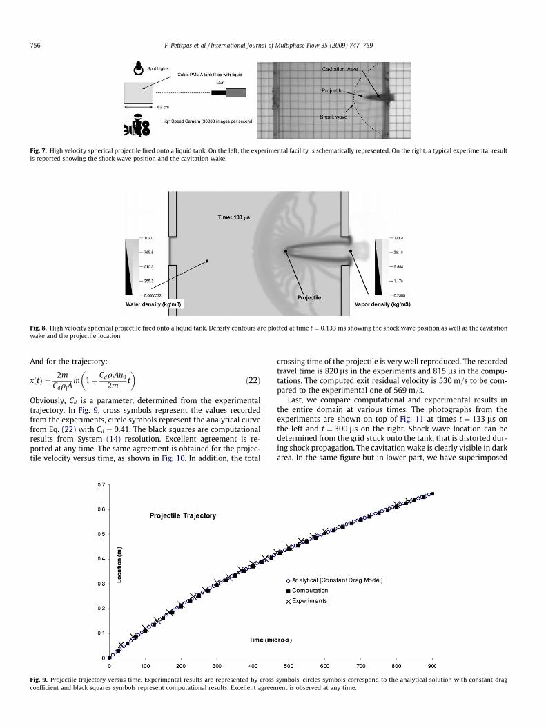
Fig. 7. High velocity spherical projectile fired onto a liquid tank. On the left, the experimental facility is schematically represented. On the right, a typical experimental resultis reported showing the shock wave position and the cavitation wake.

Fig. 8. High velocity spherical projectile fired onto a liquid tank. Density contours are plotted at time t ¼ 0:133 ms showing the shock wave position as well as the cavitationwake and the projectile location.


And for the trajectory:

xðtÞ ¼ 2mCdqlA

ln 1þ CdqlAu0

2mt

� �ð22Þ

Obviously, Cd is a parameter, determined from the experimentaltrajectory. In Fig. 9, cross symbols represent the values recordedfrom the experiments, circle symbols represent the analytical curvefrom Eq. (22) with Cd ¼ 0:41. The black squares are computationalresults from System (14) resolution. Excellent agreement is re-ported at any time. The same agreement is obtained for the projec-tile velocity versus time, as shown in Fig. 10. In addition, the total

Fig. 9. Projectile trajectory versus time. Experimental results are represented by crosscoefficient and black squares symbols represent computational results. Excellent agreem

crossing time of the projectile is very well reproduced. The recordedtravel time is 820 ls in the experiments and 815 ls in the compu-tations. The computed exit residual velocity is 530 m=s to be com-pared to the experimental one of 569 m=s.

Last, we compare computational and experimental results inthe entire domain at various times. The photographs from theexperiments are shown on top of Fig. 11 at times t ¼ 133 ls onthe left and t ¼ 300 ls on the right. Shock wave location can bedetermined from the grid stuck onto the tank, that is distorted dur-ing shock propagation. The cavitation wake is clearly visible in darkarea. In the same figure but in lower part, we have superimposed

symbols, circles symbols correspond to the analytical solution with constant dragent is observed at any time.

Fig. 10. Projectile velocity versus time. The analytical constant drag model solution is shown with dash–dot lines. An error bar with 5% error around the analytical solution isshown. Computational results are shown with black squares symbols. They always stay inside the error bar of 5%).

Fig. 11. High velocity spherical projectile fired onto a liquid tank. Computational results (density contours) are superimposed with experimental photographs at timet ¼ 0:133 ms on the left and time t ¼ 0:3 ms on the right.

Fig. 12. Initial configuration for the underwater solid rocket motor computation.


Fig. 13. Rocket motor moving at high velocity underwater. Mixture density contours are shown. The cavitation pocket composed of propulsion gases and steam is clearlyvisible.


computed liquid water density contour. The shape, size and loca-tion of the cavitation pocket is in perfect agreement. The locationof the shock wave is clearly recovered too. The ejected mixturefrom the orifice also shows excellent agreement too.

4.4. Underwater missile

The last test illustrates model’s capabilities to treat interfaceswith and without phase transition. The typical situation underinterest consists in an underwater missile moving at very highvelocity. In the present simulation the solid rocket motor is rep-resented by an immersed obstacle surrounded by liquid water at

Fig. 14. Rocket motor moving at high velocity underwater. The left column corresponcontours. From top to bottom, these two variables are shown for liquid, vapor and inert gpresent. The gas ejected from the rocket nozzle fills the major part of the cavitation pockeis present. A portion of combustion gas products move upstream, in the rocket’s head d

velocity 600 m=s. Liquid water is initially at atmospheric pres-sure with a density of 1050 kg=m3. A weak volume fraction ofvapor ðav ¼ 10�3Þ is initially present into the liquid. A non-con-densable gas is ejected through the rocket nozzle. In Fig. 13,compression waves at the rocket’s head are visible and the pres-sure exceeds 2000 atm. Then the flow undergoes strong rarefac-tion waves at geometrical singularities and the pressuredecreases below the saturation pressure resulting in liquid evap-oration. Combustion gases ejected through the nozzle fill themajor part of the pocket. An aspiration phenomenon is also vis-ible in Fig. 14 where the propulsion gas moves upstream in therocket’s head direction.

ds to volume fraction contours, while, the right one corresponds to mass fractionas, respectively. The black color is used in the regions where the considered fluid ist. Nevertheless, at the pocket boundary a small mass fraction of vapor (less than 0.1)irection.


5. Conclusions

A relatively simple compared to the problem complexity andefficient formulation has been built in order to deal with interfaces,metastable liquids, cavitating flows and shocks in several spacedimensions. The simplicity is due to a flow model valid at eachpoint location, whose resolution is possible with a single numericalstrategy. Examples with interfaces of simple contact and evaporat-ing fronts are shown and validated against exact solutions andexperimental data.

In the future it is planned to investigate capillary effects cou-pling (Perigaud and Saurel, 2005) in this diffuse interface theoryto deal with the direct numerical simulation of evaporating andflashing bubbles and drops.

References

Baer, M., Nunziato, J., 1986. A two-phase mixture theory for the deflagration-to-detonation transition (DDT) in reactive granular materials. Int. J. MultiphaseFlows 12, 861–889.

Chinnayya, A., Daniel, E., Saurel, R., 2004. Computation of detonation waves inheterogeneous energetic materials. J. Comput. Phys. 196, 490–538.

Kapila, A., Menikoff, R., Bdzil, J., Son, S., Stewart, D., 2001. Two-phase modeling of DDTin granular materials: reduced equations. Phys. Fluids 13, 3002–3024.

Le Metayer, O., Massoni, J., Saurel, R., 2004. Elaborating equations of state of a liquidand its vapor for two-phase flow models. Int. J. Therm. Sci. 43, 265–276.

Lecysyn, N., Dandrieux, A., Heymes, F., Slangen, P., Munier, L., Lapebie, E., Le Gallic, C.,Dusserre, G., 2008. Preliminary study of ballistic impact on an industrial tank:projectile velocity decay. J. Loss Prevent. Process Indust. 21, 627–634.

Liu, T., Khoo, B., Xie, W., 2004. Isentropic one-fluid modelling of unsteady cavitatingflow. J. Comput. Phys. 201, 80–108.

Menikoff, R., Plohr, B., 1989. The Riemann problem for fluid flow of real materials.Rev. Mod. Phys. 61, 75–130.

Murrone, A., Guillard, H., 2005. A five equations reduced model for compressibletwo-phase flow problems. J. Comput. Phys. 202, 664–698.

Perigaud, G., Saurel, R., 2005. A compressible flow model with capillary effects. J.Comput. Phys. 209, 139–178.

Petitpas, F., Franquet, E., Saurel, R., Le Metayer, O., 2007. A relaxation-projectionmethod for compressible flows. Part 2: artificial heat exchange for multiphaseshocks. J. Comput. Phys. 225, 2214–2248.

Saurel, R., Abgrall, R., 1999. A multiphase Godunov method for compressiblemultifluid and multiphase flows. J. Comput. Phys. 150, 425–467.

Saurel, R., Gavrilyuk, S., Renaud, F., 2003. A multiphase model with internal degrees offreedom: application to shock–bubble interaction. J. Fluid Mech. 495, 283–321.

Saurel, R., Petitpas, F., Abgrall, R., 2008. Modelling phase transition in metastableliquids: application to cavitating and flashing flows. J. Fluid Mech. 607, 313–350.

Saurel, R., Petitpas, F., Berry, R., 2009. Simple and efficient relaxation methods forinterfaces separating compressible fluids, cavitating flows and shocks inmultiphase mixtures. J. Comput. Phys. 228, 1678–1712.

Simoes-Moreira, J., Shepherd, J., 1999. Evaporation waves in superheated dodecane.J. Fluid Mech. 382, 63–86.

Wood, A., 1930. A Textbook of Sound. G. Bell and Sons Ltd., London.

Diffuse interface model for high speed cavitating underwater systems

Documents

Transcript of Diffuse interface model for high speed cavitating underwater systems