![Biological and molecular diagnosis of three different symptoms of TYLCV-disease [tomato yellow leaf curl virus] in open field](https://static.fdokumen.com/doc/165x107/63153b705cba183dbf07e655/biological-and-molecular-diagnosis-of-three-different-symptoms-of-tylcv-disease.jpg)
Diagnosis and control using multiple models. Application to a biological reactor
62
Diagnosis and control using multiple models. Application to a biological reactor Jos´ e Ragot Institut National Polytechnique de Lorraine (INPL) Centre de Recherche en Automatique de Nancy, France (CNRS) International Symposium on Advanced Control of Industrial Processes, Hangzhou, May 23-26, 2011 1/33
-
Upload
inpl-nancy -
Category
Documents
-
view
0 -
download
0
Transcript of Diagnosis and control using multiple models. Application to a biological reactor

Diagnosis and control using multiple models.
Application to a biological reactor
Jose Ragot
Institut National Polytechnique de Lorraine (INPL)Centre de Recherche en Automatique de Nancy, France (CNRS)
International Symposium on Advanced Control of IndustrialProcesses, Hangzhou, May 23-26, 2011
1/33

Introduction. Study background
◮ Processes related to environmentalAir pollution, water pollution, watertreatment plants, water distributionsystems, runoff, rainfall . . .
◮ Diagnostic of systemsValidation of measurements, detectionand fault location, fault tolerantcontrol. . .
◮ Models of environmental processesPhenomena are difficult to model,perturbations with critical effects,concentration of species difficult tomeasure. . .
◮ Fundamental issuesEnvironmental protection, protection ofcitizen . . .
2/33

1. A short presentation about our lab
The ≪ Centre de Recherche enAutomatique deNancy ≫ (Automatic Control) isa Research Centre funded by the”Centre National de laRecherche Scientifique (CNRS)”and two universities in Nancy :UHP (Universite Henri Poincare)and INPL (Institut NationalPolytechnique de Lorraine).
The CRAN was set up in Nancy (France) in 1980.It totals 200 persons. The research activitiesconcentrate on 5 principal themes :- Systems Observation and Control- System Identification and Signal Processing- Dependability and System Diagnosis- Health Engineering- Ambient Manufacturing Systems.
Dependability and
System Diagnosis
Automatic Control:
System Observation
and Control
System
Identification and
Signal Processing
Health
Engineering
Ambiant
Manufacturing
Systems
3/33

Plan
1 Introduction
2 Theoretical backgroundStructure of a multi-modelSeparating fast and slow modesA multimodel based observerController design
3 Application to a biological reactorModel of a biological reactorSlow and fast modes of functionningObserver
4 Conclusion
4/33
1. Structure of a multimodel
5/33
1.1 - How to obtain a multi-model ?
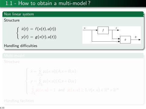
Non linear system
Structure
{
x(t) = f (x(t),u(t))
y(t) = g(x(t),u(t))
f
g
u x
y
Handling difficulties
Multi-model
Structure
x =r
∑i=1
µi(x ,u)(Aix+Biu )
y =r
∑i=1
µi (x ,u)(Cix+Diu )
r
∑i=1
µi (x ,u) = 1 and µi (x ,u)≥ 0,∀(x ,u) ∈ Rn×R
m
Handling facilities
6/33
1.1 - How to obtain a multi-model ?
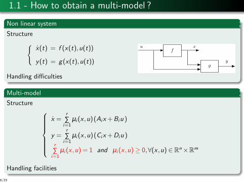
Non linear system
Structure
{
x(t) = f (x(t),u(t))
y(t) = g(x(t),u(t))
f
g
u x
y
Handling difficulties
Multi-model
Structure
x =r
∑i=1
µi(x ,u)(Aix+Biu )
y =r
∑i=1
µi (x ,u)(Cix+Diu )
r
∑i=1
µi (x ,u) = 1 and µi (x ,u)≥ 0,∀(x ,u) ∈ Rn×R
m
Handling facilities
6/33
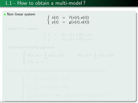
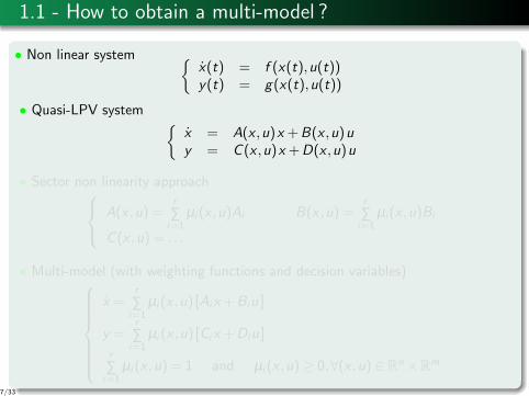
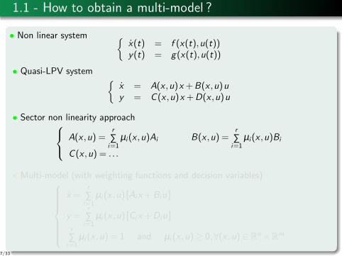
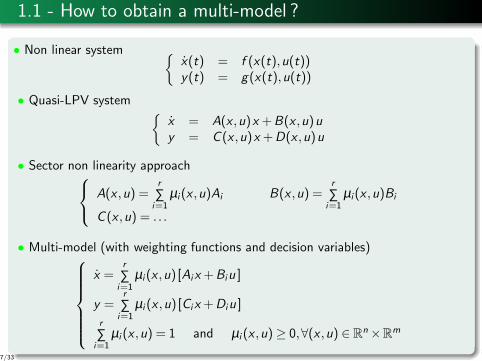
1.1 - How to obtain a multi-model ?
• Non linear system{
x(t) = f (x(t),u(t))y(t) = g(x(t),u(t))
• Quasi-LPV system{
x = A(x ,u)x +B(x ,u)uy = C (x ,u)x +D(x ,u)u
• Sector non linearity approach
A(x ,u) =r
∑i=1
µi(x ,u)Ai B(x ,u) =r
∑i=1
µi(x ,u)Bi
C (x ,u) = . . .
• Multi-model (with weighting functions and decision variables)
x =r
∑i=1
µi(x ,u) [Aix+Biu ]
y =r
∑i=1
µi (x ,u) [Cix+Diu ]
r
∑i=1
µi (x ,u) = 1 and µi (x ,u)≥ 0,∀(x ,u) ∈ Rn×R
m
7/33
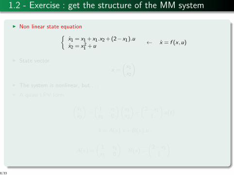
1.2 - Exercise : get the structure of the MM system
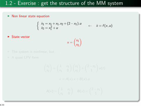
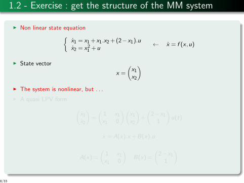
◮ Non linear state equation
{
x1 = x1+x1.x2+(2−x1).ux2 = x21 +u
← x = f (x ,u)
◮ State vector
x =
(
x1x2
)
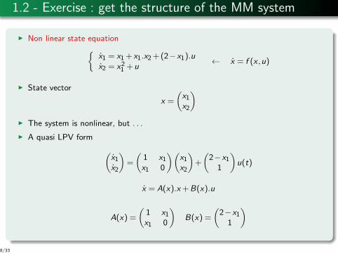
◮ The system is nonlinear, but . . .
◮ A quasi LPV form
(
x1x2
)
=
(
1 x1x1 0
)(
x1x2
)
+
(
2−x11
)
u(t)
x = A(x).x+B(x).u
A(x) =
(
1 x1x1 0
)
B(x) =
(
2−x11
)
8/33
1.2 - Exercise : get the structure of the MM system
◮ Non linear state equation
{
x1 = x1+x1.x2+(2−x1).ux2 = x21 +u
← x = f (x ,u)
◮ State vector
x =
(
x1x2
)
◮ The system is nonlinear, but . . .
◮ A quasi LPV form
(
x1x2
)
=
(
1 x1x1 0
)(
x1x2
)
+
(
2−x11
)
u(t)
x = A(x).x+B(x).u
A(x) =
(
1 x1x1 0
)
B(x) =
(
2−x11
)
8/33
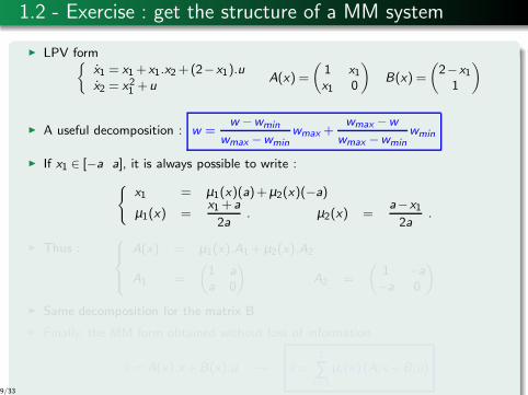
1.2 - Exercise : get the structure of a MM system
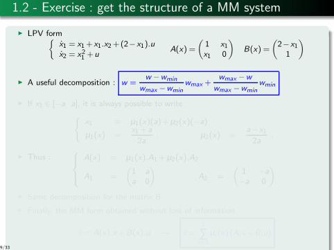
◮ LPV form{
x1 = x1+x1.x2+(2−x1).ux2 = x21 +u
A(x) =
(
1 x1x1 0
)
B(x) =
(
2−x11
)
◮ A useful decomposition : w =w −wmin
wmax −wminwmax +
wmax −w
wmax −wminwmin
◮ If x1 ∈ [−a a], it is always possible to write :
{
x1 = µ1(x)(a)+µ2(x)(−a)
µ1(x) =x1+a
2a. µ2(x) =
a−x1
2a.
◮ Thus :
A(x) = µ1(x).A1+µ2(x).A2
A1 =
(
1 a
a 0
)
A2 =
(
1 −a
−a 0
)
◮ Same decomposition for the matrix B
◮ Finally, the MM form obtained without loss of information :
x = A(x).x+B(x).u → x =2
∑i=1
µi (x)(Aix+Biu)
9/33
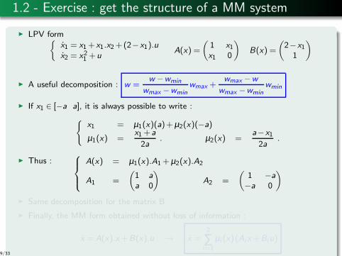
1.2 - Exercise : get the structure of a MM system
◮ LPV form{
x1 = x1+x1.x2+(2−x1).ux2 = x21 +u
A(x) =
(
1 x1x1 0
)
B(x) =
(
2−x11
)
◮ A useful decomposition : w =w −wmin
wmax −wminwmax +
wmax −w
wmax −wminwmin
◮ If x1 ∈ [−a a], it is always possible to write :
{
x1 = µ1(x)(a)+µ2(x)(−a)
µ1(x) =x1+a
2a. µ2(x) =
a−x1
2a.
◮ Thus :
A(x) = µ1(x).A1+µ2(x).A2
A1 =
(
1 a
a 0
)
A2 =
(
1 −a
−a 0
)
◮ Same decomposition for the matrix B
◮ Finally, the MM form obtained without loss of information :
x = A(x).x+B(x).u → x =2
∑i=1
µi (x)(Aix+Biu)
9/33
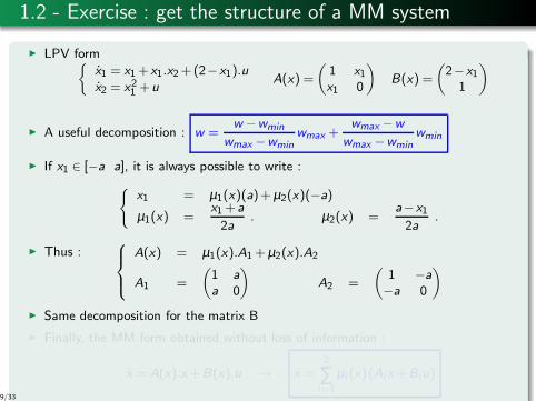
1.2 - Exercise : get the structure of a MM system
◮ LPV form{
x1 = x1+x1.x2+(2−x1).ux2 = x21 +u
A(x) =
(
1 x1x1 0
)
B(x) =
(
2−x11
)
◮ A useful decomposition : w =w −wmin
wmax −wminwmax +
wmax −w
wmax −wminwmin
◮ If x1 ∈ [−a a], it is always possible to write :
{
x1 = µ1(x)(a)+µ2(x)(−a)
µ1(x) =x1+a
2a. µ2(x) =
a−x1
2a.
◮ Thus :
A(x) = µ1(x).A1+µ2(x).A2
A1 =
(
1 a
a 0
)
A2 =
(
1 −a
−a 0
)
◮ Same decomposition for the matrix B
◮ Finally, the MM form obtained without loss of information :
x = A(x).x+B(x).u → x =2
∑i=1
µi (x)(Aix+Biu)
9/33
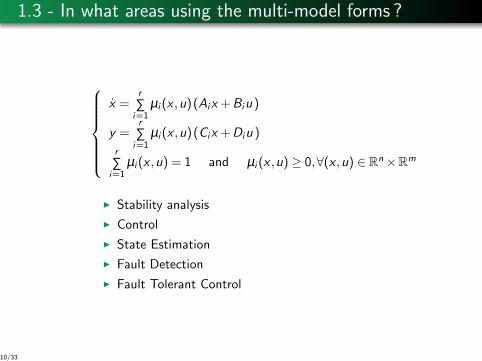
1.3 - In what areas using the multi-model forms ?
x =r
∑i=1
µi (x ,u)(Aix +Biu )
y =r
∑i=1
µi(x ,u)(Cix +Diu )
r
∑i=1
µi(x ,u) = 1 and µi (x ,u)≥ 0,∀(x ,u) ∈Rn×R
m
◮ Stability analysis
◮ Control
◮ State Estimation
◮ Fault Detection
◮ Fault Tolerant Control
10/33
2. Separating fast and slow
modes
11/33

2.1 - Singular systems
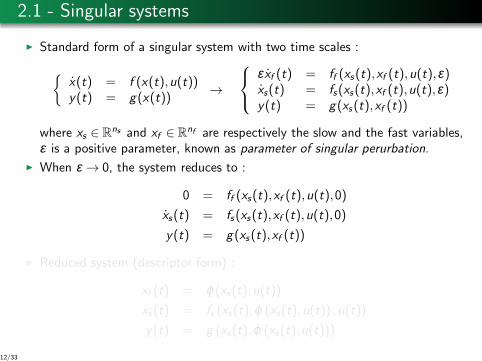
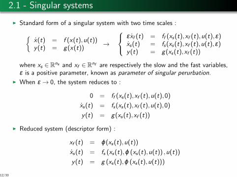
◮ Standard form of a singular system with two time scales :
{
x(t) = f (x(t),u(t))y(t) = g(x(t))
→
ε xf (t) = ff (xs(t),xf (t),u(t),ε)xs(t) = fs(xs(t),xf (t),u(t),ε)y(t) = g(xs(t),xf (t))
where xs ∈ Rns and xf ∈ R
nf are respectively the slow and the fast variables,ε is a positive parameter, known as parameter of singular perurbation.
◮ When ε → 0, the system reduces to :
0 = ff (xs(t),xf (t),u(t),0)
xs(t) = fs(xs(t),xf (t),u(t),0)
y(t) = g(xs(t),xf (t))
◮ Reduced system (descriptor form) :
xf (t) = ϕ(xs(t),u(t))xs(t) = fs (xs(t),ϕ (xs(t),u(t)) ,u(t))
y(t) = g (xs(t),ϕ (xs(t),u(t)))
12/33
2.1 - Singular systems
◮ Standard form of a singular system with two time scales :
{
x(t) = f (x(t),u(t))y(t) = g(x(t))
→
ε xf (t) = ff (xs(t),xf (t),u(t),ε)xs(t) = fs(xs(t),xf (t),u(t),ε)y(t) = g(xs(t),xf (t))
where xs ∈ Rns and xf ∈ R
nf are respectively the slow and the fast variables,ε is a positive parameter, known as parameter of singular perurbation.
◮ When ε → 0, the system reduces to :
0 = ff (xs(t),xf (t),u(t),0)
xs(t) = fs(xs(t),xf (t),u(t),0)
y(t) = g(xs(t),xf (t))
◮ Reduced system (descriptor form) :
xf (t) = ϕ(xs(t),u(t))xs(t) = fs (xs(t),ϕ (xs(t),u(t)) ,u(t))
y(t) = g (xs(t),ϕ (xs(t),u(t)))
12/33
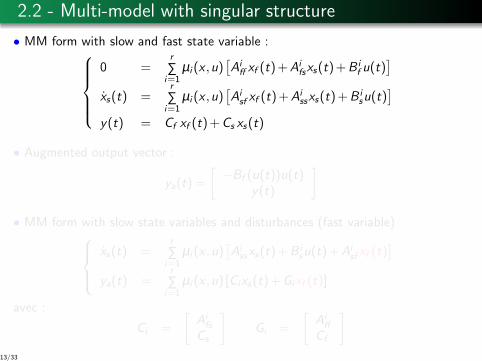
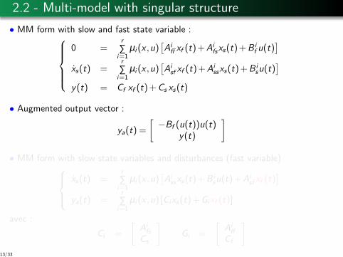
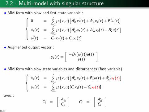
2.2 - Multi-model with singular structure
• MM form with slow and fast state variable :
0 =r
∑i=1
µi (x ,u)[
Aiff xf (t)+Ai
fsxs(t)+B if u(t)
]
xs(t) =r
∑i=1
µi (x ,u)[
Aisf xf (t)+Ai
ssxs(t)+B isu(t)
]
y(t) = Cf xf (t)+Cs xs(t)
• Augmented output vector :
ya(t) =
[
−Bf (u(t))u(t)y(t)
]
• MM form with slow state variables and disturbances (fast variable)
xs(t) =r
∑i=1
µi (x ,u)[
Aissxs(t)+B i
su(t)+Aisf xf (t)
]
ya(t) =r
∑i=1
µi (x ,u) [Cixs(t)+Gixf (t)]
avec :
Ci =
[
Aifs
Cs
]
Gi =
[
Aiff
Cf
]
13/33
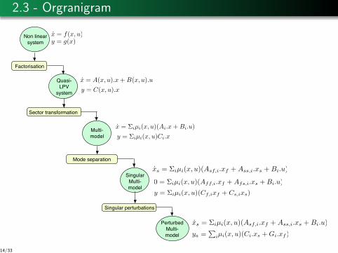
2.3 - Orgranigram
Sector transformation
Mode separation
Singular perturbations
Perturbed
Multi-
model
Singular
Multi-
model
Quasi-
LPV
system
Non linear
system
Multi-
model
Factorisation
x = f(x, u)
x = A(x, u).x+B(x, u).u
xs = Σiµi(x, u)(Asf,i.xf +Ass,i.xs +Bi.u)
xs = Σiµi(x, u)(Asf,i.xf +Ass,i.xs +Bi.u)
ya =∑
iµi(x, u)(Ci.xs +Gi.xf )
0 = Σiµi(x, u)(Aff,i.xf +Afs,i.xs +Bi.u)
y = g(x)
y = C(x, u).x
y = Σiµi(x, u)(Cf,ixf + Cs,ixs)
x = Σiµi(x, u)(Ai.x+Bi.u)
y = Σiµi(x, u)Ci.x
14/33
3. Observer and control
using a multimodel
15/33
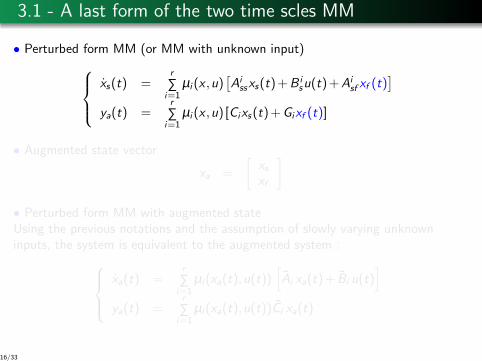
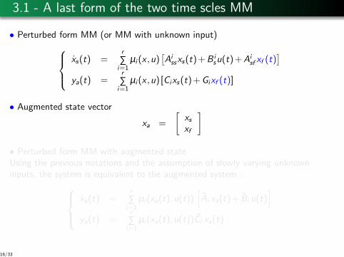
3.1 - A last form of the two time scles MM
• Perturbed form MM (or MM with unknown input)
xs(t) =r
∑i=1
µi (x ,u)[
Aissxs(t)+B i
su(t)+Aisf xf (t)
]
ya(t) =r
∑i=1
µi (x ,u) [Cixs(t)+Gixf (t)]
• Augmented state vector
xa =
[
xsxf
]
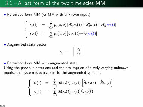
• Perturbed form MM with augmented stateUsing the previous notations and the assumption of slowly varying unknowninputs, the system is equivalent to the augmented system :
xa(t) =r
∑i=1
µi(xa(t),u(t))[
Ai xa(t)+ Bi u(t)]
ya(t) =r
∑i=1
µi(xa(t),u(t))Ci xa(t)
16/33
3.1 - A last form of the two time scles MM
• Perturbed form MM (or MM with unknown input)
xs(t) =r
∑i=1
µi (x ,u)[
Aissxs(t)+B i
su(t)+Aisf xf (t)
]
ya(t) =r
∑i=1
µi (x ,u) [Cixs(t)+Gixf (t)]
• Augmented state vector
xa =
[
xsxf
]
• Perturbed form MM with augmented stateUsing the previous notations and the assumption of slowly varying unknowninputs, the system is equivalent to the augmented system :
xa(t) =r
∑i=1
µi(xa(t),u(t))[
Ai xa(t)+ Bi u(t)]
ya(t) =r
∑i=1
µi(xa(t),u(t))Ci xa(t)
16/33

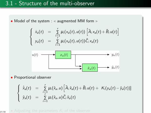
3.1 - Structure of the multi-observer
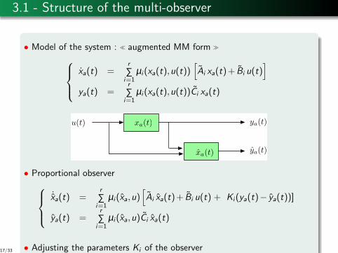
• Model of the system : ≪ augmented MM form ≫
xa(t) =r
∑i=1
µi(xa(t),u(t))[
Ai xa(t)+ Bi u(t)]
ya(t) =r
∑i=1
µi(xa(t),u(t))Ci xa(t)
ya(t)xa(t)
xa(t)u(t) ya(t)
• Proportional observer
˙xa(t) =r
∑i=1
µi(xa,u)[
Ai xa(t)+ Bi u(t) + Ki(ya(t)− ya(t))]
ya(t) =r
∑i=1
µi(xa,u)Ci xa(t)
• Adjusting the parameters Ki of the observer17/33
3.1 - Structure of the multi-observer
• Model of the system : ≪ augmented MM form ≫
xa(t) =r
∑i=1
µi(xa(t),u(t))[
Ai xa(t)+ Bi u(t)]
ya(t) =r
∑i=1
µi(xa(t),u(t))Ci xa(t)
ya(t)xa(t)
xa(t)u(t) ya(t)
• Proportional observer
˙xa(t) =r
∑i=1
µi(xa,u)[
Ai xa(t)+ Bi u(t) + Ki(ya(t)− ya(t))]
ya(t) =r
∑i=1
µi(xa,u)Ci xa(t)
• Adjusting the parameters Ki of the observer17/33
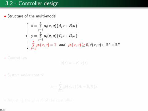
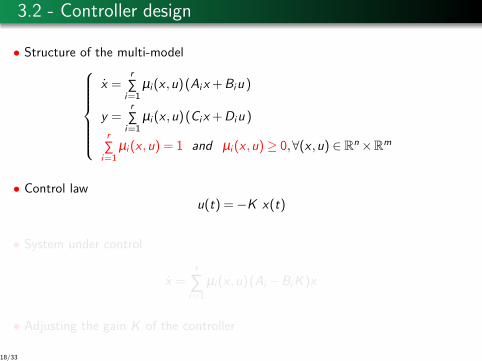
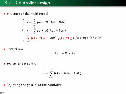
3.2 - Controller design
• Structure of the multi-model
x =r
∑i=1
µi(x ,u)(Aix+Biu )
y =r
∑i=1
µi (x ,u)(Cix+Diu )
r
∑i=1
µi (x ,u) = 1 and µi (x ,u)≥ 0,∀(x ,u) ∈ Rn×R
m
• Control lawu(t) =−K x(t)
• System under control
x =r
∑i=1
µi(x ,u)(Ai −BiK )x
• Adjusting the gain K of the controller
18/33
3.2 - Controller design
• Structure of the multi-model
x =r
∑i=1
µi(x ,u)(Aix+Biu )
y =r
∑i=1
µi (x ,u)(Cix+Diu )
r
∑i=1
µi (x ,u) = 1 and µi (x ,u)≥ 0,∀(x ,u) ∈ Rn×R
m
• Control lawu(t) =−K x(t)
• System under control
x =r
∑i=1
µi(x ,u)(Ai −BiK )x
• Adjusting the gain K of the controller
18/33

3.2 - Controller design
• Structure of the multi-model
x =r
∑i=1
µi(x ,u)(Aix+Biu )
y =r
∑i=1
µi (x ,u)(Cix+Diu )
r
∑i=1
µi (x ,u) = 1 and µi (x ,u)≥ 0,∀(x ,u) ∈ Rn×R
m
• Control lawu(t) =−K x(t)
• System under control
x =r
∑i=1
µi(x ,u)(Ai −BiK )x
• Adjusting the gain K of the controller
18/33
3.2 - Controller design
• Structure of the multi-model
x =r
∑i=1
µi(x ,u)(Aix+Biu )
y =r
∑i=1
µi (x ,u)(Cix+Diu )
r
∑i=1
µi (x ,u) = 1 and µi (x ,u)≥ 0,∀(x ,u) ∈ Rn×R
m
• Control lawu(t) =−K x(t)
• System under control
x =r
∑i=1
µi(x ,u)(Ai −BiK )x
• Adjusting the gain K of the controller
18/33

2. Application to a biological
reactor
19/33

4.1 - Flowsheet
Bioreactor
Air
Clarifier
Effluent
Recycling sludge
Feed qin qout
qwqR Wasted sludge
qa
Figure: Diagram of actived sludge wastewater treatment
SNOXA XHWaster water
Biomass
Air
Ammoniumcompounds
Solublecarbone
Waster water
Biomass
NitritesNitrates
Solublecarbone
Nitrogen gas
SS
SSSNH
SO
Figure: Reactions in nitrogen removal20/33
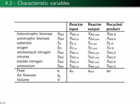
4.2 - Characteristic variables
Reactor Reactor Recycled
input output product
heterotrophic biomass XBH XBH ,in XBH ,out XBH ,R
autotrophic biomass XBH XBA,in XBA,out XBA,R
substrate SS SS,in SS,out SS,Roxygen SO SO,in SO,out SO,R
ammoniacal nitrogen SNH SNH ,in SNH ,out SNH ,R
nitrates SNO SNO,in SNO,out SNO,R
soluble nitrogen SND SND,in SND,out SND,R
ammonium SNH SNH ,in SNH ,out SNH ,R
Feed q qin qout qRAir flowrate qaVolume V
21/33
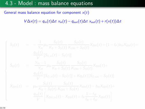
4.3 - Model : mass balance equations
General mass balance equation for component x(t)
V∆x(t) = qin(t)∆t xin(t)−qout(t)∆t xout(t)+ r(x(t))∆t
SS (t) = −1
YH
µH
SS (t)
KS +SS(t)
SO(t)
KOH +SO(t)XBH(t)+ (1− fP)bHXBH(t)+
qin(t)
V[SS,in(t)−SS(t)]
SO(t) =YH − 1
YH
µH
SS (t)
KS +SS(t)
SO(t)
KOH +SO(t)XBH(t)+
qin(t)
V[SO,in(t)−SO(t)]+Kqa(t) [SO,sat −SO(t)]
XBH(t) = µH
SS (t)
KS +SS(t)
SO(t)
KOH +SO(t)XBH(t)−bHXBH(t)+
qin(t)
V
[
XBH ,in(t)−XBH(t)+ fR1− fW
fR + fWXBH(t)
]
22/33
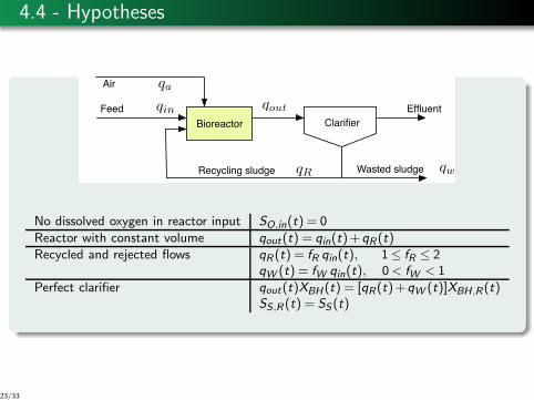
4.4 - Hypotheses
Bioreactor
Air
Clarifier
Effluent
Recycling sludge
Feed qin qout
qwqR Wasted sludge
qa
No dissolved oxygen in reactor input SO,in(t) = 0
Reactor with constant volume qout(t) = qin(t)+qR (t)
Recycled and rejected flows qR (t) = fR qin(t), 1≤ fR ≤ 2qW (t) = fW qin(t), 0< fW < 1
Perfect clarifier qout(t)XBH (t) = [qR(t)+qW (t)]XBH ,R (t)SS,R (t) = SS(t)
23/33
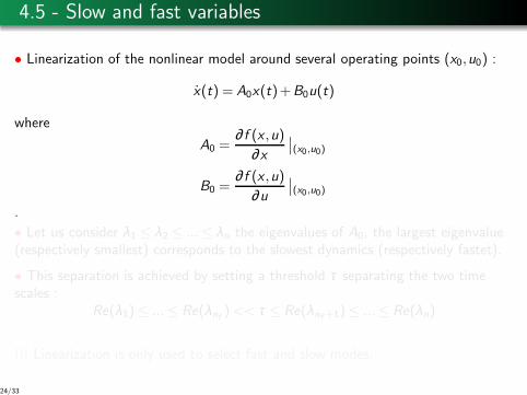
4.5 - Slow and fast variables
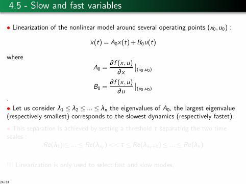
• Linearization of the nonlinear model around several operating points (x0,u0) :
x(t) = A0x(t)+B0u(t)
where
A0 =∂ f (x ,u)
∂x∣
∣
(x0,u0)
B0 =∂ f (x ,u)
∂u∣
∣
(x0,u0)
.
• Let us consider λ1 ≤ λ2 ≤ ...≤ λn the eigenvalues of A0, the largest eigenvalue(respectively smallest) corresponds to the slowest dynamics (respectively fastet).
• This separation is achieved by setting a threshold τ separating the two timescales :
Re(λ1)≤ ...≤ Re(λnf )<< τ ≤ Re(λnf +1)≤ ...≤ Re(λn)
!!! Linearization is only used to select fast and slow modes,
24/33
4.5 - Slow and fast variables
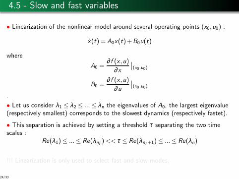
• Linearization of the nonlinear model around several operating points (x0,u0) :
x(t) = A0x(t)+B0u(t)
where
A0 =∂ f (x ,u)
∂x∣
∣
(x0,u0)
B0 =∂ f (x ,u)
∂u∣
∣
(x0,u0)
.
• Let us consider λ1 ≤ λ2 ≤ ...≤ λn the eigenvalues of A0, the largest eigenvalue(respectively smallest) corresponds to the slowest dynamics (respectively fastet).
• This separation is achieved by setting a threshold τ separating the two timescales :
Re(λ1)≤ ...≤ Re(λnf )<< τ ≤ Re(λnf +1)≤ ...≤ Re(λn)
!!! Linearization is only used to select fast and slow modes,
24/33
4.5 - Slow and fast variables
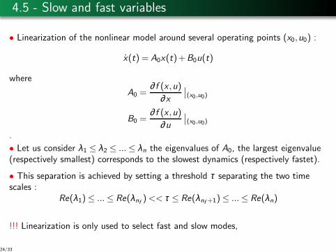
• Linearization of the nonlinear model around several operating points (x0,u0) :
x(t) = A0x(t)+B0u(t)
where
A0 =∂ f (x ,u)
∂x∣
∣
(x0,u0)
B0 =∂ f (x ,u)
∂u∣
∣
(x0,u0)
.
• Let us consider λ1 ≤ λ2 ≤ ...≤ λn the eigenvalues of A0, the largest eigenvalue(respectively smallest) corresponds to the slowest dynamics (respectively fastet).
• This separation is achieved by setting a threshold τ separating the two timescales :
Re(λ1)≤ ...≤ Re(λnf )<< τ ≤ Re(λnf +1)≤ ...≤ Re(λn)
!!! Linearization is only used to select fast and slow modes,
24/33
4.5 - Slow and fast variables
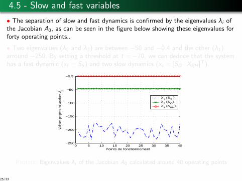
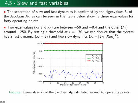
• The separation of slow and fast dynamics is confirmed by the eigenvalues λi ofthe Jacobian A0, as can be seen in the figure below showing these eigenvalues forforty operating points..
• Two eigenvalues (λ2 and λ3) are between −50 and −0.4 and the other (λ1)arround −250. By setting a threshold at τ =−70, we can deduce that the systemhas a fast dynamic (xf = SS) and two slow dynamics (xs = [SO XBH ]
T ).
0 5 10 15 20 25 30 35 40−250
−200
−150
−100
−50
−0.5
Points de fonctionnement
Valeu
rs p
ropr
es d
u jac
obien
A0
λ1 (S
S )
λ2 (S
O)
λ3 (X
BH)
Figure: Eigenvalues λi of the Jacobian A0 calculated around 40 operating points
25/33
4.5 - Slow and fast variables
• The separation of slow and fast dynamics is confirmed by the eigenvalues λi ofthe Jacobian A0, as can be seen in the figure below showing these eigenvalues forforty operating points..
• Two eigenvalues (λ2 and λ3) are between −50 and −0.4 and the other (λ1)arround −250. By setting a threshold at τ =−70, we can deduce that the systemhas a fast dynamic (xf = SS) and two slow dynamics (xs = [SO XBH ]
T ).
0 5 10 15 20 25 30 35 40−250
−200
−150
−100
−50
−0.5
Points de fonctionnement
Valeu
rs p
ropr
es d
u jac
obien
A0
λ1 (S
S )
λ2 (S
O)
λ3 (X
BH)
Figure: Eigenvalues λi of the Jacobian A0 calculated around 40 operating points
25/33
4.6 - How to get the multi-model structure ?
SS (t) =−1
YH
µH
SS (t)
KS +SS (t)
SO(t)
KOH +SO(t)XBH (t)+(1− fP )bHXBH (t)+
qin(t)
V
[
SS,in(t)−SS (t)]
SO(t) =YH −1
YH
µH
SS (t)
KS +SS (t)
SO (t)
KOH +SO(t)XBH (t)+
qin(t)
V
[
SO,in(t)−SO (t)]
+Kqa(t)[
SO,sat −
XBH (t) = µH
SS (t)
KS +SS (t)
SO(t)
KOH +SO(t)XBH (t)−bHXBH (t)+
qin(t)
V
[
XBH,in(t)−XBH (t)+ fR1− fW
fR + f
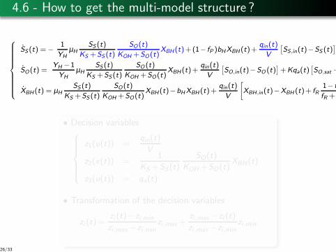
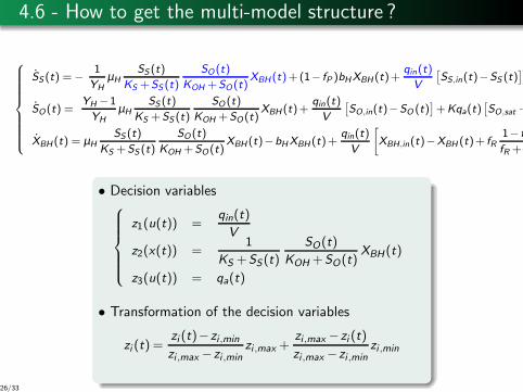
• Decision variables
z1(u(t)) =qin(t)
V
z2(x(t)) =1
KS +SS(t)
SO(t)
KOH +SO(t)XBH (t)
z3(u(t)) = qa(t)
• Transformation of the decision variables
zi (t) =zi (t)−zi ,min
zi ,max −zi ,minzi ,max +
zi ,max −zi (t)
zi ,max −zi ,minzi ,min
26/33
4.6 - How to get the multi-model structure ?
SS (t) =−1
YH
µH
SS (t)
KS +SS (t)
SO(t)
KOH +SO(t)XBH (t)+(1− fP )bHXBH (t)+
qin(t)
V
[
SS,in(t)−SS (t)]
SO(t) =YH −1
YH
µH
SS (t)
KS +SS (t)
SO (t)
KOH +SO(t)XBH (t)+
qin(t)
V
[
SO,in(t)−SO (t)]
+Kqa(t)[
SO,sat −
XBH (t) = µH
SS (t)
KS +SS (t)
SO(t)
KOH +SO(t)XBH (t)−bHXBH (t)+
qin(t)
V
[
XBH,in(t)−XBH (t)+ fR1− fW
fR + f
• Decision variables
z1(u(t)) =qin(t)
V
z2(x(t)) =1
KS +SS(t)
SO(t)
KOH +SO(t)XBH (t)
z3(u(t)) = qa(t)
• Transformation of the decision variables
zi (t) =zi (t)−zi ,min
zi ,max −zi ,minzi ,max +
zi ,max −zi (t)
zi ,max −zi ,minzi ,min
26/33
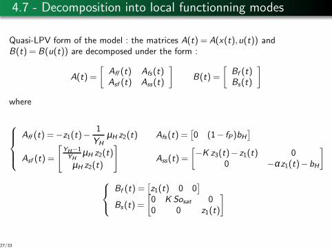
4.7 - Decomposition into local functionning modes
Quasi-LPV form of the model : the matrices A(t) = A(x(t),u(t)) andB(t) = B(u(t)) are decomposed under the form :
A(t) =
[
Aff (t) Afs(t)Asf (t) Ass(t)
]
B(t) =
[
Bf (t)Bs(t)
]
where
Aff (t) =−z1(t)−1
YH
µH z2(t) Afs(t) =[
0 (1− fP)bH]
Asf (t) =
[
YH−1YH
µH z2(t)
µH z2(t)
]
Ass(t) =
[
−K z3(t)− z1(t) 00 −αz1(t)−bH
]
Bf (t) =[
z1(t) 0 0]
Bs(t) =
[
0 K Sosat 00 0 z1(t)
]
27/33
4.7 - Decomposition into local functionning modes
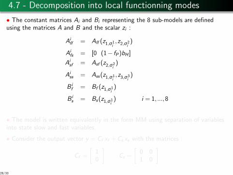
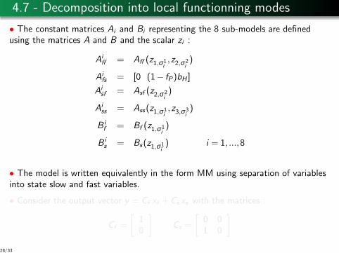
• The constant matrices Ai and Bi representing the 8 sub-models are definedusing the matrices A and B and the scalar zi :
Aiff = Aff (z1,σ1
i,z2,σ2
i)
Aifs = [0 (1− fP)bH ]
Aisf = Asf (z2,σ2
i)
Aiss = Ass(z1,σ1
i,z3,σ3
i)
B if = Bf (z1,σ1
i)
B is = Bs(z1,σ1
i) i = 1, ...,8
• The model is written equivalently in the form MM using separation of variablesinto state slow and fast variables.
• Consider the output vector y = Cf xf +Cs xs with the matrices :
Cf =
[
10
]
Cs =
[
0 01 0
]
28/33
4.7 - Decomposition into local functionning modes
• The constant matrices Ai and Bi representing the 8 sub-models are definedusing the matrices A and B and the scalar zi :
Aiff = Aff (z1,σ1
i,z2,σ2
i)
Aifs = [0 (1− fP)bH ]
Aisf = Asf (z2,σ2
i)
Aiss = Ass(z1,σ1
i,z3,σ3
i)
B if = Bf (z1,σ1
i)
B is = Bs(z1,σ1
i) i = 1, ...,8
• The model is written equivalently in the form MM using separation of variablesinto state slow and fast variables.
• Consider the output vector y = Cf xf +Cs xs with the matrices :
Cf =
[
10
]
Cs =
[
0 01 0
]
28/33
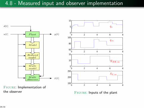
4.8 - Measured input and observer implementation
u(t) y(t)
x(t)
d(t)
Plant
Multi
observerMulti
Reduced
model
Model
model
Figure: Implementation ofthe observer
0 2 4 6 80
5
10
qa
0 2 4 6 860
80
100qin
0 2 4 6 85
10
15
XBH,in
0 2 4 6 8150
200
250SS, in
Figure: Inputs of the plant
29/33
4.9 - State observer
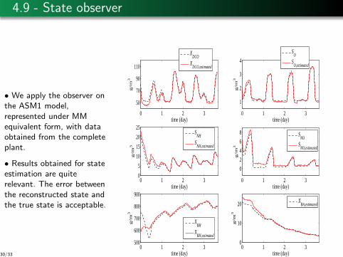
• We apply the observer onthe ASM1 model,represented under MMequivalent form, with dataobtained from the completeplant.
• Results obtained for stateestimation are quiterelevant. The error betweenthe reconstructed state andthe true state is acceptable.
0 1 2 3
50
70
90
110
time (day)
g/m
3
0 1 2 3
1
2
3
4
time (day)
g/m
3
0 1 2 30
5
10
15
20
25
time (day)
g/m
3
0 1 2 3
0
2
4
6
8
time (day)
g/m
3
0 1 2 3500
600
700
800
900
time (day)
g/m
3
0 1 2 30
10
20
time (day)
g/m
3
XDCO
XDCO,estimated
SNO
SNO,estimated
XBH
XBH,estimated
SNH
SNH,estimated
SO
SO,estimated
XBA,estimated
30/33
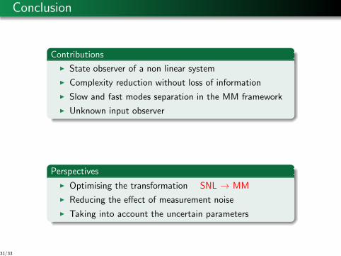
Conclusion
Contributions
◮ State observer of a non linear system
◮ Complexity reduction without loss of information
◮ Slow and fast modes separation in the MM framework
◮ Unknown input observer
Perspectives
◮ Optimising the transformation SNL → MM
◮ Reducing the effect of measurement noise
◮ Taking into account the uncertain parameters
31/33

Thank you for your attention
Place Stanislas in Nancy
32/33