water

Article

Dew Point Temperature Estimation: Application ofArtificial Intelligence Model Integrated withNature-Inspired Optimization Algorithms

Sujay Raghavendra Naganna 1,2 , Paresh Chandra Deka 3,∗ , Mohammad Ali Ghorbani 4,5,Seyed Mostafa Biazar 5 , Nadhir Al-Ansari 6 and Zaher Mundher Yaseen 7,∗

1 Department of Civil Engineering, Shri Madhwa Vadiraja Institute of Technology and Management,Bantakal-574115, Udupi, India; sujay.civil@sode-edu.in

2 Visvesvaraya Technological University, Belagavi, Karnataka 590018, India3 Department of Applied Mechanics and Hydraulics, National Institute of Technology Karnataka, Surathkal,

Mangalore-575025, India4 Department of Civil Engineering, Near East University, P.O. Box 99138, Nicosia, North Cyprus,

Mersin 10, Turkey; m_ali_ghorbani@ymail.com5 Department of Water Engineering, Faculty of Agriculture, University of Tabriz, 5166616471 Tabriz, Iran;

seyedmostafa.b@gmail.com6 Civil, Environmental and Natural Resources Engineering, Lulea University of Technology,

97187 Lulea, Sweden; nadhir.alansari@ltu.se7 Sustainable Developments in Civil Engineering Research Group, Faculty of Civil Engineering,

Ton Duc Thang University, Ho Chi Minh City, Vietnam* Correspondence: dekanitk@gmail.com (P.C.D.); yaseen@tdtu.edu.vn (Z.M.Y.)

Received: 1 February 2019; Accepted: 2 April 2019; Published: 10 April 2019�����������������

Abstract: Dew point temperature (DPT) is known to fluctuate in space and time regardless ofthe climatic zone considered. The accurate estimation of the DPT is highly significant for variousapplications of hydro and agro–climatological researches. The current research investigated thehybridization of a multilayer perceptron (MLP) neural network with nature-inspired optimizationalgorithms (i.e., gravitational search (GSA) and firefly (FFA)) to model the DPT of two climaticallycontrasted (humid and semi-arid) regions in India. Daily time scale measured weather information,such as wet bulb temperature (WBT), vapor pressure (VP), relative humidity (RH), and dew pointtemperature, was used to build the proposed predictive models. The efficiencies of the proposedhybrid MLP networks (MLP–FFA and MLP–GSA) were authenticated against standard MLP tuned bya Levenberg–Marquardt back-propagation algorithm, extreme learning machine (ELM), and supportvector machine (SVM) models. Statistical evaluation metrics such as Nash Sutcliffe efficiency(NSE), root mean square error (RMSE), and mean absolute error (MAE) were used to validatethe model efficiency. The proposed hybrid MLP models exhibited excellent estimation accuracy.The hybridization of MLP with nature-inspired optimization algorithms boosted the estimationaccuracy that is clearly owing to the tuning robustness. In general, the applied methodology showedvery convincing results for both inspected climate zones.

Keywords: dew point temperature; firefly algorithm; gravitational search algorithm; humid climate;hybrid models; nature-inspired optimization; semi-arid region

1. Introduction

Dew point temperature (DPT) is a weather condition that happens when the air is fully saturatedwith water vapor and the number of water molecules evaporating from any surface is in equilibrium

Water 2019, 11, 742; doi:10.3390/w11040742 www.mdpi.com/journal/water

Water 2019, 11, 742 2 of 17

with the number of molecules condensing [1]. Fluctuations of DPT in combination with other weatherparameters have a remarkable potential impact on regional agriculture, water supplies, and humanwell-being. In addition, it serves as an essential variable to model precipitation and frost processes.Further, DPT also influences crop yields by the spread of many pathogens through free moisture [2].Nevertheless, a slow rate of drop in the dew point temperature results in evaporative cooling [3] and,conversely, a rise in DPT intensifies the impacts of heat waves on the environment [4].

DPT has several characteristics related with atmospheric features. For instance, semi-aridenvironments sometimes experience negative dew points, when air temperatures are between 50–60◦ Fwith the relative humidity levels dropping below 10% [5]. On the other hand, dew point values inthe range of 13–20◦ F are critical and lead to cold nights with possible difficulty in keeping roomtemperatures above critical levels. Air holds very little moisture when the dew point is below zero.In dry seasons, dewfall and direct water vapor adsorption are the main mechanisms that add waterto the soil [6]. Dew recharges the soil moisture in addition to limiting evaporation from soil surfaceduring the time of dewfall.

Other climate environments, e.g., “humid zones”, especially at the coastal tropics are more likelyto experience dew points compared to arid and semi-arid regions [7]. Some coastal forests havemeasurable moisture inputs from condensation onto tall trees which drips, through fall, and someinfiltrates into soil. Seasonal weather conditions also impact an area’s dew point. Strong breezes,for example, blend diverse layers of air, containing different amounts of water vapor, thus reducing theatmosphere’s ability to form dew. Nowadays, estimation of DPT is of particular interest to researchersworking in the area of meteorology and climate. This is because it is one among weather parameters tobe considered as an input for climate change impact assessments [8]. In addition, it controls hygroscopicgrowth of aerosols, aids in estimating the height of cumulus or stratocumulus cloud bases for aviationweather forecasts, and helps in developing systems to enhance predictions of hydro–meteorologicalvariables at basin scale [9,10].

Currently, several studies exist in the field of DPT modeling using empirical equations andmachine learning (ML) models. Psychrometric charts or else the Magnus–Tetens equation were oftenused to calculate dew point temperature using weather parameters such as humidity ratio, dry bulbtemperature, saturation vapor pressure, etc. [11]. One of the earliest studies conducted on this groundby Lawrence (2005) [12], established a general mathematical relationship between the dew pointand relative humidity through simple conversion equations. The main drawback of the empiricalformulations is the limitation of the generalization application for a wide range of climatic zones.In addition, these empirical formulas are processed through a complicated procedure of determinations.Hence, a new era of application was emphasized to be implemented for the determination of DPT,through the development of soft computing models.

Over the past two decades, the implementation of the soft computing models has demonstrateda remarkable progression in various hydrological applications [13–17]. In particular, variousML models have been explored for the modeling of DPT using neural networks, support vectormachines, neurofuzzy systems, extreme learning machines, evolutionary computing models. etc.These models usually involve data of various other agro–meteorological parameters as modelinputs to estimate DPT. The neural network based on multistep time lead prediction modelstested by Shank et al. (2008) [18] was successful in predicting year-round DPT more accurately.The Levenberg–Marquardt feed-forward neural network performed better than the multilinearregression (MLR) model while estimating the hourly dew point temperature of Geraldton, a climatestation in Canada [19]. Usually, Artificial Neural Network (ANN) models are designed to targetonly one output. However, Nadig et al. (2013) [20] designed a combined ANN model (having morethan one output variable) that predicts both air temperature and DPT of a single prediction horizon,taking into account prediction anomalies. The effect of different climatic variables (sunshine hours, airtemperature, wind speed, relative humidity, and saturation vapor pressure) on daily DPT estimationwas examined by Kisi et al. (2013) [21] using different learning algorithms of neural network and

Water 2019, 11, 742 3 of 17

adaptive neural fuzzy inference systems (ANFIS). Shiri et al. (2014) [22] tested ANN and geneexpression programming (GEP) models for estimating daily DPT of a station by employing theweather data of a neighboring station and termed it as cross-station application. A generalizedregression neural network (GRNN) and multilayer perceptron (MLP) neural network using single andmultiple variable input combinations were developed by Kim et al. (2015) [23] to find the best inputcombination that estimates daily DPT with high accuracy. Recently, similar studies conducted usingextreme learning machine (ELM) [24], adaptive neurofuzzy inference system (ANFIS) [25], supportvector machine (SVM) [26], gene expression programming (GEP), and multivariate adaptive regressionsplines (MARS) [27] estimated/modeled DPT with sufficient levels of accuracy. Genetic algorithm(GA) based least square SVM and ANFIS models developed by Baghban et al. (2016) [28] predict themoist air DPT over an extensive range of relative humidity and temperature. Here, GA was employedto optimize the corresponding parameters of ANFIS and LS–SVM models. Several other investigationshave been conducted on dew point temperature prediction [21,29,30]. As a general complement overthe surveyed studies, the application of soft computing techniques revealed an excellent performancein modeling DPT.

The performance of MLP network architecture is usually dependent on settings ofhyper-parameters (number of layers, layer size, layer type), activation function for each layer,optimization algorithm, learning rate with momentum coefficient, regularization, and initializationmethods [31]. Hyper-parameters can strongly interact with each other to affect performance. On thesegrounds, multilayer perceptron neural networks are known to have some intrinsic disadvantages,such as slow convergence speed, less generalizing performance, overfitting problems, issues of localminima, and saddle points, which can trap the optimization algorithm at bad solutions [32,33].Hence, optimizing the MLP network using nature-inspired optimization algorithms can elevatethe predictability performance of the model [34].

After an extensive and thorough analysis of the existing literature, the development of hybridMLP networks was anticipated to be the feasible optimal solution to model DPT. Hence, in thepresent study, two hybrid approaches, namely the MLP neural network coupled with the gravitationalsearch and firefly optimizer algorithms (MLP–GSA and MLP–FFA) are introduced to enhance theefficiency of daily DPT estimates of semi-arid (Hyderabad) and humid (Bajpe) regions of India.The gravitational search algorithm (GSA), applied in this research, is a nature-inspired metaheuristicoptimization tool grounded on the gravitational law and mass interactions [35] and, similarly,the mathematical formulations of the firefly algorithm (FFA) are constituted on the flashing behaviorof fireflies [36]. Both of these algorithms have demonstrated their capability to search for the globaloptimum solution [37,38]. The weather information, including wet bulb temperature, relative humidity,and vapor pressure, are used as model inputs to estimate daily DPT. The performance of these hybridMLP systems, related to the estimation of daily DPT, is compared to those obtained in our previousstudy from the use of SVM and ELM [26], thus allowing a comparative study of all the methods.

2. Theoretical Overview

2.1. Multilayer Perceptron Neural Network

In the current study, a multilayer perceptron (MLP) neural network was employed since it isone of the predominant versions of neural network models used globally [39]. MLP has been widelyused in hydrological modeling owing to its simplicity, robustness, and the advantage from error backpropagation [40–42]. The network structure includes three layers of nodes (neurons), namely, the input,hidden, and output layer, as presented in Figure 1. The active input layer receives the data suppliedby the user and passes to the hidden layer, which is sandwiched across the input and output layers.Weights are specified for all the connections. Biases and activation functions are proposed for eachof the hidden and output nodes. The MLP network learns from a predefined set of an input–outputpair in two cycles—propagate and adapt cycle. The back-propagation algorithm is generally used

Water 2019, 11, 742 4 of 17

to train the MLP network, which involves a learning rate parameter that aids in adapting all theweights and biases to the optimal values. The weights are adjusted in a way that minimizes theerror. These steps are repeated until the error for the entire set is acceptably low with the provisionof sufficient training [43]. In the present study, the sigmoid and linear activation functions wereconsidered during network calibration in the hidden and output layers, respectively. The relativelyfast Levenberg–Marquardt (LM) back propagation learning algorithm with adaptive momentum wasused for escalating the convergence speed of the MLP. This architecture is also well-known for arrivingat the best combination of initial weights and biases which minimizes the cost function (mean squareerror (MSE) statistic) and lead to a global optimal solution of the problem. More theoretical detailsand description with regard to the multilayer perceptron model can be found in previous researchworks [44–46].

Figure 1. Artificial neural network (MLP) structure.

2.2. Hybridized MLP–FFA Models

Among several nature-inspired optimisation algorithms, the firefly algorithm (FFA) proposedrecently by the authors of [36] provides a great flexibility to hybridize with MLP neural network tomake an efficient implementation for any kind of time-series analysis tasks. The firefly algorithm is anature-inspired, swarm intelligence technique derived from the flashing and attraction behavior offireflies. Its metaheuristic property allows users to search for optimal parameters of the multilayerperceptron model. Every individual firefly is distinguished by its light intensity and the degree ofattractiveness. In this context, FFA is incorporated with MLP to update the weights, bias, and numberof hidden neurons of the neural network. In every iteration, the deviation of modeled output fromthat of the expected is found in terms of ‘error criteria/cost function’—for example, in this case, meansquare error (MSE), to upgrade the model parameters in successive steps. If the stopping criterion(i.e., the MSE ∼= 0) is not met, the variations of light intensity and change in the attractiveness of all theflies are updated again and ranked. The MLP training process continues until the stopping criterion ismet. Each splendid firefly can draw the attention of its neighborhood fireflies, regardless of their sex,and the attractiveness is relative to its brightness, which makes the exploration of optimal search spaceprogressively productive [47]. The essential errand in the design of the MLP–FFA model is definingthe objective function and formulating the variations of light intensity and attractiveness of fireflies.The intensity of light emitted from fireflies diminishes with the distance from its source and due to

Water 2019, 11, 742 5 of 17

absorption by the media. Mathematically, the light intensity ‘I’ varies exponentially with the distancer and light absorption parameter γ, which is represented as follows [36,47,48]:

I = Io · e−γr2, (1)

where Io is the initial light intensity at the source (i.e., at the distance r = 0) and γ is the light absorptioncoefficient. Since it is assumed that the attractiveness of firefly is directly proportional to the lightintensity I, the firefly’s light attractive coefficient β is defined in the similar way as the light intensitycoefficient I. That is:

β = βo · e−γr2, (2)

where βo is the initial light attractiveness at r = 0. The Cartesian distance between any two fireflies iand j at xi and xj is given by:

rij =∥∥xi + xj

∥∥2 =

√√√√ d

∑k=1

(xi,k − xj,k)2, (3)

where d is the number of dimensions and k represents component in spatial co-ordinate. The nextmovement of a firefly i towards another brightest firefly j is given by:

xi+1i = xi + ∆xi, (4)

∆xi = βo · e−γr2(xj − xi) + αεi, (5)

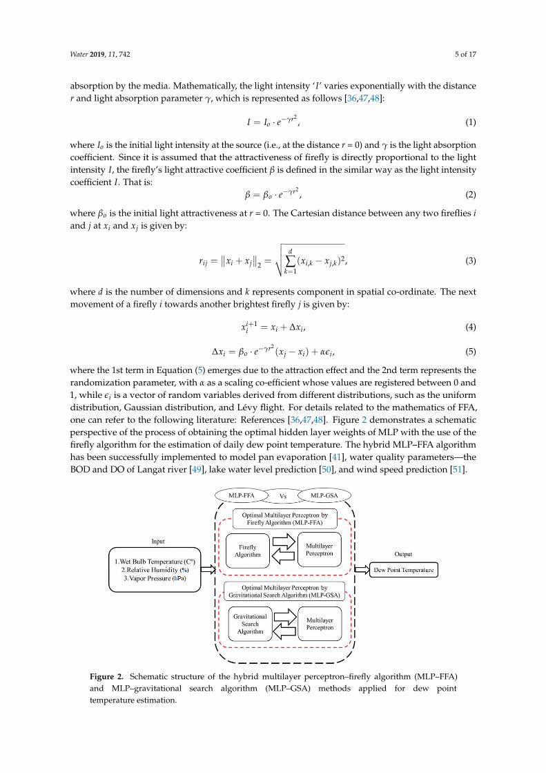
where the 1st term in Equation (5) emerges due to the attraction effect and the 2nd term represents therandomization parameter, with α as a scaling co-efficient whose values are registered between 0 and1, while εi is a vector of random variables derived from different distributions, such as the uniformdistribution, Gaussian distribution, and Lévy flight. For details related to the mathematics of FFA,one can refer to the following literature: References [36,47,48]. Figure 2 demonstrates a schematicperspective of the process of obtaining the optimal hidden layer weights of MLP with the use of thefirefly algorithm for the estimation of daily dew point temperature. The hybrid MLP–FFA algorithmhas been successfully implemented to model pan evaporation [41], water quality parameters—theBOD and DO of Langat river [49], lake water level prediction [50], and wind speed prediction [51].

Figure 2. Schematic structure of the hybrid multilayer perceptron–firefly algorithm (MLP–FFA)and MLP–gravitational search algorithm (MLP–GSA) methods applied for dew pointtemperature estimation.

Water 2019, 11, 742 6 of 17

2.3. Hybridized MLP–GSA Model

The gravitational dearch algorithm (GSA) was introduced by Reference [35]. GSA is based onthe concept of the population search of the Newtonian gravity principle. In the present study, GSAis used for arriving at optimal weights and biases of the MLP network which satisfy the minimumerror criteria. Initially, to evaluate an agent’s fitness, preferably any error criteria of the fitness function,such as MSE, should be defined along with a strategy to encode the optimal weights and biases ofthe MLP network [52]. The positions of ‘agents’, also referred to as ‘objects’, are the solutions in theGSA population and the fitness function is determined by the gravitational and inertial masses of theagents. Due to gravitational force, all the lighter objects are attracted towards the object with heaviermass in proportion to their distances, thus representing a global movement (exploration step) of theobjects. The slow movement of heavier objects (good solutions) guarantees the exploitation step ofthe GSA algorithm. The optimization process of GSA starts with the positioning of agents randomlywith random velocity values and initialization of the gravitational constant. Consequently, the fitnessof each agent according to the defined objective function is evaluated, and the gravitational constant,G(t), is updated. At a specific time t, the force acting on object ‘i′ due to the movement of object ‘j′ isdefined by:

Fdij(t) = G(t)

Mpi(t)×Maj(t)Rij(t) + ε

(xd

j (t)− xdi (t)

), (6)

where Maj is the active gravitational mass related to agent ‘j′ and Mpi is the passive gravitational massrelated to agent ‘i′. The gravitational constant G(t) and the Euclidian distance Rij(t) between twoagents ‘i′ and ‘j′ are calculated as follows:

G(t) = Go · exp(−α× itermaxiter

), (7)

Rij(t) =∥∥Xi(t), Xj(t)

∥∥2 , (8)

where α is the descending coefficient, Go is the initial gravitational constant, ‘iter′ is the current iteration,and ‘maxiter′ is the maximum number of iterations. In a ‘d′ dimensional problem space, the total forcethat acts on agent ‘i′ is given by:

Fdi (t) =

N

∑j=1,j 6=1

randjFdij(t), (9)

where randj is a random number in the interval [0, 1]. Based on the law of motion, the acceleration ofall agents at time ‘t′, and in dth direction is calculated as follows:

adi (t) =

Fdi (t)

Mii(t), (10)

where Mii is the inertial mass of ith agent. Furthermore, the searching strategy of an agent is dependenton the velocity and position of agents which are calculated as follows:

vdi (t + 1) = randi × vd

i (t) + adi (t), (11)

xdi (t + 1) = xd

i (t) + vdi (t + 1). (12)

The updating process is repeated as long as the stopping criterion is not satisfied. When a certainstopping criterion is met, or soon after the maximum number of iterations are reached, the GSAalgorithm ceases. The superiority of GSA is due to two steps: Exploration (potential to navigate in thespace) and exploitation (potential to search optima around the best solution). For additional detailsrelated to GSA, one may refer to Xing and Gao (2014) [53] and Jadidi et al. (2013) [54]. The schematicstructure of the MLP–GSA is shown in Figure 2.

Water 2019, 11, 742 7 of 17

3. Study Area and Data Description

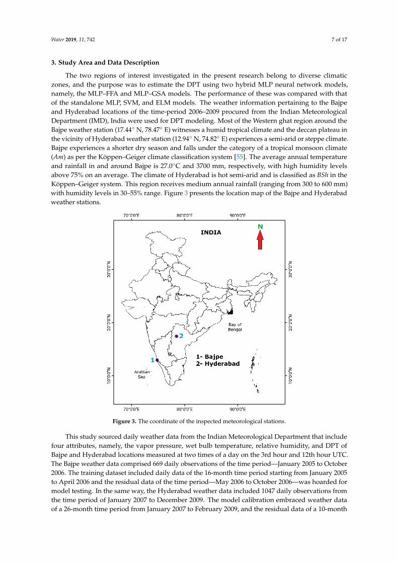
The two regions of interest investigated in the present research belong to diverse climaticzones, and the purpose was to estimate the DPT using two hybrid MLP neural network models,namely, the MLP–FFA and MLP–GSA models. The performance of these was compared with thatof the standalone MLP, SVM, and ELM models. The weather information pertaining to the Bajpeand Hyderabad locations of the time-period 2006–2009 procured from the Indian MeteorologicalDepartment (IMD), India were used for DPT modeling. Most of the Western ghat region around theBajpe weather station (17.44◦ N, 78.47◦ E) witnesses a humid tropical climate and the deccan plateau inthe vicinity of Hyderabad weather station (12.94◦ N, 74.82◦ E) experiences a semi-arid or steppe climate.Bajpe experiences a shorter dry season and falls under the category of a tropical monsoon climate(Am) as per the Köppen–Geiger climate classification system [55]. The average annual temperatureand rainfall in and around Bajpe is 27.0◦C and 3700 mm, respectively, with high humidity levelsabove 75% on an average. The climate of Hyderabad is hot semi-arid and is classified as BSh in theKöppen–Geiger system. This region receives medium annual rainfall (ranging from 300 to 600 mm)with humidity levels in 30–55% range. Figure 3 presents the location map of the Bajpe and Hyderabadweather stations.

Figure 3. The coordinate of the inspected meteorological stations.

This study sourced daily weather data from the Indian Meteorological Department that includefour attributes, namely, the vapor pressure, wet bulb temperature, relative humidity, and DPT ofBajpe and Hyderabad locations measured at two times of a day on the 3rd hour and 12th hour UTC.The Bajpe weather data comprised 669 daily observations of the time period—January 2005 to October2006. The training dataset included daily data of the 16-month time period starting from January 2005to April 2006 and the residual data of the time period—May 2006 to October 2006—was hoarded formodel testing. In the same way, the Hyderabad weather data included 1047 daily observations fromthe time period of January 2007 to December 2009. The model calibration embraced weather dataof a 26-month time period from January 2007 to February 2009, and the residual data of a 10-month

Water 2019, 11, 742 8 of 17

time period from March 2009 to December 2009 were hoarded for testing of the developed models.The most influential weather parameters that supplement as inputs for DPT estimation were foundby cross-correlation analysis. The vapor pressure, wet bulb temperature, and relative humidity werefound to have good correlation with DPT (refer to Table 1) and were hence considered as inputattributes. Table 2 presents the statistical parameters such as mean, maximum (Max), minimum (Min),standard deviation (S.Dev.), skewness (Skew), and variance (Var.) of weather parameters employed inthe study.

Table 1. Correlation coefficient statistic of DPT with other model input attributes.

CorrelationCo-Efficient

Bajpe Station Hyderabad Station

3rd Hour UTC 12th Hour UTC 3rd Hour UTC 12th Hour UTC

DPT (◦C) DPT (◦C) DPT (◦C) DPT (◦C)

WBT (◦C) 0.97 0.9 0.9 0.87RH (%) 0.75 0.8 0.69 0.83

VP (hPa) 0.99 0.99 0.98 0.99DPT (◦C) 1 1 1 1

Table 2. Statistical parameters of the dataset.

TRAIN TEST

WBT (◦C) RH (%) VP (hPa) DPT (◦C) WBT (◦C) RH (%) VP (hPa) DPT (◦C)

3rd Hour UTC

BajpeStation

Min 15.6 39 11.7 9.3 22.6 73 25.3 22.1Max 24.4 78 27.9 22.9 24.8 84 29.3 23.7

Mean 23.1 77 25.95 21.65 24.6 82.5 29.1 23.6S.Dev. 1.83 1.41 2.75 1.76 0.28 2.12 0.28 0.14

Var. 3.38 2 7.6 3.12 0.08 4.5 0.08 0.02Skew. −0.97 −0.83 −1.04 −1.46 1.17 0.72 0.18 0.19

12th Hour UTC

Min 19.8 27 13.3 11.2 25 65 27.6 22.7Max 24.8 66 27.1 22.4 25.8 82 31.3 24.8

Mean 24.3 65 26.35 21.95 25.4 73.5 29.45 23.75S.Dev 0.7 1.41 1.06 0.63 0.56 12.02 2.61 1.48Var. 0.5 2 1.125 0.4 0.32 144.5 6.845 2.205

Skew. −0.72 0.1 −0.86 −1.27 −0.57 −0.14 −0.18 −0.31

HyderabadStation

3rd Hour UTC

Min 10.6 26 7.7 3.3 17.2 29 11.3 8.8Max 19 73 16.5 14.5 19 86 20.8 18.1

Mean 17.7 59 16.3 14.3 18.1 57.5 16.05 13.45S.Dev. 1.83 19.79 0.28 0.28 1.27 40.3 6.71 6.57

Var. 3.38 392 0.08 0.08 1.62 162.5 45.12 43.24Skew. −0.57 −0.35 −0.34 −0.75 −0.93 −0.3 −0.69 −1.14

12th Hour UTC

Min 17.8 25 13.9 11.9 20.4 23 13.1 11Max 21.4 40 14.8 12.8 20.6 55 19.6 17.2

Mean 19.6 32.5 14.35 12.35 20.5 39 16.35 14.1S.Dev. 2.54 10.6 0.63 0.63 0.14 22.62 4.59 4.38

Var. 6.48 112.5 0.405 0.405 0.02 512 21.12 19.22Skew −0.32 0.63 0.19 −0.19 −0.71 0.41 −0.26 −0.65

4. Model Development and Performance Analysis

The input/output (I/O) structure formulated for the development of MLP–FFA, MLP–GSA,and the standalone AI models were based on the correlated weather information with the target

Water 2019, 11, 742 9 of 17

variable—DPT (Table 1). The DPT models of the 3rd hour and 12th hour UTC were calibratedindividually using the I/O structure as mentioned below.

Dew Point Temperature (DPT)→ f [WBT + RH + VP] (13)

MLP training refers to a search process for identification of an optimized set of weight andbias values, which can minimize the mean squared error (MSE) across the estimated and real datain the output layer. As already mentioned, a standalone MLP network was trained using an LMback-propagation algorithm. A structured trial and error method was used to find the optimal numberof hidden layer neurons, values of the learning rate, and momentum terms in accordance to theminimum MSE criteria. The FFA and GSA parameters used while training the hybrid MLP modelsare mentioned in Table 3. The learning rate (which controls weight and bias change in each iteration)and the number of hidden neurons of MLP were optimized using the FFA and GSA algorithms.The proposed hybrid ML models were developed using Matlab software.

Performance evaluation: The statistical evaluation measures are endowed with confidence thatcould be relayed on any model estimates. In the present case, the error and efficiency measures such asRMSE, MAE, and NSE were employed to assess the model performance.

Root mean square error (RMSE):

RMSE =

√∑n

i=1(xi − yi)2

n(14)

Mean absolute error (MAE):

MAE =∑n

i=1 |yi − xi|n

(15)

Nash Sutcliffe efficiency (NSE):

NSE = 1− ∑ni=1(yi − xi)

2

∑ni=1(xi − x)2 (16)

where xi—the actual observation; yi—the predicted value; x—mean observation; n—number ofexamined dataset.

Table 3. Parameter settings of FFA and GSA.

MLP–FFA MLP–GSA

Maximum iterations = 180 Maximum iterations = 180Population size: 50 Population size: 50βo = 0.9 Acceleration Co-efficients (α, β) = 1γ = 1 ω (weighting function) = [0.4, 0.9]εi = 0.97 Initial velocities of agents are randomly

generated in the interval [0,1]α = 0.6

5. Results and Discussion

Without any doubt, there exist several soft computing models that have shown excellentperformance in modeling dew point temperature [24,28]. However, researchers have been extremelyzealous to navigate through new methodologies for the sake of attaining more reliable and robustmodels for solving any kind of complex nonlinear problems. The current research demonstrated thehybridization of the classical artificial intelligence model with nature-inspired optimization algorithmsfor impersonating the actual physic concept—DPT. The performance of hybrid models (i.e., MLP–FFAand MLP–GSA) in estimating daily DPT were evaluated against SVM and ELM model results reportedin Deka et al. (2018) [26], since the models developed in this study used the same data and model

Water 2019, 11, 742 10 of 17

(input–output) structure of the earlier research by Deka et al. (2018) [26]. Tables 4 and 5 presentthe performance of hybrid MLP networks (MLP–FFA and MLP–GSA) and other models (MLP, SVM,and ELM), evaluated in terms of various performance statistics along with relevant model parametersor network configurations. The input variables (wet bulb temperature (WBT), relative humidity(RH), and vapor pressure (VP)) derived from the cross-correlation analyses in conjunction with thedependent variable (DPT) were appropriate for model development and therefore resulted in goodefficiency measures.

Table 4. The performance of the computed metrics for Bajpe station.

MODEL Model Parameters/Structure Testing

RMSE (◦C) MAE (◦C) NSE

3rd hourUTC

SVM * 28,8,0.01 0.480 0.210 0.520ELM * 3-40-1 0.380 0.040 0.690MLP (3,16,1) 0.051 0.016 0.995MLP–FFA (3,16,1) 0.034 0.011 0.998MLP–GSA (3,16,1) 0.041 0.013 0.997

12th hourUTC

SVM * 28,7,0.01 0.520 0.28 0.62ELM * 3-90-1 0.100 0.02 0.9MLP (3,13,1) 0.039 0.016 0.998MLP–FFA (3,13,1) 0.026 0.010 0.999MLP–GSA (3,13,1) 0.031 0.013 0.999

Note: Model Parameters of SVM—(C, γ, ε);ELM—(input–hidden–output layer neurons);MLP—(input, hidden, output layer neurons)

* Deka et al. (2018) [26].

Table 5. The performance of the computed metrics for Hyderabad station.

MODEL Model Parameters/Structure Testing

RMSE (◦C) MAE (◦C) NSE

3rd hourUTC

SVM * 37,12,0.01 2.360 1.040 0.630ELM * 3-50-1 0.630 0.320 0.950MLP (3,4,1) 0.104 0.051 0.999MLP–FFA (3,4,1) 0.069 0.034 0.999MLP–GSA (3,4,1) 0.083 0.041 0.999

12th hourUTC

SVM * 41,14,0.01 1.980 1.050 0.820ELM * 3-70-1 0.590 0.140 0.970MLP (3,19,1) 0.134 0.052 0.999MLP–FFA (3,19,1) 0.089 0.034 0.999MLP–GSA (3,19,1) 0.107 0.041 0.999

Note: Model Parameters of SVM—(C, γ, ε);ELM—(input–hidden–output layer neurons);MLP—(input, hidden, output layer neurons)

* Deka et al. (2018) [26].

With reference to Bajpe weather station, the MLP–FFA hybrid model is consistently the superiorone when compared to others in terms of all performance statistics for the estimation of both the 3rd and12th hour UTC DPT (see Table 4). In parallel, the efficiencies of MLP–GSA revealed similar skills in theestimation process. It can be observed that the absolute error measurements indicated the superiorityof the proposed hybrid models over MLP, SVM, and ELM estimates. In quantitative terms, for instance,the MLP–FFA model reported a remarkable enhancement of RMSE/MAE by (33/31%), (91/73%),and (92/95%) over the MLP, SVR, and ELM models, respectively; and likewise, the MLP–GSA modelestimates reported a percentage enhancement by (19/18%), (89/67%), and (91/93%) over the MLP,

Water 2019, 11, 742 11 of 17

SVM, and ELM models, respectively (in the case of the 3rd hour DPT modeling). The hybridization ofnature-inspired algorithms with MLP proved to yield powerful predictive models and can contributeto modeling any kind of environmental processes.

With reference to Hyderabad weather station, the hybrid MLP–FFA and MLP–GSA networks againvalidated superior performance with the same statistical metrics run for the previous one (see Table 5).In this case, what can be noticed remarkably is the NSE values which are very close to unity, indicatinga superior performance by the models. The comparative analysis of model performance measuresreveals that the DPT estimates of standard MLP and its hybrid structures (MLP–FFA and MLP–GSA)have low error estimates (RMSE and MSE) in contrast to the SVM and ELM models. The performanceof the MLP–FFA networks was relatively superior to the MLP–GSA models in terms of computationalspeed and accuracy. The speed of convergence of FFA is very high in probability of finding the globaloptimized solutions because of Gaussian or Lévy flight searches, and sometimes, the FFA is consideredas a generalization to three different approaches, namely, particle swarm optimization (PSO), simulatedannealing (SA), and differential evolution (DE) [48]. It is evident that= the integration of GSA withMLP also provides good estimates of DPT, and the gravitational constant and acceleration of particlesare the parameters that are crucial in regulating the exploratory capabilities of the GSA algorithm [56].

An excellent way of graphical presentation was considered for the prediction skill illustrationthrough Taylor diagrams (see Figures 4 and 5), for both the 3rd and 12th hour UTC DPT models.The Taylor diagram provides a concise statistical summary of modeled data in terms of its standarddeviation, root mean square difference and the correlation with actual data [57]. It shows how well thepredictive models match the actual records of DPT of the testing phase with regard to both investigatedclimate zones. The relative merits of models developed can be assessed from high correlation andlow RMS errors represented by points nearest to the reference point (i.e., the actual data). The resultstatistics of the MLP–FFA and MLP–GSA models were closer to the observation point, reaffirmingthe better accuracy of the hybridized models over its comparison counterparts. On comparing thepoint–density plots, presented in Figures 6 and 7, no significant differences were evident amongthe pair of observed vs. (MLP–FFA and MLP–GSA) model estimates with respect to the extreme(minimum and maximum) values and any outliers. It is also evident that the spreads of observed vs.(SVM and ELM) modeled DPTs fluctuate and were dissimilar to each other, assuring variations in theoverall pattern of the estimated time-series data.

Figure 4. Taylor diagram for performance evaluation of the models with respect to Bajpe station.

Water 2019, 11, 742 12 of 17

Figure 5. Taylor diagram for performance evaluation of the models with respect to Hyderabad station.

Figure 6. Point density plots of observed vs. estimated DPTs with respect to Bajpe station.

Water 2019, 11, 742 13 of 17

Figure 7. Point density plots of observed vs. estimated DPTs with respect to Hyderabad station.

Taking into account the disadvantages of the back-propagation (BP) algorithm as discussed inthe earlier part of the manuscript, the novel methods of network adaptation were tested via the FFAand GSA algorithms, by implementing the phase of nonrandom initialization of weight vector ‘w’.It is nothing unexpected that the MLP network integrated with FFA or GSA for weights adjustmentgave altogether better results than the standard MLP. Moreover, in addition to lower RMSE and MAE,another advantage of hybridizing MLP with FFA or GSA is the consistency of estimates. The NSEsof the MLP–FFA and MLP–GSA networks are remarkably higher than those of the SVM and ELMmodels. The acceptable level of accuracy attained using the proposed methodology evidenced thepotential of the hybrid intelligent models for DPT estimation where it is highly essential for practicalimplementation, and especially in the case of designing an online estimation system for monitoringthe DPT fluctuation and using that accurate information for water engineering management and itsrelated applications.

It is worth reporting here, since the main focus of the current research was on the development andapplication of hybrid MLP models for dew point temperature estimation, the uncertainty estimationand analysis using statistical methods would be one of the possible future focuses of research. As amatter of fact, the uncertainties are incorporated in different forms, such as data uncertainty, modeling

Water 2019, 11, 742 14 of 17

uncertainty, and input variability uncertainty. Hence, investigating those types of uncertainties ishighly essential for modeling predictability evaluation.

6. Conclusions

Dew point temperature estimation is of great interest to agro–climatologists for several studies thatneed continuous DPT data. The missing DPT data records could be in-filled using several estimationtechniques. In recent times, time-series based machine learning algorithms have been advantageousover conventional physics-based approaches in terms of solving complex regression problems withless computational cost. This study was intended to explore new hybrid intelligent predictive modelsto estimate DPTs of humid and semi-arid regions of India. The hybrid MLP–FFA and MLP–GSAnetworks were trained to estimate the daily DPTs using correlated weather variables, including WBT,RH, and VP, as inputs. MLP–FFA obtained the best results with significantly faster convergenceability. The three evaluation indices gave definitely no reason to discard the superiority of MLP and itshybrid structures over the SVM and ELM models. The efficiency of the MLP network is dependent onthe optimal tuning for the input parameters in addition to architecture type and training algorithmemployed. The nature-inspired optimization algorithms certainly augment the predictability of theclassical MLP model. The performance of both the MLP–FFA and MLP–GSA networks exhibited anacceptable level of accuracy and enhancement for both inspected climactic zones. However, MLP–FFAemerged as the most optimal technique compared to others in terms of the minimum error criteria.

Author Contributions: Conceptualization, S.R.N.; Data analysis, S.R.N.; Formal analysis, S.M.B.;Funding acquisition, N.A.-A.; Investigation, S.M.B.; Methodology, M.A.G.; Project administration, S.M.B.;Software, S.R.N. and M.A.G.; Supervision, P.C.D.; Validation, Z.M.Y.; Visualization, Z.M.Y.; Writing—originaldraft, S.R.N.; Writing—review and editing, Z.M.Y., P.C.D., and N.A.-A.

Funding: This research received no external funding.

Acknowledgments: The scholars of the present work would like to reveal their gratitude and appreciation to thedata provider, the Indian Meteorological Department, Ministry of Earth Sciences, Govt. of India.

Conflicts of Interest: The authors declare no conflict of interest.

References

1. Wood, L.A. The use of dew-point temperature in humidity calculations. J. Res. Notional Bur. Stand. 1970, 74,117–122. [CrossRef]

2. Ben-Asher, J.; Alpert, P.; Ben-Zvi, A. Dew is a major factor affecting vegetation water use efficiency ratherthan a source of water in the eastern Mediterranean area. Water Resour. Res. 2010, 46, W10532. [CrossRef]

3. Ahrens, C.D. Meteorology Today; Chapter Condensation: Dew, Fog, and Clouds; Thomson Higher Education:Belmont, CA, USA, 2007; pp. 106–137.

4. Changnon, D.; Sandstrom, M.; Schaffer, C. Relating changes in agricultural practices to increasing Dewpoints in extreme Chicago heat waves. Clim. Res. 2003, 24, 243–254. [CrossRef]

5. McHugh, T.A.; Morrissey, E.M.; Reed, S.C.; Hungate, B.A.; Schwartz, E. Water from air: An overlookedsource of moisture in arid and semiarid regions. Sci. Rep. 2015, 5, 13767. [CrossRef] [PubMed]

6. Agam, N.; Berliner, P. Dew formation and water vapor adsorption in semi-arid environments—A review.J. Arid Environ. 2006, 65, 572–590.

7. Eccel, E. Estimating air humidity from temperature and precipitation measures for modelling applications.Meteorol. Appl. 2012, 19, 118–128. [CrossRef]

8. Ebrahimpour, M.; Ghahreman, N.; Orang, M. Assessment of climate change impacts on referenceevapotranspiration and simulation of daily weather data using SIMETAW. J. Irrig. Drain. Eng. 2014,140, 04013012. [CrossRef]

9. Mahmood, R.; Hubbard, K.G. Assessing bias in evapotranspiration and soil moisture estimates due to theuse of modeled solar radiation and dew point temperature data. Agric. For. Meteorol. 2005, 130, 71–84.[CrossRef]

Water 2019, 11, 742 15 of 17

10. McMahon, T.; Peel, M.; Lowe, L.; Srikanthan, R.; McVicar, T. Estimating actual, potential, reference cropand pan evaporation using standard meteorological data: A pragmatic synthesis. Hydrol. Earth Syst. Sci.2013, 17, 1331–1363. [CrossRef]

11. Roberts, J.S. Encyclopedia of Agricultural, Food and Biological Engineering; Chapter Dew Point Temperature;CRC Press: Boca Raton, FL, USA, 2003; pp. 186–191.

12. Lawrence, M.G. The relationship between relative humidity and the Dewpoint temperature in moist air:A simple conversion and applications. Bull. Am. Meteorol. Soc. 2005, 86, 225–233.

13. Pokhrel, P.; Wang, Q.; Robertson, D.E. The value of model averaging and dynamical climate modelpredictions for improving statistical seasonal streamflow forecasts over Australia. Water Resour. Res. 2013, 49,6671–6687. [CrossRef]

14. Liu, Z.; Zhou, P.; Chen, X.; Guan, Y. A multivariate conditional model for streamflow prediction and spatialprecipitation refinement. J. Geophys. Res. Atmos. 2015, 120. [CrossRef]

15. Liu, Z.; Cheng, L.; Hao, Z.; Li, J.; Thorstensen, A.; Gao, H. A framework for exploring joint effects ofconditional factors on compound floods. Water Resour. Res. 2018, 54, 2681–2696. [CrossRef]

16. Khedun, C.P.; Mishra, A.K.; Singh, V.P.; Giardino, J.R. A copula-based precipitation forecasting model:Investigating the interdecadal modulation of ENSO’s impacts on monthly precipitation. Water Resour. Res.2014, 50, 580–600. [CrossRef]

17. Tao, H.; Diop, L.; Bodian, A.; Djaman, K.; Ndiaye, P.M.; Yaseen, Z.M. Reference evapotranspiration predictionusing hybridized fuzzy model with firefly algorithm: Regional case study in Burkina Faso. Agric. Water Manag.2018, 208, 140–151. [CrossRef]

18. Shank, D.B.; McClendon, R.W.; Paz, J.; Hoogenboom, G. Ensemble Artificial Neural Networks for predictionof Dew point temperature. Appl. Artif. Intell. 2008, 22, 523–542. [CrossRef]

19. Zounemat-Kermani, M. Hourly predictive Levenberg–Marquardt ANN and multi linear regression modelsfor predicting of Dew point temperature. Meteorol. Atmos. Phys. 2012, 117, 181–192. [CrossRef]

20. Nadig, K.; Potter, W.; Hoogenboom, G.; McClendon, R. Comparison of individual and combined ANNmodels for prediction of air and Dew point temperature. Appl. Intell. 2013, 39, 354–366. [CrossRef]

21. Kisi, O.; Kim, S.; Shiri, J. Estimation of Dew point temperature using Neuro-fuzzy and Neural networktechniques. Theor. Appl. Climatol. 2013, 114, 365–373. [CrossRef]

22. Shiri, J.; Kim, S.; Kisi, O. Estimation of daily Dew point temperature using Genetic Programming and NeuralNetworks approaches. Hydrol. Res. 2014, 45, 165–181. [CrossRef]

23. Kim, S.; Singh, V.P.; Lee, C.J.; Seo, Y. Modeling the physical dynamics of daily Dew point temperature usingsoft computing techniques. KSCE J. Civ. Eng. 2015, 19, 1930–1940. [CrossRef]

24. Mohammadi, K.; Shamshirband, S.; Motamedi, S.; Petkovic, D.; Hashim, R.; Gocic, M. Extreme learningmachine based prediction of daily Dew point temperature. Comput. Electron. Agric. 2015, 117, 214–225.[CrossRef]

25. Mohammadi, K.; Shamshirband, S.; Petkovic, D.; Yee, L.; Mansor, Z. Using ANFIS for selection of morerelevant parameters to predict Dew point temperature. Appl. Therm. Eng. 2016, 96, 311–319. [CrossRef]

26. Deka, P.C.; Patil, A.P.; Yeswanth Kumar, P.; Naganna, S.R. Estimation of dew point temperature using SVMand ELM for humid and semi-arid regions of India. ISH J. Hydraul. Eng. 2018, 24, 190–197. [CrossRef]

27. Attar, N.F.; Khalili, K.; Behmanesh, J.; Khanmohammadi, N. On the reliability of soft computing methods inthe estimation of dew point temperature: The case of arid regions of Iran. Comput. Electron. Agric. 2018, 153,334–346. [CrossRef]

28. Baghban, A.; Bahadori, M.; Rozyn, J.; Lee, M.; Abbas, A.; Bahadori, A.; Rahimali, A. Estimation of airDew point temperature using computational intelligence schemes. Appl. Therm. Eng. 2016, 93, 1043–1052.[CrossRef]

29. Al-Shammari, E.T.; Mohammadi, K.; Keivani, A.; Ab Hamid, S.H.; Akib, S.; Shamshirband, S.; Petkovic, D.Prediction of daily dewpoint temperature using a model combining the support vector machine with fireflyalgorithm. J. Irrig. Drain. Eng. 2016, 142, 04016013. [CrossRef]

30. Amirmojahedi, M.; Mohammadi, K.; Shamshirband, S.; Danesh, A.S.; Mostafaeipour, A.; Kamsin, A.A hybrid computational intelligence method for predicting dew point temperature. Environ. Earth Sci.2016, 75, 415. [CrossRef]

31. Ludermir, T.B.; Yamazaki, A.; Zanchettin, C. An optimization methodology for neural network weights andarchitectures. IEEE Trans. Neural Networks 2006, 17, 1452–1459. [CrossRef]

Water 2019, 11, 742 16 of 17

32. Lawrence, S.; Giles, C.L.; Tsoi, A.C. What Size Neural Network Gives Optimal Generalization?Convergence Properties of Backpropagation; Technical Report CS-TR-3617; University of Maryland, CollegePark, MD, USA, 1996.

33. Lawrence, S.; Giles, C.L. Overfitting and neural networks: Conjugate gradient and backpropagation.In Proceedings of the IEEE-INNS-ENNS International Joint Conference on Neural Networks, Como, Italy,27 July 2000; Volume 1, pp. 114–119.

34. Nayak, J.; Naik, B.; Behera, H. A novel nature inspired firefly algorithm with higher order neural network:Performance analysis. Eng. Sci. Technol. Int. J. 2016, 19, 197–211. [CrossRef]

35. Rashedi, E.; Nezamabadi-pour, H.; Saryazdi, S. GSA: A Gravitational Search Algorithm. Inf. Sci. 2009, 179,2232–2248. [CrossRef]

36. Yang, X.S. Firefly algorithm, stochastic test functions and design optimisation. Int. J. Bio-Inspired Comput.2010, 2, 78–84. [CrossRef]

37. Siddiquea, N.; Adelib, H. Applications of gravitational search algorithm in engineering. J. Civ. Eng. Manag.2016, 22, 981–990. [CrossRef]

38. Yang, X.S.; He, X. Firefly algorithm: Recent advances and applications. Int. J. Swarm Intell. 2013, 1, 36–50.[CrossRef]

39. Gardner, M.W.; Dorling, S. Artificial Neural Networks (the Multilayer Perceptron)–a review of applicationsin the atmospheric sciences. Atmos. Environ. 1998, 32, 2627–2636. [CrossRef]

40. Fabbian, D.; de Dear, R.; Lellyett, S. Application of artificial neural network forecasts to predict fog atCanberra International Airport. Weather Forecast. 2007, 22, 372–381. [CrossRef]

41. Ghorbani, M.; Deo, R.C.; Yaseen, Z.M.; Kashani, M.H.; Mohammadi, B. Pan evaporation predictionusing a hybrid multilayer perceptron-firefly algorithm (MLP-FFA) model: Case study in North Iran.Theor. Appl. Climatol. 2018, 133, 1119-1131. [CrossRef]

42. Ghorbani, M.A.; Zadeh, H.A.; Isazadeh, M.; Terzi, O. A comparative study of artificial neural network(MLP, RBF) and support vector machine models for river flow prediction. Environ. Earth Sci. 2016, 75, 476.[CrossRef]

43. Rumelhart, D.E.; McClelland, J.L. Parallel Distributed Processing; MIT Press: Cambridge, MA, USA, 1987;Volume 1.

44. Lek, S.; Park, Y. Artificial Neural Networks. In Encyclopedia of Ecology; Academic Press: Oxford, UK, 2008;pp. 237–245.

45. Haykin, S.S. Neural Networks and Learning Machines, 3rd ed.; Prentice-Hall: Upper Saddle River, NJ, USA,2009; p. 906.

46. Park, Y.S.; Lek, S. Artificial Neural Networks: Multilayer Perceptron for Ecological Modeling. In EcologicalModel Types; Developments in Environmental Modelling; Elsevier: Amsterdam, The Netherlands, 2016;Volume 28, pp. 123 – 140.

47. Zhang, L.; Liu, L.; Yang, X.S.; Dai, Y. A Novel Hybrid Firefly Algorithm for Global Optimization. PLoS ONE2016, 11, 1–17. [CrossRef]

48. Iztok, F.; Iztok, F.J.; Xin-She, Y.; Janez, B. A comprehensive review of Firefly algorithms. Swarm Evol. Comput.2013, 13, 34 – 46.

49. Raheli, B.; Aalami, M.T.; El-Shafie, A.; Ghorbani, M.A.; Deo, R.C. Uncertainty assessment of the multilayerperceptron (MLP) neural network model with implementation of the novel hybrid MLP-FFA methodfor prediction of biochemical oxygen demand and dissolved oxygen: A case study of Langat River.Environ. Earth Sci. 2017, 76, 503. [CrossRef]

50. Ghorbani, M.A.; Deo, R.C.; Karimi, V.; Yaseen, Z.M.; Terzi, O. Implementation of a hybrid MLP-FFA modelfor water level prediction of Lake Egirdir, Turkey. Stoch. Environ. Res. Risk Assess. 2017, 32, 1683–1697.[CrossRef]

51. Deo, R.C.; Ghorbani, M.A.; Samadianfard, S.; Maraseni, T.; Bilgili, M.; Biazar, M. Multi-layer perceptronhybrid model integrated with the Firefly optimizer algorithm for windspeed prediction of target site using alimited set of neighboring reference station data. Renew. Energy 2018, 116, 309–323. [CrossRef]

52. Mirjalili, S.; Hashim, S.Z.M.; Sardroudi, H.M. Training Feedforward Neural Networks using hybrid particleswarm optimization and Gravitational Search Algorithm. Appl. Math. Comput. 2012, 218, 11125–11137.[CrossRef]

Water 2019, 11, 742 17 of 17

53. Xing, B.; Gao, W.J. Gravitational Search Algorithm. In Innovative Computational Intelligence: A Rough Guide to134 Clever Algorithms; Springer International Publishing: Berlin, Germany, 2014; pp. 355–364.

54. Jadidi, Z.; Muthukkumarasamy, V.; Sithirasenan, E.; Sheikhan, M. Flow-Based Anomaly Detection UsingNeural Network Optimized with GSA Algorithm. In Proceedings of the 2013 IEEE 33rd InternationalConference on Distributed Computing Systems Workshops, Philadelphia, PA, USA, 8–11 July 2013; pp. 76–81.

55. Peel, M.C.; Finlayson, B.L.; McMahon, T.A. Updated world map of the Köppen-Geiger climate classification.Hydrol. Earth Syst. Sci. 2007, 11, 1633–1644. [CrossRef]

56. de Moura Oliveira, P.B.; Oliveira, J.; Cunha, J.B. Trends in Gravitational Search Algorithm. In 14thInternational Conference on Distributed Computing and Artificial Intelligence; Omatu, S., Rodríguez, S.,Villarrubia, G., Faria, P., Sitek, P., Prieto, J., Eds.; Springer International Publishing: Berlin, Germany,2018; pp. 270–277.

57. Taylor, K.E. Summarizing multiple aspects of model performance in a single diagram. J. Geophys. Res. Atmos.2001, 106, 7183–7192. [CrossRef]

c© 2019 by the authors. Licensee MDPI, Basel, Switzerland. This article is an open accessarticle distributed under the terms and conditions of the Creative Commons Attribution(CC BY) license (http://creativecommons.org/licenses/by/4.0/).