Development of a test procedure for water sensitivity of ...
320
AN ABSTRACT OF THE THESIS OF Saleh H. Al-Swailmi for the degree of Doctor of Philosophy in Civil Engineering presented on May 5. 1992. Title: Development of a Test Procedure for Water Sensitivity of Asphalt Concrete Mixtures Redacted for Privacy Abstract approved: Ronald L. Terrel Environmental factors such as temperature, air, and water can have a profound effect on the durability of asphalt concrete mixtures. In mild climates where good quality aggregates and asphalt cement are available, the major contribution to deterioration may be due to traffic loading and the resultant distress is manifested in the form of fatigue cracking, rutting, and raveling. But, when more severe climates are coupled with poor materials and traffic, premature failure may result. The objectives of this research are twofold and includes: (1) development of a test system to evaluate the most important factors influencing the water sensitivity of asphalt concrete mixtures; and (2) development of laboratory testing procedures that will predict field performance. This research also addresses the hypothesis that much of the water damage in pavements is due to water in the asphalt concrete void system. It is proposed that most of the water problems occur when voids are in the range of about 5% to 12%. Thus, the term "pessimum" voids is used to indicate that range (opposite of optimum). In order to evaluate the hypothesis and the numerous variables, the Environmental Conditioning System (ECS) was designed and fabricated. The ECS consists of three
-
Upload
khangminh22 -
Category
Documents
-
view
0 -
download
0
Transcript of Development of a test procedure for water sensitivity of ...
AN ABSTRACT OF THE THESIS OF
Saleh H. Al-Swailmi for the degree of Doctor of Philosophy in Civil Engineering
presented on May 5. 1992.
Title: Development of a Test Procedure for Water Sensitivity of Asphalt Concrete
Mixtures Redacted for Privacy
Abstract approved:Ronald L. Terrel
Environmental factors such as temperature, air, and water can have a profound
effect on the durability of asphalt concrete mixtures. In mild climates where good
quality aggregates and asphalt cement are available, the major contribution to
deterioration may be due to traffic loading and the resultant distress is manifested
in the form of fatigue cracking, rutting, and raveling. But, when more severe
climates are coupled with poor materials and traffic, premature failure may result.
The objectives of this research are twofold and includes: (1) development ofa test
system to evaluate the most important factors influencing the water sensitivity of
asphalt concrete mixtures; and (2) development of laboratory testing procedures that
will predict field performance. This research also addresses the hypothesis that much
of the water damage in pavements is due to water in the asphalt concrete void
system. It is proposed that most of the water problems occur when voids are in the
range of about 5% to 12%. Thus, the term "pessimum" voids is used to indicate that
range (opposite of optimum).
In order to evaluate the hypothesis and the numerous variables, the Environmental
Conditioning System (ECS) was designed and fabricated. The ECS consists of three
subsystems: (1) fluid conditioning, where the specimen is subjected to predetermined
levels of water, air, or vapor and permeability is measured; (2) an environmental
cabinet that controls the temperature and humidity and encloses the entire load
frame; and (3) the loading system that determines resilient modulus (MR) at various
times during environmental cycling and also provides continuous repeated loading
as needed.
The ECS has been used to evaluate four core materials and also to investigate the
relative importance of mixture variables thought to be significant. Many details
regarding specimen preparation and testing procedures were evaluated during a
"shakedown" of the ECS. As minor variables were resolved, a procedure emerged
which appears to be reasonable and suitable. An experiment design for the four core
mixtures was developed, and the overall experiment design included three ranges of
void ( <5% low; 5-12%, pessimum; > 12% high). Six-hour cycles of wet-hot (60° C)
and wet-freeze (-18 ° C) are the principle conditioning variables, while monitoring
MR at 250 C before and between cycling. A conventional testing procedure
(AASHTO T-283) was also used on the core mixtures to provide a baseline for
comparison.
Results to date show that the ECS is capable of discerning the relative differences
in "performance" such as MR. Three hot cycles and one freeze cycle appear to be
sufficient to determine the projected relative performance when comparing different
aggregates, asphalts, void levels, loading, etc. Based on these results, a water
conditioning procedure has been recommended and also a procedure for water
conditioning specimens prior to testing in fatigue, rutting, and thermal cracking.

Copyright by Saleh Al-Swailmi
May 5, 1992
All Rights Reserved
DEVELOPMENT OF A TEST PROCEDURE FOR WATER SENSITIVITY OF
ASPHALT CONCRETE MIXTURES
by
Saleh H. Al-Swailmi
A THESIS
submitted to
Oregon State University
in partial fulfillment of
the requirements for the
degree of
Doctor of Philosophy
Completed May 5, 1992
Commencement June 1992
Approved:
Redacted for Privacy
Professor of Civil Engineering in charge of major
Redacted for Privacy
Head of Delartment of Civil Engineering
Redacted for Privacy
Dean of GraduatI hool
Date thesis is presented: May 5, 1992
Typed by: Gail Barnes and Saleh

ACKNOWLEDGEMENT
I would like to express my sincere appreciation to my parents, to whom this
dissertation is dedicated. I would also like to thank my wife, my daughter Ruba and
my son Thamir for their patience, sacrifices, and support throughout the duration of
this stage of our lives.
My appreciation is also expressed to my major professor, Dr. Ronald Terrel,
for his valuable direction, guidance, and consultation during the course of this study.
In particular, his friendship and support is greatly acknowledged. I would also like
to thank the other members of my graduate committee, Professors Harold Pritchett,
Gary Hicks, Chris Bell, and the Graduate School representative, Professor Thomas
Plant, for their assistance in developing my academic program.
I also wish to thank Gail Barnes and Andy and Nancy Brickman for their help
and assistance in various aspects, and especially, for their friendship. My colleague
Todd Scholz deserves special mention for his valuable programming abilities and
computer interface skills.
This research was supported by the Strategic Highway Research Program (SHRP).
TABLE OF CONTENTS
Chapter Page
1. Introduction 1
1.1 Background 6Test Procedures and Moisture Sensitivity 6Philosophy of Water Damage Mitigation 9
1.2 Hypothesis for Water Damage Mitigation 10Theory for Water Sensitivity Behavior 14Theories for Adhesion 15Theory of Cohesion 17
1.3 Research Objectives 21
2. Experiment Design 242.1 Variables 252.2 Equipment and Procedures 35
Testing System 36Fluid Conditioning Subsystem 38Environmental Conditioning Subsystem 40Loading Subsystem 42
Test Procedures 422.3 Materials 46
3. Test Results 533.1 AASHTO T-283 533.2 Development of Test Methods 55
Resilient Modulus Test 55Test specimen preparation 59Test equipment and instrumentation 59Effect of L/D ratio on Resilient Modulus 61Effect of strain gage glue type 67Repeatability of ECS-MR and effect of teflon disks 68
Permeability Measurements 73Effect of specimen surface flow on permeability 75Effect of compaction procedureon specimen surface sealing 78
Differential pressure level-permeabilityrelationship 80
Permeability as a measure of specimenvolume change 86
Specimen internal coloring indicator 88Methods of Air Void Calculations 90
TABLE OF CONTENTS (continued)
Chapter Page
3.3 Environmental Conditioning System (ECS) 94ECS-MR 99Permeability 102Visual Evaluation 105
4. Discussion and Analysis of Test Results 1084.1 Effect of Mixture Variables 109
Aggregate type 109Asphalt type 114Air void level 118
4.2 Effect of Conditioning Variables 122Conditioning fluid 125Conditioning temperature 127Vacuum level 129Repeated loading 135Conditioning time 142
4.3 Visual Evaluation 1504.4 Permeability 1574.5 Confirmation of Hypothesis 1644.6 Repeatability of ECS 171
Test System Repeatability 172Repeatability of Water Conditioning Procedure 175
4.7 Water Conditioning Procedure 1844.8 AASHTO T-283: Resistance of Compacted Bituminous
Mixtures to Moisture-Induced Damage 192
5. Conclusions 202
6. Recommendations 2066.1 Implementation 206
Testing Equipment 206Water Conditioning Techniques 209
Water conditioning procedure 209Wet conditioning procedure 212
6.2 Future Research 213
7. References 214
TABLE OF CONTENTS (continued)
Chapter Page
8. AppendicesA. Original Test Results of ECS 219B. Standard Method of Test for Determining Moisture Sensitivity
Characteristics of Compacted Bituminous Subjected to Hot andCold Climate Conditions 228
C. Wet Conditioning Protocol 242D. Sample Preparation Protocol 250E. Resistance of Compacted Bituminous Mixture to Moisture
Induced Damage 253F. Permeability Protocol 288G. Standard Test Method for Dynamic Modulus of
Asphalt Mixtures ( ASTM D 3497) 295
LIST OF FIGURES
Figure 1.1 The Relative Strength of Mixtures May Dependon the Access to Water in the Void System
Page
11
Figure 1.2 Mechanisms of Adhesion Improvement With MicrowaveEnergy Treatment (Al-Ohaly and Terrel, 1989) 18
Figure 1.3 The Resilient Modulus of Asphalt Concrete is Sensitive toChanges in Moisture Conditioning (Schmidt and Graf, 1972) 20
Figure 1.4 Possible Improved Test Procedure for Water Sensitivity(Terrel and Shute, 1989) 22
Figure 2.1 Experimental Test Plan and Specimen Identification 28
Figure 2.2 Degree of Saturation- Air Voids Relationship 32
Figure 2.3 Overview of Environmental Conditioning System (ECS) 37
Figure 2.4 Schematic Drawing of Environmental ConditioningSystem (ECS) 39
Figure 2.5 Example of Controlled Environment in the ECS Cabinet 41
Figure 2.6 Load Frame Inside Environmental Cabinet 43
Figure 2.7 Typical Conditioning Information Chart 44
Figure 2.8 Aggregate Gradation 49
Figure 3.1 Overview of the Test Setup 62
Figure 3.2 Relationship Between Resilient Modulus and SpecimenThickness for Two Testing Conditions (Specimen no. 1) 63
Figure 3.3 Relationship Between Resilient Modulus and SpecimenThickness for Two Testing Conditions (Specimen no. 2) 64
Figure 3.4 Relationship Between Resilient Modulus and SpecimenThickness for Two Testing Conditions (Specimen no. 3) 65
Figure 3.5 Effect of Strain Gage Mounting Glue on Resilient Modulus 69
Figure 3.6 Variability of ECS-MR for Different Test Conditions 72
LIST OF FIGURES (continued)Page
Figure 3.7 Water Conditioning Setup for Cylindrical Specimen 74
Figure 3.8 Effect of Different Methods of Specimen Sealing onPermeability 77
Figure 3.9 Schematic Diagram of Permeability Apparatus 82
Figure 3.10 Air Flow Versus Differential Pressurefor Open-Graded Specimen 85
Figure 3.11 The relationship Between SpecimenThickness & Volume Change 89
Figure 3.12 Schematic Diagram of Dye-Treatment Setup 91
Figure 3.13 Comparison of Percent Air Void Calculation Withand Without Parafilm 92
Figure 3.14 Summary of Plots of Different Conditioning Levels 95
Figure 3.15 Schematic Drawing of Vapor Conditioning Setup 101
Figure 3.16 Visual Evaluation Rating Pattern (Field and Phang, 1986) 106
Figure 4.1 Effect of Aggregate/Asphalt Type on Resilient ModulusChange, After Hot-Wet Conditioning 110
Figure 4.2 Effect of Aggregate/Asphalt Type on Resilient ModulusChange, After Freeze-Wet Conditioning 112
Figure 4.3 Effect of Air Voids Level on Resilient Modulus Change 121
Figure 4.4 Effect of Conditioning Fluid on Resilient Modulus Change 126
Figure 4.5 Effect of Conditioning Temperature on ResilientModulus Change 128
Figure 4.6 Effect of Vacuum Level on Resilient Modulus Change, AfterFreeze-Wet Conditioning 133
Figure 4.7 Effect of Vacuum Level on Resilient Modulus Change, AfterHot-Wet Conditioning 134
LIST OF FIGURES (continued)
Page
Figure 4.8 Effect of Hot Wet Conditioning and RepeatedLoading on Permanent Deformation 141
Figure 4.9 Effect of Continuous Repeated Loading on ResilientModulus Change 143
Figure 4.10 Effect of Conditioning Time on Resilient Modulus Change 145
Figure 4.11 Stripping Rate Standards (Calibrated by trial and errorof water Conditioning) 151
Figure 4.12 Effect of Conditioning Factors on Stripping Rate 154
Figure 4.13 Effect of Conditioning Factors on Resilient Modulus Change 156
Figure 4.14 Permeability-Air Voids Relationship 158
Figure 4.15 Permeability-Temperature Relationship 160
Figure 4.16 Effect of Conditioning Factors on Permeability Change 162
Figure 4.17 Resilient Modulus Change After Free DrainageWater Conditioning 169
Figure 4.18 Resilient Modulus Change-Air Void Content RelationshipAfter Free Drainage Water Conditioning 170
Figure 4.19 Repeatability of ECS-MR Test 174
Figure 4.20 Repeatability of Water Conditioning Procedure 179
Figure 4.21 Conditioning Information Charts for ClimateSequence Investigation 186
Figure 4.22 Effect of Conditioning Sequence on ResilientModulus Change, (Freeze-Hot or Hot-Freeze) 188
Figure 4.23 Conditioning Information Charts for Water ConditioningProcedure Investigation 189
Figure 4.24 Effect of Number of Hot Cycles on ResilientModulus Change 191
LIST OF FIGURES (continued)
Page
Figure 4.25 Resilient Modulus Change After AASHTO T 283 Test 194
Figure 4.26 Retained Tensile Strength After AASHTO T 283 Test 195
Figure 6.1 Recommendation Chart as Accomplished in thisWater Sensitivity Study 207
Figure 6.2 Conditioning Charts for Hot and Cold Climates 210
LIST OF TABLESPage
Table 1.1 Factors Influencing Response of Mixtures to Water Sensitivity( Terrel and Shute, 1989) 4
Table 2.1 Considered Factors in The Experiment Plan 27
Table 2.2 Mix Design Results and Compaction Efforts 47
Table 2.3 RL and RB Aggregate Gradation used inthis study (from MRL data) 48
Table 2.4 Physical Properties of Asphalt Materials(from MRL data) 51
Table 2.5 Aggregate Properties (from MRL data) 52
Table 3.1 Typical Data Calculations of AASHTO T-284 Test Results 54
Table 3.2 Summary Table of AASHTO T-283 Test Results 56
Table 3.3 Density and Air Void Calculations for theThree Specimen Thicknesses 60
Table 3.4 Resilient Modulus (ECS-MR) for DifferentTest Conditions 71
Table 3.5 Summary of Permeability Measurements Comparingas-molded Briquets With 1/4" Sawed of Each End 79
Table 3.6 Rate of Air Flow Versus Differential Pressure forOpen-graded Asphalt Concrete Specimen 83
Table 3.7 The Relationship Between r-squared and Permeability 87
Table 3.8 Summary of The ECS Water Conditioning Test Results 96
Table 3.9 Permeability Versus Percent Air Voids 103
Table 4.1 Analysis of Variance of the Difference Between MR RatiosAfter Three Hot-Wet Conditioning Cycles for the FourAsphalt-Aggregate Combinations 113
Table 4.2 Asphalt/Aggregate Ranking by LSD 115
LIST OF TABLES (continued)
Table 4.3 Analysis of Variance of the Difference Between MR RatiosAfter Three Hot-Wet Conditioning Cycles for RB/AAG-1Versus RB/AAK-1 Combination
Page
117
Table 4.4 Analysis of Variance of the Difference Between MR RatiosAfter Three Freeze-Wet Conditioning Cycles for the FourAsphalt-Aggregate Combinations 119
Table 4.5 Asphalt/Aggregate Ranking by LSD 120
Table 4.6 Analysis of Variance of the Difference Between MR Ratiosof Specimen With Two Air Voids Levels 123
Table 4.7 Asphalt/Aggregate Ranking by LSD Based on Air Voids Level 124
Table 4.8 Analysis of Variance of the Difference Between MR RatiosAfter Three Conditioning Cycles With ThreeTemperature Levels 130
Table 4.9 Asphalt/Aggregate Ranking by LSD With VaryingConditioning Temperature 131
Table 4.10 Analysis of Variance of the Difference Between MR RatiosAfter Three Hot Conditioning Cycles With VaryingVacuum Level 136
Table 4.11 Vacuum Levels Ranking by LSD 137
Table 4.12 Slopes of MR Ratios (Extracted from Table A-1) 147
Table 4.13 Analysis of Variance of the Difference Between MR RatiosAfter Three Hot-Wet Conditioning Cycles for the FourAsphalt-Aggregate Combinations 148
Table 4.14 Ranking Differences Between MR Ratios AfterThree Hot-Wet Conditioning Cycles 148
Table 4.15 Analysis of Variance of the Difference Between the Slopes ofMR Ratios After Three Hot-Wet Conditioning Cycles forthe Four Asphalt-Aggregate Combinations 149
Table 4.16 Ranking Differences Between the Slopes of MR RatiosAfter Three Hot-Wet Conditioning Cycles 149
LIST OF TABLES (continued)
Page
Table 4.17 Summary of Water Conditioning Test Results 153
Table 4.18 Permeability, Air Voids and Degree of Saturation Data 166
Table 4.19 Resilient Modulus Test Data 168
Table 4.20 MR Test Results of Two Specimens Tested Seven Times atThe Same Test Setting 173
Table 4.21 Coefficient of Variation of MR Ratios 177
Table 4.22 Variance and Repeatability of MR ratios 180
Table 4.23 Summary of AASHTO T 283 Water Conditioning Test Results 193
Table 4.24 Analysis of Variance of the Difference Between MR RatiosAfter AASHTO T 283 Conditioning for the FourAsphalt-Aggregate Combinations 197
Table 4.25 Analysis of Variance of the Difference Between ST RatiosAfter AASHTO T 283 Conditioning for the FourAsphalt-Aggregate Combinations 197
Table 4.26 Asphalt/Aggregate Ranking by MR 199
Table 4.27 Asphalt/Aggregate Ranking by LSD 199
LIST OF APPENDIX FIGURES
Page
Figure A-1 Environmental Conditioning System (ECS) Setup 236
Figure A-2 Schematic Drawing of EnvironmentalConditioning System (ECS) 237
Figure A-3 Conditioning Cycle for Hot and Cold Climates 238
Figure A-4 Specimen Sealing Process 239
Figure A-5 Specimen End Platens 240
Figure A-6 Stripping Rate Standards 241
Figure B-1 Environmental Conditioning System (ECS) Setup 236
Figure B-2 Schematic Drawing of EnvironmentalConditioning System (ECS) 237
Figure B-3 Conditioning Information Chart for Warm and Cold Climates 238
Figure B-4 Specimen Sealing Process 239
Figure B-5 Specimen End Platens and Teflon Disk Perforation Pattern 240
Figure B-6 Stripping Rate Standards 241
Figure C-1 Water Conditioning Setup for Cylindrical Specimen 246
Figure C-2 Recommended Universal Mold-Specimen Assembly Setupfor Beam Specimen 247
Figure C-3 Water Conditioning Setup for Beam Specimen1.5 X 6, 1.5 in. Thickness 248
Figure C-4 Schematic Drawing for Water Conditioning Setup 249
Figure F-1 Schematic Drawing of Permeability Test Device 293
Figure F-2 Permeability Sealing of Compacted Asphalt Mixtures 294
Figure G-1 Recording of Load and Strain 301
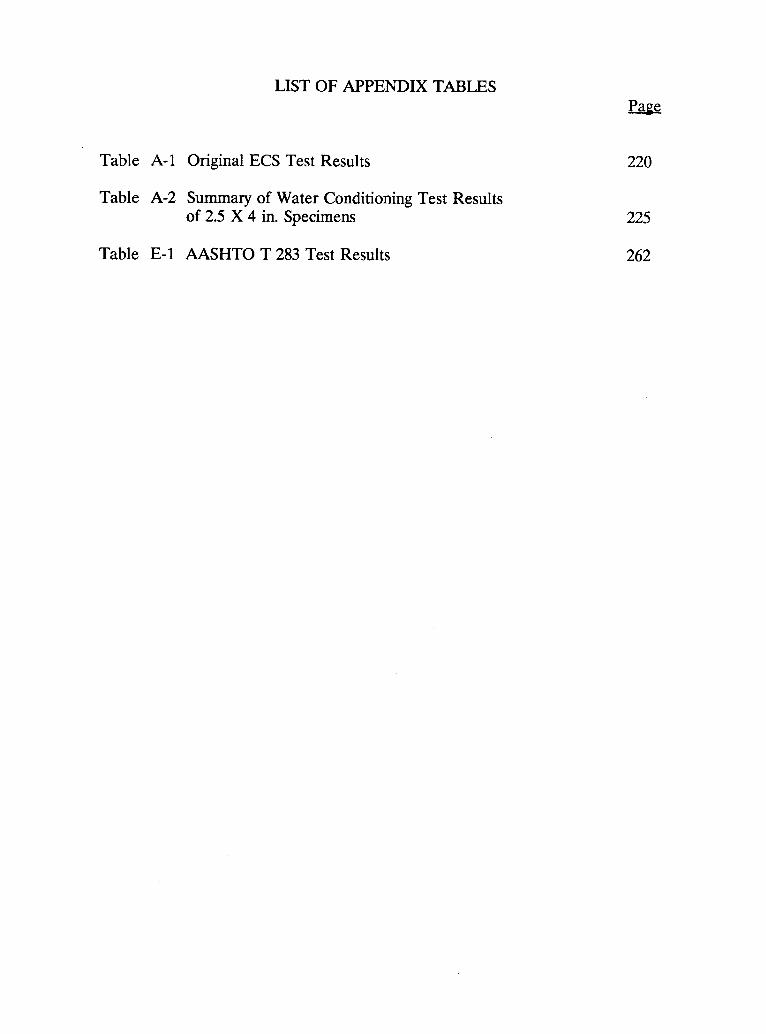
LIST OF APPENDIX TABLES
Table A-1 Original ECS Test Results
Table A-2 Summary of Water Conditioning Test Resultsof 2.5 X 4 in. Specimens
Page
220
225
Table E-1 AASHTO T 283 Test Results 262

DEVELOPMENT OF A TEST PROCEDURE FOR WATERSENSITIVITY OF ASPHALT CONCRETE MIXTURES
1. INTRODUCTION
Environmental factors such as temperature, air (vapor), and water can have a profound
effect on the durability of asphalt concrete mixtures. In mild climates where good quality
aggregates and asphalt cement are available, the major contribution to deterioration may
be due to traffic loading and the resultant distress is manifested in the form of fatigue
cracking, rutting, and raveling. But, when more severe climates are coupled with poor
materials and traffic, premature failure may result.
Although many factors contribute to the degradation of asphalt concrete pavements,
moisture* is a key element in the deterioration of the asphalt mixture. There are three
mechanisms by which moisture can degrade the integrity of an asphalt concrete matrix:
(1) loss of cohesion (or strength) and stiffness of the asphalt film that may
*: The terms moisture and water are often used interchangeably, but there appears to bea difference between the actions of moisture vapor and liquid water on distressmechanisms such as stripping.
2
be due to several mechanisms, (2) the failure of the adhesion (or bond) between the
aggregate and asphalt, and (3) degradation of the aggregate itself. When the
aggregate tends to have a preference for absorbing water, the asphalt is "stripped"
away. This leads to premature pavement distress and ultimately to failure of the
pavement.
The development of tests to determine the water sensitivity of asphalt concrete
mixtures began in the 1930s (Terrel and Shute, 1989). Since that time numerous
tests have been developed in an attempt to identify asphalt concrete mixtures which
are susceptible to water damage. Current test procedures have attempted to simulate
the strength loss (defined as damage) that can occur in the pavement so that asphalt
mixtures which suffer premature distress from the presence of moisture can be
identified prior to construction. An asphalt mixture is identified as being sensitive
to moisture if the laboratory specimen(s) fail a "moisture sensitivity" test. The
implication of the failure is that the particular combination of asphalt, aggregate, and
antistripping additive (if used) would fail before reaching its anticipated design life
due to water-related degradation mechanisms.
The major difficulty in developing a test procedure has been in simulating the field
conditions to which the asphalt concrete is exposed. Environmental conditions,
traffic and time are the factors which need to be accounted for in developing test
procedures to simulate field conditions. Environmental considerations include:
water from precipitation and/or groundwater sources, temperature fluctuations
3
(including freeze-thaw conditions) as well as aging of the asphalt. The effect of
traffic or moving wheel loads could also be considered as an external influence of the
environment. Variability in construction procedures at the time the asphalt mixture
is placed can also influence its performance in the pavement. Since most test
procedures are currently used in the mixture design stage of a project, this variability
adds to the difficulty in predicting field performance. Current test procedures
measure the loss of strength and stiffness, both cohesive and adhesive, of an asphalt
mixture due to water effects. The conditioning processes associated with current test
methods are attempts to simulate field exposure conditions but include acceleration
of the rate of strength loss. Testing of the cohesive and/or adhesive properties which
would identify a moisture susceptible mixture follows the conditioning process.
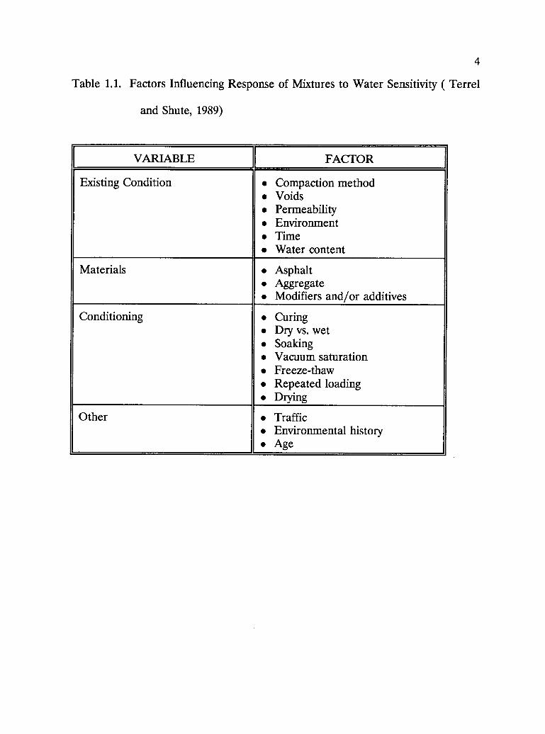
Table 1.1 summarizes those factors that should be considered in evaluating water
sensitivity (Terrel and Shute, 1989).
Moisture sensitivity (or susceptibility) test probably have a "conditioning" and an
"evaluation" phase. The conditioning phases vary, but all of them attempt to simulate
the deterioration of the asphalt concrete in the field. The two general methods of
evaluating "conditioned" specimens are a visual evaluationor subjecting the specimen
to a physical test. In the visual evaluation, observation of the retained asphalt
coating is determined following the conditioning process. Typically, physical test
evaluation includes strength or modulus and a ratio is computed by dividing the
result from the "conditioned" specimen by the result from an "unconditioned"
4
Table 1.1. Factors Influencing Response of Mixtures to Water Sensitivity ( Terrel
and Shute, 1989)
VARIABLE FACTOR
Existing Condition Compaction methodVoidsPermeabilityEnvironmentTimeWater content
Materials AsphaltAggregateModifiers and/or additives
Conditioning CuringDry vs. wetSoakingVacuum saturationFreeze-thawRepeated loadingDrying
Other TrafficEnvironmental historyAge
5
specimen. If the ratio is less than a specified value, the mixture is determined to be
moisture susceptible.
The overal objective of this research addresses the relationship between asphalt
binder properties and the performance of asphalt concrete mixtures. The specific
goal for this thesis is to:
1. Define water sensitivity of asphalt concrete mixtures with respect to
performance, including fatigue, rutting, and thermal cracking.
2. Develop laboratory testing procedures that will predict field
performance.
The scope of this thesis includes a brief summary of the philosophy and
accompanying hypothesis on the nature and effect of water on asphalt paving
mixtures. Following this is the development of these methods, proposed protocols,
and preliminary test results, along with preliminary recommendations.
6
1.1 Background
Test Procedures and Moisture Sensitivity
Numerous methods have been developed to determine if an asphalt concrete mixture
is sensitive to moisture and, therefore, is prone to early water damage. In general,
there are two categories into which the tests can be divided:
1. Tests which coat "standard" aggregate with an asphalt cement with or
without an additive. The loose uncompacted mixture is immersed in
water (which is either held at room temperature or boiled). A visual
assessment of the amount of stripping is estimated.
2. Tests which use compacted specimens, either laboratory compacted or
cores from existing pavement structures. These specimens are
conditioned in some manner to simulate in-service conditions of the
pavement structure. The results of these tests are generally evaluated
by the ratios of conditioned to unconditioned results using a stiffness
or strength test (e.g. diametral resilient modulus test, diametral tensile
strength test, compresive strength, etc.).
7
The use of terms such as "reasonable", "good", and "fair" are often used in
conjunction with the description of how well the results of a test correlate with actual
field performance. Stuart (1986) and Parker and Wilson (1986), found that, for the
tests they evaluated, a single pass/fail criterion could not be established that would
enable the results of the tests to correctly indicate whether or not the asphalt
mixtures they tested were moisture sensitive. These results are characteristic of all
test methods currently used to assess asphalt concrete mixtures for moisture
sensitivity.
From a review of the literature, the following tests have received the most attention
and cover the variety of methods used to evaluate moisture sensitivity, and therefore
were selected for review:
1. NCHRP 246 - Indirect Tensile Test and/or Modulus Test with
Lottman Conditioning
2. NCHRP 274 Indirect Tensile Test with Tunnicliff and Root
Conditioning
3. AASHTO T-283 Combines features of NCHRP 246 and 274
4. Boiling Water Tests (ASTM D 3625)
5. Immersion-Compression Tests (AASHTO T-165, ASTM D 1075)
6. Freeze-Thaw Pedestal Test (Kennedy, et al. 1982).
7. Static Immersion Test (AASHTO T-182, ASTM D 1664)
8
8. Conditioning with Stability Test (AASHTO T-245)
Although not covered in detail in this report, it is apparent from the literature review
and survey of current practice that a variety of test methods have been employed to
assess:
1. The potential for moisture sensitivity in asphalt concrete mixtures, and
2. The benefits offered by antistripping agents to prevent moisture
induced damage to asphalt concrete mixtures.
Conditioning can be accomplished by several methods. Table 1.1 shows a list of
factors or criteria that should be considered when evaluating procedures. A summary
of the methods evaluated was documented in an earlier report (Terrel and Shute
1989). So far, no single test has proven to be "superior" as is evident by the number
and variety of tests currently being used. From the data and experience to date, it
appears that a test has yet to be established that is highly accurate in predicting
moisture susceptible mixtures and estimating the life of the pavement.

9
Philosophy of Water Damage Mitigation
The design of asphalt paving mixtures is a multi-step process of selecting asphalt and
aggregate materials and proportioning them to provide an appropriate compromise
among several variables that affect the mixtures' behavior. Consideration of external
factors such as traffic loading and climate are part of the design process.
Performance factors that are of concern in any design include at least the following
goals:
1. Maximize the fatigue life
2. Minimize the potential for rutting
3. Minimize the effect of low temperature or thermal cycling on cracking
4. Minimize or control the amount and rate of age hardening
5. Reduce the effect of water
In many instances, water or moisture vapor in the pavement can reduce the overall
performance life by affecting any one of the factors listed above. The effect of
stripping or loss of adhesion is readily apparent because the integrity of the mixture
is disrupted. The loss of cohesion is often less obvious, but can cause a major loss
of stiffness or strength. The introduction of air or moisture into the void system
accelerates age hardening, thus further reducing pavement life. The following
discussion is aimed at the evaluation of water sensitivity and mitigation of damage
or loss of performance resulting from water in mixtures.

10
1.2 Hypothesis for Water Damage Mitigation
The effect of water on asphalt concrete mixtures has been difficult to assess, because
of the many variables involved. One of the variables that affects the results of
current methods of evaluation are the air voids in the mixture. The very existence
of these voids as well as their characteristics can play a major role in performance.
Contemporary thinking would have us believe that voids are necessary and/or at least
unavoidable. Voids in the mineral aggregate are designed to be filled to a point less
than full of asphalt cement to allow for traffic compaction. But if one could design
and build the pavement properly, allowing for compaction by traffic would be
unnecessary. In the laboratory, mixtures are designed at, say 4 percent total voids,
but actual field compaction may result in as much as 8 to 10 percent voids. These
voids provide the major access of water into the pavement mixture.
Hypothesis. The existing mixture design method and construction practice tends to
create an air void system in asphalt concrete that may be a major cause of moisture
related damage.
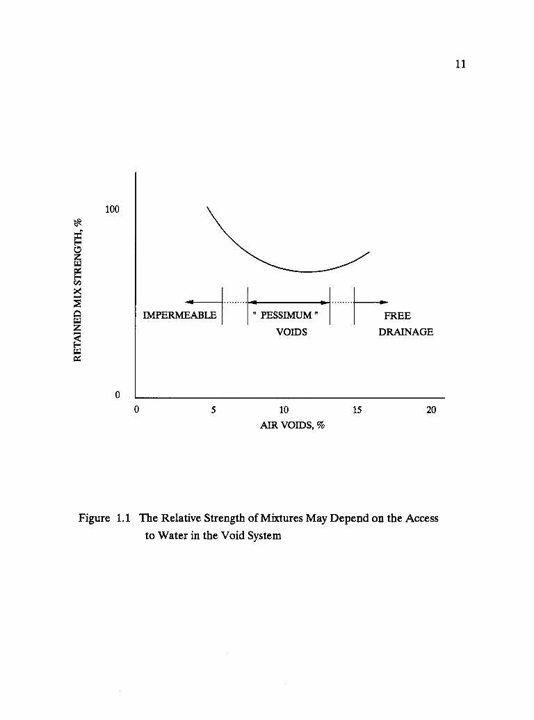
A major effect of air voids is illustrated in Figure 1.1. If mixtures of asphalt concrete
were prepared and conditioned by some process such as water saturation followed
by freezing and thawing, it can be shown that the retained strength or modulus is
typically somewhat lower than for the original dry mixture. However, this effect
11
e
W
c)X2
E-iWrx
100
0
-..
IMPERMEABLE " PESSIMUM "
VOIDS
FREE
DRAINAGE
0 5 10 15 20
AIR VOIDS, %
Figure 1.1 The Relative Strength of Mixtures May Depend on the Access
to Water in the Void System
12
tends to be tempered by the voids in the mixture, particularly access to the voids by
water. If the mixtures shown in Figure 1.1 were designed for a range of voids by
adjusting the aggregate size and gradation and the asphalt content, a range of
permeability would result. Those mixtures with minimal voids that are not
interconnected would be essentially impermeable. When air voids increased beyond
some critical value they would become larger and interconnected, thus water could
flow freely through the mixture. Between these two extremes of impermeable and
open or free draining mixtures is where most asphalt pavements are constructed.
The voids tend to range from small to large, with a range of permeability depending
on their interconnection.
The curve in Figure 1.1 indicates that the worst behavior in the presence of water
should occur in the range where most conventional mixtures are compacted. Thus,
the term "pessimum voids" can be used to describe a void system (i.e., the opposite
of optimum). Pessimum voids can actually represent a concept of quantity (amount
of voids in the mixture) and quality (size, distribution, and interconnection) as they
affect the behavior and performance of pavements.
Intuitively, one could equate the three regions in Figure 1.1 as follows:
1. Impermeable or low void mixtures are made with high asphalt content
or are mastics. To offset the instability expected from high binder
13
content, aggregate gradation is modified (crushed sand, large size
stone) and an improved binder containing polymers and/or fibers can
be used.
2. The mid-range or pessimum voids is represented by conventional
"dense graded" asphalt concrete as used in the U.S.
3. Free draining or open graded mixtures are designed as surface friction
courses or draining base courses. With the use of polymer modified
asphalt, these mixtures can be designed with higher binder content
(thicker films) to remain open and stable under traffic.
The European community has recognized the advantages of mixtures that fall outside
the pessimum voids region (Die Asphaltstrasse, June 1989) in an investigation of
"Stone-Mastic Asphalt" and "Porous Asphalt". The stone-mastic mixtures have high
stability combined with very good durability, have low voids (3 to 4 percent) and
increased performance life (20 to 40 percent) compared to conventional dense
graded mixtures. Porous asphalt is widely also used in Europe to improve safety,
reduce noise and spray from tires. With the use of polymer modified asphalt,
durability is increased and performance life is increased from seven to more than 12
years (Shute, et al. 1989).
14
Theory for Water Sensitivity Behavior
As indicated earlier, water appears to affect asphalt concrete mixtures through two
major mechanisms: (1) loss of adhesion between the asphalt binder and aggregate
surface, and (2) loss of cohesion through a gross "softening" of the bitumen or
weakening of asphalt concrete mixtures.
Voids in the asphalt concrete are the most obvious source of entry of water into the
compacted mixture. Once a pavement is constructed, the majority of water and air
ingress is through these relatively large voids. Other voids or forms of porosity may
also affect water sensitivity. For example, aggregate particles have varying sizes and
amounts of both surface and interior voids. Water trapped in the aggregate voids
due to incomplete drying plays a role in coating during construction and during its
early service life. Also, there appears to be some indication that asphalt cements
may themselves absorb water and/or allow some water to pass through films at the
aggregate surface. The complexity of the water-void system will require a careful and
detailed evaluation to better understand its significance.
Although continued study of water sensitivity will very likely result in improved
understanding and performance, the starting point or state of the art is a good
beginning.
15
Theories of Adhesion
Shute et al. (1989) has provided a good overview of previous research and current
thinking on adhesion. Four theories of adhesion have been developed around several
factors that appear to affect adhesion, namely:
1. Surface tension of the asphalt cement and aggregate
2. Chemical composition of the asphalt and aggregate
3. Asphalt viscosity
4. Surface texture of the aggregate
5. Aggregate porosity
6. Aggregate cleanliness, and
7. Aggregate moisture content and temperature at the time of mixing
with asphalt cement
No single theory seems to completely explain adhesion; it is most likely that two or
more mechanisms may occur simultaneously in any one mixture, thus leading to loss
of adhesion. In summary, the four theories of adhesion are as follows:
Mechanical Adhesion relies on several aggregate properties including surface texture,
porosity or absorption, surface coatings, surface area, and particle size. In general,
a rough, porous surface appears to provide the strongest interlock between aggregate
16
and asphalt. Some absorption of asphalt into surface voids provides a mechanical
interlock as well as additional surface area.
Chemical Reaction is recognized as a possible mechanism between asphalt cement
and aggregate surfaces. Many researchers have noted that better adhesion may be
achieved with basic aggregates compared to acidic aggregates. However, very
acceptable mixtures have been produced using all types of aggregates. More recent
work in the Strategic Highway Research Program (SHRP) program (Auburn
University) is concentrating on the chemical interactions at the aggregate-asphalt
interface (Curtis et al, 1991).
Surface Energy theory is used in an attempt to explain the relative wettability of
aggregate surfaces by asphalt and/or water. Water is a better wetting agent than
asphalt because it has a lower viscosity and lower surface tension. When asphalt
coats aggregate, a change of energy, termed adhesion tension, occurs that is related
to the mutual affinity of asphalt cement and aggregates.
Molecular Orientation theory suggests that molecules of asphalt align themselves
with unsatisfied energy changes on the aggregate surface. Although some molecules
in asphalt are di-polar, water is entirely di-polar and this may help explain the
preference of aggregate surfaces for water rather than asphalt.
17
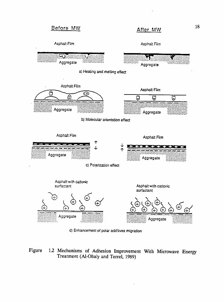
All of the above mechanisms may occur to some extent in any asphalt-aggregate
system. As part of a study on microwave effects, Al-Ohaly and Terrel (1988) have
summarized the various mechanisms as shown in Figure 1.2. Aside from the
suggested microwave heating effects, several improvements can be visualized:
mechanical interlock, molecular orientation, and polarization.
Research has shown that adhesion can be improved through the use of various
commercial liquid antistrip additives as well as lime.
Theories of Cohesion
In compacted asphalt concrete, cohesion might be described as the overall integrity
of the material when subjected to load or stress. Assuming that adhesion between
aggregate and asphalt is adequate, cohesive forces will develop in the asphalt film or
matrix. Generally, cohesive resistance or strength might be measured in a stability
test, resilient modulus test, or tensile strength test. The cohesion values are
influenced by factors such as viscosity of the asphalt-filler system. Water can affect
cohesion in several ways such as through intrusion into the asphalt binder film and
through saturation and even expansion of the void system (swelling). Although the
effects of stripping may also occur in the presence of water, a mechanical test such
Before MW
Asphalt Film
........Aggregate -
After MW
Asphalt Film
a) Heating and melting effect
Asphalt Film
e+)
Aggregate
Asphalt Film
Aggregate
Asphalt Film
b) Molecular orientation effect
IMIM WM, IMMO. es.= .1 4B Imo
Aggregate
c) Polarization effect
Asphalt with cationicsurfactant
-b le, 46- ei
Aggregate
4,
. . . . . . ....
Aggregate
Asphalt Film
411. 4. 4 4. 4 4.
Aggregate
Asphalt with cationicsurfactant
d) Enhancement of polar additives migration
Aggregate -
18
Figure 1.2 Mechanisms of Adhesion Improvement With Microwave EnergyTreatment (Al-Ohaly and Terre!, 1989)
19
as repeated load resilient modulus tends to measure gross effects and the
mechanisms of adhesion or cohesion cannot be distinguished separately.
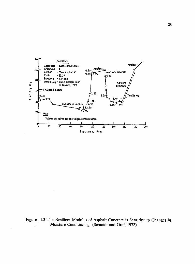
On a smaller scale, in the asphalt film surrounding aggregate particles, cohesion can
be considered the deformation or resistance to deformation under load that occurs
at some distance from the aggregate surface - beyond the influence of mechanical
interlock and molecular orientation. An example of the effect of water on cohesion
(i.e., resilient modulus) is shown in Figure 1.3. This early work by Schmidt and Graf
(1972) illustrates that a mixture will lose about 50 percent of its modulus upon
saturation with water. The loss may continue with time, but at a slower rate while
it remains wet. Upon drying, the modulus was completely restored, and a further
repetition of wetting and drying resulted in the same behavior. Over the 6 + month
period of the conditioning process, there appeared to be a slight overall stiffening,
that is probably due to age hardening of the asphalt cement. The observation made
from data such as in Figure 1.3 helps in providing a better understanding of the
effects of water on mixture performance.
120
100o-
800-
Conditions
Aggregate - Cache Creek Crave!Gradation - IAsphalt - 5% of Asphalt CVoids -13.3%Exposure - VariableType of MR Direct Compression
or Tension, 73'F
el3...
...", Vacuum Saturate60e. 5.6%
Aao
20Note
Values on points are the weight percent water.
0.3%0.
Ambient
0.$
1.116.0%
1.75Vacuum Desiccate 1.91
3.7%
C.61
Vacuum Saturate
5.2%
Ambien
Ambient ,Desiccate /i
/ Tensile MR
: /..//6.3% 1r
//
0 I I0 20 40 60 $0 100 120 140 160 180 200
Exposure. Days
20
Figure 1.3 The Resilient Modulus of Asphalt Concrete is Sensitive to Changes inMoisture Conditioning (Schmidt and Graf, 1972)
21
1.3 Research Objectives
Keeping in mind the two-fold goal, this research is focused on investigating the most
important factors influincing the water sensitivity and the development of a test
procedure to assist in evaluating water sensitivity.
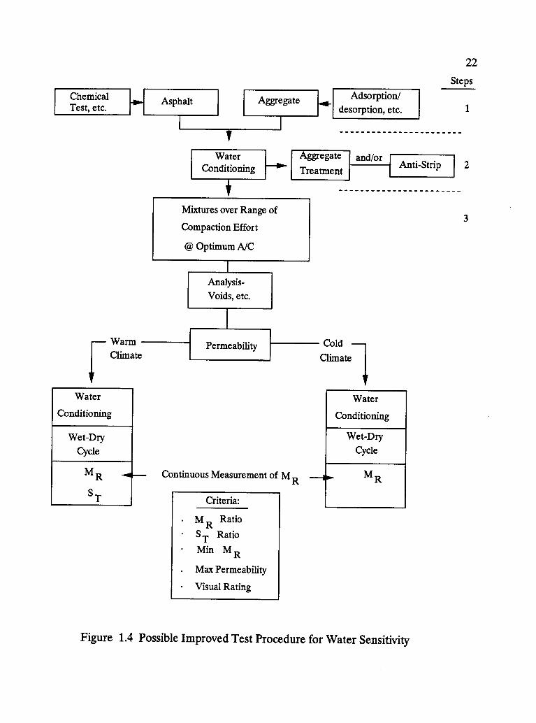
A materials evaluation procedure for routine use might take several different forms,
but the one initially envisioned for this project includes three separate steps as
follows:
Step 1. Testing and screening of potential materials, both aggregates
and asphalt binders to eliminate those candidates with non-
compatible properties such as a high tendency toward stripping.
Step 2. Mixing aggregates and asphalt together and testing the loose
mixtures for adhesion, particularly stripping.
Step 3. Testing compacted mixtures to evaluate the overall sensitivity
to water and their potential for successful performance in
pavements.
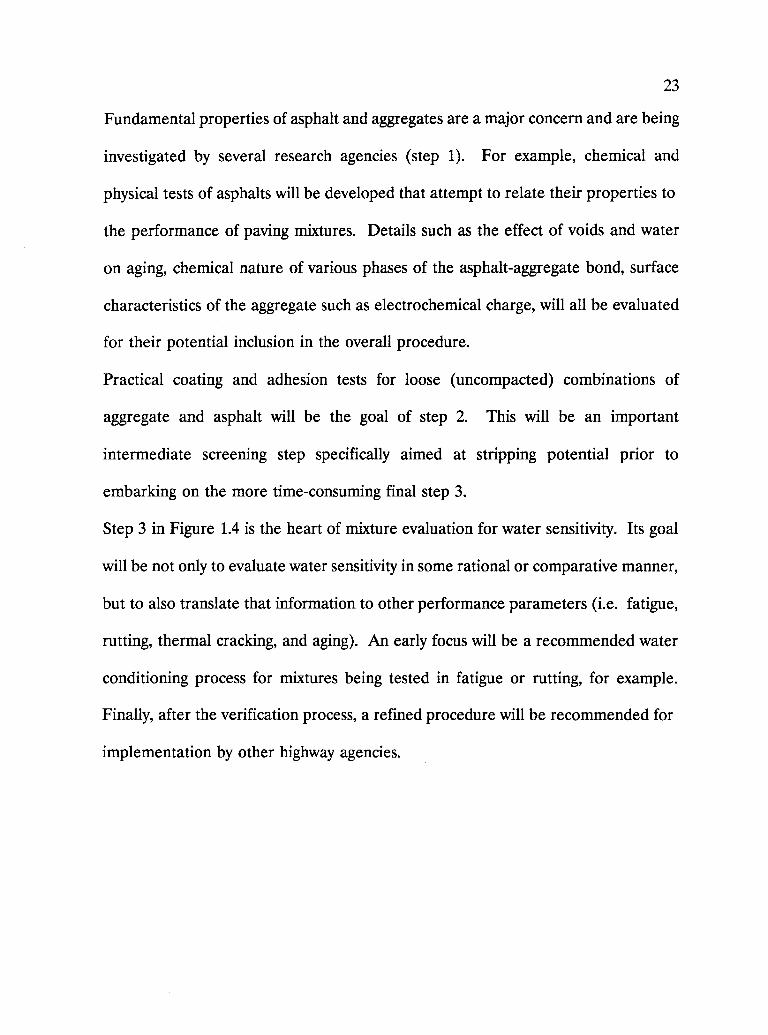
Figure 1.4 is a diagram showing these steps in the right-hand margin and more
details of the procedure are outlined within the figure.
ChemicalTest, etc.
WarmClimate
Water
Conditioning
Wet-DryCycle
M R
ST
Asphalt Aggregate
v
WaterConditioning
Adsorption/desorption, etc.
22
Steps
Aggregate
Treatmentand/or
Mixtures over Range of
Compaction Effort
@ Optimum A/C
Analysis-
Voids, etc.
Permeability
Continuous Measurement of MR
Criteria:
MR
Ratio
ST Ratio
Min M R
Max Permeability
Visual Rating
Anti-Strip
Cold
Climate
Water
Conditioning
Wet-DryCycle
M R
Figure 1.4 Possible Improved Test Procedure for Water Sensitivity
1
2
3
23
Fundamental properties of asphalt and aggregates are a major concern and are being
investigated by several research agencies (step 1). For example, chemical and
physical tests of asphalts will be developed that attempt to relate their properties to
the performance of paving mixtures. Details such as the effect of voids and water
on aging, chemical nature of various phases of the asphalt-aggregate bond, surface
characteristics of the aggregate such as electrochemical charge, will all be evaluated
for their potential inclusion in the overall procedure.
Practical coating and adhesion tests for loose (uncompacted) combinations of
aggregate and asphalt will be the goal of step 2. This will be an important
intermediate screening step specifically aimed at stripping potential prior to
embarking on the more time-consuming final step 3.
Step 3 in Figure 1.4 is the heart of mixture evaluation for water sensitivity. Its goal
will be not only to evaluate water sensitivity in some rational or comparative manner,
but to also translate that information to other performance parameters (i.e. fatigue,
rutting, thermal cracking, and aging). An early focus will be a recommended water
conditioning process for mixtures being tested in fatigue or rutting, for example.
Finally, after the verification process, a refined procedure will be recommended for
implementation by other highway agencies.
24
2. EXPERIMENT DESIGN
This study is aimed at determining the factors that most influence water sensitivity
of asphalt paving mixtures. A logical approach is to study the fundamental properties
of asphalt and aggregate, as shown in Table 1.1, and develop a series of tests that
would rate or screen various combinations for probability of successful performance.
The basic factors that influence compacted mixtures such as permeability, time, and
rate of wetting or saturation, aging, etc., would then be evaluated for a range of
mixtures. Since the permeability (or air voids) is a major factor affecting mixture
behavior, it is used as a controlled variable in the experiment plan (as discussed
later) to characterize the response of asphalt concrete specimens to the change in
water conditioning factors as time, and rate of wetting, and temperature cycling.
Eventually, a water conditioning and testing procedure would be recommended for
testing by various user agencies prior to final standardization.
25
2.1 Variables
The development of tests to determine the water sensitivity of asphalt concrete
mixtures began in the 1930s. Since that time, interest in the effect of water sensitivity
on life and performance of asphalt concrete pavements has increased and numerous
test procedures have been developed in an attempt to understand the phenomenon
of adhesion and cohesion between asphalt cement and mineral aggregate.
Test procedures have attempted to simulate the strength loss or other damage that
can occur in the pavement so that asphalt mixtures which suffer premature distress
from the presence of moisture or water can be identified prior to construction. An
asphalt mixture is identified as being sensitive to water if the laboratory specimens
fail a moisture sensitivity test. The implication of the failure is that this particular
combination of asphalt and aggregate would fail due to water related mechanisms
before reaching its anticipated design life.
Simulating the field conditions to which the asphalt concrete is exposed has been the
most difficult in all water sensitivity tests. A water sensitivity protocol includes two
major phases; a conditioning and an evaluation phase. The conditioning phases vary,
but all of them attempt to simulate the performance of the asphalt concrete in the
field with presence of water. The two general methods of evaluating conditioned
specimens are visual evaluation and/or subjecting the specimen to a physical test.
The objective of this research is to develop a laboratory conditioning procedure
(moisture, temperature, load) to be used for water sensitivity evaluation during the
26
design process and for conditioning prior to testing in other modes, such as fatigue,
rutting, aging, and thermal cracking.
It is not only important to simulate the pavement conditions in the laboratory, but
also to take into consideration the effect of the environment over a long period of
time. In this study, the laboratory tests and their condition factors were selected with
greater care to represent the realistic conditions of the asphalt pavement in real
service. Table 2.1 summarizes the factors included in this research which influence
response of asphalt concrete to water sensitivity.
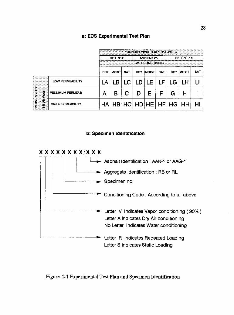
In order to conduct the research, it was necessary to design an experimental testing
program which includes all related variables. Figure 2.1 shows a 3x3 factorial-design
experiment. This testing program was conducted by using the Environmental
Conditioning System (ECS). The controlled variables and their treatment levels
incorporated in the factorial design experiment were:
1. Temperature with three treatment levels:
Hot: 60°C (140°F)
Ambient: 25 °C (77°F)
Freeze: -18°C (0°F)

27
Table 2.1 Factors Considered in The Experiment Plan
Variable Factor
Materials AsphaltAggregate
ExistingCondition
CompactionVoidsPermeabilityEnvironmentTimeWater content
ConditioningDry vs. wetVacuum saturationTemperature CyclingRepeated loadingDrying
28
a: ECS Experimental Test Plan
........................................................ ......
HOT 80 C AMBIENT 25 FREEZE -18
:CONDIT40
DRY MOIST SAT. DRY MOIST SAT. DRY MOIST SAT.
LOW PERMEABIUTY LA LB LC LD LE LF LG LH LI
PESSIMUM PERMEAB. A B C D E F G H
HIGH PERMEABILITY HA HB HC HD HE HF HG HH HI
b: Specimen identification
X X X X X X X X/XX X
1 Asphalt Identification : AAK-1 or AAG-1
Aggregate Identification : RB or RL
Specimen no.
Conditioning Code : According to a: above
Letter V Indicates Vapor conditioning ( 90% )
Letter A Indicates Dry Air conditioning
No Letter Indicates Water conditioning
Letter R Indicates Repeated LoadingLetter S Indicates Static Loading
Figure 2.1 Experimental Test Plan and Specimen Identification
29
2. Permeability with three treatment levels depending on the air voids
(AV):
Low permeability (% AV 56)
Pessimum permeability (6 < %AV < 14)
High permeability (% AV 14)
3. Wet conditioning with three treatment levels defined as follows:
Dry: No water conditioning
Moist: By running water through the specimens at 25 °C under
10 inches of Hg vacuum for 30 min.
Wet: By running water through the specimen at 25 °C under 20
inches of Hg vacuum for 30 min.
After most of the preliminary tests and mini-studies were complete, a modified test
plan was initiated. During the early stages of laboratory testing, it became apparent
that it is not necessary to perform all of the dry and ambient conditionings, Figure
2.1, where conditioning only one of each to show the boundaries of the conditioning
variables is appropriate. The temperatures used for conditioning were limited to the
extremes of 60°C and -18°C, with the intermediate 25 °C range used only for limited
comparisons. Early testing showed that the dry conditioning resulted in aging, which
is expected, so only moist and wet were used, with the dry range used only to show
the boundaries of moisture conditioning. The high air voids level was investigated
only after modifying the test setup to overcome some of the problems associated with
conditioning very high air void specimens at high temperatures.
30
The details of the test results of conditioning high air void specimens are discussed
in a separate section about proving the pessimum voids hypothesis.
In summary, most of the testing reported under this experiment plan is confined to
two void or permeability levels, hot or freezing temperatures and moist or wet
moistures. Three conditioning cycles were used for the entire experiment, applying
repeated loading during all the conditioning cycles except the freezing cycles.
Determination of Saturation Level
A suitable degree of saturation based on AASHTO T-283 and other previous
experience, Lottman (1988), was established to be between 55% and 80% of the
volume of air. This target window of saturation was achieved by placing the
specimen in a vacuum container filled with distilled water and applying a partial
vacuum, such as 20 inches Hg, for a short time. If the degree of saturation was not
within the limits, adjustments could be made by trial and error by changing vacuum
level and/or submerging time. This saturating method worked satisfactorily for
asphalt concrete mixtures, 8%±1% air voids.
The ECS method (as discussed later) attempted to standardize the wetting procedure
by controlling water accessibility and vacuum level, instead of controlling water
volume and degree of saturation, as in T-283.
31
The ECS uses a controlled vacuum for saturation by maintaining the desired vacuum
level during the wetting stage according to the experimental plan and a 10-in vacuum
level during the conditioning cycles, while some of the current methods, such as
AASHTO T 283, use a controlled degree of saturation by maintaining the degree of
saturation between 50 and 80 percent. In the case of similar gradations with one air
voids level, using the controlled degree of saturation technique is appropriate. But
since the objective of this study is to come up with a universal water conditioning
procedure for asphalt mixtures with different air voids, using the controlled degree
of saturation is not the best, as there are dense mixtures where 60 percent of their
air voids are not connected or unaccessible, and in this case it is not possible to
achieve the min. 50 percent saturation with any high vacuum level. Also on the other
extreme, there are open graded mixtures with air voids such as 14 percent or more,
where almost all the air voids are interconnected and very accessible to water. By
only soaking or dipping the specimens in the water bath without applying vacuum,
they will get more than 90 percent of saturation.
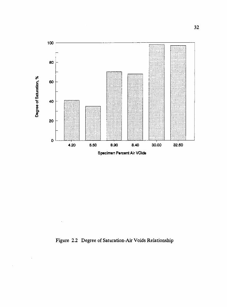
In order to illustrate the above concept, three sets of specimens with three levels of
air voids, 4, 8, and 31 percent, were placed in a vacuum container and partially
saturated under the effect of a 20-in. vacuum level for 30 minutes. Figure 2.2 shows
the degree of saturation-air voids relationship under the same vacuum level. This
confirms that in order to achieve a target saturation level for a specimen with certain
air void levels, one may inadvertently destroy the specimen because of the need for
the high vacuum level, as in the case of low 4 percent air voids.
100
80
60
40
20
0
32
4.20 5.50 8.90 8.40 30.00
Specimen Percent Air VOids
32.60
Figure 2.2 Degree of Saturation-Air Voids Relationship
33
In contrast, one may achieve the target degree of saturation before reaching an
appropriate accelerated wetting process, such as the case of 31 percent air voids.
Based on this, for the ECS the water penetration into the mixture was used as a
saturation indication, rather than the volume of water. This results in using the
controlled vacuum, which actually controls the water penetration.
The ECS testing experiment was conducted on the following materials and loading
conditions:
1. Two asphalt types,
2. Two aggregate types,
3. Two loading levels.
Originally, specimen height was 2.5 inches as in a conventional Marshall briquet.
After gaining experience, it was observed that measurement of the resilient modulus
from 2.5 in. specimens had poor repeatability. Thus, a specimen 4 in. in height and
4 in. in diameter was recommended (see Chapter 3 for more information on the
ECS-MR) for better repeatability. All the results from short specimens are included
in Appendix A for general information but they are not used in the analysis and
development of conclusions. The test results of 4-inch height specimens are included
in Chapter 3.
34
The effectiveness of each controlled variable, see Table 2.1, was determined from the
values of response variables. Response variables are as follows:
1. Resilient modulus, MR, change (retained or gained MR) ratio from
original MR.
2. Permeability, K, change (retained or gained permeability) ratio from
original permeability.
3. Visual evaluation the percentage of retained asphalt coating on the
aggregate for conditioned specimens.
Finally, upon completing this research on water sensitivity of asphalt concrete
mixtures, four goals were achieved:
1. Development of the Environmental Conditioning System (ECS) as a
conditioning and testing device.
2. Evaluation of ECS
3. Recommended WET conditioning procedure as a water conditioning
prior to testing in fatigue, rutting, and low temperature cracking.

35
4. Recommended a new water conditioning procedure for evaluating
water sensitivity as a part of mix design, i.e., Mix Design and Analysis
System (MIDAS).
2.2 Equipment and Procedures
In order to test the above hypothesis and variables, discussed in Chapter 1, the
Environmental Conditioning System (ECS) was designed and fabricated to assist in
determining the most important factors in the performance of mixtures in the
presence of moisture,as shown in Table 2.1. The test set-up will permit evaluation
of air voids and behavior of mixtures in several ways, including:
1) Saturation versus wet (partial saturation)
2) Water versus vapor
3) Permeability versus air void content
4) Freezing versus no freezing
5) Volume change effects (i.e., "oversaturation")
6) Effects of time on rate of saturation or desaturation
7) Continuous monitoring using MR
8) Dynamic loading versus static loading
9) Coating and stripping

36
It is expected that the ECS can be used to evaluate the above factors in terms of the
effectiveness of currently used testing procedures as well as lead to the development
of a new testing procedure. In addition, the ECS will be used to assist in the
validation of concepts developed by SHRP asphalt research. As noted above, the
ECS has the capability to test a wide range of factors, but it is recognized that all of
this capability may not be required in the final version of the ECS test to be used for
routine mix design testing (MIDAS).
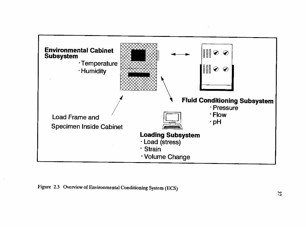
Testing System
The Environmental Conditioning System (ECS) was designed and fabricated to
provide a means of simulating various conditions within an asphalt pavement.
Figure 2.3 shows the ECS and its subsystems:
1. fluid conditioning,
2. environmental conditioning cabinet, and
3. loading system
Environmental CabinetSubsystem
* Temperature*Humidity
Load Frame and
Specimen Inside Cabinet
Fluid Conditioning Subsystem* Pressure* Flow* pH
Loading Subsystem* Load (stress)* Strain* Volume Change
Figure 2.3 Overview of Environmental Conditioning System (ECS)
38
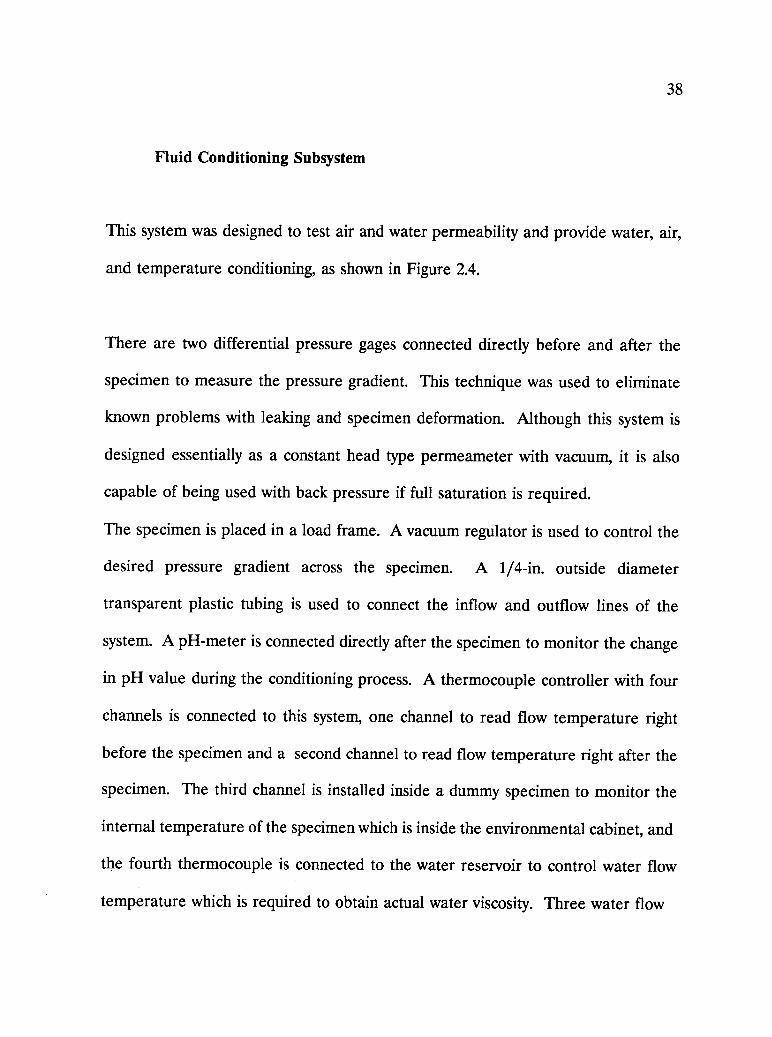
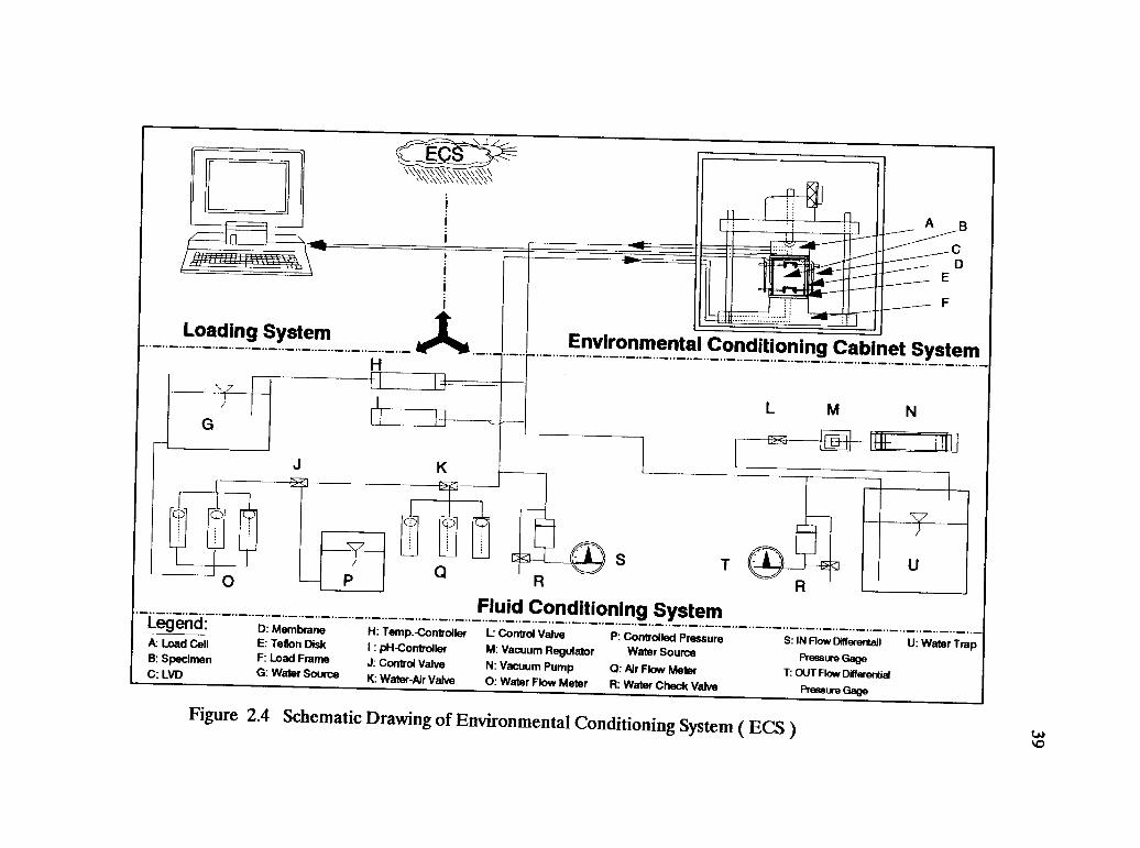
Fluid Conditioning Subsystem
This system was designed to test air and water permeability and provide water, air,
and temperature conditioning, as shown in Figure 2.4.
There are two differential pressure gages connected directly before and after the
specimen to measure the pressure gradient. This technique was used to eliminate
known problems with leaking and specimen deformation. Although this system is
designed essentially as a constant head type permeameter with vacuum, it is also
capable of being used with back pressure if full saturation is required.
The specimen is placed in a load frame. A vacuum regulator is used to control the
desired pressure gradient across the specimen. A 1/4-in. outside diameter
transparent plastic tubing is used to connect the inflow and outflow lines of the
system. A pH-meter is connected directly after the specimen to monitor the change
in pH value during the conditioning process. A thermocouple controller with four
channels is connected to this system, one channel to read flow temperature right
before the specimen and a second channel to read flow temperature right after the
specimen. The third channel is installed inside a dummy specimen to monitor the
internal temperature of the specimen which is inside the environmental cabinet, and
the fourth thermocouple is connected to the water reservoir to control water flow
temperature which is required to obtain actual water viscosity. Three water flow
Loading SystemEnvironmental Conditioning Cabinet System
Legend:A: Load Cell13: Specimen
C: LVD
D: Membrane H: Temp.-ControllerE: Teton DiskF: load FrameG: Water Source
I : pH-Controller
J: Control Valve
K: Water-Air Valve
R
Fluid Conditioning SystemL Control Valve P: Controlled PressureM: Vacuum Regulator Water SourceN: Vacuum Pump Q: Air Flow Meter0: Water Flow Meter R: Water Check Valve
S: IN Flow DNferentail U: Water TrapPressure Gage
T: OUT Flow Differential
Pressure Gage
Figure 2.4 Schematic Drawing of Environmental Conditioning System ( ECS )
40
meters of different flow capacities are connected to a fluid water conditioning system
to provide a sufficiently wide flow range, from 1 to 3000 cm3 /min and another three
air flow meters are also connected to the system to read a total range from 100 to
70,000 cm3/min.
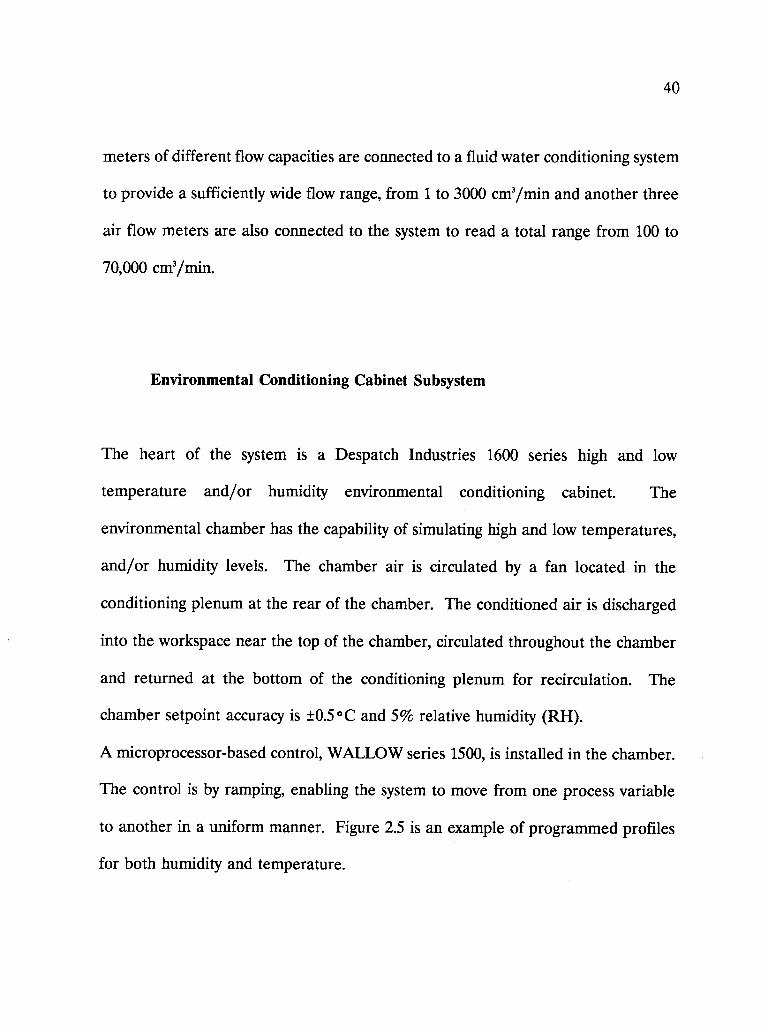
Environmental Conditioning Cabinet Subsystem
The heart of the system is a Despatch Industries 1600 series high and low
temperature and/or humidity environmental conditioning cabinet. The
environmental chamber has the capability of simulating high and low temperatures,
and/or humidity levels. The chamber air is circulated by a fan located in the
conditioning plenum at the rear of the chamber. The conditioned air is discharged
into the workspace near the top of the chamber, circulated throughout the chamber
and returned at the bottom of the conditioning plenum for recirculation. The
chamber setpoint accuracy is ±0.5 °C and 5% relative humidity (RH).
A microprocessor-based control, WALLOW series 1500, is installed in the chamber.
The control is by ramping, enabling the system to move from one process variable
to another in a uniform manner. Figure 2.5 is an example of programmed profiles
for both humidity and temperature.
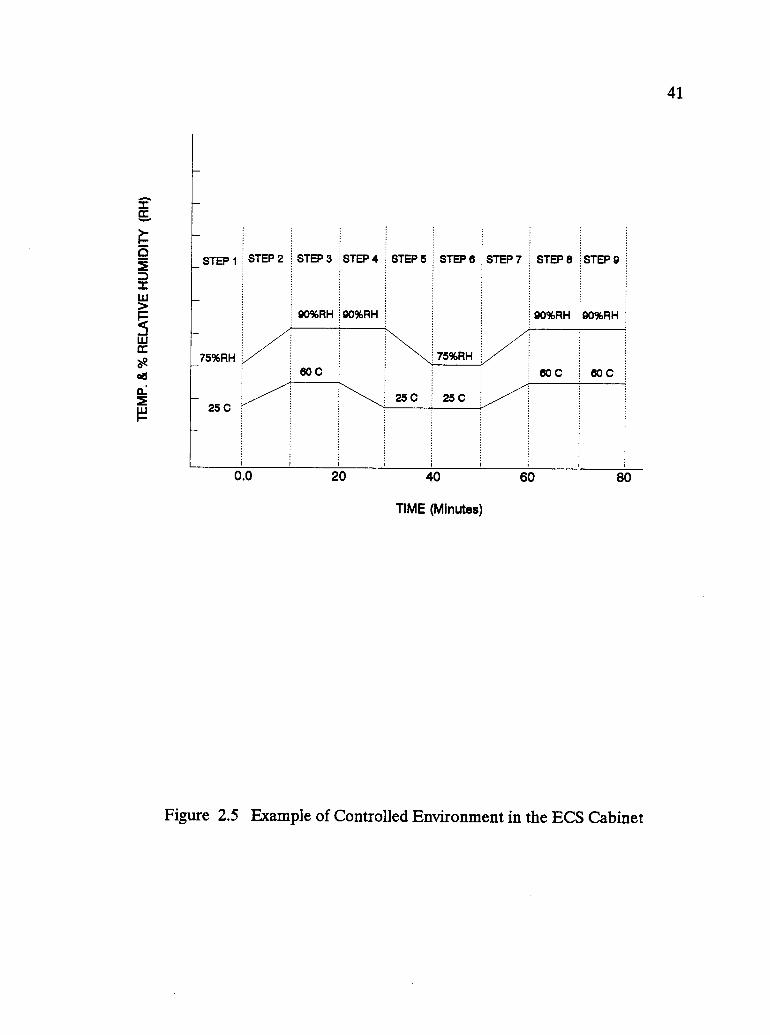
STEP 1
75%RH
25 C
STEP 2 STEP 3 STEP 4
90%RH 90%RH
80C
STEP 5
25 C
STEP
75%RH
25 C
STEP 7 STEP 8 STEP 9
90%RH 90%RH
W C 80 C
0.0 20 40 60 80
TIME (Minutes)
Figure 2.5 Example of Controlled Environment in the ECS Cabinet
41
42
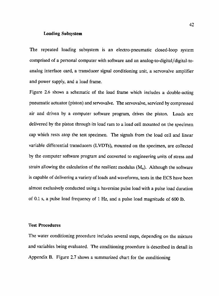
Loading Subsystem
The repeated loading subsystem is an electro-pneumatic closed-loop system
comprised of a personal computer with software and an analog-to-digital/digital-to-
analog interface card, a transducer signal conditioning unit, a servovalve amplifier
and power supply, and a load frame.
Figure 2.6 shows a schematic of the load frame which includes a double-acting
pneumatic actuator (piston) and servovalve. The servovalve, serviced by compressed
air and driven by a computer software program, drives the piston. Loads are
delivered by the piston through its load ram to a load cell mounted on the specimen
cap which rests atop the test specimen. The signals from the load cell and linear
variable differential transducers (LVDTs), mounted on the specimen, are collected
by the computer software program and converted to engineering units of stress and
strain allowing the calculation of the resilient modulus (MR). Although the software
is capable of delivering a variety of loads and waveforms, tests in the ECS have been
almost exclusively conducted using a haversine pulse load with a pulse load duration
of 0.1 s, a pulse load frequency of 1 Hz, and a pulse load magnitude of 600 lb.
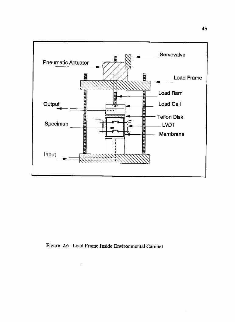
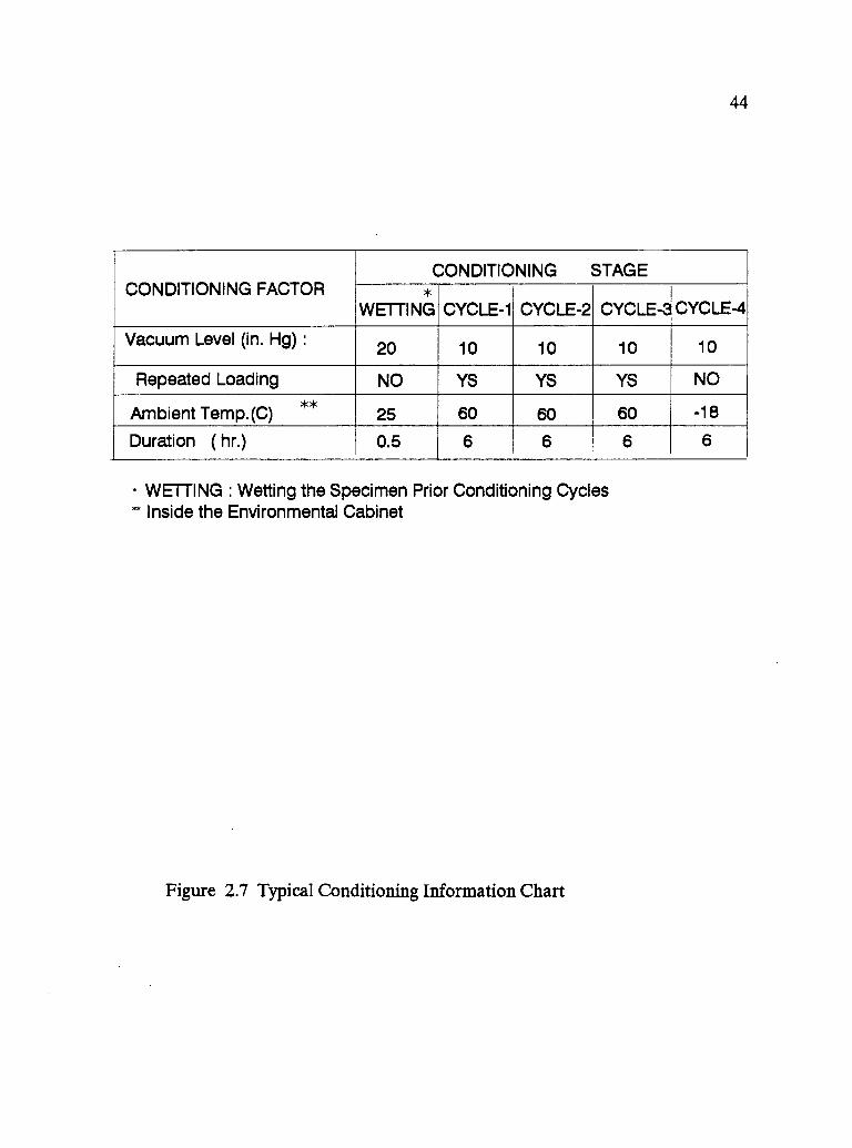
Test Procedures
The water conditioning procedure includes several steps, depending on the mixture
and variables being evaluated. The conditioning procedure is described in detail in
Appendix B. Figure 2.7 shows a summarized chart for the conditioning
43
Pneumatic Actuator
Output
Specimen
Input
Servovalve
Load Frame
Load Ram
Load Cell
Teflon Disk
LVDT
Membrane
Figure 2.6 Load Frame Inside Environmental Cabinet
44
CONDITIONING FACTORCONDITIONING STAGE
*WETTING CYCLE-1 CYCLE-2 CYCLE-CYCLE-4
Vacuum Level (in. Hg) : 20 10 10 10 10
Repeated Loading NO YS YS YS NO
Ambient Temp. (C) ** 25 60 60 60 -18
Duration ( hr.) 0.5 6 6 6 6
* WETTING : Wetting the Specimen Prior Conditioning Cycles- Inside the Environmental Cabinet
Figure 2.7 Typical Conditioning Information Chart

45
variables. Mainly, each test procedure includes three stages. First is the evaluation
of the specimen in dry conditions by performing the dry "original" resilient modulus
(MR) and permeability (k) tests. Second is the "wetting stage" by running water
through the specimen for 30 minutes under the effect of the desired vacuum level
(either 10-in or 20-in.). The wetting procedure is described in detail in Appendix C.
Third, the conditioning stage includes three 6-hour cycles with maintaining a 10-in.
vacuum and continuous repeated loading on the specimen during the conditioning
cycles. In the case of freeze cycles, there is no repeated loading was performed, but
the 10-in. vacuum is maintained, which is equivalent to 5 psi. Loading of the
conditioning cycles with 10-in. vacuum and without a continuous repeated loading is
identified as static loading. In summary, the steps of the conditioning procedure can
be summarized as follows:
1) A 4-in. diameter by 4-in. high specimen is mixed and compacted
2) Physical measurements, density, voids, etc. determined.
3) Preconditioned resilient modulus determined.
4) Circumferential silicon seal applied, specimens mounted in load frame.
5) Measure (air) permeability.
6) LVDs mounted.
7) "Wet" specimen according to desired procedure and measure (water)
permeability.
8) Begin conditioning cycles according to the desired sequence.
Figure 2.7 shows a typical conditioning chart that is used for each test.
46
9) The resilient modulus (MR) and water permeability (k) are measured
following each cycle at 25 ° C.
10) Split open specimen.
11) Observe and report stripping rate.
2.3 Materials
Two aggregates and two asphalts were used from the Materials Reference Library
(MRL) at the University of Texas (Austin). The two aggregates and two asphaltsare
as follows:
1. Aggregates: Watsonville granite, RB, a non-stripper and Gulf Coast
gravel, RL, a stripper.
2. Asphalts: Boscan, AAG-1, and California Valley, AAK-1. These were
selected because of their vastly different compositional and
temperature-susceptibility characteristics.
From these two asphalts and two aggregates four asphalt-aggregate combinations
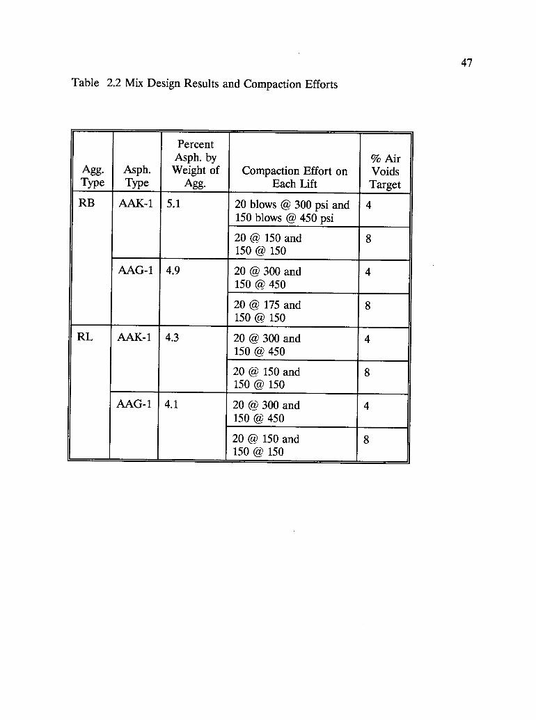
were used to fabricate mixtures. Table 2.2 shows asphalt content for each mixture
which was compacted using kneading compactor (ASTM D 1561), ASTM D 1560,
(see Appendix D for sample preparation protocol). For the two aggregates,
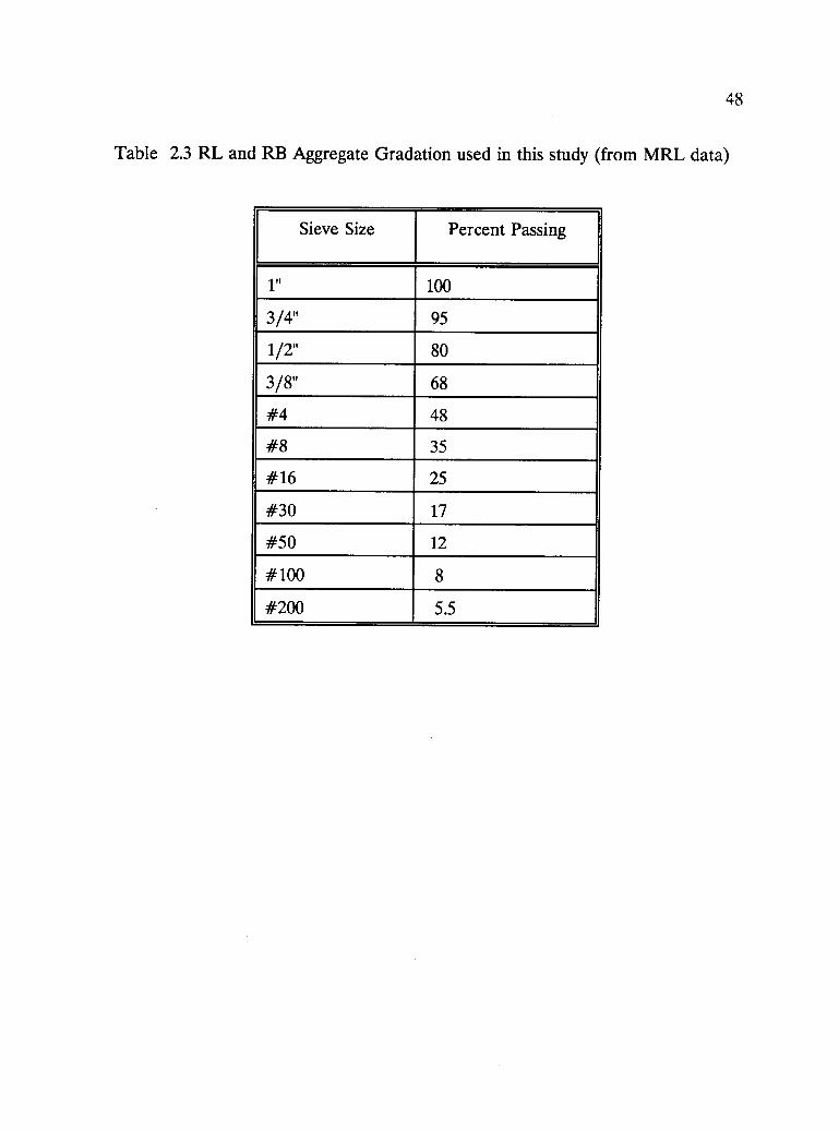
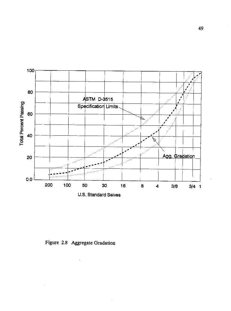
Watsonville granite (RB) and Gulf Coast gravel (RL), the gradation shown in Table
2.3 and plotted in Figure 2.8, was used in this study. It corresponds to a typical
47
Table 2.2 Mix Design Results and Compaction Efforts
Agg.Type
Asph.Type
PercentAsph. byWeight of
Agg.Compaction Effort on
Each Lift
% AirVoidsTarget
RB AAK-1 5.1 20 blows @ 300 psi and 4150 blows @ 450 psi
20 @ 150 and 8150 @ 150
AAG-1 4.9 20 @ 300 and 4150 @ 450
20 @ 175 and 8150 @ 150
RL AAK-1 4.3 20 @ 300 and 4150 @ 450
20 @ 150 and 8150 @ 150
AAG-1 4.1 20 @ 300 and 4150 @ 450
20 @ 150 and 8150 @ 150
48
Table 2.3 RL and RB Aggregate Gradation used in this study (from MRL data)
Sieve Size Percent Passing
1" 100
3/4" 95
1/2" 80
3/8" 68
#4 48
#8 35
#16 25
#30 17
#50 12
#100 8
#200 5.5
4411141"o.
-'81
20 4411P1111111:0111
St3°Seivares1°,0111111:farciall:
811,1113/8
Figure 2.8 Aggregate Gradation
3/4
49

50
dense-graded aggregate with 3/4-inch maximum size.
The two sources of asphalt differing in both composition and temperature
susceptibility (low, high) and two levels of asphalt content were used.
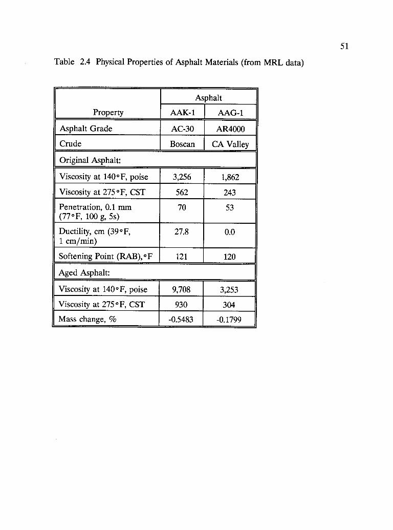
Table 2.4 shows the physical and chemical properties of each asphalt. The types of
aggregate differ in stripping potential, as known from their history of moisture
sensitivity the are low and high. Table 2.5 shows the physical and chemical properties
of each aggregate. For each asphalt-aggregate mixture, there are two levels of
compaction effort, which were established to satisfy the two levels of air voids targets.
Table 2.2 shows the compaction effort used to fabricate each asphalt-aggregate
mixture.
51
Table 2.4 Physical Properties of Asphalt Materials (from MRL data)
Property
Asphalt
AAK-1 AAG-1
Asphalt Grade AC-30 AR4000
Crude Boscan CA Valley
Original Asphalt:
Viscosity at 140°F, poise 3,256 1,862
Viscosity at 275°F, CST 562 243
Penetration, 0.1 mm(77°F, 100 g, 5s)
70 53
Ductility, cm (39°F,1 cm/min)
27.8 0.0
Softening Point (RAB),°F 121 120
Aged Asphalt:
Viscosity at 140°F, poise 9,708 3,253
Viscosity at 275°F, CST 930 304
Mass change, % -0.5483 -0.1799
52
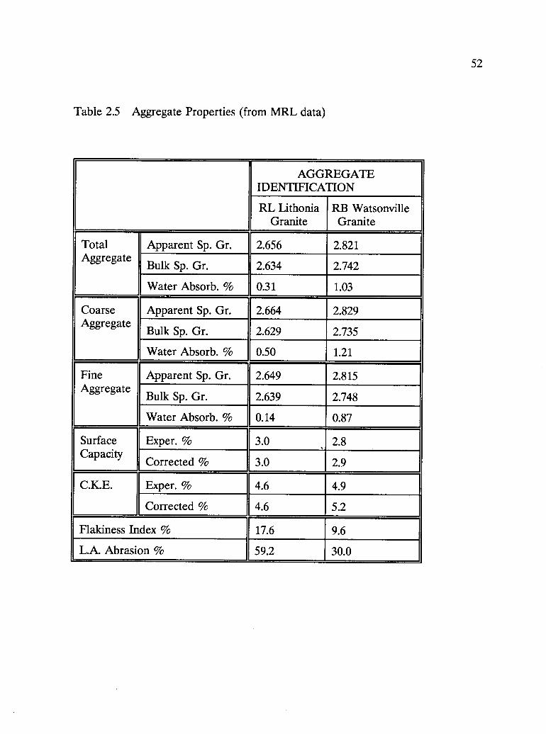
Table 2.5 Aggregate Properties (from MRL data)
AGGREGATEIDENTIFICATION
RL LithoniaGranite
RB WatsonvilleGranite
TotalAggregate
Apparent Sp. Gr. 2.656 2.821
Bulk Sp. Gr. 2.634 2.742
Water Absorb. % 0.31 1.03
CoarseAggregate
Apparent Sp. Gr. 2.664 2.829
Bulk Sp. Gr. 2.629 2.735
Water Absorb. % 0.50 1.21
FineAggregate
Apparent Sp. Gr. 2.649 2.815
Bulk Sp. Gr. 2.639 2.748
Water Absorb. % 0.14 0.87
SurfaceCapacity
Exper. % 3.0 2.8
Corrected % 3.0 2.9
C.K.E. Exper. % 4.6 4.9
Corrected % 4.6 5.2
Flakiness Index % 17.6 9.6
L.A. Abrasion % 59.2 30.0
3. TEST RESULTS
3.1 AASHTO T-283
53
A modified version of AASHTO T-283 (often called modified Lottman) was used for
predicting water damage as a basis or benchmark for comparison to the existing
procedures and current practice. The conditioning phase includes partial saturation
at 20 in. Hg vacuum for 30 minutes, followed by 15 hours freezing at -18 ° C (-0.4 °
F), 24 hours at 60° C (140 ° F) and finally 2 hours at 25 ° C (77 ° F) prior to testing
(see Appendix E for testing protocol). Evaluation includes measurement of both
resilient modulus (MR) and tensile strength (St) and reporting their retained ratios.
Additional testing was also conducted during the AASHTO T-283 procedure that will
become part of the data base. Permeability of each dry specimen was measured
using air (testing device is described in Appendix E). For those specimens which
would be water conditioned, thickness and any accompanying change in volume
(swell or shrinkage) were noted and volume calculations are shown in Table 3.1 .
An example of test data for six specimens (three for dry set and another three for
conditioning wet) is shown in Table 3.1. All data tables are in Appendix E.
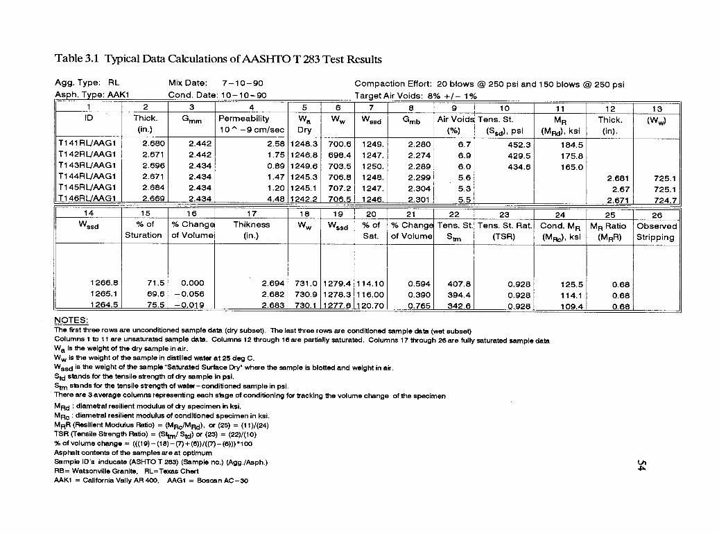
Table 3.1 Typical Data Calculations of AASHTO T 283 Test Results
Agg. Type: RLAs h. Tvi e: AAK1
Mix Date: 7-10-90Cond. Date: 10-10-90
Compaction Effort: 20 blows @ 250 psi and 150 blows @ 250 psiTarget Air Voids: 8% +/- 1%
1 2 3 4 5 6 7 8 9 10 11 12 13ID Thick. Gmm Permeability Wa Ww Wssd Gmb Air Voids Tens. St. MR Thick. (Ww)
(in.) 10 ^ -9 cm/sec Dry (%) (Ssd), psi (MRd), ksi (in).
T141RL/AAG1 2.680 2.442 2.58 1248.3 700.6 1249. 2.280 6.7 452.3 184.5T142RLJAAG1 2,671 2.442 1.75 1246.8 698.4 1247. 2.274 6.9 429.5 175.8T143RL/1AAG1 2.696 2.434 0.89 1249.6 703.5 1250. 2.289 6.0 434.6 165.0T144RL/AAG1 2.671 2.434 1.47 1245.3 706.8 1248. 2.299 5.6 2.681 725.1T145RL/AAG1 2.684 2.434 1.20 1245.1 707.2 1247. 2.304 5.3 2.67 725.1T146RL/AAG1 2.669 2.434 4.48 1242.2 706.5 1246. 2.301 5.5 2.671 724.7
14 15 16 17 18 19 20 21 22 23 24 25 26Wssd % of % Change Thikness Ww Wssd % of % Change Tens. St. Tens. St. Rat. Cond. MR MR Ratio Observed
Sturation of Volume (in.) Sat. of Volume Stm (TSR) (MRd), ksi (MRR) Stripping
1266.8 71.5 0.000 2.694 731.0 1279.4 114.10 0.594 407.8 0.928 125.5 0.681265.1 69.6 -0.056 2.682 730.9 1278.3 116.00 0.390 394.4 0.928 114.1 0.681264.5 75.5 -0.019 2.683 730.1 1277.6 120.70 0.765 342.6 0.928 109.4 0.68
NOTES:The first three rows are unconditioned sample data (dry subset). The last three rows are conditioned sample data (wet subset)Columns 1 to 11 are unsaturated sample data. Columns 12 through 16 are partially saturated. Columns 17 through 26 are fully saturated sample dataWa is the weight of the dry sample in air.Ww is the weight of the sample in distilled water at 25 deg C.Wssd is the weight of the sample "Saturated Surface Dry" where the sample is blotted and weight in air.Std stands for the tensile strength of dry sample in psi.Stm stands for the tensile strength of water-conditioned sample in psi.There are 3 average columns representing each stage of conditioning for tracking the volume change of the specimenMRd : diametral resilient modulus of dry specimen in ksi.MRa : diametral resilient modulus of conditioned specimen in ksi.MRR (Resilient Modulus Ratio) = (MRa/MRd), or (25) = (11)/(24)TSR (Tensile Strength Ratio) = (Sttm/ Std) or (23) = (22)/(10)% of volume change = (((19)- (18)- (7)+(6))/((7)- (6)))*100Asphalt contents of the samples are at optimumSample ID's inducate (ASHTO T 283) (Sample no.) (Agg./Asph.)RB= Watsonville Granite, RL=Texas CheriAAK1 = California Vally AR 400, AAG1 = Boscan AC-30
55
A summary of data for the four asphalt-aggregate combinations is shown in Table
3.2. This summary includes all the test results necessary to evaluate the effect of
water damage on the two asphalts (AAK-1 and AAG-1) and the two aggregates (RL
and RB). Visual observation for stripping rate was made after the tensile strength
test by pulling apart the two halves of the specimen at the crack. Stripping was
reported according to a modified visual evaluation rating pattern with six ranges of
stripping percentages, 5, 10, 20, 30, 40, and 50 (the method of stripping rate
evaluation is explained later).
3.2 Development of Test Methods
The intent of this section is to describe the development and evaluation of the
Environmental Conditioning System (ECS). Generally, prior to embarking on a full-
scale test scheme, numerous questions and details needed to be evaluated in
developing a testing device. Likewise, prior to starting the ECS experiment plan
(Figure 2.1) at Oregon State University, the ECS was subjected to detailed evaluation
and refinement to demonstrate its reliability and reproducibility in three aspects:
resilient modulus measurement, permeability measurement, and methods of air voids
calculations. These are discussed in the following sections.
Resilient Modulus Test
Many test procedures and types of test equipment have been developed and used in
several laboratories and-agencies to evaluate the structural properties of the asphalt
concrete mixtures. The resilient modulus of compacted asphalt mixtures can be obtained
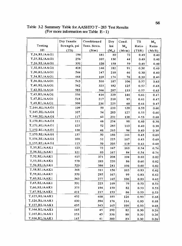
56Table 3.2 Summary Table for AASHTO T-283 Test Results
(For more information see Table E-1)
TestingID
Dry TensileStrength, psi
(TS)
ConditionedTens. Stren.
(Stm)
Dryksi
(MR)
Cond.
MR(Mrm)
TSRatio(TSR)
MRRatio
(MrR)T,24,RL/AAG1 194 181 80 72 0.49 0.40T,25,RL/AAG1 256 107 130 44 0.49 0.40T,26,RL/AAG1 331 120 158 59 0.49 0.40T,32,RL/AAG1 428 146 182 91 0.30 0.40T,30,RL/AAG1 544 147 210 66 0.30 0.40T,34,RL/AAG1 464 168 174 76 0.30 0.40T,36,RL/AAG1 543 316 187 106 0.57 0.63T,40,RL/AAG1 542 325 182 125 0.57 0.63T,42,RL/AAG1 583 366 207 133 0.57 0.63T,45,RL/AAG1 556 414 229 146 0.61 0.47T,47,RL/AAG1 518 217 210 95 0.61 0.47T,49,RL/AAG1 509 236 225 68 0.61 0.47T,144,RL/AAG1 109 59 210 120 0.53 0.60T,145,RL/AAG1 107 54 203 127 0.53 0.60T,146,RL/AAG1 117 62 231 138 0.53 0.60T,150,RL/AAG1 111 46 254 98 0.40 0.38T,151,RL/AAG1 125 52 285 113 0.40 0.38T,152,RL/AAG1 120 46 265 96 0.40 0.38T,153,RL/AAG1 137 50 186 141 0.43 0.69T,154,RL/AAG1 100 52 225 167 0.43 0.69T,155,RL/AAG1 113 50 205 119 0.43 0.69T,35,RL/AAK1 123 72 167 163 0.54 0.74T,38,RL/AAK1 121 60 167 84 0.54 0.74T,52,RL/AAK1 415 371 208 104 0.60 0.82T,53,RL/AAK1 570 283 220 86 0.60 0.82T,56,RL/AAK1 520 386 241 106 0.60 0.82T,58,RL/AAK1 368 311 156 105 0.83 0.62T,59,RL/AAK1 370 295 167 99 0.83 0.62T,60,RL/AAK1 363 277 165 106 0.83 0.62T,65,RL/AAK1 331 223 169 79 0.53 0.53T,66,RL/AAK1 375 194 159 82 0.53 0.53T,67,RL/AAK1 411 217 153 86 0.53 0.53
T,125,RL/AAK1 452 408 185 126 0.93 0.68T,126,RL/AAK1 430 394 176 114 0.93 0.68T,127,RL/AAK1 435 343 165 109 0.93 0.68T,164,RL/AAK1 145 45 292 82 0.30 0.26T,165,RL/AAK1 153 45 336 80 0.30 0.26T,166,RL/AAK1 145 41 300 83 0.30 0.26
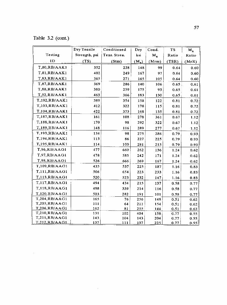
57
Table 3.2 (cont.)
TestingID
Dry TensileStrength, psi
(TS)
ConditionedTens. Stren.
(Stm)
Dryksi
(MR)
Cond.
MR
(Mrm)
TSRatio
(TSR)
MRRatio(MrR)
T,80,RB/AAK1 352 238 148 99 0.64 0.60T,81,RB/AAK1 402 249 167 97 0.64 0.60T,83,RB/AAK1 365 271 165 105 0.64 0.60T,87,RB/AAK1 369 286 140 106 0.65 0.61T,88,RB/AAK1 380 259 175 93 0.65 0.61T,92,RB/AAK1 463 366 183 130 0.65 0.61
T,102,RB/AAK1 389 354 158 122 0.81 0.72T,103,RB/AAK1 412 322 178 115 0.81 0.72T,104,RB/AAK1 422 373 168 135 0.81 0.72T,187,RB/AAK1 161 108 278 361 0.67 1.12T,188,RB/AAK1 170 98 292 322 0.67 1.12T,189,RB/AAK1 148 116 289 277 0.67 1.12T,193,RB/AAK1 134 98 275 286 0.79 0.93T,194,RB/AAK1 113 86 227 225 0.79 0.93T,195,RB/AAK1 114 100 281 215 0.79 0.93T,96,RB/AAG1 477 660 262 136 1.24 0.62T,97,RB/AAG1 478 585 242 171 1.24 0.62T,98,RB/AAG1 526 666 269 167 1.24 0.62T,109,RB/AAG1 435 537 225 187 1.16 0.83T,111,RB/AAG1 506 654 223 233 1.16 0.83T,113,RB/AAG1 520 523 232 147 1.16 0.83T,117,RB/AAG1 494 434 215 137 0.58 0.77T,118,RB/AAG1 498 339 214 116 0.58 0.77T,120,RB/AAG1 503 282 191 101 0.58 0.77T,204,RB/AAG1 165 76 256 148 0.51 0.62T,205,RB/AAG1 111 64 211 154 0.51 0.62T,206,RB/AAG1 162 81 255 144 0.51 0.62T,210,RB/AAG1 131 102 404 158 0.77 0.55T,211,RB/AAG1 143 104 143 204 0.77 0.55T,212.RB/AAG1 137 111 137 225 0.77 0.55
58
by using either repeated loading triaxial test or repeated loading indirect tensile test
(Al- Swailmi et al., 1992). These two test procedures have been standardized by
ASTM as: (1) the Standard Test Method for Dynamic Modulus of Asphalt Mixtures,
(ASTM D 3497) and (2) the Standard Method of Indirect Tension Test for Resilient
Modulus of Bituminous Mixtures (ASTM D 4123). Unfortunately, these procedures
do not always yield similar results.
In the ECS, the resilient modulus is defined as the ratio of the applied axial stress
to the corresponding recoverable (elastic) axial strain. The vertical stress is applied
axially by using an electro-pneumatic closed loop testing system. Applied stress is
controlled by a load cell placed on the top of the specimen. Recoverable axial strain
is monitored by LVDTs. Stresses and strains are recorded and analyzed by the
computer and software package.
For axial loading, the appropriate specimen height as recommended in ASTM
D 3497 should be at least 8-in. for a 4-in. diameter specimen. However, it was not
feasible to water condition these tall specimens, because of the long distance for the
water to flow under vacuum. To compromise between the ASTM D 3497
requirement and typical pavement layer thicknesses, a mini-study was conducted to
investigate the effect of height-to-diameter (L/D) ratio, on resilient modulus. In
addition, other mini-studies were conducted to investigate other details including:
1) Effect of glue type for strain gages (strain gages were later replaced by
LVDTs)
59
2) Repeatability of ECS resilient modulus and necessity of using teflon
disks.
Test Specimen Preparation
One mix, combination RB/AAK-1, was used to prepare three 4-in. diameter by 7 in.
high specimens. After density determinations were completed, a vertical alignment
jig was used with capping compound to maintain caps perpendicular with the
specimen axis according to the requirements of ASTM C 617, "Capping Cylindrical
Concrete Specimens". After testing the specimens with the full height, 1.0 in. was
trimmed from each end with a diamond saw. Capping and testing were repeated for
the new 5-in. specimen. Finally, 1.25 in. were trimmed from each end of the 5-inch
specimen which resulted in 2.5 in. specimens and exposed to the same capping and
testing procedure. Trimmed specimen densities and air void calculations were
monitored for the three heights as shown in Table 3.3.
Test Equipment and Instrumentation
In this mini-study, an MTS electro-hydraulic closed-loop system was used for the
dynamic compression loading and stresses were monitored by chart recorder.
Recoverable axial strain was measured by two techniques:

60
Table 3.3 Density and Air Void Calculations for the Three Specimen Thicknesses
SpecimenID
OriginalThickness(- 7" thickness)
After first cut(- 5" thickness)
After second cut(- 2.5" thickness)
Bulkspec.gravity
%AirVoids
Bulkspec.gravity
%AirVoids
Bulk spec.gravity
%AirVoids
RB/AAK1-1 2.245 8.5 2.255 8.1 2.248 8.4
RB/AAK1-2 2.255 8.1 2.241 8.7 2.218 9.6
RB/AAK1-3 2.255 8.1 2.245 8.5 2.238 8.8
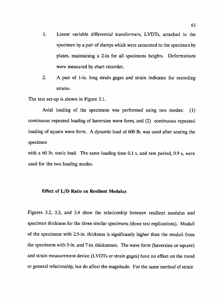
61
1. Linear variable differential transformers, LVDTs, attached to the
specimen by a pair of clamps which were cemented to the specimen by
plates, maintaining a 2-in for all specimens heights. Deformations
were measured by chart recorder.
2. A pair of 1-in. long strain gages and strain indicator for recording
strains.
The test set-up is shown in Figure 3.1.
Axial loading of the specimens was performed using two modes: (1)
continuous repeated loading of haversine wave form, and (2) continuous repeated
loading of square wave form. A dynamic load of 600 lb. was used after seating the
specimen
with a 60 lb. static load. The same loading time 0.1 s, and rest period, 0.9 s, were
used for the two loading modes.
Effect of L/D Ratio on Resilient Modulus
Figures 3.2, 3.3, and 3.4 show the relationship between resilient modulus and
specimen thickness for the three similar specimens (three test replications). Moduli
of the specimens with 2.5-in. thickness is significantly higher than the moduli from
the specimens with 5-in. and 7-in. thicknesses. The wave form (haversine or square)
and strain measurement device (LVDTs or strain gages) have no effect on the trend
or general relationship, but do affect the magnitude. For the same method of strain
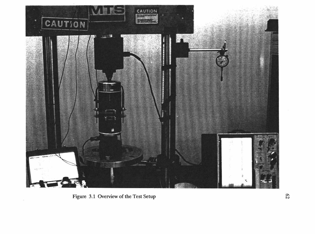
Figure 3.1 Overview of the Test Setup
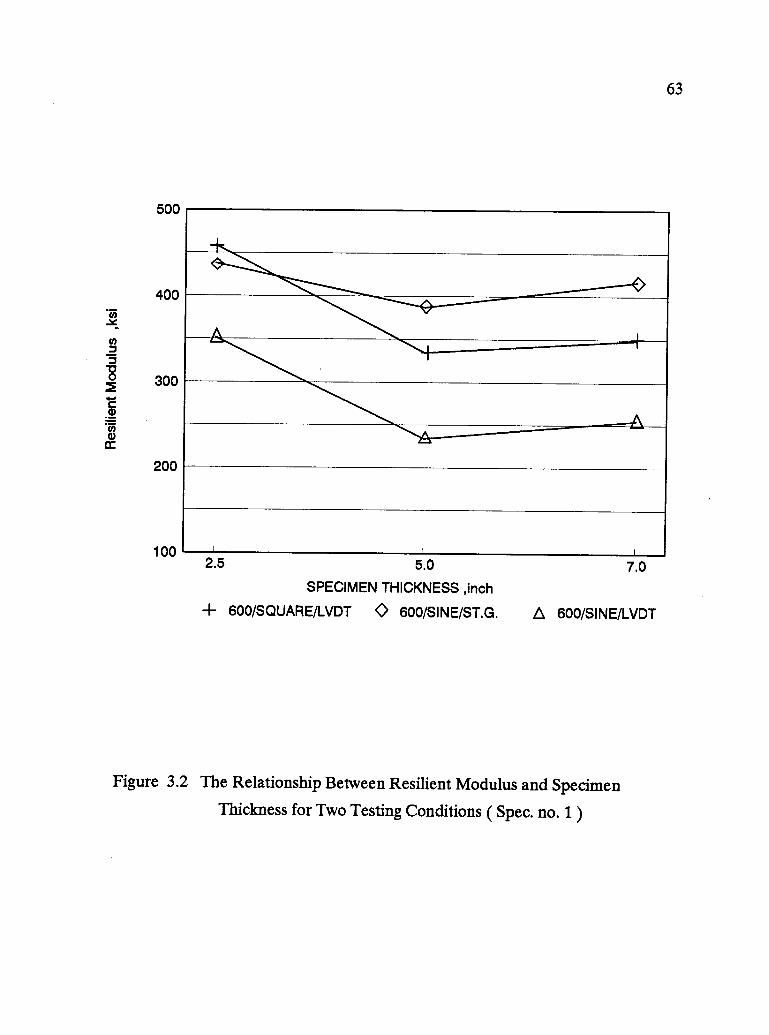
500
400
300
200
100
63
2.5 5.0 7.0
SPECIMEN THICKNESS ,inch
--I- 600/SQUARE/LVDT 0 600/SINE/ST.G. A 600/SINE/LVDT
Figure 3.2 The Relationship Between Resilient Modulus and Specimen
Thickness for Two Testing Conditions ( Spec. no. 1)
1200
1000
800
600
400
200
-11
-IA
2.5 5.0
SPECIMEN THICKNESS ,inch
600/SQUARE/ST.G. + 600/SQUARE/LVDT .0. 600/SINE/ST.G. A 600/SINE/LVDT
7.0
64
Figure 3.3 The Relationship Between Resilient Modulus and Specimen
Thickness for Two Testing Conditions ( Spec. no. 2 )
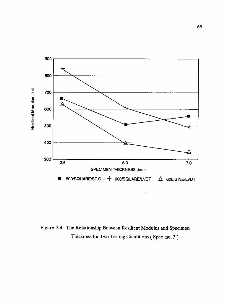
900
800
700
600
500
400
300
65
,
2.5 5.0
SPECIMEN THICKNESS ,inch
7.0
600/SQUARE/ST.G. + 600/SQUARE/LVDT A 600/SINE/LVDT
Figure 3.4 The Relationship Between Resilient Modulus and Specimen
Thickness for Two Testing Conditions ( Spec. no. 3 )
66
measurement and load level, the MR from the square wave mode is higher than the
MR from the haversine wave form, as shown in Figures 3.2, 3.3, and 3.4.
For the same wave form, strain gages detect less strain, which resulted in a higher
MR than with the LVDTs. Strain gages may not indicate the total strain as the
LVDTs do because large stones located behind the strain gages may not transmit the
total strain. In contrast, LVDTs measure the cumulative strain between two points,
which may be more realistic. In addition, during the ECS testing program it has
been noticed that the strain gages mounted on specimens with high air voids (such
as 10%) experienced major wrinkles under the effect of repeated loading with hot
water conditioning. The deformed strain gages were most likely caused by large total
deformation due to compaction or densification. Because of such deficiencies
associated with the strain gages and due to their cost, a decision was made to switch
to LVDTs after a significant part of the ECS testing program was completed using
strain gages, particularly the low air void specimens.
Finally, from the above investigation, it was concluded that the specimen thickness
has considerable effect on resilient modulus value and the specimen closest in
thickness to 8-in. (L/D = 2.0) gives the closest to "true" resilient modulus. For the
ECS, it is sufficient to monitor relative change in resilient modulus during water
conditioning which indicates the real MR change. This concept of relative MR using
a 4-in. specimen has been used as a compromise for an 8-in. specimen (4-in.
specimens are easier to produce and test and are more representative of actual
67
pavement lift thicknesses). Thus, a 4-in. high specimen was recommended and is
used for the ECS testing.
Since the resilient modulus value from the ECS is not the true or familiar MR, the
term "ECS-MR" will be used in this paper for 4-in. specimens. Therefore, there are
two important differences between the ECS-MR and the dynamic modulus defined
in ASTM D 3497: 1) the height of the specimen is 4 in. instead of 8 in., and 2) the
specimen is encapsulated in a rubber membrane throughout the test. In addition to
"ECS-MR," a diametral MR is measured for each specimen prior to the ECS
procedure, to be used for reporting the initial specimen stiffness. All values of MR
in this report stand for "ECS-MR" unless otherwise noted.
Effect of Strain Gage Glue Type
Six strain gages: Xi, X2, X3, Ylf Y2, and Y3, were bonded on a 7.5 in. high by 4 in. in
diameter plastic specimen. The strain gages were divided into two groups and each
group was mounted at mid-height and opposite to the other group. The two groups
are: (1) X1, X2, and X3 were bonded on side X; and (2) Yi, Y2, and Y3 were bonded
on side Y. Three different glue types were used for bonding the strain gages with
to the following identification:
X, and Yi: 1 inch strain gage with "super glue"
X2 and Y2: 1 inch strain gage with Ca-200LS glue
X3 and Y3: 1 inch strain gage with Testors "airplane" glue
68
Specimens were subjected to dynamic repeated loading by using the MTS and strains
were monitored by strain indicator. Figure 3.5 shows resilient modulus results from
each strain gage. The difference among glue types is not significant. The MR on side
X was higher than on side Y due to eccentricity but was later corrected. As a result
of this experiment, super glue was selected for future strain gage application because
it needs very short time to cure.
Repeatability of ECS-MR and Effect of Teflon Disks
Six specimens were used to investigate the repeatability of the ECS-MR, and the
effect of friction between the specimen and the top cap and bottom base. It was
suggested that teflon disks help in reducing the friction between the specimen and
the top cap and bottom base. The following specimens were used in the study:
1) 1 PLAS and 2 PLAS:
2) 54TB and 62TB:
3) TG61 and WG77:
4 inches in diameter by 2.5 inches in
height, plastic specimen
4 inches in diameter by 2.5 inches in
height, asphalt concrete specimen
4 inches in diameter by 4 inches in height,
asphalt concrete specimen

290
280
270
260
250
240
230
220
210
69
X1 X2 X3 Y1
STRAIN GAGE TYPE
Y2
Figure 3.5 Effect of Strain Gage Mounting Glue on Resilient Modulus
Y3
70
Strain gages 1 in. long were used on 2.5 in. high specimens, and 2 in. strain gages
were used on the 4 in. specimens. The ECS was used to conduct resilient modulus
tests. Two types of 1/8 in. thick teflon disk were used: solid and perforated.
Table 3.4 shows test results of tests performed on each specimen according to the
following combinations:
1) No disks: No disks were used
2) One disk: One solid teflon disk top and bottom
3) Perf. disk: One perforated teflon disk top and bottom
4) Two disks: Two solid teflon disks top and bottom
5) One disk: One solid teflon disk top and bottom
6) Diff. Or: One solid disk top and bottom with different orientation
by rotating the specimens 180° around its vertical axis.
The test of the one disk setting was repeated twice to show the repeatability of
ECS-MR for the test setting which represents the ECS testing program standard.
Figure 3.6 shows the plots of ECS-MR for all test settings from each specimen. For
all six specimens, the repeatability of one disk setting is very high. Teflon disk and
test orientation does not affect the results for the plastic specimen because of the
frictionless surfaces and high uniformity of this material. Teflon disks and test
orientation has a significant effect on ECS-MR of 2.5 inch asphalt concrete specimens,
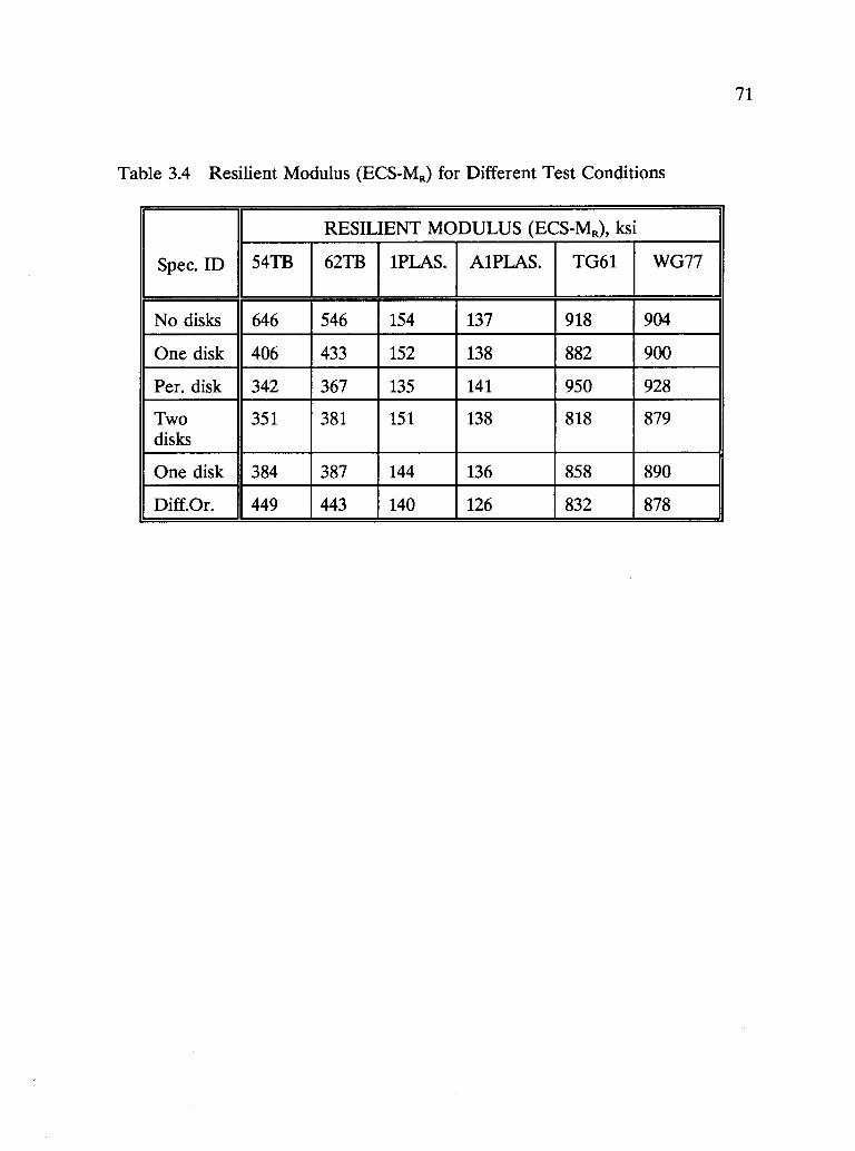
71
Table 3.4 Resilient Modulus (ECS-MR) for Different Test Conditions
Spec. ID
RESILIENT MODULUS (ECS-MR), ksi
54TH 62TB 1PLAS. AlPLAS. TG61 WG77
No disks 646 546 154 137 918 904
One disk 406 433 152 138 882 900
Per. disk 342 367 135 141 950 928
Twodisks
351 381 151 138 818 879
One disk 384 387 144 136 858 890
Diff.Or. 449 443 140 126 832 878
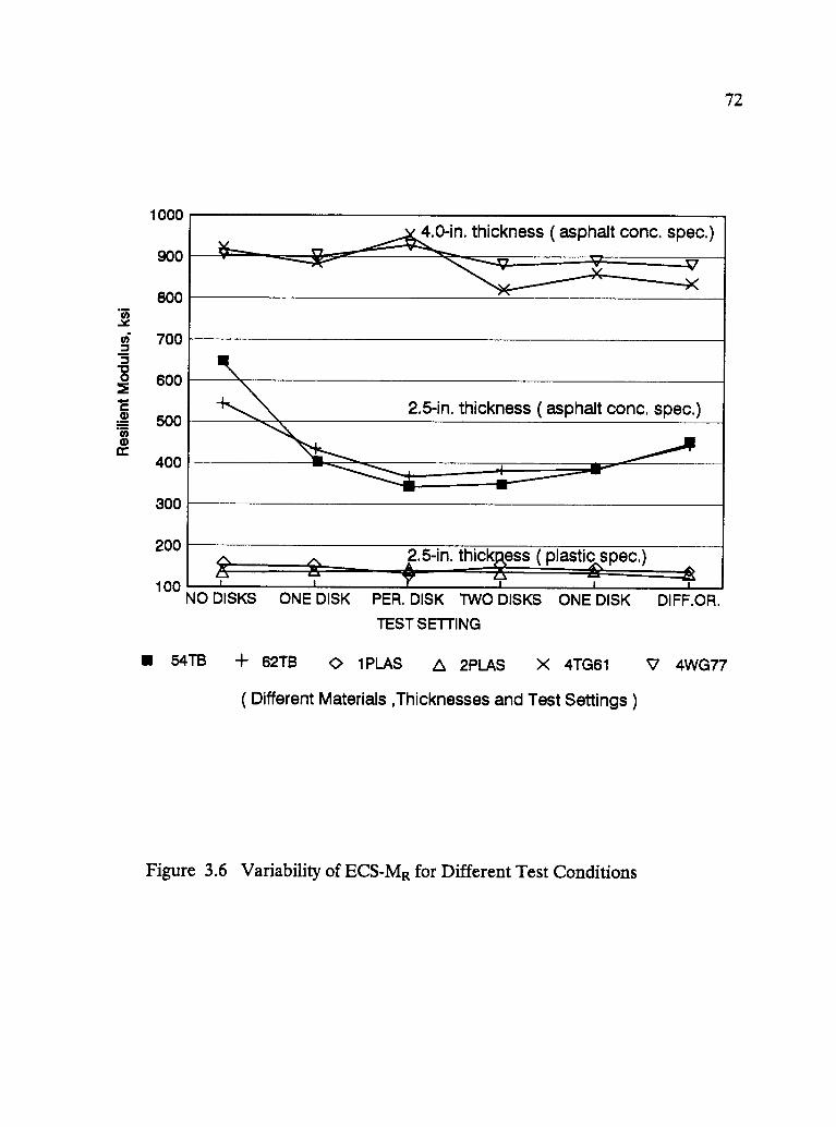
1000
900
800
700
600
500
400
300
200
72
4.0-in. thickness ( asphalt conc. spec.)
V
2.5-in. thickness ( asphalt conc. spec.)
100 'NO DISKS ONE DISK PER. DISK TWO DISKS ONE DISK DIFF.OR.
TEST SETTING
54TB 62TB O 1PLAS A 2PLAS X 4TG61 V 4WG77
( Different Materials ,Thicknesses and Test Settings )
2.5-in. thickBess (plastics spec.)
Figure 3.6 Variability of ECS-MR for Different Test Conditions

73
54TB and 62TB. The effect of teflon disks and test orientation on ECS-MR from
4 inch asphalt concrete specimens is not significant.
It was found necessary to use perforated spacers between the specimen and top cap
and base plate to collect any stripped asphalt which may stick on the bottom of the
top cap during the water conditioning process and change its serviceability condition,
also to permit water to pass through. Perforated teflon disk top and bottom are
recommended to be used with the ECS testing program. Perforation pattern, hole
diameter, and groove pattern for base and top cap are shown in Figure 3.7.
Permeability Measurements
Permeability (K) by definition, Goode and Lufsey 1965, is the volume of fluid, Q, of
unit viscosity, it, passing in unit time, At, through a unit cross section, A, of a porous
medium of length, L, under the influence of a unit pressure gradient, AP.
K-AAP At
There is a general belief that permeability is a better measure of durability than
percent air voids because permeability measures fluid accessibility through the
asphalt pavement. Percent air voids may include voids not accessible by water. In
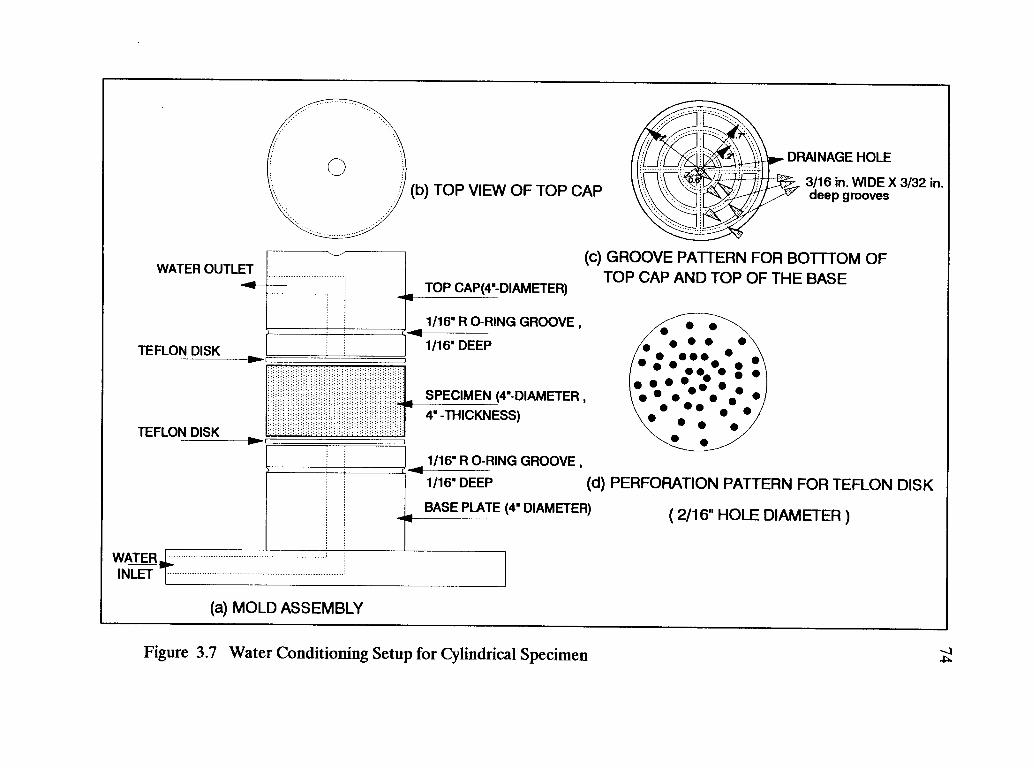
WATER OUTLET
TEFLON DISK
(b) TOP VIEW OF TOP CAP
DRAINAGE HOLE
3/16 in. WIDE X 3/32 in.deep grooves
(c) GROOVE PATTERN FOR BOTTTOM OFTOP CAP AND TOP OF THE BASE
TOP CAP(4'- DIAMETER)
1/16' R 0-RING GROOVE ,
1/16' DEEP
SPECIMEN (4'-DIAMETER ,044' -THICKNESS)
TEFLON DISK
WATERINLET
f;
1/16' R 0-RING GROOVE ,
1/16' DEEP (d) PERFORATION PATTERN FOR TEFLON DISK
BASE PLATE (4' DIAMETER) ( 2/16" HOLE DIAMETER )
(a) MOLD ASSEMBLY
Figure 3.7 Water Conditioning Setup for Cylindrical Specimen

75
the ECS testing program, a relationship was hypothesized between permeability and
water damage.
Based on the above introduction, it was necessary to conduct several mini-studies to
investigate factors related either to permeability testing technique or the role of
permeability in the testing program. The topics covered by these mini-studies are as
follows:
1. Effect of specimen surface flow control on permeability.
2. Effect of compaction procedure on specimen surface sealing.
3. Differential pressure level-permeability relationship.
4. Permeability as a measure of specimen volume change.
5. Specimen internal coloring indicator.
Effect of Specimen Surface Flow on Permeability
In order for the air flow to pass only through the specimen during the permeability
test, the outer surface of the specimen wall must be sealed. Goode and Lufsey
(1965) used paraffin for sealing to prevent leakage between the specimen wall and
the membrane. However, this method destroys the specimen for further use by
contaminating the asphalt.
76
Another method is to place the specimen in a cylindrical rubber membrane fastened
to a hollow metal cylinder with hose clamps. This method does not totally prevent
leakage between the specimen wall and the membrane, especially with coarse
mixtures. Another disadvantage of this method is that deformation of the specimen
may be caused by the air pressure in the membrane.
Kumar and Goetz (1977) developed a different technique to prevent leakage. The
specimen is placed between two collars (lower collar and upper collar) and coated
with silicone rubber sealer all around the specimen and part of both collars in order
to bind the collars to the specimen. This method prevented the leakage along the
specimen wall, but it is rather involved and time consuming.
In the modified procedure developed at OSU (Al-Swailmi and Terrel) 1992,the
middle one-third of the specimen's surface is coated with silicone and then enveloped
with a cylindrical rubber membrane 1.5 in. high (a wide rubber band, cut from a
membrane) to provide a smooth surface. After curing a few hours, the specimen is
fitted with a cylindrical rubber membrane, long enough to envelope the sample base
and sample top cap. This procedure has been adopted after investigating three levels
of silicone seals on the surface of the specimen and under the rubber membrane
which showed that the "standard" procedure of a single seal at the mid-point was
adequate as shown in Figure 3.8. For additional details about the permeability
protocol, see Appendix F.
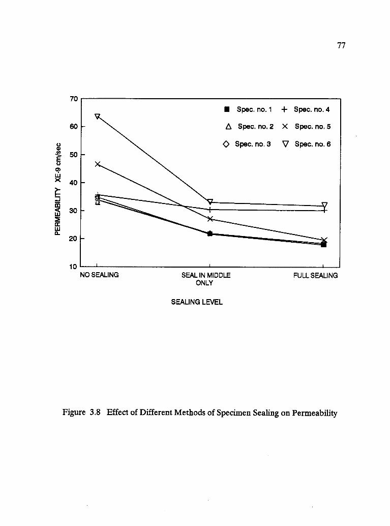
70
60
0a)
50
0)
W 40
Min6 302Qwa_
20
10
77
NO SEALING SEAL IN MIDDLEONLY
SEALING LEVEL
FULL SEALING
Figure 3.8 Effect of Different Methods of Specimen Sealing on Permeability
78
Effect of Compaction Procedure on Specimen Surface Sealing
From observation, a sealing effect on the end surface specimen during compaction
(kneading) was of some concern. Since this effect was expected, several trials were
conducted by sawing the specimen ends to obtain a "true" permeability value. Both
wet sawing and dry sawing were used. Table 3.5 shows a summary of permeability
measurements comparing as-molded briquets and briquets with 1/4 in. sawed off
each end (dry and wet sawing). Dry sawing at ambient temperature shows a 40%
decrease in permeability compared to as-molded permeability. This unexpected
result was due to the high temperature created by the friction between the saw and
the aggregate which resulted in melting the asphalt and creation of another seal by
smearing the asphalt binder across the surface. This explanation was confirmed by
dry sawing (in a controlled temperature room) at 0°C (32°F) and applying CO, to
reduce the effect of heating during sawing. Cold dry sawing shows higher
permeability (Table 3.5) than the wet sawing; however, both wet and dry sawing at
ambient temperature resulted in lower permeability. From the above comparison, it
was concluded that cold dry sawing is appropriate for the "standard" ECS specimen
preparation, which is used for slab and field specimens.
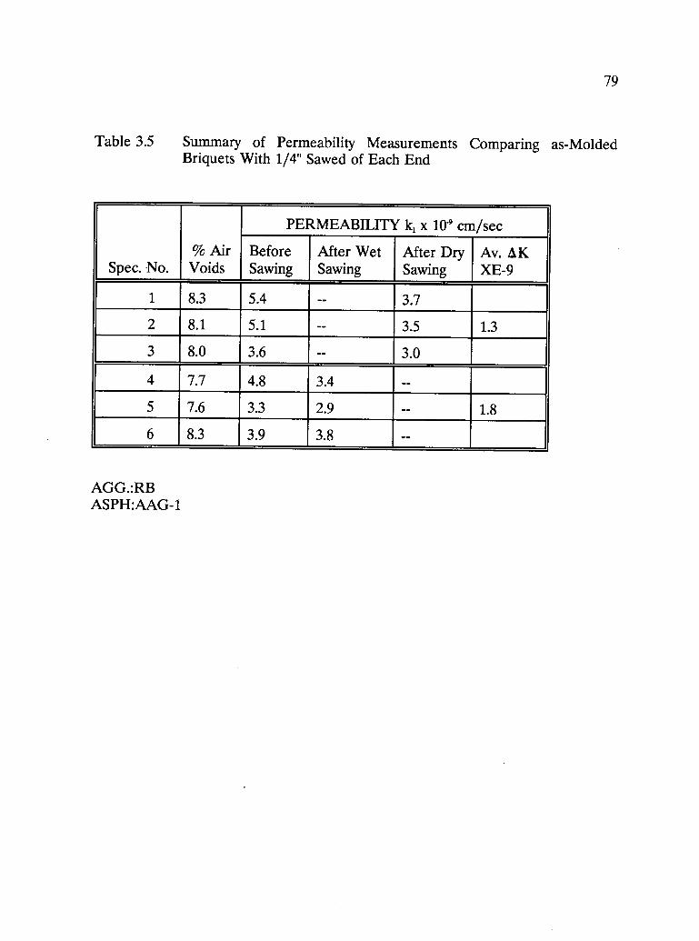
79
Table 3.5 Summary of Permeability Measurements Comparing as-MoldedBriquets With 1/4" Sawed of Each End
Spec. No.% AirVoids
PERMEABILITY k, x 10' cm/sec
BeforeSawing
After WetSawing
After DrySawing
Av. AKXE-9
1 8.3 5.4 -- 3.7
2 8.1 5.1 -- 3.5 1.3
3 8.0 3.6 -- 3.0
4 7.7 4.8 3.4 --
5 7.6 3.3 2.9 -- 1.8
6 8.3 3.9 3.8 --
AGG.:RBASPH:AAG-1
80
Differential Pressure Level- Permeability Relationship
The permeability test is not only critical to the test parameter setup as explained
earlier, but it is also critical to the test conditions. The following steady state
conditions, are required for the permeability test:
1. Continuity of flow with no volume change during a test.
2. Flow with the voids fully saturated.
3. Flow in the steady state with no changes in pressure gradient.
In order to be sure that the test was performed in a steady state condition, at least
three air flow readings for three differential pressure readings were required. The
rate of air flow "Q" versus differential pressure "AP" is plotted, and the slope, __q_ ,AP
of the straight line portion of the curve using linear regression equation is obtained
(Kummer, 1977). By using specimen thickness and this slope value, the permeability
can easily be calculated. Statistically, the degree of the variation from the straight
line can be judged from r-squared (r2) value.
81
study was conducted to investigate the relation between r2 and differential pressure
level. A permeameter, Figure 3.9, was fabricated with three levels of air flow meters
and four levels of differential pressure meters. The differential pressure meters are
as follows:
1. Differential pressure meter with a range of 2 cm of water and minor
division of 0.1 mm.
2. Differential pressure meter with a range of 5 cm of water and minor
division of 1.0 mm.
3. Water manometer with a range of 30 cm. and minor division of
1.0 mm.
4. Mercury manometer with a range of 76 cm. and minor divisions of
0.25 cm.
An open-graded asphalt concrete specimen was prepared with 20% air voids so that
a wide range of air flow rates and differential pressures could be used. Sixty-four air
flow rates and differential pressure readings were reported for a range of differential
pressure from 0.03 to 34.5 cm of water and a range of air flow rate from 110 to
18,876 cm3 /min, see Table 3.6.
Figure 3.10 shows a plot of flow rate vs. differential pressure which is divided into
five ranges according to the differential pressure meters which are indicated in
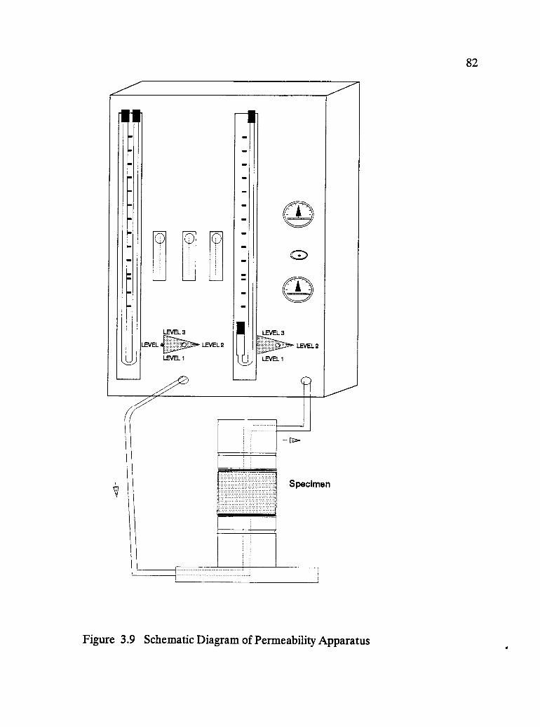
82
7
LEVEL 3
LEVEL 4
LEVEL 1
7
LEVEL 2
C)
LEVEL 3,
:,::;i::;:;::::
LEVEL 1
LEVEL 2
C
Specimen
Figure 3.9 Schematic Diagram of Permeability Apparatus
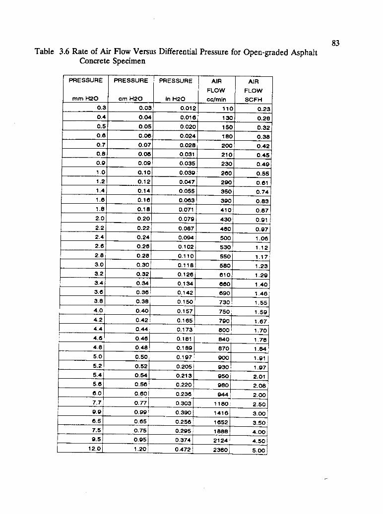
83Table 3.6 Rate of Air Flow Versus Differential Pressure for Open-graded Asphalt
Concrete Specimen
PRESSURE
mm H2O
PRESSURE
cm H2O
PRESSURE
In H2O
AIR
FLOW
cc/min
AIR
FLOW
SC FH0.3 0.03 0.012 110 0.230.4 0.04 0.016 130 0.280.5 0.05 0.020 150 0.320.8 0.06 0.024 180 0.380.7 0.07 0.028 200 0.420.8 0.08 0.031 210 0.450.9 0.09 0.035 230 0.491.0 0.10 0.039 260 0.551.2 0.12 0.047 290 0.611.4 0.14 0.055 350 0.741.8 0.16 0.063 390 0.831.8 0.18 0.071 410 0.872.0 0.20 0.079 430 0.912.2 0.22 0.087 460 0.972.4 0.24 0.094 500 1.082.6 0.28 0.102 530 1.122.8 0.28 0.110 550 1.173.0 0.30 0.118 580 1.233.2 0.32 0.126 610 1.293.4 0.34 0.134 660 1.403.6 0.36 0.142 890 1.463.8 0.38 0.150 730 1.554.0 0.40 0.157 750 1.594.2 0.42 0.165 790 1.674.4 0.44 0.173 800 1.704.6 0.46 0.181 840 1.784.8 0.48 0.189 870 1.845.0 0.50 0.197 900 1.915.2 0.52 0.205 930 1.975.4 0.54 0.213 950 2.015.8 0.56 0.220 980 2.086.0 0.60 0.236 944 2.007.7 0.77 0.303 1180 2.509.9 0.99 0.390 1416 3.006.5 0.65 0.256 1852 3.507.5 0.75 0.295 1888 4.009.5 0.95 0.374 2124 4.50
12.0 1.20 0.4721 2380 5.00
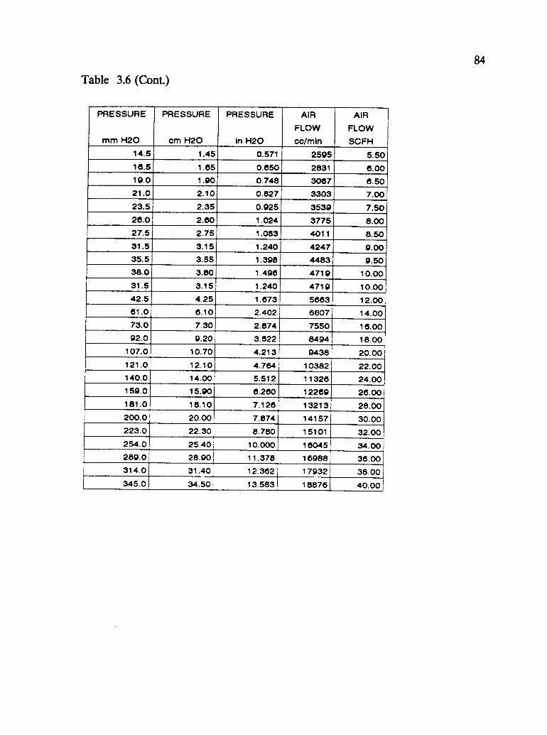
84
Table 3.6 (Cont.)
PRESSURE
mm H2O
PRESSURE
cm H2O
PRESSURE
in H2O
AIR
FLOW
cc/min
AIR
FLOW
SCFH14.5 1.45 0.571 2595 5.5016.5 1.65 0.650 2831 6.0019.0 1.90 0.748 3067 8.5021.0 2.10 0.827 3303 7.0023.5 2.35 0.925 3539 7.5026.0 2.60 1.024 3775 8.0027.5 2.75 1.083 4011 8.5031.5 3.15 1.240 4247 0.0035.5 3.55 1.398 4483 9.5038.0 3.80 1.496 4719 10.0031.5 3.15 1.240 4719 10.0042.5 4.25 1.673 5663 12.0061.0 6.10 2.402 6607 14.0073.0 7.30 2.874 7550 16.0092.0 9.20 3.622 8494 18.00
107.0 10.70 4.213 9438 20.00121.0 12.10 4.784 10382 22.00140.0 14.00 5.512 11326 24.00159.0 15.90 6.260 12260 26.00181.0 18.10 7.126 13213 28.00200.0 20.00 7.874 14157 30.00223.0 22.301 8.780 15101 32.00254.0 25.401 10.000 18045 34.00289.0 28.90 11.378 16988 36.00314.0 ,31.401 12.362 17932 38.00345.0 34.50 13.583 I 18876 40.00
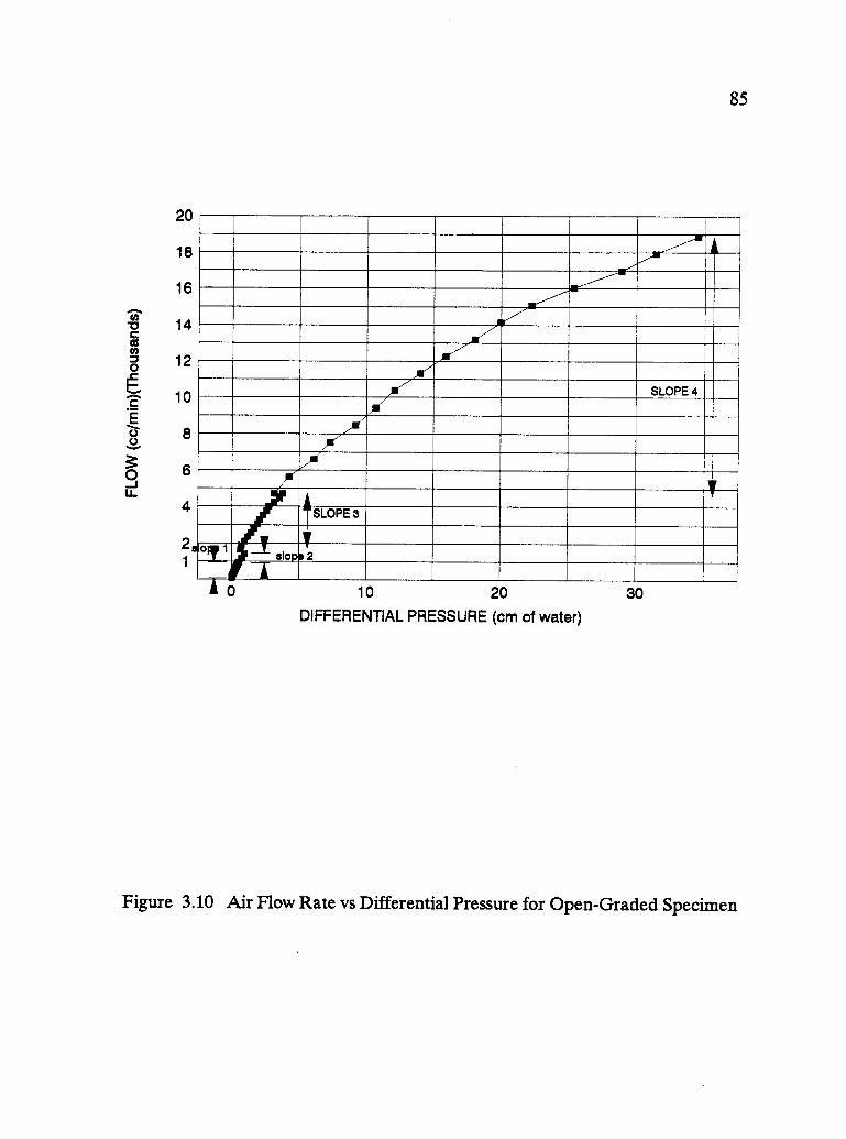
20
18
16
14
12
10
8
6
4
21
85
A
SLOPE 4
oT 1
A71elope
SLOPE 3
2
V
0 10 20
DIFFERENTIAL PRESSURE (cm of water)
30
Figure 3.10 Air Flow Rate vs Differential Pressure for Open-Graded Specimen

86
Figure 3.10 by different slopes. The discontinuity in the data (plot) is due to
changing either the flow meter or the differential pressure gage. Permeability was
calculated for each range and over the entire range as well. Table 3.7 shows
permeability "K," slope, and r2. No significant relationship exists between
permeability and r2 for two of the ranges with r2 equal 1.0. the permeabilities, K2 and
Ks, are significantly different (4.05E-08 and 2.75E-07, respectively), however.
It was concluded from this study that indicating the steady state by the slope of the
straight line portion of the curve (flow rate versus differential pressure) with a high
r2, is not the best method. On the other hand, it was found that using the lowest
differential pressure possible during the permeability test is the best method for
maintaining the steady state, because the lowest differential pressure value is the
flattest slope over a wide range of flow rate-differential pressure measurements, as
shown in Figure 3.10.
Permeability as a Measure of Specimen Volume Change
Volume change of specimen, swell or shrinkage, often occurs during water
conditioning and is important for understanding asphalt pavement behavior during
the water damage process. Specimen volume change was determined for AASHTO
T-283 specimens (see Section 3) by reporting specimen bulk specific gravity and
saturated surface dry weight for the three conditioning stages: dry, partially
saturated, and at the conclusion of water conditioning. Likewise, specimen thickness

87
Table 3.7 The Relationship Between r-squared and Permeability
SLOPE PERMEABILITY,
cm/s, (K)
r-squared
First Range 1661 5.81 E-07 0.99
Second Range 116 4.05 E-08 1.00
Third Range 976 3.42 E-07 0.99
Fourth Range 785 2.75 E-07 1.00
Fifth Range 449 1.57 E-07 0.97
Whole Range 638 2.24 E-07 0.95
88
was measured using ASTM D 3549 for the specimen for the same three conditioning
stages. Logically, any thickness increase should be combined with volume increase.
In contrast, the results show no significant relation between specimen thickness
change and specimen volume change, as shown in Figure 3.11. This means that bulk
specific gravity test is not the appropriate method for monitoring specimen volume
change during water conditioning cycles.
In the ECS testing program, specimen volume change was monitored by two
methods:
1. Monitoring specimen thickness during water conditioning by LVDT
attached to the top of the specimen and connected to a PC computer
for data acquisition.
2. Monitoring the internal voids volume changes by determining water
permeability at the end of each water conditioning cycle.
Specimen Internal Coloring Indicator
In order to investigate water accessibility to the internal air voids of asphalt concrete
specimens, dye-treated water was used to wet specimens under the effect of the ECS
standard vacuum, 20 inches of Hg. The specimens were then split open diameterally
and examined. All interior voids appeared to be dye-stained, thus water access was
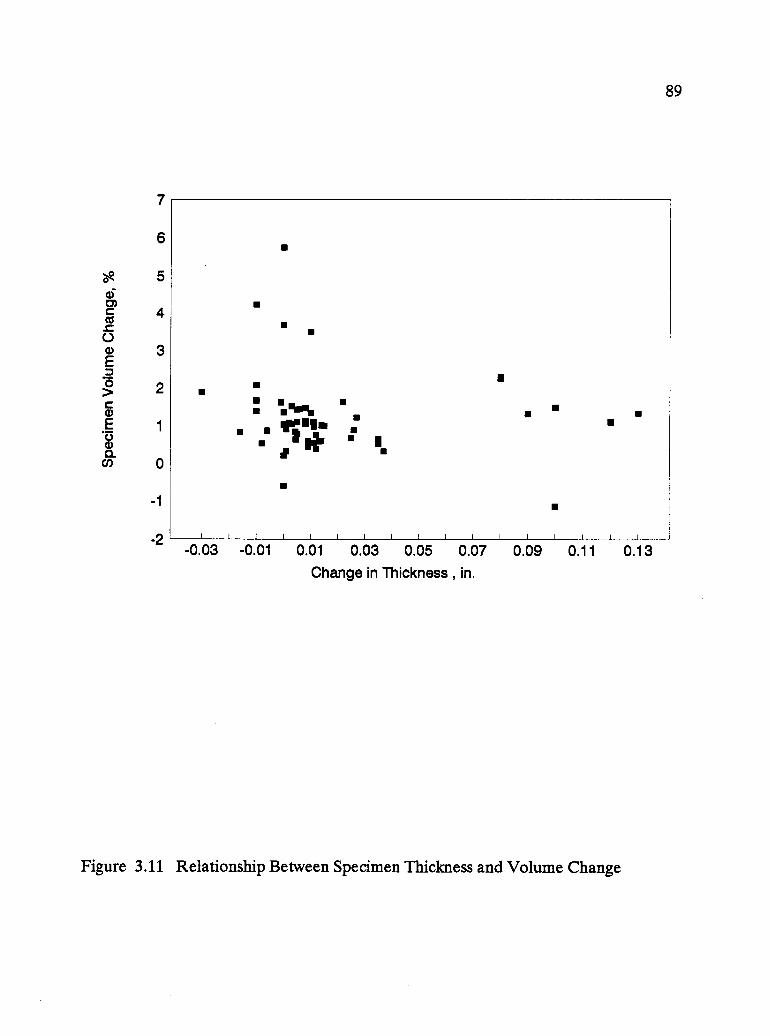
7
6
5
4
3
2
1
0
-1
-2-0.03 -0.01 0.01 0.03 0.05 0.07 0.09 0.11
Change in Thickness , in.
89
Figure 3.11 Relationship Between Specimen Thickness and Volume Change
0.13
90
complete. Figure 3.12 shows the setup that was used to investigate the accessibility
of the water through compacted asphalt concrete specimens.
Methods of Air Voids Calculations
The determination of the bulk specific gravity of compacted asphalt concrete
specimens was accomplished according to ASTM D 1188," Test for Bulk Specific
Gravity of Compacted Bituminous Mixtures Using Paraffin-Coated Specimens" but
replacing paraffin coating by parafilm wrapping (Del Valle 1985). A comparative
study has been conducted for calculating air voids by the regular method ASTM
D 2726, "Test for Bulk Specific Gravity of Compacted Bituminous Mixtures Using
Saturated Surface-Dry Specimens" based on weight of saturated surface-dry specimen
in air, and method ASTM D 1188. Percent air voids have been calculated by the two
methods for each size specimens from four aggregate/asphalt combinations:
RL/AAK-1, RL/AAG-1, RB/AAK-1, and RB/AAG-1. Figure 3.13 shows the
comparison of percent air void calculations with and without parafilm for the four
combinations. There is significant but consistance difference between the two
methods, as might be expected.
Aggregate type has considerable effect on the difference, because aggregate
gradation and aggregate shape influence specimen surface air voids which are
91
LEVEL 4
0
LEVEL 3
LEVEL 1
0
LEVEL 2
I
11=
11=
I LEVEL 3
LEVEL 2
LEVEL 1
Figure 3.12 Schematic Diagram of Dye - Treatment Setup
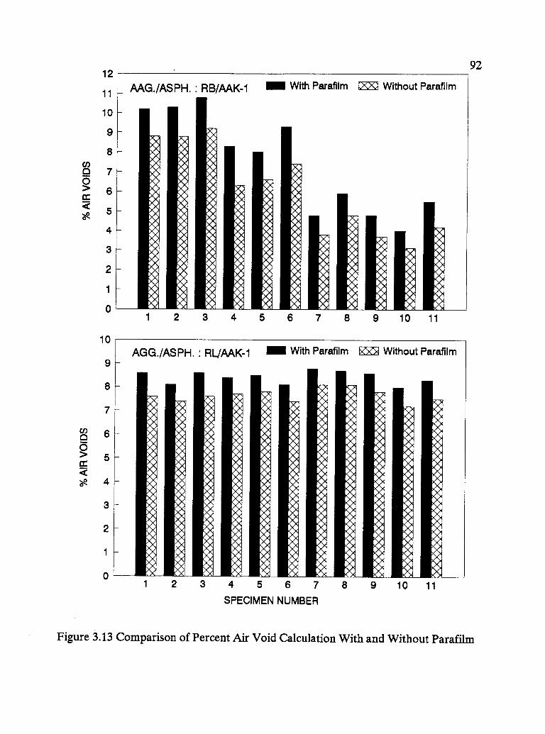
. - - : . .WA .
VIr r I
4 40
4 40 I 0
4
t00 0 44 IIs 4
0 I4
0 I 0 40 0 I rt. 40 I 4 I
4 4I4 4 4
0 0. 4 4
0 44. 0 0 4 I I
4 40 0
4 41 0
: 414 40 1 I4 4 4
0 I4 4 4
0 0 040 : 0 0
0 4 I 1 1 44 4 4
1 I I4 4
40 0 I0 0 4 I
4 40 I 1
4 4I 06-4 -4 -4 _4
lai
;
-.,
: :
to
:
. .
H
:. :,
.:
I oo . I I I ' o S I . I 1 5.11
.
, ':
:
:
:
A
4

93
included in the percent air voids in the case "with parafilm," and excluded in the case
"without parafilm."
The resulting air voids from the RB/AAK-1 mixture with parafilm are 1.5% higher
than without parafilm for the same mixture. Aggregate type has a significant effect
on the difference, because aggregate texture and aggregate shape influence specimen
surface air voids which are included in the percent air voids in the case "with
parafilm," and excluded in the case "without parafilm."
AASHTO T-283 is part of the water sensitivity testing program. As part of this
procedure specimen specific gravity is required for three conditions: dry condition,
partially saturated, and water conditioned. Wrapping partially saturated and water
conditioned specimens with parafilm is not practical because under these
circumstances the specimens continuously drain water. Due to this difficulty, it was
decided to test AASHTO T-283 dry specimens using both methods and test partially
saturated and water conditioned specimens by only the "without parafilm" method.
Degree of saturation and water conditioning criteria on AASHTO T-283 test will be
based on "without" parafilm specific gravities, saturated surface dry weight.
The ECS testing program was based only on specific gravity and air voids calculated
from ASTM D 1188 "with parafilm" wrapping, because this procedure has an
advantage over the ASTM D 2726 in that the parafilm keeps the specimen dry.
Another advantage over ASTM D 1188 is that the parafilm can be removed easily,
and the specimen is not contaminated.
94
3.3 Environmental Conditioning System (ECS)
The testing program using the ECS was previously discussed in section 2. The
experimental plan (Figure 2.1) shows a matrix of the variables being evaluated. Not
all of the nine conditioning codes, or "cells", for each permeability level were
completed on each asphalt-aggregate combination. Specimens 4-in. in diameter by
4-in. high were used for the ECS testing program. Only one combination, RL
aggregate, was tested for all the variables and the remaining three combinations were
tested for only the extreme conditions. Figure 3.14 shows the combinations tested
for each conditioning code (matrix cell). All the water conditioning codes shown in
Figure 2.1 were performed with repeated loading except the freezing and dry
conditioning codes. The testing of open graded mixtures has been accomplished after
modifying the test setup, which is discussed in Chapter 4.
Table 3.8 shows all the test results of the development phase of the ECS. During the
early stages of ECS (early 1990) testing, numerous 4-in. diameter by 2.5-in. high
specimens were tested for several conditioning codes and these results are included
in Appendix B. Because a 4 in. high specimen was established for the ECS testing
(as discussed earlier), only 4-in. high specimens results were used in the following
analysis sections.

HOT 60C
DRY MOIST
6
.4
12
1.0
D.8
D.8
0.46 le
6 12 18
HC
LD
D
HD
LE
E
HE
4
2
0
6
4
LF
HF
12 4
LG
1.4
12
1.0
0.8
0.6
0.4
-4.4
1.2
1.0
/.8
1.4
1.2
1.0-
G 0.8
0.6
0.4
HG HH
1.6
1.4
12
1.0
0.8
6
HI
Figure 3.14 Summary of Plots of Different Conditioning Levels
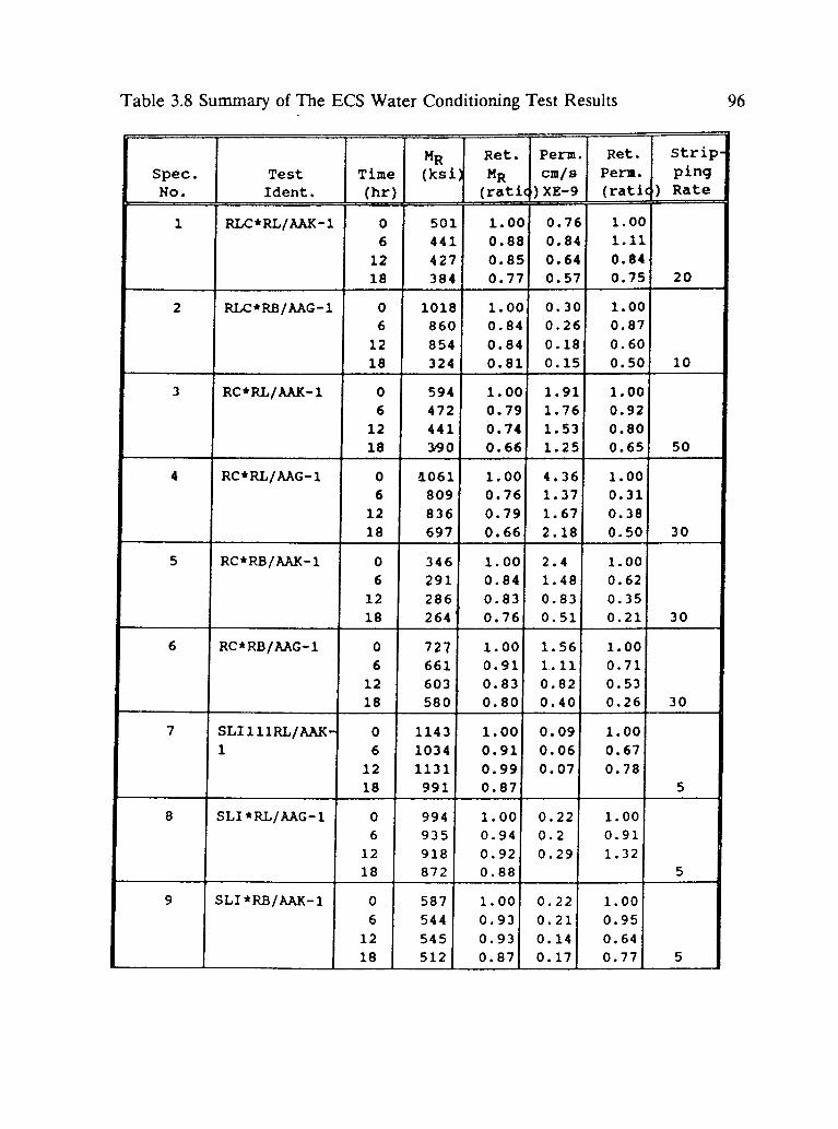
Table 3.8 Summary of The ECS Water Conditioning Test Results 96
Spec.No.
TestIdent.
Time(hr)
MR(ksi)
Ret.
MR(ratio)XE-9
Perm.
cm/s
Ret.
Perm.(ratio)
Strip-pingRate
1 RLC*RL/AAK-1 0 501 1.00 0.76 1.00
6 441 0.88 0.84 1.11
12 427 0.85 0.64 0.84
18 384 0.77 0.57 0.75 20
2 RLC*RB/AAG-1 0 1018 1.00 0.30 1.00
6 860 0.84 0.26 0.87
12 854 0.84 0.18 0.60
18 324 0.81 0.15 0.50 10
3 RC*RL/AAK-1 0 594 1.00 1.91 1.00
6 472 0.79 1.76 0.92
12 441 0.74 1.53 0.80
18 390 0.66 1.25 0.65 50
4 RC*RL/AAG-1 0 1061 1.00 4.36 1.00
6 809 0.76 1.37 0.31
12 836 0.79 1.67 0.38
18 697 0.66 2.18 0.50 30
5 RC*RB/AAK-1 0 346 1.00 2.4 1.00
6 291 0.84 1.48 0.62
12 286 0.83 0.83 0.35
18 264 0.76 0.51 0.21 30
6 RC*RB/AAG-1 0 727 1.00 1.56 1.00
6 661 0.91 1.11 0.71
12 603 0.83 0.82 0.53
18 580 0.80 0.40 0.26 30
7 SLI111RL/AAK- 0 1143 1.00 0.09 1.00
1 6 1034 0.91 0.06 0.67
12 1131 0.99 0.07 0.78
18 991 0.87 5
8 SLI*RL/AAG-1 0 994 1.00 0.22 1.00
6 935 0.94 0.2 0.91
12 918 0.92 0.29 1.3218 872 0.88 5
9 SLI*RB/AAX-1 0 587 1.00 0.22 1.00
6 544 0.93 0.21 0.95
12 545 0.93 0.14 0.64
18 512 0.87 0.17 0.77 5
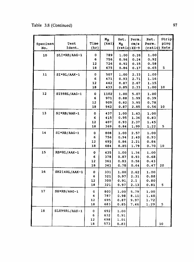
Table 3.8 (Continued) 97
SpecimenNo.
TestIdent.
Time(hr)
MR(ksi)
Ret.
MR(ratio)XE-9
Perm.cm/s
Ret.Perm.(ratio)
StrippingRate
10 SLI*RB/AAG-1 0 789 1.00 0.26 1.006 756 0.96 0.24 0.92
12 726 0.92 0.15 0.5818 675 0.86 0.17 0.65 5
11 SI*RL/AAK-1 0 507 1.00 2.33 1.006 471 0.93 2.71 1.16
12 442 0.87 2.67 1.1518 433 0.85 2.33 1.00 10
12 SI59RL/AAG-1 0 1102 1.00 5.07 1.006 971 0.88 1.99 0.39
12 909 0.82 3.95 0.7818 962 0.87 2.85 0.56 10
13 SI*RB/AAK-1 0 437 1.00 1.63 1.006 415 0.95 1.36 0.8312 407 0.93 2.37 1.4518 369 0.84 1.99 1.22 5
14 SI*RB/AAG-1 0 808 1.00 2.57 1.006 756 0.94 2.40 0.93
12 69p 0.86 2.21 0.8618 684 0.85 1.79 0.70 10
15 RB*RL/AAK-1 0 435 1.00 1.36 1.006 378 0.87 0.93 0.68
12 361 0.83 0.58 0.4318 341 0.78 0.64 0.47 20
16 SH214RL/AAK-1 0 331 1.00 2.62 1.006 321 0.97 2.31 0.88
12 300 0.91 2.1 0.8018 321 0.97 2.13 0.81 5
17 SH*RB/AAG-1 0 803 1.00 5.79 1.006 787 0.98 8.11 1.40
12 695 0.87 9.97 1.7218 683 0.85 7.46 1.29 5
18 SLH99RL/AAK-1 0 692 1.006 632 0.91
12 698 1.0118 573 0.83 10
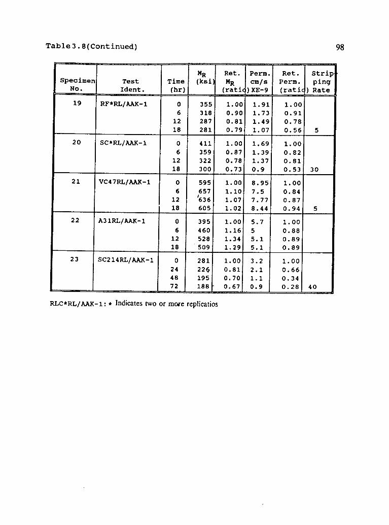
Table 3 . 8 (Continued) 98
SpecimenNo.
_
TestIdent.
Time(hr)
MR(ksi)
Ret.MR(ratio)XE-9
Perm.cm/s
Ret.Perm.(ratio)
StrippingRate
19 RF*RL/AAK-1 0 355 1.00 1.91 1.006 318 0.90 1.73 0.91
12 287 0.81 1.49 0.7818 281 0.79 1.07 0.56 5
20 SC*RL/AAK-1 0 411 1.00 1.69 1.006 359 0.87 1.39 0.82
12 322 0.78 1.37 0.8118 300 0.73 0.9 0.53 30
21 VC47RL/AAK-1 0 595 1.00 8.95 1.006 657 1.10 7.5 0.84
12)636 1.07 7.77 0.87
18 605 1.02 8.44 0.94 5
22 A31RL/AAK-1 0 395 1.00 5.7 1.006 460 1.16 5 0.88
12 528 1.34 5.1 0.8918 509 1.29 5.1 0.89
23 SC214RL/AAK-1 0 281 1.00 3.2 1.0024 226 0.81 2.1 0.6648 195 0.70 1.1 0.3472 188- 0.67 0.9 0.28 40
RLC*RL/AAK-1: * Indicates two or more replicatios

99
ECS-MR
Triaxial resilient modulus (ECS-MR) was performed using the ECS at 25 ° C on each
specimen in the dry condition and again following each water conditioning cycle.
Retained ECS-MR was calculated for each cycle as a ratio of ECS-MR after
conditioning to dry ECS-MR (before conditioning).
Conditioning duration (cycle-time) was investigated by conditioning two specimens
from the same material and same air void level for two cycle-durations (6 and 24 hrs)
and the test results are shown in Table 3.8 (specimens 20 and 23). Graphical display
and discussion are in Chapter 4.
Most of the previous research has been accomplished without incorporating the effect
of traffic on water damage. The effect of traffic was simulated in this study by
applying repeated loading on the specimen while conditioning it through temperature
cycles. ECS-MR and water permeability were monitored for two sets of specimens
that were water conditioned, one with static loading (10 in. Hg vacuum, equivalent
to 5 psi) and the other set with repeated loading (200 lb. or 17 psi). The data for
these two sets (Specimens 20 and 1) are shown in Table 3.8. The effect of repeated
loading is discussed later.
100
It is generally understood (without investigation) that the water is the best fluid to
be used for conditioning asphalt concrete specimens to investigate moisture-related
problems. But actually, in the field, there are pavements that show water damage
resulting from evaporation from the water table beneath the asphalt pavement. For
this reason, three fluids (air, vapor, and distilled water) were used to condition three
different specimens. Conditioning a specimen with vapor was conducted by adjusting
the environmental conditioning cabinet at temperature 60°C and at relative humidity
90%. Vapor was pulled through the specimen by vacuum (10 in. Hg). The vacuum
inlet inside the environmental cabinet was connected to a funnel to collect and direct
the air flow, and right after the funnel, a flow meter was connected to maintain the
vacuum level according to the ECS conditioning procedure (10 in. Hg). The same
vapor conditioning setup has been used to conduct "air" conditioning by maintaining
the same temperature (60°C) and adjusting relative humidity to 0%. For water
conditioning, the normal ECS setup was used to conduct hot-wet conditioning (C-
conditioning code) as described earlier for static loading.
Permeability and ECS-MR were monitored following conditioning cycles and the
results from the three specimens are shown in Table 3.8 (Specimens 21, 22, and 3).
The vapor conditioning setup was fabricated as shown in Figure 3.15.
In addition to the above investigations, the main ECS experiment included the effect
of the following variables:

FUNNEL
Flow Meter
Enviromental Conditioning Cabinet System
To Computer Loading System
A
CONTROL VALVE VACUUM PUMP
VACUUM REGULATOR
FLOW MANOMETER
WATER TRAP
Figure 3.15 Schematic Drawing of Vapor Conditioning Setup
102
Vacuum level,
Air void level, and
Saturation level.
Permeability
It is generally understood that the higher the air voids, the higher permeability and
the more water that can penetrate (and remain, to some degree) in an asphalt
pavement. But when aggregate type and aggregate gradation are variables, mixtures
may have similar air voids but the permeability of one may be as much as twice that
of the other one. Hein and Schmidt (1961) studied air permeability of asphalt
concrete and concluded that permeability, when influenced by gradation changes, is
not always proportional to void content. Most of the customary conceptions (i.e.,
permeability is proportional to voids content) are concluded from studies conducted
on similar aggregates.
Since the permeability represents both the volume of air voids and their structure,
this parameter may be a better indicator of performance than voids alone. In this
study, permeability was measured using air for each specimen before beginningwater
conditioning. Table 3.9 shows air permeability and air voids results. Since water
permeability, which is measured during water conditioning, is not the true
permeability because the specimen is not fully saturated, this measurement is used

103Table 3.9 Permeability Versus Percent Air Voids
Spec.no.
Asph.-Agg.Type
AirVoids
(%)
AirPerm.X E-9(cm/s)
Spec.no.
Asph.-Agg.Type
AirVoids
(%)
AirPerm.X E -9(cm/s)
Spec.no.
Asph.-Agg.Type
AirVoids
(%)
AirPerm.X E -9(cm/s)
1 RL/AAK 5.0 1.80 44 RL/AAK 5.1 2.94 87 RL/AAK 8.0 3.302 RL/AAK 4.5 1.30 45 RL/AAK 6.4 0.17 88 RL /AAK 7.2 2.603 RL/AAK 7.1 7.48 46 RL/AAK 4.9 13.85 89 RL/AAK 7.8 3.204 RL/AAK 7.0 3.40 47 RL/AAK 4.4 9.03 90 RL/AAK 8.0 5.505 RL/AAK 7.1 3.40 48 RL/AAK 4.7 1.33 91 RL/AAK 8.5 5.776 RL/AAK 3.9 0.14 49 RL/AAK 6.7 2.58 92 RL/AAK 8.1 5.197 RL/AAK 7.7 5.42 50 RL/AAK 6.9 1.75 93 RL/AAK 8.1 4.968 RL/AAK 7.9 2.24 51 RL/AAK 6.0 0.89 94 RL/AAK 8.0 3.209 RL/AAK 7.9 4.37 52 RL/AAK 5.6 1.47 95 RL/AAK 7.6 4.60
10 RL/AAK 9.1 5.26 53 RL/AAK 5.3 1.20 96 RL/AAK 4.9 0.1511 RL/AAK 8.5 3.79 54 RL/AAK 5.5 4.48 97 RL/AAK 7.8 3.0512 RL/AAK 3.8 0.64 55 RL/AAK 7.4 7.20 98 RL/AAK 7.1 6.6113 RL/AAK 8.0 4.71 56 RL/AAK 7.4 7.25 99 RL/AAK 4.8 0.5214 RL/AA.K 8.9 3.25 57 RL/AAK 7.6 6.86 100 RL/AAK 9.0 5.7015 RL/AAK 8.8 5.21 58 RL/AAK 9.0 4.77 101 RL/AAK 7.9 4.2616 RL/AAK 8.0 4.78 59 RL/AAK 7.8 5.11 102 RL/AAK 9.2 2.8417 RL/AAK 6.8 2.61 60 RL/AAK 8.8 3.73 103 RL/AAK 8.2 3.8018 RL/AAK 9.0 5.70 61 RL/AAK 8.1 5.70 104 RL/AAK 8.3 4.9019 RL/AAK 8.4 2.46 62 RL/AAK 7.5 3.40 105 RL/AAK 8.6 7.7020 RL/AAK 6.1 0.22 63 RL/AAK 7.5 4.80 106 RL/AAK 9.1 13.3021 RL/AAK 6.5 0.19 64 RL/AAK 8.5 6.00 107 RL/AAK 8.6 5.0022 RL/AAK 7.0 7.50 65 RL/AAK 7.7 4.40 108 RL/AAK 8.3 5.9023 RL/AAK 4.2 6.80 66 RL/AAK 7.4 4.50 109 RL/AAK 9.3 L7824 RL/AAK 8.5 6.20 67 RL/AAK 7.8 5.40 110 RL/AAK 8.3 5.8125 RL/AAK 8.1 12.83 68 RL/AAK 7.2 3.20 111 RL/AAK 8.0 5.0326 RL/AAK 6.4 4.25 69 RL/AAK 7.6 3.30 112 RL/AAK 9.5 6.4627 RL/AAK 7.0 3.59 70 RL/AAK 7.4 4.10 113 RL/AAK 9.1 6.1028 RL/AAK 6.4 13.85 71 RL/AAK 7.6 4.20 114 RL/AAK 8.6 5.0029 RL/AAK 6.4 9.53 72 RL/AAK 7.7 4.40 115 RL/AAK 8.6 5.5030 RL/AAK 5.9 1.27 73 RL/AAK 7.4 4.50 116 RL/AAK 6.6 1.2031 RL/AAK 7.1 2.46 74 RL/AAK 8.1 5.70 117 RL/AAK 6.9 1.5032 RL/AAK 7.0 0.87 75 RL/AAK 7.8 5.40 118 RL/AAK 5.9 1.1733 RL/AAK 8.0 7.40 76 RL/AAK 7.5 4.80 119 RL/AAK 6.4 1.1034 RL/AAK 6.2 3.00 77 RL/AAK 8.5 6.00 120 RL/AAK 7.2 7.7235 RL/AAK 6.1 4.56 78 RL/AAK 7.5 3.40 121 RL/AAK 5.2 0.8336 RL/AAK 5.9 1.74 79 RL/AAK 7.8 3.40 122 RL/AAK 5.2 0.6937 RL/AAK 6.6 1.86 80 RL/AAK 7.7 3.40 123 RL/AAK 8.3 8.9538 RL/AAK 7.4 14.50 81 RL/AAK 8.0 3.60 124 RL/AAK 7.1 7.4839 RL/AAK 6.7 4.21 82 RL/AAK 8.3 3.60 125 RL/AAK 7.7 5.4240 RL/AAK 5.8 1.75 83 RL/AAK 7.9 3.40 126 RL/AAK 8.0 20.3841 RL/AAK 5.7 1.89 84 RL/AAK 7.0 2.70 127 RL/AAG 7.2 29.0442 RL/AAK 5.7 5.71 85 RL/AAK 7.7 3.00 128 RL/AAG 6.9 1.8343 RL/AAK 6.4 0.92 86 RL/AAK 7.2 2.90 129 RL/AAG 4.9 L03
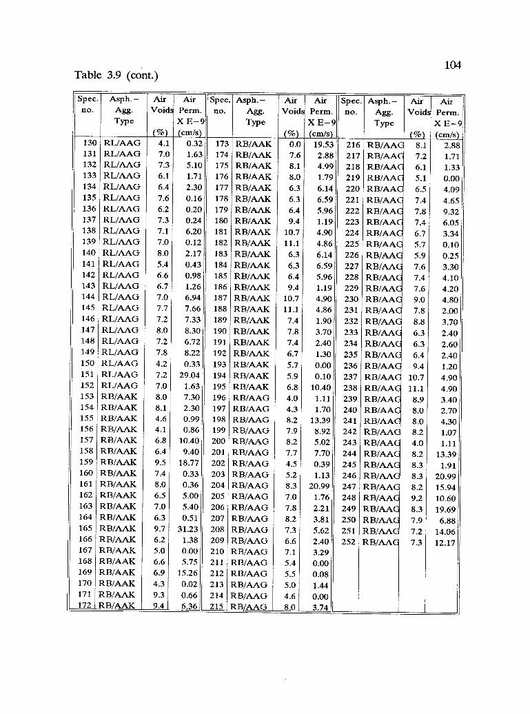
104Table 3.9 (cont.)
Spec.no.
Asph.-Agg.Type
AirVoids
(%)
AirPenn.X E-9(cm/s)
Spec.no.
Asph.-Agg.Type
AirVoids
(%)
AirPerm.X E-9(cm/s)
Spec.no.
Asph.-Agg.Type
AirVoids
(%)
AirPerm.X E-9(cm/s)
130 RL/AAG 4.1 0.32 173 RB/AAK 0.0 19.53 216 RB/AAG 8.1 2.88131 RL/AAG 7.0 1.63 174 RB/AAK 7.6 2.88 217 RB/AAG 7.2 1.71132 RL/AAG 7.3 5.10 175 RB/AAK 8.1 4.99 218 RB/AAG 6.1 1.33133 RL/AAG 6.1 1.71 176 RB/AAK 8.0 1.79 219 RB/AAG 5.1 0.00134 RL/AAG 6.4 2.30 177 RB/AAK 6.3 6.14 220 RB/AAG 6.5 4.09135 RL/AAG 7.6 0.16 178 RB/AAK 6.3 6.59 221 RB/AAG 7.4 4.65136 RL/AAG 6.2 0.20 179 RB/AAK 6.4 5.96 222 RB/AAG 7.8 9.32137 RL/AAG 7.3 0.24 180 RB/AAK 9.4 1.19 223 RB/AAG 7.4 6.05138 RL/AAG 7.1 6.20 181 RB/AAK 10.7 4.90 224 RB/AAG 6.7 3.34139 RL/AAG 7.0 0.12 182 RB/AAK 11.1 4.86 225 RB/AAG 5.7 0.10140 RL/AAG 8.0 2.17 183 RB/AAK 6.3 6.14 226 RB/AAG 5.9 0.25141 RL/AAG 5.4 0.43 184 RB/AAK 6.3 6.59 227 RB/AAG 7.6 3.30142 RL/AAG 6.6 0.98 185 RB/AAK 6.4 5.96 228 RB/AAG 7.4 4.10143 RL/AAG 6.7 1.26 186 RB/AAK 9.4 1.19 229 RB/AAG 7.6 4.20144 RL/AAG 7.0 6.94 187 RB/AAK 10.7 4.90 230 RB/AAG 9.0 4.80145 RL/AAG 7.7 7.66 188 RB/AAK 11.1 4.86 231 RB/AAG 7.8 2.00146 RL/AAG 7.2 7.33 189 RB/AAK 7.4 1.90 232 RB/AAG 8.8 3.70147 RL/AAG 8.0 8.30 190 RB/AAK 7.8 3.70 233 RB/AAG 6.3 2.40148 RL/AAG 7.2 6.72 191 RB/AAK 7.4 2.40 234 RB/AAG 6.3 2.60149 RL/AAG 7.8 8.22 192 RB/AAK 6.7 1.30 235 RB/AAG 6.4 2.40150 RL/AAG 4.2 0.33 193 RB/AAK 5.7 0.00 236 RB/AAG 9.4 1.20151 RL/AAG 7.2 29.04 194 RB/AAK 5.9 0.10 237 RB/AAG 10.7 4.90152 RL/AAG 7.0 1.63 195 RB/AAK 6.8 10.40 238 RB/AAG 11.1 4.90153 RB/AAK 8.0 7.30 196 RB/AAG 4.0 1.11 239 RB/AAG 8.9 3.40154 RB/AAK 8.1 2.30 197 RB/AAG 4.3 1.70 240 RB/AAG 8.0 2.70155 RB/AAK 4.6 0.99 198 RB/AAG 8.2 13.39 241 RB/AAG 8.0 4.30156 RB/AAK 4.1 0.86 199 RB/AAG 7.9 8.92 242 RB/AAG 8.2 1.07157 RB/AAK 6.8 10.40 200 RB/AAG 8.2 5.02 243 RB/AAG 4.0 1.11158 RB/AAK 6.4 9.40 201 RB/AAG 7.7 7.70 244 RB/AAG 8.2 13.39159 RB/AAK 9.5 18.77 202 RB/AAG 4.5 0.39 245 RB/AAG 8.3 1.91160 RB/AAK 7.4 0.33 203 RB/AAG 5.2 1.13 246 RB/AAG 8.3 20.99161 RB/AAK 8.0 0.36 204 RB/AAG 8.3 20.99 247 RB/AAG 8.2 15.94162 RB/AAK 6.5 5.00 205 RB/AAG 7.0 1.76 248 RB/AAG 9.2 10.60163 RB/AAK 7.0 5.40 206 RB/AAG 7.8 2.21 249 RB/AAG 8.3 19.69164 RB/AAK 6.3 0.51 207 RB/AAG 8.2 3.81 250 RB/AAG 7.9 6.88165 RB/AAK 9.7 31.23 208 RB/AAG 7.3 5.62 251 RB/AAG 7.2 14.06166 RB/AAK 6.2 1.38 209 RB/AAG 6.6 2.40 252 RB/AAG 7.3 12.17167 RB/AAK 5.0 0.00 210 RB/AAG 7.1 3.29168 RB/AAK 6.6 5.75 211 RB/AAG 5.4 0.00169 RB/AAK 6.9 15.26 212 RB/AAG 5.5 0.08170 RB/AAK 4.3 0.02 213 RB/AAG 5.0 1.44171 RB/AAK 9.3 0.66 214 RB/AAG 4.6 0.00172 RB/AAK 9.4 6.36 215 RB/AAG 8.0 3.74
105
only as a relative indicator for air voids structure change due to water conditioning
as well as repeated loading.
Visual Evaluation
Visual evaluation of asphalt concrete specimens is a method used to determine the
percentage of retained asphalt coating on the aggregate after the sample has been
water conditioned. The visual evaluation method is fundamental in boiling tests and
static immersion tests. The primary shortcoming with this method is the subjective
nature of the results. Sometimes, in an attempt to limit the subjectivity of the visual
evaluation, rating boards or patterns, similar to those shown in Figure 3.16 are used
to aid the rater and help establish consistency in the results. Another method is the
use of more than one rater and then averaging the results.
In addition, differences in how and when specimens are evaluated can further
decrease the precision of the results. For example, for boiling tests, it is common to
place the sample on a paper towel and evaluate the mixture when it has dried.
Parker and Wilson (1986) found that the timing of the evaluation can play a
significant role in percent coating rating given to an asphalt sample after the boiling
test. This is due to the hot asphalt recoating the stripped aggregate from the
remaining asphalt. Although the asphalt on the aggregate is thinner, the visual
evaluation does not account for the film thickness. This is in contrast to the static
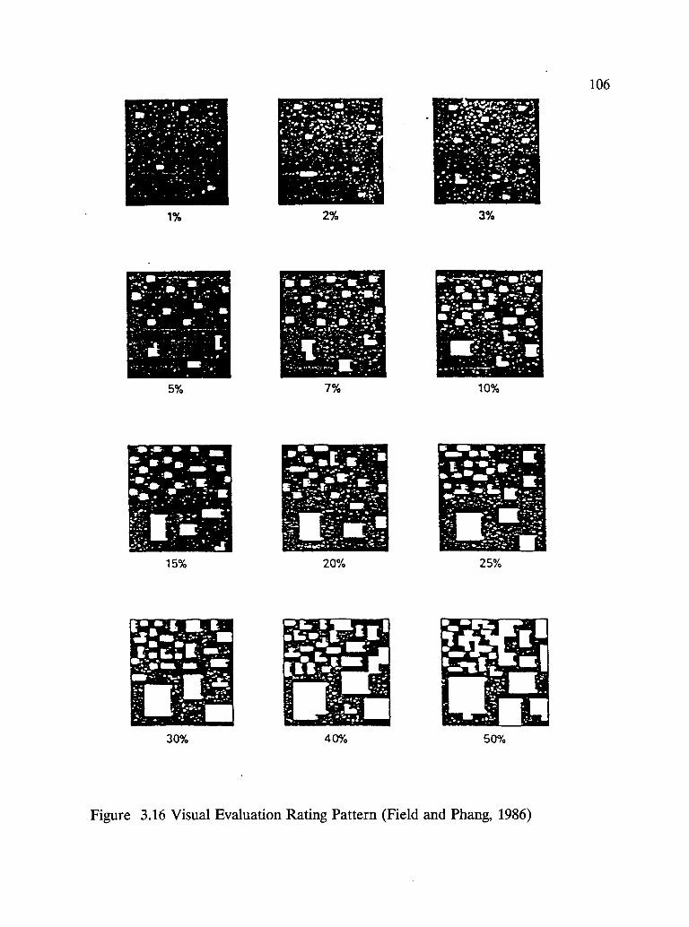
WO
.1 V.A
.I
I01:
Irearil1?..'
jU. 4
a

107
immersion tests where the sample is typically rated while still in the container and
immersed in water.
The method used in NCHRP 246 recommends that following the indirect tensile test,
the specimen be split open and the percent stripping be evaluated on the fractured
interior faces. Lottman (1982) used a stereo zoom microscope to estimate the
percent stripping in the fine aggregate and a magnifying glass for the coarse
aggregate, then calculated total percent stripping by pro-rating each fraction on a
60-40 basis. Based on others' experience, a visual evaluation technique was modified
for use in this study by considering the above problems of subjectivity. The new
visual evaluation technique reduced the rating patterns from the 12 levels, shown in
Figure 3.16, to only 6 levels (5, 10, 20, 30, 40, and 50%) and is described in
Chapter 4. This modification makes it practical and easy to distinguish between the
detail levels.
108
4. DISCUSSION AND ANALYSIS OF TEST RESULTS
In Chapter 2, it was pointed out that the ECS testing program was designed to
answer the most important questions related to the performance of mixtures in the
presence of water. From the test results (Table 3.8), and according to the
experiment design (Figure 2.1), the effect of the following variables on mixtures
response to water conditioning were analyzed in some detail:
Mixture Variables
1 - Aggregate type
2 - Asphalt type
3 - Air voids level
Conditioning Variables
1 Conditioning fluid
2 - Conditioning temperature
3 Vacuum level
4 - Repeated loading
109
5 - Conditioning time
4.1 Effect of Mixture Variables
Mixture variables are more limited than the conditioning variables, both in terms of
the number of the variables and in terms of simulating the real pavement, as shown
in Table 2.1. At this point in the study, only the three mixture variables will be
discussed in this section.
Aggregate Type
The two aggregates used are RB and RL from MRL materials. RL is known as a
stripping aggregate and RB is known as a non-stripper. The overall retained strength
was monitored by performing resilient modulus (ECS-MR) following water
conditioning cycles. Retained modulus ratio was calculated by dividing the ECS-MR
after conditioning by the ECS-MR before conditioning. Figure 4.1 shows the retained
MR ratio for the two aggregates RL and RB with AAG-1 and AAK-1 asphalts. The
four mixtures were subjected to three hot-wet conditioning cycles (6-hour cycle) with
continuous repeated loading.
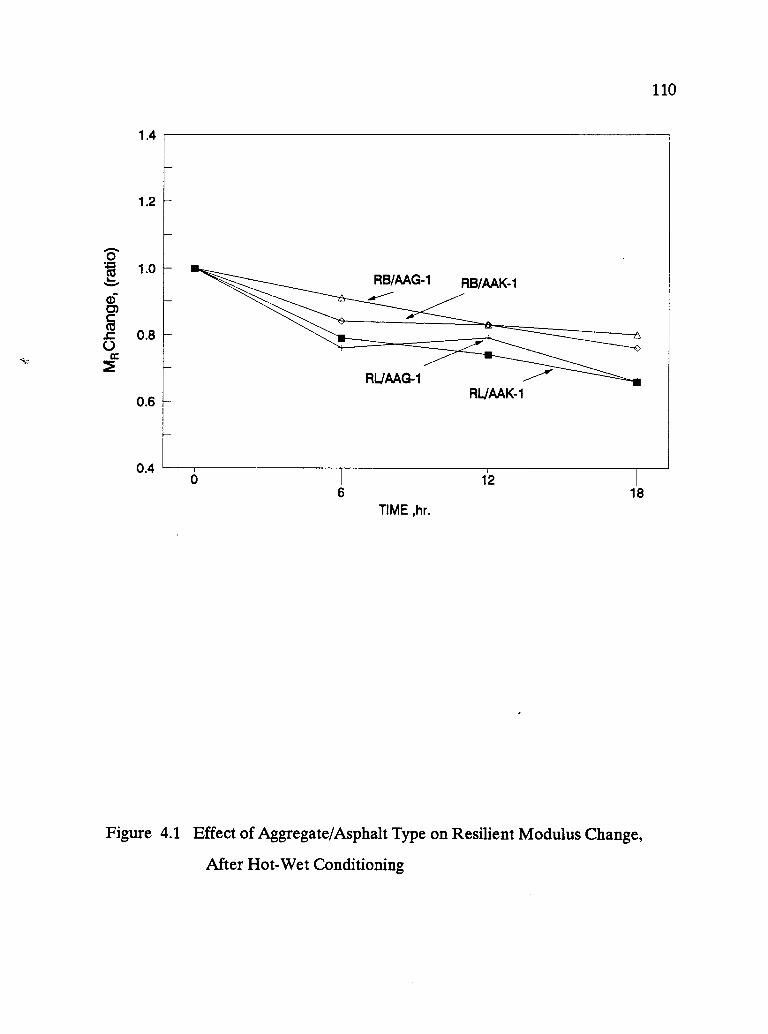
1.4
1.2
1.0
0.8
0.6
0.4
110
12 1
6 18TIME ,hr.
Figure 4.1 Effect of Aggregate/Asphalt Type on Resilient Modulus Change,
After Hot-Wet Conditioning
111
RB aggregate showed more resistance to water damage than RL, with both asphalts.
Another four sets of specimens from the four asphalt-aggregate combinations were
tested for freeze-wet conditioning. The results are shown in Figure 4.2. The results
showed that the effect of freezing cycles on MR is not significant (at this vacuum
level), and therefore no significant differences among the four tested materials.
In order to evaluate the differences presented graphically in Figure 4.1, the results
were statistically analyzed by using the General Linear Model Procedure (GLM) .
The GLM was selected in favor of the Analysis of Variance (ANOVA), because
GLM counts for unequal cell sizes, which are present in this study. The plan of this
phase of the project (development phase) was to evaluate the most related variables
in order to narrow them down and select those having the most effect on water
damage. This concept resulted in performing different test replicates according to
the effect of each conditioning code, as shown in Figure 2.1. Table 4.1 presents the
results of the GLM analysis for MR ratios at the end of the first, second, and third
cycles (times 6, 12, and 18 respectively). The difference between the MR ratios of the
three conditioning cycles is significant at the 90.0 % confidence level, except the
second cycle where the difference is significant at 80 percent.
The GLM (as shown here in a brief format) does not give enough information about
within treatments. So, a Least Significant Difference (LSD) was used to rank the
four combinations according to the aggregate and asphalt types.
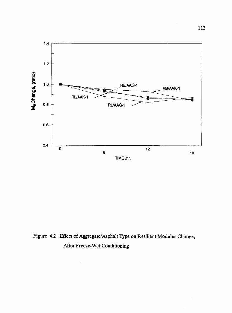
1.4
1.2
1.0
0.8
0.6
0.4
112
a1 126 18
TIME ,hr.
Figure 4.2 Effect of Aggregate/Asphalt Type on Resilient Modulus Change,
After Freeze-Wet Conditioning

113
Table 4.1 Analysis of Variance of the Difference Between MR Ratios AfterThree Hot-Wet Conditioning Cycles for the Four Asphalt-AggregateCombinations
TIME 6Sum of Mean (P = 0.10)
Source DF Squares Square F Value F Crit
Model 3 0.032 0.011 4.56* 3.07
Error 7 0.016 0.002
CorrectedTotal 10 0.049
TIME =12
Sum of Mean (P = 0.10)Source DF Squares Square F Value F Crit
Model 3 0.016 0.005 0.66 3.07
Error 7 0.057 0.008
CorrectedTotal 10 0.073
TIME =18
Sum of Mean (P = 0.10)Source DF Squares Square F Value F Crit
Model 3 0.045 0.015 3.27* 3.07
Error 7 0.032 0.004
CorrectedTotal 10 0.077
* : Significant at the 90.0 percent confidence level

114
Table 4.2 shows LSD ranking results of the three cycles, where the four combinations
were ranked logically according to their aggregate types. RB aggregate showed the
lowest water damage with a least significant difference less than 0.143 at the 95.0
percent confidence level for the first and third cycles. MR ratios after the second
cycle followed the same ranking, but with a lower Least Significant Difference (LSD)
between the means, which was 0.113 at the 80 percent confidence level. RL
aggregate experienced the highest water damage with the same statistical confidence
levels that showed RB aggregate with a low resistance to water damage. On the
other hand, asphalt type did not show a significant effect, which is discussed in the
following section.
This means that aggregate type has a significant response to the water conditioning
procedure, which confirms the graphical display and agrees with the known durability
of the two aggregates.
Asphalt Type
Two SHRP-MRL asphalts have been used for this study: Boscan AC-30 (AAK-1)
which has low temperature susceptibility, and California Valley AR-4000 (AAG-1)
which has high temperature-susceptibility. Figure 4.1 includes the effect of the two
asphalts with RL and RB aggregates.
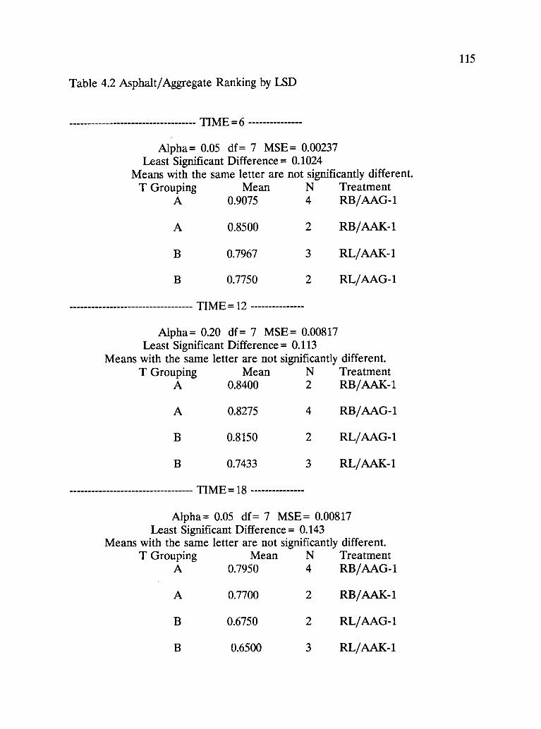
115
Table 4.2 Asphalt/Aggregate Ranking by LSD
TIME
Alpha= 0.05 df= 7 MSE= 0.00237Least Significant Difference = 0.1024
Means with the same letter are not significantly different.T Grouping Mean N Treatment
A 0.9075 4 RB/AAG-1
A 0.8500 2 RB/AAK-1
B 0.7967 3 RL/AAK-1
B 0.7750 2 RL/AAG-1
TIME =12
Alpha= 0.20 df= 7 MSE= 0.00817Least Significant Difference = 0.113
Means with the same letter are not significantly different.T Grouping Mean N Treatment
A 0.8400 2 RB/AAK-1
A 0.8275 4 RB/AAG-1
B 0.8150 2 RL/AAG-1
B 0.7433 3 RL/AAK-1
TIME =18
Alpha= 0.05 df= 7 MSE= 0.00817Least Significant Difference = 0.143
Means with the same letter are not significantly different.T Grouping Mean N Treatment
A 0.7950 4 RB/AAG-1
A 0.7700 2 RB/AAK-1
B 0.6750 2 RL/AAG-1
B 0.6500 3 RL/AAK-1
116
The difference between the two plots of AAK-1 asphalt with RL and RB aggregates
is not significant. Similarly, the difference between the two plots of AAG-1 asphalt
with RL and RB aggregates is not significant.
The same data for hot-wet conditioning which was used for Figure 4.1 were expressed
statistically in Tables 4.2 after conducting the LSD, as pointed out above. And the
same table was used to show the ranking of the effect of asphalt types. As shown in
Table 4.2, asphalt type did not show a consistent response, since neither asphalt type
showed the same LSD ranking with the three cycles. For more clarification, a direct
comparison between the two asphalts with the same aggregate type (RB/AAG-1
versus RB/AAK-1) was conducted by using the GLM. The effect of asphalt type was
found not significant at a very low confidence level, less than 50 percent for the
second and third cycles and less than 80 percent for the first cycle, as shown in
Table 4.3. This means that the four combinations cannot be ranked according to
their asphalt types even within a small difference between their means and as low a
confidence level as 50 percent.
As shown earlier, specimens from the four asphalt-aggregate combinations were
subjected to three freeze-wet conditioning cycles. Figure 4.2 shows the retained
strengths for the two aggregates and two asphalts. The freeze-wet conditioning
showed no significant effect at this vacuum level (20 in. Hg) and for this number
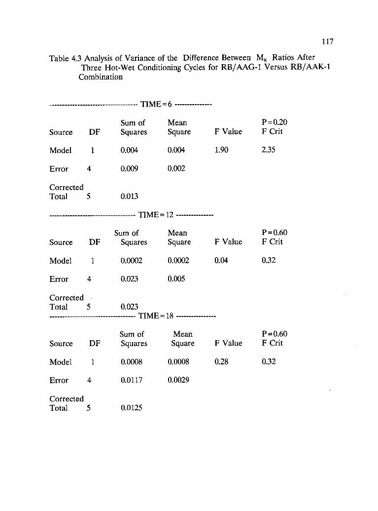
117
Table 4.3 Analysis of Variance of the Difference Between MR Ratios AfterThree Hot-Wet Conditioning Cycles for RB/AAG-1 Versus RB/AAK-1
Combination
TIME 6
Sum of Mean P = 0.20Source DF Squares Square F Value F Crit
Model 1 0.004 0.004 1.90 2.35
Error 4 0.009 0.002
CorrectedTotal 5 0.013
TIME =12
Sum of Mean P = 0.60Source DF Squares Square F Value F Crit
Model 1 0.0002 0.0002 0.04 0.32
Error 4 0.023 0.005
CorrectedTotal 5 0.023
TIME =18
Sum of Mean P = 0.60Source DF Squares Square F Value F Crit
Model 1 0.0008 0.0008 0.28 0.32
Error 4 0.0117 0.0029
CorrectedTotal 5 0.0125

118
of cycles (three 6-hour cycles). The same conclusion was drawn from GLM analysis,
which was conducted on the same data shown in Figure 4.2: that the difference
between the means is not significant at the 80 percent confidence level for the first
cycle, and at lower than 40 percent for the second and third cycles, as shown in Table
4.4. A trial of ranking the four combinations after freeze-wet conditioning cycles
was made by conducting the LSD, shown in Table 4.5. Although there is a ranking
at the 70.0 confidence level, it was not consistent throughout the three cycles with
either asphalt or aggregate type. This means there is no ranking for asphalt types nor
aggregate types at the typical confidence levels, such as 70 percent or more. So, it
was concluded that the hot-wet cycling is more severe than freeze-wet cycling.
Air Voids Level
As shown in the experiment plan, Figure 2.1, three permeability levels were
defined by three air voids levels; low such as 4 percent, medium such as 8 percent,
and high as more than 14 percent. Specimens with high air voids deformed under
the effect of high temperature and repeated loading, so a special conditioning
treatment was performed which is discussed later. Therefore, only two air voids
level are included in this discussion.
According to the experiment plan, two sets of specimens from the same asphalt-
aggregate combination with two air voids levels were subjected to three hot wet
conditioning cycles combined with a continuous repeated loading. Figure 4.3
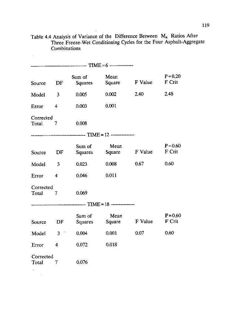
119
Table 4.4 Analysis of Variance of the Difference Between MR Ratios AfterThree Freeze-Wet Conditioning Cycles for the Four Asphalt-AggregateCombinations
TIME 6
Sum of Mean P = 0.20
Source DF Squares Square F Value F Crit
Model 3 0.005 0.002 2.40 2.48
Error 4 0.003 0.001
CorrectedTotal 7 0.008
TIME 12
Sum of Mean P = 0.60
Source DF Squares Square F Value F Crit
Model 3 0.023 0.008 0.67 0.60
Error 4 0.046 0.011
CorrectedTotal 7 0.069
TIME 18
Sum of Mean P = 0.60
Source DF Squares Square F Value F Crit
Model 3 0.004 0.001 0.07 0.60
Error 4 0.072 0.018
CorrectedTotal 7 0.076
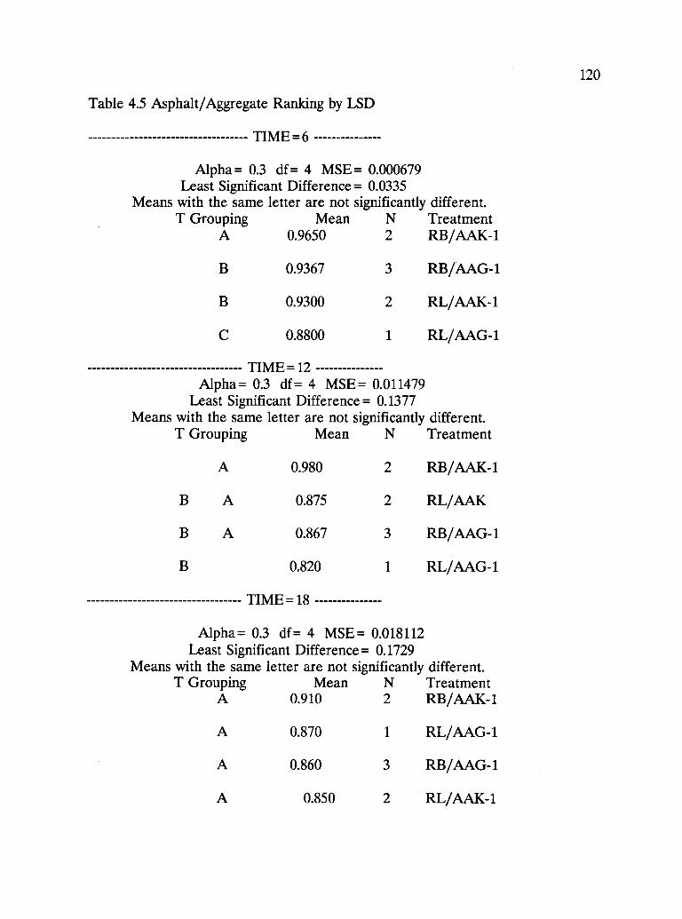
Table 4.5 Asphalt/Aggregate Ranking by LSD
TIME
Alpha= 0.3 df= 4 MSE= 0.000679Least Significant Difference = 0.0335
Means with the same letter are not significantly different.T Grouping Mean N
A 0.9650 2
B 0.9367 3
B 0.9300 2
C 0.8800 1
TIME =12
TreatmentRB/AAK-1
RB/AAG-1
RL/AAK-1
RL/AAG-1
Alpha= 0.3 df= 4 MSE= 0.011479Least Significant Difference = 0.1377
Means with the same letter are not significantly different.T Grouping Mean N
A 0.980
B A 0.875
B A 0.867
B 0.820
TIME-18
Treatment
2 RB/AAK-1
2 RL/AAK
3 RB/AAG-1
1 RL/AAG-1
Alpha= 0.3 df= 4 MSE= 0.018112Least Significant Difference = 0.1729
Means with the same letter are not significantly different.T Grouping Mean N Treatment
A 0.910
A 0.870
A 0.860
A 0.850
2 RB/AAK-1
1 RL/AAG-1
3 RB/AAG-1
2 RL/AAK-1
120
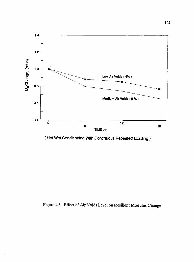
1.4
1.2
1.0
0.8
0.6
0.4
121
Low Air Voids ( 4% )
Medium Air Voids ( 8 % )
O6
TIME ,hr.
12 I
18
( Hot Wet Conditioning With Continuous Repeated Loading )
Figure 4.3 Effect of Air Voids Level on Resilient Modulus Change
122
shows the average of retained modulus ratios for each set. Specimen with high air
voids (8 percent) showed more significant water damage than specimens with low air
voids (4 percent).
A GLM statistical analysis was performed on the data and the results in Table 4.6
show that the effect of air voids is significant at the 90 percent confidence level.
Also, the LSD was conducted to show the ranking of MR ratios according to their
air voids and the results are in Table 4.7. MR ratios of the three cycles were ranked
significantly based on their air voids levels at the 90 confidence level with a least
significant difference more than 0.071. Specimens with low air voids showed more
resistance to water damage, because of their low accessibility to water penetration.
The result of these comparisons confirms the very important role of air voids on the
asphalt concrete response to water conditioning, and additional details are discussed
later.
4.2 Effect of Conditioning Variables
It has been observed that there is a significant variation among the current
methods in the final evaluation of a resistance of an asphalt concrete mixture to
water damage (Terrel and Shute 1989). Since most of the structural evaluation
techniques are usually the same, using either the resilient modulus or the tensile
strength, the source of the variations is mainly the conditioning techniques.

123
Table 4.6 Analysis of Variance of the Difference Between MR Ratios ofSpecimen With Two Air Voids Levels
TIME-6
Sum of Mean P=0.10Source DF Squares Square F Value F Crit
Model 1 0.008 0.008 5.60* 5.53
Error 3 0.004 0.001
CorrectedTotal 4 0.013
TIME =12Sum of Mean P =0.10
Source DF Squares Square F Value F Crit
Model 1 0.015 0.015 13.53* 5.50
Error 3 0.003 0.001
CorrectedTotal 4 0.018
TIME =18Sum of Mean P=0.10
Source DF Squares Square F Value F Crit
Model 1 0.016 0.016 6.39* 5.50
Error 3 0.007 0.002
CorrectedTotal 4 0.023
* : Significant at the 90.0 percent confidence level

124
Table 4.7 Asphalt/Aggregate Ranking by LSD Based on Air Voids Level
TIME-6
Alpha = 0.1 df= 3 MSE= 0.001489Least Significant Difference= 0.0829
Means with the same letter are not significantly different.
T Grouping Mean N Void Level
A 0.8800 2 Low
B 0.7967 3 High
TIME =12
Alpha = 0.1 df= 3 MSE = 0.001106Least Significant Difference = 0.0714
Means with the same letter are not significantly different.
T Grouping Mean N Void Level
A 0.8550 2 Low
B 0.7433 3 High
TIME =18
Alpha = 0.1 df = 3 MSE = 0.002483Least Significant Difference= 0.1071
Means with the same letter are not significantly different.
T Grouping Mean N Void Level
A 0.7650 2 Low
B 0.6500 3 High
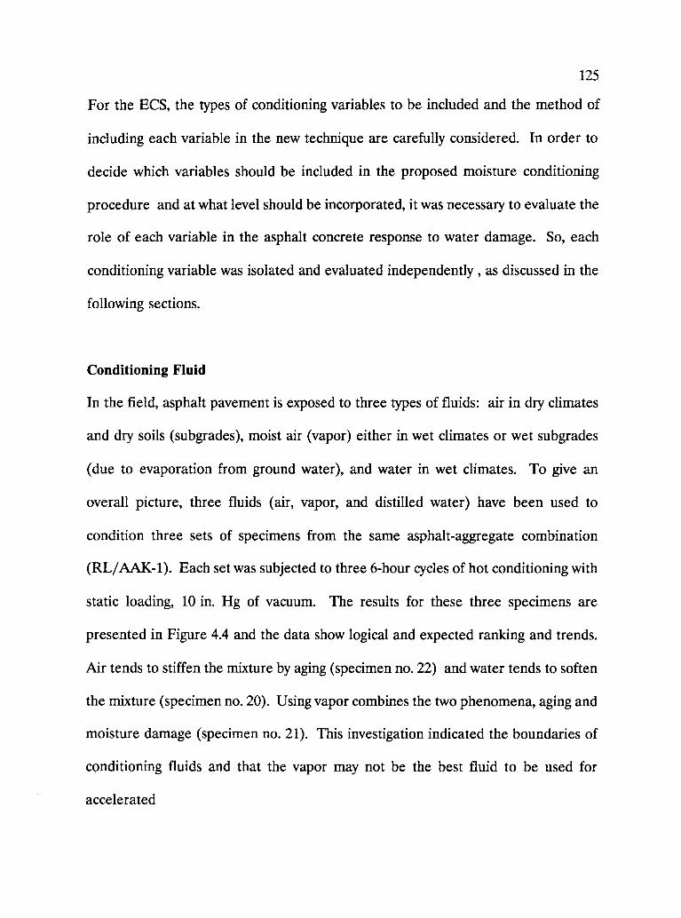
125
For the ECS, the types of conditioning variables to be included and the method of
including each variable in the new technique are carefully considered. In order to
decide which variables should be included in the proposed moisture conditioning
procedure and at what level should be incorporated, it was necessary to evaluate the
role of each variable in the asphalt concrete response to water damage. So, each
conditioning variable was isolated and evaluated independently , as discussed in the
following sections.
Conditioning Fluid
In the field, asphalt pavement is exposed to three types of fluids: air in dry climates
and dry soils (subgrades), moist air (vapor) either in wet climates or wet subgrades
(due to evaporation from ground water), and water in wet climates. To give an
overall picture, three fluids (air, vapor, and distilled water) have been used to
condition three sets of specimens from the same asphalt-aggregate combination
(RL/AAK-1). Each set was subjected to three 6-hour cycles of hot conditioning with
static loading, 10 in. Hg of vacuum. The results for these three specimens are
presented in Figure 4.4 and the data show logical and expected ranking and trends.
Air tends to stiffen the mixture by aging (specimen no. 22) and water tends to soften
the mixture (specimen no. 20). Using vapor combines the two phenomena, aging and
moisture damage (specimen no. 21). This investigation indicated the boundaries of
conditioning fluids and that the vapor may not be the best fluid to be used for
accelerated
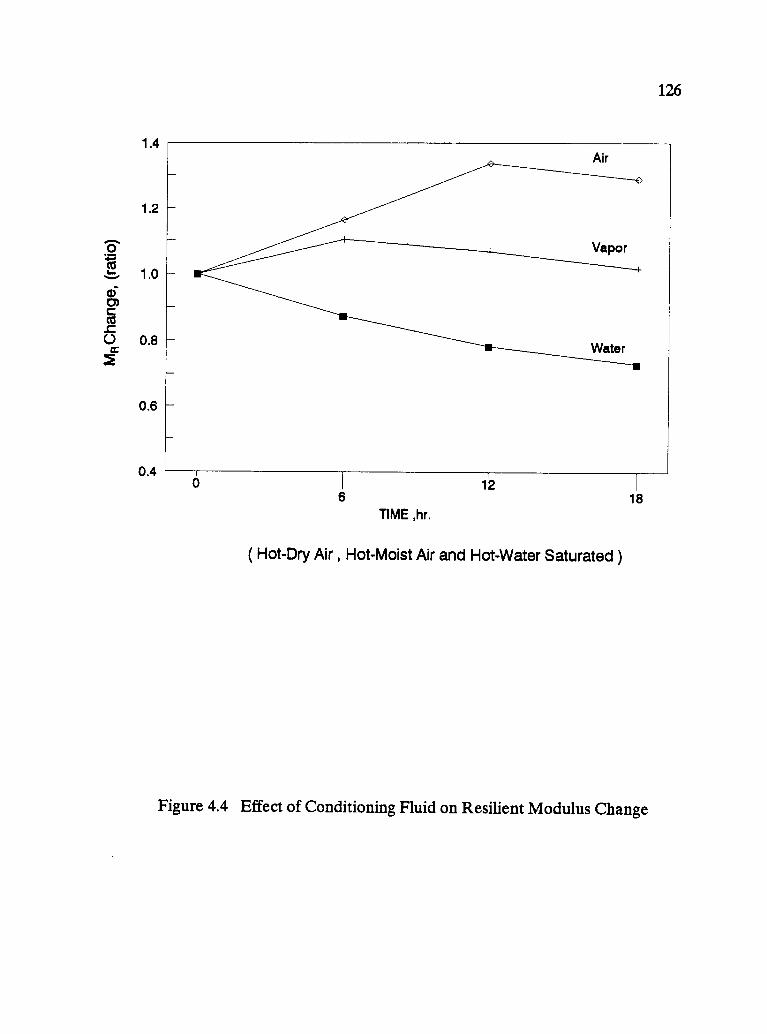
1.4
1.2
1.0
0.8
0.6
0.4
126
---
Air
Vapor
Water
a
O1 12
1
6TIME ,hr.
( Hot-Dry Air , Hot-Moist Air and Hot-Water Saturated )
18
Figure 4.4 Effect of Conditioning Fluid on Resilient Modulus Change
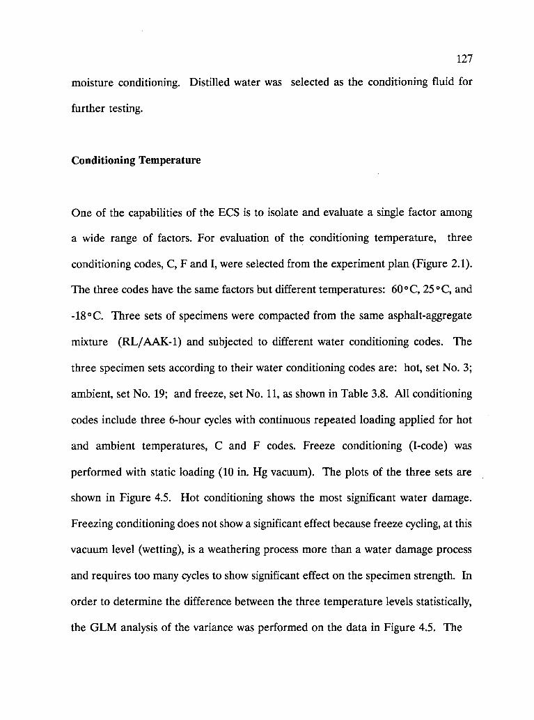
127
moisture conditioning. Distilled water was selected as the conditioning fluid for
further testing.
Conditioning Temperature
One of the capabilities of the ECS is to isolate and evaluate a single factor among
a wide range of factors. For evaluation of the conditioning temperature, three
conditioning codes, C, F and I, were selected from the experiment plan (Figure 2.1).
The three codes have the same factors but different temperatures: 60 °C, 25 °C, and
-18 °C. Three sets of specimens were compacted from the same asphalt-aggregate
mixture (RL/AAK-1) and subjected to different water conditioning codes. The
three specimen sets according to their water conditioning codes are: hot, set No. 3;
ambient, set No. 19; and freeze, set No. 11, as shown in Table 3.8. All conditioning
codes include three 6-hour cycles with continuous repeated loading applied for hot
and ambient temperatures, C and F codes. Freeze conditioning (I-code) was
performed with static loading (10 in. Hg vacuum). The plots of the three sets are
shown in Figure 4.5. Hot conditioning shows the most significant water damage.
Freezing conditioning does not show a significant effect because freeze cycling, at this
vacuum level (wetting), is a weathering process more than a water damage process
and requires too many cycles to show significant effect on the specimen strength. In
order to determine the difference between the three temperature levels statistically,
the GLM analysis of the variance was performed on the data in Figure 4.5. The
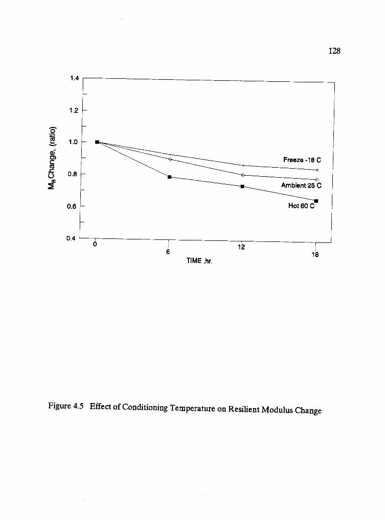
1.4
1.2
1.0
0.8
0.6
0.4
128
_Freeze -18 C
s
Ambient 25 C
Hot 60 C
af
612
TIME ,hr.18
Figure 4.5 Effect of Conditioning Temperature on Resilient Modulus Change

129
results of the statistical analysis for the three cycles are summarized in Table 4.8.
Significant differences were found among the three temperature levels at the 90
percent confidence level. The LSD was carried out to rank the impacts of the
temperature on MR ratio. Table 4.9 shows that there is a significant ranking at the
90 percent confidence level, where the specimen subjected to 60°C showed the
highest water damage, while the specimen subjected to -18°C showed the lowest
water damage. This means that the highest temperature is the highest water damage,
because high temperature accelerates water penetration into the specimen. Finally,
it was concluded that the hot, 60°C, cycling is appropriate to simulate and accelerate
field conditions in the hot climates. Hot and freeze, 60°C and -18°C respectively,
cycling is better to simulate the mechanism of the deterioration process in the cold
climates.
Vacuum Level
Another concern about water conditioning was the effect of degree of saturation. In
the ECS water conditioning procedure, the degree of saturation is defined by a
standardized vacuum level. The wetting vacuum level, prior to the water
conditioning cycling, is either 10-in. Hg for "moist" level or 20-in. Hg for "saturated"
level. A vacuum level of 10-in. Hg is then maintained during
conditioning cycles. Vacuum level appears to be more representative for the ECS
procedure because retaining some vacuum (10-in.) during water conditioning cycles

130
Table 4.8 Analysis of Variance of the Difference Between MR Ratios AfterThree Conditioning Cycles With Three Temperature Levels
TIME 6
Sum of Mean P = 0.10Source DF Squares Square F Value F Crit
Model 2 0.024 0.012 36.80* 4.32
Error 4 0.001 0.0003
CorrectedTotal 6 0.026
TIME 12Sum of Mean P = 0.10
Source DF Squares Square F Value F Crit
Model 2 0.021 0.010 4.47* 4.32
Error 4 0.009 0.002
CorrectedTotal 6 0.030
TIME 18
Sum of Mean P=0.10Source DF Squares Square F Value F Crit
Model 2 0.055 0.027 9.82* 4.32
Error 4 0.011 0.003
CorrectedTotal 6 0.066
* : Significant at the 90.0 percent confidence level
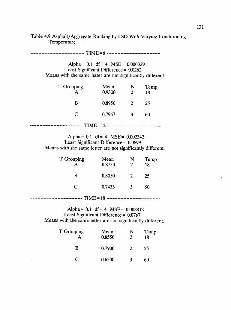
131
Table 4.9 Asphalt/Aggregate Ranking by LSD With Varying ConditioningTemperature
TIME-6
Alpha= 0.1 df= 4 MSE= 0.000329Least Significant Difference = 0.0262
Means with the same letter are not significantly different.
T Grouping Mean N TempA 0.9300 2 18
B 0.8950 2 25
C 0.7967 3 60
TIME =12
Alpha= 0.1 df= 4 MSE= 0.002342Least Significant Difference = 0.0699
Means with the same letter are not significantly different.
T Grouping Mean N TempA 0.8750 2 18
B 0.8050 2 25
C 0.7433 3 60
TIME =18
Alpha= 0.1 df= 4 MSE= 0.002812Least Significant Difference = 0.0767
Means with the same letter are not significantly different.
T Grouping Mean N TempA 0.8550 2 18
B 0.7900 2 25
C 0.6500 3 60

132
maintains a constant degree of wetting better than for static immersion conditioning.
In order to investigate the effect of vacuum level, similar specimens (RL/AAK-1)
were subjected to four different conditioning codes: B, C, H, and I (Figure 2.1). The
four codes were divided into two sets. The two sets according to their conditioning
codes are as follows:
Freeze conditioning H and I: Set No. 16 and No. 11
Hot - conditioning B and C: Set No. 15 and No. 3, respectively
(Table 3.8)
Figure 4.6 shows retained MR for the freeze-conditioned specimens. There is no
significant difference between the two levels because generally freezing cycles do not
affect asphalt mixture strength (without also cycling hot) which was explained earlier.
Figure 4.7 shows retained MR for hot conditioning. High vacuum had more
significant effect than low vacuum level because at high temperatures, water
penetration increases, resulting in more water damage. By comparing the stripping
rates as shown in Table 3.8, sets No. 16 and No. 11 (freeze) experienced similar
stripping rates of 5 and 10 percent, respectively. By contrast, there is a significant
difference between the stripping rates resulted from the two vacuum levels with hot
conditioning; set No. 15 experienced 20 percent while set No. 3 experienced 50
percent stripping rate. The above comparison indicates that 20-in. vacuum level is
an oppropriate technique to be used to accelerate the saturation process.
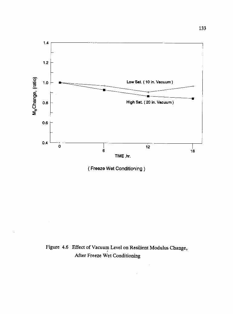
1.4
1.2
1.0
0.8
0.6
0.4
133
_ Low Sat. ( 10 in. Vacuum )
_ High Sat. ( 20 in. Vacuum )
a6
TIME ,hr.
( Freeze Wet Conditioning )
121
18
Figure 4.6 Effect of Vacuum Level on Resilient Modulus Change,
After Freeze Wet Conditioning
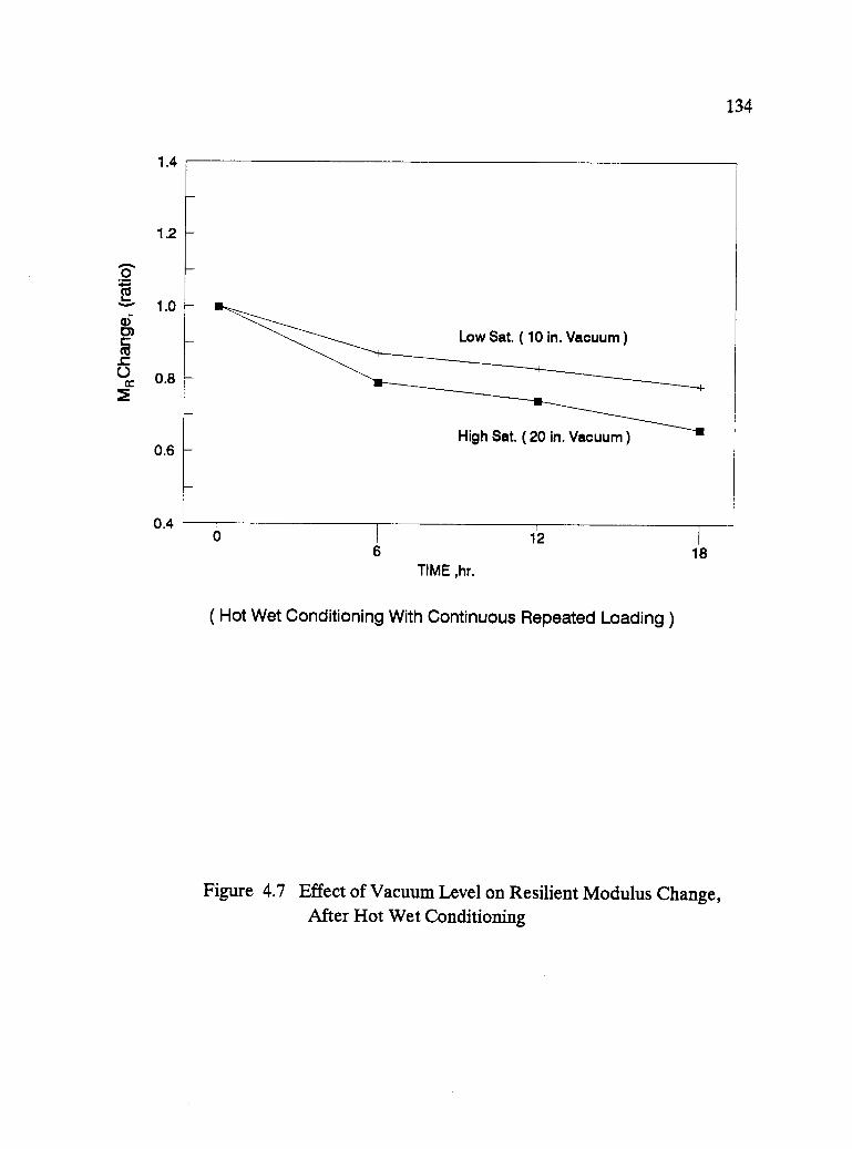
1.4
1.2
1.0
0.8
0.6
0.4
134
Low Sat. ( 10 in. Vacuum )
High Sat. ( 20 in. Vacuum )
a6
TIME ,hr.
12
( Hot Wet Conditioning With Continuous Repeated Loading )
1
18
Figure 4.7 Effect of Vacuum Level on Resilient Modulus Change,After Hot Wet Conditioning
135
In order to confirm the above findings, the data were re-analyzed statistically. Since
the effect of vacuum level with freezing cycles is obviously not significant (Figure
4.6), only the data of hot conditioning (B and C) were statistically analyzed. The
GLM was carried out on the data shown in Figure 4.7. The statistical analysis
results, Table 4.10, showed a significant difference between the two vacuum levels
at the 90 percent confidence level. In addition to the GLM analysis, the MR ratios
of hot conditioning cycles (Figure 4.7) were ranked statistically according to their
vacuum levels by conducting the LSD. As shown in Table 4.11, the two levels were
ranked statistically significant at the 90 percent confidence level with a least
significant difference less than 0.044.
From the above results, it was concluded that the 20 in. Hg vacuum level for
"wetting" stage and the 10 in. Hg retained vacuum during water conditioning cycles
(either hot or freeze cycles) are appropriate for the "standard" ECS water
conditioning procedure.
Repeated Loading
The general approach to this study has been to test the asphalt concrete under
conditions as similar as possible to those likely to occur in the field. One of the
most difficult variables to simulate in asphalt concrete testing is the traffic loading.
A previous study found that heavy traffic volume appeared to increase the rate of
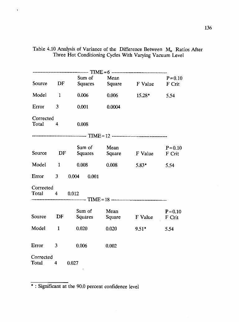
136
Table 4.10 Analysis of Variance of the Difference Between MR Ratios AfterThree Hot Conditioning Cycles With Varying Vacuum Level
TIME 6Sum of Mean P = 0.10
Source DF Squares Square F Value F Crit
Model 1 0.006 0.006 15.28* 534
Error 3 0.001 0.0004
CorrectedTotal 4 0.008
TIME =12
Sum of Mean P = 0.10Source DF Squares Square F Value F Crit
Model 1 0.008 0.008 5.83* 5.54
Error 3 0.004 0.001
CorrectedTotal 4 0.012
TIME =18
Sum of Mean P= 0.10Source DF Squares Square F Value F Crit
Model 1 0.020 0.020 9.51* 5.54
Error 3 0.006 0.002
CorrectedTotal 4 0.027
* : Significant at the 90.0 percent confidence level
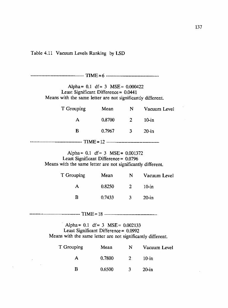
137
Table 4.11 Vacuum Levels Ranking by LSD
TIME-6
Alpha= 0.1 df= 3 MSE= 0.000422Least Significant Difference = 0.0441
Means with the same letter are not significantly different.
T Grouping Mean N Vacuum Level
A 0.8700 2 10-in
B 0.7967 3 20-in
TIME =12
Alpha= 0.1 df= 3 MSE= 0.001372Least Significant Difference = 0.0796
Means with the same letter are not significantly different.
T Grouping Mean N Vacuum Level
A 0.8250 2 10-in
B 0.7433 3 20-in
TIME =18
Alpha= 0.1 df= 3 MSE= 0.002133Least Significant Difference = 0.0992
Means with the same letter are not significantly different.
T Grouping Mean N Vacuum Level
A 0.7800 2 10-in
B 0.6500 3 20-in
138
moisture damage more effectively than climatic extremes of precipitation and
temperature (Lottman, 1971). Although many water sensitivity researchers agree on
the importance of including the traffic variable in any water sensitivity test, most of
them have tried to compromise this variable due to the difficulty of simulation and
the need for costly instrumentation. Repeated loading was selected to simulate
traffic and was combined with two other variables, temperature cycling and water
conditioning. Repeated loading in the ECS is intended to induce part of the
deterioration while the other variables contribute the remainder, unlike the typical
fatigue and rutting test procedures where repeated loading dominates the asphalt
concrete deterioration. Three parameters were considered in selecting the repeated
loading mode; loading level, loading time, and stress-strain condition, which are
discussed as follows:
1-Loading Level
The loading is fixed at 200 lbs (1.0 kN) repeated load with a 60 lbs (0.1 kN) static
load to keep the specimen from rebounding. The selection of loading level was
made after a trial and error process of changing the load level and monitoring total
permanent deformation of the specimen after each conditioning cycle. This loading
level was selected from others, not reported here, to be sufficiently moderate to
minimize permanent deformation. Permanent deformation is monitored by a linear

139
variable differential transducer (LVDT) located at the top of the load cell and
integrated with the signal conditioning unit and personal computer.
2-Loading Time
Although the ECS is capable of providing a variety of frequencies and wave forms,
the ECS uses a square pulse load with a pulse load time of 0.1 s and rest period of
0.9s.
3-Stress-Strain Conditions
Since the ECS uses an electro-pneumatic closed loop system for the repeated loading
subsystem, the ECS tests are conducted under controlled stress conditions which
appear reasonable in light of previous experience. It was necessary to select a
loading level to provide an appropriate traffic simulation without inducing significant
permanent deformation. The main factors affecting the permanent deformation in
this controlled experiment are the loading and air voids levels. Loading level is
discussed above.
In order to measure the entire accumulated permanent deformation of the specimen
during the conditioning cycles, a temporary arrangement for the test setup was used.
In addition to the two original LVDTs, a third LVDT was mounted on top of the
140
load cell. The third LVDT was integrated with the computer program through the
signal conditioning unit to collect the permanent deformation of the specimen during
the conditioning cycle (6 hours) and during the three hours of cooling time to the
testing temperature 25 °C.
To demonstrate the effect of air voids on the permanent deformation, two specimens
were prepared from the same asphalt-aggregate combination, RB/AAG-1, and
compacted at two air voids levels: Specimen RLC58RB/AAG-1 with low (5 percent)
air voids and Specimen RC53RB/AAG-1 with medium (8 percent) air voids.
Figure 4.8 shows the permanent deformation that accumulated under repeated
loading and during three 6-hour hot water conditioning cycles with a 3-hour cooling
period after each hot cycle. Generally, the major permanent deformation took place
during the first conditioning cycle. In addition, the specimens recovered much of the
deformation during the 3-hour cooling time. Moreover, due to differences in
susceptibility to consolidation under repeated loading, the specimen with high air
voids exhibited higher permanent deformation than the specimen with low air voids.
This investigation indicates that 200 lbs repeated loading during water conditioning
cycles is appropriate.
In order to investigate the effect of repeated loading on the deterioration process
( retained MR) during water conditioning, two sets of specimens from the same
asphalt-aggregate mixture with the same air void level were subjected to hot-
saturated water conditioning (code C, Fig. 2.1). One set was water conditioned with
static loading and the second was conditioned with repeated loading.
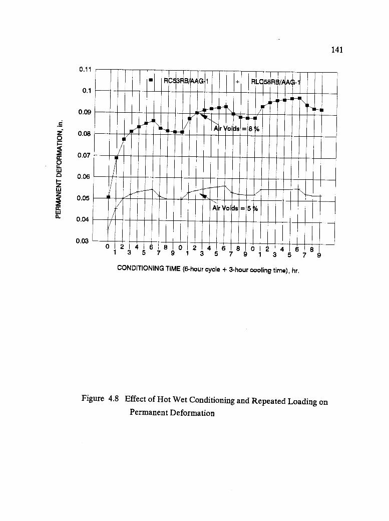
0.11
0.1
0.09
0.08
0.07
0.06
0.05
0.04
0.03
141
R653 RBAAAG.1 + RLC58RB/AAG-1
r Voids 8%
A1r Voids 5%
0 2 4 6 8 0 2 4 6 8 0 2 4 6 81 3 5 7 9 1 3 5 7 9 1 3 5 7 9
CONDITIONING TIME (6-hour cycle + 3-hour cooling time), hr.
Figure 4.8 Effect of Hot Wet Conditioning and Repeated Loading onPermanent Deformation
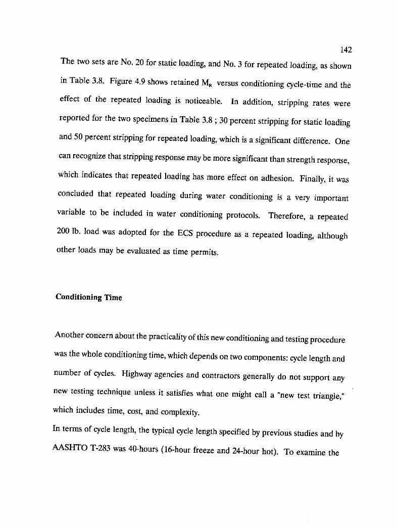
142
The two sets are No. 20 for static loading, and No. 3 for repeated loading, as shown
in Table 3.8. Figure 4.9 shows retained MR versus conditioning cycle-time and the
effect of the repeated loading is noticeable. In addition, stripping rates were
reported for the two specimens in Table 3.8 ; 30 percent stripping for static loading
and 50 percent stripping for repeated loading, which is a significant difference. One
can recognize that stripping response may be more significant than strength response,
which indicates that repeated loading has more effect on adhesion. Finally, it was
concluded that repeated loading during water conditioning is a very important
variable to be included in water conditioning protocols. Therefore, a repeated
200 lb. load was adopted for the ECS procedure as a repeated loading, although
other loads may be evaluated as time permits.
Conditioning Time
Another concern about the practicality of this new conditioning and testing procedure
was the whole conditioning time, which depends on two components: cycle length and
number of cycles. Highway agencies and contractors generally do not support any
new testing technique unless it satisfies what one might call a "new test triangle,"
which includes time, cost, and complexity.
In terms of cycle length, the typical cycle length specified by previous studies and by
AASHTO T-283 was 40-hours (16-hour freeze and 24-hour hot). To examine the
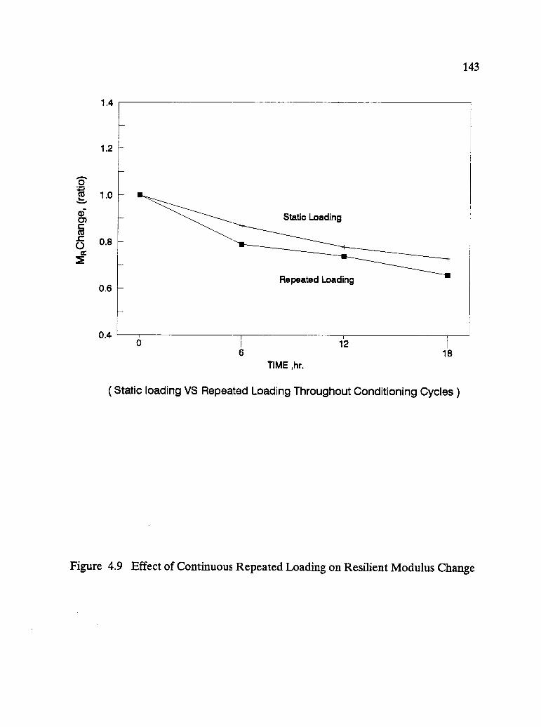
1.4
1.2
1.0
0.8
0.6
0.4
143
Static Loading
Repeated Loading
6
TIME ,hr.
1218
( Static loading VS Repeated Loading Throughout Conditioning Cycles )
Figure 4.9 Effect of Continuous Repeated Loading on Resilient Modulus Change
144
effect of cycle length, two similar sets of specimens were subjected to the same
conditioning code (code C, Fig. 2.1). One set (No. 20) was conditioned for 6-hour
cycles and the second set (No. 23, Table 3.8) was conditioned for 24-hour cycles.
The data of the two sets were plotted in Figure 4.10 and shows only slight difference
between the two cycle lengths after completing 3 cycles. Since the cycling process
contributes more to damage than cycle length, a 6-hour cycle was established for the
ECS water conditioning, either freeze or hot conditioning.
In terms of the number of cycles, it is known that the more the cycles, the closer the
simulation to the field cycling conditions,where the number of cycles representes day-
night and summer-winter cycles. After establishing the cycle length of 6 hours, three
cycles for hot conditioning were proposed, because this is a practical test duration
with considering the expected freezing cycles, which is discussed later. So, after
proposing three cycles, the question was, do the second and third cycles have a
significant effect on the deterioration process? If there is insignificant water damage
after the first cycle, one can end the hot cycles at the end of the first cycle, and the
same thing applies between the second and the third cycles. The question is, if the
second and third cycles do induce more water damage, is it consistent? In other
words, are the three slopes of the three MR ratios (the slopes of the first cycle, first
+ second cycles, and first + second + third cycles) similar? If there is an
insignificant difference between the slopes of the three combinations of the three MR
ratios, one can predict the effect of the second cycle without performing it, and the
same thing applies with the third cycle.
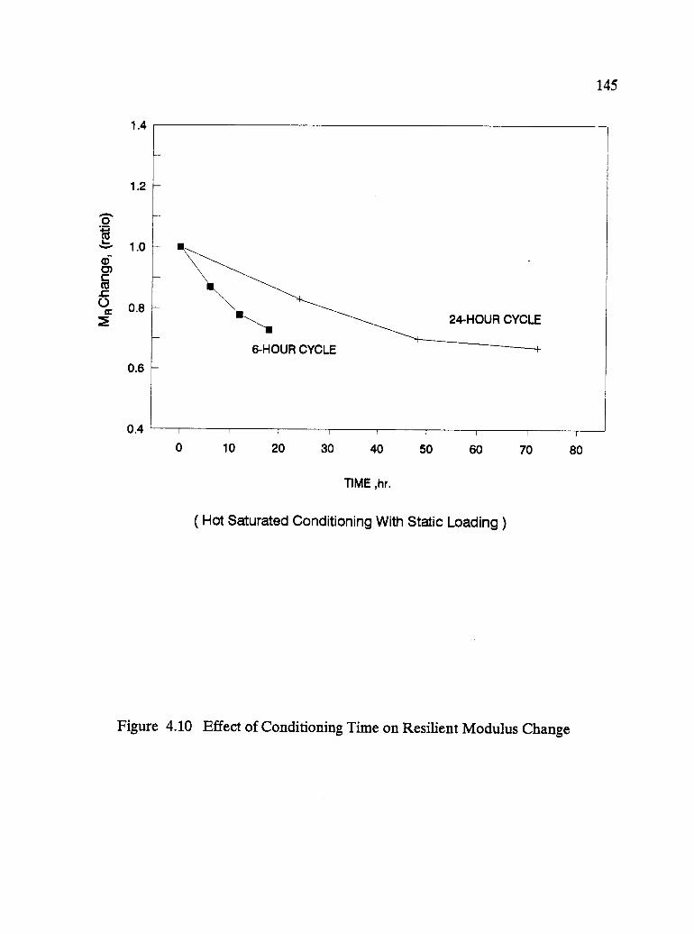
1.4
1.2
1.0
0.8
0.6
0.4
145
0 10 20 30 40
TIME ,hr.
( Hot Saturated Conditioning With Static Loading )
50 60 70 80
Figure 4.10 Effect of Conditioning Time on Resilient Modulus Change
146
In order to answer the two questions, MR ratios of three specimens from the same
combination, which were subjected to three hot-wet cycles with continuous repeated
loading, have been statistically analyzed. The slopes were calculated and shown in
Table 4.12 (the original data were extracted from Table 3.8).
In order to see if there is a significant difference between the three cycles, the MR
ratios were analyzed. The GLM was performed by comparing MR ratios resulting
from the first conditioning cycle to MR ratios resulting from the second and third
conditioning cycles. Table 4.13 includes the GLM results, which showed
a significant difference among the three cycles at the 95 percent confidence level.
Moreover, MR ratios from the three cycles are ranked clearly by LSD analysis at the
90 percent confidence level as shown in Table 4.14. This means that the more
conditioning cycles the more the deterioration.
In order to analyze the differences between the three deterioration trends (slopes,
which was the second question), linear regression analyses were performed to
calculate the three slopes resulting from the three conditioning cycles ( first cycle,
first and second cycles, and first, second, and third cycles), as shown in Table 4.12.
Then the GLM was performed on the slopes of MR ratios of the three specimens.
The statistical analysis, Table 4.15, shows that there are significant differences among
the three slopes at the 95 percent confidence level. Also, the three slopes were
ranked by LSD at the 90 percent confidence level, as shown in Table 4.16. This
comparison indicates that one cannot predict the effect of the second and/or the
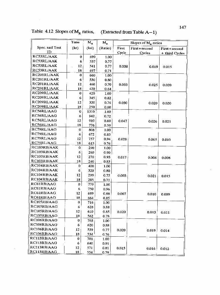
147Table 4.12 Slopes of MR ratios, (Extracted from Table A-1)
Spec. and TestID
Time
(hr)MR
(ksi)MR
(Ratio)Slopes of MR ratios
FirstCycle
First + secondCycles
First + second+ third Cycles
RC53RL/AAK 0 699 1.00RC53RL/AAK 6 537 0.77RC53RL/AAK 12 541 0.77 0.038 0.019 0.015RC53RL/AAK 18 497 0.71RC201RL/AAK 0 660 1.00RC201RL/AAK. 6 530 0.80RC201RL/AAK 12 460 0.70 0.033 0.025 0.020RC201RL/AAK 18 420 0.64RC209RL/AAK 0 420 1.00RC209RL/AAK 6 345 0.82RC209RL/AAK 12 320 0.76 0.030 0.020 0.020RC209RL/AAK 18 250 0.60RC56RL/AAG 0 1310 1.00RC56RL/AAG 6 942 0.72RC56RL/AAG 12 910 0.69 0.047 0.026 0.021RC56RL/AAG 18 776 0.59RC79RL/AAG 0 808 1.00RC79RL/AAG 6 672 0.83RC79RL/AAG 12 757 0.94 0.028 0.005 0.010RC79RL/AAG 18 615 0.76RC103RB/AAK 0 290 1.00RC103RB/AAK 6 260 0.90RC103RB/AAK 12 270 0.93 0.017 0.006 0.008RC103RB/AAK 18 240 0.83RC104RB/AAK 0 400 1.00RC104RB/AAK 6 320 0.80RC104RB/AAK 12 299 0.75 0.003 0.021 0.015RC104RB/AAK 18 285 0.71RC61RB/AAG 0 779 1.00RC61RB/AAG 6 750 0.96RC61RB/AAG 12 689 0.88 0.007 0.010 0.009RC61RB/AAG 18 664 0.85RC105RB/AAG 0 716 1.00RC105RB/AAG 6 628 0.88RC105RB/AAG 12 610 0.85 0.020 0.013 0.011RC105RB/AAG 18 562 0.78RC106RB/AAG 0 703 1.00RC106RB/AAG 6 620 0.88RC106RB/AAG 12 539 0.77 0.020 0.019 0.014RC106RB/AAG 18 534 0.76RC113RB/AAG 0 701 1.00RC113RB/AAG 6 640 0.91RC113RB/AAG 12 571 0.81 0.015 0.016 0.012RC113RB/AAG 18 554 0.79
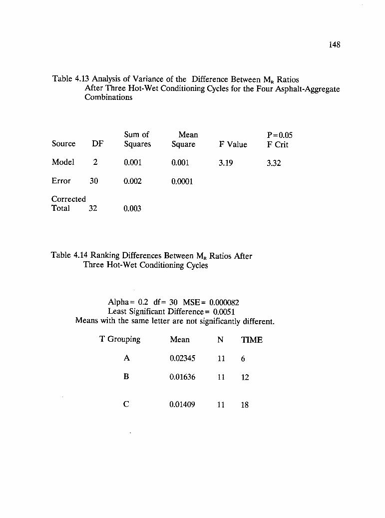
148
Table 4.13 Analysis of Variance of the Difference Between MR RatiosAfter Three Hot-Wet Conditioning Cycles for the Four Asphalt-AggregateCombinations
Sum of Mean P = 0.05Source DF Squares Square F Value F Crit
Model 2 0.001 0.001 3.19 3.32
Error 30 0.002 0.0001
CorrectedTotal 32 0.003
Table 4.14 Ranking Differences Between MR Ratios AfterThree Hot-Wet Conditioning Cycles
Alpha= 0.2 df= 30 MSE= 0.000082Least Significant Difference = 0.0051
Means with the same letter are not significantly different.
T Grouping Mean N TIME
A 0.02345 11 6
B 0.01636 11 12
C 0.01409 11 18
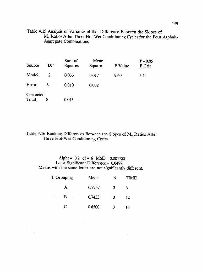
149
Table 4.15 Analysis of Variance of the Difference Between the Slopes ofMR Ratios After Three Hot-Wet Conditioning Cycles for the Four Asphalt-Aggregate Combinations
Sum of Mean P = 0.05Source DF Squares Square F Value F Crit
Model 2 0.033 0.017 9.60 5.14
Error 6 0.010 0.002
CorrectedTotal 8 0.043
Table 4.16 Ranking Differences Between the Slopes of MR Ratios AfterThree Hot-Wet Conditioning Cycles
Alpha= 0.2 df= 6 MSE= 0.001722Least Significant Difference = 0.0488
Means with the same letter are not significantly different.
T Grouping Mean N TIME
A 0.7967 3 6
B 0.7433 3 12
C 0.6500 3 18
150
third cycle from the effect of the first cycle or cycles, within an acceptable confidence
level. In addition to the above reasoning for the need to perform the three cycles,
performing the three cycles increases the confidence level of the test. Although it
does not increase the degrees of freedom (because the slopes are in the same
direction), the results of each cycle confirm the preceding cycles. A later section,
includes an extended discussion with more details about this approuch to developing
the ECS water conditioning procedure.
4.3 Visual Evaluation
Direct observation can provide insight as to the nature and extent of stripping. The
primary disadvantage of visual evaluation of stripping is the subjective nature of the
results. Sometimes, in an attempt to limit the subjectivity of the visual evaluation,
rating patterns are compared to actual specimens to aid the rater and help in
establishing consistency in the results (Field and Phang 1986). Another technique
used to provide insight on the stripping potential of the fine aggregate is use of
a stereo zoom microscope.
A new evaluation technique was developed that includes six levels of rating
patterns, 5, 10, 20, 30, 40, and 50 percent stripping, as shown in Figure 4.11. In
addition, a stereo zoom microscope is used to make it practical and easy to
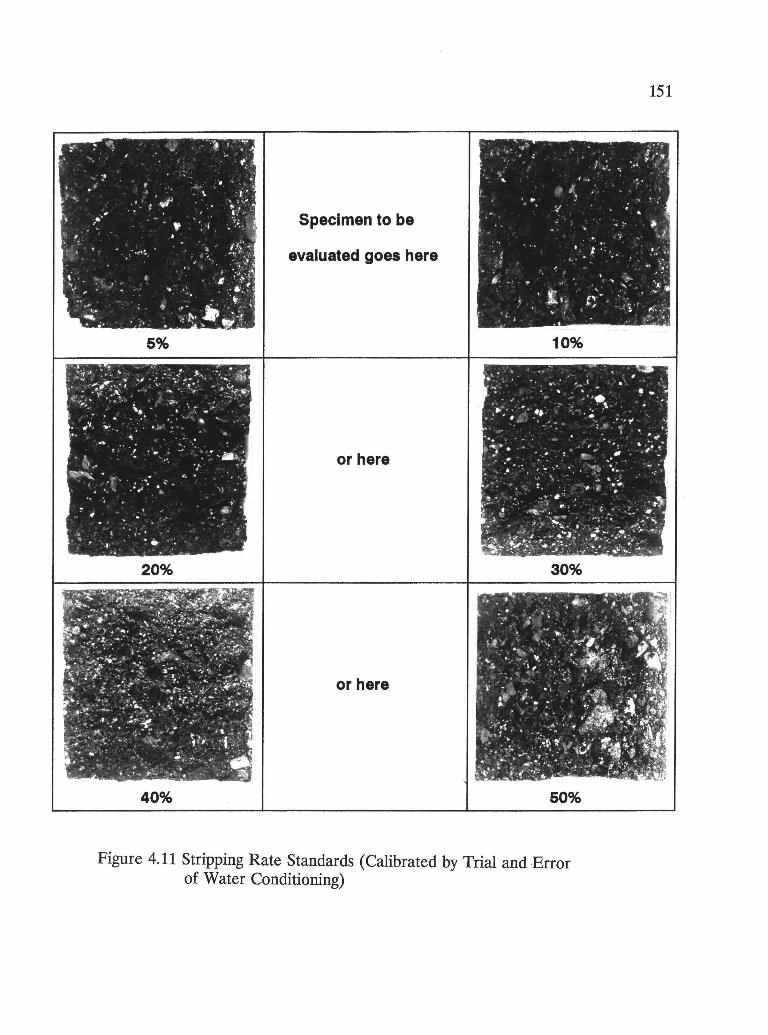
011
0
0
0c.)
00.c16
0U)
0
0
rt:s
Cd
Cd
Cd;-
Cd
7:3
cd
1)c3 CD
b.()
0
r-I
0)
a.
152
distinguish between the detail levels. The standard six levels were established using
compacted asphalt concrete specimens made from a range of aggregate types and
subjected to different water conditioning levels. The fractured interior faces were
adjusted manually to six stripping levels (standards). The six standard specimens are
mounted in a plywood frame with nine (3 x 3) rectangular openings as shown in
Figure 4.11. The three empty slots are used for the tested specimens which are to
be rated.
This new technique has been used on all the ECS conditioned specimens to
date. Following the final resilient modulus test, the specimen was split apart and the
stripping rate was determined. This study was aimed at how engineers might utilize
the visual evaluation and retained mechanical properties (MR) after water
conditioning. Due to space limitations, only one asphalt-aggregate combination,
RB/AAG-1, will be discussed here as an illustration of the procedure.
Five specimens were prepared from the same asphalt-aggregate combination
RB/AAG-1 and compacted to the same air voids level, 8 percent ± 1. Each
specimen was subjected to three 6-hour cycles of one type of different water
conditioning. The five conditioning codes and the five test results are as shown in
Table 4.17.
Figure 4.12 shows the stripping rate for the five conditioning procedures. A
correlation between the severity of the specimen conditioning procedure and the
resulting stripping rate is apparent. The most severe conditioning procedure, which
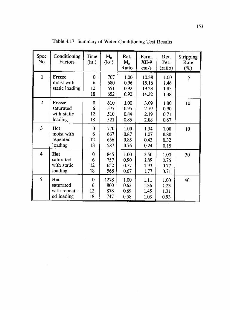
153
Table 4.17 Summary of Water Conditioning Test Results
Spec.No.
ConditioningFactors
Time(hr.)
MR(ksi)
Ret.MR
Ratio
Perm.XE-9cm/s
Ret.Per.
(ratio)
StrippingRate(%)
1 Freeze 0 707 1.00 10.38 1.00 5moist with 6 680 0.96 15.16 1.46static loading 12 651 0.92 19.23 1.85
18 652 0.92 14.32 1.38
2 Freeze 0 610 1.00 3.09 1.00 10saturated 6 577 0.95 2.79 0.90with static 12 510 0.84 2.19 0.71loading 18 521 0.85 2.08 0.67
3 Hot 0 770 1.00 1.34 1.00 10moist with 6 667 0.87 1.07 0.80repeated 12 656 0.85 0.43 0.32loading 18 587 0.76 0.24 0.18
4 Hot 0 845 1.00 2.50 1.00 30saturated 6 757 0.90 1.89 0.76with static 12 652 0.77 1.93 0.77loading 18 568 0.67 1.77 0.71
5 Hot 0 1278 1.00 1.11 1.00 40saturated 6 800 0.63 1.36 1.23with repeat- 12 878 0.69 1.45 1.31ed loading 18 747 0.58 1.03 0.93
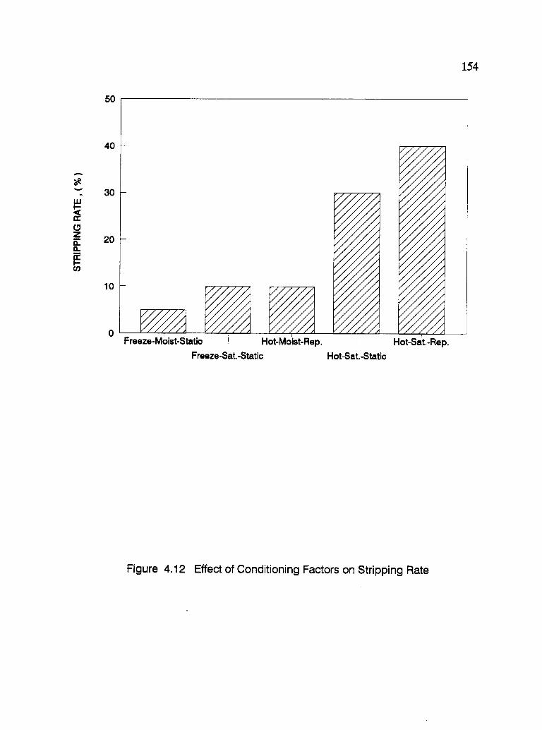
50
40
30
20
10
0
154
Freeze-Moist-Static Hot-Moist-Rep. Hot-Sat.-Rep.
Freeze-Sat.-Static Hot-Sat.-Static
Figure 4.12 Effect of Conditioning Factors on Stripping Rate

155
was three cycles of hot-saturated conditioning with repeated loading (Specimen 5),
induced the highest water damage, 40 percent. On the other hand, a milder
conditioning procedure such as three cycles of freeze-moist conditioning with static
loading (static loading means only holding vacuum level at 10 in. Hg during the
conditioning cycle without repeated axial loading) (Specimen 1) induced the lowest
stripping rate.
As explained earlier, this part of this study attempts to correlate the visual
evaluation method with the mechanical properties of specimens. Therefore, the
retained resilient modulus results after each conditioning cycle, as shown in
Table 4.17 for all the five specimens, were plotted versus the conditioning cycles as
shown in Figure 4.13. In general, the five mixtures are ranked in the same order to
as that determined by visual stripping.
Figure 4.13 shows that hot-saturated conditioning with static loading is more
severe than hot-moist conditioning with repeated loading. This result indicates that
the degree of saturation has a more significant effect than repeated loading on the
water damage process, at least for this mixture. Moreover, a close match between
stripping rates and MR change (by comparing Figure 4.12 with Figure 4.13) indicates
the possibility of using a visual estimate of stripping as part of the evaluation system.
Using only mechanical tests such as MR tends to mask the relative importance of
different mechanisms of water damage, cohesion or adhesion loss, that may occur
simultaneously.
The overall mechanism of stripping is complex and is being studied from
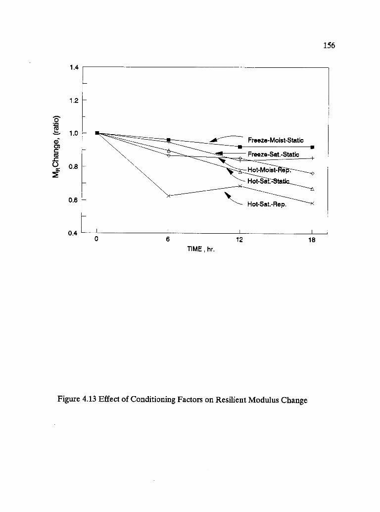
1.4
1.2
1.0
0.8
0.6
0.4
156
0 6
TIME , hr.
12
Figure 4.13 Effect of Conditioning Factors on Resilient Modulus Change
18
157
several points of view within the SHRP program. Adsorption/desorption of asphalt
on aggregate surfaces (see the final report of water sensitivity based on the chemical
and physical bond by Curtis et al., 1992) is a key factor and will most likely play a
role in the emerging new test procedure. Other studies, such as a detailed evaluation
of the size, shape, and distribution of voids in the mixture, may help confirm the
pessimum voids concept (see the study of Void Structure by SHRP, 1992). Still other
ideas include the loss of (dissolving of) aggregate surface minerals as a source or
cause of asphalt stripping. It is expected that the other studies ,i.e., SHRP, will
contribute to the understanding of stripping and needs to be incorporated with this
procedure.
4.4 Permeability
There is a general perception that permeability is a better indicator of mixture
durability than percent air voids because permeability measures fluid accessibility
through the asphalt concrete. Moreover, studies by Hein and Schmidt, 1961, show
that permeability,when induced by mix design changes, is not always proportional to
void content. The permeability and air voids data shown in Table 3.9 is displayed
in Figure 4.14. Figure 4.14 shows that the relationship between permeability and air
voids is not a proportional relationship, especially when the data is obtained from
different asphalt-aggregate combinations. This finding is contrary to customary
conceptions. Early investigators Ellis and Schmidt, 1961, were concerned with

12
11
10
9
8
7
6
5
4
3
2
1
0
158
-4r+++
+
0 5 10 15 20 25 30 35
PERMEABILITY ,K, XE-9 cm/sec
Figure 4.14 Permeability-Air Voids Relationship
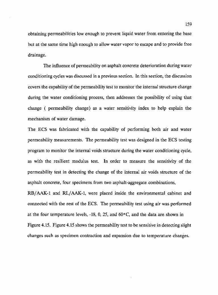
159
obtaining permeabilities low enough to prevent liquid water from entering the base
but at the same time high enough to allow water vapor to escape and to provide free
drainage.
The influence of permeability on asphalt concrete deterioration during water
conditioning cycles was discussed in a previous section. In this section, the discussion
covers the capability of the permeability test to monitor the internal structure change
during the water conditioning process, then addresses the possibility of using that
change ( permeability change) as a water sensitivity index to help explain the
mechanism of water damage.
The ECS was fabricated with the capability of performing both air and water
permeability measurements. The permeability test was designed in the ECS testing
program to monitor the internal voids structure during the water conditioning cycle,
as with the resilient modulus test. In order to measure the sensitivity of the
permeability test in detecting the change of the internal air voids structure of the
asphalt concrete, four specimens from two asphalt-aggregate combinations,
RB/AAK-1 and RL/AAK-1, were placed inside the environmental cabinet and
connected with the rest of the ECS. The permeability test using air was performed
at the four temperature levels, -18, 0, 25, and 60 °C, and the data are shown in
Figure 4.15. Figure 4.15 shows the permeability test to be sensitive in detecting slight
changes such as specimen contraction and expansion due to temperature changes.
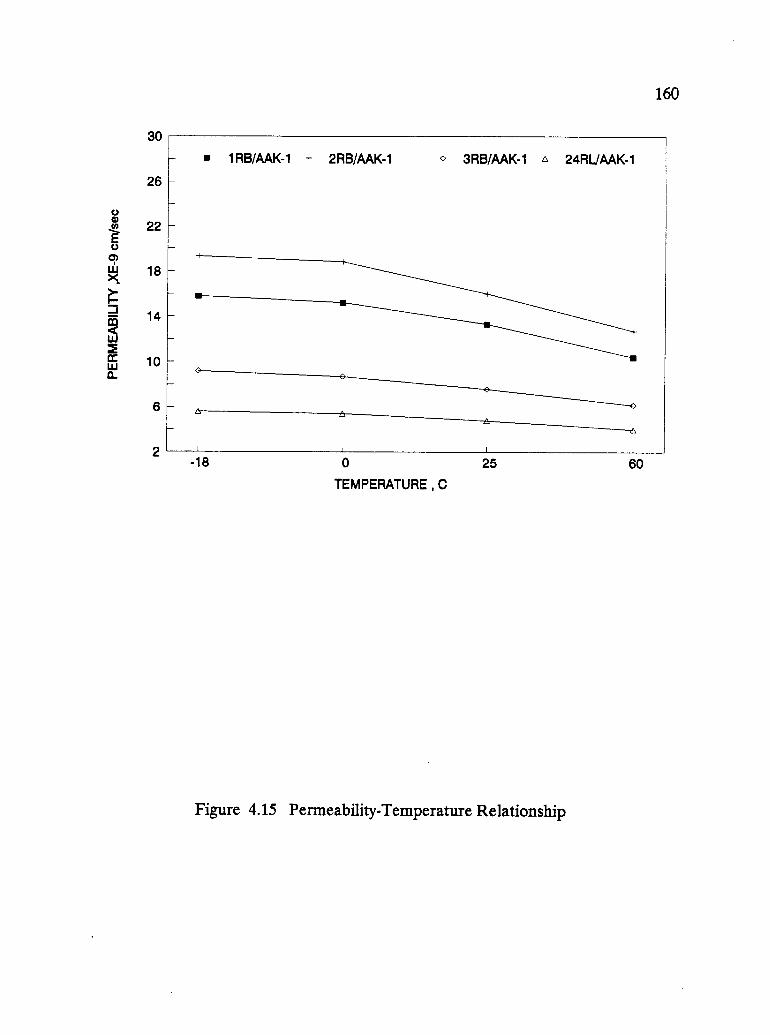
30
26
22
18
14
10
6
2
160
-18 0
TEMPERATURE ,C
25
Figure 4.15 Permeability-Temperature Relationship
60
161
It has been difficult to provide the same reliability using water rather than air for
permeability tests, because permeability is sensitive to the test conditions. The
following conditions must be maintained for the permeability test:
1. Continuity of flow with no volume change.
2. Flow with the voids fully saturated with fluid.
3. Steady state flow with no changes in pressure gradient.
In order to provide a water flow with voids fully saturated with water, a very
high pressure is required. Vallerga and Hicks, 1968, tested water permeability with
50 psi back pressure. The vacuum level used for the ECS procedure is 20-in. Hg,
which is equivalent to only 10 psi. Using higher pressure for ECS water conditioning
was constrained by the desirable maximum 80 percent saturation (partially saturated)
level to reduce the destructive effect of hydrostatic pressure inside the specimen.
In an attempt to provide consistent permeability test results with the available
wetting or saturation levels used in the ECS water conditioning, the water
permeability test (in addition to air permeability which is used for dry specimens)
was conducted on each specimen prior to water conditioning and again after each 6-
hour conditioning cycle. The retained permeability versus conditioning cycles are
plotted for five specimens listed in Table 4.17 and shown in Figure 4.16. The data
show considerable variation in the general trends, especially since all the specimens
were prepared from the same materials combination.

2
1.8
1.6
1.4
1.2
1.0
0.8
0.6
0.4
0.2
0
162
0 6
TIME , hr.
12 18
Figure 4.16 Effect of Conditioning Factors on Permeability Change
163
The results were somewhat unexpected, but indicate that the conditioning procedure
plays an important role in the behavior of mixtures and the void structure. However,
the results appear to be inconsistent with respect to the retained MR (see Figure
4.13). It appears that measuring permeability of partially saturated mixtures is a
major source of the variability.
164
4.5 Confirmation of Hypothesis
As explained in the previous section, the hypothesis of the pessimum voids
concept suggests that the water in the void system of asphalt concrete plays an
important role in its performance. If mixtures of asphalt concrete are water
conditioned, the retained strength is typically lower than the original, unconditioned,
strength. This effect can be characterized by the voids in the mixture. Mixtures with
very low air voids such as 4 percent, where the mixture is almost impermeable to
water, are essentially not affected by water. Mixtures with air voids more than some
critical value, such as 14 percent, do not show significant water damage even though
they are very permeable to water, because there is free drainage and the mixture
does not hold the water for very long. Between these two extremes of impermeable
and free draining mixtures is a range of air voids which is accessible to water, but
lacking free drainage and thus tends to retain water. This range experiences the
highest water damage.
It was necessary to prove the above analogy of the pessimum voids concept
in the laboratory, but the ECS laboratory experiment plan was not appropriate to be
used directly for this purpose. The ECS experiment was designed to simulate field
service conditions in such a way as to accelerate the service conditions by retaining
the water inside the specimen under the effect of vacuum during the conditioning
165
cycles. Free drainage is not provided in this experiment, which is a very important
condition to show the behavior of open graded mixtures in retaining a high ratio of
their original strength after water conditioning.
Another water conditioning study was conducted exclusively to prove the
pessimum voids concept by providing free drainage. A separate conditioning set-up
was constructed to permit this conditioning to simulate the action of free drainage
following wetting. Three 2-specimen sets of mixtures were prepared from the same
asphalt-aggregate combination (RL/AAK) and compacted at three air void contents;
low at 4 percent, pessimum range at 8 percent and free drainage at 30 percent. The
diametral resilient modulus, MR, was then determined for each specimen. The six
specimens were placed in a vacuum container and a partial vacuum of 22 in. Hg was
applied for 10 minutes. Then, the vacuum was removed and the specimens were left
submerged in the water for 30 minutes. This wetting process was selected by trial
and error to provide partial saturation of 70 percent for the specimens with 8 percent
air voids. Using the same procedure, open graded and low air void specimens
resulted in degrees of saturation of 99 and 38 percent, respectively, as shown in
Table 4.18.
The relationship between air voids and level of saturation implies that
specimens with high air voids are totally accessible to water, and in specimens with
very low air voids they are not interconnected and essentially not accessible. The
wetting mechanism of the specimens with 8 percent air voids falls between the two
extremes.
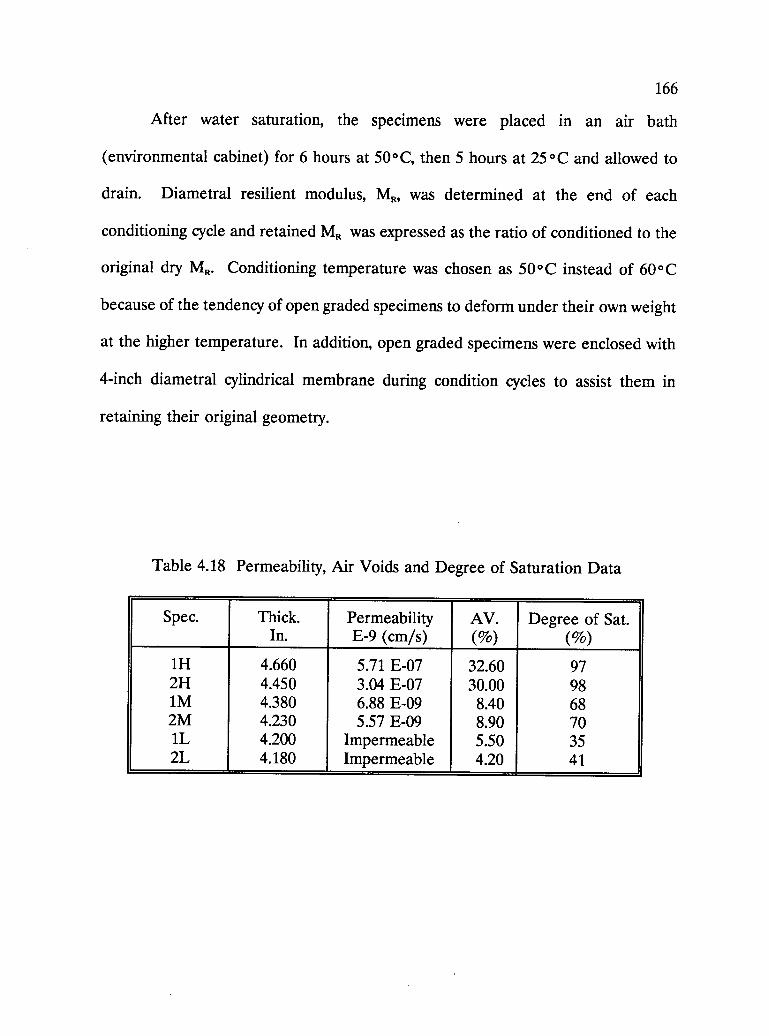
166
After water saturation, the specimens were placed in an air bath
(environmental cabinet) for 6 hours at 50°C, then 5 hours at 25 °C and allowed to
drain. Diametral resilient modulus, MR, was determined at the end of each
conditioning cycle and retained MR was expressed as the ratio of conditioned to the
original dry MR. Conditioning temperature was chosen as 50°C instead of 60°C
because of the tendency of open graded specimens to deform under their own weight
at the higher temperature. In addition, open graded specimens were enclosed with
4-inch diametral cylindrical membrane during condition cycles to assist them in
retaining their original geometry.
Table 4.18 Permeability, Air Voids and Degree of Saturation Data
Spec. Thick.In.
PermeabilityE-9 (cm/s)
AV.(%)
Degree of Sat.(%)
1H 4.660 5.71 E-07 32.60 972H 4.450 3.04 E-07 30.00 981M 4.380 6.88 E-09 8.40 682M 4.230 5.57 E-09 8.90 701L 4.200 Impermeable 5.50 352L 4.180 Impermeable 4.20 41
167
This conditioning process (partial saturation, 6 hours at 50°C, then 5 hours
at 25 °C) was repeated 20 times (cycles). Table 4.19 summarizes the test results,
and Figure 4.17 shows the data and the average curve of retained MR for the
three specimen sets throughout 20 cycles. Each data point is the average of two
specimens. The impermeable set shows no water damage, and the open graded
set shows a slight decrease in retained MR. The set with the middle, or pessimum
range, shows significant water damage. In order to show the behavior
trend, each set is represented by a regression formula (as shown in Figure 4.17).
Specimens with 8 percent air voids are expressed by the regression formula
y = 0.8x"8, which gives R2 = 0.89. Open graded mixture ratios are expressed by
y = 0.8x-"' with R2 = 0.11. Specimens with 4 percent air voids are expressed by a
linear regression, y = 1.0 + x, and because it is almost a horizontal line, R2 is not
applicable, but one can see the low variation around the line.
In order to display the test results in a format similar to that used earlier to
introduce the pessimum voids concept, MR change air void plots Figure 4.17 was
prepared for selected cycles (from number 1 to number 5 and number 19 and 20).
These results confirm the hypothesis that air voids in the pessimum range play an
important role in asphalt concrete performance in the presence of water. Water
retained in these voids during the service life (as represented by water conditioning
cycles) of the pavement would tend to cause more damage than in mixtures with
either more or less voids.
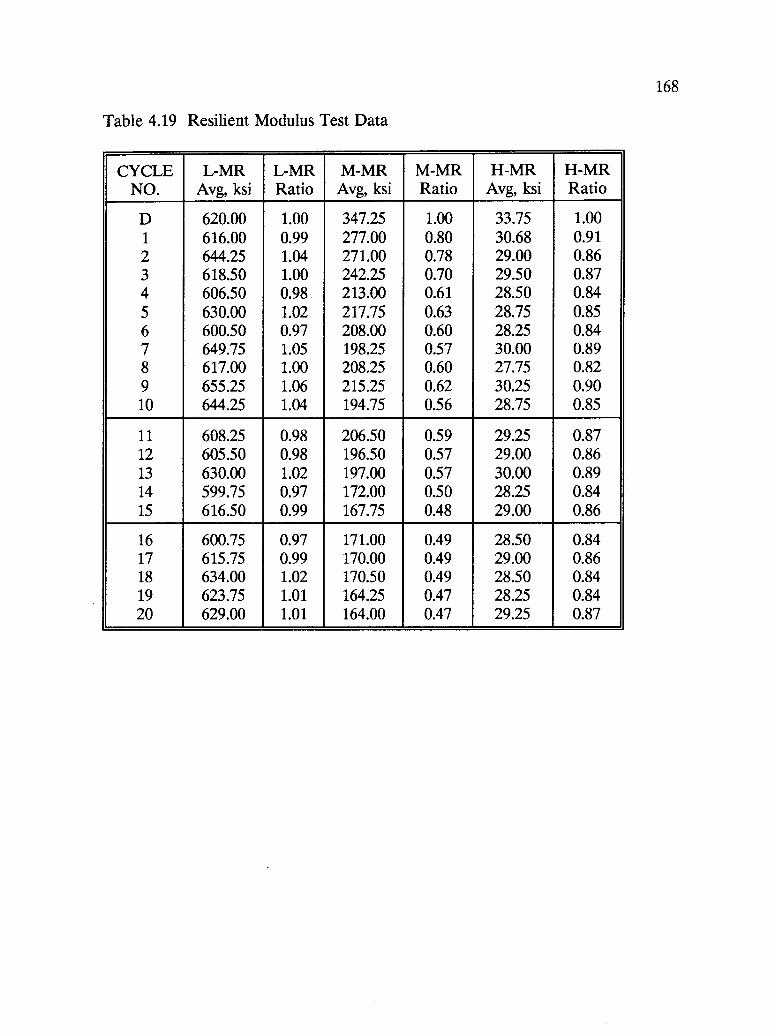
168
Table 4.19 Resilient Modulus Test Data
CYCLENO.
L-MRAvg, ksi
L-MRRatio
M-MRAvg, ksi
M-MRRatio
H-MRAvg, ksi
H-MRRatio
D 620.00 1.00 347.25 1.00 33.75 1.001 616.00 0.99 277.00 0.80 30.68 0.912 644.25 1.04 271.00 0.78 29.00 0.863 618.50 1.00 242.25 0.70 29.50 0.874 606.50 0.98 213.00 0.61 28.50 0.845 630.00 1.02 217.75 0.63 28.75 0.856 600.50 0.97 208.00 0.60 28.25 0.847 649.75 1.05 198.25 0.57 30.00 0.898 617.00 1.00 208.25 0.60 27.75 0.829 655.25 1.06 215.25 0.62 30.25 0.9010 644.25 1.04 194.75 0.56 28.75 0.85
11 608.25 0.98 206.50 0.59 29.25 0.8712 605.50 0.98 196.50 0.57 29.00 0.8613 630.00 1.02 197.00 0.57 30.00 0.8914 599.75 0.97 172.00 0.50 28.25 0.8415 616.50 0.99 167.75 0.48 29.00 0.86
16 600.75 0.97 171.00 0.49 28.50 0.8417 615.75 0.99 170.00 0.49 29.00 0.8618 634.00 1.02 170.50 0.49 28.50 0.8419 623.75 1.01 164.25 0.47 28.25 0.8420 629.00 1.01 164.00 0.47 29.25 0.87
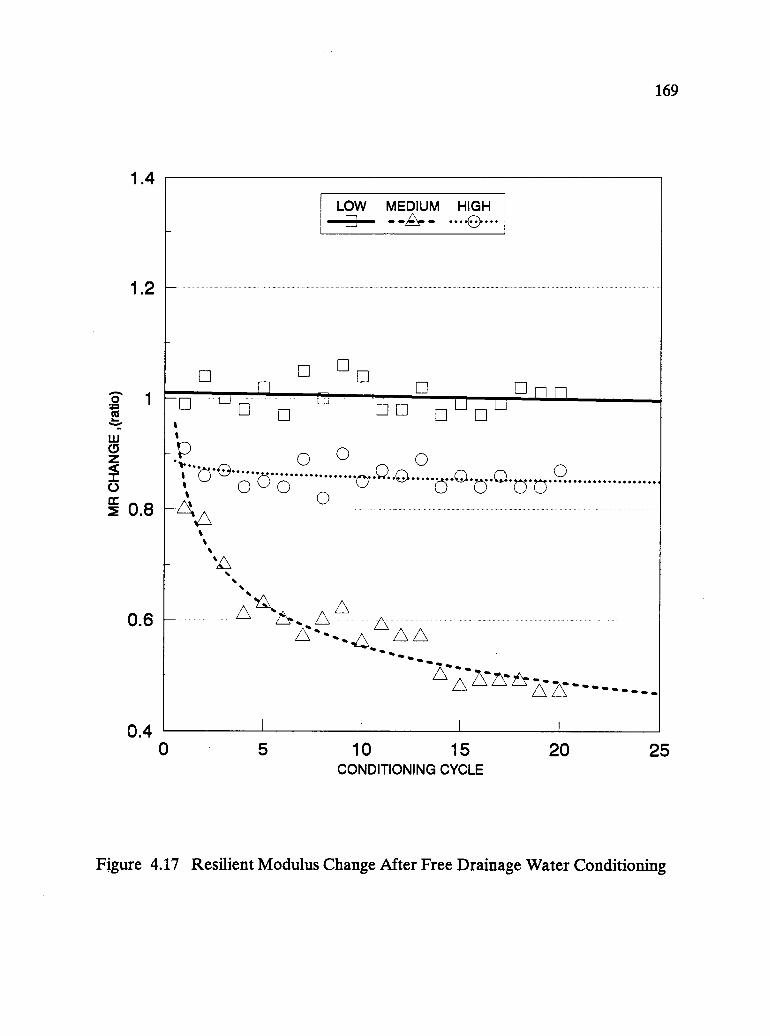
1.4
1.2
169
LOW MEDIUM HIGH- -A- - 0 -
o
0.6
0.40
0
00O
a
0 7 7
A `f\,AAAA
. a .n1
5 10 15CONDITIONING CYCLE
20 25
Figure 4.17 Resilient Modulus Change After Free Drainage Water Conditioning
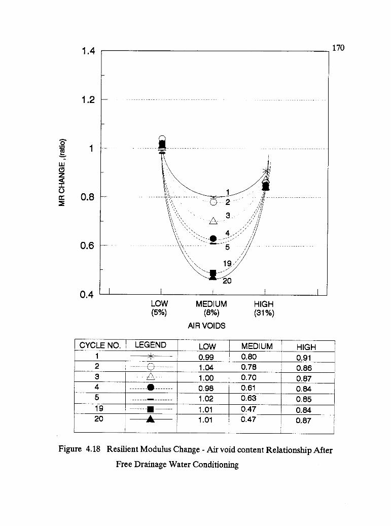
1.4
1.2
0.8
0.6
0.4 1
LOW(5%)
1
MEDIUM HIGH(8%) (31%)
AIR VOIDS
170
CYCLE NO. LEGEND LOW MEDIUM HIGH1 0.99 0.80 0.91x2 1.04 0.78 0.863 1.00 0.70 0.874 0.98 0.61 0.845 1.02 0.63 0.8519 1.01 0.47 0.8420 1.01 0.47 0.87
Figure 4.18 Resilient Modulus Change - Air void content Relationship After
Free Drainage Water Conditioning
171
4.6 Repeatability of the ECS
In the preceding section it has been shown that the test procedure was subjected to
a screening process in order to establish the proper degree of control and field
simulation over the conditioning factors. This has been accomplished by evaluating
the effect of each conditioning variable. Once the development stage was successfully
completed, it was necessary to provide a preliminary overview of the repeatability of
the ECS as a test system and as a test procedure.
Repeatability is a term used to refer to the test result variability associated with a
limited set of specifically defined sources of variability within a single laboratory,
ASTM E 456. A major advantage of the ECS is its ability to serve as both a
conditioning and a testing device at the same time, where all the tests are performed
on the same conditioning setup. As a result of this integration, a test determination
may be described as :
1) value obtained at the end of the ECS-MR test to reflect the
repeatability of the test system, and
2) value obtained at the end of the water conditioning procedure to
represent the repeatability of the conditioning procedure.
172
The repeatability of each value is explained in the following paragraphs.
Test System Repeatability
Although the repeatability of ECS-MR with different test settings is discussed in a
previous section, it is repeated here exclusively with one test setting, which represents
the actual process of the ECS to give a complete picture of the test system. There
are several statistical techniques to describe the variability associated with the test
performance. Coefficient of Variation (CV) is used herein because it is simple and
statistical terms are avoided to the greatest extent. Coefficient of Variation expresses
the standard variation (s) as a percentage of data mean (x), CV = 100 (s/x), (Mandel,
1964).
Two dry specimens were tested for ECS-MR, for one test setting and repeating the
test seven times, i.e., 7 test replicates. The test results as shown in Table 4.20 are
very repeatable with Coefficients of Variation (CV) for the two specimens of 0.9 and
0.6. Such low CVs show the high consistency of the ECS. Since the graphs are
generally useful in visualizing the statistical conclusions, the test results are shown
in Figure 4.19. The test results of each specimen make almost a straight line which
confirmed the above conclusion.
Since the ECS is an automated control, close loop system, the variation indicated by
this analysis expresses only the variation of the test system performance
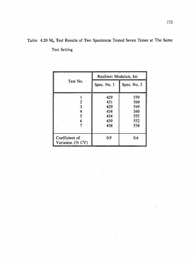
173
Table 4.20 MR Test Results of Two Specimens Tested Seven Times at The Same
Test Setting
Test No.Resilient Moduluis, ksi
Spec. No. 1 Spec. No. 2
1 429 5592 431 5603 429 5494 434 5605 434 5556 439 5527 438 558
Coefficient of 0.9 0.6Variation (% CV)

800
700
600
500
400
300
200
174
Specimen no. 1 + Specimen no. 2
1
23
4Test no.
Figure 4.19 Repeatability ofECS-MR Test
56
7

175
and excludes the variation associated with the conditioning variables and specimen
properties such as air voids and strength.
Repeatability of Water Conditioning Procedure
This section is intended to provide a preliminary overview for the repeatability of the
conditioning evaluation procedure. Although this technique evaluates an asphalt
aggregate mixture response to a water conditioning procedure by using three indices:
resilient modulus change, stripping rate, and permeability change, only resilient
modulus change( MR ratio ) will be discussed in this analysis. MR change is the major
index to monitor the deterioration process during the water conditioning cycles, while
stripping rate is a subjective evaluation which is not as applicable with the
conventional statistical methods. Also, the repeatability of permeability change will
be discussed in the validation report where more data is available. The repeatability
of the test system which was discussed earlier, by analyzing MR test results using the
same measuring process conducted on the same dry specimens provided the simplest
case of the general problem of the adjustment of observations. A more complicated
case arises here, where the retained MR at the end of the conditioning procedure is
derived from combined test values by dividing the conditioning MR by the original dry
MR. In addition to the complexity associated with this test method, there is another
difficulty related to the limited number of test replicates used for the ECS developing
176
program. Fewer replicates were used, because the ECS development testing
evaluated a wide range of variables. Moreover, there are several variables
contributing to the variation of the final retained MR, which can be summarized as:
. Effect of conditioning time,
. Mixture properties, i.e. air voids, strength, and permeability,
. Effect of water by introducing a hydrostatic pressure,
. Temperature cycling,
. Conditioning variables, i.e. repeated loading.
Because of the wide range of variables, a compromise was made in order to decrease
the sources of variability. So the repeatability was analyzed for the MR ratio after
each conditioning cycle rather than representing the whole conditioning procedure
by one MR ratio value. Only the Hot Water Conditioning Procedure, three hot cycles
with repeated loading, is included in this analysis because it was conducted on two
asphalt/aggregate combinations with enough specimen replicates. The data used for
this analysis was extracted from the experiment test plan (Table 3.9) and RL/AAK-1
and RB/AAG-1 combinations were tested for three and four specimen replicates,
respectively. Coefficient of Variation was calculated for each cycle for the same
asphalt/aggregate combination, as shown in Table 4.21. The data exhibit very good
repeatability where CVs were less than 10 percent for the two combinations with
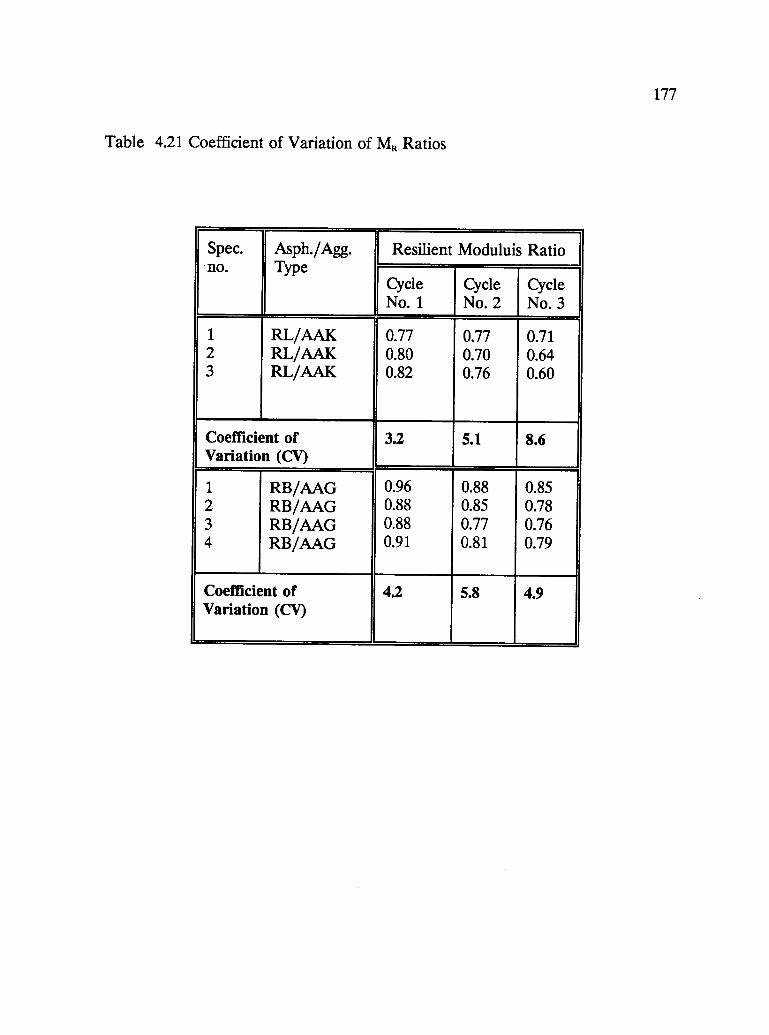
177
Table 4.21 Coefficient of Variation of MR Ratios
Spec.no.
Asph./Agg.Type
Resilient Moduluis Ratio
CycleNo. 1
CycleNo. 2
CycleNo. 3
1
23
RL/AAKRL/AAKRL/AAK
0.770.800.82
0.770.700.76
0.710.640.60
Coefficient ofVariation (CV)
3.2 5.1 8.6
1
234
RB/AAGRB/AAGRB/AAGRB/AAG
0.960.880.880.91
0.880.850.770.81
0.850.780.760.79
Coefficient ofVariation (CV)
4.2 5.8 4.9
178
each cycle. It was preferred to express the repeatability of the conditioning by one
CV value. But since it is not possible to pool coefficients of variation in the same
manner as variances and standard deviations, the simple arithmetic average of the
six CV values was used (ASTM C 802) which is 5.3 percent. In order to display MR
ratios, Figure 4.20 was prepared for the two asphalt/aggregate combinations and
confirms the above conclusion where the variation of MR ratios for each conditioning
is quite reasonable. Interestingly, one can see from CV analysis and Figure 4.20, that
the test variation is not dependant on the number of conditioning cycles. In other
words, CV increases with increasing cycles for the RL/AAK combination ( 3.2, 5.1
and 8.6, in Table 4.21 ), while no trend can be drawn for RB/AAG combination (
4.2, 5.8 and 4.9 ).
If a more sophisticated technique is desired to express the repeatability of the water
conditioning procedure, the appropriate one is the ASTM standard repeatability
index, as explained in ASTM E 456. In order to obtain a quantitative estimate of
repeatability, the standard deviation was calculated for the same MR ratios in
Table 4.21, as shown in Table 4.22. The repeatability estimate may be referred to as
sr, and the formula of a specific estimate is :
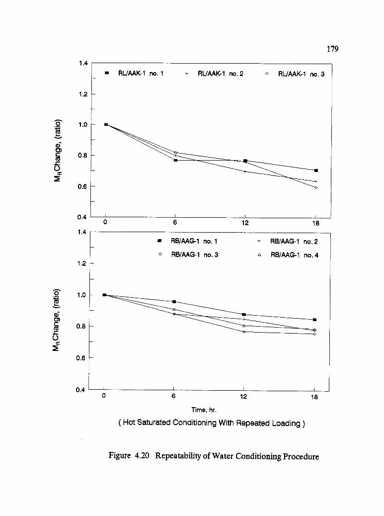
1.4
1.2
1.0
0.8
0.6
0.4
1.4
1.2
1.0
0.8
0.6
0.4
179
0 6 12 18
0 6 12
Time, hr.
( Hot Saturated Conditioning With Repeated Loading )
18
Figure 4.20 Repeatability of Water Conditioning Procedure
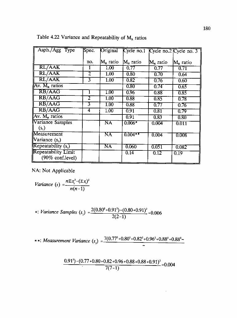
180
Table 4.22 Variance and Repeatability of MR ratios
Asph./Agg Type Spec.
no.
Original
MR ratio
Cycle no.1
MR ratio
Cycle no.2
MR ratio
Cycle no. 3
MR ratioRL/AAK 1 1.00 0.77 0.77 0.71RL/AAK 2 1.00 0.80 0.70 0.64RL/AAK 3 1.00 0.82 0.76 0.60
Av. MR ratios 0.80 0.74 0.65RB/AAG 1 1.00 0.96 0.88 0.85RB/AAG 2 1.00 0.88 0.85 0.78RB/AAG 3 1.00 0.88 0.77 0.76RB/AAG 4 1.00 0.91 0.81 0.79
Av. MR ratios 0.91 0.83 0.80Variance Samples
(si)NA 0.006* 0.004 0.011
MeasurementVariance (s2)
NA 0.004** 0.004 0.008
Repeatability (sr) NA 0.060 0.051 0.082Repeatability Limit
(90% conf.level)0.14 0.12 0.19
NA: Not Applicable
Variance (s) -nEx2--(Ex)2n(n-1)
*: Variance Samples (si) = 2(0.802 +0.912)- (0.80 +0.91)2 =0.0062(2-1)
* *: Measurement Variance (s2) = 7(0.772+0.802+0.822+0.962+0.882+0.882-
0.912) -(0.77 +0.80 +0.82 +0.96 +0.88 +0.88 +0.91)2.0.004
7(7 -1)
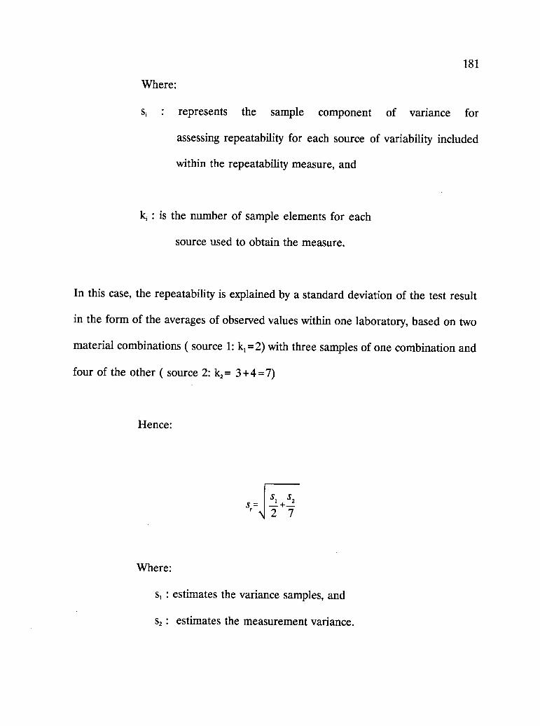
181
Where:
s, represents the sample component of variance for
assessing repeatability for each source of variability included
within the repeatability measure, and
: is the number of sample elements for each
source used to obtain the measure.
In this case, the repeatability is explained by a standard deviation of the test result
in the form of the averages of observed values within one laboratory, based on two
material combinations ( source 1: k1 =2) with three samples of one combination and
four of the other ( source 2: k2 = 3 +4 =7)
Hence:
SrS1 S2- -2 7
Where:
s, : estimates the variance samples, and
s2 : estimates the measurement variance.

182
Based on the data shown in Table 4.22, the estimated repeatability for cycle no. 1 is:
0.006 0 004+ -0.060
2 7
The repeatability ( sr ) values of the other cycles are shown in Table 4.22. All the
values indicate the high repeatability associated with the ECS procedure, which
confirms the conclusion that was derived from the Coefficient of Variation analysis,
above.
When the conditioning procedure is subject only to the type of variability specified
above , the probability of the largest difference between two MR ratios can be
estimated by what is known as a "repeatability limit." Ninety percent repeatability
limit is approximated by 1.65 1r2 sr, (ASTM E 456). It is essential to base this formula
on the estimate that the standard deviation sr derived from a normal distribution.
Accordingly: the 95% repeatability limit = 1.65 v2 s, = 1.65 v2 0.061 = 0.14
The repeatability limits of the other conditioning cycles are shown in Table 4.22. All
the limits fall in a range less than 0.19, (0.14, 0.13, 0.19 ) which indicates a
consistency lower than the one has been concluded earlier from the CV analysis. The
183
variation between the two conclusions, CV and Variance analysis, results from the
fact that the variance analysis is highly dependent on the degree of freedom ( which
is too low here ) on evaluating the variation between the test results.
Although the above conclusion (based on data to date) appears warranted, it should
be noted that this is based only on the development phase data and that the above
conclusions should be regarded as tentative.
In addition to the repeatability, further studies and applications will help in
establishing the reproducibility of the new conditioning procedure by using data from
different laboratories. Reproducibility means test result variability associated with
specifically defined components of variance obtained both from within a single
laboratory and between laboratories, (ASTM E 456). Then the reproducibility will
be used for estimating a statement of precision, because such a statement needs data
from at least six laboratories and at least three materials, (ASTM E 177).

184
4.7 Water Conditioning Procedure
From the previous analysis, water conditioning factors have been established as
follows:
Conditioning temperature; hot conditioning, 60 °C; freeze
conditioning, -18 ° C.
Vacuum level; 20 in. Hg for wetting stage and 10 in. Hg during
the conditioning process.
Cycle length; 6 hours
Conditioning fluid: distilled water
Repeated loading during hot conditioning cycles: a square pulse
load with a pulse load duration of 0.1 s, a pulse load frequency
of 1 HZ, and a pulse load magnitude of 200 lb.
During the development of the ECS conditioning procedure, three aspects
were carefully considered: simulation of service conditions, repeatability and
reproducibility of the test results, and practicality of the test procedure. Service
conditions were established in this test procedure after a detailed investigation of the
effect of each variable, as discussed earlier. The repeatability and reproducibility was
determined after performing a statistical analysis of the test results, and is discussed
in the preceding section. The practicality of the test procedure was one of the major
aspects in the mind of the researcher during the development process, which is
185
discussed in this section. Since the test procedure was mostly automated by the ECS,
the potential simplification was in the test duration and the number of specimens
needed for a complete test. One freezing cycle was considered to be sufficient to
account for the modest effect of cold climate, as discussed earlier, and to provide
simulation for regions that have cold climates. This consideration resulted in two
conditioning procedures; 1) warm climate conditioning procedure which would
include only hot conditioning cycles; 2) cold climate conditioning procedure which
would include hot conditioning cycles and one freeze cycle.
In order to investigate the possibility of conducting the two climate
conditioning procedures on one specimen (dual procedure), two requirements needed
to be satisfied:
1) The effect of freeze cycles should be moderate.
2) There is no effect for climate sequences i.e., no difference between
hot-freeze and freeze-hot cycles.
As discussed earlier, ECS test results confirmed that the effect of freezing cycles is
not significant, which satisfies the first requirement. The second requirement was
investigated by conducting two cycles of hot-freeze conditioning procedure in two
orders, hot-freeze and freeze-hot, as shown in Figure 4.21. Four specimens were
prepared from the same asphalt-aggregate combination and compacted to the same
air void target, 8 percent. The four specimens were divided into two sets, and each

186
a: Hot-Freeze Sequence
CONDITIONING FACTORCONDITIONING STAGE
*WETTING CYCLE-1 CYCLE-2
Vacuum Level (in. Hg) :20 10 10
Repeated Loading NO YS NO
Ambient Temp.(C) ** 25 60 -18
Duration ( hr.) 0.5 6 6
b: Freeze-Hot Sequence
CONDITIONING FACTORCONDITIONING STAGE
*WETTING CYCLE-1 CYCLE-2
Vacuum Level (in. Hg) :20 10 10
Repeated Loading NO NO YS
Ambient Temp.(C) ** 25 -18 60
Duration ( hr.) 0.5 6 6
WETTING : Wetting the Specimen Prior to Conditioning Cycles- Inside the Environmental Cabinet
Figure 4.21 Conditioning Information Charts for Climate Sequence Investigation
187
set was conditioned in different sequence. Figure 4.22 shows the plots of the
averages of MR ratios of two specimens. The difference between the final MR ratios
for the two orders, as shown graphically, is not significant. This confirms that there
is no significant effect of the sequence of the conditioning procedure on MR change.
Based on this finding, it would be possible to perform the freezing cycle at the end
of the hot conditioning procedure. This provides the "dual" conditioning procedure,
which can be performed on one specimen. For example, if the mix design is for a
warm climate region, one can stop at the end of the hot conditioning procedure, and
if the mix design is for a cold climate region one freeze cycle on the same specimen
can be added after performing the hot conditioning procedure.
In the previous section, it was found statistically that the more hot cycles, the
more water damage, and also it was found that the difference between the slope
combinations of three hot cycles ( first cycle, first + second cycle, and first + second
+ third cycles) is statistically significant, which indicates that the deterioration from
the second cycle cannot be predicted by using a regression equation from the first
cycle, and the same thing with the third cycle. Since one freeze cycle was found to
be appropriate at the end of the hot conditioning cycles for cold climate, it was
necessary to investigate the possibility of shorter conditioning procedure and
retaining the freeze conditioning cycle at the end. For this purpose, a separate study
was conducted by investigating three conditioning procedures, as shown in Figure
4.23. The three procedures are; one hot cycle, two hot cycles, and

1.4
1.2
1.0
0.8
0.6
0.4
188
0 6 12
TIME, hr.
(Freeze-Hot or Hot-Freeze)
18 24
Figure 4.22 Effect of conditioning sequence on Resilient Modulus change
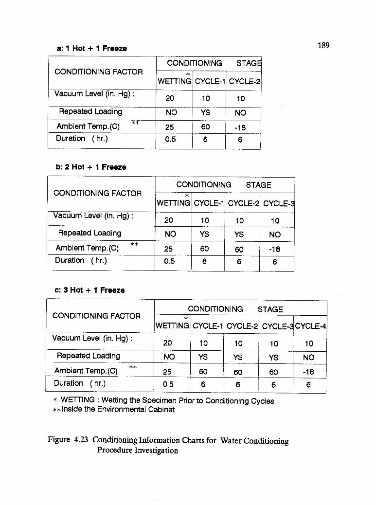
a: 1 Hot + 1 Freeze
CONDITIONING FACTORCONDITIONING STAGE
WETTING CYCLE-1 CYCLE-2
Vacuum Level (in. Hg) :20 10 10
Repeated Loading NO YS NO
Ambient Temp.(C) ** 25 60 -18
Duration ( hr.) 0.5 6 6
b: 2 Hot + 1 Freeze
CONDITIONING FACTORCONDITIONING STAGE
*WETTING CYCLE-1 CYCLE-2 CYCLE-3
Vacuum Level (in. Hg) :20 10 10 10
Repeated Loading NO YS YS NO
Ambient Temp.(C) ** 25 60 60 -18
Duration ( hr.) 0.5 6 6 6
c: 3 Hot + 1 Freeze
189
CONDITIONING FACTORCONDITIONING STAGE
*WETTING CYCLE-1 CYCLE-2 CYCLE-3 CYCLE-4
Vacuum Level (in. Hg) :20 10 10 10 10
Repeated Loading NO YS YS YS NO
Ambient Temp.(C) ** 25 60 60 60 -18
Duration ( hr.) 0.5 6 6 6 6
* WETTING : Wetting the Specimen Prior to Conditioning Cycles**Inside the Environmental Cabinet
Figure 4.23 Conditioning Information Charts for Water ConditioningProcedure Investigation
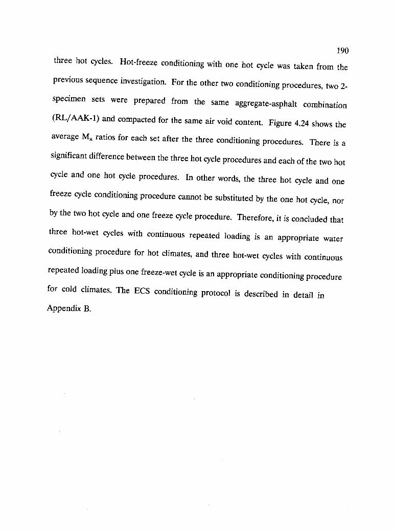
190three hot cycles. Hot-freeze conditioning with one hot cycle was taken from the
previous sequence investigation. For the other two conditioning procedures, two 2-
specimen sets were prepared from the same aggregate-asphalt combination
(RL /AAK -1) and compacted for the same air void content. Figure 4.24 shows the
average M}, ratios for each set after the three conditioning procedures. There is a
significant difference between the three hot cycle procedures and each of the two hot
cycle and one hot cycle procedures. In other words, the three hot cycle and one
freeze cycle conditioning procedure cannot be substituted by the one hot cycle, nor
by the two hot cycle and one freeze cycle procedure. Therefore, it is concluded that
three hot-wet cycles with continuous repeated loading is an appropriate water
conditioning procedure for hot climates, and three hot-wet cycles with continuous
repeated loading plus one freeze-wet cycle is an appropriate conditioning procedure
for cold climates. The ECS conditioning protocol is described in detail in
Appendix B.
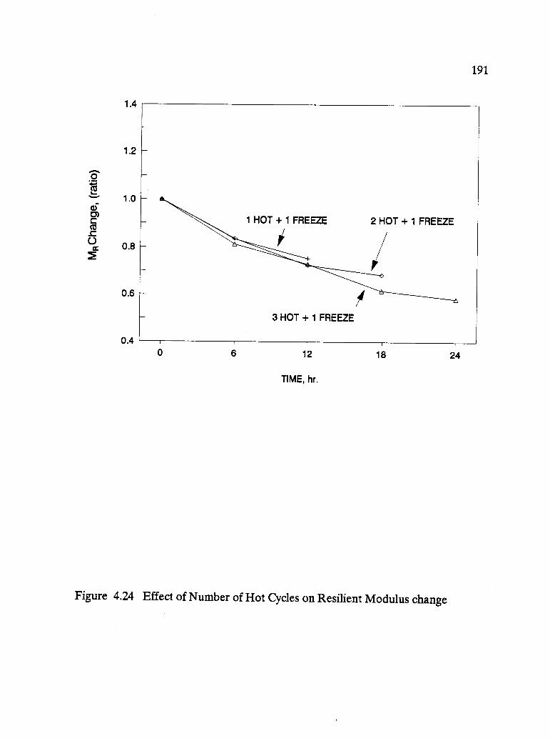
1.4
1.2
1.0
0.8
0.6
0.4
191
0 6 12
TIME, hr.
18
Figure 4.24 Effect of Number of Hot Cycles on Resilient Modulus change
24

192
4.8 AASHTO T-283: Resistance of Compacted Bituminous Mixtures
to Moisture-Induced Damage
Several different tests are used to determine the moisture sensitivity of an asphalt
mixture. AASHTO T-283, including its various improvements is the best known test
procedure among the highway agencies. AASHTO T-283 was used in this study as
a benchmark for comparison. More than one hundred specimens were prepared and
tested for evaluation. For each test, six specimens were divided into two sets (dry
and conditioned sets). Internal water pressure in the conditioned specimens was
produced by vacuum saturation followed by a freeze and thaw cycle. Two numerical
indices of retained resilient modulus (MR) and indirect tensile strength (TS) are
obtained by comparing the retained indirect tensile strength and resilient modulus
of conditioned laboratory specimens with the similar tests of dry specimens.
Table 4.23 summarizes the test data shown in Table 3.2. Retained MR results after
water conditioning for the four asphalt-aggregate combinations are displayed
graphically in Figure 4.25. The data show a significant variation within each
combination, such as that one combination (RB/AK-1) showed MR ratios varying
between 0.60 and 1.12 (Table 4.23), which is unexpectedly high. Likewise, retained
ST results after water conditioning are shown in Figure 4.26. Also, ST ratios

193
Table 4.23 Summary of AASHTO T 283 Water Conditioning Test Results
Test No.Asp h/Agg
CombinationST *
RatioMR *Ratio
1 RL/AAK1 0.54 0.74
2 RL/AAK1 0.6 0.823 RL/AAK1 0.83 0.624 RL/AAK1 0.53 0.535 RL/AAK1 0.93 0.686 RL/AAK1 0.3 0.26
Coefficient of Variation 36.5 32.51 RL/AAG1 0.49 0.402 RL/AAG1 0.3 0.403 RL/AAG1 0.57 0.63
4 RL/AAG1 0.61 0.475 RL/AAG1 0.53 0.606 RL/AAG1 0.4 0.387 RL/AAG1 0.43 0.69
Coefficient of Variation 16 24.51 RB/AAK1 0.64 0.602 RB/AAK1 0.65 0.613 RB/AAK1 0.81 0.724 RB/AAK1 0.67 1.12
5 RB/AAK1 0.79 0.93Coefficient of Variation 11.4 28.2
1 RB /AAG1 1.24 0.622 RB/AAG1 1.16 0.833 RB/AAG1 0.58 0.774 RB/AAG1 0.51 0.625 RB/AAG1 0.77 0.55
Coefficient of Variation 39.1 17.2
Each ST ratio or MR ratio is an average of three test replicates resulting fromdividing MR or ST results of three conditioned specimens by dry MR or STresults of three dry specimens (See Table 3.2 for More Details)

1.4
1.2
1.0
0.8
0.6
0.4
0.2
0
194
+ RL/AAK1 0 RB/AAK1
RLJAAG1 A RB/AAG1
0
0
0
A
2 4
Test replicate
66
Figure 4.25 Resilient Modulus Change After AASHTO T 283 Test
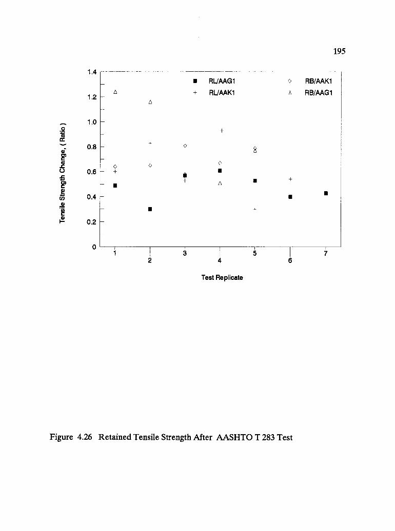
1.4
1.2
1.0
0.8
0.6
0.4
0.2
195
A
o+
A
+
o
RL/AAG1
+ RL/AAK1
o
+
o
8
+
o RB/AAK1
I RB/AAG1
+
1 34
Test Replicate
5
Figure 4.26 Retained Tensile Strength After AASHTO T 283 Test
7
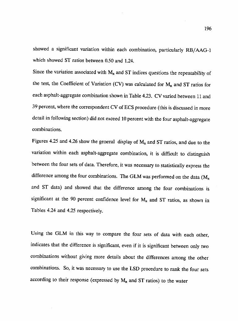
196
showed a significant variation within each combination, particularly RB/AAG-1
which showed ST ratios between 0.50 and 1.24.
Since the variation associated with MR and ST indices questions the repeatability of
the test, the Coefficient of Variation (CV) was calculated for MR and ST ratios for
each asphalt-aggregate combination shown in Table 4.23. CV varied between 11 and
39 percent, where the correspondent CV of ECS procedure (this is discussed in more
detail in following section) did not exceed 10 percent with the four asphalt-aggregate
combinations.
Figures 4.25 and 4.26 show the general display of MR and ST ratios, and due to the
variation within each asphalt-aggregate combination, it is difficult to distinguish
between the four sets of data. Therefore, it was necessary to statistically express the
difference among the four combinations. The GLM was performed on the data (MR
and ST data) and showed that the difference among the four combinations is
significant at the 90 percent confidence level for MR and ST ratios, as shown in
Tables 4.24 and 4.25 respectively.
Using the GLM in this way to compare the four sets of data with each other,
indicates that the difference is significant, even if it is significant between only two
combinations without giving more details about the differences among the other
combinations. So, it was necessary to use the LSD procedure to rank the four sets
according to their response (expressed by MR and ST ratios) to the water
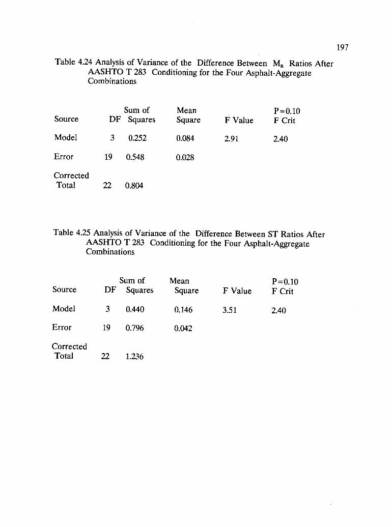
197
Table 4.24 Analysis of Variance of the Difference Between MR Ratios AfterAASHTO T 283 Conditioning for the Four Asphalt-AggregateCombinations
Sum of Mean P = 0.10Source DF Squares Square F Value F Crit
Model 3 0.252 0.084 2.91 2.40
Error 19 0.548 0.028
CorrectedTotal 22 0.804
Table 4.25 Analysis of Variance of the Difference Between ST Ratios AfterAASHTO T 283 Conditioning for the Four Asphalt-AggregateCombinations
Sum of Mean P=0.10Source DF Squares Square F Value F Crit
Model 3 0.440 0.146 3.51 2.40
Error 19 0.796 0.042
CorrectedTotal 22 1.236
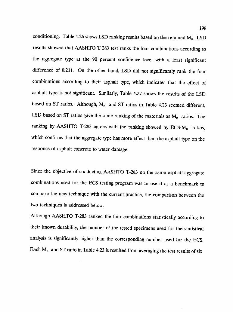
198
conditioning. Table 4.26 shows LSD ranking results based on the retained M. LSD
results showed that AASHTO T 283 test ranks the four combinations according to
the aggregate type at the 90 percent confidence level with a least significant
difference of 0.211. On the other hand, LSD did not significantly rank the four
combinations according to their asphalt type, which indicates that the effect of
asphalt type is not significant. Similarly, Table 4.27 shows the results of the LSD
based on ST ratios. Although, MR and ST ratios in Table 4.23 seemed different,
LSD based on ST ratios gave the same ranking of the materials as MR ratios. The
ranking by AASHTO T-283 agrees with the ranking showed by ECS-MR ratios,
which confirms that the aggregate type has more effect than the asphalt type on the
response of asphalt concrete to water damage.
Since the objective of conducting AASHTO T-283 on the same asphalt-aggregate
combinations used for the ECS testing program was to use it as a benchmark to
compare the new technique with the current practice, the comparison between the
two techniques is addressed below.
Although AASHTO T-283 ranked the four combinations statistically according to
their known durability, the number of the tested specimens used for the statistical
analysis is significantly higher than the corresponding number used for the ECS.
Each MR and ST ratio in Table 4.23 is resulted from averaging the test results of six
199
Table 4.26 Asphalt/Aggregate Ranking by MR
Alpha= 0.10 df= 19 MSE= 0.028889Least Significant Difference = 0.2119
Means with the same letter are not significantly different.
T Grouping Mean N Treatment
A 0.796 5 RB/AAK-1
B A 0.678 5 RB/AAG-1
B A 0.608 6 RL/AAK-1
B 0.510 7 RL/AAG-1
Table 4.27 Asphalt/Aggregate Ranking by LSD
Alpha= 0.10 df= 19 MSE= 0.041885Least Significant Difference = 0.2551
Means with the same letter are not significantly different.
T Grouping Mean N Treatment
A 0.852 5 RB/AAG-1
B A 0.712 5 RB/AAK-1
B A 0.622 6 RL/AAK-1
B 0.476 7 RL/AAG-1

200
specimens (three dry and three wet), so the total specimens used for this comparison
were 22X6 = 132 specimens. On the other hand, only 11 specimens (hot wet-
saturated conditioning) were used for the statistical analysis to rank the four
combinations according to ECS-MR ratios, as discussed earlier. The major difference
between the two techniques is that for AASHTO T-283 six specimens are needed in
order to get one MR ratio (or ST ratio). In contrast to AASHTO T-283, with ECS
technique three MR ratios are obtained by testing one specimen ( and the fourth one
after a freeze cycle).
For AASHTO T-283, the variation of MR and ST ratios with the same asphalt-
aggregate combination, which is expressed by high Coefficient of Variation compared
to those from the ECS procedure, and by present MR and ST ratios more than 1.0,
questions the repeatability of AASHTO T-283 and indicates that using this test as a
water sensitivity test needs more development.
The significant difference between AASHTO T-283 results in terms of the
repeatability confirms what has been discussed in proceeding sections about the role
of simulating the mechanisms of asphalt-aggregate interaction in the presence of
water in improving the repeatability of the test. Also, ECS test results show that
using one conditioning and testing device to perform all the tests on the same test
setup and one specimen orientation decreases the variability of the test results and
reduces the error sources associated with specimen handling and testing different
specimen orientations which is associated with AASHTO T-283.
201
Finally, from this comparison it has been concluded that AASHTO T 283, with its
current procedure, is a good moisture conditioning protocol to predict asphalt
concrete response to the change in mixture and conditioning variables of a water
conditioning protocol.
202
5. CONCLUSIONS
The following conclusions are based on the test results obtained in this laboratory
research and their analysis as presented. Conclusions that appear warranted are as
follows:
1. Comparisons between LVDTs and strain gages showed no significant
difference on dry specimens. However, the use of strain gages presented
problems regarding practicality during actual testing. That is, the strain gages
wrinkled under the effect of repeated loading with hot water conditioning.
Therefore, the use of LVDTs was adopted for strain measurement during the
resilient modulus tests.
2. Although the use of strain gages for the ECS was abandoned, tests on the
type of glue used to bond the gages to the specimens showed no significant
203
difference between glue types. The manufacturer recommended a super glue,
however.
3. The modulus tests on specimens having an L/D ratio of 5/4 showed
essentially the same very low variability and the same magnitude as those on
specimens with L/D ratios of 7/4. Backed by these results and the fact that
the 4-in. high by 4-in. diameter specimen is more representative of actual
pavement lift thicknesses, it was concluded that a specimen size of 4 in. diam.
by 4 in. high is more suitable than the conventional 4 in. by 2.5 in. high
specimen.
4. Tests investigating and evaluating the difference between the perforated and
solid teflon disks (employed to minimize shear stresses at the top and bottom
of the specimen during modulus testing) indicated that perforated disks are
suitable and that no significant difference exists between the two types. So, the
perforated disks are used rather than solid disks to provide openings for air
and water flow.
5. Regarding permeability measurement, it was shown that partially sealing the
specimen (sealing the middle third) with silicone cement is adequate; that is,
fully sealing the specimen is unnecessary - the two methods indicate no
significant difference.
6. Permeability is an appropriate measure of the void system in a mixture.
204
7. Retained MR, permeability (k), and stripping rate are suitable measures of
mixture behavior following various conditioning treatments such as degree of
wetting, temperature, and amount of air voids.
8. Three 6-hour temperature cycles are adequate to evaluate the effect of
conditioning. Longer (24-hour) cycles do not increase one's ability to discern
differences among mixtures.
9. Hot-wet cycling in the ECS is more detrimental than wet-freeze (without a hot
cycle) cycling and appears suitable for warm climates.
10. Tests investigating the effect of continuous repeated loading during hot-wet
cycling was (within the 200 lb. repeated load level) modest on Mr, while it
was significant on the stripping rate. That is, repeated loading has more
detrimental effect on adhesion.
11. Specimens with voids higher or lower than the pessimum range resist water
damage more than specimens within the pessimum range.
12. The comparison between the ECS and the current methods represented by
AASHTO T-283 showed that the ECS has better repeatability and needs
fewer specimens than AASHTO T-283 for performing a mix design.
13. The ECS as a test system is utilizing today's technology, which provides
continuous development in terms of test precision and convenient data
acquisition.
14. The ECS as a test method provides a number of parameters from the tested
specimen, i.e., retained MR, retained permeability, stripping rate, and more,
205
such as stress-strain information at different temperatures during the
conditioning procedure, which is available through the data acquisition
capability of the system. These data and capabilities will provide a better
understanding about asphalt-aggregate interaction and establish a reliable
base for a continuous education process.
15. Finally, regarding evaluation of the overall system, it was shown that the
system is sufficiently sensitive to detect the level of damage due to water in
terms of saturation level, conditioning temperature, and air voids level. In
short, the ECS has been demonstrated to be suitable for and capable of
determining the effect of water damage for a range of asphalt concrete
mixture.
206
6. RECOMMENDATIONS
6.1 Implementation
The overall goal of this research was to relate asphalt mixture properties to
performance of mixtures. The Environmental Conditioning System (ECS) was
developed and fabricated as a conditioning and testing device. The ECS was used
to explore the basic factors that influence the response of compacted mixtures to
water conditioning and was then used for modifying the water conditioning
procedure. Figure 6.1 shows the recommendations chart as accomplished in this
water sensitivity study. These recommendations are development of a testing
equipment and development of water conditioning techniques, which are discussed
in the following sections.
Testing Equipment
The ECS was devised and fabricated for water sensitivity testing and evaluation.
This device has been used for more than two years at different environmental
conditioning levels by including or excluding variability of related variables with
different treatment levels such as permeability, time of conditioning, rate of wetting,

207
Recommendations
Development and Fabricationof Testing System
Environmental Conditioning
System (ECS)
Water Conditioning Procedures
WET Conditioning Procedure
Water Conditioning Procedures
for Warm Climates for Cold Climates
Figure 6.1 Recommendation Chart as Accomplished in this Water Sensitivity Study
208
aging, loading, air voids, etc. The ECS shows a wide capability for environmental
conditioning and testing compacted asphalt mixtures. Although precision of tests has
not yet been developed, the ECS has a greater capability for simulating field
conditions to which the asphalt concrete is exposed better than previous methods.
Correspondingly, the ECS is a reliable testing device for water sensitivity and its
apparent advantages over previous methods are summarized in the following points:
1. The ECS monitors the permeability of the specimens after each
conditioning cycle, either thawing or freezing.
2. Eliminates leaking and specimen deformation during the test.
3. Decreases the variability of resilient modulus since only one specimen
setup is required.
4. Eliminates handling and transferring the specimen from water bath to
testing device, which is a possible major source of error.
5. The ECS allows the evaluation of the specimen after each phase of a
cycle, either freezing or thawing, instead of following a complete
conditioning cycle (freezing and thawing together).
6. The ECS conditions and tests compacted asphalt specimens with any
percent of air voids.
7. The ECS applies repeated loads throughout the duration of the test.
8. The ECS shows better repeatability than the current methods
represented by AASHTO T-283
209
9. The number of specimens needed for a mix design using the ECS
is less than the required specimens for the same purpose using
AASHTO T-283.
Water Conditioning Techniques
A series of tests were performed on four different MRL materials according to an
experiment plan which was established after selection to include the most important
related variables. Figure 6.2 shows the two recommended conditioning procedures.
These are summarized as follows:
Water Conditioning Procedure
In order to test the behavior of compacted asphalt mixtures, the ECS was used to
assist in determining the most important variables in the performance of mixtures in
the presence of moisture. An analysis was conducted on the test results to show
asphalt mixtures behavior in several ways:
Saturation vs. moisture
Wet vs. dry
Water vs. vapor
Water vs. air
Permeability vs. air void content
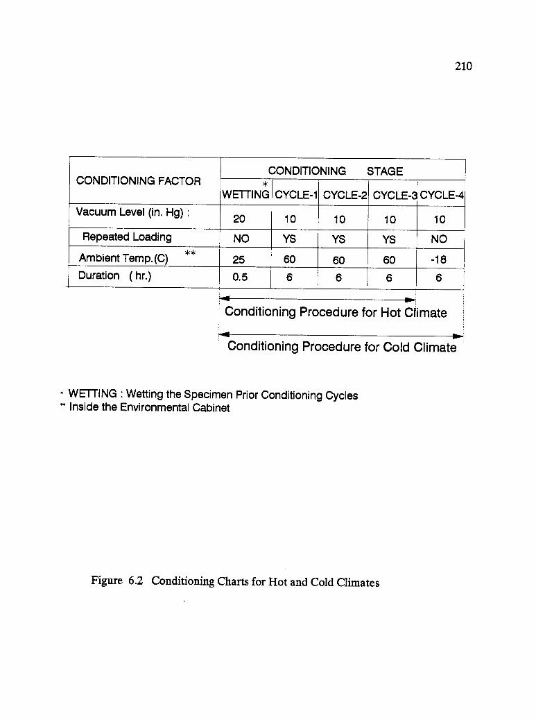
210
CONDITIONING FACTORCONDITIONING STAGE
*WETTING CYCLE-1 CYCLE-2 CYCLE-3 CYCLE-4
Vacuum Level (in. Hg) :20 10 10 10 10
Repeated Loading NO YS YS YS NO
Ambient Temp.(C) ** 25 60 60 60 -18
Duration ( hr.) 0.5 6 6 6 6
Conditioning Procedure for Hot Climate
Conditioning Procedure for Cold Climate
WETTING : Wetting the Specimen Prior Conditioning Cycles- Inside the Environmental Cabinet
Figure 6.2 Conditioning Charts for Hot and Cold Climates
211
Freeze vs. hot
Volume change effect
Conditioning time, such as cycle length
Dynamic loading vs. static loading
Stripping
The effect of each controlled variable in water sensitivity was measured by three
response variables which are:
Resilient modulus
Permeability
Stripping rate
From the analysis of the above variables, two water conditioning procedures were
recommended to give optimum simulation for asphalt mixture variables and give
practical acceleration for the highway agencies. The two water conditioning
procedures as shown in Figure 6.2 are as follows:
1. Water conditioning for warm climate: includes three wet-hot cycles of
6-hour duration at 60°C with continuous repeated loading.
2. Water conditioning for cold climate: includes three wet-hot cycles of
6-hour duration at 60°C with continuous repeated loading (as the hot
climate), plus one wet-freeze cycle of the same duration as the hot
cycle with static loading at - 18°C.
212
Repeated loading is performed during the hot cycles for the two procedures.
Figure 6.2 shows the conditioning charts for the two procedures, and the details are
shown in Appendices B and C.
Wet Conditioning Procedure
Wet conditioning is identified by the term "Wetting" in Figure 6.2. Wet conditioning
is a wetting process by running water (under vacuum) through compacted asphalt
concrete specimens at ambient 25°C temperature for 30 minutes. Wet conditioning
is recommended to be performed prior to testing in fatigue, rutting, and low
temperature cracking. The wet conditioning procedure, including specimen setup
recommendations for cylindrical and beam specimens, is shown in Appendix C.
213
6.2 Future Research
Additional research of moisture damage in asphalt concrete is recommended. The
following suggested research is not covered by any known previous study or by this
study:
1. Although the visual evaluation rating standard developed in this study has
been found practical, it still includes human subjectivity in deciding the rate
of stripping. Since the stripping rate is a very good evaluation method for
water damage, because it is related to the adhesion bond, there is a need for
developing an objective stripping rate standard test. Using an electronic
scanner technique could be the key for the required development. Although
a scanner includes the broken aggregate as a stripped aggregate, this problem
can be controlled by coloring the broken aggregates with a black color, or by
scanning a similar unconditioned specimen, then subtracting the result of the
stripping rate of the unconditioned specimen from the stripping rate of the
conditioned one.
2. The application of the recommended wetting procedure in this study needs to
be applied to wet asphalt concrete specimens to determine the effect of the
wetting on fatigue life, low temperature cracking, and the aging process.
214
7. REFERENCES
Al-Ohaly, A.A. and Terrel, R. L.(1989). "Effects of microwave heating onadhesion and moisture damage of asphalt mixtures, " TRR 1171,Transportation Research Board.
AASHTO, "Resistance of Computed Bituminous Mixtures to MoistureInduced Damage," AASHTO T283-85.
AASHTO, "Effect of Water on Cohesion of Compacted BituminousMixtures," AASHTO T165-82.
AASHTO, "Coating and Stripping of Bituminous-Aggregate Mixtures,"AASHTO T182-82.
AASHTO, "Resistance to Plastic Flow of Bituminous Mixtures Using MarshallApparatus," AASHTO 1245-82.
Al-Swailmi, S., and Terrel, R.L. (1992). " Evaluation of Water Damage ofAsphalt Concrete Mixtures Using the Environmental ConditioningSystem (ECS)," Journal of the Association of Asphalt PavingTechnologists, Charleston, South Carolina, 1992.
Al-Swailmi, S., Scholz, T.V., and Terrel, R.L. (1992). " The Development andEvaluation of a Test System to Induce and Monitor Moisture Damageto Asphalt Concrete Mixtures," Transportation Research BoardMeeting, Washington, DC.
ASTM, "Test for Effect of Water on Bituminous Coated Aggregate," ASTMD 3625-77.
ASTM, "Effect of Water on Cohesion of Compacted Bituminous Mixtures,"ASTM D 1075-81.
ASTM, "Coating and Stripping of Bituminous-Aggregate Mixtures," ASTMD1664-80.
215
ASTM, "The Standard Test Method for Dynamic Modulus of AsphaltMixtures," ASTM D3497.
ASTM, "The Standard Method of Indirect Tension Test for Resilient Modulusof Bituminous Mixtures," ASTM D4123.
ASTM, "The Standard Capping Method," ASTM C617.
ASTM, "Bulk Specific Gravity of Compacted Bituminous Mixtures UsingParaffin-Coated Specimens," ASTM D1188.
ASTM, "Bulk Specific Gravity of Compacted Bituminous Mixtures UsingSaturated Surface-Dry Specimen," ASTM D2726.
ASTM, "Standard Terminology for Statistical Methods," ASTM E 456.
ASTM, "Standard Practice for Conducting an Inter Laboratory Test Programto Determine the Precision of Test Methods for ConstructionMaterials," ASTM C 802.
ASTM, "Standard Practice for Use of the Terms Precision and Bias in ASTMTest Methods," ASTM E 177.
Blight, G.E. (1977),"A falling head air permeameter for testing asphalt," DieSivielle Ingenieur in Suid-Afrika.
Curtis, W.C., Ens ley, K., and Epps, J., Draft Final Report on FundamentalProperties of Asphalt-Aggregate Interactions Including Adhesion andAbsorption, Strategic Highway Research Program, National ResearchCouncil, Washington, DC, 1992.
Curtis, C., Terrel, R.L., Perry, L.M., Al-Swailmi, S., and Brannon, E.J.,"Asphalt-Aggregate Interactions," Journal Association of AsphaltPaving Technologists, 1991.
Del Valle, H. (1985). "Procedure-Bulk specific gravity of compactedbituminous mixtures using parafilm-coated specimens," ChevronResearch Company, Richmond, California.
Ellis, W.H. and Schmidt, R. J.,(1960) "A Method for measuring the airpermeability of asphalt concrete pavements," ASTM Special TechnichalPublication No. 294.
216
Eriksen, K., (1991), Quarterly Report on Microscopical Analysis of Asphalt-Aggregate Mixtures Related to Pavement Performance, StrategicHighway Research Program, National Research Council, Washington,DC, September, 1991.
Field, F. and Phang, W.A. (1986). "Stripping in asphaltic concrete mixes:observations and test procedures," Proceedings, 12th AnnualConference of the Canadian Technical Asphalt Association, Halifax.
Goode, J.F. and Lutsey, L.A. (1965). "Voids, Permeability, Film Thicknessvs. Asphalt Hardening", Proceedings, Association of Asphalt PavingTechnologists, 34, 430-462.
Graf, P.E. (1986). Discussion of "Factors affecting moisture susceptibility ofasphalt concrete mixes", Proceedings, Association of Asphalt PavingTechnologists, 55, 175-212.
Hein, T.C. and Schmidt, R.J. (1961). "Air Permeability ofAsphalt Concrete",American Society for Testing and Materials, ASTM Special TechnichalPublication No. 309.
Kennedy, T.W., Roberts, F.L., and Lee, K.W., (1982) "Evaluation of MoistureSusceptibility of Asphalt Mixtures Using the Texas Freeze-ThawPedestal Test," Proceedings, Assoc. Asphalt Paving Technol., 51.
Kennedy, T.W., Roberts, F.L., Lee, K.W. (1983). "Evaluation of moistureeffects on asphalt concrete mixtures," TRR 911, TransportationResearch Board. Washington, DC.
Kumar, A. and Goetz, W.H. (1977). "Asphalt hardening as affected by filmthickness, voids, and permeability in asphaltic mixtures," Proceedings,Association of Asphalt Paving Technologists, San Antonio.
Kumar, A. and Goetz, W.H. (1977). "Laboratory measurement ofpermeability of compacted asphalt mixtures," TRR 659, TransportationResearch Board. Washington, DC.
Lottman, R.P. (1971). "The moisture mechanism that causes asphalt strippingin asphaltic pavement mixtures," Department of Civil Engineering,University of Idaho, Final Report.
217
Lottman, R.P. (1978). "Predicting moisture-induced damage to asphalticconcrete," NCHRP 192, Transportation Research Board. Washington,DC.
Lottman, R.P. (1982). "Prediction moisture-induced damage to asphalticconcrete - field evaluation," NCHRP 246, Transportation ResearchBoard.
Majidzadeh, K. and Brovold, F.N. (1968). "State of the art: effect of wateron bitumen-aggregate mixtures," Highway Research Board, SpecialReport 98.
Mandel, J.,(1964),"The Statistical Analysis of Experiment Data," John Wiley& Sons, New York.
Parker, F. and Gharaybeh, F. (1987). "Evaluation of indirect tensile tests forassessing stripping of Alabama asphalt concrete mixtures," TRR 1115,Transportation Research Board, 113-124. Washington, DC.
Parker, F., and Wilson, M.S. (1986). "Evaluation of boiling and stresspedestal tests for assessing stripping potential of Alabama asphaltconcrete mixtures," TRR 1096, Transportation Research Board, 90-99.
Podoll, R. T., (1991), Monthly Progress Report on Surface Analysis By LaserIonization of the Asphalt-Aggregate Bond, Strategic Highway ResearchProgram, National Research Council, Washington, DC., June, 1991.
Rensel, Paul (1965). "Simplified quality control of asphalt concrete",Proceedings, Northwest Roads and Streets Conference, University ofWashington, Seattle.
Schmidt, R.J. and Graf, P.D. (1972). "The effect of water on the resilientmodulus of asphalt treated mixes," Proceedings, Association of AsphaltPaving Technologists, 41, 118-162.
Shute, J.W., R.G. Hicks, J.E. Wilson, and L.G. Scholl (1989). "Effectivenessof antistripping additives," Vols. I and II, Oregon DOT, May 1989.
Stuart, K.D. (1986). "Evaluation of procedures used to predict moisturedamage in asphalt mixtures," FHWA/RD-86/091.
Terrel, R.L. and J.W. Shute (1989). "Summary report on water sensitivity,"SHRP-A/IR-89-003, Strategic Highway Research Program.
218
Terrel, R.L. (1990). "Water sensitivity of asphalt concrete," Proceedings,New Mexico Paving and Transportation Conference.
Tunnicliff, D.G., and Root, R.E. (1984). "Use of antistripping additives inasphaltic concrete mixtures," NCHRP 274, Transportation ResearchBoard.
Vallerga, B.A. and Hicks, R.G. (1968). "Water permeability of asphaltconcrete specimens using back-pressure saturation," Journal ofMaterials, 3(1). Washington, DC.

8. APPENDICES
219
APPENDIX A
ORIGINAL TEST RESULTS OF ECS
In order to make it convenient for conducting different studies which may not beincluded in this research, this appendix includes the whole ECS conditioning data.Two groups of data are included in Appendix A:
1- Table A-1: the original data of the ECS tests results from 4 in.-high specimens,which are included in section 3 (Table 3.8) after averaging the replicates,
2- Table A-2 : the original data of the ECS results from 2.5 inch-high specimenswhich are not discussed in this report because of the high variability associated withMR, but still could be used for further analysis for the variability of the MR test orsome other studies related to the other reported data (i.e., air voids, permeabilityetc.).
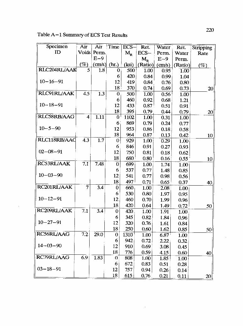
220Table A-1 Summary of ECS Test Results
SpecimenID
AirVoids
(%)
AirPerm.E-9(cm/s)
Time
(hr.)
ECS-MR
(ksi)
Ret.ECS-
MR(Ratio)
WaterPerm.E -9(cm/s)
Ret.WaterPerm.(Ratio)
StrippingRate
(%)RLC204RL/AAK 5 1.8 0 500 1.00 0.95 1.00
6 420 0.84 0.99 1.0410-16-91 12 419 0.84 0.76 0.80
18 370 0.74 0.69 0.73 20RLC91RL/AAK 4.5 1.3 0 500 1.00 0.56 1.00
6 460 0.92 0.68 1.2110-18-91 12 433 0.87 0.51 0.91
18 395 0.79 0.44 0.79 20RLC58RB/AAG 4 1.11 0 1102 1.00 0.31 1.00
6 869 0.79 0.24 0.7710- 5 90 12 953 0.86 0.18 0.58
18 964 0.87 0.13 0.42 10RLC118RB/AAC 4.3 1.7 0 929 1.00 0.29 1.00
6 846 0.91 0.27 0.9302-08-91 12 750 0.81 0.18 0.62
18 680 0.80 0.16 0.55 10RC53RL/AAK 7.1 7.48 0 699 1.00 1.74 1.00
6 537 0.77 1.48 0.8510-03-90 12 541 0.77 0.98 0.56
18 497 0.71 0.65 0.37 40RC201RL/AAK 7 3.4 0 660 1.00 2.08 1.00
6 530 0.80 1.97 0.9510-12-91 12 460 0.70 1.99 0.96
18 420 0.64 1.49 0.72 50RC209RL/AAK 7.1 3.4 0 420 1.00 1.91 1.00
6 345 0.82 1.84 0.9610 -27 -91 12 320 0.76 1.61 0.84
18 250 0.60 1.62 0.85 50RC56RI/AAG 7.2 29.0 0 1310 1.00 6.87 1.00
6 942 0.72 2.22 0.3214-03-90 12 910 0.69 3.08 0.45
18 776 0.59 4.15 0.60RC79RL/AAG 6.9 1.83 0 808 1.00 1.85 1.00
6 672 0.83 0.51 0.2803-18-91 12 757 0.94 0.26 0.14
18 615 0.76 0.21 0.11 20
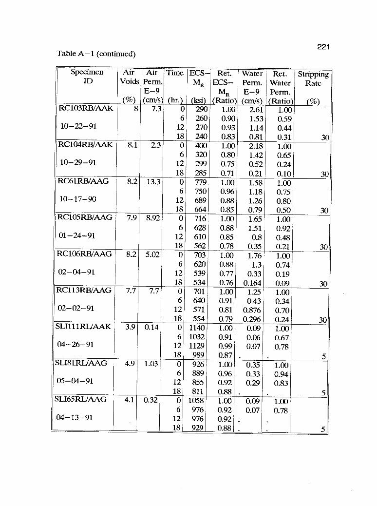
221Table A-1 (continued)
SpecimenID
AirVoids
(%)
AirPerm.E -9(cm/s)
Time
(hr.)
ECS-MR
(Icsi)
Ret.ECS-
MR(Ratio)
WaterPenn.E-9(cm/s)
Ret.WaterPenn.(Ratio)
StrippingRate
(%)RC103RB/AAK 8 7.3 0 290 1.00 2.61 1.00
6 260 0.90 1.53 0.5910-22-91 12 270 0.93 1.14 0.44
18 240 0.83 0.81 0.31 30RC104RB/AAK 8.1 2.3 0 400 1.00 2.18 1.00
6 320 0.80 1.42 0.6510-29-91 12 299 0.75 0.52 0.24
18 285 0.71 0.21 0.10 30RC61RB/AAG 8.2 13.3 0 779 1.00 1.58 1.00
6 750 0.96 1.18 0.7510-17-90 12 689 0.88 1.26 0.80
18 664 0.85 0.79 0.50 30RC105RB/AAG 7.9 8.92 0 716 1.00 1.65 1.00
6 628 0.88 1.51 0.9201-24-91 12 610 0.85 0.8 0.48
18 562 0.78 0.35 0.21 30RC106RB/AAG 8.2 5.02 0 703 1.00 1.76 1.00
6 620 0.88 1.3 0.7402-04-91 12 539 0.77 0.33 0.19
18 534 0.76 0.164 0.09 30RC113RB/AAG 7.7 7.7 0 701 1.00 1.25 1.00
6 640 0.91 0.43 0.3402-02-91 12 571 0.81 0.876 0.70
18 554 0.79 0.296 0.24 30SLI111RUAAK 3.9 0.14 0 1140 1.00 0.09 1.00
6 1032 0.91 0.06 0.6704-26-91 12 1129 0.99 0.07 0.78
18 989 0.87 . 5SLI81RLJAAG 4.9 1.03 0 926 1.00 0.35 1.00
6 889 0.96 0.33 0.9405-04-91 12 855 0.92 0.29 0.83
18 811 0.88 . 5SLI65RL/AAG 4.1 0.32 0 1058 1.00 0.09 1.00
6 976 0.92 0.07 0.7804-13-91 12 976 0.92 .
18 929 0.88 . .
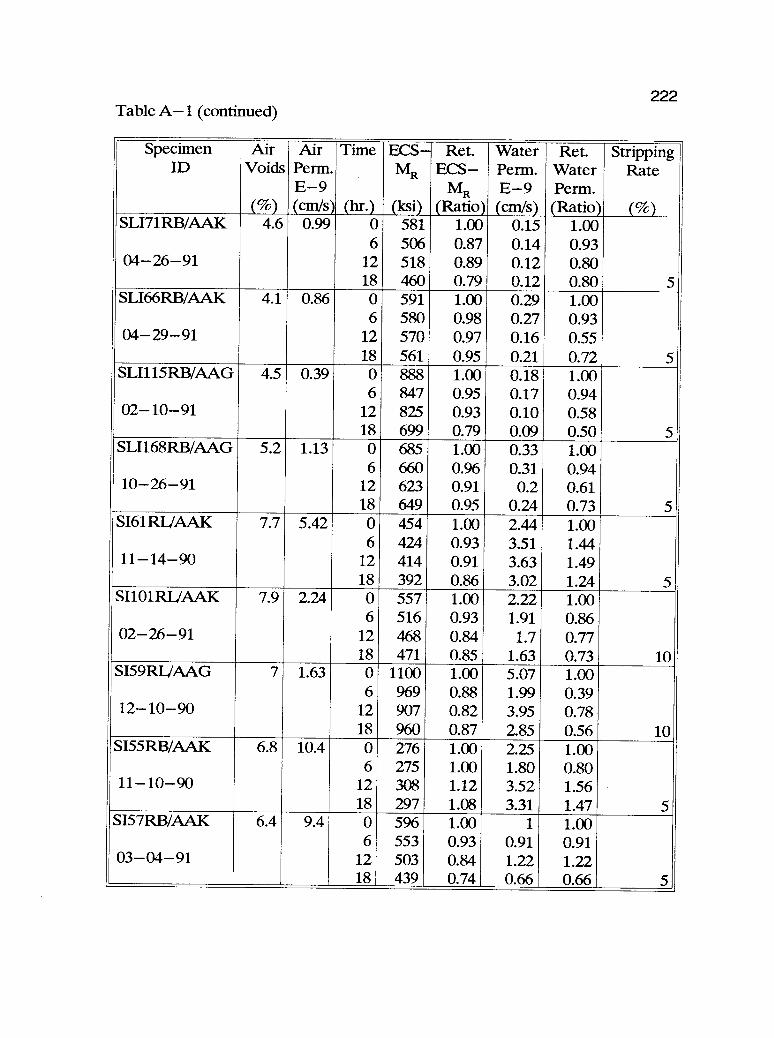
222Table A-1 (continued)
SpecimenID
AirVoids
(%)
AirPerm.E-9(cm/s)
Time
(hr.)
ECS-MR
(Icsi)
Ret.ECS-
MR(Ratio)
WaterPerm.E-9(cm/s)
Ret.WaterPerm.(Ratio)
StrippingRate
(%)SLI71RB/AAK 4.6 0.99 0 581 1.00 0.15 1.00
6 506 0.87 0.14 0.9304-26-91 12 518 0.89 0.12 0.80
18 460 0.79 0.12 0.80 5SLI66RB/AAK 4.1 0.86 0 591 1.00 0.29 1.00
6 580 0.98 0.27 0.9304-29-91 12 570 0.97 0.16 0.55
18 561 0.95 0.21 0.72 5SLI115RB/AAG 4.5 0.39 0 888 1.00 0.18 1.00
6 847 0.95 0.17 0.9402 -10 -91 12 825 0.93 0.10 0.58
18 699 0.79 0.09 0.50 5SLI168RB/AAG 5.2 1.13 0 685 1.00 0.33 1.00
6 660 0.96 0.31 0.9410 -26 -91 12 623 0.91 0.2 0.61
18 649 0.95 0.24 0.73 5SI61RL/AAK 7.7 5.42 0 454 1.00 2.44 1.00
6 424 0.93 3.51 1.4411-14-90 12 414 0.91 3.63 1.49
18 392 0.86 3.02 1.24 5SI101RL/AAK 7.9 2.24 0 557 1.00 2.22 1.00
6 516 0.93 1.91 0.8602-26-91 12 468 0.84 1.7 0.77
18 471 0.85 1.63 0.73 10S159R1JAAG 7 1.63 0 1100 1.00 5.07 1.00
6 969 0.88 1.99 0.3912 -10 -90 12 907 0.82 3.95 0.78
18 960 0.87 2.85 0.56 10SI55RB/AAK 6.8 10.4 0 276 1.00 2.25 1.00
6 275 1.00 1.80 0.8011 -10 -90 12 308 1.12 3.52 1.56
18 297 1.08 3.31 1.47 5SI57RB/AAK 6.4 9.4 0 596 1.00 1 1.00
6 553 0.93 0.91 0.9103-04-91 12 503 0.84 1.22 1.22
18 439 0.74 0.66 0.66 5
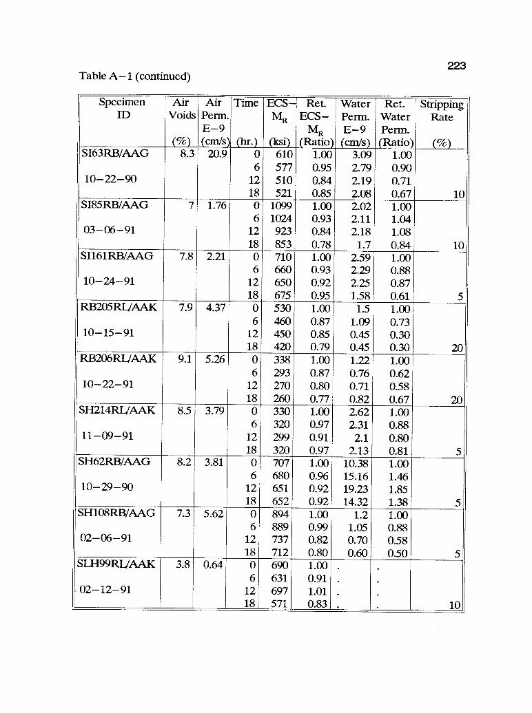
223Table A-1 (continued)
SpecimenID
AirVoids
(%)
AirPerm.E -9(culls)
Time
(hr.)
ECS-MR
(Icsi)
Ret.ECS-
MR(Ratio)
WaterPenn.E -9(cm/s)
Ret.WaterPerm.(Ratio)
StrippingRate
(%)SI63RB/AAG 8.3 20.9 0 610 1.00 3.09 1.00
6 577 0.95 2.79 0.9010 -22 -90 12 510 0.84 2.19 0.71
18 521 0.85 2.08 0.67 10SI85RB/AAG 7 1.76 0 1099 1.00 2.02 1.00
6 1024 0.93 2.11 1.0403 -06 -91 12 923 0.84 2.18 1.08
18 853 0.78 1.7 0.84 10SI161RB/AAG 7.8 2.21 0 710 1.00 2.59 1.00
6 660 0.93 2.29 0.8810-24-91 12 650 0.92 2.25 0.87
18 675 0.95 1.58 0.61 5RB205RIJAAK 7.9 4.37 0 530 1.00 1.5 1.00
6 460 0.87 1.09 0.7310-15-91 12 450 0.85 0.45 0.30
18 420 0.79 0.45 0.30 20RB206RL/AAK 9.1 5.26 0 338 1.00 1.22 1.00
6 293 0.87 0.76 0.6210 -22 -91 12 270 0.80 0.71 0.58
18 260 0.77 0.82 0.67 20SH214RL/AAK 8.5 3.79 0 330 1.00 2.62 1.00
6 320 0.97 2.31 0.8811-09-91 12 299 0.91 2.1 0.80
18 320 0.97 2.13 0.81 5SH62RB/AAG 8.2 3.81 0 707 1.00 10.38 1.00
6 680 0.96 15.16 1.4610 -29 -90 12 651 0.92 19.23 1.85
18 652 0.92 14.32 1.38 5SH108RWAAG 7.3 5.62 0 894 1.00 1.2 1.00
6 889 0.99 1.05 0.8802-06 91 12 737 0.82 0.70 0.58
18 712 0.80 0.60 0.50 5SLH99RUAAK 3.8 0.64 0 690 1.00 .
6 631 0.91 .
02-12-91 12 697 1.01 . .
18 571 0.83 . 10
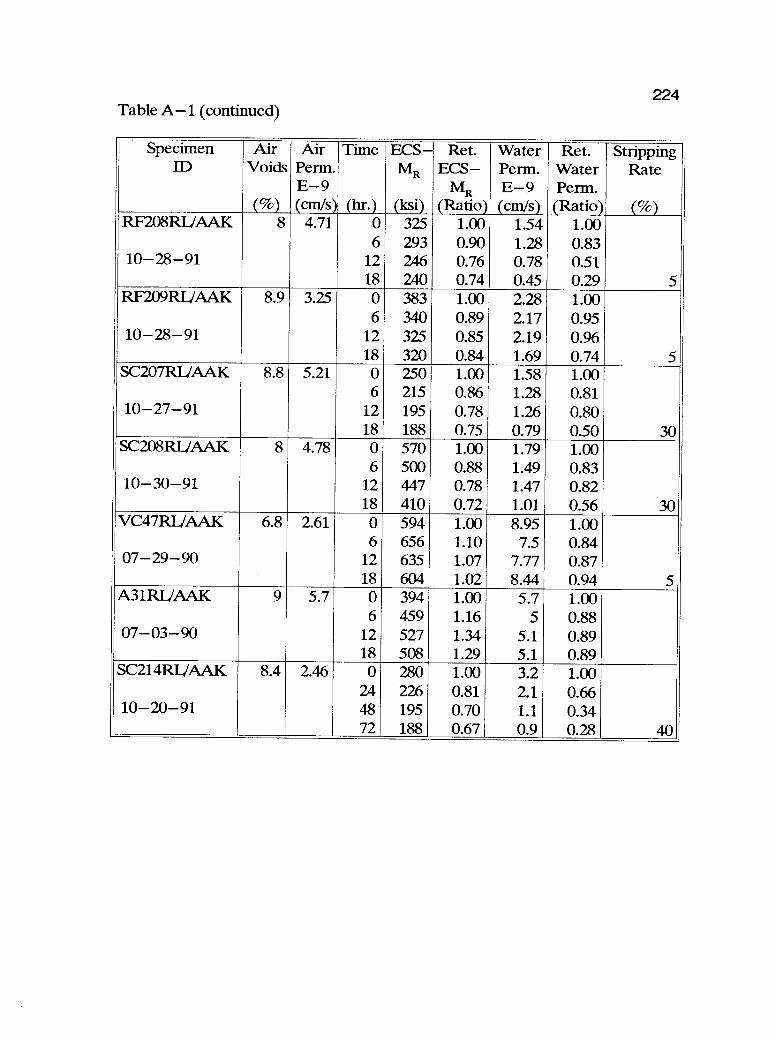
224Table A-1 (continued)
SpecimenID
AirVoids
(%)
AirPerm.E -9(cm/s)
Time
(hr.)
ECS-MR
(ksi)
Ret.ECS-
MR(Ratio)
WaterPerm.E-9(cm/s)
Ret.WaterPenn.
(Ratio)
StrippingRate
(%)RF208RIJAAK 8 4.71 0 325 1.00 1.54 1.00
6 293 0.90 1.28 0.8310 -28 -91 12 246 0.76 0.78 0.51
18 240 0.74 0.45 0.29 5RF209RIJAAK 8.9 3.25 0 383 1.00 2.28 1.00
6 340 0.89 2.17 0.9510- 28- 91 12 325 0.85 2.19 0.96
18 320 0.84 1.69 0.74 5SC207RL/AAK 8.8 5.21 0 250 1.00 1.58 1.00
6 215 0.86 1.28 0.8110 -27 -91 12 195 0.78 1.26 0.80
18 188 0.75 0.79 0.50 30SC208RL/AAK 8 4.78 0 570 1.00 1.79 1.00
6 500 0.88 1.49 0.8310 -30 -91 12 447 0.78 1.47 0.82
18 410 0.72 1.01 0.56 30VC47RL/AAK 6.8 2.61 0 594 1.00 8.95 1.00
6 656 1.10 7.5 0.8407-29-90 12 635 1.07 7.77 0.87
18 604 1.02 8.44 0.94 5A31RIJAAK 9 5.7 0 394 1.00 5.7 1.00
6 459 1.16 5 0.8807 -03 -90 12 527 1.34 5.1 0.89
18 508 1.29 5.1 0.89SC214RL/AAK 8.4 2.46 0 280 1.00 3.2 1.00
24 226 0.81 2.1 0.6610-20-91 48 195 0.70 1.1 0.34
72 188 0.67 0.9 0.28 40
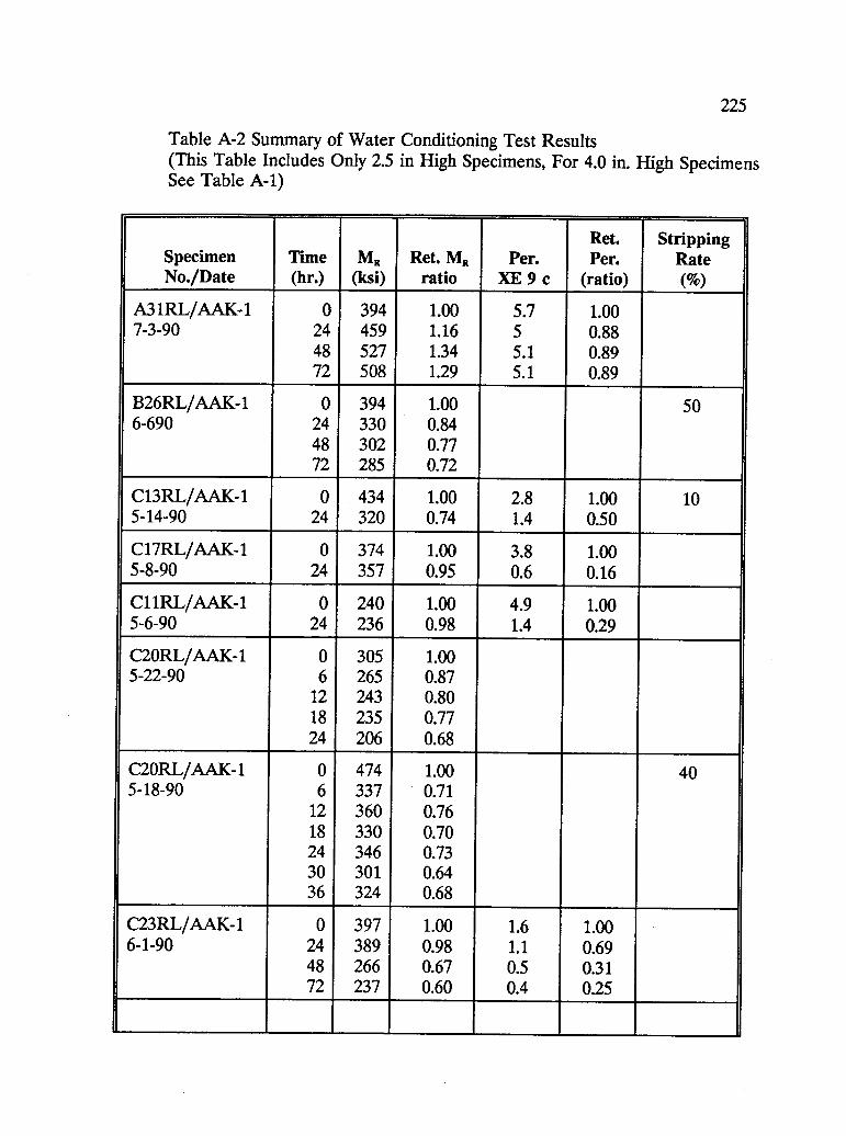
225
Table A-2 Summary of Water Conditioning Test Results(This Table Includes Only 2.5 in High Specimens, For 4.0 in. High SpecimensSee Table A-1)
SpecimenNo./Date
Time(hr.)
M.(ksi)
Ret. M.ratio
Per.ME 9 c
Ret.Per.
(ratio)
StrippingRate(%)
A31RL/AAK-1 0 394 1.00 5.7 1.007-3-90 24 459 1.16 5 0.88
48 527 1.34 5.1 0.8972 508 1.29 5.1 0.89
B26RL/AAK-1 0 394 1.00 506-690 24 330 0.84
48 302 0.7772 285 0.72
Cl3RL/AAK-1 0 434 1.00 2.8 1.00 105-14-90 24 320 0.74 1.4 0.50
CIIRL/AAK-1 0 374 1.00 3.8 1.005-8-90 24 357 0.95 0.6 0.16
Cl1RL/AAK-1 0 240 1.00 4.9 1.005-6-90 24 236 0.98 1.4 0.29
C2ORL/AAK-1 0 305 1.005-22-90 6 265 0.87
12 243 0.8018 235 0.7724 206 0.68
C2ORL/AAK-1 0 474 1.00 405-18-90 6 337 0.71
12 360 0.7618 330 0.7024 346 0.7330 301 0.6436 324 0.68
C23RL/AAK-1 0 397 1.00 1.6 1.006-1-90 24 389 0.98 1.1 0.69
48 266 0.67 0.5 0.3172 237 0.60 0.4 0.25

Table A-2 (continued)
226
SpecimenNo./Date
Time(hr.)
MR(ksi)
Ret. MRratio
Per.XE 9 c
Ret.Per.
(ratio)
StrippingRate(%)
F25RL/AAK-1 0 297 1.00 4.7 1.00 106-3-90 24 247 0.83 3.1 0.66
48 279 0.94 3.1 0.6672 200 0.67 33 0.70
F29RL/AAK-1 0 394 1.00 3.4 1.006-19-90 24 260 0.66 1 029
38 270 0.69 0.9 0.2672 300 0.76 0.4 0.12
H28RL/AAK-1 0 340 1.00 23 1.00 206-15-90 24 329 0.97 0 0.00
48 244 0.72 0 0.0072 245 0.72 0 0.00
127RL/AAK-1 0 218 1.00 3.10 1.00 106-10-90 24 248 1.14 0 0.00
48 218 1.00 0 0.0072 242 1.11 0.00
132RL/AAK-1 0 312 1.00 2.4 1.007-7-90 24 215 0.69 2.7 1.13
48 228 0.723 7.8 3.2572 210 0.67 9.7 4.04
L12RL/AAK-1 0 331 1.00 6.1 1.005-17-90 24 191 0.58 0.9 0.15
AG 19RL/AAK- 0 266 1.00 5 1.00 0.01 3 332 1.25 5.4 1.085-25-90 6 354 133 5.4 1.08
9 350 132 5.6 1.1212 365 137 5.4 1.0818 401 1.51 5.6 1.12
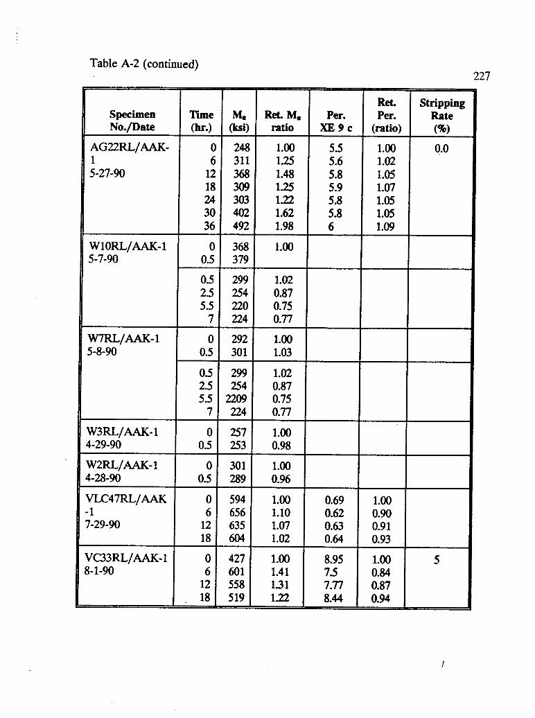
Table A-2 (continued)227
SpecimenNo./Date
Time(hr.)
M.(ksi)
Ret. M.ratio
Per.XE 9 c
Rd.Per.
(ratio)
StrippingRate(%)
AG22RL/AAK- 0 248 1.00 5.5 1.00 0.01 6 311 1.25 5.6 1.025-27-90 12 368 1.48 5.8 1.05
18 309 1.25 5.9 1.0724 303 1.22 5.8 1.0530 402 1.62 5.8 1.0536 492 1.98 6 1.09
W1ORL/AAK- 1 0 368 1.005-7-90 0.5 379
0.5 299 1.022.5 254 0.875.5 220 0.75
7 224 0.77
W7RL/AAK-1 0 292 1.005-8-90 0.5 301 1.03
0.5 299 1.022.5 254 0.875.5 2209 0.75
7 224 0.77
W3RL/AAK-1 0 257 1.004-29-90 05 253 0.98
W2RL/AAK-1 0 301 1.004-28-90 0.5 289 0.96
VLC47RL/AAK 0 594 1.00 0.69 1.00-1 6 656 1.10 0.62 0.907-29-90 12 635 1.07 0.63 0.91
18 604 1.02 0.64 0.93
VC33RL/AAK-1 0 427 1.00 8.95 1.00 58-1-90 6 601 1.41 7.5 0.84
12 558 131 7.77 0.8718 519 1.22 8.44 0.94
228
APPENDIX B
STANDARD METHOD OF TEST FORDETERMINING MOISTURE SENSITIVITY CHARACTERISTICSOF COMPACTED BITUMINOUS MIXTURES SUBJECTEDTO HOT AND COLD CLIMATE CONDITIONS
The test method is in a format similar to the test methods contained in the American Associationof State Highway and Transportation Officials' (AASHTO) standard specifications. At the conclusionof SHRP, selected test methods will be submitted to AASHTO for adoption into its standardspecifications.
1. SCOPE
1.1 This method describes conditioning procedures intended to determine the moisturesensitivity or stripping characteristics of a compacted bituminous mixture in the laboratory under hotand cold climatic conditions. Environmental variables such as temperature, moisture and load are usedin the procedure.
2. APPLICABLE DOCUMENTS
21 AASHTO Test Methods:T247-80 Preparation of Test Specimens of Bituminous Mixtures by Means ofCalifornia Kneading Compactor
T167-84 Compressive strength of Bituminous Mixtures
22 ASTM Test Methods:D 1561-81a Preparation of Bituminous Mixture Test Specimens by Means ofCalifornia Kneading Compactor
D 3497-79 Standard Test Method for Dynamic Modulus of Asphalt Mixtures
D 3549-83 Thickness or Height of Compacted Bituminous Paving Mixture Specimens
D 4013-81 Standard Practice for Preparation of Test Specimens of BituminousMixtures by Means of Gyratory Shear Compactor
3. APPARATUS 229
3.1 Test System - A Environmental Conditioning System (ECS) capable of simulating ahot or cold climatic regime to condition a compacted bituminous mixture specimen. Periodicmeasurements of the modulus (defined as the ECS modulus or ECS-MR) of the specimen will bemade throughout the test. In addition, air permeability of the specimen is measured before theconditioning begins.
The ECS-MR is similar to the dynamic modulus defined in ASTM D3497-79. However, thereare 2 important differences; 1) the height of the specimen is 4 in. instead of 8 in., and 2) thespecimen is encapsulated in a rubber membrane throughout the test.
Figures 1 and 2 present diagrams of a test system which is capable of performing the requiredtesting. Figure 1 is an illustration of the test setup with a specimen ready for testing and Figure 2 isa schematic drawing of the ECS setup. After the specimen has been prepared, it is placed in the ECSand the initial (dry) ECS-MR and air permeability determined. The specimen then undergoes awetting procedure at 25°C where a vacuum equivalent to 20 in. of mercury (Hg) is used to pulldistilled water through the specimen for 30 minutes. At the end of 30 minutes (wetting stage), thewater permeability is measured.
Before the conditioning begins, the vacuum is reduced from 20 in. to 10 in. of Hg, and thewater flow is adjusted to a maximum flow of 5 cc/min. This is to maintain water replacement for theair bubbles coming out from the specimen during the hot conditioning cycles as well as the coolingand thawing periods. For the hot conditioning cycle, the temperature of the environmental cabinet(ambient temperature) is set to 60°C. After 6 hours, the temperature is changed back to the testingtemperature of 25°C ± 0.5°C. After 2 additional hours (i.e. a total of 8 hours), the ECS-MR andwater permeability are measured. Throughout the hot conditioning cycle, a repeated load (haversine,0.1s on, 0.9s off, with a magnitude of 30 lbs static and 200 lbs dynamic load) is applied.
For hot climate conditioning, the hot 6-hour cycle is repeated for a total of 3 cycles (total of24 hours) for each specimen. If the bituminous mixture is to be used in a cold climate, the three hot6-hour cycles are followed by one cold 6-hour cycle. The cold cycle is similar to the hot cycle;however, the temperature is changed to -18°C (instead of60°C), and no repeated loading is applied.Distilled water continues to be pulled through the specimen at a vacuum of 10 in. of Hg . After 6hours at -18°C, the temperature is brought to 25°C for 2 hours, and the ECS-MR and waterpermeability is measured again at the end of the conditioning cycle. The ECS-MR and waterpermeability measurements are made at the end of each 6-hour conditioning cycle. Figure 3 illustratesthe conditioning procedures for both hot and cold climates.
As a minimum, the test system should meet the following requirements:
J-oad Measurement
Range: 0 to 1000 lbf tensionResolution: s 0.5 IbtAccuracy: ± 1% Full Scale
Deformation
Range: 0 to 0.25 inchResolution: I 5 x 10⁴ inchAccuracy: ± 5 x 104 inch
Temperature
Range: -20°C to 100°CResolution: I 0.5°CAccuracy: I 0.5°C
Vacuum
Range: 0 to 25 in. HgResolution: I 1.0 in. HgAccuracy: t 0.5 in. Hg
Air Flow
Range: 20 cc/min to 40 scfhResolution: s 20 cc/minAccuracy: t 10 cc/min
Water Flow
230
Range: 0 to 40 gphResolution: s 1 cc/minAccuracy: t 0.5 cc/min
3.2 Testing Machine - A mechanical or hydraulic testing machine that meets therequirements of AASHTO T167-84.
33 Specimen Holder - A specimen holder capable of holding a 4 in. diameter by 4 in. highbituminous specimen is required for the sealing process. See Figure 4.
3.4 End Platens - Two 4 in. diameter by 2 in. thick aluminum platens. One side of theplatens will have a drainage hole as well as a pattern of grooves as shown in Figure 5. Platens shallalso have a ane4ixteenth (1/16th) in. diameter 0-ring groove.
3.5 Afocellaneous Apparatus:
Metal tape or ruler/set of calipersSource of compressed air1.5 and 6 in. lengths of rubber membrane (4 in. diameter)2 Linear Variable Differential Transformers (LVDTs)Clear silicone cementVacuum source
10 gallons of distilled water
4. TEST SPECIMENS
231
4.1 Compacted Bituminous Concrete Specimens - Specimens shall be cored from a slabprepared with the use of a rolling wheel compactor or as molded if prepared by kneading or gyratorycompaction. It is rLot recommended that the Marshall method of compaction be used (AASHTOT245-82 or ASTI( D 1559-89). If specimens are cored, the top and bottom of the specimen shall tabe cut. Specimens shall be 4.0 t 0.15 inches high and 4.0 t 0.15 inches in diameter.
4.2 Measurement of Specimen Size - Measure the specimen at four locations, atapproximately quarter points and record the average measurement as the thickness of the specimenwithin t 0.15 cm. Measure the diameter of the specimen in the same fashion. Determine thespecimen cross sectional area as described in Section 6.1.
4.3 Sealing the Specimen - Place the specimen on the specimen holder and apply siliconecement in the middle of the specimen wall. Apply a large enough bead such that a surface 1.5 incheswide is uniformly covered. Place a cylindrical rubber membrane 1.5 inches wide over the bead ofcement and mold the encapsulated cement to uniform thickness using your fingers. Cure the specimenovernight at room temperature. See Figure 4 f:ir an illustration of this procedure.
5. TEST PROCEDURES
5.1 Test Set-Up - Figure 1 illustrates a specimen completely set-up, ready for testing.
Place the specimen in the load frame apparatus and complete all electrical connections i.e.LVDTs and load cells. Envelope the specimen with a cylindrical rubber membrane long enough tocover the specimen base platen, the upper and lower porous teflon disks, and the specimen topplaten. Seal the membrane using rubber 0-rings at each end i.e. at the top and bottom platens.
Attach the vacuum outlet to the differential pressure gage and vacuum pump, and to the inletof the flowmeter. Close the flOWITICler until it reads 20 inches of Hg by adjusting the vacuum levelwith the vacuum regulator. Observe the manometer reading to see if the reading decreases; if noneoccurs, the system is airtight and the test may proceed.
5.2 Air Permeability test - A pressure differential is applied across the specimen byconnecting the specimen setup to a vacuum pump. Attach the differential pressure gage and vacuumpump to the inlet of the flowmeter. Open the air flow meter and valve and apply the desired pressure(use the lowest differential pressure possible) by adjusting the vacuum regulator. Read the air flowreading through the specimen from the air flow meter. Repeat for four different pressures andcalculate the pressure differential. The temperature of the environmental chamber should be at 25°C.The air permeability calculations are described in Section 6.2.
53 Initial ECS-MR measurement - An axial, compressive and repeated load (haversine

232wave, 0.1s on, 0.9 s off with a magnitude of 60 lbs static, 600 lbs dynamic) is applied to the specimenat a temperature of 25°C. The initial or dry ECS-MR is determined by averaging the 40th to 50thcycles. The calculations for determining the modulus are described in Section 6.6.
5.4 Wetting the Specimen - After the measurement of the air permeability and initial ECS-MR, the specimen undergoes the wetting procedure. Distilled water is pulled through the specimenusing a vacuum of 20 in. Hg for 30 minutes at 25°C. The water permeability of the specimen is thendetermined at the end of this wetting procedure.
5.4 Ha Climate Conditioning - After completion of the wetting process, begin theconditioning procedure. Reduce the vacuum to 10 in. of Hg, and reduce the water flow to between2 and 5 cc/min. Change the temperature of the environmental chamber to the conditioningtemperature of 60°C, and maintain this setting for 6 hours. At the end of 6 hours, the setting isdecreased to 25°C for an additional 2 hours. Throughout the test, a repeated axial compressive loadof 200 lbs is applied (haversine wave, 0.1s on. 0.9s off). At the end of the 8 hour cycle, re-measurethe ECS-MR and water permeability. See Section 6.3 for the water permeability calculations.
The conditioning process includes a total of three 6 hour cycles as described in the precedingparagraph. After the ECS-MR has been measured at the end of the first cycle, the temperature ischanged to 60°C for 6 hours, then to 25°C for 2 more hours. The ECS-MR and water permeabilityare measured again and this completes the second cycle. The third cycle is a duplicate of the first andsecond. A total of 24 hours is required for the entire hot climate conditioning process. At theconclusion of 24 hours, the specimen may be removed from the ECS setup. The permeability andmodulus ratios are determined as described in Sections 6.5 and 6.6, respectively.
5.5 Cold Climate Conditioning - If the bituminous mixture is to be tested for cold climates,additional conditioning is required. The procedures described in Sections 5.1 through 5.4 are firstperformed. At the end of the third hot conditioning cycle (end of Section 5.4), the temperature ofthe environmental chamber is then changed to -18°C for cold climate conditioning. This temperatureis maintained for 6 hours. At the end of the 6 hours, the temperature is changed to 25°C for anothertwo hours. At the end of this cycle, the ECS-MR and water permeability are determined as describedin Sections 6.6 and 63, respectively. The total time required for the cold climate conditioning is 32hours (24 hours of hot conditioning, then 8 hours of cold conditioning). At the conclusion of 32hours, the specimen may be removed from the ECS setup.
Occasionally monitor the test outputs (environmental cabinet temperature, elapsed time,vacuum, and load) as the test progresses to ensure all instrumentation is functioning correctly and avalid test is being conducted.
5.6 Stripping Rate - At the conclusion of the last conditioning cycle, remove the specimenfrom the ECS and place it between two bearing plates of a loading jack on a mechanical or hydraulictesting machine (AASHTO T167-84). Care must be taken to ensure that the load will be applied toalong the diameter of the specimen. Apply the load to the specimens by means of a constant rate ofmovement and continue loading until a vertical crack appears. Remove the specimen from the testingmachine and pull the two halves apart. Inspect the interior surface of the specimen for stripping andrecord your observations. See Section 6.7 for the procedure to determine the stripping rate.

6. CALCULATIONS 233
6.1 Determine the cross-sectional area of the specimen as follows:
A = x(D214)
where: A = cross sectional area, cm2D = average diameter of specimen, cm
6.2 Determine the air permeability of the specimen as follows:
QpI,K.A(P1 -P2)
where: K = permeability, cm/sQ = volume rate of flow of air, cm3/sp = viscosity of air, poisesA = cross sectional area of specimen, cm2L = length (or height) of specimen, cmP1-P2 = pressure difference, dynes/cm2
For specimens 4 in. diameter and with the viscosity of air = 1.853 x 10⁴ poises atroom temperature (25° ± 3°C), the above formula is reduced to:
where:
K = 1.53 x 1041 (F/P)L
F = rate of air flow, cc/minP = pressure differential, in. of waterL = length (or height) of specimen, cm
By plotting the rate of air flow (F) against the pressure differential (P), this reducesthe above formula to :
K = 1.53 x 101 SL
where: S = slope of the straight line portion of rate of air flow (F) versusdifferential pressure (P).
6.3 Determine the waterpermeability of the specimen as follows:
K = 0.738 x 10⁻⁹ SL
This assumes a water viscosity of 0.8937 x 10.2 poises at a room temperature of 25°± 3°C. The following conversion factors are used:

1 gallons/hr = 63.09 cm3/min1 ft3/hr = 471.9 cm3/min1 mm Hg = 1.868 in. of water1 dyne/cm2 = 33.455 x 104 ft ofwater1 Pa.s = 10 poises
234
6.4 Example of permeability calculations
Length or height of specimen (L) = 105 cmDifferential pressure readings (P, in. of water) = 203.2, 186.3, 159.8, 112.4Corresponding water flow rates (Q, cm3/min) = 113.6, 100.9, 78.9, 313
Plot Q (y -axis) vs P (x-axis). Draw a straight line through the points and determinethe slope of the line. This results in S = 0.91 cm3/min/in. of water.
Therefore;
K = 0.738 x 10⁴ SL
K = (0.738 x 10⁴) (0.91cm3/min/in. of water) x (10.5 cm)
K = 7.06 x 104 cm/sec
65 Determine the permeability ratio - the permeability ratio is determined at the end ofeach conditioning cycle as follows:
Permeability ratio- Water permeability 0 end of conditioning cycleInitial Water permeability (after pre-wetting stage)
6.6 Calculate the ECS-MR and modulus ratio as follows:
Measure the average amplitude of the load with the electronic load cell and the strain withthe LVDTs over the 40th to the 50th loading cycles. Calculate the ECS-MR as follows:
ECS-M,- Axial loading stressRecoverable axial strain
Calculate the modulus ratio as follows:
235Modulus Ratio-
(ECS -MR e end of each cycle)
(Initial (dry) ECS-MR)
6.7 Determine the stripping rate - Estimate the stripping rate at the end of eachconditioning procedure as a relative ratio to the standard pattern (5%, 10%, 20%, 30%, 40% and50% or more) as shown in Figure 6.
7. REPORT
7.1 The test report shall include the following information:
7.1.1 Bituminous Komar Description - bitumen type, bitumen content, aggregate type,aggregate gradation, and air void percentage.
7.1.2 Cross-Sectional Area of Specimen7.13 Air Permeability of specimen before pre-wetting7.1.4 Water Permeability of specimen before conditioning7.13 Water Permeability of specimen after each 6-hour cycle7.1.6 Water Permeability ratio at the end of each 6-hour cycle7.1.7 Initial (dry) ECS-MR of specimen before conditioning7.1.8 ECS-MR at the end of each 6-hour cycle7.1.9 ECS-MR modulus ratio at the end of each 6-hour cycle7.1.10 Stripping rate
& PRECISION
8.1 A precision statement has not yet been developed for this test method.
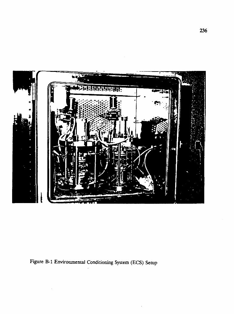
236
61110%,- lob
Figure B-1 Environmental Conditioning System (ECS) Setup
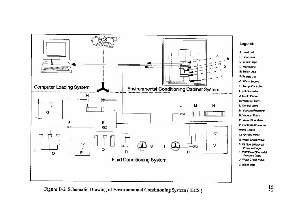
Computer Loading System
G
J K
Environmental Conditioning Cabinet System
PQ
R
L M N
DE
T
Fluid Conditioning System
Figure B-2 Schematic Drawing of Environmental Conditioning System ( ECS )
Legend:
A Load Cell
B: Specimen
C: Strain Gage
D: Membrane
E: Teflon Disk
F: Triaxial Cell
G: Water Source
H: Temp.-Controller
I : pH-Controller
J: Control Valve
K Water-Air Valve
L Control Valve
M: Vacuum Regulator
N: Vacuum Pump
0: Water Flow Meter
P: Controlled Pressure
Water Source
0: Air Flow Meter
R: Water Check Valve
S: IN Flow DifferentailPressure Gage
T: OUT Flow DifferentialPressure Gage
U: Water Check Valve
V: Water Trap
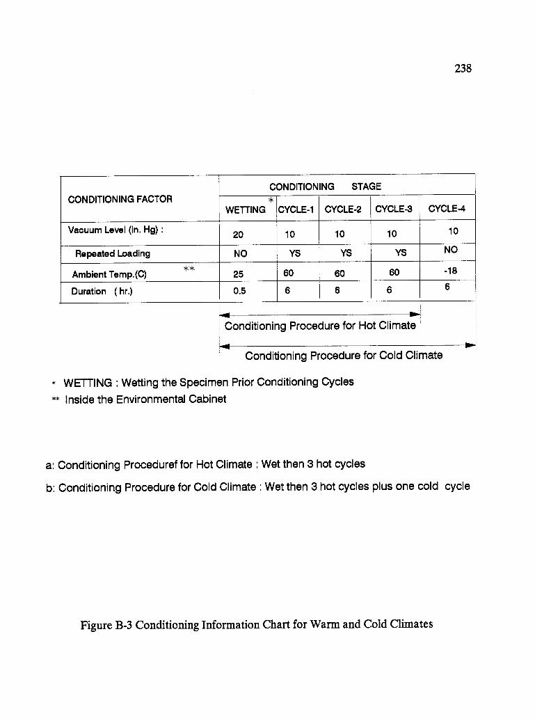
238
CONDITIONING FACTORCONDITIONING STAGE
*WETTING CYCLE-1 CYCLE-2 CYCLE-3 CYCLE-4
Vacuum Level (in. Hg) : 20 10 10 10 10
Repeated Loading NO YS YS YS NO
Ambient Temp.(C)**
25 60 60 60 -18
Duration ( hr.) 0.5 6 6 6 6
-41
Conditioning Procedure for Hot Climate
.41Conditioning Procedure for Cold Climate
WETTING : Wetting the Specimen Prior Conditioning Cycles
** Inside the Environmental Cabinet
00-
a: Conditioning Proceduref for Hot Climate : Wet then 3 hot cycles
b: Conditioning Procedure for Cold Climate : Wet then 3 hot cycles plus one cold cycle
Figure B-3 Conditioning Information Chart for Warm and Cold Climates
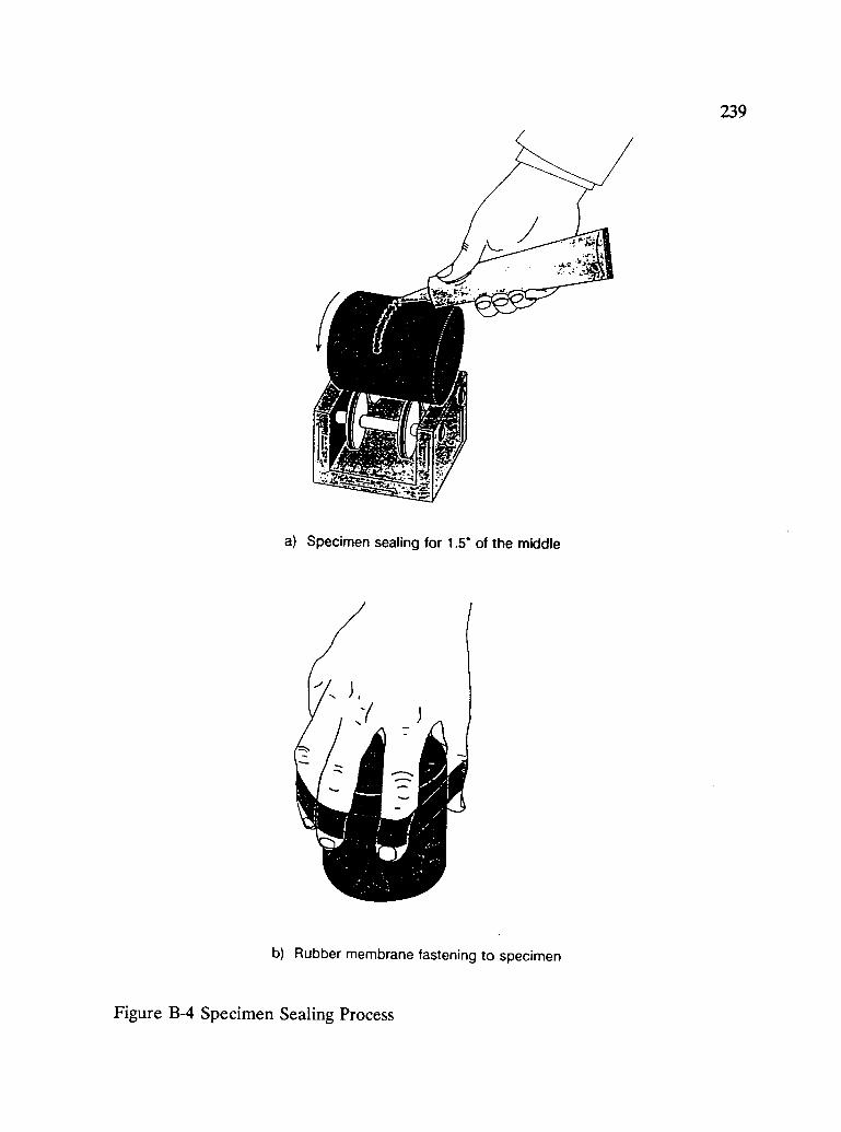
239
a) Specimen sealing for 1.5' of the middle
b) Rubber membrane fastening to specimen
Figure B-4 Specimen Sealing Process

240
(a) TOP VIEW OF TOP CAP
DRAINAGE HOLE
3/16 in. WIDE X 3/32 in.deep grooves
(b) GROOVE PATTERN FOR BOTTTOM OFTOP CAP AND TOP OF THE BASE
(c) PERFORATION PATTERN FOR TEFLON DISK
( 2/16" HOLE DIAMETER )
Figure B-5 Specimen End Platens and Teflon Disk Perforation Pattern
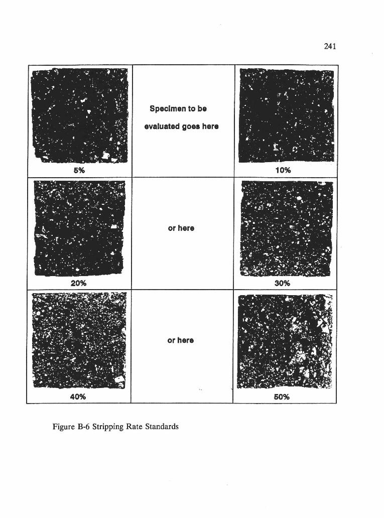
0
U)
.
,.1/1 ,
O
Oco)
OU)
O
242
APPENDIX C
WET CONDITIONING PROTOCOL
Scope
This conditioning procedure covers assembly set-ups, as well as wetting conditioningof compacted bituminous mixtures. Wet conditioning a specimen is defined as"pulling" water through the specimen at 20 in. Hg of vacuum for 30 minutes.Ambient room temperature is acceptable for both water and specimen.
Applicable Documents
AASHTO Standards:T 166 Bulk Specific Gravity of Compacted Bituminous MixturesT 167 Compressive Strength of Bituminous MixturesT 168 Sampling Bituminous MixturesT 209 Maximum Specific Gravity of Bituminous Paving MixturesT 247 Preparation of Test Specimens of Bituminous Mixtures by Means of
California Kneading Compactor or Gyratory CompactorT 269 Percent Air Voids in Compacted Dense and Open Bituminous Paving
Mixtures
Significance and Use
As noted in the scope, this method is intended to accelerate water conditioning ofcompacted bituminous mixtures in the laboratory. This method can be used to (a)test bituminous mixtures in conjunction with mixture design testing, or (b) testasphalt concrete cores and beams obtained from in-service pavements.

243
test bituminous mixtures in conjunction with mixture design testing, or (b) testasphalt concrete cores and beams obtained from in-service pavements.
Apparatus
According to the geometry of the test specimens there are two types of mold-specimen assembly setups. Figure C-1 shows the recommended mold-specimenassembly setup for cylindrical specimens, such as those prepared by Hveem kneadingcompactor.
Figure C-2 shows a suggested universal mold-specimen assembly setup for a beamspecimen which is adjustable to fit a range of expected beam sizes. Figure C-3 showsanother option for mold-specimen assembly set-up for a beam specimen. Figure C-4is a schematic sketch of a simplified wet conditioning system to be used with any ofthe specimen holders.
Preparation of Laboratory Test Specimens
See Apendix D.
Evaluation of Test Specimens and Grouping
See Appendix D.
Sealing the Test Specimen
As proposed earlier, this conditioning procedure is applicable for the two types ofspecimen geometries, cylindrical and beam specimens.
Leakage of water or air through the surface void system of cylindrical specimen(along the cylindrical surface of the specimen) when flow is being measured wouldgive erroneous results. Using a single seal at the mid-point was adequate.
To seal the cylindrical specimen use the following steps:
1. Place the specimen on specimen holder and apply silicon cement in themiddle of the specimen wall. Apply a large enough bead of siliconecement such that a surface 1.5 in. high is uniformly covered. Placea cylindrical rubber membrane of the same width (1.5 inches) over the
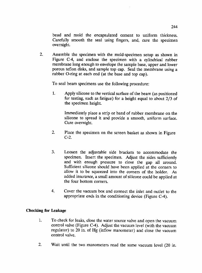
244
bead and mold the encapsulated cement to uniform thickness.Carefully smooth the seal using fingers, and, cure the specimenovernight.
2. Assemble the specimen with the mold-specimen setup as shown inFigure C-4, and enclose the specimen with a cylindrical rubbermembrane long enough to envelope the sample base, upper and lowerporous teflon disks, and sample top cap. Seal the membrane using arubber 0-ring at each end (at the base and top cap).
To seal beam specimens use the following procedure:
1. Apply silicone to the vertical surface of the beam (as positionedfor testing, such as fatigue) for a height equal to about 2/3 ofthe specimen height.
Immediately place a strip or band of rubber membrane on thesilicone to spread it and provide a smooth, uniform surface.Cure overnight.
2. Place the specimen on the screen basket as shown in FigureC-2.
3. Loosen the adjustable side brackets to accommodate thespecimen. Insert the specimen. Adjust the sides sufficientlyand with enough pressure to close the gap all around.Sufficient silicone should have been applied at the corners toallow it to be squeezed into the corners of the holder. Asadded insurance, a small amount of silicone could be applied atthe four bottom corners.
4. Cover the vacuum box and connect the inlet and outlet to theappropriate ends in the conditioning device (Figure C-4).
Checking for Leakage
1. To check for leaks, close the water source valve and open the vacuumcontrol valve (Figure C-4). Adjust the vacuum level (with the vacuumregulator) to 20 in. of Hg (inflow manometer) and close the vacuumcontrol valve.
2. Wait until the two manometers read the same vacuum level (20 in.
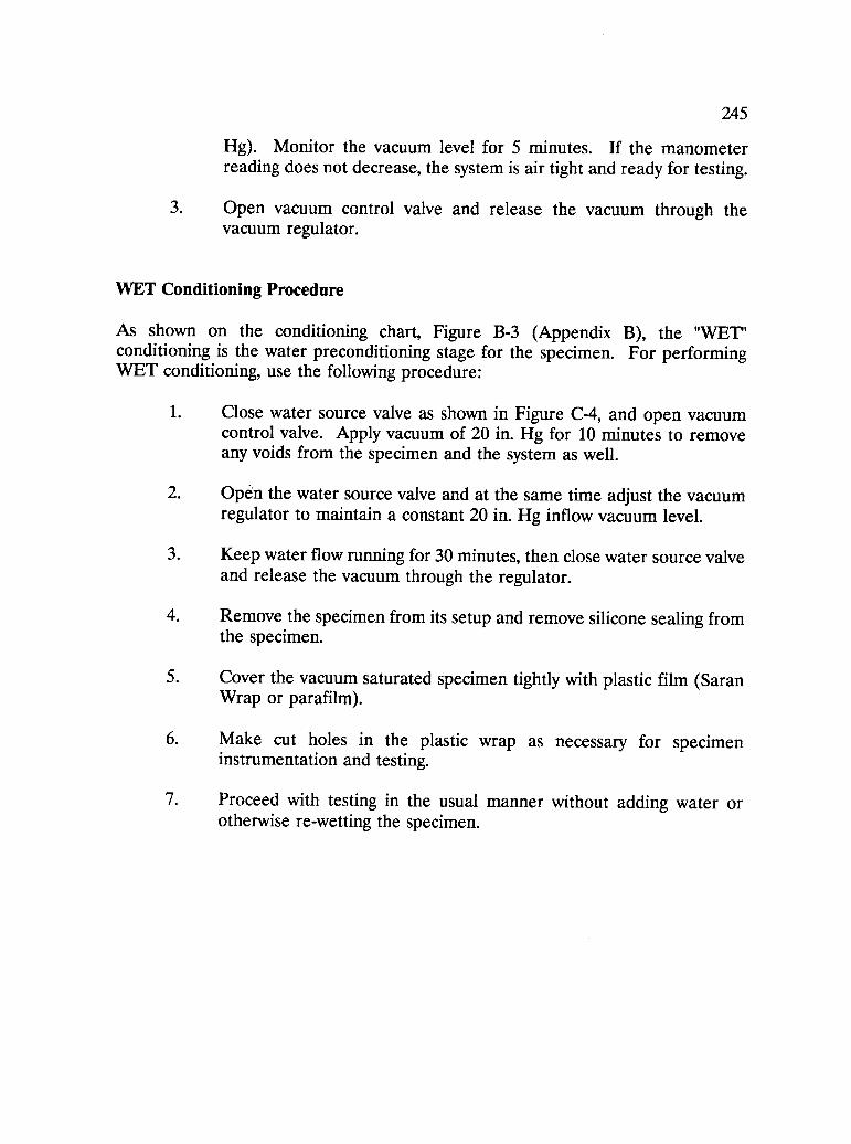
245
Hg). Monitor the vacuum level for 5 minutes. If the manometerreading does not decrease, the system is air tight and ready for testing.
3. Open vacuum control valve and release the vacuum through thevacuum regulator.
WET Conditioning Procedure
As shown on the conditioning chart, Figure B-3 (Appendix B), the "WET"conditioning is the water preconditioning stage for the specimen. For performingWET conditioning, use the following procedure:
1. Close water source valve as shown in Figure C-4, and open vacuumcontrol valve. Apply vacuum of 20 in. Hg for 10 minutes to removeany voids from the specimen and the system as well.
2. Open the water source valve and at the same time adjust the vacuumregulator to maintain a constant 20 in. Hg inflow vacuum level.
3. Keep water flow running for 30 minutes, then close water source valveand release the vacuum through the regulator.
4. Remove the specimen from its setup and remove silicone sealing fromthe specimen.
5. Cover the vacuum saturated specimen tightly with plastic film (SaranWrap or parafilm).
6. Make cut holes in the plastic wrap as necessary for specimeninstrumentation and testing.
7. Proceed with testing in the usual manner without adding water orotherwise re-wetting the specimen.
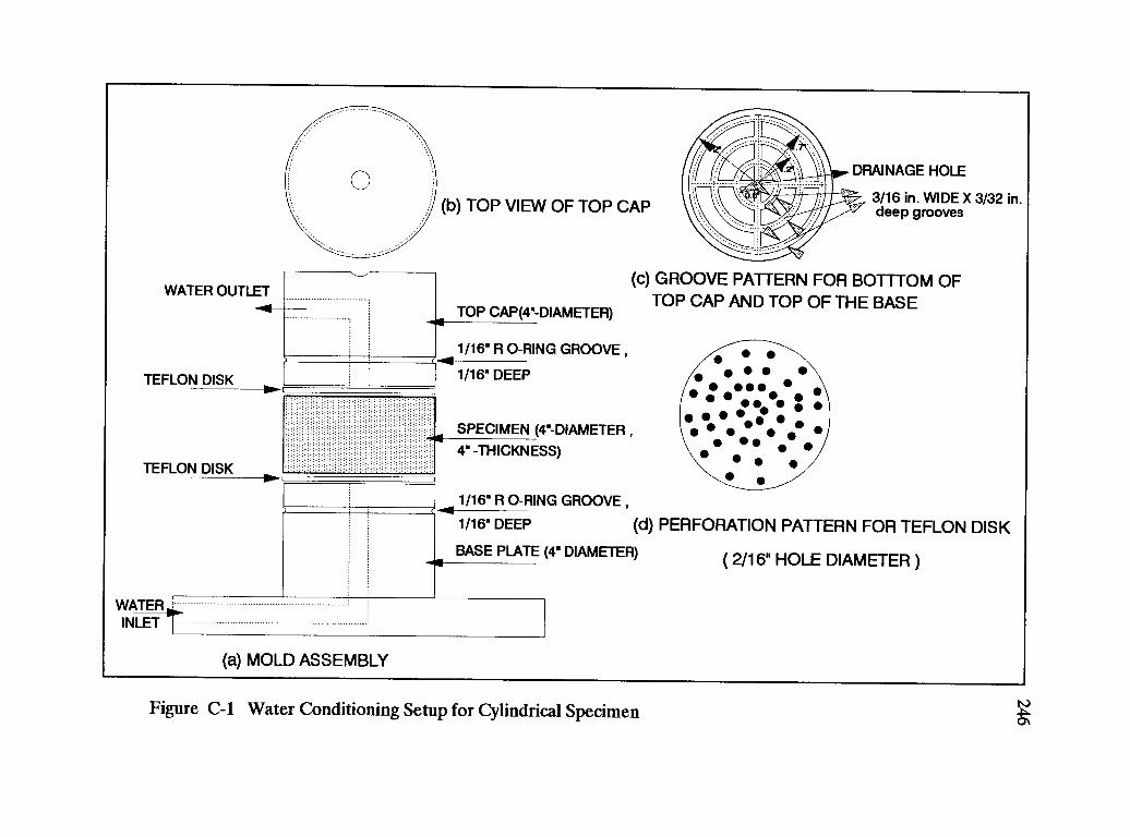
WATER OUTLET
TEFLON DISK
TEFLON DISK
WATERINLET
(b) TOP VIEW OF TOP CAP
TOP CAP(4"-DIAMETER)
1/16" R 0-RING GROOVE ,
1 /1 6" DEEP
DRAINAGE HOLE
3/16 in. WIDE X 3/32 in.deep grooves
(c) GROOVE PATTERN FOR BOTTTOM OFTOP CAP AND TOP OF THE BASE
SPECIMEN (4"-DIAMETER ,
4" -THICKNESS)
:00 lb.
ga
1/16" R 0-RING GROOVE ,
1/16" DEEP (d) PERFORATION PATTERN FOR TEFLON DISK
BASE PLATE (4" DIAMETER) ( 2/16" HOLE DIAMETER )
(a) MOLD ASSEMBLY
Figure C-1 Water Conditioning Setup for Cylindrical Specimen
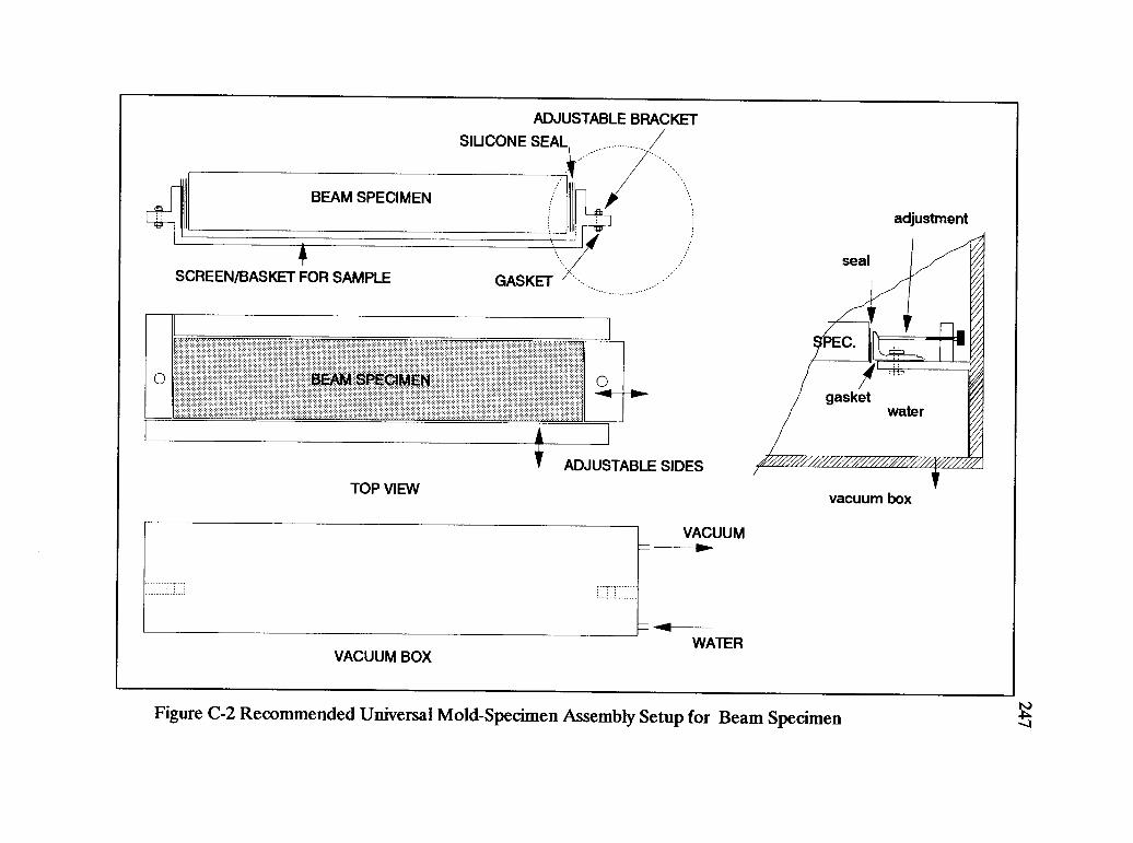
-.111111-10.-
ADJUSTABLE BRACKET
SIUCONE SEAL
BEAM SPECIMEN
SCREEN/BASKET FOR SAMPLE GASKET
0 SEAM SPECIMEN
ADJUSTABLE SIDES
TOP VIEW
VACUUM BOX
VACUUM
WATER
adjustment
vacuum box
Figure C-2 Recommended Universal Mold-Specimen Assembly Setup for Beam Specimen
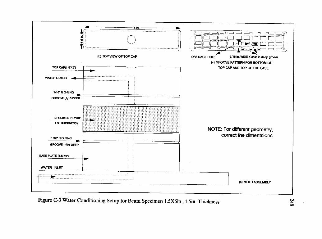
A
TOP CAP(1.51(6)
6 in.
(b) TOP VIEW OF TOP CAP
WATER OUTLET -.11
1/16' R 0-RING
GROOVE ,1/16 DEEP
SPECIMEN (1.5X6',
1.6 THICKNESS)
1/16 R 0-RING
GROOVE ,1/16 DEEP
BASE PLATE (1.51(61
WATER INLET
I I 1 I I I I II I I I I 1 I 1
I I I 1 iir I 1 1 I
DRAINAGE HOLE 3/16 in. WIDE X 3/32 in.deep groove
(c) GROOVE PATTERN FOR BOTTOM OF
TOP CAP AND TOP OF THE BASE
NOTE: For different geometry,correct the dimentsions
(a) MOLD ASSEMBLY
Figure C-3 Water Conditioning Setup for Beam Specimen 1.5X6in , 1.5in. Thickness
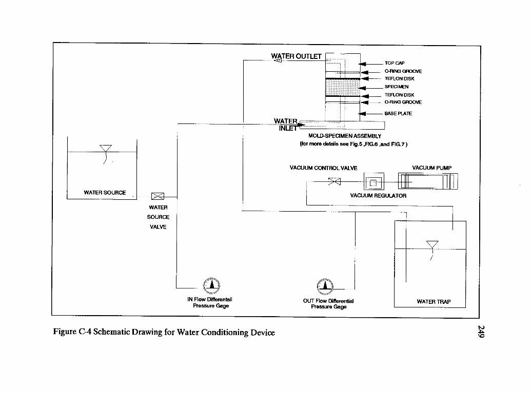
WATER SOURCE >1WATER
SOURCE
VALVE
IN Flow Differentail
VVTER OUTLETTOP CAP
0-RING GROOVE
TEFLON DISK
SPECIMEN
TEFLON DISK
0-RING GROOVE
WAILER*.IN
MOW-SPECIMEN ASSEMBLY
(for more details see Fig.5 ,FIG.6 And FIG.7 )
BASE PLATE
VACUUM CONTROL VALVE VACUUM PUMP
XI Et
VACUUM REGULATOR
oOUT Flow Differential
Pressure Gage Pressure GageWATER TRAP
Figure C-4 Schematic Drawing for Water Conditioning Device W

250
APPENDIX D
SAMPLE PREPARATION PROTOCOL
Preparation of Laboratory Test Specimens
1. Specimens 4-in. (102 mm) in diameter and 4-in. (63.5 mm) high arenormally used. Specimens of larger dimensions may be used if desiredand should be used if aggregate larger than 1-in. (25.4 mm) is presentin the mixture and/or is not permitted to be scalped out.
2. After mixing, the mixture shall be placed in an aluminum pan havinga surface area of 75-100 square inches in the bottom and a depth ofapproximately 1-in. (25.4 mm) and cooled at room temperature for 2± 0.5 hours. Then the mixture shall be placed in a 140°F (60°C) ovenfor 16 hours for curing. The pans should be placed on spacers to allowair circulation under the pan if the shelves are not perforated.
3. After curing, place the mixture in an oven at 275 °F (135 °C) for 2hours prior to compaction. The mixture shall be compacted in twolifts. Desired air void level can be obtained by adjusting the footpressure, number of tamps, levelling load, or some combination inAASHTO T247; or number of revolutions in ASTM D 3387. Theexact procedure must be determined experimentally for each mixturebefore compacting the specimens for each set.
4. After extraction from the molds, the test specimens shall be stored for72 to 96 hours at room temperature.

251
Evaluation of Test Specimens and Grouping
1. Determine theoretical maximum specific gravity of the mixture byAASHTO T-209.
2. Determine specimen thickness by ASTM D 3549.
3. Determine bulk specific gravity by ASTM D 2726 and ASTM D 1188.The determination of the bulk specific gravity of compacted asphaltconcrete specimens is to be done according to ASTM D 1188(replacing paraffin coating by parafilm wrapping). According to thecomparative study at OSU, for calculating air voids by the regularmethod ASTM D 2726 (based on the weight of saturated surface-dryspecimen in air) and using parafilm for ASTM D 1188, there is adifference between the two methods; where the results (air voids) byparafilm are about 1.5% higher than those results without parafilm(ASTM D 2726), according to aggregate type. In order to insureconsistency in determination of bulk specific gravity by differentlaboratories involved with the SHRP A-003A project, bulk specificgravity will be determined by both methods: one by using the parafilmwith ASTM D 1188 and the second by using regular method ASTMD 2726.
4. Calculate air voids by AASHTO T-289. Percent air void levels 4, 8,and 20%, will be based on the bulk specific gravity calculated byASTM D 1188.
Sealing the Test Specimen
1. Place the specimen on specimen holder and apply silicone cement inthe middle of the specimen wall. Apply a large enough bead ofcement such that a surface 1.5 inches high is uniformly covered. Placea cylindrical rubber membrane of the same width (1.5 inches) over thebead of cement and mold the encapsulated cement to uniformthickness using your fingers. Cure the specimen overnight.
2. Place the specimen in the triaxial apparatus and complete all electricalconnections (i.e., LVDs and load cell.) Envelope the specimen with
252
a cylindrical rubber membrane long enough to envelope the samplebase, the upper and lower porous teflon disks, and the sample top cap.Seal the membrane using rubber 0-rings at each end (at the base andtop cap.)
3. Attach the vacuum outlet to the manometer and vacuum pump, andto the inlet of the flowmeter.
253
APPENDIX E
RESISTANCE OF COMPACTED BITUMINOUS MIXTURE TO MOISTUREINDUCED DAMAGE
AASHTO DESIGNATION: T 283-85Modified for use at OSU under SHRP contract A-003A
1.1 Scope
This method covers preparation of specimens and measurement of the change ofdiametral tensile strength and diametral resilient modulus resulting from the effectsof saturation and accelerated water conditioning of compacted bituminous mixtures.Internal water pressures in the compacted specimens are produced by vacuumsaturation followed by a freeze and thaw cycle. Two numerical indices of retainedindirect tensile strength and resilient modulus are obtained by comparing the valuesbefore and after conditioning.
Applicable Documents
AASHTO Standards:
T 166 Bulk Specific Gravity of Compacted Bituminous MixturesT 167 Compressive Strength of Bituminous MixturesT 168 Sampling Bituminous Paving MixturesT 209 Maximum Specific Gravity of Bituminous Paving MixturesT 245 Resistance to Plastic Flow of Bituminous Mixtures Using
254
T 245 Resistance to Plastic Flow of Bituminous Mixtures UsingMarshall Apparatus
T 246 Resistance to Deformation and Cohesion of BituminousMixtures by Means of Hveem Apparatus
T 247 Preparation of Test Specimens of Bituminous Mixtures byMeans of California Kneading Compactor
T 269 Percent Air Voids in Compacted Dense and Open BituminousPaving Mixtures
M 156 Requirements for Mixing Plants for Hot-Mixed, Hot-Laid Bituminous Paving Mixtures
ASTM Standards:
D 3387 Test for Compaction and Shear Properties of BituminousMixtures by Means of the U.S. Corps of EngineersGyratory Testing Machine (GTM)
D 3549 Test for Thickness or Height of Compacted BituminousPaving Mixture Specimens
D 4123 Indirect Tension Test for Resilient Modulus ofBituminous Mixtures
Significance and Use
As noted in the scope, this method is intended to evaluate the effects of saturationand accelerated water conditioning of compacted bituminous mixtures in thelaboratory. This method can be used (a) to test bituminous mixtures in conjunctionwith mixture design testing, (b) to test bituminous mixtures produced at mixingplants, and (c) to test the bituminous concrete cores obtained from completedpavements of any age.
Numerical indices of retained indirect tensile properties are obtained by comparingthe retained indirect properties of saturated, accelerated water-conditioned laboratoryspecimens with the similar properties of dry specimens.
Summary of Method
Six test specimens for each set of mix conditions, such as plain asphalt, asphalt withantistripping agent, and aggregate treated with lime, are tested (Note 1). Each setof specimens is divided into and tested in a dry condition for resilient modulus. The
1 - It is recommended to prepare two additional specimens for the set. These specimens can then beused to establish the vacuum saturation technique.
255
other set is subjected to vacuum saturation followed by a freeze and warm-watersoaking cycle and then tested for resilient modulus and tensile strength. Twonumerical indices of retained resilient modulus and tensile strength are computedfrom the test data obtained on the two subsets: dry and conditioned.
Apparatus
Equipment for preparing and compacting specimens from one of the followingAASHTO Methods: T 245 and T 247, or ASTM Method D 3387.
Vacuum Container, preferably Type D, from ASTM Method D 2041 and vacuumpump or water aspirator from ASTM D 2041 including manometer or vacuum gauge.
Balance and water bath from AASHTO T 166.
Water bath capable of maintaining a temperature of 140° ± 1.8°F (60 ± 1°C).
Freezer maintained at 0 ± 5 °F (-18° ± 3 °C).
A supply of plastic film for wrapping, heavy-duty leak proof plastic bags to enclosethe saturated specimens and masking tape.
10 ml graduated cylinder.
Aluminum pans having a surface area of 75-100 square inches in the bottom and adepth of approximately 1 inch.
Forced air draft oven capable of maintaining a temperature of 140° ± 1.8°F (60°± 1°C).
Apparatus as listed in ASTM D 4123.
Preparation of Laboratory Test Specimens
Specimens 4 inches (102 mm) in diameter and 2.5 inches (63.5 mm) high are usuallyused. Specimens of larger dimensions may be used if desired and should be used ifaggregate larger than 1 inch (25.4 mm) is present in the mixture and/or is notpermitted to be scalped out.
After mixing, the mixture shall be placed in an aluminum pan having a surface areaof 75-100 square inches in the bottom and a depth of approximately 1 inch (25.4 mm)and cooled at room temperature for 2 ± 0.5 hours. Then the mixture shall be placed
256
in a 140°F (60°C) oven for 16 hours for curing. The pans should be placed onspacers to allow air circulation under the pan if the shelves are not perforated.
After curing, place the mixture in an oven at 275 °F (135 °C) for 2 hours prior tocompaction. The mixture shall be compacted to 7 ± 1.0 percent air voids or a voidlevel expected in the field. This level of voids can be obtained by adjusted thenumber of blows in AASHTO T 245; adjusting foot pressure, number of tamps,levelling load, or some combination in AASHTO T 247; and adjusting the numberof revolutions in ASTM D 3387. The exact procedure must be determinedexperimentally for each mixture before compacting the specimens for each set.
After extraction from the molds, the test specimens shall be stored for 72 to 96 hoursat room temperature.
Preparation of Core Test Specimens
Select locations on the completed pavement to be sampled, and obtain cores. Thenumber of cores shall be at least 6 for each set of mix conditions.
Separate core layers as necessary by sawing or other suitable means, and store layersto be tested at room temperature.
Evaluation of Test Specimens and Grouping
Determine theoretical maximum specific gravity by mixture by AASHTO T 209.
Determine specimen thickness by ASTM D 3549.
Determine bulk specific gravity by D 2726 and D 1188. In order to ensureconsistency in determination of bulk specific gravity by different laboratories involvedwith the SHRP A003A project, bulk specific gravity will be determined by the twomethods. One by using the parafilm with D 1188, only for air voids determinationfor dry specimens, and the second by using regular method D 2726, for all the threecircumstances (dry, saturated, and water-conditioned specimens). Continuously drainwater, which makes it very difficult to wrap the specimen with parafilm within therequired short time period.
Calculate air voids by AASHTO T 269. Target air voids (6 8%) will be based onthe bulk specific gravity calculated by D 2726.
Sort specimens into two subsets of three specimens each so that average air voids ofthe two subsets are approximately equal.
257
Preconditioning of Test Specimens
At least six specimens shall be made for each test, three to be tested dry and threeto be tested after saturation and water conditioning. The average air voids of thetwo subsets are approximately equal.
Specimens 4 inches in diameter and 2.5 inches high are used. Specimens of greaterdimensions may be used if desired and should be used if aggregate larger than 1 inchis present.
The dry subset will be tested as follows:
1. Determine the permeability as described in Appendix F
2. For bringing dry specimens to tensile strength and resilient modulustest temperatures without water intrusion into the dry specimens in thewater bath, we need to enclose the dry specimens in heavy duty leak -proof plastic bags or we can use metal jars of at least 4 inches in
diameter and at least 6 inches high. In this study we use controlledtemperature cabinet.
3. If only low-to-moderate stresses are applied to the specimens in thediametral resilient modulus test, this test can be considerednondestructive and the same specimens can be used for the diametraltensile strength test. Since they will be used for the two subsets,specimens should be maintained at test temperature either to beenclosed in the controlled temperature cabinet for dry specimen or tobe re- immersed in the water bath, for conditioned specimens, atselected test temperature 77°F (25 °C) for 1 to 2 hours after diametralresilient modulus testing and prior to the diametral tensile strengthtesting.
4. The second subset shall be conditioned as follows:
Place the specimens in the vacuum container. The specimenswill be supported above the container bottom by a spacer. Fillthe container with distilled water at room temperature so thatthe specimens have at least 1 inch of water above their surface.Apply partial vacuum by either attaching a vacuum hose fromvacuum pump or a water aspirator as was used at OSU. Apply
258
the partial vacuum, such as 20 inches Hg, for a short time, suchas five minutes. The level of vacuum and time duration appearto be different for different mixtures, but the vacuum level ismore effective in changing the degree of saturation than thetime duration. Remove the vacuum and leave the specimenssubmerged in water for 30 minutes.
Remove each of the specimens from the vacuum container,surface dry the specimen by blotting quickly with a damp towel(regardless of the water draining from specimen) and weighimmediately in air. This is the saturated surface dry weight forsaturated specimen. Then weigh the specimen submerged indistilled water bath at 77 °F (25 ° C) to get weight in water forsaturated specimen. Immediately after weighing eachsubmerged specimen, return the specimens to the water-filledvacuum container and submerge each specimen temporarilyunder the water at atmospheric pressure.
Determine specimen thickness by Method D 3549.
Calculate volume of absorbed water by subtracting the air dryweight of the specimen found in section 8.3.
Determine the degree of saturation by dividing the volume ofabsorbed water by the volume of air voids and express theresult as a percentage. If this percentage is between 55 and 80,proceed the test. If it is more than 80 percent the specimen hasbeen damaged and is discarded. If calculated percentage is lessthan 55 percent, repeat the procedure beginning with newspecimen using a slightly higher partial vacuum.
Determine the ratio of volume change (in most circumstances,this will be swell) of saturated specimens by dividing the changein specimen volume found in saturated specimen and dryspecimen volume by the dry specimen volume.
Cover the vacuum saturated specimens tightly with plastic film(saran wrap or equivalent). Place each wrapped specimen in aplastic bag containing 10 ml of distilled water and seal the bag.
Place the plastic bag containing specimen in a freezer at 0° +5 °(-18 ° + 3 °) for 16 hours.
After 16 hours, take the specimens from the freezer and remove
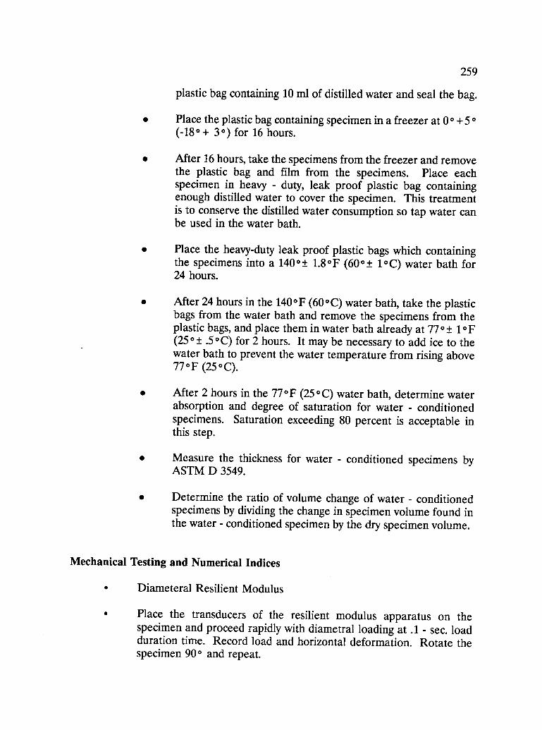
259
plastic bag containing 10 ml of distilled water and seal the bag.
Place the plastic bag containing specimen in a freezer at 0° +5°(-18 ° + 3°) for 16 hours.
After 16 hours, take the specimens from the freezer and removethe plastic bag and film from the specimens. Place eachspecimen in heavy duty, leak proof plastic bag containingenough distilled water to cover the specimen. This treatmentis to conserve the distilled water consumption so tap water canbe used in the water bath.
Place the heavy-duty leak proof plastic bags which containingthe specimens into a 140 ° ± 1.8°F (60 ° ± 1°C) water bath for24 hours.
After 24 hours in the 140°F (60°C) water bath, take the plasticbags from the water bath and remove the specimens from theplastic bags, and place them in water bath already at 77° ± 1°F(25 ° ± .5 °C) for 2 hours. It may be necessary to add ice to thewater bath to prevent the water temperature from rising above77°F (25 ° C).
After 2 hours in the 77°F (25°C) water bath, determine waterabsorption and degree of saturation for water - conditionedspecimens. Saturation exceeding 80 percent is acceptable inthis step.
Measure the thickness for water - conditioned specimens byASTM D 3549.
Determine the ratio of volume change of water conditionedspecimens by dividing the change in specimen volume found inthe water - conditioned specimen by the dry specimen volume.
Mechanical Testing and Numerical Indices
Diameteral Resilient Modulus
Place the transducers of the resilient modulus apparatus on thespecimen and proceed rapidly with diametral loading at .1 - sec. loadduration time. Record load and horizontal deformation. Rotate thespecimen 90° and repeat.
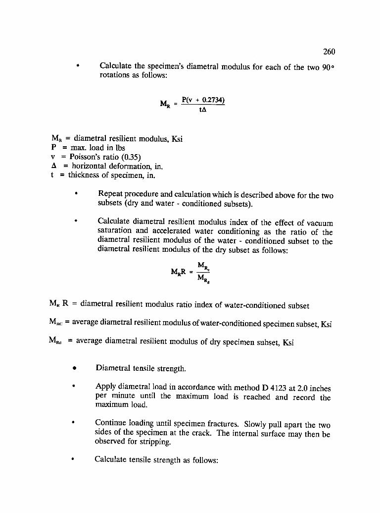
260
Calculate the specimen's diametral modulus for each of the two 90°rotations as follows:
MRto
P(v + 0.2734)
MR = diametral resilient modulus, KsiP = max. load in lbsv = Poisson's ratio (0.35)A = horizontal deformation, in.t = thickness of specimen, in.
Repeat procedure and calculation which is described above for the twosubsets (dry and water - conditioned subsets).
Calculate diametral resilient modulus index of the effect of vacuumsaturation and accelerated water conditioning as the ratio of thediametral resilient modulus of the water - conditioned subset to thediametral resilient modulus of the dry subset as follows:
MM RR la;
Rd
MR R = diametral resilient modulus ratio index of water-conditioned subset
MRC = average diametral resilient modulus of water-conditioned specimen subset, Ksi
MRd = average diametral resilient modulus of dry specimen subset, Ksi
Diametral tensile strength.
Apply diametral load in accordance with method D 4123 at 2.0 inchesper minute until the maximum load is reached and record themaximum load.
Continue loading until specimen fractures. Slowly pull apart the twosides of the specimen at the crack. The internal surface may then beobserved for stripping.
Calculate tensile strength as follows:
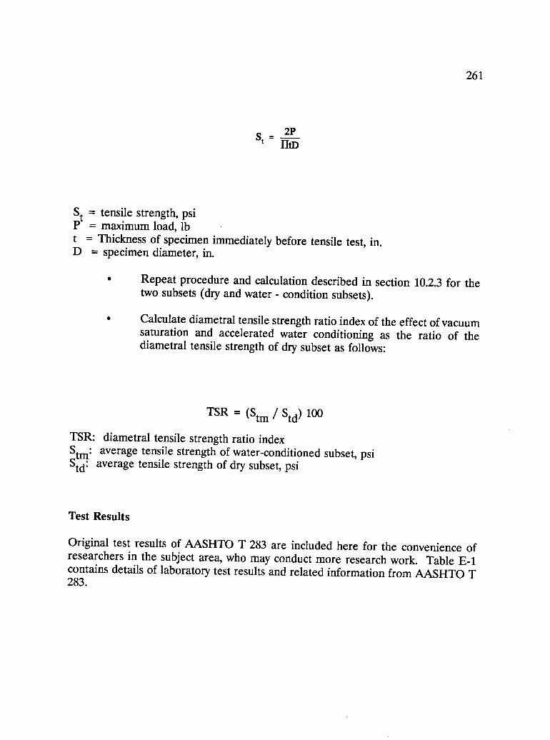
261
2PS` = rid)
St = tensile strength, psiP = maximum load, lbt = Thickness of specimen immediately before tensile test, in.D = specimen diameter, in.
Repeat procedure and calculation described in section 10.2.3 for thetwo subsets (dry and water - condition subsets).
Calculate diametral tensile strength ratio index of the effect of vacuumsaturation and accelerated water conditioning as the ratio of thediametral tensile strength of dry subset as follows:
TSR = (Stm / Std) 100
TSR: diametral tensile strength ratio indexStm: average tensile strength of water-conditioned subset, psiStd: average tensile strength of dry subset, psi
Test Results
Original test results of AASHTO T 283 are included here for the convenience ofresearchers in the subject area, who may conduct more research work. Table E-1contains details of laboratory test results and related information from AASHTO T283.
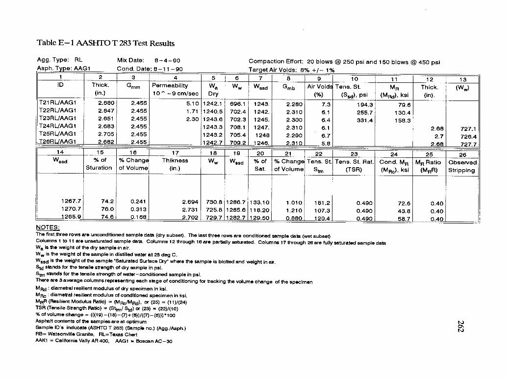
Table E- 1 AASHTO T 283 Test Results
Agg. Type: RLAs h. T e: AAG1
Mix Date: 8-4-90Cond. Date: 8-11-90
Compaction Effort: 20 blows @ 250 psi and 150 blows @ 450 psiTarget Air Voids: 8% +/- 1%
1 2 3 4 5 6 7 8 9 10 11 12 13ID Thick. Gmm Permeability Wa Ww Wssd Gmb Air Voids Tens. St. MR Thick. (Ww)
(in.) 10 ^ -9 cm/sec Dry (%) (Ssd), psi (MRd), ksi (in).T21RL/AAG1 2.680 2.455 5.10 1242.1 696.1 1243. 2.280 7.3 194.3 79.6T22RL/AAGI 2.647 2.455 1.71 1240.5 702.4 1242. 2.310 6.1 255.7 130.4T23RL/AAG1 2.651 2.455 2.30 1243.6 702.3 1245. 2.300 6.4 331.4 158.3T24RL/AAG1 2.683 2.455 1243.3 708.1 1247. 2.310 6.1 2.68 727.1T25RL1AAG1 2.705 2.455 1243.2 705.4 1248 2.290 6.7 2.7 726.4T26RL/AAG1 2.682 2.455 1242.7 709.2 1246. 2.310 5.8 2.68 727.7
14 15 16 17 18 19 20 21 22 23 24 25 26Wssd % of % Change Thikness Ww Wssd % of % Change Tens. St. Tens. St. Rat. Cond. MR MR Ratio Observed
Sturation of Volume (in.) Sat. of Volume S" (TSR) (Mild, ksi (MRR) Stripping
1267.7 74.2 0.241 2.694 730.8 1286.7 133.10 1.010 181.2 0.490 72.6 0.401270.7 76.0 0.313 2.731 725.8 1285.6 118.20 1.210 107.3 0.490 43.8 0.401265.9 74.6 0.168 2.702 729.7 1282.7 129.50 0.880 120.4 0.490 58.7 0.40
NOTES:The first three rows are unconditioned sample data (dry subset). The last three rows are conditioned sample data (wet subset)Columns 1 to 11 are unsaturated sample data. Columns 12 through 16 are partially saturated. Columns 17 through 26 are fully saturated sample dataWa is the weight of the dry sample in air.Ww is the weight of the sample in distilled water at 25 deg C.Wssd is the weight of the sample "Saturated Surface Dry" where the sample is blotted and weight in air.Std stands for the tensile strength of dry sample in psi.San stands for the tensile strength of water-conditioned sample in psi.There are 3 average columns representing each stage of conditioning for tracking the volume change of the specimenMRd : diametral resilient modulus of dry specimen in ksi.MRa : diametral resilient modulus of conditioned specimen in ksi.MRR (Resilient Modulus Ratio) = (MRb/MRd), or (25) = (11)/(24)TSR (Tensile Strength Ratio) = (Stan/ Std) or (23) = (22)/(10)% of volume change = (((19) -(18)- (7)+(6))/((7)- (6)))*100Asphalt contents of the samples are at optimumSample ID's inducate (ASHTO T 283) (Sample no.) (Agg./Asph.)RB= Watsonville Granite, RL=Texas ChertAAK1 = California Vally AR 400, AAG1 = Boscan AC-30

Table E- 1 (Continued)
Agg. Type: RLAs h. Type: AAG1
Mix Date: 5-13-90Cond. Date: 8-15-90
Compaction Effort: 20 blows @ 250 psi and 150 blows @ 450 psiTarget Air Voids: 8% +/- 1%
1 2 3 4 5 6 7 8 9 10 11 12 13ID Thick. G Permeability Wa Ww Wssd Gmb Air Voids Tens. St. MR Thick. (Ww)
(in.) 10 ^ -9 cm/sec Dry (%) (Ssd), psi (MRd), ksi (in).T29RL/AAG1 2.663 2.475 0.16 1238.6 696.7 1240. 2.287 7.6 427.7 181.7T33RL/AAG1 2.651 2.475 0.20 1244.5 708.1 1246. 2.321 6.2 543.9 210.7T31RL/AAG1 2.660 2.475 0.24 1241.6 700.0 1243. 2.293 7.3 464.4 173.9T32RL/AAG1 2.656 2.475 1243.8 715.3 1279. 2.328 5.9 2.658 730.2T3ORL/AAG1 2.637 2.475 1237.4 706.6 1245. 2.297 7.2 2.648 726T34RL/AAG1 2.697 2.475 1239.9 706.8 1241. 2.319 6.3 2.701 726.9
14 15 16 17 18 19 20 21 22 23 24 25 26Wssd % of % Change Thikness Ww Wssd % of % Change Tens. St. Tens. St. Rat. Cond. MR MR Ratio Observed
Sturation of Volume (in.) Sat. of Volume Stm (TSR) (MRa), ksi (MRR) Stripping
1264.5 65.4 0.019 2.669 733.7 1281.0 118.80 1.097 146.3 0.300 91.3 0.401262.6 65.0 -0.390 2.653 729.1 1279.8 111.10 1.093 147.2 0.300 65.7 0.401265.3 75.3 0.692 2.716 730.7 1283.5 129.60 0.994 167.8 0.300 76.0 0.40
NOTES:The first three rows are unconditioned sample data (dry subset). The last three rows are conditioned sample data (wet subset)Columns 1 to 11 are unsaturated sample data. Columns 12 through 16 are partially saturated. Columns17 through 26 are fully saturated sample dataWa is the weight of the dry sample in air.Ww is the weight of the sample in distilled water at 25 deg C.Wssd is the weight of the sample "Saturated Surface Dry" where the sample is blotted and weight in air.Std stands for the tensile strength of dry sample in psi.Sim stands for the tensile strength of water-conditioned sample in psi.There are 3 average columns representing each stage of conditioning for tracking the volume change of the specimenMRd : diametral resilient modulus of dry specimen in ksi.MRe : diametral resilient modulus of conditioned specimen in ksi.MRR (Resilient Modulus Ratio) = (MRa/MRd), or (25) = (11)/(24)TSR (Tensile Strength Ratio) = (Sttm/ Std) or (23) = (22)/(10)% of volume change = (((19) - (18)- (7)+(6))/((7)- (6)))*100Asphalt contents of the samples are at optimumSample ID's indurate (ASHTO T 283) (Sample no.) (Agg./Asph.)RB= Watsonville Granite, RL=Texas ChertAAK1 = California Vally AR 400, AAG1 = Boscan AC-30

Table E- 1 (Continued)
Agg. Type: RLAs h. T e: AAK1
Mix Date: 5-31 -90Cond. Date: 6-1-90
Compaction Effort: 20 blows @ 250 psi and 150 blows @ 450 psiTarget Air Voids: 8% +/- 1%
1 2 3 4 5 6 7 8 9 10 11 12 13ID Thick. Gmm Permeability Wa Ww Wssd Gmb Air Voids Tens. St. MR Thick. (Ww)
(in.) 10 ^ -9 cm/sec Dry ( %) (Ssd), psi (MRd), ksi (in).T36RL/AAK1 2.650 2.456 0.22 1241.9 705.7 1244.0 2.307 6.1 122.8T37RL/AAK1 2.687 2.456 0.19 1245.0 705.0 1247.3 2.296 6.5 121.1 166.8T35RL/AAK1 2.707 2.456 1244.2 694.1 1247.6 2.280 7.2 2.71 724.4T38RL/AAK1 2.693 2.456 1246.3 703.2 1246.2 2.287 6.9 2.69 728.5
14 15 16 17 18 19 20 21 22 23 24 25 26Wssd % of % Change Thikness Ww Wssd % of % Change Tens. St. Tens. St. Rat. Cond. MR MR Ratio Observed
Sturation of Volume (in.) Sat. of Volume Stm (TSR) (Mild), ksi (MAR) Stripping
1270.8 67.1 -1.300 2.713 726.0 1277.0 0.83 -0.670 72.0 0.542 162.6 0.741272.3 69.6 0.100 2.693 730.8 1284.1 1.01 0.130 60.3 0.542 84.4 0.74
NOTES:The first three rows are unconditioned sample data (dry subset). The last three rows are conditioned sample data (wet subset)Columns 1 to 11 are unsaturated sample data. Columns 12 through 16 are partially saturated. Columns17 through 26 are fully saturated sample dataWa is the weight of the dry sample in air.Ww is the weight of the sample in distilled water at 25 deg C.Wssd is the weight of the sample "Saturated Surface Dry" where the sample is blotted and weight in air.Std stands for the tensile strength of dry sample in psi.Stm stands for the tensile strength of water-conditioned sample in psi.There are 3 average columns representing each stage of conditioning for tracking the volume change of the specimenMRd : diametral resilient modulus of dry specimen in ksi.MRc : diametral resilient modulus of conditioned specimen in ksi.MAR (Resilient Modulus Ratio) = (MRc/MRd), or (25) = (11)/(24)TSR (Tensile Strength Ratio) = (Stall/ Std) or (23) = (22)/(10)% of volume change = (((19) - (18)- (7)+09)/07)- (6)))*1 00Asphalt contents of the samples are at optimumSample ID's inducate (ASHTO T 283) (Sample no.) (Agg./Asph.)RB= Watsonville Granite, RL=Texas ChartAAK1 = California Vally AR 400, AAG1 = Boscan AC-30
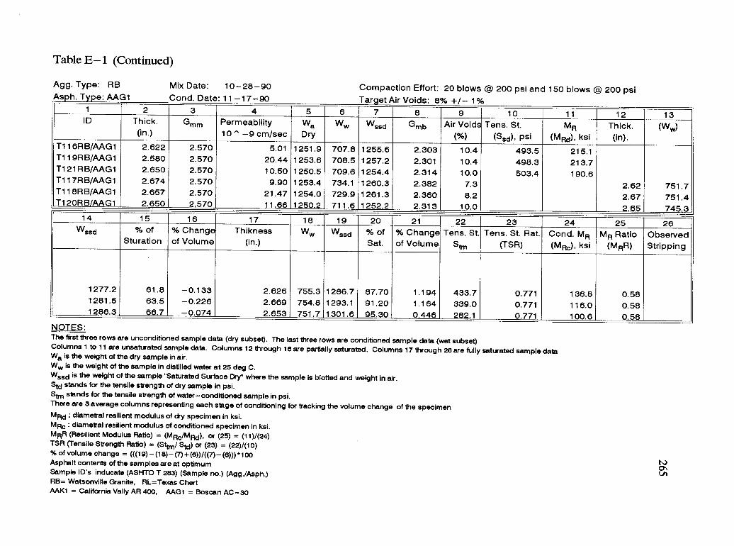
Table E- 1 (Continued)
Agg. Type: RBAs h. T e: AAG1
Mix Date: 10-28-90Cond. Date: 11-17-90
Compaction Effort: 20 blows @ 200 psi and 150 blows @ 200 psiTarget Air Voids: 8% +/- 1%
1 2 3 4 5 6 7 8 9 10 11 12 13ID Thick. Gmm Permeability Wa Ww Wssd Gmb Air Voids Tens. St. MR Thick. (Ww)(in.) 10 ^ -9 cm/sec Dry (%) (Ssd), psi (MRd), ksi (in).
T116RB/AAG1 2.622 2.570 5.01 1251.9 707.8 1255.6 2.303 10.4 493.5 215.1T119RB/AAG1 2.580 2.570 20.44 1253.6 708.5 1257.2 2.301 10.4 498.3 213.7T121RB/AAG1 2.650 2.570 10.50 1250.5 709.6 1254.4 2.314 10.0 503.4 190.6T117RB/AAG1 2.674 2.570 9.90 1253.4 734.1 1260.3 2.382 7.3 2.62 751.7T118RB/AAG1 2.657 2.570 21.47 1254.0 729.9 1261.3 2.360 8.2 2.67 751.4T12ORB /AAG1 2.650 2.570 11.66 1250.2 711.6 1252.2 2.313 10.0 2.65 745.3
14 15 16 17 18 19 20 21 22 23 24 25 26Wssd % of % Change Thikness Ww Wssd % of % Change Tens. St. Tens. St. Rat. Cond. MR MR Ratio Observed
Sturation of Volume (in.) Sat. of Volume S" (TSR) (MRd), ksi (MAR) Stripping
1277.2 61.8 -0.133 2.626 755.3 1286.7 87.70 1.194 433.7 0.771 136.8 0.581281.6 63.5 -0.226 2.669 754.8 1293.1 91.20 1.164 339.0 0.771 116.0 0.581286.3 66.7 -0.074 2.653 751.7 1301.6 95.30 0.446 282.1 0.771 100.6 0.58
NOTES:The first three rows are unconditioned sample data (dry subset). The last three rows are conditioned sample data (wet subset)Columns 1 to 11 are unsaturated sample data. Columns 12 through 16are partially saturated. Columns 17 through 26 are fully saturated sample dataWa is the weight of the dry sample in air.Ww is the weight of the sample in distilled water at 25 deg C.Wssd is the weight of the sample "Saturated Surface Dry" where the sample is blotted and weight in air.Std stands for the tensile strength of dry sample in psi.Stm stands for the tensile strength of water-conditioned sample in psi.There are 3 average columns representing each stage of conditioning for tracking the volume change of the specimenMRd : diametral resilient modulus of dry specimen in ksi.MRc : diametral resilient modulus of conditioned specimen in ksi.MAR (Resilient Modulus Ratio) = (MRc/MRd), or (25) = (11)/(24)TSR (Tensile Strength Ratio) = (Sttm/ Std) or (23) = (22)/(10)% of volume change = (((19)- (18)- (7)+(6))/((7)- (6)))*100Asphalt contents of the samples are at optimumSample ID's inducate (ASHTO T 283) (Sample no.) (Agg./Asph.)RB= Watsonville Granite, RL=Texas ChartAAK1 = California Vally AR 400, AAG1 = Boscan AC-30

Table E- 1 (Continued)
Agg. Type: RLAs h. T e: AAG1
Mix Date: 8-17-90Cond. Date: 8-22-90
Compaction Effort: 20 blows @ 250 psi and 150 blows @ 450 psiTarget Air Voids: 8% +/- 1%
1 2 3 4 5 6 7 8 9 10 11 12 13ID Thick. Gmm Permeability Wa Ww Wssd Gmb Air Voids Tens. St. MR Thick. (Ww)
(in.) 10 "` -9 cm/sec Dry (%) (Ssd). psi (MRd), ksi (in).T38RL/AAG1 2.667 2.456 1.27 1237.6 692.8 1239.5 2.273 7.5 543.1 187.4T39RL/AAG1 2.643 2.456 4.21 1240.3 698.0 1242.1 2.288 6.8 541.8 181.7T41RL/AAG1 2.651 2.456 0.56 1242.7 703.0 1244.4 2.303 6.2 583.1 206.7T36RL/AAG1 2.642 2.456 1238.3 707.7 1243.3 2.312 5.9 2.665 724.7T4ORL/AAG1 2.667 2.456 1243.7 713.1 1247.6 2.327 5.3 2.646 728.3T42RL/AAG1 2.674 2.456 1240.6 710.9 1244.9 2.323 5.4 2.667 726.0
14 15 16 17 18 19 20 21 22 23 24 25 26Wssd % of % Change Thikness Ww Wssd % of % Change Tens. St. Tens. St. Rat. Cond. MR MR Ratio Observed
Sturation of Volume (in.) Sat. of Volume Stm (TSR) (MRc), ksi (MRR) Stripping
1260.5 70.7 0.037 2.676 727.6 1276.6 123.10 0.980 316.1 0.570 106.3 0.631262.3 66.2 -0.094 2.651 730.9 1276.4 117.20 0.641 325.3 0.570 124.8 0.631260.2 67.9 0.037 2.671 728.9 _1277.0 127.10 0.850 365.5 0.570 133.2 0.63
NOTES:The first three rows are unconditioned sample data (dry subset). The last three rows are conditioned sample data (wet subset)Columns 1 to 11 are unsaturated sample data. Columns 12 through 16 are partially saturated. Columns 17 through 26 are fully saturated sample dataWa is the weight of the dry sample in air.Ww is the weight of the sample in distilled water at 25 deg C.Wssd is the weight of the sample "Saturated Surface Dry where the sample is blotted and weight in air.Std stands for the tensile strength of dry sample in psi.Stm stands for the tensile strength of water-conditioned sample in psi.There are 3 average columns representing each stage of conditioning for tracking the volume change of the specimenMRd : diametral resilient modulus of dry specimen in ksi.MR0 : diametral resilient modulus of conditioned specimen in ksi.MRR (Resilient Modulus Ratio) = (MRa/MRd), or (25) = (11)1(24)TSR (Tensile Strength Ratio) = (Stan/ Std) or (23) = (22)/(10)% of volume change = (((19)- (18)- (7)+(6))/((7)- (6)))*100Asphalt contents of the samples are at optimumSample ID's inducate (ASHTO T 283) (Sample no.) (Agg./Asph.)RB= Watsonville Granite, RL=Texas ChartAAK1 = California Vally AR 400, AAG1 = Boscan AC-30
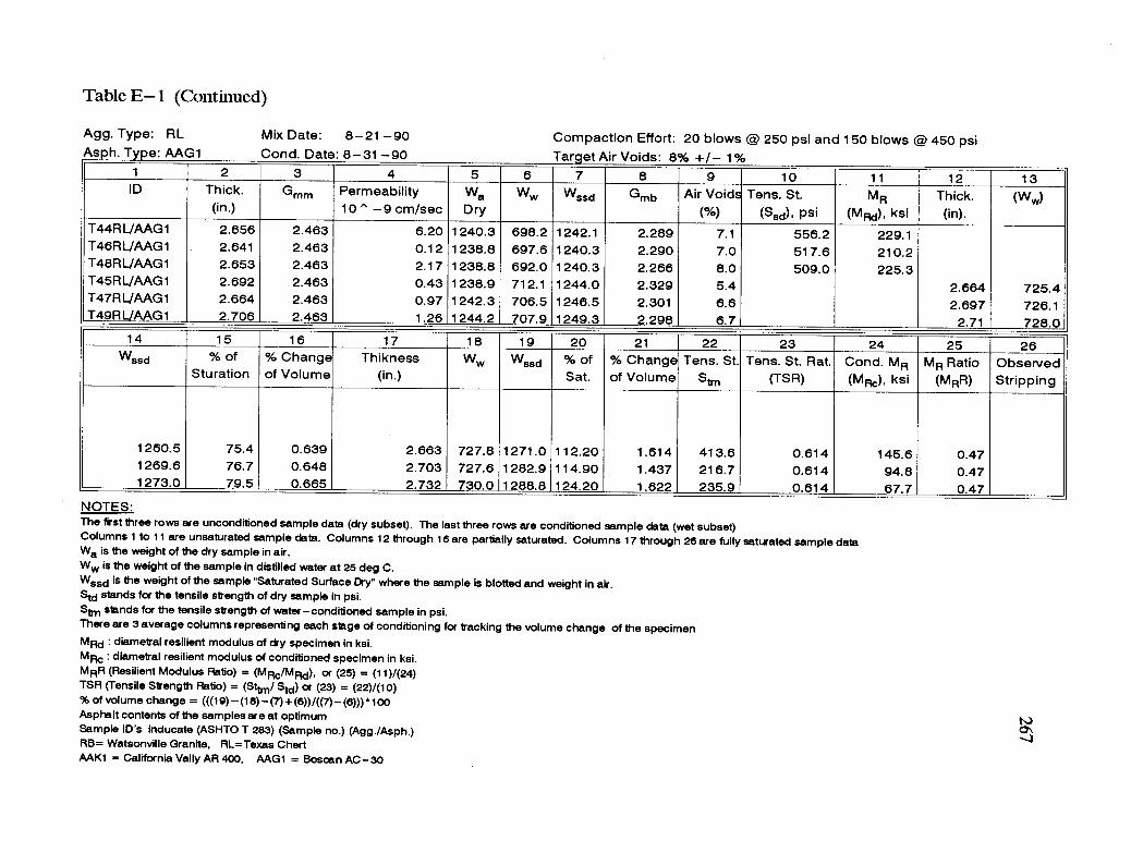
Table E- 1 (Continued)
Agg. Type: RLAs h. T e: AAG1
Mix Date: 8-21-90Cond. Date: 8-31-90
Compaction Effort: 20 blows @ 250 psi and 150 blows @ 450 psiTarget Air Voids: 8% +/- 1%
1 2 3 4 5 6 7 8 9 10 11 12 13ID Thick. Gmm Permeability Wa Ww Wssd Gmb Air Voids Tens. St. MR Thick. (Ww)
(in.) 10 '' -9 cm/sec Dry (%) (Ssd), psi (MRd), ksi (in).T44RL/AAG1 2.656 2.463 6.20 1240.3 698.2 1242.1 2.289 7.1 556.2 229.1T46RL/AAG1 2.641 2.463 0.12 1238.8 697.6 1240.3 2.290 7.0 517.6 210.2T48RL/AAG1 2.653 2.463 2.17 1238.8 692.0 1240.3 2.266 8.0 509.0 225.3T45RL/AAG1 2.692 2.463 0.43 1238.9 712.1 1244.0 2.329 5.4 2.664 725.4T47RL/AAG1 2.664 2.463 0.97 1242.3 706.5 1246.5 2.301 6.6 2.697 726.1T49RL/AAG1 2.706 2.463 1.26 1244.2 707.9 1249.3 2.298 6.7 2.71 728.0
14 15 16 17 18 19 20 21 22 23 24 25 26Wssd % of % Change Thikness Ww Wssd % of % Change Tens. St. Tens. St. Rat. Cond. MR MR Ratio Observed
Sturation of Volume (in.) Sat. of Volume St, (TSR) (MR,), ksi (MRR) Stripping
1260.5 75.4 0.639 2.663 727.8 1271.0 112.20 1.614 413.6 0.614 145.6 0.471269.6 76.7 0.648 2.703 727.6 1282.9 114.90 1.437 216.7 0.614 94.8 0.471273.0 79.5 0.665 2.732 730.0 1288.8 124.20 1.622 235.9_ 0.614 67.7 0.47
NOTES:The first three rows are unconditioned sample data (dry subset). The last three rows are conditioned sample data (wet subset)Columns 1 to 11 are unsaturated sample data. Columns 12 through 16 are partially saturated. Columns17 through 28 are fully saturated sample dataWa is the weight of the dry sample in air.Ww is the weight of the sample in distilled water at 25 deg C.Wssd is the weight of the sample "Saturated Surface Dry where the sample is blotted and weight in air.Std stands for the tensile strength of dry sample in psi.St,., stands for the tensile strength of water-conditioned sample in psi.There are 3 average columns representing each stage of conditioning for tracking the volume change of the specimenMRd : diametral resilient modulus of dry specimen in ksi.MRe : diametral resilient modulus of conditioned specimen in ksi.MRR (Resilient Modulus Ratio) = (MRb/MRd), or (25) = (11)/(24)TSR (Tensile Strength Ratio) = (Sttm/ Std) or (23) = (22)/(10)% of volume change = (((19)- (18)- (7)+(6))/((7)- (6)))*100Asphalt contents of the samples are at optimumSample ID's inducate (ASHTO T 283) (Sample no.) (Agg./Asph.)RB= Watsonville Granite, RL=Texas ChertAAK1 = California Vally AR 400, AAG1 = Boscan AC-30

Table E- 1 (Continued)
Agg. Type: RLAs h. T e: AAK1
Mix Date: 8-23-90Cond. Date: 8-25-90
Compaction Effort: 20 blows @ 250 psi and 150 blows g 450 psiTarget Air Voids: 8% +/- 1%
1 2 3 4 5 6 7 8 9 10 11 12 13ID Thick. Gmm Permeability Wa Ww Wssd Gmb Air Voids Tens. St. MR Thick. (Ww)
(in.) 10 " -9 cm/sec Dry (%) (Ssd), psi (MRd), ksi (in).T51RL/AAK1 2.666 2.455 12.83 1239.7 690.1 1241.7 2.257 8.1 415.1 208.2T54RL/AAK1 2.675 2.455 4.25 1241.4 701.0 1243.1 2.298 6.4 569.8T55RL/AAK1 2.626 2.455 3.59 1239.0 696.6 1241.7 2.283 7.0 520.4 241.1T52RL/AAK1 2.668 2.455 13.85 1238.8 703.9 1242.8 2.299 6.4 2.63 694.9T53RL/AAK1 2.696 2.455 9.53 1240.3 703.3 1243.3 2.297 6.4 2.68 721.1T56RL/AAK1 2.693 2.455 1.27 1244.6 708.3 1247.2 2.310 5.9 2.69 728.0
14 15 16 17 18 19 20 21 22 23 24 25 26Wssd % of % Change Thikness Ww Wssd % of % Change Tens. St. Tens. St. Rat. Cond. MR MR Ratio Observed
Sturation of Volume (in.) Sat. of Volume Stm (TSR) (MR,), ksi (MRR) Stripping
1260.5 63.3 4.955 2.633 728.0 1278.2 115.70 5.739 370.8 0.600 104.0 0.821266.2 74.5 0.944 2.681 730.6 1285.6 131.00 1.508 282.8 0.600 85.6 0.821267.8 72.6 0.167 2.725 732.0 1285.1 127.40 0.653 385.7 0.600 105.7 0.82
NOTES:The first three rows are unconditioned sample data (dry subset). The last three rows are conditioned sample data (wet subset)Columns 1 to 11 are unsaturated sample data. Columns 12 through 18 are partially saturated. Columns 17 through 26 are fully saturated sample dataWa is the weight of the dry sample in air.Ww is the weight of the sample in distilled water at 25 deg C.Wssd is the weight of the sample "Saturated Surface Dry" where the sample is blotted and weight in air.Std stands for the tensile strength of dry sample in psi.Stm stands for the tensile strength of water-conditioned sample in psi.There are 3 average columns representing each stage of conditioning for tracking the volume change of the specimenMRd : diametral resilient modulus of dry specimen in ksi.MRa : diametral resilient modulus of conditioned specimen in ksi.MRR (Resilient Modulus Ratio) = (MRa/MRd), or (25) = (11)/(24)TSR (Tensile Strength Ratio) = (Sttm/ Std) or (23) = (22)/(10)% of volume change = (01 9)- (18)- (7)+(8))/((7)- (8)))*100Asphalt contents of the samples are at optimumSample ID's inducate (ASHTO T 283) (Sample no.) (Agg./Asph.)RB= Watsonville Granite, RL=Texas ChartAAK1 = California Vally AR 400, AAG1 = Boscan AC-30
N00

Table E- 1 (Continued)
Agg. Type: RLAs h. T e: AAK1
Mix Date: 8-27-90Cond. Date: 8-30-90
Compaction Effort: 20 blows @ 250 psi and 150 blows @ 450 psiTarget Air Voids: 8% +/- 1%
1 2 3 4 5 6 7 8 9 10 11 12 13ID Thick. Gmm Permeability Wa We,, Wssd Gmb Air Voids Tens. St. MR Thick. (Ww)
(in.) 10 ^ -9 cm/sec Dry (%) (Ssd), psi (MRd), ksi (in).T61RL/AAK1 2.697 2.447 2.46 1240.7 695.0 1242.1 2.274 7.1 368.0 155.6T62RL/AAK1 2.721 2.447 0.87 1244.7 697.9 1245.5 2.277 7.0 369.6 167.4T63RL/AAK1 2.683 2.447 7.40 1245.7 692.5 1247.0 2.252 8.0 363.8 165.1T58RL/AAK1 2.710 2.447 2.99 1243.3 707.7 1249.6 2.294 6.2 2.70 726.0T59RL/AAK1 2.684 2.447 4.56 1243.5 707.0 1248.4 2.297 6.1 2.71 726.0T6ORL/AAK1 2.687 2.447 1.74 1240.8 704.6 1243.6 2.302 5.9 2.70 724.5
14 15 16 17 18 19 20 21 22 23 24 25 26Wssd % of % Change Thikness Ww Wssd % of % Change Tens. St. Tens. St. Rat. Cond. MR MR Ratio Observed
Sturation of Volume (in.) Sat. of Volume Stm (TSR) (MR,), ksi (MRR) Stripping
1267.2 70.7 -0.129 2.701 728.2 1280.9 112.50 1.046 310.8 0.825 104.7 0.621267.2 71.3 -0.037 2.707 728.0 1278.4 106.00 0.876 294.5 0.825 98.6 0.621263.6 71.4 0.019 2.692 727.3 1275.3 108.60 0.541 276.9 0.825 105.7 0.62
NOTES:The first three rows are unconditioned sample data (dry subset). The last three rows are conditioned sample data (wet subset)Columns 1 to 11 are unsaturated sample data. Columns 12 through 16 are partially saturated. Columns 17 through 26are fully saturated sample dataWa is the weight of the dry sample in air.Ww is the weight of the sample in distilled water at 25 deg C.Wssd is the weight of the sample "Saturated Surface Dry" where the sample is blotted and weight in air.Std stands for the tensile strength of dry sample in psi.San stands for the tensile strength of water-conditioned sample in psi.There are 3 average columns representing each stage of conditioning for tracking the volume change of the specimenMRd : diametral resilient modulus of dry specimen in ksi.MRa : diametral resilient modulus of conditioned specimen in ksi.MRR (Resilient Modulus Ratio) = (MRa/MRd), or (25) = (11)1(24)TSR (Tensile Strength Ratio) = (Stan/ Std) or (23) = (22)/(10)% of volume change = (((19) - (18)- (7)+(6))/((7)-(8)))*100Asphalt contents of the samples are at optimumSample ID's inducate (ASHTO T 283) (Sample no.) (Agg./Asph.)RB= Watsonville Granite, RL=Texas ChertAAK1 = California Vally AR 400, AAG1 = Boscan AC-30

Table E- 1 (Continued)
Agg. Type: RLAs h. Type: AAK1
Mix Date: 9-3-90Cond. Date: 9-5-90
Compaction Effort: 20 blows @ 250 psi and 150 blows @ 450 psiTarget Air Voids: 8% +/- 1%
1 2 3 4 5 6 7 8 9 10 11 12 13ID Thick. Gmm Permeability Wa Ww Wssd Gmb Air Voids Tens. St. MR Thick. (Ww)
(in.) 10 " -9 cm/sec Dry (%) (Ssd), psi (MRd), ksi (in).T68RL/AAK1 2.659 2.449 1.86 1245.3 700.7 1246.5 2.287 6.6 330.5 168.6T69RL/AAK1 2.673 2.449 14.50 1242.0 693.9 1243.5 2.267 7.4 375.0 159.1T7ORL/AAK1 2.690 2.449 4.21 1245.4 700.2 1246.5 2.285 6.7 411.4 153.4T65RL/AAK1 2.668 2.449 1.75 1230.6 700.4 1233.7 2.308 5.8 2.65 720.0T66RL/AAK1 2.675 2.449 1.89 1239.9 705.9 1242.9 2.309 5.7 2.67 725.4T67R1../AAK1 2.665 2.449 5.71 1240.0 705.7 1242.5 2.310 5.7 2.67 726.0
14 15 16 17 18 19 20 21 22 23 24 25 26Wssd % of % Change Thikness Ww Wssd % of % Change Tens. St. Tens. St. Rat. Cond. MR MR Ratio Observed
Sturation of Volume (in.) Sat. of Volume Stm (TSR) (MRc), ksi (MRIR) Stripping
1253.8 75.3 0.094 2.670 724.4 1268.2 122.80 0.679 223.1 0.530 79.3 0.531262.6 73.9 0.037 2.683 729.5 1279.1 128.40 0.599 194.1 0.530 82.2 0.531263.2 76.1 0.075 2.676 730.5 1278.7 127.60 0.543 216.5 0.530 86.4 0.53
NOTES:The first three rows are unconditioned sample data (dry subset). The last three rows are conditioned sample data (wet subset)Columns 1 to 11 are unsaturated sample data. Columns 12 through 16 are partially saturated. Columns17 through 26 are fully saturated sample dataWa is the weight of the dry sample in air.Ww is the weight of the sample in distilled water at 25 deg C.Wssd is the weight of the sample "Saturated Surface Dry" where the sample is blotted and weight in air.Std stands for the tensile strength of dry sample in psi.Stm stands for the tensile strength of water-conditioned sample in psi.There are 3 average columns representing each stage of conditioning for tracking the volume change of the specimenMRd : diametral resilient modulus of dry specimen in ksi.MRb : diametral resilient modulus of conditioned specimen in ksi.MRR (Resilient Modulus Ratio) = (MRe/MRd), or (25) = (11)/(24)TSR (Tensile Strength Ratio) = (Stan/ Std) or (23) = (22)/(10)% of volume change = (((19) - (18) (7) + (6))/((7) - (6)))*100Asphalt contents of the samples are at optimumSample ID's inducate (ASHTO T 283) (Sample no.) (Agg./Asph.)R8= Watsonville Granite, RL=Texas ChartAAK1 = California Vally AR 400, AAG1 = Boscan AC-30
t.)O
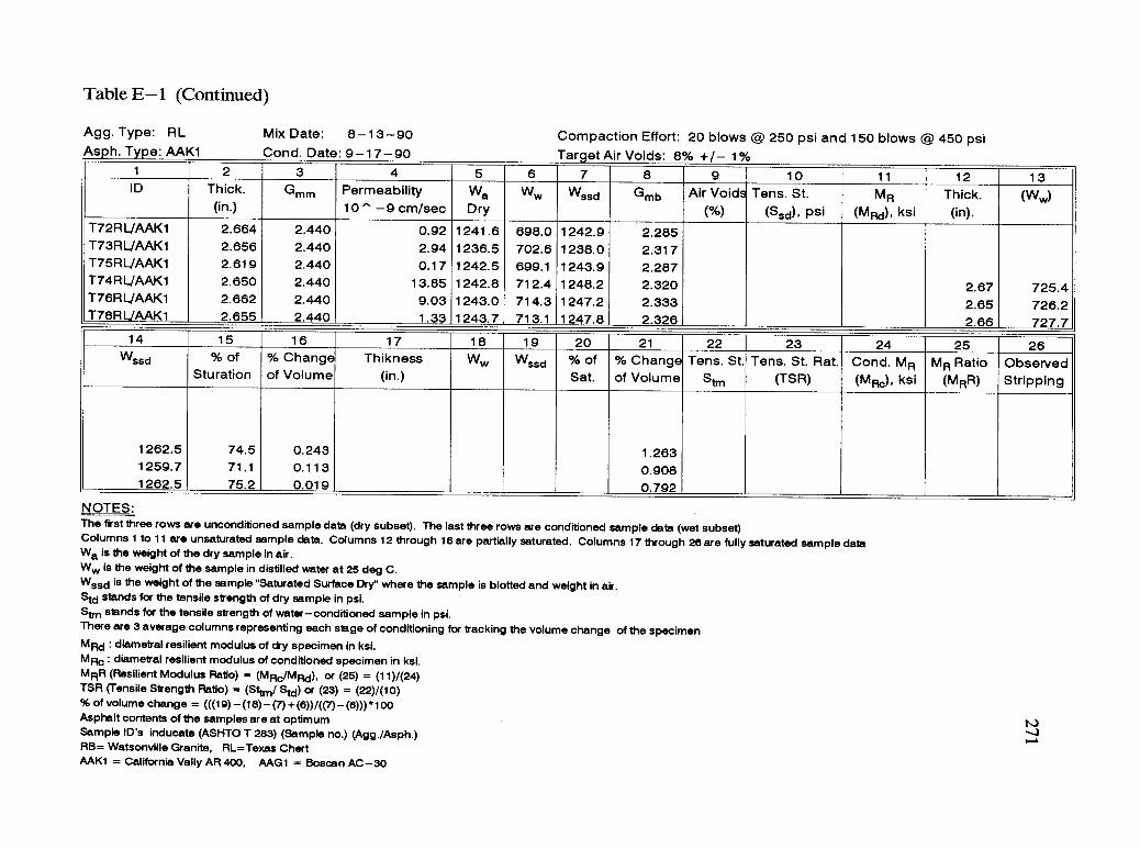
Table E- 1 (Continued)
Agg. Type: RLAs h. T e: AAK1
Mix Date: 8-13-90Cond. Date: 9-17-90
Compaction Effort: 20 blows @ 250 psi and 150 blows @ 450 psiTarget Air Voids: 8% +/- 1%
1 2 3 4 5 6 7 8 9 10 11 12 13ID Thick. Gmm Permeability Wa Ww Wssd Gmb Air Voids Tens. St. MR Thick. (Ww)
(in.) 10 ^ -9 cm/sec Dry (%) (Ssd), psi (MR,d), ksi (in).T72RL/AAK1 2.664 2.440 0.92 1241.6 698.0 1242.9 2.285T73RL/AAK1 2.656 2.440 2.94 1236.5 702.6 1238.0 2.317T75RL/AAK1 2.619 2.440 0.17 1242.5 699.1 1243.9 2.287T74RL/AAK1 2.650 2.440 13.85 1242.8 712.4 1248.2 2.320 2.67 725.4T76R1./AAK1 2.662 2.440 9.03 1243.0 714.3 1247.2 2.333 2.65 726.2T78RLJAAK1 2.655 2.440 1.33 1243.7 713.1 1247.8 2.326 2.66 727.7
14 15 16 17 18 19 20 21 22 23 24 25 26Wssd % of % Change Thikness Ww Wssd % of % Change Tens. St. Tens. St. Rat. Cond. MR MR Ratio Observed
Sturation of Volume (in.) Sat. of Volume S" (TSR) (MR,), ksi (MRR) Stripping
1262.5 74.5 0.243 1.2631259.7 71.1 0.113 0.9081262.5 75.2 0.019 0.792
NOTES:The first three rows are unconditioned sample data (dry subset). The last three rows are conditioned sample data (wet subset)Columns 1 to 11 are unsaturated sample data. Columns 12 through 16 are partially saturated. Columns 17 through 26 are fully saturated sample dataWa is the weight of the dry sample in air.Ww is the weight of the sample in distilled water at 25 deg C.Wssd is the weight of the sample "Saturated Surface Dry" where the sample is blotted and weight in air.Std stands for the tensile strength of dry sample in psi.St,, stands for the tensile strength of water-conditioned sample in psi.There are 3 average columns representing each stage of conditioning for tracking the volume change of the specimenMRd : diametral resilient modulus of dry specimen in ksi.MRc : diametral resilient modulus of conditioned specimen in ksi.MRR (Resilient Modulus Ratio) = (MRc/MR1), or (25) = (11)/(24)TSR (Tensile Strength Ratio) = (Sttm/ Std) or (23) --= (22)/(10)% of volume change = (((19) - (18)- (7)+(6))/((7)-(6)))*100Asphalt contents of the samples are at optimumSample ID's inducate (ASHTO T 283) (Sample no.) (Agg./Asph.)RB= Watsonville Granite, RL=Texas ChertAAK1 = California Vally AR 400, AAG1 = Boscan AC-30
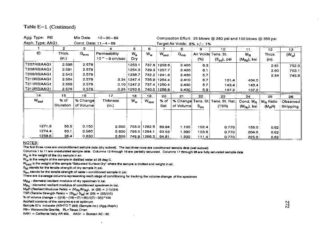
Table E- 1 (Continued)
Agg. Type: RBAs h. T e: AAG1
Mix Date: 10-30-89Cond. Date: 11-4-89
Compaction Effort: 25 blows @ 250 psi and 150 blows @ 350 psiTarget Air Voids: 8% +/- 1%
1 2 3 4 5 6 7 8 9 10 11 12 13ID Thick. Gmm Permeability Wa Ww Wssd Gmb Air Voids Tens. St. MR Thick. (Ww)
(in.) 10 ^ -9 cm/sec Dry (%) (Ssd), psi (MRd), ksi (in).T207RB/AAG1 2.598 2.578 1253.1 737.8 1256.6 2.420 6.3 2.61 752.0T208RB/AAG1 2.591 2.578 1254.3 739.3 1257.7 2.420 6.1 2.60 753.1T209RB/AAG1 2.543 2.578 1238.7 732.2 1241.8 2.430 5.7 2.54 745.8T21ORB/AAG1 2.584 2.578 3.34 1247.4 735,9 1254.4 2.410 6.7 131.4 404.0T211RB/AAG1 2.568 2.578 0.10 1247.2 737.4 1250.4 2.430 5.7 143.4 143.4T212RB/AAG1 2.578 2.578 0.25 1253.8 740.0 1256.8 2.430 5.9 137.2 137.2
14 15 16 17 18 19 20 21 22 23 24 25 26Wssd % of % Change Thikness Ww Wssd % of % Change Tens. St. Tens. St. Rat. Cond. MR MR Ratio Observed
Sturation of Volume (in.) Sat. of Volume Strn (TSR) (MRd), ksi (MRR) Stripping
1271.6 56.5 0.150 2.600 758.0 1282.5 89.84 1.100 102.4 0.770 158.0 0.621274.4 63.1 0.560 2.600 758.5 1284.1 93.53 1.390 103.8 0.770 204.0 0.621258.6 38.4 0.630 2.600 749.9 1266.3 94.81 1.330 111.4 0.770 225.0 0.62
NOTES:The first three rows are unconditioned sample data (dry subset). The last three rows are conditioned sample data (wet subset)Columns 1 to 11 are unsaturated sample data. Columns 12 through 16 are partially saturated. Columns 17 through 26are fully saturated sample dataWa is the weight of the dry sample in air.W, is the weight of the sample in distilled water at 25 deg C.Wssd is the weight of the sample "Saturated Surface Dry" where the sample is blotted and weight in air.Std stands for the tensile strength of dry sample in psi.Stm stands for the tensile strength of water-conditioned sample in psi.There are 3 average columns representing each stage of conditioning for tracking the volume change of the specimenMRd : diametral resilient modulus of dry specimen in ksi.MRb : diametral resilient modulus of conditioned specimen in ksi.MRR (Resilient Modulus Ratio) = (MRc/MRd), or (25) = (11)/(24)TSR (Tensile Strength Ratio) = (Sttm/ Std) or (23) = (22)/(10)% of volume change = (((19)- (18)- (7)+(6))/((7)- (6)))*100Asphalt contents of the samples are at optimumSample ID's inducate (ASHTO T 283) (Sample no.) (Agg./Asph.)RI3= Watsonville Granite, RL=Texas ChartAAK1 = California Vally AR 400, AAG1 = Boscan AC-30
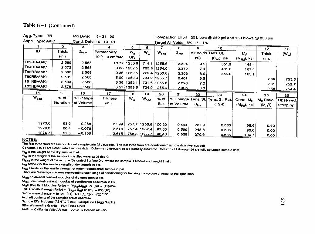
Table E- 1 (Continued)
Agg. Type: RBAs h. T e: AAK1
Mix Date: 9-21-90Cond. Date: 10-10-91
Compaction Effort: 20 blows @ 250 psi and 150 blows @ 250 psiTarget Air Voids: 8% +/- 1%
1 2 3 4 5 6 7 8 9 10 11 12 13ID Thick. Gmm Permeability Wa Ww Wssd Gmb Air Voids Tens. St. MR Thick. (Ww)(in.) 10 's -9 cm/sec Dry (%) (Ssd), psi (M Rd), ksi (in).
T82RB /AAK1 2.589 2.568 18.77 1253.8 714.1 1255.6 2.324 9.5 351.9 148.4T84RB/AAK1 2.572 2.568 0.33 1252.5 725.8 1254.0 2.379 7.4 401.8 167.4T85RB /AAK1 2.586 2.568 0.36 1252.5 722.4 1253.6 2.363 8.0 365.0 165.1T8ORB/AAK1 2.601 2.568 5.00 1252.0 734.2 1255.7 2.401 6.5 2.59 753.5T81RB/AAK1 2.633 2.568 5.39 1252.1 731.6 1255.6 2.390 7.0 2.61 752.7T83RB /AAK1 2.578 2.568 0.51 1253.5 734.9 1255.9 2.406 6.3 2.58 754.4
14 15 16 17 18 19 20 21 22 23 24 25 26Wssd % of % Change Thikness Ww Wssd % of % Change Tens. St. Tens. St. Rat. Cond. MR MR Ratio Observed
Sturation of Volume (in.) Sat. of Volume Stm (TSR) (MR,), ksi (MRR) Stripping
1273.6 63.6 -0.268 2.599 757.7 1285.8 100.20 0.444 237.9 0.635 98.6 0.601276.3 66.4 -0.076 2.616 757.4 1287.4 97.60 0.596 248.8 0.635 96.6 0.601274.7 61.5 -0.136 2.615 758.3 1285.7 98.40 0.328 270.6 0.635 104.7 0.60
NOTES:The first three rows are unconditioned sample data (dry subset). The lastthree rows are conditioned sample data (wet subset)Columns 1 to 11 are unsaturated sample data. Columns 12 through 18 are partially saturated. Columns 17 through 28 are fully saturated sample dataWa is the weight of the dry sample in air.Ww is the weight of the sample in distilled water at 25 deg C.Wssd is the weight of the sample "Saturated Surface Dry" where the sample is blotted and weight in air.Std stands for the tensile strength of dry sample in psi.Stm stands for the tensile strength of water-conditioned sample in psi.There are 3 average columns representing each stage of conditioning for tracking the volume change of the specimenMRd : diametral resilient modulus of dry specimen in ksi.MRc : diametral resilient modulus of conditioned specimen in ksi.MRR (Resilient Modulus Ratio) = (MRc/MRd), or (25) = (11)1(24)TSR (Tensile Strength Ratio) = (Sttm/ Std) or (23) = (22)/(10)% of volume change = (((19) (18)- (7)+ (6))/((7)- (6)))*100Asphalt contents of the samples are at optimumSample ID's inducate (ASHTO T 283) (Sample no.) (AggiAsph.)RB= Watsonville Granite, RL=Texas ChertAAK1 = California Vally AR 400, AAG1 = Boscan AC-30

Table E- 1 (Continued)
Agg. Type: RBAs h. T e: AAK1
Mix Date: 7-5-90Cond. Date: 10-12-90
Compaction Effort: 20 blows @ 250 psi and 150 blows @ 250 psiTarget Air Voids: 8% +/- 1%
1 2 3 4 5 6 7 8 9 10 11 12 13ID Thick. Gmm Permeability Wa Ww Wssd Gmb Air Voids Tens. St. MR Thick. (Ww)(in.) 10 " -9 cm/sec Dry (%) (Sad). psi (MRd), ksi (in).
T89RB/AAK1 2.671 2.550 31.23 1258.2 712.1 1258.0 2.304 9.7 396.0 139.9T90RB/AAK1 2.566 2.550 1.37 1252.8 724.5 1253.6 2.372 6.2 380.4 174.7T91RB/AAK1 2.584 2.550 0.00 1255.3 732.7 1256.1 2.402 5.0 462.8 183.1T87RB/AAK1 2.636 2.550 5.75 1257.7 738.2 1266.2 2.382 6.6 2.67 754.2T88RB/AAK1 2.686 2.550 15.26 1255.1 734.7 1263.2 2.375 6.9 2.64 751.5T92RB/AAK1 2.587 2.550 0.02 1254.8 740.1 1258.5 2.421 4.3 2.59 753.8
14 15 16 17 18 19 20 21 22 23 24 25 26Wssd % of % Change Thikness Ww Wssd % of % Change Tens. St. Tens. St. Rat. Cond. MR MR Ratio Observed
Sturation of Volume (in.) Sat. of Volume Stm (TSR) (Mild, ksi (MRR) Stripping
1281.1 67.3 -0.208 2.675 759.4 1291.7 99.30 1.424 285.9 0.646 106.4 0.611279.5 67.2 -0.095 2.644 757.1 1290.5 99.00 1.460 258.5 0.646 92.8 0.611271.2 73.8 -0.193 2.625 758.4 1283.0 127.70 0.525 365.8 0.646 130.1 0.61
NOTES:The first three rows are unconditioned sample data (dry subset). The last three rows are conditioned sample data (wet subset)Columns 1 to 11 are unsaturated sample data. Columns 12 through 16 are partially saturated. Columns 17 through 26 are fully saturated sample dataWa is the weight of the dry sample in air.Ww is the weight of the sample in distilled water at 25 deg C.Wssd is the weight of the sample "Saturated Surface Dry where the sample is blotted and weight in air.Std stands for the tensile strength of dry sample in psi.Stm stands for the tensile strength of water-conditioned sample in psi.There are 3 average columns representing each stage of conditioning for tracking the volume change of the specimenMRd : diametral resilient modulus of dry specimen in ksi.MRe : diametral resilient modulus of conditioned specimen in ksi.MRR (Resilient Modulus Ratio) = (MRc/MRd), or (25) = (11)/(24)TSR (Tensile Strength Ratio) = (Sttm/ Std) or (23) = (22)/(10)% of volume change = (((19)- (18)- (7)+(6))/((7)- (6)))*100Asphalt contents of the samples are at optimumSample ID's inducate (ASHTO T 283) (Sample no.) (Agg./Asph.)RB= Watsonville Granite, RL=Texas ChertAAK1 = California Valty AR 400, AAG1 = Boscan AC-30

Table E- 1 (Continued)
Agg. Type: RBAs h. Type: AAG1
Mix Date: 9-4-90Cond. Date: 9-10-90
Compaction Effort: 20 blows @ 250 psi and 150 blows @ 450 psiTarget Air Voids: 8% +/- 1%
1 2 3 4 5 6 7 8 9 10 11 12 13ID Thick. Gmm Permeability Wa Ww Wssd Gmb Air Voids Tens. St. MR Thick. (Ww)(in.) 10 ^ -9 cm/sec Dry (%) (S8c1), psi (MRd), ksi (in).
T93RB/AAG1 2.558 2.570 2.40 1248.4 728.1 1249.1 2.400 6.6 477.2 261.5T94RB/AAG1 2.518 2.570 3.29 1249.9 726.2 1251.5 2.387 7.1 478.2 241.6T95RB/AAG1 2.566 2.570 0.00 1249.8 735.4 1251.1 2.430 5.4 526.2 269.0T96RB/AAG1 2.555 2.570 0.08 1253.5 742.2 1258.2 2.429 5.5 2.56 757.8T97RB/AAG1 2.257 2.570 1.44 1248.6 741.4 1253.0 2.441 5.0 2.56 758.0T98RB/AAG1 2.531 2.570 0.00 1253.2 744.2 1255.6 2.451 4.6 2.54 760.1
14 15 16 17 18 19 20 21 22 23 24 25 26Wssd % of % Change Thikness Ww Wssd % of % Change Tens. St. Tens. St. Rat. Cond. MR MR Ratio Observed
Sturation of Volume (in.) Sat. of Volume Stm (TSR) (MRe), ksi (MRR) Stripping
1274.6 74.7 0.155 2.563 759.1 1280.9 97.90 1.076 660.4 1.240 136.1 0.621269.8 82.3 0.039 2.559 759.1 1275.1 103.80 0.907 585.0 1.240 171.0 0.621273.1 83.7 0.313 2.540 762.1 1279.9 112.80 0.786 666.2 1.240 166.7 0.62
NOTES:The first three rows are unconditioned sample data (dry subset). The lastthree rows are conditioned sample data (wet subset)Columns 1 to 11 are unsaturated sample data. Columns 12 through 18are partially saturated. Columns 17 through 28 are fully saturated sample dataWa is the weight of the dry sample in air.Ww is the weight of the sample in distilled water at 25 deg C.Wssd is the weight of the sample "Saturated Surface Dry" where the sample is blotted and weight in air.Std stands for the tensile strength of dry sample in psi.Stm stands for the tensile strength of water-conditioned sample in psi.There are 3 average columns representing each stage of conditioning for tracking the volume change of the specimenMRd : diametral resilient modulus of dry specimen in ksi.MRb : diametral resilient modulus of conditioned specimen in ksi.MRR (Resilient Modulus Ratio) = (MRc/MRd), or (25) = (11)/(24)TSR (Tensile Strength Ratio) = (Sttm/ Std) or (23) = (22)/(10)% of volume change = (((19) - (18)- (7)+(8))/((7)-(8)))*100Asphalt contents of the samples are at optimumSample ID's inducate (ASHTO T 283) (Sample no.) (Agg./Asph.)RB= Watsonville Granite, RL=Texas ChertAAK1 = California Vally AR 400, AAG1 = Boscan AC-30

Table E- 1 (Continued)
Agg. Type: RBAs h. T e: AAK1
Mix Date: 7-31-90Cond. Date: 10-29-90
Compaction Effort: 20 blows @ 200 psi and 150 blows @ 200 psiTarget Air Voids: 8% +/- 1%
1 2 3 4 5 6 7 8 9 10 11 12 13ID Thick. G Permeability Wa Ww Wssd Gmb Air Voids Tens. St. MR Thick. (Ww)
(in.) 10 ^ -9 cm/sec Dry (%) (Ssd). psi (MRd), ksi (in).T99R6/AAK1 2.616 2.606 0.66 1251.6 722.1 1251.8 2.364 9.3 388.8 157.8T100RB/AAK1 2.629 2.606 6.36 1252.3 721.8 1252.8 2.360 9.4 411.7 178.0T101RB/AAK1 2.604 2.606 19.53 1255.7 720.2 1256.2 2.345 10.0 421.8 168.1T102RB/AAK1 2.616 2.606 2.88 1259.2 742.3 1265.0 2.409 7.6 2.56 758.47103R B/AAK1 2.600 2.606 4.99 1251.8 735.2 1258.0 2.394 8.1 2.56 752.6T104RB/AAK1 2.611 2.606 1.79 1253.9 736.2 1259.2 2.398 8.0 2.54 754.7
14 15 16 17 18 19 20 21 22 23 24 25 26Wssd % of % Change Thikness Ww Wssd % of % Change Tens. St. Tens. St. Rat. Cond. MR MR Ratio Observed
Sturation of Volume (in.) Sat. of Volume Stm (TSR) (MRc), ksi (MRR) Stripping
1280.7 54.4 -0.077 2.624 762.9 1287.9 73.50 1.045 353.5 0.811 122.0 0.621275.0 54.7 -0.077 2.626 756.4 1283.0 74.40 1.123 322.2 0.811 115.2 0.621276.7 54.5 -0.191 2.617 759.0 1284.9 74.80 0.831 373.1 0.811 134.6 0.62
NOTES:The first three rows are unconditioned sample data (dry subset). The last three rows are conditioned sample data (wet subset)Columns 1 to 11 are unsaturated sample data. Columns 12 through 16 are partially saturated. Columns 17 through 26 are fully saturated sample dataWa is the weight of the dry sample in air.Ww is the weight of the sample in distilled water at 25 deg C.Wssd is the weight of the sample "Saturated Surface Dry" where the sample is blotted and weight in air.Std stands for the tensile strength of dry sample in psi.Stm stands for the tensile strength of water-conditioned sample in psi.There are 3 average columns representing each stage of conditioning for tracking the volume change of the specimenMRd : diametral resilient modulus of dry specimen in ksi.MRa : diametral resilient modulus of conditioned specimen in ksi.MRR (Resilient Modulus Ratio) = (MRb/MRd), or (25) = (11)/(24)TSR (Tensile Strength Ratio) = (Sttm/ Std) or (23) = (22)/(10)% of volume change = (((19) (18)- (7)+ (6))/((7)- (8)))*100Asphalt contents of the samples are at optimumSample ID's inducate (ASHTO T 283) (Sample no.) (Agg./Asph.)RB= Watsonville Granite, RL=Texas ChertAAK1 = California Vally AR 400, AAG1 = Boscan AC-30

Table E- 1 (Continued)
Agg. Type: RIB.
As h. Type: AAG1Mix Date: 10-10-90Cond. Date: 10 -17 -90
Compaction Effort: 20 blows @ 200 psi and 150 blows @ 200 psiTarget Air Voids: 8% +1- 1%
1 2 3 4 5 6 7 8 9 10 11 12 13ID Thick. G Permeability Wa Ww Wssd Gmb Air Voids Tens. St. MR Thick. (Ww)
(in.) 10 ^ -9 cm/sec Dry (%) (Ssd), psi (MRd), ksi (in).T11ORB/AAG1 2.592 2.570 3.74 1250.3 721.5 1251.9 2.365 8.0 434.5 225.1T112RB/AAG1 2.575 2.570 2.88 1251.1 721.2 1252.1 2.362 8.1 505.6 222.5T114RB/AAG1 2.535 2.570 1.71 1252.2 726.8 1253.1 2.384 7.2 520.0 231.6T109RB/AAG1 2.542 2.570 1.33 1247.1 733.2 1249.9 2.414 6.1 2.59 751.3T111RB/AAG1 2.594 2.570 0.00 1249.3 738.9 1251.3 2.438 5.1 2.54 753.2T113RB/AAG1 2.615 2.570 4.09 1255.5 739.2 1261.6 2.403 6.5 2.61 754.8
14 15 16 17 18 19 20 21 22 23 24 25 26Wssd % of % Change Thikness Ww Wssd % of % Change Tens. St. Tens. St. Rat. Cond. MR MR Ratio Observed
Sturation of Volume (in.) Sat. of Volume Stm (TSR) (Mild, ksi (MRR) Stripping
1266.9 63.0 -0.213 2.593 755.4 1277.3 96.60 0.331 537.1 1.161 186.6 0.831264.7 58.6 -0.176 2.593 756.2 1272.6 89.00 0.216 653.8 1.161 233.3 0.831276.4 61.7 -0.153 2.613 757.8 1285.5 89.60 1.027 523.1 1.161 147,0 0.83
NOTES:The first three rows are unconditioned sample data (dry subset). The last three rows are conditioned sample data (wet subset)Columns 1 to 11 are unsaturated sample data. Columns 12 through 16 are partially saturated. Columns 17 through 28 are fully saturated sample dataWa is the weight of the dry sample in air.Ww is the weight of the sample in distilled water at 25 deg C.Wssd is the weight of the sample "Saturated Surface Dry" where the sample is blotted and weight in air.Std stands for the tensile strength of dry sample in psi.Stm stands for the tensile strength of water-conditioned sample in psi.There are 3 average columns representing each stage of conditioning for tracking the volume change of the specimenMRd : diametral resilient modulus of dry specimen in ksi.MRc : diametral resilient modulus of conditioned specimen in ksi.MRR (Resilient Modulus Ratio) = (MRc/MRd), or (25) = (11)/(24)TSR (Tensile Strength Ratio) = (Sttm/ Std) or (23) = (22)/(10)% of volume change = (((19)- (18) (7)+(6))/((7) - (6)))*100Asphalt contents of the samples are at optimumSample ID's inducate (ASHTO T 283) (Sample no.) (Agg./Asph.)RB= Watsonville Granite, RL=Texas ChertAAK1 = California Vally AR 400, AAG1 = Boscan AC-30
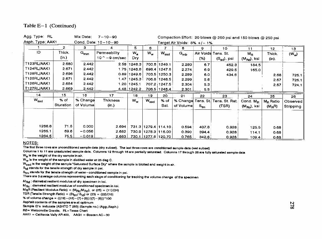
Table E- 1 (Continued)
Agg. Type: RLAs h. T e: AAK1
Mix Date: 7-10-90Cond. Date: 10-10-90
Compaction Effort: 20 blows @ 250 psi and 150 blows @ 250 psiTarget Air Voids: 8% +/- 1%
1 2 3 4 5 6 7 8 9 10 11 12 13ID Thick. Gmm Permeability Wa Ww Wssd Gmb Air Voids Tens. St. MR Thick.
(in.) 10 ^ -9 cm/sec Dry (%) (Sad), psi (MRd), ksi (in).T123RL/AAK1 2.680 2.442 2.58 1248.3 700.6 1249.1 2.280 6.7 452.3 184.5T124RL/AAK1 2.671 2.442 1.75 1246.8 698.4 1247.5 2.274 6.9 429.5 165.0T128RL/AAK1 2.696 2.442 0.89 1249.6 703.5 1250.3 2.289 6.0 434.6 2.68 725.1T125RL/AAK1 2.671 2.442 1.47 1245.3 706.8 1248.5 2.299 5.6 2.67 725.1T126RL/AAK1 2.684 2.442 1.20 1245.1 707.2 1247.5 2.304 5.3 2.67 724.1T127RL/AAK1 2.669 2.442 4.48 1242.2 706.5 1246.4 2.301 5.5
14 15 16 17 18 19 20 21 22 23 24 25 26Wssd % of % Change Thikness Ww Wssd % of % Change Tens. St. Tens. St. Rat. Cond. MR MR Ratio Observed
Sturation of Volume (in.) Sat. of Volume Stm (TSR) (MRc), ksi (MRR) Stripping
1266.8 71.5 0.000 2.694 731.3 1279.4 114.10 0.594 407.8 0.928 125.5 0.681265.1 69.6 -0.056 2.682 730.9 1278.3 116.00 0.390 394.4 0.928 114.1 0.681264.5 75.5 -0.019 2.683 730.1 1277.6 120.70 0.765 342.6 0.928 109.4 0.68
NOTES:The first three rows are unconditioned sample data (dry subset). The last three rows are conditioned sample data (wet subset)Columns 1 to 11 are unsaturated sample data. Columns 12 through 16 are partially saturated. Columns 17 through 26 are fully saturated sample dataWa is the weight of the dry sample in air.Ww is the weight of the sample in distilled water at 25 deg C.Wssd is the weight of the sample "Saturated Surface Dry" where the sample is blotted and weight in air.Std stands for the tensile strength of dry sample in psi.Stm stands for the tensile strength of water-conditioned sample in psi.There are 3 average columns representing each stage of conditioning for tracking the volume change of the specimenMRd : diametral resilient modulus of dry specimen in ksi.MRc : diametral resilient modulus of conditioned specimen in ksi.MRR (Resilient Modulus Ratio) = (MRc/MRd), or (25) = (11)/(24)TSR (Tensile Strength Ratio) = (Stan/ Sid) or (23) = (22)/(10)% of volume change = (((19)- (18)- (7)+(6))/((7)- (6)))*100Asphalt contents of the samples are at optimumSample ID's inducate (ASHTO T 283) (Sample no.) (Agg./Asph.)RB= Watsonville Granite, RL=Texas ChertAAK1 = California Vally AR 400, AAG1 = Boscan AC-30
t.)00
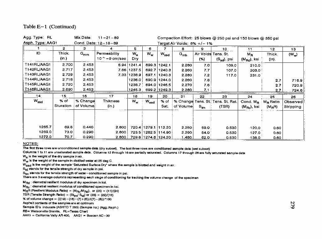
Table E- 1 (Continued)
Agg. Type: RLAs h. T e: AAG1
Mix Date: 11 -21 -89Cond. Date: 12-18-89
Compaction Effort: 25 blows @ 250 psi and 150 blows @ 350 psiTarget Air Voids: 8% +/- 1%
1 2 3 4 5 6 7 8 9 10 11 12 13ID Thick. Gmm Permeability Wa Ww Wssd Gmb Air Voids Tens. St. MR Thick. (Ww)
(in.) 10 ^ -9 cm/sec Dry (%) (Ssd), psi (MRc1). ksi (in).T141RL/AAG1 2.700 2.453 6.94 1241.4 699.3 1242.1 2.280 7.0 109.0 210.0T142RL/AAG1 2.717 2.453 7.66 1237.5 692.7 1240.3 2.260 7.7 107.0 203.0T143RL/AAG1 2,729 2.453 7.33 1238.9 697.1 1240.3 2.280 7.2 117.0 231.0T144RL/AAG1 2.718 2.453 1236.0 690.9 1244.0 2.260 7.8 2.7 716.9T145RLJAAG1 2.720 2.453 1238.7 694.0 1246.5 2.270 7.6 2.7 720.9T146RL/AAG1 2.690 2.453 1245.3 699.2 1249.3 2.280 7.1 2.7 724.6
14 15 16 17 18 19 20 21 22 23 24 25 26Wssd % of % Change Thikness Ww Wssd % of % Change Tens. St. Tens. St. Rat. Cond. MR MR Ratio Observed
Sturation of Volume (in.) Sat. of Volume Stm (TSR) (MR,), ksi (MO) Stripping
1265.7 69.8 0.440 2.800 720.4 1279.1 112.20 2.250 59.0 0.530 120.0 0.601269.0 73.0 0.290 2.800 723.5 1282.5 114.90 2.290 54.0 0.530 127.0 0.601272.0 70.7 0.290 2.800 729.8 1274.6 124.20 1.480 62.0 0.530 138.0 0.60
NOTES:The first three rows are unconditioned sample data (dry subset). The last three rows are conditioned sample data (wet subset)Columns 1 to 11 are unsaturated sample data. Columns 12 through 16 are partially saturated. Columns 17 through 26 are fully saturated sample dataWa is the weight of the dry sample in air.Ww is the weight of the sample in distilled water at 25 deg C.Wssd is the weight of the sample "Saturated Surface Dry" where the sample is blotted and weight in air.Std stands for the tensile strength of dry sample in psi.Stm stands for the tensile strength of water-conditioned sample in psi.There are 3 average columns representing each stage of conditioning for tracking the volume change of the specimen
MRd : diametral resilient modulus of dry specimen in ksi.MRb : diametral resilient modulus of conditioned specimen in ksi.MRR (Resilient Modulus Ratio) = (MRc/MRd), or (25) = (11)/(24)TSR (Tensile Strength Ratio) = (Stan/ Std) or (23) = (22)/(10)% of volume change = (((19)- (18)- (7)+(6))/((7)- (6)))*100Asphalt contents of the samples are at optimumSample ID's inducate (ASHTO T 283) (Sample no.) (Agg./Asph.)RB= Watsonville Granite, RL=Texas ChertAAK1 = California Vally AR 400, AAG1 = Bosaan AC-30
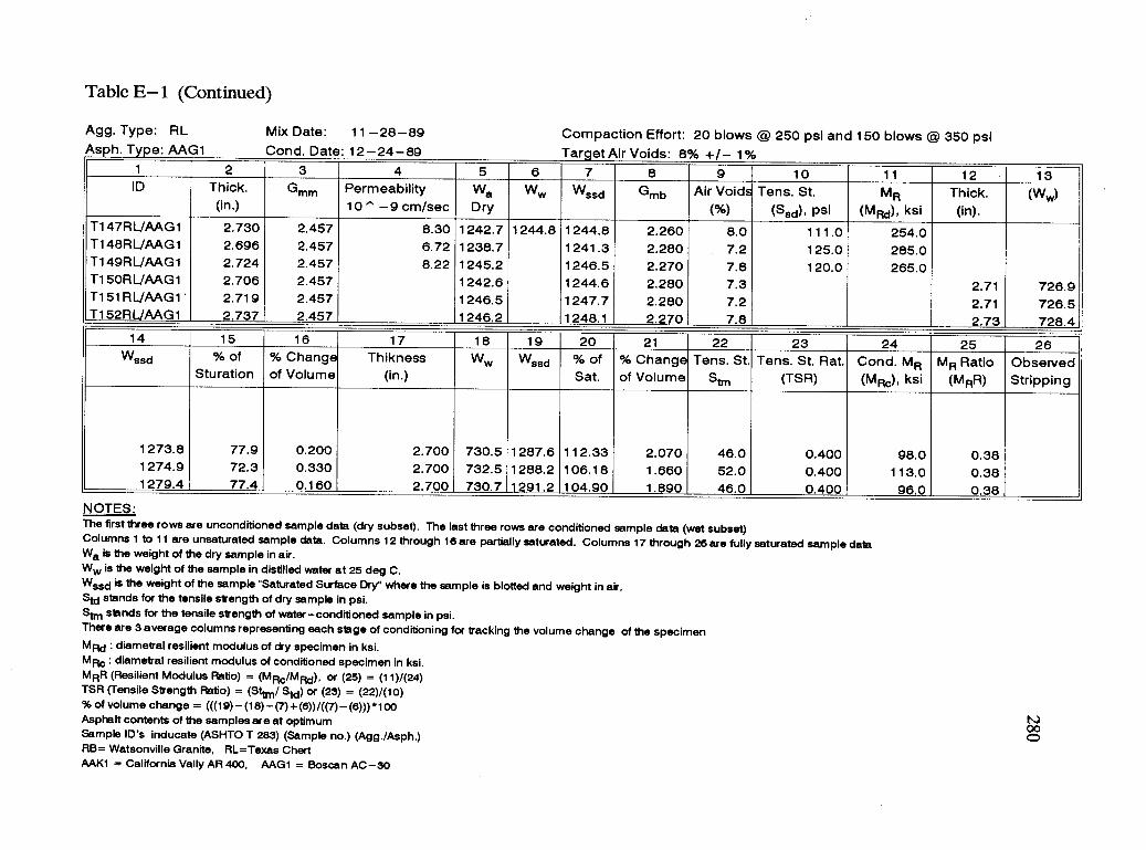
Table E- 1 (Continued)
Agg. Type: RLAs h. T e: AAG1
Mix Date: 11-28-89Cond. Date: 12-24-89
Compaction Effort: 20 blows @ 250 psi and 150 blows @ 350 psiTarget Air Voids: 8% +/- 1%
1 2 3 4 5 6 7 8 9 10 11 12 13ID Thick. Gmm Permeability Wa Ww Wssd Gmb Air Voids Tens. St. MR Thick. (Ww)
(in.) 10 ''` -9 cm/sec Dry (%) (Sad), psi (MRd), ksi (in).T147RL/AAG1 2.730 2.457 8.30 1242.7 1244.8 1244.8 2.260 8.0 111.0 254.0T148RL/AAG1 2.696 2.457 6.72 1238.7 1241.3 2.280 7.2 125.0 285.0T149RI_JAAG1 2.724 2.457 8.22 1245.2 1246.5 2.270 7.8 120.0 265.0T15ORL/AAG1 2.706 2.457 1242.6 1244.6 2.280 7.3 2.71 726.9T151RL/AAG1' 2.719 2.457 1246.5 1247.7 2.280 7.2 2.71 726.5T152RL/AAG1 2.737 2.457 1246.2 1248.1 2.270 7.8 2.73 728.4
14 15 16 17 18 19 20 21 22 23 24 25 26Wssd % of % Change Thikness Ww Wssd % of % Change Tens. St. Tens. St. Rat. Cond. MR MR Ratio Observed
Sturation of Volume (in.) Sat. of Volume Stm (TSR) (Mild), ksi (MRR) Stripping
1273.8 77.9 0.200 2.700 730.5 1287.6 112.33 2.070 46.0 0.400 98.0 0.381274.9 72.3 0.330 2.700 732.5 1288.2 106.18 1.660 52.0 0.400 113.0 0.381279.4 77.4 0.160 2.700 730.7 1291.2 104.90 1.890 46.0 0.400 96.0 0.38
NOTES:The first three rows are unconditioned sample data (dry subset). The last three rows are conditioned sample data (wet subset)Columns 1 to 11 are unsaturated sample data. Columns 12 through 18 are partially saturated. Columns 17 through 26 are fully saturated sample dataWa is the weight of the dry sample in air.Ww is the weight of the sample in distilled water at 25 deg C.Wssd is the weight of the sample "Saturated Surface Dry" where the sample is blotted and weight in air.Std stands for the tensile strength of dry sample in psi.Stm stands for the tensile strength of water-conditioned sample in psi.There are 3 average columns representing each stage of conditioning for tracking the volume change of the specimenMRd : diametral resilient modulus of dry specimen in ksi.MRc : diametral resilient modulus of conditioned specimen in ksi.MRR (Resilient Modulus Ratio) = (MRc/MRd), or (25) = (11)/(24)TSR (Tensile Strength Ratio) = (Sttm/ Std) or (23) = (22)/(10)% of volume change = (((19) - (18)- (7) + (6))/((7)- (6)))*100Asphalt contents of the samples are at optimumSample ID's inducate (ASHTO T 283) (Sample no.) (Agg./Asph.)RB= Watsonville Granite, RL=Texas ChartAAK1 = California Vally AR 400, AAG1 = Boscan AC-30

Table E- 1 (Continued)
Agg. Type: RLAs h. T e: AAG1
Mix Date: 11-28-89Cond. Date: 12-24-89
Compaction Effort: 20 blows @ 250 psi and 150 blows @ 450 psiTarget Air Voids: 8% +/- 1%
1 2 3 4 5 6 7 8 9 10 11 12 13ID Thick. Grn, Permeability Wa Ww Wssd Gmb Air Voids Tens. St. MR Thick. (Ww)
(in.) 10 ^ -9 cm/sec Dry (%) (Ssd), psi (MRd), ksi (in).T153RL/AAG1 2.723 2.410 1241.0 699.8 1244.7 2.280 5.5T154RL/AAG1 2.705 2.410 1234.9 697.0 1238.2 2.280 5.3T155RL/AAG1 2.749 2.410 1244.7 701.6 1247.7 2.280 5.4T156RL/AAG1 2.751 2.410 1245.6 690.6 1250.6 2.220 7.7 136.8 186.0T157RVAAG1 2.771 2.410 1250.5 686.5 1250.5 2.220 8.0 100.4 225.0T158RL/4AAG1 2.754 2.410 1246.5 691.4 1250.9 2.230 7.6 113.2 205.0
14 15 16 17 18 19 20 21 22 23 24 25 26Wssd % of % Change Thikness Ww Wssd % of % Change Tens. St. Tens. St. Rat. Cond. MR MR Ratio Observed
Stu ration of Volume (in.) Sat. of Volume St, (TSR) (MR,), ksi (MRR) Stripping1269.5 95.1 50.0 0.430 141.0 0.691265.2 105.2 51.8 0.430 167.0 0.691272.9 95.2 50.0 0.430 119.0 0.69
NOTES:The first three rows are unconditioned sample data (dry subset). The last three rows are conditioned sample data (wet subset)Columns 1 to 11 are unsaturated sample data. Columns 12 through 16 are partially saturated. Columns 17 through 26 are fully saturated sample dataWa is the weight of the dry sample in air.Ww is the weight of the sample in distilled water at 25 deg C.Wssd is the weight of the sample "Saturated Surface Dry" where the sample is blotted and weight in air.Std stands for the tensile strength of dry sample in psi.Stm stands for the tensile strength of water-conditioned sample in psi.There are 3 average columns representing each stage of conditioning for tracking the volume change of the specimenMRd : diametral resilient modulus of dry specimen in ksi.MRa : diametral resilient modulus of conditioned specimen in ksi.MRR (Resilient Modulus Ratio) = (MRa/MRd), or (25) = (11)1(24)TSR (Tensile Strength Ratio) = (Stan/ Std) or (23) = (22)/(10)% of volume change = (((19) -(18)- (7)+(6))/((7)- (8)))*100Asphalt contents of the samples are at optimumSample ID's inducate (ASHTO T 283) (Sample no.) (Agg./Asph.)RB= Watsonville Granite, RL=Texas ChertAAK1 = California Vally AR 400, AAG1 = Boscan AC-30

Table E- 1 (Continued)
Agg. Type: RLAs h. T e: AAK1
Mix Date: 11 -21 -89Cond. Date: 12-26-89
Compaction Effort: 25 blows @ 250 psi and 150 blows @ 360 psiTarget Air Voids: 8% +/- 1%
1 2 3 4 5 6 7 8 9 10 11 12 13ID Thick. Gmm Permeability Wa Ww Wssd Gmb Air Voids Tens. St. MR Thick. (Ww)
(in.) 10 ^ -9 cm/sec Dry (%) (Ssd), psi (MRd), ksi (in).T161RL/AAK1 2.692 2.466 7.20 1238.1 698.4 1240.7 2.280 7.4 145.0 292.0T162RL/AAK1 2.694 2.466 6.49 1235.5 693.3 1234.4 2.280 7.4 153.0 336.0T163RL/AAK1 2.691 2.466 6.86 1238.5 696.0 1239.4 2.280 7.6 145.0 300.0T164RL/AAK1 2.688 2.466 1240.5 698.9 1241.3 2.290 7.3 2.69 723.5T165RL/AAK1 2.690 2.466 1238.3 695.0 1239.2 2.280 7.7 2.70 723.1T166RL/AAK1 2.706 2.466 1238.6 695.8 1241.0 2.270 7.9 2.71 723.3
14 15 16 17 18 19 20 21 22 23 24 25 26Wssd % of % Change Thikness Ww Wssd % of % Change Tens. St. Tens. St. Rat. Cond. MR MR Ratio Observed
Sturation of Volume (in.) Sat. of Volume Ste, (TSR) (Mild, ksi (MRR) Stripping
1269.8 74.4 0.720 2.700 728.6 1289.9 125.51 3.480 45.3 0.300 82.0 0.261270.5 76.6 0.590 2.700 726.8 1290.9 125.09 3.660 45.3 0.300 80.0 0.261272.3 78.5 0.700 2.700 728.0 1296.2 134.17 4.220 40.8 0.300 83.0 0.26
NOTES:The first three rows are unconditioned sample data (dry subset). The last three rows are conditioned sample data (wet subset)Columns 1 to 11 are unsaturated sample data. Columns 12 through 16 are partially saturated. Columns 17 through 26are fully saturated sample dataWa is the weight of the dry sample in air.W,., is the weight of the sample in distilled water at 25 deg C.Wssd is the weight of the sample "Saturated Surface Dry" where the sample is blotted and weight in air.Std stands for the tensile strength of dry sample in psi.Stm stands for the tensile strength of water-conditioned sample in psi.There are 3 average columns representing each stage of conditioning for tracking the volume change of the specimenMRd : diametral resilient modulus of dry specimen in ksi.MRc : diametral resilient modulus of conditioned specimen in ksi.MRR (Resilient Modulus Ratio) = (MRc/MRd), or (25) = (11)1(24)TSR (Tensile Strength Ratio) = (Sttm/ Std) or (23) = (22)/(10)% of volume change = (((19) -(18)- (7)+(6))/((7) - (6)))*100Asphalt contents of the samples are at optimumSample ID's inducate (ASHTO T 283) (Sample no.) (Agg./Asph.)RB= Watsonville Granite, RL=Texas ChertAAK1 = California Vally AR 400, AAG1 = Boscan AC-30
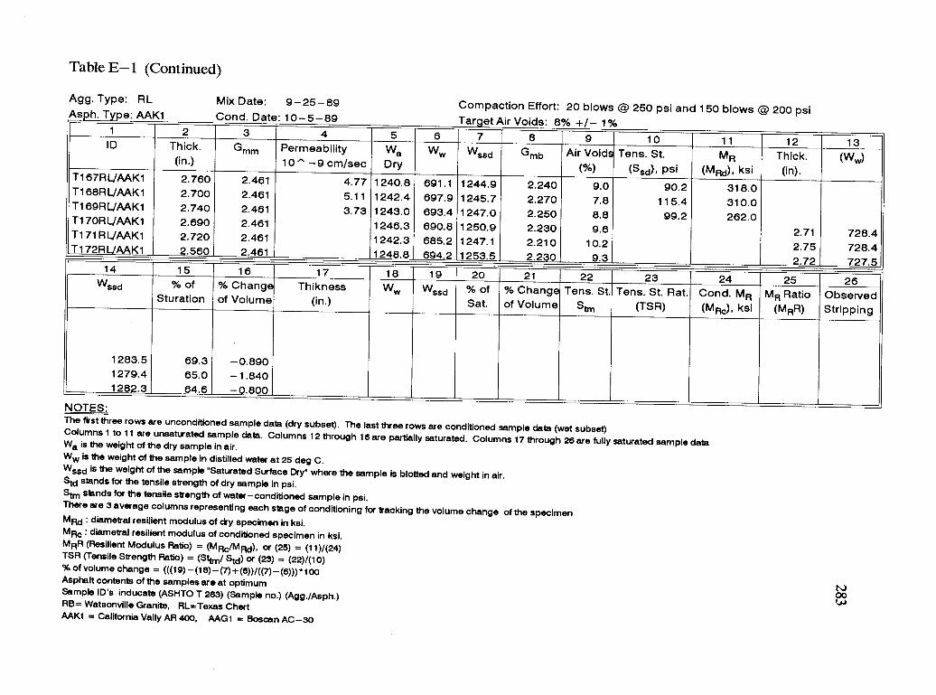
Table E- 1 (Continued)
Agg. Type: RLAs h. Type: AAK1
Mix Date: 9-25-89Cond. Date: 10-5-89
Compaction Effort: 20 blows @ 250 psi and 150 blows @ 200 psiTarget Air Voids: 8% +1- 1%
1 2 3 4 5 6 7 8 9 10 11 12 13ID Thick. G, Permeability Wa Ww Wssd Gmb Air Voids Tens. St. MR Thick. (Ww)(in.) 10 ^ -9 cm/sec Dry (%) (Ssd), psi (MRd), ksi (in).T167RL/AAK1 2.760 2.461 4.77 1240.8 691.1 1244.9 2.240 9.0 90.2 318.0T168RL/AAK1 2.700 2.461 5.11 1242.4 697.9 1245.7 2.270 7.8 115.4 310.0T169RL/AAK1 2.740 2.461 3.73 1243.0 693.4 1247.0 2.250 8.8 99.2 262.0T17ORL/AAK1 2.690 2.461 1246.3 690.8 1250.9 2.230 9.6 2.71 728.4T171RL/AAK1 2.720 2.461 1242.3 685.2 1247.1 2.210 10.2 2.75 728.4T172RL/AAK1 2.560 2.461 1248.8 694.2 1253.5 2.230 9.3 2.72 727.5
14 15 16 17 18 19 20 21 22 23 24 25 26Wssd % of % Change Thikness Ww Wssd % of % Change Tens. St. Tens. St. Rat. Cond. MR MR Ratio ObservedSturation of Volume (in.) Sat. of Volume St, (TSR) (MRS), ksi (MRR) Stripping
1283.5 69.3 -0.8901279.4 65.0 -1.8401282.3 64.6 -0.800
NOTES:The first three rows are unconditioned sampledata (dry subset). The last three rows are conditioned sample data (wet subset)Columns 1 to 11 are unsaturated sample data. Columns 12 through 16 are partially saturated. Columns 17 through 26 are fully saturated sample dataWa is the weight of the dry sample in air.Ww is the weight of the sample in distilled water at 25 deg C.Wssd is the weight of the sample "Saturated Surface Dry" where the sample is blotted and weight in air.Std stands for the tensile strength of dry sample inpsi.Stm stands for the tensile strength of water-conditioned sample in psi.There are 3 average columns representing each stage of conditioning for tracking the volume change of the specimenMRd : diametral resilient modulus of dry specimen in ksi.MRc : diametral resilient modulus of conditioned specimen in ksi.MRR (Resilient Modulus Ratio) = (MRc/MRd), or (25) = (11)/(24)TSR (Tensile Strength Ratio) = (Sttm/ Std) or (23) = (22)/(10)% of volume change = (((19) (18)- (7)+(6))/((7)- (6)))100Asphalt contents of the samples are at optimumSample ID's inducate (ASHTO T 283) (Sample no.) (Agg./Asph.)RB= Watsonville Granite, RL =Texas ChenAAK1 = California Vally AR 400, AAG1 = Boscan AC-30
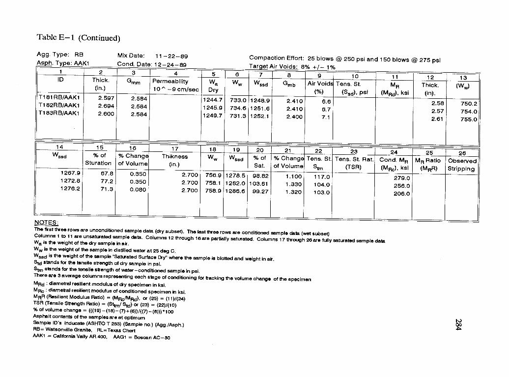
Table E- 1 (Continued)
Agg. Type: RBAs h. T e: AAK1
Mix Date: 11-22-89Cond. Date: 12-24-89
Compaction Effort: 25 blows @ 250 psi and 150 blows @ 275 psiTarget Air Voids: 8% +/- 1%
1 2 3 4 5 6 7 8 9 10 11 12 13ID Thick. Gmm Permeability Wa Ww Wssd Gmb Air Voids Tens. St. MR Thick. (Ww)(in.) 10 ^ -9 cm/sec Dry (%) (Sad). psi (MRd), ksi (in).T181RB/AAK1 2.597 2.584 1244.7 733.0 1248.9 2.410 6.6 2.58 750.2T182RB/AAK1 2.694 2.584 1245.9 734.6 1251.6 2.410 6.7 2.57 754.0T183RB/AAK1 2.600 2.584 1249.7 731.3 1252.1 2.400 7.1 2.61 755.0
14 15 16 17 18 19 20 21 22 23 24 25 26Wssd % of % Change Thikness Ww Wssd % of % Change Tens. St. Tens. St. Rat. Cond. MR MR Ratio ObservedSturation of Volume (in.) Sat. of Volume Stm (TSR) (MRb), ksi (MRR) Stripping1267.9 67.8 0.350 2.700 756.9 1278.5 98.82 1.100 117.0 279.01272.8 77.2 0.350 2.700 758.1 1282.0 103.61 1.330 104.0 256.01276.2 71.3 0.080 2.700 758.9 1286.6 99.27 1.320 103.0 206.0
NOTES:The first three rows are unconditioned sample data (dry subset). The last three rows are conditioned sample data (wet subset)Columns 1 to 11 are unsaturated sample data. Columns 12 through 16 are partially saturated. Columns 17 through 26 are fully saturated sample dataWa is the weight of the dry sample in air.Ww is the weight of the sample in distilled water at 25 deg C.Wssd is the weight of the sample "Saturated Surface Dry" where the sample is blotted and weight in air.Std stands for the tensile strength of dry sample in psi.Stm stands for the tensile strength of water-conditionedsample in psi.There are 3 average columns representing eachstage of conditioning for tracking the volume change of the specimenMRd : diametral resilient modulus of dry specimen in ksi.Mfic : diametral resilient modulus of conditioned specimen in ksi.MRR (Resilient Modulus Ratio) = (MRa/MRd), or (25) = (11)/(24)TSR (Tensile Strength Ratio) = (Sttm/ Std) or (23) = (22)/(10)% of volume change = (((19) -(18)- (7)+(6))/((7)- (6)))*100Asphalt contents of the samples are at optimumSample ID's inducate (ASHTO T 283) (Sample no.) (Agg./Asph.)RB= Watsonville Granite, RL=Texas ChartAAK1 = California Vally AR 400, AAG1 = Boscan AC-30
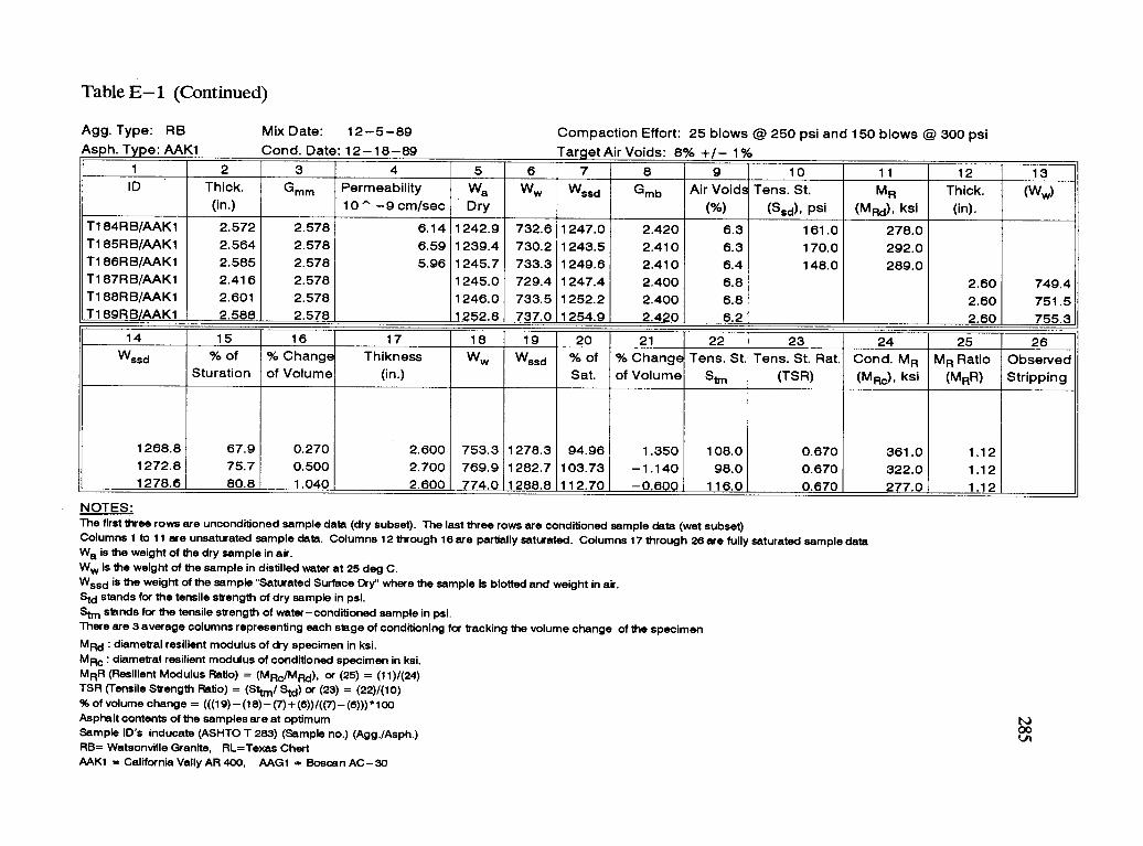
Table E- 1 (Continued)
Agg. Type: RBAs h. T e: AAK1
Mix Date: 12-5-89Cond. Date: 12-18-89
Compaction Effort: 25 blows @ 250 psi and 150 blows @ 300 psiTarget Air Voids: 8% +/- 1%
1 2 3 4 5 6 7 8 9 10 11 12 13ID Thick. G Permeability Wa Ww Wssd Gmb Air Voids Tens. St. MR Thick. (Ww)
(in.) 10 ^ -9 cm/sec Dry (%) (Ssd), psi (MRd), ksi (in).T184RB/AAK1 2.572 2.578 6.14 1242.9 732.6 1247.0 2.420 6.3 161.0 278.0T185RB/AAK1 2.564 2.578 6.59 1239.4 730.2 1243.5 2.410 6.3 170.0 292.0T186RB/AAK1 2.585 2.578 5.96 1245.7 733.3 1249.6 2.410 6.4 148.0 289.0T187RB/AAK1 2.416 2.578 1245.0 729.4 1247.4 2.400 6.8 2.60 749.4T188RB/AAK1 2.601 2.578 1246.0 733.5 1252.2 2.400 6.8 2.60 751.5T189RB/AAK1 2.588 2.578 1252.8 737.0 1254.9 2.420 6.2 2.60 755.3
14 15 16 17 18 19 20 21 22 23 24 25 26Wssd % of % Change Thikness Ww Wssd % of % Change Tens. St. Tens. St. Rat. Cond. MR MR Ratio Observed
Sturation of Volume (in.) Sat. of Volume Sim (TSR) (MRd), ksi (MRR) Stripping
1268.8 67.9 0.270 2.600 753.3 1278.3 94.96 1.350 108.0 0.670 361.0 1.121272.8 75.7 0.500 2.700 769.9 1282.7 103.73 -1.140 98.0 0.670 322.0 1.121278.6 80.8 1.040 2.600 774.0 1288.8 112.70 -0.600 116.0 0.670 277.0 1.12
NOTES:The first three rows are unconditioned sample data (dry subset). The last three rows are conditioned sample data (wet subset)Columns 1 to 11 are unsaturated sample data. Columns 12 through 16 are partially saturated. Columns 17 through 26 are fully saturated sample dataWa is the weight of the dry sample in air.Ww is the weight of the sample in distilled water at 25 deg C.Wssd is the weight of the sample "Saturated Surface Dry" where the sample is blotted and weight in air.Std stands for the tensile strength of dry sample in psi.Stm stands for the tensile strength of water-conditioned sample in psi.There are 3 average columns representing each stage of conditioning for tracking the volume change of the specimenMRd : diametral resilient modulus of dry specimen in ksi.MRc : diametral resilient modulus of conditioned specimen in ksi.MRR (Resilient Modulus Ratio) = (11/44RcThARd), or (25) = (11)/(24)TSR (Tensile Strength Ratio) = (Sttm/ Std) or (23) = (22)/(10)% of volume change = (((19)- (18)- (7)+ (8))/((7)- (6)))*100Asphalt contents of the samples are at optimumSample ID's inducate (ASHTO T 283) (Sample no.) (Agg./Asph.)RB= Watsonville Granite, RL=Texas ChertAAK1 = California Vally AR 400, AAG1 = Bosoan AC-30
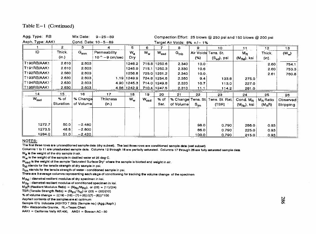
Table E- 1 (Continued)
Agg. Type: RBAs h. T e: AAK1
Mix Date: 9-25-89Cond. Date: 10-5-89
Compaction Effort: 25 blows @ 250 psi and 150 blows @ 200 psiTarget Air Voids: 8% +/- 1%
1 2 3 4 5 6 7 8 9 10 11 12 13ID Thick. Gmm Permeability Wa Ww Wssd Gmb Air Voids Tens. St. MR Thick. (WIN)
(in.) 10 '' -9 cm/sec Dry (%) (Ssd), psi (MRd), ksi (in).T190RB/AAK1 2.610 2.603 1246.2 718.8 1250.6 2.340 10.0 2.60 754.1T191RB/AAK1 2.610 2.603 1245.9 715.1 1250.3 2.330 10.6 2.60 753.3T192RB/AAK1 2.560 2.603 1256.8 725.0 1261.2 2.340 10.0 2.61 760.8T193RB/AAK1 2.630 2.603 1.19 1249.9 724.8 1254.6 2.360 9.4 133.8 275.0T194RB/AAK1' 2.630 2.603 4.90 1245.3 714.0 1249.8 2.320 10.7 113.0 227.0T195RB/AAK1 2.630 2.603 4.86 1242.9 710.4 1247.5 2.310 11.1 114.2 281.0
14 15 16 17 18 19 20 21 22 23 24 25 26Wssd % of % Change Thikness Ww Wssd % of % Change Tens. St. Tens. St. Rat. Cond. MR MR Ratio Observed
Sturation of Volume (in.) Sat. of Volume Stm (TSR) (MR,), ksi (MRR) Stripping
1272.7 50.0 -2.480 98.0 0.790 286.0 0.931273.5 48.8 -2.800 86.0 0.790 225.0 0.931284.0 51.0 -2.420 100.0 0.790 215.0 0.93
NOTES:The first three rows are unconditioned sample data (dry subset). The last three rows are conditioned sample data (wet subset)Columns 1 to 11 are unsaturated sample data. Columns 12 through 16 are partially saturated. Columns 17 through 26 are fully saturated sample dataWa is the weight of the dry sample in air.Ww is the weight of the sample in distilled water at 25 deg C.Wssd is the weight of the sample "Saturated Surface Dry" where the sample is blotted and weight in air.Std stands for the tensile strength of dry sample in psi.Stm stands for the tensile strength of water -conditioned sample in psi.There are 3 average columns representing each stage of conditioning for tracking the volume change of the specimenMRd : diametral resilient modulus of dry specimen in ksi.MRc : diametral resilient modulus of conditioned specimen in ksi.MRR (Resilient Modulus Ratio) = (MRb/MRd), or (25) = (11)1(24)TSR (Tensile Strength Ratio) = (Sttm/ Std) or (23) = (22)1(10)% of volume change = (((19) - (18) (7)+(6))/((7)- (6)))*100Asphalt contents of the samples are at optimumSample ID's inducate (ASHTO T 283) (Sample no.) (Agg./Asph.)RB= Watsonville Granite, RL=Texas ChertAAK1 = California Vally AR 400, AAG1 = Boscan AC-30
00ON

Table E- 1 (Continued)
Agg. Type: RBAs h. T e: AAG1
Mix Date: 11 -21 -89Cond. Date: 12-26-89
Compaction Effort: 25 blows @ 250 psi and 150 blows @ 175 psiTarget Air Voids: 8% +/- 1%
1 2 3 4 5 6 7 8 9 10 11 12 13ID Thick. Gmm Permeability Wa Ww Wssd Gmb Air Voids Tens. St. MR Thick. (Ww)
(in.) 10 ^ -9 cm/sec Dry (%) (Ssd), psi (MRd), ksi (in).T201RB/AAG1 2.626 2.574 4.65 1251.8 731.5 1256.6 2.380 7.4 165.0 256.0T202RB/AAG1 2.652 2.574 9.32 1253.9 732.6 1261.1 2.370 7.8 111.0 211.0T203RB/AAG1 2.619 2.574 6.05 1251.8 729.9 1255.2 2.380 7.4 162.0 255.0T204RB/AAG1 2.613 2.574 1251.1 733.9 1257.0 2.390 7.1 2.61 751.0T205RB/AAG1 2.594 2.574 1237.2 720.6 1240.7 2.380 7.6 2.59 746.1T206RB/AAG1 2.610 2.574 1246.4 729.4 1250.7 2.390 7.1 2.60 751.0
14 15 16 17 18 19 20 21 22 23 24 25 26Wssd % of % Change Thikness Ww Wssd % of % Change Tens. St. Tens. St. Rat. Cond. MR MR Ratio Observed
Sturation of Volume (in.) Sat. of Volume Stm (TSR) (MRa), ksi (MRR) Stripping
1276.5 68.6 0.460 2.600 755.9 1286.2 94.74 1.380 75.8 0.510 148.0 0.621266.2 73.5 0.000 2.600 747.7 1274.7 95.06 1.330 64.4 0.510 154.0 0.621272.7 70.9 0.080 2.600 753.8 1282.2 96.57 1.360 81.3 0.510 144.0 0.62
NOTES:The first three rows are unconditioned sample data (dry subset). The last three rows are conditioned sample data (wet subset)Columns 1 to 11 are unsaturated sample data. Columns 12 through 16 are partially saturated. Columns 17 through 26 are fully saturated sample dataWa is the weight of the dry sample in air.Ww is the weight of the sample in distilled water at 25 deg C.Wssd is the weight of the sample "Saturated Surface Dry" where the sample is blotted and weight in air.Std stands for the tensile strength of dry sample in psi.Sur, stands for the tensile strength of water-conditioned sample in psi.There are 3 average columns representing each stage of conditioning for tracking the volume change of the specimenMRc : diametral resilient modulus of dry specimen in ksi.MRc : diametral resilient modulus of conditioned specimen in ksi.MRR (Resilient Modulus Ratio) = (MRc/MRd), or (25) = (11)/(24)TSR (Tensile Strength Ratio) = (Sttrn/ Std) or (23) = (22)/(10)% of volume change = (((19)- (18)- (7)+(6))/((7) (6)))100Asphalt contents of the samples are at optimumSample ID's inducate (ASHTO T 283) (Sample no.) (Agg./Asph.)RB= Watsonville Granite, RL=Texas ChartAAK1 = California Vally AR 400, AAG1 = Boscan AC-30
t.)00
288
APPENDIX F
PERMEABILITY PROTOCOL
Scope
This test method is for laboratory measurement of permeability of compactedbituminous mixtures. This method measures the rate at which air can be drawn(vacuum system) through bituminous mixtures.
This procedure takes advantage of previous experience, providing accuracy andsimplicity, and reducing the possibility of asphalt contamination, specimendeformation, and the other deficiencies often found with other methods. In thisprocedure, the middle one-third of the specimen's circumference is coated withsilicone and then enveloped with a cylindrical rubber membrane 1.5 inches high toprovide a smooth surface, then cured overnight. A pressure differential is appliedacross the specimen by connecting the specimen setup to a vacuum pump. Fordifferent vacuum readings, the rate of air flow through the specimen is reported.Permeability is determined by calculating the rate of air flow and pressuredifferential.
289
Referenced Documents
ASTM Standards: D 3637 Permeability of Bituminous Mixtures
Definitions
Permeability as defined by Wyckoff, et al 1933: Permeability (K) is the volume offluid (Q) of unit viscosity (h) passing in unit time (At) through a unit cross section(A) of a porous medium of length (L) under the influence of a unit-pressure gradient(AP)
Q II LKA Ap At
Summary of Method
From the permeability definition, air permeability can be measured by creating aknown pressure differential through the specimen by measuring the rate of air flowfor a known period of time.
In order for the air flow to pass only through the specimen, the specimen wall mustbe sealed. Goode and Lufsey (1965) used paraffin for sealing to prevent leakagebetween the specimen wall and the membrane. However, this method destroys thespecimen for further use by contaminating the asphalt.
Another method is to place the specimen in a cylindrical rubber membrane fastenedto a hollow metal cylinder with hose clamps. This method does not totally preventleakage between the specimen wall and the membrane, especially with coarsemixtures. Another disadvantage of this method is that deformation of the specimenmay be caused by the air pressure in the membrane.
Kumar and Goetz (1977) developed a different technique to prevent leakage. Thespecimen is placed between two collars (lower collar and upper collar) and coatedwith silicone rubber sealant all around the specimen and part of both collars in orderto bind the collars to the specimen. This method prevents the leakage through thespecimen wall, but it is rather involved and time consuming.
The OSU procedure is simple and eliminates the above problems while stillpreventing leakage. The procedure is outlined in the following sections.
290
Significance and Use
This method can be used only for a laboratory test for mix design purposes.
The following ideal test conditions are prerequisites for the laminar flow of airthrough porous medium under constant-head conditions:
Continuity of flow with no volume change during a test.Flow with the voids fully saturated with the air.Flow in the steady state with no changes in pressuregradient, andDirect proportionality of velocity of flow with pressure gradientsbelow certain values, at which turbulent flow starts.
Apparatus
Figure F-1 shows the equipment set-up. The set-up is capable of accommodating arange of specimen sizes.
Test Specimens
Since this test is part of the Moisture Induced Damage Study, the dry subset forAASHTO T 283 will be tested for permeability.
Procedure
Place the specimen on specimen holder and seal the middle (Fig. F-2) specimen wallby applying silicone to the middle 1.5 inch, and enveloping the silicone seal with acylindrical rubber membrane for the same width (1.5 inches). Cure the specimenovernight.
Place the specimen in the triaxial apparatus and envelope the specimen with acylindrical rubber membrane, long enough to envelope the sample base, upper andlower porous teflon, and sample cap, then tie the assembly using rubber bands ateach end.
Attach the vacuum outlet to the manometer and vacuum pump, and to the inlet tothe flowmeter. To check for leaks, open valve (a) in Figure B-2 (Appendix B) andclose the flowmeter until the manometer reads more than 250 mm Hg, by adjustingthe vacuum level with the vacuum regulator.

291
Close valve (a) in Figure B-2 and watch the manometer reading. If manometerreading does not decrease, the system is air tight and ready for testing.
Open the flow meter and valve (a), apply the desired pressure difference (manometerreading) by adjusting the vacuum regulator, then take the rate of air flow, readingthrough the specimen from the air flow meter. Repeat for several different pressuresand calculate the pressure differential.
Calculation
The permeability of a porous mediumdefined in fundamental units, is:
where:
K g Q LA(P1 P2)
K = permeability in centimeters per second.g = viscosity of fluid in poises,0 = rate of flow, cubic centimeters per second.L = height of sample, centimetersA = area of sample in square centimetersP1 - P2 = pressure difference, dynes per square centimeter.
The above formula was modified by Kumar and Goetz as shown below:
For specimen 4 inch (10.16 cm) in diameterA a test temperature of 20°C (68°F) anda value for A at 20°C (68°F) of 1.813X10-* poises, the above formula reduces to:
K = (3.812 x 0-11 x R x H)/AP
where:R = rate of airflow in ml per minuteH = height of specimen in centimeters, andAP = pressure differential in centimeters of water
By using the slope (S) of the straight line portion of the curve obtained from the plotof rate of airflow (R) (y axis) versus pressure differential (AP) (x axis), this reducesthe above formula to:
292
K = 3.812 x 10-"xSxH
Since the pressure difference is measured in millimeters of mercury (mm Hg) andthe rate of airflow in cubic foot per hour (ft3 /hr) the following conversion factors areused:
1.0 ft3 /hr = 471.9 cm3 /min.1.0 mm HG = 1.868 inch of water
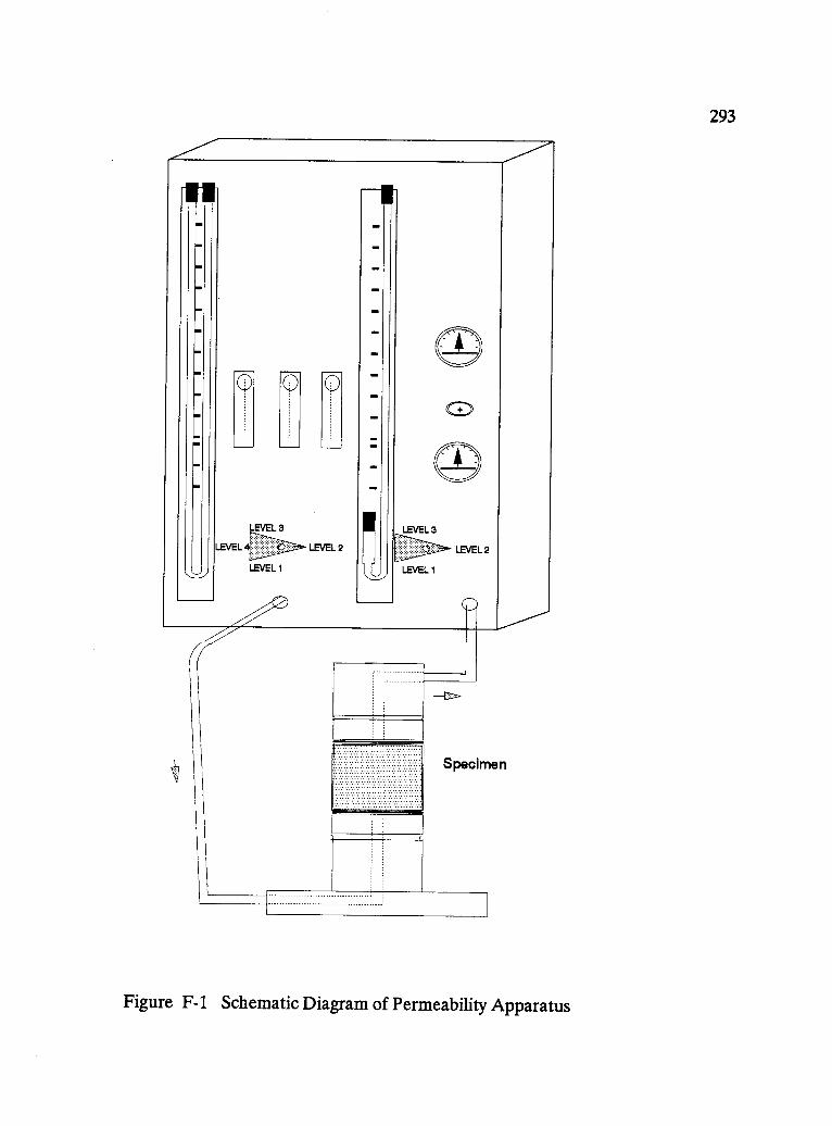
293
0 0 0
LEVEL 3
LEVEL LEVEL 2
LEVEL 1
LEVEL 3
LEVEL 1
LEVEL 2
Specimen
Figure F-1 Schematic Diagram of Permeability Apparatus

294
a) Specimen sealing for 1.5" of the middle
b) Rubber membrane fastening to specimen
Figure F-2 Permeability Sealing of Compacted Asphalt Mixtures
295
APPENDIX G
STANDARD TEST METHOD FOR DYNAMIC MODULUS OF ASPHALTMIXTURESASTM D 3497
Scope
This test method covers procedures for preparing and testing asphalt mixtures todetermine dynamic modulus values. The procedure described covers a range of bothtemperatures and loading frequencies. The minimum recommended test seriesconsists of testing at 41, 77, and 104°F (5, 25, and 40°C) at loading frequencies of1, 4, and 15 Hz for each temperature.
This method is applicable to asphalt paving mixtures similar to mixes 3A, 4A, 5A,6A, and 7A, as defined by Specification D 3515.
This standard may involve hazardous materials, operations, and equipment. Thisstandard does not purport to address all of the safety problems associated with itsuse. It is the responsibility of whoever uses this standard to consult and establishappropriate safety and health practices and determine the applicability of regulatorylimitations prior to use.
Referenced Documents
ASTM Standards:
C 617 Practice for Capping Cylindrical Concrete SpecimensD 3496 Method for Preparation of Bituminous Mixture

296
Specimens for Dynamic Modulus Testing
D 3515 Specifications for Hot-Mixed, Hot-Laid Bituminous
Paving Mixtures
Definitions
Dynamic modulus - the absolute value of the complex modulus that defines theelastic properties of a linear viscoelastic material subjected to a sinusoidal loading,
E*
Complex modulus - a complex number that defines the relationship between stressand strain for a linear viscoelastic material, E*.
Linear material - a material whose stress to strain ratio is independent of the loadingstress applied.
Summary of Method
A sinusoidal (haversine) axial compression stress is applied to a specimen of asphaltconcrete at a given temperature and loading frequency. The resulting recoverableaxial strain response of the specimen is measured and used to calculate dynamicmodulus.
Significance and Use
The values of dynamic modulus can be used for both asphalt paving mixture designand asphalt pavement thickness design.
Apparatus
Testing Machine - An electro-hydraulic testing machine with a function generatorcapable of producing a haversine wave form has proven to be most suitable for usein dynamic modulus testing. The testing machine should have the capability ofapplying the loads over a range of frequencies from 0.1 to 20 Hz and stress levels upto 100 psi (690 kPa).
Temperature-Control System - The temperature-control system should be capable ofa temperature range from 32 to 120 ± 1°F (0 to 50 ± 0.5 °C). The temperature
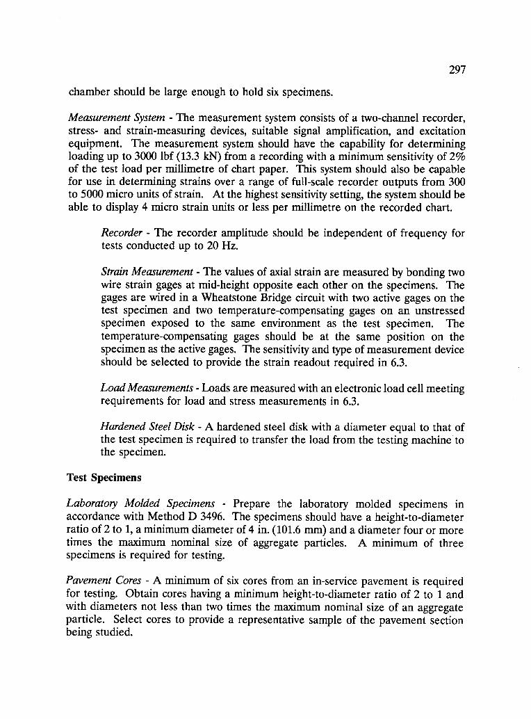
297
chamber should be large enough to hold six specimens.
Measurement System The measurement system consists of a two-channel recorder,stress- and strain-measuring devices, suitable signal amplification, and excitationequipment. The measurement system should have the capability for determiningloading up to 3000 lbf (13.3 IN) from a recording with a minimum sensitivity of 2%of the test load per millimetre of chart paper. This system should also be capablefor use in determining strains over a range of full-scale recorder outputs from 300to 5000 micro units of strain. At the highest sensitivity setting, the system should beable to display 4 micro strain units or less per millimetre on the recorded chart.
Recorder - The recorder amplitude should be independent of frequency fortests conducted up to 20 Hz.
Strain Measurement - The values of axial strain are measured by bonding twowire strain gages at mid-height opposite each other on the specimens. Thegages are wired in a Wheatstone Bridge circuit with two active gages on thetest specimen and two temperature-compensating gages on an unstressedspecimen exposed to the same environment as the test specimen. Thetemperature-compensating gages should be at the same position on thespecimen as the active gages. The sensitivity and type of measurement deviceshould be selected to provide the strain readout required in 6.3.
Load Measurements - Loads are measured with an electronic load cell meetingrequirements for load and stress measurements in 6.3.
Hardened Steel Disk - A hardened steel disk with a diameter equal to that ofthe test specimen is required to transfer the load from the testing machine tothe specimen.
Test Specimens
Laboratory Molded Specimens - Prepare the laboratory molded specimens inaccordance with Method D 3496. The specimens should have a height-to-diameterratio of 2 to 1, a minimum diameter of 4 in. (101.6 mm) and a diameter four or moretimes the maximum nominal size of aggregate particles. A minimum of threespecimens is required for testing.
Pavement Cores A minimum of six cores from an in-service pavement is requiredfor testing. Obtain cores having a minimum height-to-diameter ratio of 2 to 1 andwith diameters not less than two times the maximum nominal size of an aggregateparticle. Select cores to provide a representative sample of the pavement sectionbeing studied.
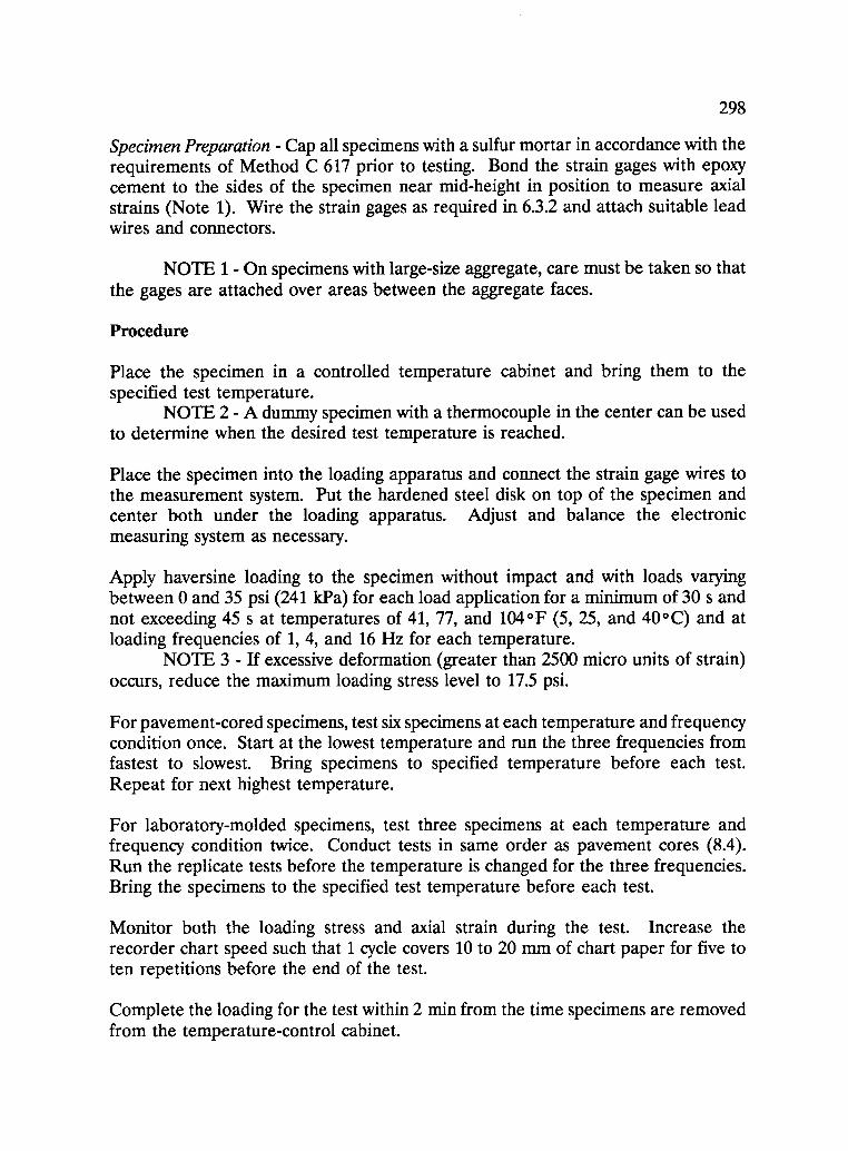
298
Specimen Preparation Cap all specimens with a sulfur mortar in accordance with therequirements of Method C 617 prior to testing. Bond the strain gages with epoxycement to the sides of the specimen near mid-height in position to measure axialstrains (Note 1). Wire the strain gages as required in 6.3.2 and attach suitable leadwires and connectors.
NOTE 1- On specimens with large-size aggregate, care must be taken so thatthe gages are attached over areas between the aggregate faces.
Procedure
Place the specimen in a controlled temperature cabinet and bring them to thespecified test temperature.
NOTE 2 A dummy specimen with a thermocouple in the center can be usedto determine when the desired test temperature is reached.
Place the specimen into the loading apparatus and connect the strain gage wires tothe measurement system. Put the hardened steel disk on top of the specimen andcenter both under the loading apparatus. Adjust and balance the electronicmeasuring system as necessary.
Apply haversine loading to the specimen without impact and with loads varyingbetween 0 and 35 psi (241 kPa) for each load application for a minimum of 30 s andnot exceeding 45 s at temperatures of 41, 77, and 104 °F (5, 25, and 40 °C) and atloading frequencies of 1, 4, and 16 Hz for each temperature.
NOTE 3 - If excessive deformation (greater than 2500 micro units of strain)occurs, reduce the maximum loading stress level to 17.5 psi.
For pavement-cored specimens, test six specimens at each temperature and frequencycondition once. Start at the lowest temperature and run the three frequencies fromfastest to slowest. Bring specimens to specified temperature before each test.Repeat for next highest temperature.
For laboratory-molded specimens, test three specimens at each temperature andfrequency condition twice. Conduct tests in same order as pavement cores (8.4).Run the replicate tests before the temperature is changed for the three frequencies.Bring the specimens to the specified test temperature before each test.
Monitor both the loading stress and axial strain during the test. Increase therecorder chart speed such that 1 cycle covers 10 to 20 mm of chart paper for five toten repetitions before the end of the test.
Complete the loading for the test within 2 min from the time specimens are removedfrom the temperature-control cabinet.
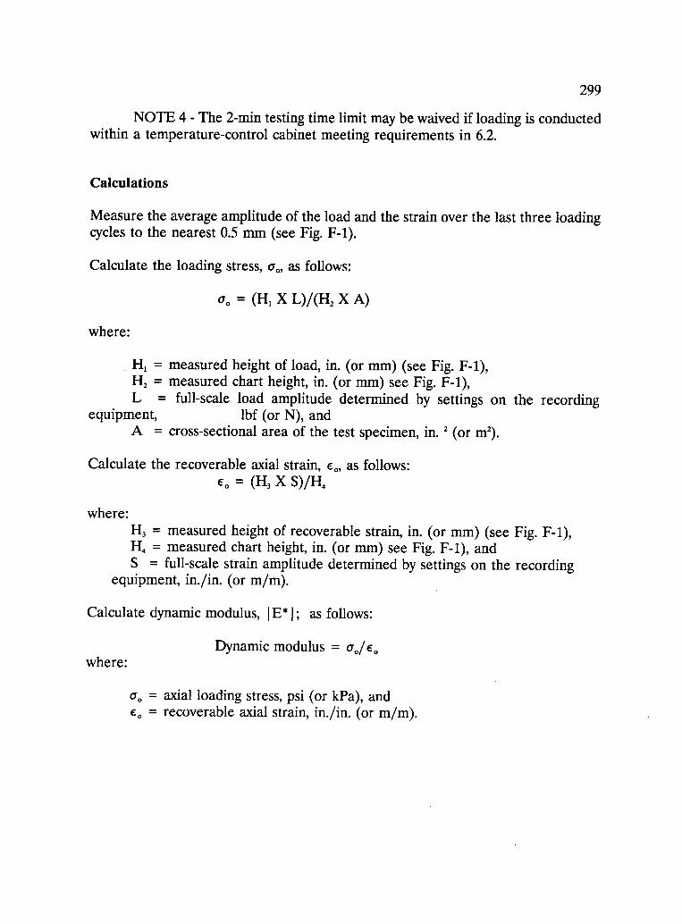
299
NOTE 4 - The 2-min testing time limit may be waived if loading is conductedwithin a temperature-control cabinet meeting requirements in 6.2.
Calculations
Measure the average amplitude of the load and the strain over the last three loadingcycles to the nearest 0.5 mm (see Fig. F-1).
Calculate the loading stress, a., as follows:
a. = (H1 X L)/(11, X A)
where:
H, = measured height of load, in. (or mm) (see Fig. F-1),H2 = measured chart height, in. (or mm) see Fig. F-1),L = full-scale load amplitude determined by settings on the recording
equipment, lbf (or N), andA = cross-sectional area of the test specimen, in. 2 (or m2).
Calculate the recoverable axial strain, E., as follows:e. = (H3 X S)/H4
where:H3 = measured height of recoverable strain, in. (or mm) (see Fig. F-1),11, = measured chart height, in. (or mm) see Fig. F-1), andS = full-scale strain amplitude determined by settings on the recording
equipment, in./in. (or m/m).
Calculate dynamic modulus, I E* I ; as follows:
where:Dynamic modulus = ao/e.
a. = axial loading stress, psi (or kPa), ande. = recoverable axial strain, in./in. (or m/m).
300
Report
Report the average dynamic modulus at temperatures or 41, 77, and 104°F (5, 25,and 40°C) for 1, 4, and 16-Hz loading frequencies at each temperature.
Precision
11.1 This test method shall not be used for Specification purposes.

301
Figure G-1 Recording of Load and Strain