Test Guideline No. 425Acute Oral Toxicity: Up-and-Down

Procedure

30 June 2022

OECD Guidelines for the Testing of Chemicals

Section 4Health effects

OECD/OCDE 425 Adopted:

16 October 2008 Corrected:

30 June 2022 (caging, parag. 17)

© OECD, (2022)

You are free to use this material subject to the terms and conditions available at http://www.oecd.org/termsandconditions/.

OECD GUIDELINE FOR THE TESTING OF CHEMICALS

Acute Oral Toxicity – Up-and-Down-Procedure (UDP)

INTRODUCTION

1. OECD guidelines for the Testing of Chemicals are periodically reviewed in the light of scientific

progress or changing assessment practices. The concept of the up-and-down testing approach was first

described by Dixon and Mood (1)(2)(3)(4). In 1985, Bruce proposed to use an up-and-down procedure

(UDP) for the determination of acute toxicity of chemicals (5). There exist several variations of the up-and-

down experimental design for estimating an LD50. This guideline is based on the procedure of Bruce as

adopted by ASTM in 1987 (6) and revised in 1990. A study comparing the results obtained with the UDP,

the conventional LD50 test and the Fixed Dose Procedure (FDP, OECD Test Guideline 420) was published

in 1995 (7). Since the early papers of Dixon and Mood, papers have continued to appear in the biometrical

and applied literature, examining the best conditions for use of the approach (8)(9)(10)(11). Based on the

recommendations of several expert meetings in 1999, an additional revision was considered timely

because: i) international agreement had been reached on harmonized LD50 cut-off values for the

classification of chemical substances, ii) testing in one sex (usually females) is generally considered

sufficient, and iii) in order for a point estimate to be meaningful, there is a need to estimate confidence

intervals (CI).

2. The test procedure described in this Guideline is of value in minimizing the number of animals

required to estimate the acute oral toxicity of a chemical. In addition to the estimation of LD50 and

confidence intervals, the test allows the observation of signs of toxicity. Revision of Test Guideline 425

was undertaken concurrently with revisions to the Test Guidelines 420 and 423.

3. Guidance on the selection of the most appropriate test method for a given purpose can be found

in the Guidance Document on Oral Toxicity Testing (12). This Guidance Document also contains additional

information on the conduct and interpretation of Guideline 425.

4. Definitions used in the context of this Guideline are set out in Annex 1.

INITIAL CONSIDERATIONS

5. The testing laboratory should consider all available information on the test substance prior to

conducting the study. Such information will include the identity and chemical structure of the test

substance; its physical chemical properties; the results of any other in vitro or in vivo toxicity tests on the

substance; toxicological data on structurally related substances or similar mixtures; and the anticipated

OECD/OCDE 425

© OECD, (2022)

use(s) of the substance. This information is useful to determine the relevance of the test for the protection

of human health and the environment, and will help in the selection of an appropriate starting dose.

6. The method permits estimation of an LD50 with a confidence interval and the results allow a

substance to be ranked and classified according to the Globally Harmonised System for the classification

of chemicals, which cause acute toxicity (16).

7. When no information is available to make a preliminary estimate of the LD50 and the slope of the

dose-response curve, results of computer simulations have suggested that starting near 175 mg/kg and

using half-log units (corresponding to a dose progression of factor 3.2) between doses will produce the

best results. This starting dose should be modified if the substance is likely to be highly toxic. The half-

log spacing provides for a more efficient use of animals, and increases accuracy in the prediction of the

LD50 value. Because the method has a bias toward the starting dose, it is essential that initial dosing

occur below the estimated LD50. (See paragraphs 32 and Annex 2 for discussion of dose sequences and

starting values). However, for chemicals with large variability (i.e., shallow dose-response slopes), bias

can still be introduced in the lethality estimates and the LD50 will have a large statistical error, similar to

other acute toxicity methods. To correct for this, the main test includes a stopping rule keyed to properties

of the estimate rather than a fixed number of test observations (see paragraph 33).

8. The method is easiest to apply to materials that produce death within one or two days. The method

would not be practical to use when considerably delayed death (five days or more) can be expected.

9. Computers are used to facilitate animal-by-animal calculations that establish testing sequences

and provide final estimates.

10. Test substances, at doses that are known to cause marked pain and distress due to corrosive or

severely irritant actions, need not be administered. Moribund animals or animals obviously in pain or

showing signs of severe and enduring distress shall be humanely killed, and are considered in the

interpretation of the test results in the same way as animals that died on test. Criteria for making the

decision to kill moribund or severely suffering animals, and guidance on the recognition of predictable or

impending death are the subject of a separate OECD Guidance Document (13).

11. A limit test can be used efficiently to identify chemicals that are likely to have low toxicity.

PRINCIPLE OF THE LIMIT TEST

12. The Limit Test is a sequential test that uses a maximum of 5 animals. A test dose of 2000, or

exceptionally 5000 mg/kg, may be used. The procedures for testing at 2000 and 5000 mg/kg are slightly

different (see paragraphs 23-25 for limit test at 2000 mg/kg and paragraphs 26-30 for limit test at 5000

mg/kg). The selection of a sequential test plan increases the statistical power and also has been made to

intentionally bias the procedure towards rejection of the limit test for compounds with LD50s near the limit

dose; i.e., to err on the side of safety. As with any limit test protocol, the probability of correctly classifying

a compound will decrease as the actual LD50 more nearly resembles the limit dose.

PRINCIPLE OF THE MAIN TEST

13. The main test consists of a single ordered dose progression in which animals are dosed, one at a

time, at a minimum of 48-hour intervals. The first animal receives a dose a step below the level of the best

estimate of the LD50. If the animal survives, the dose for the next animal is increased by [a factor of] 3.2

times the original dose; if it dies, the dose for the next animal is decreased by a similar dose progression.

(Note: 3.2 is the default factor corresponding to a dose progression of one half log unit. Paragraph 32

OECD/OCDE 425

© OECD, (2022)

provides further guidance for choice of dose spacing factor.) Each animal should be observed carefully

for up to 48 hours before making a decision on whether and how much to dose the next animal. That

decision is based on the 48-hour survival pattern of all the animals up to that time. (See paragraphs 31

and 35 on choice of dosing interval). A combination of stopping criteria is used to keep the number of

animals low while adjusting the dosing pattern to reduce the effect of a poor starting value or low slope

(see paragraph 34). Dosing is stopped when one of these criteria is satisfied (see paragraphs 33 and 41),

at which time an estimate of the LD50 and a confidence interval are calculated for the test based on the

status of all the animals at termination. For most applications, testing will be completed with only 4 animals

after initial reversal in animal outcome. The LD50 is calculated using the method of maximum likelihood

(14)(15). (See paragraphs 41 and 43.)

14. The results of the main test procedure serve as the starting point for a computational procedure to

provide a confidence interval estimate where feasible. A description of the basis for this CI is outlined in

paragraph 45.

DESCRIPTION OF THE METHOD

Selection of Animal Species

15. The preferred rodent species is the rat although other rodent species may be used. Normally

female rats are used (12). This is because literature surveys of conventional LD50 tests show that usually

there is little difference in sensitivity between sexes, but in those cases where differences are observed,

females are generally slightly more sensitive (7). However, if knowledge of the toxicological or toxicokinetic

properties of structurally related chemicals indicates that males are likely to be more sensitive then this

sex should be used. When the test is conducted in males, adequate justification should be provided.

16. Healthy young adult animals of commonly used laboratory strains should be employed. Females

should be nulliparous and non-pregnant. At the commencement of its dosing, each animal should be

between 8 and 12 weeks old and its weight should fall in an interval within ± 20 % of the mean initial weight

of any previously dosed animals.

Housing and Feeding Conditions

17. The temperature in the experimental animal room should be 22°C (± 3°C). Although the relative

humidity should be at least 30 % and preferably not exceed 70 % other than during room cleaning, the aim

should be 50-60%. Lighting should be artificial, the sequence being 12 hours light and 12 hours dark. At

48 hours after dosing, animals may be returned to group housing unless there are reasons to house

individually (e.g. there is concern that contact with other animals could increase stress due to the severity

of the signs of toxicity). However, the time that the animals are housed individually should be minimised

as appropriate, for animal welfare reasons. For feeding, conventional rodent laboratory diets may be used

with an unlimited supply of drinking water.

Preparation of Animals

18. The animals are randomly selected, marked to permit individual identification, and kept in their

cages for at least 5 days prior to dosing to allow for acclimatisation to the laboratory conditions. As with

OECD/OCDE 425

© OECD, (2022)

other sequential test designs, care must be taken to ensure that animals are available in the appropriate

size and age range for the entire study.

Preparation of Doses

19. In general test substances should be administered in a constant volume over the range of doses

to be tested by varying the concentration of the dosing preparation. Where a liquid end product or mixture

is to be tested, however, the use of the undiluted test substance, i.e., at a constant concentration, may be

more relevant to the subsequent risk assessment of that substance, and is a requirement of some

regulatory authorities. In either case, the maximum dose volume for administration must not be exceeded.

The maximum volume of liquid that can be administered at one time depends on the size of the test animal.

In rodents, the volume should not normally exceed 1 ml/100g of body weight; however in the case of

aqueous solutions, 2 ml/100g body weight can be considered. With respect to the formulation of the dosing

preparations, the use of an aqueous solution/suspension/emulsion is recommended wherever possible,

followed in order of preference by a solution/suspension/emulsion in oil (e.g. corn oil) and then possibly

solution in other vehicles. For vehicles other than water the toxicological characteristics of the vehicle

should be known. Doses must be prepared shortly prior to administration unless the stability of the

preparation over the period during which it will be used is known and shown to be acceptable.

PROCEDURE

Administration of Doses

20. The test substance is administered in a single dose by gavage using a stomach tube or a suitable

intubation cannula. In the unusual circumstance that a single dose is not possible, the dose may be given

in smaller fractions over a period not exceeding 24 hours.

21. Animals should be fasted prior to dosing (e.g., with the rat, food but not water should be witheld

overnight; with the mouse, food but not water should be withheld for 3-4 hours). Following the period of

fasting, the animals should be weighed and the test substance administered. The fasted body weight of

each animal is determined and the dose is calculated according to the body weight. After the substance

has been administered, food may be withheld for a further 3-4 hours in rats or 1-2 hours in mice. Where

a dose is administered in fractions over a period of time, it may be necessary to provide the animals with

food and water depending on the length of the period.

Limit test and Main Test

22. The limit test is primarily used in situations where the experimenter has information indicating that

the test material is likely to be nontoxic, i.e., having toxicity below regulatory limit doses. Information about

the toxicity of the test material can be gained from knowledge about similar tested compounds or similar

tested mixtures or products, taking into consideration the identity and percentage of components known to

be of toxicological significance. In those situations where there is little or no information about its toxicity,

or in which the test material is expected to be toxic, the main test should be performed.

OECD/OCDE 425

© OECD, (2022)

Limit Test

Limit Test at 2000 mg/kg

23. Dose one animal at the test dose. If the animal dies, conduct the main test to determine the LD50.

If the animal survives, dose four additional animals sequentially so that a total of five animals are tested.

However, if three animals die, the limit test is terminated and the main test is performed. The LD50 is

greater than 2000 mg/kg if three or more animals survive. If an animal unexpectedly dies late in the study,

and there are other survivors, it is appropriate to stop dosing and observe all animals to see if other animals

will also die during a similar observation period (see paragraph 31 for initial observation period). Late

deaths should be counted the same as other deaths. The results are evaluated as follows (O=survival,

X=death).

24. The LD50 is less than the test dose (2000 mg/kg) when three or more animals die.

O XO XX

O OX XX

O XX OX

O XX X

If a third animal dies, conduct the main test.

25. Test five animals. The LD50 is greater than the test dose (2000 mg/kg) when three or more animals

survive.

O OO OO

O OO XO

O OO OX

O OO XX

O XO XO

O XO OO/X

O OX XO

O OX OO/X

O XX OO

Limit Test at 5000 mg/kg

26. Exceptionally, and only when justified by specific regulatory needs, the use of a dose at 5000

mg/kg may be considered (see Annex 4). For reasons of animal welfare concern, testing of animals in

GHS Category 5 ranges (2000-5000mg/kg) is discouraged and should only be considered when there is a

strong likelihood that results of such a test have a direct relevance for protecting human or animal health

or the environment.

OECD/OCDE 425

© OECD, (2022)

27. Dose one animal at the test dose. If the animal dies, conduct the main test to determine the LD50.

If the animal survives, dose two additional animals. If both animals survive, the LD50 is greater than the

limit dose and the test is terminated (i.e. carried to full 14-day observation without dosing of further

animals).

28. If one or both animals die, then dose an additional two animals, one at a time. If an animal

unexpectedly dies late in the study, and there are other survivors, it is appropriate to stop dosing and

observe all animals to see if other animals will also die during a similar observation period (see paragraph

10 for initial observation period). Late deaths should be counted the same as other deaths. The results

are evaluated as follows (O=survival, X=death, and U=Unnecessary).

29. The LD50 is less than the test dose (5000 mg/kg) when three or more animals die.

O XO XX

O OX XX

O XX OX

O XX X

30. The LD50 is greater than the test dose (5000 mg/kg) when three or more animals survive.

O OO

O XO XO

O XO O

O OX XO

O OX O

O XX OO

Main Test

31. Single animals are dosed in sequence usually at 48 h intervals. However, the time intervals

between dosing is determined by the onset, duration, and severity of toxic signs. Treatment of an animal

at the next dose should be delayed until one is confident of survival of the previously dosed animal. The

time interval may be adjusted as appropriate, e.g., in case of inconclusive response. The test is simpler

to implement when a single time interval is used for making sequential dosing decisions. Nevertheless, it

is not necessary to recalculate dosing or likelihood-ratios if the time interval changes midtest. For selecting

the starting dose, all available information, including information on structurally related substances and

results of any other toxicity tests on the test material, should be used to approximate the LD50 as well as

the slope of the dose-response curve.

32. The first animal is dosed a step below the best preliminary estimate of the LD50. If the animal

survives, the second animal receives a higher dose. If the first animal dies or appears moribund, the

second animal receives a lower dose. The dose progression factor should be chosen to be the antilog of

1/(the estimated slope of the dose-response curve) and should remain constant throughout testing (a

progression of 3.2 corresponds to a slope of 2). When there is no information on the slope of the substance

to be tested, a dose progression factor of 3.2 is used. Using the default progression factor, doses would

be selected from the sequence 1.75, 5.5, 17.5, 55, 175, 550, 2000 (or 1.75, 5.5, 17.5, 55, 175, 550, 1750,

OECD/OCDE 425

© OECD, (2022)

5000 for specific regulatory needs). If no estimate of the substance’s lethality is available, dosing should

be initiated at 175 mg/kg. In most cases, this dose is sublethal and therefore serves to reduce the level of

pain and suffering. If animal tolerances to the chemical are expected to be highly variable (i.e., slopes are

expected to be less than 2.0), consideration should be given to increasing the dose progression factor

beyond the default 0.5 on a log dose scale (i.e., 3.2 progression factor) prior to starting the test. Similarly,

for test substances known to have very steep slopes, dose progression factors smaller than the default

should be chosen. (Annex 2 includes a table of dose progressions for whole number slopes ranging from

1 to 8 with starting dose 175 mg/kg).

33. Dosing continues depending on the fixed-time interval (e.g., 48-hour) outcomes of all the animals

up to that time. The testing stops when one of the following stopping criteria first is met:

a) 3 consecutive animals survive at the upper bound;

b) 5 reversals occur in any 6 consecutive animals tested;

c) at least 4 animals have followed the first reversal and the specified likelihood-ratios exceed the

critical value. (See paragraph 44 and Annex 3. Calculations are made at each dosing, following

the fourth animal after the first reversal).

For a wide variety of combinations of LD50 and slopes, stopping rule (c) will be satisfied with 4 to 6 animals

after the test reversal. In some cases for chemicals with shallow slope dose-response curves, additional

animals (up to a total of fifteen tested) may be needed.

34. When the stopping criteria have been attained, the estimated LD50 should be calculated from the

animal outcomes at test termination using the method described in paragraphs 40 and 41.

35. Moribund animals killed for humane reasons are considered in the same way as animals that died

on test. If an animal unexpectedly dies late in the study and there are other survivors at that dose or above,

it is appropriate to stop dosing and observe all animals to see if other animals will also die during a similar

observation period. If subsequent survivors also die, and it appears that all dose levels exceed the LD50

it would be most appropriate to start the study again beginning at least two steps below the lowest dose

with deaths (and increasing the observation period) since the technique is most accurate when the starting

dose is below the LD50. If subsequent animals survive at or above the dose of the animal that dies, it is

not necessary to change the dose progression since the information from the animal that has now died will

be included into the calculations as a death at a lower dose than subsequent survivors, pulling the LD50

down.

OBSERVATIONS

36. Animals are observed individually at least once during the first 30 minutes after dosing, periodically

during the first 24 hours (with special attention given during the first 4 hours), and daily thereafter, for a

total of 14 days, except where they need to be removed from the study and humanely killed for animal

welfare reasons or are found dead. However, the duration of observation should not be fixed rigidly. It

should be determined by the toxic reactions and time of onset and length of recovery period, and may thus

be extended when considered necessary. The times at which signs of toxicity appear and disappear are

important, especially if there is a tendency for toxic signs to be delayed (17). All observations are

systematically recorded with individual records being maintained for each animal.

37. Additional observations will be necessary if the animals continue to display signs of toxicity.

Observations should include changes in skin and fur, eyes and mucous membranes, and also respiratory,

circulatory, autonomic and central nervous systems, and somatomotor activity and behaviour pattern.

OECD/OCDE 425

© OECD, (2022)

Attention should be directed to observations of tremors, convulsions, salivation, diarrhoea, lethargy, sleep

and coma. The principles and criteria summarised in the Humane Endpoints Guidance Document (13)

should be taken into consideration. Animals found in a moribund condition and animals showing severe

pain or enduring signs of severe distress should be humanely killed. When animals are killed for humane

reasons or found dead, the time of death should be recorded as precisely as possible.

Bodyweight

38. Individual weights of animals should be determined shortly before the test substance is

administered and at least weekly thereafter. Weight changes should be calculated and recorded. At the

end of the test surviving animals are weighed and then humanely killed.

Pathology

39. All animals (including those which die during the test or are removed from the study for animal

welfare reasons) should be subjected to gross necropsy. All gross pathological changes should be

recorded for each animal. Microscopic examination of organs showing evidence of gross pathology in

animals surviving 24 or more hours after the initial dosing may also be considered because it may yield

useful information.

DATA AND REPORTING

Data

40. Individual animal data should be provided. Additionally, all data should be summarised in tabular

form, showing for each test dose the number of animals used, the number of animals displaying signs of

toxicity (17), the number of animals found dead during the test or killed for humane reasons, time of death

of individual animals, a description and the time course of toxic effects and reversibility, and necropsy

findings. A rationale for the starting dose and the dose progression and any data used to support this

choice should be provided.

Calculation of LD50 for the Main Test

41. The LD50 is calculated using the maximum likelihood method (14)(15), except in the exceptional

cases described in paragraph 42. The following statistical details may be helpful in implementing the

maximum likelihood calculations suggested (with an assumed ). All deaths, whether immediate or

delayed or humane kills, are incorporated for the purpose of the maximum likelihood analysis. Following

Dixon (4), the likelihood function is written as follows:

L = L1 L2 ....Ln ,

where

L is the likelihood of the experimental outcome, given and , and n the total number of animals tested.

Li = 1 - F(Zi) if the ith animal survived, or

OECD/OCDE 425

© OECD, (2022)

Li = F(Zi) if the ith animal died,

where

F = cumulative standard normal distribution,

Zi = [log(di) - ] /

di = dose given to the ith animal, and

= standard deviation in log units of dose (which is not the log standard deviation).

An estimate of the true LD50 is given by the value of that maximizes the likelihood L (see paragraph 43).

An estimate of of 0.5 is used unless a better generic or case-specific value is available.

42. Under some circumstances, statistical computation will not be possible or will likely give erroneous

results. Special means to determine/report an estimated LD50 are available for these circumstances as

follows:

a) If testing stopped based on criterion (a) in paragraph 33 (i.e., a boundary dose was tested

repeatedly), or if the upper bound dose ended testing, then the LD50 is reported to be above the

upper bound. Classification is completed on this basis.

b) If all the dead animals have higher doses than all the live animals (or if all live animals have higher

doses than all the dead animals, although this is practically unlikely), then the LD50 is between the

doses for the live and the dead animals. These observations give no further information on the

exact value of the LD50. Still, a maximum likelihood LD50 estimate can be made provided there

is a value for . Stopping criterion (b) in paragraph 33 describes one such circumstance.

c) If the live and dead animals have only one dose in common and all the other dead animals have

higher doses and all the other live animals lower doses, or vice versa, then the LD50 equals their

common dose. If a closely related substance is tested, testing should proceed with a smaller dose

progression.

If none of the above situations occurs, then the LD50 is calculated using the maximum likelihood method.

43. Maximum likelihood calculation can be performed using either SAS (14) (e.g., PROC NLIN) or

BMDP (15) (e.g., program AR) computer program packages as described in Appendix 1D in Reference 3.

Other computer programs may also be used. Typical instructions for these packages are given in

appendices to the ASTM Standard E 1163-87 (6). [The used in the BASIC program in (6) will need to be

edited to reflect the parameters of this OECD Test Guideline 425.] The program’s output is an estimate of

log(LD50) and its standard error.

44. The likelihood-ratio stopping rule (c) in paragraph 33 is based on three measures of test progress,

that are of the form of the likelihood in paragraph 41 with different values for . Comparisons are made

after each animal tested after the sixth that does not already satisfy criterion (a) or (b) of paragraph 33.

The equations for the likelihood-ratio criteria are provided in Annex 3. These comparisons are most readily

performed in an automated manner and can be executed repeatedly, for instance, by a spreadsheet routine

such as that also provided in Annex 3. If the criterion is met, testing stops and the LD50 can be calculated

by the maximum likelihood method.

OECD/OCDE 425

© OECD, (2022)

Computation of Confidence Interval

45. Following the main test and estimated LD50 calculation, it may be possible to compute interval

estimates for the LD50. Any of these confidence intervals provides valuable information on the reliability

and utility of the main test that was conducted. A wide confidence interval indicates that there is more

uncertainty associated with the estimated LD50. The reliability of the estimated LD50 is low and the

usefulness of the estimated LD50 may be marginal. A narrow interval indicates that there is relatively little

uncertainty associated with the estimated LD50. The reliability of the estimated LD50 is high and the

usefulness of the estimated LD50 is good. This means that if the main test were to be repeated, the new

estimated LD50 should be close to the original estimated LD50 and both of these estimates should be

close to the true LD50.

46. Depending on the outcome of the main test, one of two different types of interval estimates of the

true LD50 is calculated.

When at least three different doses have been tested and the middle dose has at least one animal

that survived and one animal that died, a profile-likelihood-based computational procedure is used

to obtain a confidence interval that is expected to contain the true LD50 95% of the time. However,

because small numbers of animals are expected to be used, the actual level of confidence is

generally not exact (18). The random stopping rule improves the ability of the test overall to respond

to varying underlying conditions, but also causes the reported level of confidence and the actual

level of confidence to differ somewhat (19).

If all animals survive at or below a given dose level and all animals die when dosed at the next

higher dose level, an interval is calculated that has as its lower limit the highest dose tested where

all the animals survive and has as its upper limit the dose level where all the animals died. This

interval is labeled as “approximate.” The exact confidence level associated with this interval cannot

be specifically determined. However, because this type of response would only occur when the

dose response is steep, in most cases, the true LD50 is expected to be contained within the

calculated interval or be very close to it. This interval will be relatively narrow and sufficiently

accurate for most practical use.

47. In some instances, confidence intervals are reported as infinite, through including either zero as

its lower end or infinity as its upper end, or both. Such intervals, for example, may occur when all animals

die or all animals live. Implementing this set of procedures requires specialized computation which is either

by use of a dedicated program to be available from the USEPA or OECD or developed following technical

details available from the USEPA or OECD (20). Achieved coverage of these intervals and properties of

the dedicated program are described in reports (21) also available through the USEPA.

Test Report

48. The test report must include the following information:

Test substance:

physical nature, purity and, where relevant, physical-chemical properties (including

isomerisation);

identification data, including CAS number.

Vehicle (if appropriate):

OECD/OCDE 425

© OECD, (2022)

justification for choice of vehicle, if other than water.

Test animals:

species/strain used;

microbiological status of the animals, when known;

number, age and sex of animals (including, where appropriate, a rationale for use of males

instead of females);

source, housing conditions, diet, etc.

Test conditions:

rationale for initial dose level selection, dose progression factor and for follow-up dose levels;

details of test substance formulation including details of the physical form of the material

administered;

details of the administration of the test substance including dosing volumes and time of dosing;

details of food and water quality (including diet type/source, water source).

Results:

body weight/body weight changes;

tabulation of response data and dose level for each animal (i.e., animals showing signs of

toxicity including nature, severity, duration of effects, and mortality);

individual weights of animals at the day of dosing, in weekly intervals thereafter, and at the

time of death or sacrifice ;

time course of onset of signs of toxicity and whether these were reversible for each animal;

necropsy findings and any histopathological findings for each animal, if available;

LD50 data;

statistical treatment of results (description of computer routine used and spreadsheet

tabulation of calculations).

Discussion and interpretation of results.

Conclusions.

LITERATURE

(1) Dixon W.J. and A.M. Mood. (1948). A Method for Obtaining and Analyzing Sensitivity Data. J. Amer.

Statist. Assoc., 43, 109-126.

(2) Dixon W.J. The Up-and-Down Method for Small Samples (1965). J. Amer. Statist. Assoc. 60, 967-

978.

(3) Dixon W.J. (1991). Staircase Bioassay: The Up-and-Down Method. Neurosci. Biobehav. Rev., 15,

47-50.

(4) Dixon W.J. (1991) Design and Analysis of Quantal Dose-Response Experiments (with Emphasis on

Staircase Designs). Dixon Statistical Associates, Los Angeles CA, USA.

OECD/OCDE 425

© OECD, (2022)

(5) Bruce R.D. (1985). An Up-and-Down Procedure for Acute Toxicity Testing. Fundam. Appl. Tox., 5,

151-157.

(6) ASTM (1987). E 1163-87, Standard Test Method for Estimating Acute Oral Toxicity in Rats.

American Society for Testing and Materials, Philadelphia Pa, USA.

(7) Lipnick R.L., Cotruvo J.A., Hill R.N., Bruce R.D., Stitzel K.A., Walker A.P., Chu I., Goddard M., Segal

L., Springer J.A., and Myers R.C. (1995). Comparison of the Up-and-Down, Conventional LD50 and

Fixed Dose Acute Toxicity Procedures. Fd. Chem. Toxicol., 33, 223-231.

(8) Choi S.C. (1990). Interval estimation of the LD50 based on an up-and-down experiment. Biometrics

46, 485-492.

(9) Vågerö M. and R. Sundberg. (1999). The distribution of the maximum likelihood estimator in up-and-

down experiments for quantal dose-response data. J. Biopharmaceut. Statist. 9(3), 499-519.

(10) Hsi B.P. (1969). The multiple sample up-and-down method in bioassay. J. Amer. Statist. Assoc.

64, 147-162.

(11) Noordwijk van A.J. and van Noordwijk J. (1988). An accurate method for estimating an

approximate lethal dose with few animals, tested with a Monte Carlo procedure. Arch. Toxicol. 61,

333-343.

(12) OECD (2000). Guidance Document on Acute Oral Toxicity . Environmental Health and Safety

Monograph Series on Testing and Assessment No 24.

(13) OECD (2000). Guidance Document on the Recognition, Assessment and Use of Clinical Signs

as Humane Endpoints for Experimental Animals Used in Safety Evaluation. Environmental Health and

Safety Monograph Series on Testing and Assessment No 19.

(14) SAS Institute Inc. (1990). SAS/STAT® User’s Guide. Version 6, Fourth Ed. or later. Cary, NC,

USA.

(15) BMDP Statistics Software, Inc. (1990). BMDP Statistical Software Manual. W.J. Dixon, Chief

Ed. 1990 rev. or later. University of California Press, Berkeley, CA, USA.

(16) OECD (1998) Harmonized Integrated Hazard Classification System for Human Health and

Environmentla Effects of Chemical Substances as endorsed by the 28th Joint Meeting of the

Chemicals Committee and Working Party on Chemicals in November 1998, Part 2, pg 11.

[http://webnet1.oecd.org/oecd/pages/home/displaygeneral/0,3380,EN-documents-521-14-no-24-no-

0,FF.html].

(17) Chan P.K. and Hayes A.W. (1994). Chap. 16. Acute Toxicity and Eye Irritancy. Principles and

Methods of Toxicology. Third Edition. A.W. Hayes, Editor. Raven Press, Ltd., New York, USA.

(18) Rosenberger W.F., Flournoy N. and Durham S.D. (1997). Asymptotic normality of maximum

likelihood estimators from multiparameter response-driven designs. Journal of Statistical Planning

and Inference 60, 69-76.

(19) Jennison C. and Turnbull B.W. 2000. Group Sequential Methods with Application to Clinical

Trials. Chapman & Hall/CRC: Boca Raton, FL. USA.

(20) Acute Oral Toxicity (OECD Test Guideline 425) Statistical Programme (AOT 425 StatPgm).

Version: 1.0, 2001. [http://www.oecd.org/oecd/pages/home/displaygeneral/0,3380,EN-document-524-

nodirectorate-no-24-6775-8,FF.html]

(21) Westat. 2001. Simulation Results from the AOT425StatPgm Program. Report prepared for U.S.

E.P.A. under Contract 68-W7-0025, Task Order 5-03.

OECD/OCDE 425 13

© OECD, (2022)

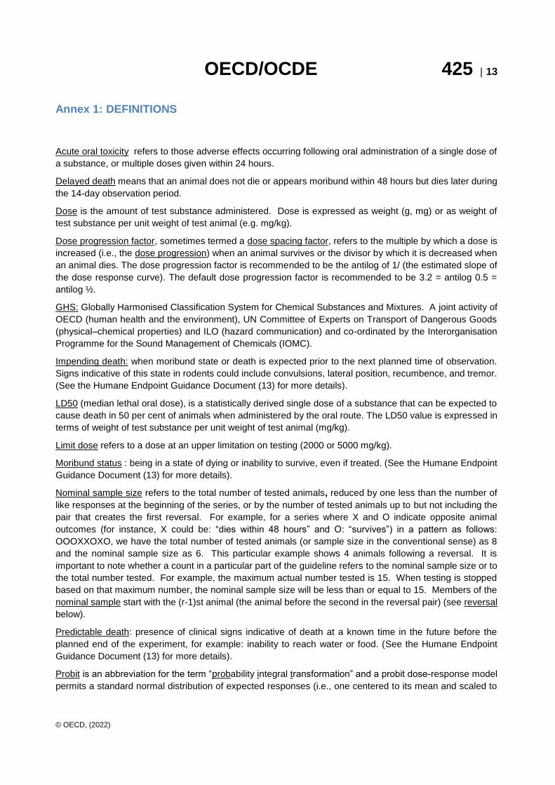
Annex 1: DEFINITIONS

Acute oral toxicity refers to those adverse effects occurring following oral administration of a single dose of

a substance, or multiple doses given within 24 hours.

Delayed death means that an animal does not die or appears moribund within 48 hours but dies later during

the 14-day observation period.

Dose is the amount of test substance administered. Dose is expressed as weight (g, mg) or as weight of

test substance per unit weight of test animal (e.g. mg/kg).

Dose progression factor, sometimes termed a dose spacing factor, refers to the multiple by which a dose is

increased (i.e., the dose progression) when an animal survives or the divisor by which it is decreased when

an animal dies. The dose progression factor is recommended to be the antilog of 1/ (the estimated slope of

the dose response curve). The default dose progression factor is recommended to be 3.2 = antilog 0.5 =

antilog ½.

GHS: Globally Harmonised Classification System for Chemical Substances and Mixtures. A joint activity of

OECD (human health and the environment), UN Committee of Experts on Transport of Dangerous Goods

(physical–chemical properties) and ILO (hazard communication) and co-ordinated by the Interorganisation

Programme for the Sound Management of Chemicals (IOMC).

Impending death: when moribund state or death is expected prior to the next planned time of observation.

Signs indicative of this state in rodents could include convulsions, lateral position, recumbence, and tremor.

(See the Humane Endpoint Guidance Document (13) for more details).

LD50 (median lethal oral dose), is a statistically derived single dose of a substance that can be expected to

cause death in 50 per cent of animals when administered by the oral route. The LD50 value is expressed in

terms of weight of test substance per unit weight of test animal (mg/kg).

Limit dose refers to a dose at an upper limitation on testing (2000 or 5000 mg/kg).

Moribund status : being in a state of dying or inability to survive, even if treated. (See the Humane Endpoint

Guidance Document (13) for more details).

Nominal sample size refers to the total number of tested animals, reduced by one less than the number of

like responses at the beginning of the series, or by the number of tested animals up to but not including the

pair that creates the first reversal. For example, for a series where X and O indicate opposite animal

outcomes (for instance, X could be: “dies within 48 hours” and O: “survives”) in a pattern as follows:

OOOXXOXO, we have the total number of tested animals (or sample size in the conventional sense) as 8

and the nominal sample size as 6. This particular example shows 4 animals following a reversal. It is

important to note whether a count in a particular part of the guideline refers to the nominal sample size or to

the total number tested. For example, the maximum actual number tested is 15. When testing is stopped

based on that maximum number, the nominal sample size will be less than or equal to 15. Members of the

nominal sample start with the (r-1)st animal (the animal before the second in the reversal pair) (see reversal

below).

Predictable death: presence of clinical signs indicative of death at a known time in the future before the

planned end of the experiment, for example: inability to reach water or food. (See the Humane Endpoint

Guidance Document (13) for more details).

Probit is an abbreviation for the term “probability integral transformation” and a probit dose-response model

permits a standard normal distribution of expected responses (i.e., one centered to its mean and scaled to

OECD/OCDE 425 14

© OECD, (2022)

its standard deviation, ) to doses (typically in a logarithmic scale) to be analyzed as if it were a straight line

with slope the reciprocal of . A standard normal lethality distribution is symmetric; hence, its mean is also

its true LD50 or median response.

Reversal is a situation where nonresponse is observed at some dose, and a response is observed at the

next dose tested, or vice versa (i.e., response followed by nonresponse). Thus, a reversal is created by a

pair of responses. The first such pair occurs at animals numbered r-1 and r.

is the standard deviation of a log normal curve describing the range of tolerances of test subjects to the

chemical (where a subject is expected capable of responding if the chemical dose exceeds the subject’s

tolerance). The estimated provides an estimate of the variation among test animals in response to a full

range of doses.

See slope and probit.

Slope (of the dose-response curve) is a value related to the angle at which the dose response curve rises

from the dose axis. In the case of probit analysis, when responses are analyzed on a probit scale against

dose on a log scale this curve will be a straight line and the slope is the reciprocal of , the standard deviation

of the underlying test subject tolerances, which are assumed to be normally distributed. See probit and .

Stopping rule is used in this guideline synonymously with 1) a specific stopping criterion and 2) the collection

of all criteria determining when a testing sequence terminates. In particular, for the main test, stopping rule

is used in paragraph 7 as a shorthand for the criterion that relies on comparison of ratios to a critical value.

OECD/OCDE 425 15

© OECD, (2022)

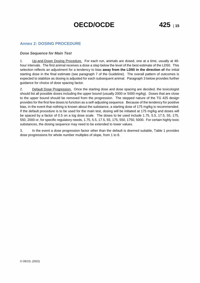
Annex 2: DOSING PROCEDURE

Dose Sequence for Main Test

1. Up-and-Down Dosing Procedure. For each run, animals are dosed, one at a time, usually at 48-

hour intervals. The first animal receives a dose a step below the level of the best estimate of the LD50. This

selection reflects an adjustment for a tendency to bias away from the LD50 in the direction of the initial

starting dose in the final estimate (see paragraph 7 of the Guideline). The overall pattern of outcomes is

expected to stabilize as dosing is adjusted for each subsequent animal. Paragraph 3 below provides further

guidance for choice of dose spacing factor.

2. Default Dose Progression. Once the starting dose and dose spacing are decided, the toxicologist

should list all possible doses including the upper bound (usually 2000 or 5000 mg/kg). Doses that are close

to the upper bound should be removed from the progression. The stepped nature of the TG 425 design

provides for the first few doses to function as a self-adjusting sequence. Because of the tendency for positive

bias, in the event that nothing is known about the substance, a starting dose of 175 mg/kg is recommended.

If the default procedure is to be used for the main test, dosing will be initiated at 175 mg/kg and doses will

be spaced by a factor of 0.5 on a log dose scale. The doses to be used include 1.75, 5.5, 17.5, 55, 175,

550, 2000 or, for specific regulatory needs, 1.75, 5.5, 17.5, 55, 175, 550, 1750, 5000. For certain highly toxic

substances, the dosing sequence may need to be extended to lower values.

3. In the event a dose progression factor other than the default is deemed suitable, Table 1 provides

dose progressions for whole number multiples of slope, from 1 to 8.

OECD/OCDE 425 16

© OECD, (2022)

Table 1 Dose Progressions for OECD Test Guideline 425. Choose a Slope and Read Down the Column.All doses in mg/kg bw

Slope =

1

2

3

4

5

6

7

8

0.175*

0.175*

0.175*

0.175*

0.175*

0.175*

0.175*

0.175*

0.24

0.23

0.275

0.26

0.31

0.34

0.31

0.375

0.375

0.41

0.44

0.47

0.55

0.55

0.55

0.55

0.69

0.65

0.73

0.81

0.82

0.99

0.91

0.97

1.09

1.2

1.26

1.29

1.75

1.75

1.75

1.75

1.75

1.75

1.75

1.75

2.4

2.3

2.75

2.6

3.1

3.4

3.1

3.75

3.75

4.4

4.1

4.7

5.5

5.5

5.5

5.5

6.9

6.5

7.3

8.1

8.2

9.9

9.1

9.7

10.9

12

12.6

12.9

17.5

17.5

17.5

17.5

17.5

17.5

17.5

17.5

24

23

27.5

26

31

34

31

OECD/OCDE 425 17

© OECD, (2022)

Table 1 continued

Slope =

1

2

3

4

5

6

7

8

37.5

37.5

44

41

47

55

55

55

55

65

69

73

81

82

99

91

97

109

120

126

129

175

175

175

175

175

175

175

175

240

230

275

260

310

340

310

375

375

440

410

470

550

550

550

550

650

690

730

810

820

990

910

970

1090

1200

1260

1290

1750

1750

1750

1750

1750

1750

1750

1750

2400

2300

2750

2600

3100

3100

3750

3400

4100

5000

5000

5000

5000

5000

5000

5000

5000

* If lower doses are needed, continue progressions to a lower dose

OECD/OCDE 425 18

© OECD, (2022)

Annex 3: COMPUTATIONS FOR THE LIKELIHOOD-RATIO STOPPING RULE

1. As described in Guideline paragraph 33, the main test may be completed on the basis of the first of

three stopping criteria to occur. In any case, even if none of the stopping criteria is satisfied, dosing would

stop when 15 animals are dosed. Tables 2-5 illustrate examples where testing has started with no

information, so the recommended default starting value, 175 mg/kg, and the recommended default dose

progression factor, 3.2 or one half log, have been used. Please note the formatting of these tables is only

illustrative.

2. Table 2 shows how the main test would stop if 3 animals have survived at the limit dose of 2000

mg/kg; Table 3 shows a similar situation when the limit dose of 5000 mg/kg is used. (These illustrate

situations where a Limit Test was not thought appropriate a priori.) Table 4 shows how a particular sequence

of 5 reversals in 6 tested animals could occur and allow test completion. Finally, Table 5 illustrates a situation

where neither criterion (a) nor criterion (b) has been met, a reversal of response has occurred followed by 4

tested animals, and, consequently, criterion (c) must be evaluated as well.

3. Criterion (c) calls for a likelihood-ratio stopping rule to be evaluated after testing each animal, starting

with the fourth tested following the reversal. Three "measures of test progress" are calculated. Technically,

these measures of progress are likelihoods, as recommended for the maximum-likelihood estimation of the

LD50. The procedure is closely related to calculation of a confidence interval by a likelihood-based

procedure.

4. The basis of the procedure is that when enough data have been collected, a point estimate of the

LD50 should be more strongly supported than values above and below the point estimate, where statistical

support is quantified using likelihood. Therefore three likelihood values are calculated: a likelihood at an

LD50 point estimate (called the rough estimate or dose-averaging estimate in the example), a likelihood at

a value below the point estimate, and a likelihood at a value above the point estimate. Specifically, the low

value is taken to be the point estimate divided by 2.5 and the high value is taken to be the point estimate

multiplied by 2.5.

5. The likelihood values are compared by calculating ratios of likelihoods, and then determining

whether these likelihood-ratios (LR) exceed a critical value. Testing stops when the ratio of the likelihood

for the point estimate exceeds each of the other likelihoods by a factor of 2.5, which is taken to indicate

relatively strong statistical support for the point estimate. Therefore two likelihood-ratios (LRs) are

calculated, a ratio of likelihoods for the point estimate and the point estimate divided by 2.5, and a ratio for

the point estimate and the estimate times 2.5.

6. The LD50 calculations alone are easily performed in any spreadsheet with normal probability

functions. The calculations are illustrated in Table 5 in this Annex 3 which is structured to imitate spreadsheet

implementation. The computation steps are illustrated using an example where the upper limit dose is 5000

mg/kg, but the computational steps are carried out in the same fashion when the upper boundary dose is

2000 mg/kg. Alternatively, self-contained software, that provides animal data entry grids and incorporates

the necessary formulas for LD50 estimation and confidence interval computation, is available for direct

downloading from the OECD and US EPA web sites. Table 6 shows a screen image from this software.

Hypothetical example using an upper limit dose of 5000 mg/kg (Table 5)

7. In the hypothetical example utilizing an upper boundary dose of 5000 mg/kg, the LR stopping

criterion was met after nine animals had been tested. The first “reversal” occurred with the 3rd animal tested.

OECD/OCDE 425 19

© OECD, (2022)

The LR stopping criterion is checked when four animals have been tested following the reversal. In this

example, the fourth animal tested following the reversal is the seventh animal actually tested. Therefore, for

this example, the spreadsheet calculations are only needed after the seventh animal had been tested and

the data could be entered at that time. Subsequently, the LR stopping criterion would have been checked

after testing the seventh animal, the eighth animal, and the ninth. The LR stopping criterion is first satisfied

after the ninth animal is tested in this example.

A. Enter the dose-response information animal by animal.

Column 1. Steps are numbered 1-15. No more than 15 animals may be tested.

Column 2. Place an I in this column as each animal is tested.

Column 3. Enter the dose received by the ith animal.

Column 4. Indicate whether the animal responded (shown by an X) or did not respond (shown by an

O).

B. The nominal and actual sample sizes.

8. The nominal sample consists of the two animals that represent the first reversal (here the second

and third animals), plus all animals tested subsequently. Here, Column 5 indicates whether or not a given

animal is included in the nominal sample.

The nominal sample size (nominal n) appears in Row 16. This is the number of animals in the nominal

sample. In the example, nominal n is 8.

The actual number tested appears in Row 17.

C. Rough estimate of the LD50.

9. The geometric mean of doses for the animals in the current nominal sample is used as a rough

estimate of the LD50 from which to gauge progress. In the table, this is called the “dose-averaging

estimator.” It is updated with each animal tested. This average is restricted to the nominal sample in order

to allow for a poor choice of initial test dose, which could generate either an initial string of responses or an

initial string of non-responses. (However, the results for all animals are used in the likelihood calculations

for final LD50 calculation below.) Recall that the geometric mean of n numbers is the product of the n

numbers, raised to a power of 1/n.

The dose-averaging estimate appears in Row 18 (e.g., (175 * 550 * ... * 1750 )1/8 = 1292.78).

Row 19 shows the logarithm (base 10) of the value in Row 18 (e.g., log10 1292.8 = 3.112).

D. Likelihood for the rough LD50 estimate.

OECD/OCDE 425 20

© OECD, (2022)

10. Likelihood is a statistical measure of how strongly the data support an estimate of the LD50 or other

parameter. Ratios of likelihood values can be used to compare how well the data support different estimates

of the LD50.

11. In column 8 calculate the likelihood for Step C’s rough LD50 estimate. The likelihood (Row 21) is

the product of likelihood contributions for individual animals (see Guideline paragraph 41). The likelihood

contribution for the ith animal is denoted Li.

12. In column 7 enter the estimate of the probability of response at dose di, denoted Pi. Pi is calculated

from a dose-response curve. Note that the parameters of a probit dose-response curve are the slope and

the LD50, so values are needed for each of those parameters. For the LD50 the dose-averaging estimate

from Row 18 is used. For the slope in this example the default value of 2 is used. The following steps may

be used to calculate the response probability Pi.

1. Calculate the base-10 log of dose di (Column 6).

2. For each animal calculate the z-score, denoted Zi (not shown in the table), using the formulae

= 1 / slope,

Zi = ( log10( di ) - log10( LD50 ) ) /

For example, for the first animal (Row 1),

= 1 / 2

Z1 = ( 2.243 - 3.112 ) / 0.500 = -1.738

3. For the ith dose the estimated response probability is

Pi = F( Zi )

where F denotes the cumulative distribution function for the standard normal distribution (i.e., the normal

distribution with mean 0 and variance 1).

For example (Row 1),

P 1 = F( -1.738 ) = 0.0412

The function F (or something very close) is ordinarily what is given for the normal distribution in statistical

tables, but the function is also widely available as a spreadsheet function. It is available under different

names, for example the @NORMAL function of Lotus 1-2-3 (1) and the @NORMDIST function in Excel (2).

To confirm that you have used correctly the function available in your software, you may wish to verify familiar

values such as F(1.96) 0.975 or F(1.64) 0.95.

13. Column 8. Calculate the natural log of the likelihood contribution (ln( Li )). Li is simply the probability

of the response that actually was observed for the ith animal:

OECD/OCDE 425 21

© OECD, (2022)

responding animals: ln( Li ) = ln ( Pi )

non-responding animals: ln( Li ) = ln( 1 - Pi )

Note that here the natural logarithm (ln) is used, whereas elsewhere the base-10 (common) logarithm was

used. These choices are what are ordinarily expected in a given context.

The steps above are performed for each animal. Finally:

Row 20: Sum the log-likelihood contributions in Column 8.

Row 21: Calculate the likelihood by applying the exp function applied to the log-likelihood

value in Row 20 (e.g., exp(-3.389) = e-3.389 = 0.0337).

E. Calculate likelihoods for two dose values above and below the rough estimate.

14. If the data permit a precise estimate, then one expects the likelihood should be high if the estimate

is a reasonable estimate of the LD50, relative to likelihoods for values distant from this estimate. Compare

the likelihood for the dose-averaging estimate (1292.8, Row 18) to values differing by a factor of 2.5 from

that value (i.e., to 1292.8*2.5 and 1292.8/2.5). The calculations (displayed in Columns 9-12) are carried out

in a fashion similar to those described above, except that the values 517.1 (=1292.8/2.5) and 3232.0

(=1292.8*2.5) have been used for the LD50, instead of 1292.8. The likelihoods and log-likelihoods are

displayed in Rows 20-21.

F. Calculate likelihood-ratios.

15. The three likelihood values (Row 21) are used to calculate two likelihood-ratios (Row 22). A

likelihood-ratio is used to compare the statistical support for the estimate of 1292.8 to the support for each

of the other values, 517.1 and 3232.0. The two likelihood-ratios are therefore:

LR1 = [likelihood of 1292.8] / [likelihood of 517.1]

= 0.0337 / 0.0080

= 4.21

and

LR2 = [likelihood of 1292.8] / [likelihood of 3232.0]

= 0.0337 / 0.0098

= 3.44

G. Determine if the likelihood-ratios exceed the critical value.

16. High likelihood-ratios are taken to indicate relatively high support for the point estimate of the LD50.

Both of the likelihood-ratios calculated in Step F (4.21 and 3.44) exceed the critical likelihood-ratio, which is

2.5. Therefore the LR stopping criterion is satisfied and testing stops. This is indicated by a TRUE in Row

24 and a note at the top of the example spreadsheet that the LR criterion is met.

OECD/OCDE 425 22

© OECD, (2022)

LITERATURE

(1) Lotus Development Corporation (1999). Lotus 1-2-3. Version 9.5, Millenium Edition. Cambridge, MA,

USA.

(2) Microsoft Corporation (1985-1997). Microsoft Excel Version 5.0 or later. Seattle, WA, USA.

OECD/OCDE 425 23

For Official Use

OECD/OCDE 425 24

For Official Use

OECD/OCDE 425 25

For Official Use

OECD/OCDE 425 26

For Official Use

OECD/OCDE 425 27

For Official Use

Table 6. Example of stopping criterion (c) from Self-contained Software for OECD Guideline 425

OECD/OCDE 425 28

For Official Use

Annex 4: CRITERIA FOR CLASSIFICATION OF TEST SUBSTANCES WITH

EXPECTED LD50 VALUES EXCEEDING 2000 MG/KG WITHOUT THE NEED FOR

TESTING

1. Criteria for hazard Category 5 are intended to enable the identification of test substances which

are of relatively low acute toxicity hazard but which, under certain circumstances may present a danger to

vulnerable populations. These substances are anticipated to have an oral or dermal LD50 in the range of

2000-5000 mg/kg or equivalent doses for other routes. Test substances could be classified in the hazard

category defined by: 2000 mg/kg<LD50<5000 mg/kg (Category 5 in the GHS) in the following cases:

a) if reliable evidence is already available that indicates the LD50 to be in the range of

Category 5 values; or other animal studies or toxic effects in humans indicate a concern

for human health of an acute nature.

b) through extrapolation, estimation or measurement of data if assignment to a more

hazardous category is not warranted, and

reliable information is available indicating significant toxic effects in humans, or

any mortality is observed when tested up to Category 4 values by the oral route, or

where expert judgement confirms significant clinical signs of toxicity, when tested

up to Category 4 values, except for diarrhoea, piloerection or an ungroomed

appearance, or

where expert judgement confirms reliable information indicating the potential for

significant acute effect from the other animal studies.

TESTING AT DOSES ABOVE 2000 MG/KG

2. Recognising the need to protect animal welfare, testing in animals in Category 5 ranges is

discouraged and should only be considered when there is a strong likelihood that results of such a test

would have a direct relevance for protecting human health.