ARTICLE IN PRESS

1352-2310/$ - se

doi:10.1016/j.at

�Correspondfax: +30231 09

E-mail addr

Atmospheric Environment 42 (2008) 1777–1789

www.elsevier.com/locate/atmosenv

Development of a computational system for estimating biogenicNMVOCs emissions based on GIS technology

Panagiotis Symeonidisa, Anastasia Poupkoub,�, Anthia Gkantoub,Dimitrios Melasb, Ozan Devrim Yayc, Evangelia Pouspourikab, Dimitrios Balisb

aDRAXIS Environmental Technologies, 63 Mitropoleos Street, 54623 Thessaloniki, GreecebLaboratory of Atmospheric Physics, Department of Physics, Aristotle University of Thessaloniki, P.O. Box 149, 54124 Thessaloniki, Greece

cDepartment of Environmental Engineering, Anadolu University, Eskis-ehir, Turkey

Received 9 January 2007; received in revised form 9 November 2007; accepted 13 November 2007

Abstract

A computational system was developed that can be used for the compilation of spatially and temporally resolved

biogenic non-methane volatile organic compounds emission inventories. A Geographic Information System was used to

integrate a variety of input data including: satellite land use data, land-use specific emission potentials and foliar biomass

densities, temperature and solar radiation data. The computational system was implemented focusing on the Balkan

Peninsula and a biogenic isoprene, monoterpenes and other volatile organic compounds emission inventory was produced.

The inventory has 1 km spatial resolution and is driven by mean climatology. The annual total biogenic non-methane

volatile organic compounds (NMVOCs) emissions over the study area are estimated to be 3769.2Gg, composed of 36.1%

isoprene, 26.8% monoterpenes and 37.1% other volatile organic compounds (OVOCs). Approximately, 94% of annual

isoprene emissions are produced from May to September, while this percentage is lower for monoterpenes and OVOCs

(70% and 85%, respectively). Vegetation is a strong source of NMVOCs emissions in the study domain. On a country

basis, for most of the countries studied, annual biogenic emissions represent a large share of the annual total NMVOCs

emissions ranging from 70% to 80%.

r 2007 Elsevier Ltd. All rights reserved.

Keywords: Biogenic emissions; NMVOCs; Emission inventory; GIS

1. Introduction

A vast variety and significant quantities of non-methane volatile organic compounds (NMVOCs)are produced and emitted into the atmosphere byvegetation (Seinfeld and Pandis, 1998). Biogenic

e front matter r 2007 Elsevier Ltd. All rights reserved

mosenv.2007.11.019

ing author. Tel.: +30231 099 8009;

9 8090.

ess: poupkou@auth.gr (A. Poupkou).

NMVOCs play a significant role in determiningglobal tropospheric chemistry and regional andlocal photochemical oxidant formation (Geronet al., 1994). They react with hydroxyl radical,ozone and nitrate radical in the atmosphere,resulting in the formation of carbon monoxideand organic species that can enhance concentrationsof ozone and other oxidants in environments rich innitrogen oxides (Naik et al., 2004). Surface fluxes ofthese compounds are also of interest because they

.

ARTICLE IN PRESSP. Symeonidis et al. / Atmospheric Environment 42 (2008) 1777–17891778

have a key role in the global carbon cycle andglobal climate as most of them are oxidised tocarbon dioxide in the atmosphere and determinethe growth rate of atmospheric methane concentra-tions (Guenther et al., 1995). Consequently, acritical element in the description of atmosphericchemistry is an accurate and of high spatial andtemporal resolution emission inventory of biogenicNMVOCs.

Biogenic NMVOCs emissions are grouped intothree categories: isoprene (C5H8), monoterpenes(C10Hx) and other volatile organic compounds(OVOCs) (CxHyOz). Isoprene and monoterpenesemissions are the most analytically studied.

Isoprene is generally the compound of mostimportance for ozone studies and it is useful toinventory this compound specifically. It is typicallyemitted by deciduous trees in the presence ofPhotosynthetically Active Radiation, exhibiting astrong emission increase as temperature increases.Isoprene emissions appear to be a species-dependentby-product of photosynthesis, photorespiration, orboth (Seinfeld and Pandis, 1998). Singsaas et al.(1997) indicate that isoprene protects plants againstrapid and frequent high temperature episodes.

Monoterpenes are typically emitted by conifers.Monoterpenes have been suggested to have a numberof ecological roles such as defence against herbivores,attraction of pollinating insects, pheromonal produc-tion and plant allelopathy (Harborne, 1991; Guentheret al., 1993). Monoterpenes emissions are usuallytemperature dependent. However, some evergreenoaks and Norway spruce exhibit both temperatureand light dependency of monoterpenes emissions(Kesselmeier et al., 1996; Seufert et al., 1997).

OVOCs consist of a wide variety of compounds(alcohols, ketones, esters, ethers, aldehydes, alkenesand alkanes) and little is known about thequantitative emissions of individual species andtheir role in atmospheric chemistry. For that reason,they are studied as a separate category with a highlevel of uncertainty and the emissions estimationresults should be considered mainly as informative.

Globally, anthropogenic NMVOCs emissionsamount to only 10% of the total biogenic NMVOCsemissions from forests (Muller, 1992; Piccot et al.,1992; Guenther et al., 1995). However, the Eur-opean scale anthropogenic and biogenic NMVOCsemissions have comparable magnitudes. BiogenicNMVOCs emissions are estimated at 14Tg yr�1

compared to man-made emissions of around24Tg yr�1 (Simpson et al., 1999).

This paper describes the development of acomputational system for estimating biogenicNMVOCs emissions based on Geographic Informa-tion System (GIS) technology. The computationalsystem was implemented for the compilation of aspatially and temporally resolved emission inven-tory for the Balkan Peninsula. The background ofthe employed methodology is provided in Section 2.The developed system and the input data integratedby the GIS used are described in Section 3. InSection 4, the spatially resolved isoprene, mono-terpenes and OVOCs biogenic emissions are pre-sented. In the same section, a comparison is shownbetween the total biogenic and anthropogenicNMVOCs emissions. In Section 5, the areas of datalimitations are indicated and the annual biogenicNMVOCs emissions on a country basis are com-pared with corresponding estimations of anothernatural emissions inventory in European scale.

2. Description of the mathematical model

For all types of vegetation, an appropriatemathematical model describing the emissions fluxon an hourly basis is that of Guenther et al. (1993):

Flux ðmgm�2 h�1Þ ¼ �Dg, (1)

where e is the emission potential (mg gdryweight foliage�1 h�1) for any particular speciesat a standard temperature Ts ¼ 303K and astandard Photosynthetically Active Radiation(PAR) flux ( ¼ 1000 mmol photons (400–700 nm)m�2 s�1), D is the foliar biomass density (g dryweight foliagem�2), and g is a unit less environ-mental correction factor representing the effects ofshort-term (e.g. hourly) temperature and solarradiation changes on emissions.

Light and temperature account for most of theobserved diurnal variation in biogenic emissions.There are two general models that can be used toreproduce NMVOCs emissions variation due tochanges in light and leaf temperature. The firstmodel is temperature and light dependent, while thesecond is dependent only on temperature.

2.1. Isoprene

Guenther et al. (1991, 1993) showed that to a verygood approximation, the short-term variations inemissions of isoprene could be described by theproduct of a light-dependent factor CLiso

and a

ARTICLE IN PRESSP. Symeonidis et al. / Atmospheric Environment 42 (2008) 1777–1789 1779

temperature-dependent factor CTiso:

giso ¼ CLisoCTiso

. (2)

The light-dependent factor is given by:

CLiso¼

acL1Lffiffiffiffiffiffiffiffiffiffiffiffiffiffiffiffiffiffi1þ a2L2

p , (3)

where a ¼ 0.0027 and cL1 ¼ 1.066 are empiricalconstants, and L is the PAR flux (mmol photons(400–700 nm)m�2 s�1).

The temperature dependence is described by:

CTiso¼

expðCT1ðT � T sÞ=RT sTÞ

1þ expðCT2ðT � TMÞ=RT sTÞ, (4)

where R is the gas constant ( ¼ 8.314 JK�1mol�1)and CT1 ¼ 95,000 Jmol�1, CT2 ¼ 230,000 Jmol�1

and TM ¼ 314K are empirical coefficients, basedupon measurements of three plant species: eucalyp-tus, aspen and velvet bean, which seem to be validfor a variety of different plant species. T is the leaftemperature (in K) and Ts ¼ 303K is the standardtemperature.

In the current study, a simple non-canopyapproach was followed which assumed that leaftemperature and PAR flux within the canopy wereidentical to ambient levels and that the use ofbranch-level emission potentials, which are typicallya factor of 1.75 smaller than leaf-level values(Guenther et al., 1994), accounted for the shadingeffects (Simpson et al., 1999).

2.2. Monoterpenes

The environmental correction factor for mono-terpenes emitted from most plants is parameterisedusing the following equation (Guenther et al., 1993):

gmts ¼ expðb� ðT � T sÞÞ, (5)

where b ¼ 0.09K�1 is an empirical coefficient basedon nonlinear regression analysis of numerousmeasurements present in the literature.

The light dependency of monoterpenes emittedfrom some vegetation species seems to be welldescribed by the isoprene algorithm (EMEP/COR-INAIR, 2002).

2.3. OVOCs

Since the environmental conditions controllingemissions of OVOCs are even less understood thanisoprene and monoterpenes and given the lack ofother information, OVOCs emissions are considered

temperature dependent and the use of Eq. (5) isrecommended for the estimation of their emissions(Guenther et al., 1994):

gOVOC ¼ gmts. (6)

3. Description of the computational system

The computational system developed allows thecalculation of isoprene, monoterpenes and OVOCsemissions from vegetation. More particularly, a GISwas used to integrate a variety of input dataincluding: (1) satellite land use data, (2) land-usespecific emission potentials and foliar biomassdensities, (3) temperature data and (4) solar radia-tion data, in order a spatially and temporallyresolved biogenic NMVOCs emission inventory tobe produced. The computational system flowdiagram is presented in Fig. 1. The computationalsystem was implemented focusing on the BalkanPeninsula. The biogenic NMVOCs emission inven-tory produced was driven by mean climatologysince detailed meteorological data for the timeperiod of a whole year were not available. Overthe study area, the typical diurnal variation ofbiogenic emissions was calculated for every monthof a year with 1 km spatial resolution. Daily,monthly and annual emission values were alsoestimated.

3.1. Land use data

The source of the land use information was theGlobal Land Cover Characteristics database(GLCC version 2) distributed by US GeologicalSurvey. The GLCC database is based on 1-kmAVHRR data spanning April 1992–March 1993updated by local contributions where possible. Thedataset used was the Eurasia Seasonal Land CoverRegions Legend which assigns each area of theEurasia’s surface to one of 253 different land useclasses. The Balkan Peninsula is covered by 169different land use classes emitting biogenicNMVOCs that are characterised by:

(1)

one vegetation species (e.g. pine woodland,wheat cropland) or

(2)

one ecosystem type (e.g. deciduous broadleafforest) or

(3)

a combination of vegetation species and/orecosystem types (e.g. oak woodland with grass-land).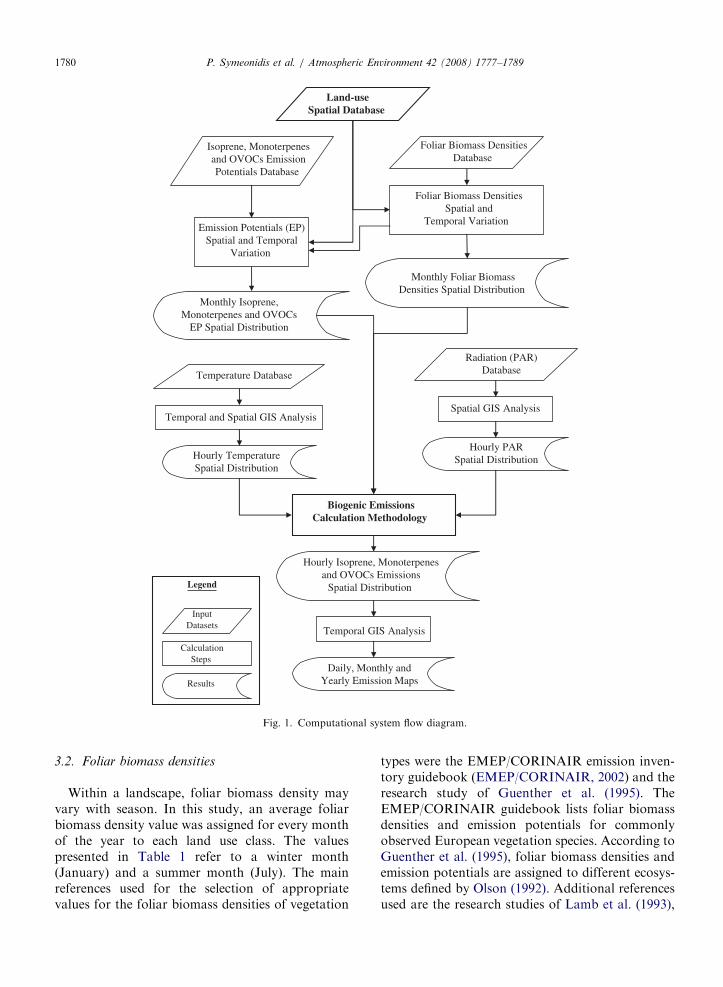

ARTICLE IN PRESS

Land-useSpatial Database

Foliar Biomass DensitiesDatabase

Temporal GIS Analysis

Isoprene, Monoterpenesand OVOCs EmissionPotentials Database

Emission Potentials (EP)Spatial and Temporal

Variation

Foliar Biomass DensitiesSpatial and

Temporal Variation

Monthly Foliar BiomassDensities Spatial Distribution

Monthly Isoprene,Monoterpenes and OVOCs

EP Spatial Distribution

Temperature Database

Temporal and Spatial GIS Analysis

Hourly TemperatureSpatial Distribution

Biogenic EmissionsCalculation Methodology

Hourly Isoprene, Monoterpenesand OVOCs Emissions

Spatial Distribution

Daily, Monthly andYearly Emission Maps

InputDatasets

Legend

CalculationSteps

Results

Hourly PARSpatial Distribution

Spatial GIS Analysis

Radiation (PAR)Database

Fig. 1. Computational system flow diagram.

P. Symeonidis et al. / Atmospheric Environment 42 (2008) 1777–17891780

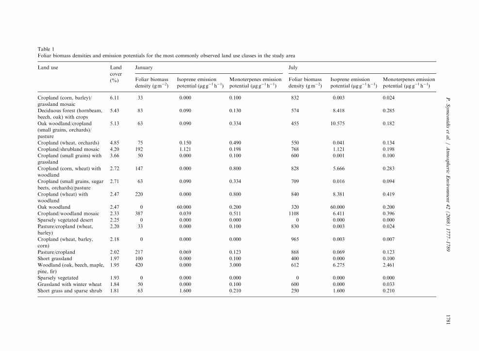
3.2. Foliar biomass densities

Within a landscape, foliar biomass density mayvary with season. In this study, an average foliarbiomass density value was assigned for every monthof the year to each land use class. The valuespresented in Table 1 refer to a winter month(January) and a summer month (July). The mainreferences used for the selection of appropriatevalues for the foliar biomass densities of vegetation

types were the EMEP/CORINAIR emission inven-tory guidebook (EMEP/CORINAIR, 2002) and theresearch study of Guenther et al. (1995). TheEMEP/CORINAIR guidebook lists foliar biomassdensities and emission potentials for commonlyobserved European vegetation species. According toGuenther et al. (1995), foliar biomass densities andemission potentials are assigned to different ecosys-tems defined by Olson (1992). Additional referencesused are the research studies of Lamb et al. (1993),

ARTIC

LEIN

PRES

S

Table 1

Foliar biomass densities and emission potentials for the most commonly observed land use classes in the study area

Land use Land

cover

(%)

January July

Foliar biomass

density (gm�2)

Isoprene emission

potential (mg g�1 h�1)Monoterpenes emission

potential (mg g�1 h�1)Foliar biomass

density (gm�2)

Isoprene emission

potential (mg g�1 h�1)Monoterpenes emission

potential (mg g�1 h�1)

Cropland (corn, barley)/

grassland mosaic

6.11 33 0.000 0.100 832 0.003 0.024

Deciduous forest (hornbeam,

beech, oak) with crops

5.43 83 0.090 0.130 574 8.418 0.285

Oak woodland/cropland

(small grains, orchards)/

pasture

5.13 63 0.090 0.334 455 10.575 0.182

Cropland (wheat, orchards) 4.85 75 0.150 0.490 550 0.041 0.134

Cropland/shrubland mosaic 4.20 192 1.121 0.198 768 1.121 0.198

Cropland (small grains) with

grassland

3.66 50 0.000 0.100 600 0.001 0.100

Cropland (corn, wheat) with

woodland

2.72 147 0.000 0.800 828 5.666 0.283

Cropland (small grains, sugar

beets, orchards)/pasture

2.71 63 0.090 0.334 709 0.016 0.094

Cropland (wheat) with

woodland

2.47 220 0.000 0.800 840 8.381 0.419

Oak woodland 2.47 0 60.000 0.200 320 60.000 0.200

Cropland/woodland mosaic 2.33 387 0.039 0.511 1108 6.411 0.396

Sparsely vegetated desert 2.25 0 0.000 0.000 0 0.000 0.000

Pasture/cropland (wheat,

barley)

2.20 33 0.000 0.100 830 0.003 0.024

Cropland (wheat, barley,

corn)

2.18 0 0.000 0.000 965 0.003 0.007

Pasture/cropland 2.02 217 0.069 0.123 868 0.069 0.123

Short grassland 1.97 100 0.000 0.100 400 0.000 0.100

Woodland (oak, beech, maple,

pine, fir)

1.95 420 0.000 3.000 612 6.275 2.461

Sparsely vegetated 1.93 0 0.000 0.000 0 0.000 0.000

Grassland with winter wheat 1.84 50 0.000 0.100 600 0.000 0.033

Short grass and sparse shrub 1.81 63 1.600 0.210 250 1.600 0.210

P.

Sy

meo

nid

iset

al.

/A

tmo

sph

ericE

nviro

nm

ent

42

(2

00

8)

17

77

–1

78

91781

ARTICLE IN PRESSP. Symeonidis et al. / Atmospheric Environment 42 (2008) 1777–17891782

Geron et al. (1994), Guenther et al. (1994), Leviset al. (2003) and Parra et al. (2004). When a land useclass was characterised by a combination ofdifferent vegetation types, it was assumed that themonthly average foliar biomass density was equal tothe mean value of the foliar biomass densities of allvegetation types within the land use class.

Corrective factors were used to describe theseasonal variation of the foliar biomass densitiesof vegetation species and ecosystems. The foliarbiomass densities of deciduous trees were consid-ered to be maximum from May to September,decreased by half during October, November andApril and had zero value during the remainingmonths of the year (Simeonidis et al., 1999).Landscapes characterised as mixed forests wereassumed to be composed of both deciduous andevergreen trees and the corrective factors used todescribe their foliar biomass decrease during theyear was 0.5 for January, February, March andDecember and 0.75 for April, October and Novem-ber. The foliar biomass density seasonal variation ofagricultural crops was based on their growingseason. The corrective factors used to describe thefoliar biomass decrease of orchards during the yearwere 0.5 for January, February, March, Novemberand December and 0.75 for April and October. Thefoliar biomass densities of landscapes characterisedas grasslands, shrublands or croplands (when aspecific crop was not explicitly quoted) wereconsidered to be maximum fromMay to September,decreased by half during March, April, October andNovember and during the rest of the year wereequal to 1/4 of their maximum value. Tundralandscapes were assumed to have foliar biomassdensity which was maximum from June to August,decreased by half during May and September andwas equal to 1/4 of its maximum value during theremaining months of the year.

3.3. Emission potentials

Two approaches were used in order to assignisoprene, monoterpenes and OVOCs emission po-tentials to each land use class:

(1)

The first approach was employed for land useclasses characterised by a combination ofvegetation types that were explicitly defined(e.g. oak woodland with grassland). In this case,an emission potential was assigned to eachvegetation type within the land use class and

the resulting emissions from each vegetationtype were aggregated. The land use-specificemission potential (e) was estimated based onthe following equation:

� ¼

Pi¼ni¼1ð�iDi=nÞPi¼n

i¼1ðDi=nÞ, (7)

where ei and Di are the emission potentials andthe foliar biomass densities of each vegetationtype within the land use class and n is thenumber of vegetation types within the land useclass.

(2)

The second approach was to assign an emissionpotential directly to the land use class. Thisapproach was effective for land use classes withvegetation species diversity that was not expli-citly specified (e.g. deciduous broadleaf forest).

Isoprene, monoterpenes and OVOCs emissionpotentials were assigned for every month of theyear to each land use class emitting biogenicNMVOCs based on the list of references presentedin Section 3.2 and accounting for the seasonalvariation of the foliar biomass densities of vegeta-tion species and ecosystems (Table 1). All vegetationspecies and ecosystems were assigned an OVOCsemission potential of 1.5 mg g�1 h�1 based on therecommendations of Guenther et al. (1994). Theisoprene algorithm was applied in order the lightdependency of monoterpenes emissions from ever-green oaks to be accounted for.

3.4. Temperature data

The temperature data used for the calculation ofthe environmental correction factors (Eqs. (4) and(5)) were derived from the CRU Global ClimateDataset of the IPCC Data Distribution Center.The dataset provided mean monthly climatic dataof maximum and minimum temperature valuesfor the 1961–1990 period having 0.51 latitude by0.51 longitude spatial resolution. The inversedistance interpolation method was applied, increas-ing the spatial resolution of the temperature data to10 km. A typical temperature diurnal variationwas reproduced assuming that temperature wasminimum around 6:00 ST, increasing linearly toreach the maximum value around 14:00 ST andthen decreasing linearly to reach the minimumvalue again.

ARTICLE IN PRESSP. Symeonidis et al. / Atmospheric Environment 42 (2008) 1777–1789 1783

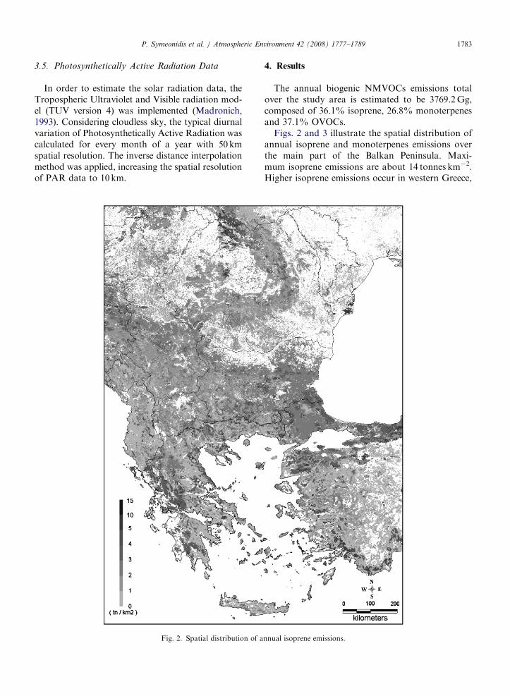
3.5. Photosynthetically Active Radiation Data

In order to estimate the solar radiation data, theTropospheric Ultraviolet and Visible radiation mod-el (TUV version 4) was implemented (Madronich,1993). Considering cloudless sky, the typical diurnalvariation of Photosynthetically Active Radiation wascalculated for every month of a year with 50kmspatial resolution. The inverse distance interpolationmethod was applied, increasing the spatial resolutionof PAR data to 10km.

Fig. 2. Spatial distribution of a

4. Results

The annual biogenic NMVOCs emissions totalover the study area is estimated to be 3769.2Gg,composed of 36.1% isoprene, 26.8% monoterpenesand 37.1% OVOCs.

Figs. 2 and 3 illustrate the spatial distribution ofannual isoprene and monoterpenes emissions overthe main part of the Balkan Peninsula. Maxi-mum isoprene emissions are about 14 tonnes km�2.Higher isoprene emissions occur in western Greece,

nnual isoprene emissions.

ARTICLE IN PRESS

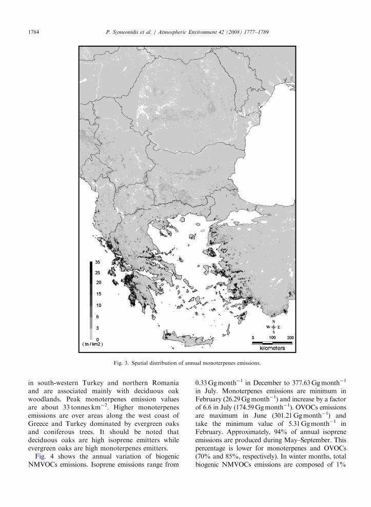
Fig. 3. Spatial distribution of annual monoterpenes emissions.

P. Symeonidis et al. / Atmospheric Environment 42 (2008) 1777–17891784

in south-western Turkey and northern Romaniaand are associated mainly with deciduous oakwoodlands. Peak monoterpenes emission valuesare about 33 tonnes km�2. Higher monoterpenesemissions are over areas along the west coast ofGreece and Turkey dominated by evergreen oaksand coniferous trees. It should be noted thatdeciduous oaks are high isoprene emitters whileevergreen oaks are high monoterpenes emitters.

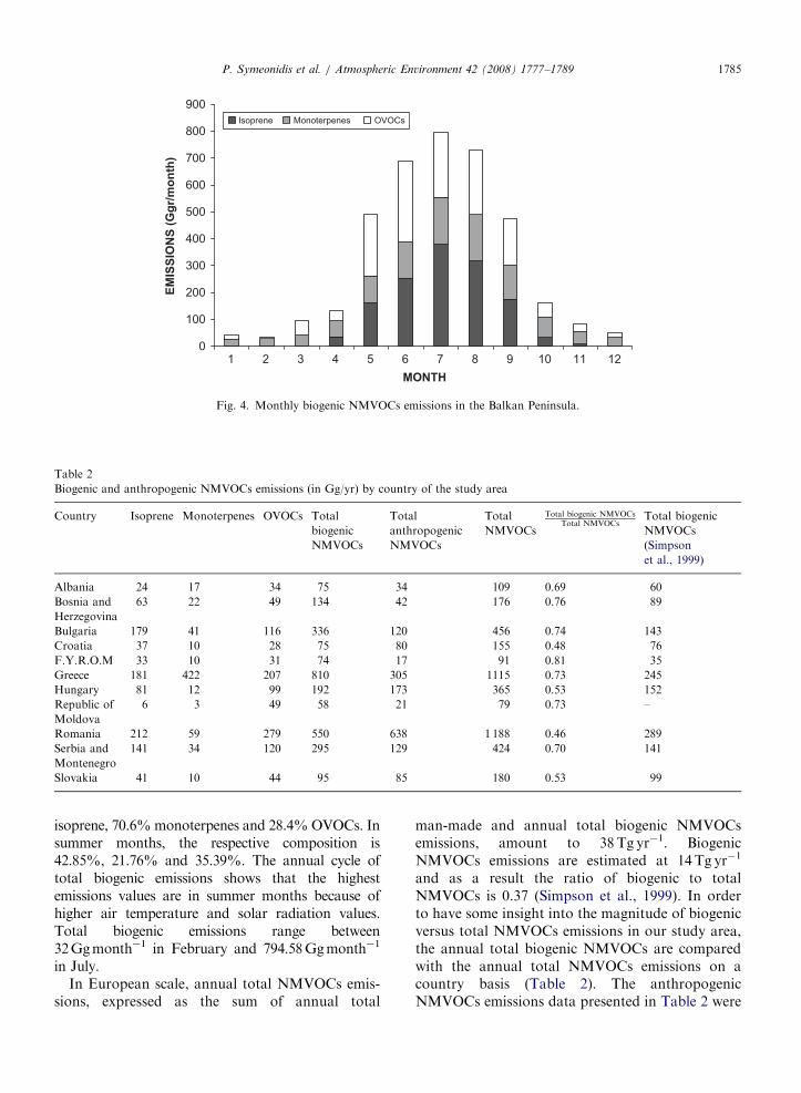
Fig. 4 shows the annual variation of biogenicNMVOCs emissions. Isoprene emissions range from

0.33Ggmonth�1 in December to 377.63Ggmonth�1

in July. Monoterpenes emissions are minimum inFebruary (26.29Ggmonth�1) and increase by a factorof 6.6 in July (174.59Ggmonth�1). OVOCs emissionsare maximum in June (301.21Ggmonth�1) andtake the minimum value of 5.31Ggmonth�1 inFebruary. Approximately, 94% of annual isopreneemissions are produced during May–September. Thispercentage is lower for monoterpenes and OVOCs(70% and 85%, respectively). In winter months, totalbiogenic NMVOCs emissions are composed of 1%

ARTICLE IN PRESS

0

100

200

300

400

500

600

700

800

900

1 3 7 10 11 12

EM

ISS

ION

S (

Gg

r/m

on

th)

Isoprene Monoterpenes OVOCs

MONTH

2 4 5 6 8 9

Fig. 4. Monthly biogenic NMVOCs emissions in the Balkan Peninsula.

Table 2

Biogenic and anthropogenic NMVOCs emissions (in Gg/yr) by country of the study area

Country Isoprene Monoterpenes OVOCs Total

biogenic

NMVOCs

Total

anthropogenic

NMVOCs

Total

NMVOCs

Total biogenic NMVOCsTotal NMVOCs

Total biogenic

NMVOCs

(Simpson

et al., 1999)

Albania 24 17 34 75 34 109 0.69 60

Bosnia and

Herzegovina

63 22 49 134 42 176 0.76 89

Bulgaria 179 41 116 336 120 456 0.74 143

Croatia 37 10 28 75 80 155 0.48 76

F.Y.R.O.M 33 10 31 74 17 91 0.81 35

Greece 181 422 207 810 305 1115 0.73 245

Hungary 81 12 99 192 173 365 0.53 152

Republic of

Moldova

6 3 49 58 21 79 0.73 –

Romania 212 59 279 550 638 1 188 0.46 289

Serbia and

Montenegro

141 34 120 295 129 424 0.70 141

Slovakia 41 10 44 95 85 180 0.53 99

P. Symeonidis et al. / Atmospheric Environment 42 (2008) 1777–1789 1785

isoprene, 70.6%monoterpenes and 28.4%OVOCs. Insummer months, the respective composition is42.85%, 21.76% and 35.39%. The annual cycle oftotal biogenic emissions shows that the highestemissions values are in summer months because ofhigher air temperature and solar radiation values.Total biogenic emissions range between32Ggmonth�1 in February and 794.58Ggmonth�1

in July.In European scale, annual total NMVOCs emis-

sions, expressed as the sum of annual total

man-made and annual total biogenic NMVOCsemissions, amount to 38Tg yr�1. BiogenicNMVOCs emissions are estimated at 14Tg yr�1

and as a result the ratio of biogenic to totalNMVOCs is 0.37 (Simpson et al., 1999). In orderto have some insight into the magnitude of biogenicversus total NMVOCs emissions in our study area,the annual total biogenic NMVOCs are comparedwith the annual total NMVOCs emissions on acountry basis (Table 2). The anthropogenicNMVOCs emissions data presented in Table 2 were

ARTICLE IN PRESSP. Symeonidis et al. / Atmospheric Environment 42 (2008) 1777–17891786

derived from the emission database of EMEP andcorrespond to national annual emission totals forthe reference year 2000 that were estimated by theEMEP experts based on officially reported emis-sions that had been corrected and completed(Vestreng et al., 2004). For most of the countriesin the study area, the total biogenic to totalNMVOCs emissions ratio ranges from 0.69 to 0.81being almost two times higher than the respectiveratio in European scale. For these countries,NMVOCs emissions from anthropogenic sourcesrepresent a share of biogenic NMVOCs emissionsranging from 23% to 45%. For Croatia, Hungary,Romania and Slovakia, annual man made andbiogenic NMVOCs emissions are almost of thesame magnitude.

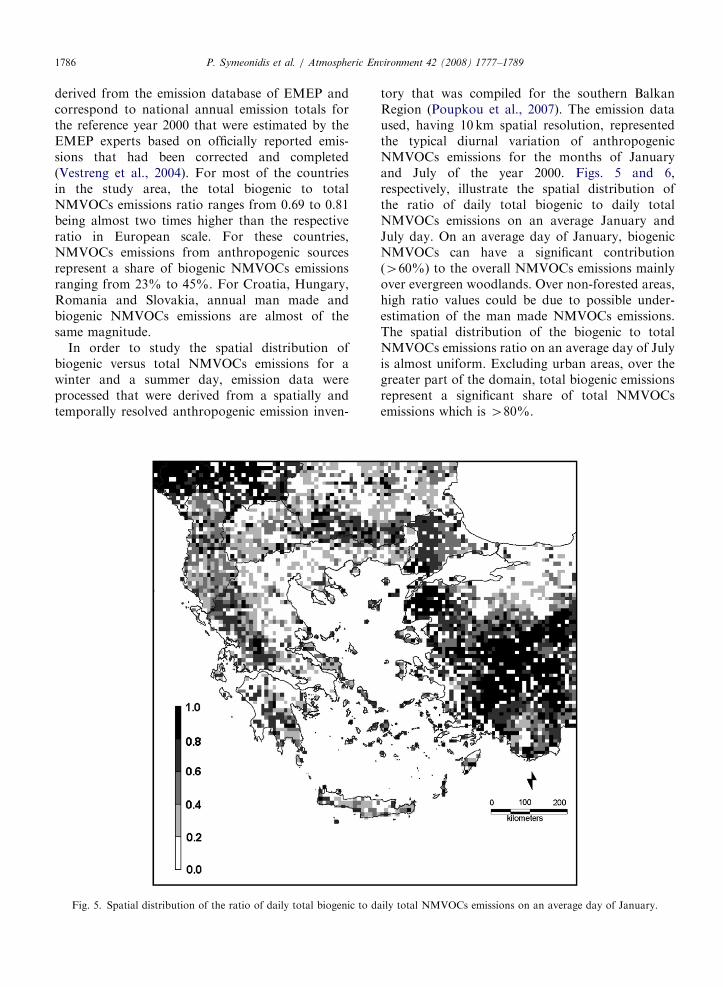
In order to study the spatial distribution ofbiogenic versus total NMVOCs emissions for awinter and a summer day, emission data wereprocessed that were derived from a spatially andtemporally resolved anthropogenic emission inven-

Fig. 5. Spatial distribution of the ratio of daily total biogenic to d

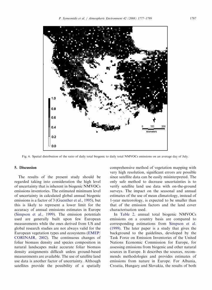
tory that was compiled for the southern BalkanRegion (Poupkou et al., 2007). The emission dataused, having 10 km spatial resolution, representedthe typical diurnal variation of anthropogenicNMVOCs emissions for the months of Januaryand July of the year 2000. Figs. 5 and 6,respectively, illustrate the spatial distribution ofthe ratio of daily total biogenic to daily totalNMVOCs emissions on an average January andJuly day. On an average day of January, biogenicNMVOCs can have a significant contribution(460%) to the overall NMVOCs emissions mainlyover evergreen woodlands. Over non-forested areas,high ratio values could be due to possible under-estimation of the man made NMVOCs emissions.The spatial distribution of the biogenic to totalNMVOCs emissions ratio on an average day of Julyis almost uniform. Excluding urban areas, over thegreater part of the domain, total biogenic emissionsrepresent a significant share of total NMVOCsemissions which is 480%.

aily total NMVOCs emissions on an average day of January.

ARTICLE IN PRESS

Fig. 6. Spatial distribution of the ratio of daily total biogenic to daily total NMVOCs emissions on an average day of July.

P. Symeonidis et al. / Atmospheric Environment 42 (2008) 1777–1789 1787

5. Discussion

The results of the present study should beregarded taking into consideration the high levelof uncertainty that is inherent in biogenic NMVOCsemissions inventories. The estimated minimum levelof uncertainty in calculated global annual biogenicemissions is a factor of 3 (Guenther et al., 1995), butthis is likely to represent a lower limit for theaccuracy of annual emissions estimates in Europe(Simpson et al., 1999). The emission potentialsused are generally built upon few Europeanmeasurements while the ones derived from US andglobal research studies are not always valid for theEuropean vegetation types and ecosystems (EMEP/CORINAIR, 2002). The continuous changes offoliar biomass density and species composition innatural landscapes make accurate foliar biomassdensity assignments difficult unless ground-basedmeasurements are available. The use of satellite landuse data is another factor of uncertainty. Althoughsatellites provide the possibility of a spatially

comprehensive method of vegetation mapping withvery high resolution, significant errors are possiblesince satellite data can be easily misinterpreted. Theonly safe method to decrease uncertainties is toverify satellite land use data with on-the-groundsurveys. The impact on the seasonal and annualestimates of the use of mean climatology, instead of1-year meteorology, is expected to be smaller thanthat of the emission factors and the land covercharacterisation used.

In Table 2, annual total biogenic NMVOCsemissions on a country basis are compared tocorresponding estimations from Simpson et al.(1999). The later paper is a study that gives thebackground to the guidelines, developed by theTask Force on Emission Inventories of the UnitedNations Economic Commission for Europe, forassessing emissions from biogenic and other naturalsources in Europe. It describes the sources, recom-mends methodologies and provides estimates ofemissions from nature in Europe. For Albania,Croatia, Hungary and Slovakia, the results of both

ARTICLE IN PRESSP. Symeonidis et al. / Atmospheric Environment 42 (2008) 1777–17891788

studies compare favourably. For the other coun-tries, the national emission estimates of the presentstudy are about two times higher than those ofSimpson et al. (1999). For Bosnia–Herzegovina andGreece, the overestimation is by a factor of 1.5 and3.3, respectively. Taking into consideration that theestimated minimum level of uncertainty in calcu-lated annual biogenic emissions is a factor of 3, theprevious comparison suggests that the results ofboth studies are in good agreement.

The comparison of biogenic with anthropogenicNMVOCs emissions should be regarded consideringthat uncertainties exist not only in calculatedbiogenic NMVOCs emissions but also when inven-torying anthropogenic NMVOCs. Anthropogenichydrocarbon emissions may be easily underesti-mated. Since anthropogenic hydrocarbons areemitted by both combustion and non-combustionsources, estimating hydrocarbons is less straightfor-ward than estimating anthropogenic emissions ofother pollutants (e.g. NOx) (Funk et al., 2001).

6. Conclusions

This study presents the development of a GIS-based computational system used for the estimationof biogenic NMVOCs emissions. The system wasimplemented focusing on the Balkan Peninsulaalthough a short extension of the developeddatabases of land use-specific emission potentialsand foliar biomass densities allows calculations inEuropean scale. A spatially and temporally resolvedbiogenic NMVOCs emission inventory was com-piled, driven by mean climatology. In the studydomain, the annual biogenic NMVOCs emissionstotal is estimated to be 3769.2Gg, composed of36.1% isoprene, 26.8% monoterpenes and 37.1%OVOCs. The annual cycle of total biogenic emis-sions depicts higher values during summer monthsin agreement with the expected influence on emis-sions of the air temperature and the solar radiation.Approximately, 94% of annual isoprene emissionsare produced during May–September, while thispercentage is lower for monoterpenes and OVOCs(70% and 85%, respectively).

For most Balkan countries, annual total biogenicNMVOCs emissions are in good agreement with aprevious biogenic emission inventory for Europe(Simpson et al., 1999) suggesting that the presentedemission inventory provides a reasonable estimationof NMVOCs emitted from vegetation in the BalkanPeninsula. Only for Greece, calculations differ by a

factor of 3 which is within the minimum reporteduncertainty levels.

Vegetation is a strong source of NMVOCsemissions in the study area. For most of thecountries, annual biogenic emissions represent alarge share of the annual total NMVOCs emissionsranging from 70% to 80%, while for the remainingones, man made and biogenic NMVOCs emissionsare almost of the same magnitude. The spatialdistribution of total biogenic versus total NMVOCsemissions reveals that on an average day of January,biogenic NMVOCs have a significant contribution(460%) to the overall NMVOCs emissions mainlyover evergreen woodlands. On an average day ofJuly, total NMVOCs emissions are dominated bybiogenic emissions over almost all non-urban areas.Given that isoprene is approximately a factor of 3more photochemically active than a weightedaverage of VOCs emitted by motor vehicle exhaust(Benjamin et al., 1997), the results of the presentstudy imply that a detailed biogenic NMVOCsemission inventory is a critical element of air qualitystudies focusing on the Balkan Peninsula.

Acknowledgements

The research study was partly financed by theEuropean Commission (research project ‘‘Globaland regional Earth-system Monitoring using Satel-lite and in-situ data’’, contract no.: 516099).

References

Benjamin, M., Sudol, M., Vorsatz, D., Winer, A., 1997. A

spatially and temporally resolved biogenic hydrocarbon

emissions inventory for the California South Coast Air Basin.

Atmospheric Environment 31, 3087–3100.

EMEP/CORINAIR, 2002. Atmospheric Emission Inventory Guide-

book, third ed., European Environment Agency, Copenhagen,

/http://reports.eea.europa.eu/EMEPCORINAIR3/en/page020.

htmlS.Funk, T.H., Chinkin, L.R., Roberts, P.T., Saeger, M., Mulligan,

S., Paramo Figueroa, V.H., Yarbrough, J., 2001. Compilation

and evaluation of a Paso del Norte emission inventory.

Science of the Total Environment 276, 135–151.

Geron, C., Guenther, A., Pierce, T., 1994. An improved model

for estimating emissions of volatile organic compounds from

forests in the Eastern United States. Journal of Geophysical

Research 99, 12773–12792.

Guenther, A.B., Monson, R.K., Fall, R., 1991. Isoprene and

monoterpene rate variability: observations with Eucalyptus

and emission rate algorithm development. Journal of

Geophysical Research 96, 10799–10808.

Guenther, A.B., Zimmerman, P.R., Harley, P.C., Monson, R.K.,

Fall, R., 1993. Isoprene and monoterpene rate variability:

ARTICLE IN PRESSP. Symeonidis et al. / Atmospheric Environment 42 (2008) 1777–1789 1789

model evaluations and sensitivity analyses. Journal of

Geophysical Research 98, 12609–12617.

Guenther, A., Zimmerman, P., Wildermuth, M., 1994. Natural

volatile organic compound emission rate estimates for US

woodland landscapes. Journal of Geophysical Research 28,

1197–1210.

Guenther, A., Hewitt, N., Erickson, D., Fall, R., Geron, C.,

Graedel, T., Harley, P., Klinger, L., Lerdau, M., McKay, W.,

Pierce, T., Scholes, B., Steinbrecher, R., Tallamraju, R.,

Taylor, J., Zimmerman, P., 1995. A global model of natural

volatile organic compound emissions. Journal of Geophysical

Research 100, 8873–8892.

Harborne, J.B., 1991. Recent advances in the ecological

chemistry of plant terpenoids. In: Harborne, J.B., Tomes-

Barberan, F.A. (Eds.), Ecological Chemistry and Biochem-

istry of Plant Terpenoids. Clarenden Press, Oxford, pp.

399–426.

Kesselmeier, J., Schafer, L., Ciccioli, P., Brancaleoni, E.,

Cecinato, A., Frattoni, M., Foster, P., Jacob, V., Denis, J.,

Fugit, J.L., Dutaur, L., Torres, L., 1996. Emission of

monoterpenes and isoprene from a Mediterranean oak species

Quercus ilex L. measured within the BEMA (Biogenic

emissions in the Mediterranean area) project. Atmospheric

Environment 30, 1841–1850.

Lamb, B., Gay, D., Westberg, H., Pierce, T., 1993. A biogenic

hydrocarbon emission inventory for the USA using a simple

forest canopy model. Atmospheric Environment 27, 1673–1690.

Levis, S., Wiedinmyer, C., Bonan, G.B., Guenther, A., 2003.

Simulating biogenic volatile organic compound emissions in

the Community Climate System Model. Journal of Geophy-

sical Research 108 (D21), 4659.

Madronich, S., 1993. UV radiation in the natural and perturbed

atmosphere. In: Tevini, M. (Ed.), Environmental Effects of UV

(Ultraviolet) Radiation. Lewis Publisher, Boca Raton, pp. 17–69.

Muller, J.-F., 1992. Geographical distribution and seasonal

variation of surface emissions and deposition velocities of

atmospheric trace gases. Journal of Geophysical Research 97,

3787–3804.

Naik, V., Delire, C., Wuebbles, D.J., 2004. Sensitivity of global

biogenic isoprenoid emissions to climate variability and

atmospheric CO2. Journal of Geophysical Research 109,

D06301.

Olson, J., 1992. World ecosystems (WE1.4): digital raster data on

a 10min geographic 1080� 2160 grid. In: Global Ecosystems

Database, Version 1.0: Disc A, NOAA National Geophysical

Data Center, Boulder, CO.

Parra, R., Gasso, S., Baldasano, J.M., 2004. Estimating the

biogenic emissions of non methane volatile organic com-

pounds from the North Western Mediterranean vegetation of

Catalonia, Spain. Science of the Total Environment 329,

241–259.

Piccot, S.D., Watson, J.J., Jones, J.W., 1992. A global inventory

of volatile organic compound emissions from anthropogenic

sources. Journal of Geophysical Research 97, 9897–9912.

Poupkou, A., Symeonidis, P., Ziomas, I., Melas, D., Markakis,

K., 2007. A spatially and temporally disaggregated anthro-

pogenic emission inventory in the southern Balkan Region.

Water, Air and Soil Pollution 185, 335–348.

Seinfeld, J., Pandis, S., 1998. Atmospheric Chemistry and

Physics. From Air Pollution to Climate Change. Wiley-

Interscience, pp. 82–85.

Seufert, G., Bartzis, J., Bomboi, T., Ciccioli, P., Cieslik, S., Dlugi, R.,

Foster, P., Hewitt, N., Kesselmeier, J., Kotzias, D., Lenz, R.,

Manes, F., Perez-Pastor, R., Steinbrecher, R., Torres, L.,

Valentini, R., Versino, B., 1997. The BEMA-project: an

overview of the Castelporziano experiments. Atmospheric

Environment 31 (S1), 5–17.

Simeonidis, P., Sanida, G., Ziomas, I., Kourtidis, K., 1999. An

estimation of the spatial and temporal distribution of biogenic

non-methane hydrocarbon emissions in Greece. Atmospheric

Environment 33, 3791–3801.

Simpson, D., Winiwarter, W., Borjesson, G., Cinderby, S.,

Ferreiro, A., Guenther, A., Hewitt, C.N., Janson, R., Khalil,

M.A.K., Owen, S., Pierce, T.E., Puxbaum, H., Shearer, M.,

Skiba, U., Steinbrecher, R., Tarrason, L., Oquist, M.G., 1999.

Inventorying emissions from nature in Europe. Journal of

Geophysical Research 104, 8113–8152.

Singsaas, E.L., Lerdau, M., Winter, K., Sharkey, T.D., 1997.

Isoprene increases thermotolerance of isoprene-emitting

species. Plant Physiology 115, 1413–1420.

Vestreng, V., Adams, M., Goodwin, J., 2004. Inventory Review

2004. Emission Data reported to CLRTAP and under the

NEC Directive. EMEP/EEA Joint Review Report, MSC-W

Technical Report 1/04.