DEVELOPMENT AND APPLICATION OF MASS TRANSFER CORRELATIONS FOR CO2

ABSORPTION IN PACKED COLUMNS

A Thesis

by

MATHEW T. DERICHSWEILER

Submitted to the Office of Graduate and Professional Studies ofTexas A&M University

in partial fulfillment of the requirements for the degree of

MASTER OF SCIENCE

Chair of Committee, Mahmoud El-HalwagiCommittee Members, Maria Barrufet

Kenneth HallHead of Department, Arul Jayaraman

December 2020

Major Subject: Chemical Engineering

Copyright 2020 Mathew T. Derichsweiler

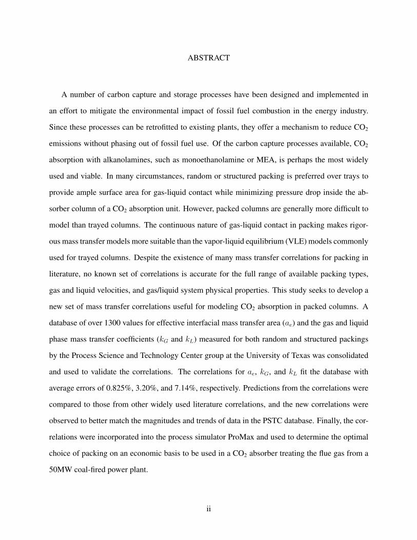
ABSTRACT

A number of carbon capture and storage processes have been designed and implemented in

an effort to mitigate the environmental impact of fossil fuel combustion in the energy industry.

Since these processes can be retrofitted to existing plants, they offer a mechanism to reduce CO2

emissions without phasing out of fossil fuel use. Of the carbon capture processes available, CO2

absorption with alkanolamines, such as monoethanolamine or MEA, is perhaps the most widely

used and viable. In many circumstances, random or structured packing is preferred over trays to

provide ample surface area for gas-liquid contact while minimizing pressure drop inside the ab-

sorber column of a CO2 absorption unit. However, packed columns are generally more difficult to

model than trayed columns. The continuous nature of gas-liquid contact in packing makes rigor-

ous mass transfer models more suitable than the vapor-liquid equilibrium (VLE) models commonly

used for trayed columns. Despite the existence of many mass transfer correlations for packing in

literature, no known set of correlations is accurate for the full range of available packing types,

gas and liquid velocities, and gas/liquid system physical properties. This study seeks to develop a

new set of mass transfer correlations useful for modeling CO2 absorption in packed columns. A

database of over 1300 values for effective interfacial mass transfer area (ae) and the gas and liquid

phase mass transfer coefficients (kG and kL) measured for both random and structured packings

by the Process Science and Technology Center group at the University of Texas was consolidated

and used to validate the correlations. The correlations for ae, kG, and kL fit the database with

average errors of 0.825%, 3.20%, and 7.14%, respectively. Predictions from the correlations were

compared to those from other widely used literature correlations, and the new correlations were

observed to better match the magnitudes and trends of data in the PSTC database. Finally, the cor-

relations were incorporated into the process simulator ProMax and used to determine the optimal

choice of packing on an economic basis to be used in a CO2 absorber treating the flue gas from a

50MW coal-fired power plant.

ii

ACKNOWLEDGMENTS

I would like to thank the members of my advisory committee, Dr. Mahmoud El-Halwagi, Dr.

Maria Barrufet, and Dr. Ken Hall for their support and advice. I would also like to thank my

coworkers at Bryan Research & Engineering. As a member of both groups, Dr. Ken Hall receives

extra thanks. Dr. Jerry Bullin, Dr. Joel Cantrell, and Dr. Jorge Martinis have been excellent

mentors, with Dr. Joel Cantrell being instrumental in helping me decide on a research topic. David

Trettin and Steven Pan deserve thanks for their support and camaraderie.

I have to thank my parents for their support and encouragement throughout graduate school

and all of the steps leading up to it in my life. Their love and belief in me has always kept me

going.

Finally, I would like to thank Jaclyn Carpenter, Maggie, and Harry. I would not have been able

to get to this point without their care, support, and reassurance at home.

iii

CONTRIBUTORS AND FUNDING SOURCES

Contributors

This work was supported by a thesis committee consisting of Professor Mahmoud El-Halwagi

and Dr. Kenneth Hall of the Department of Chemical Engineering and Professor Maria Barrufet

of the Department of Petroleum Engineering. All work conducted for the thesis was completed by

the student independently.

Funding Sources

There are no outside funding contributors to acknowledge related to the research and compila-

tion of this document.

iv

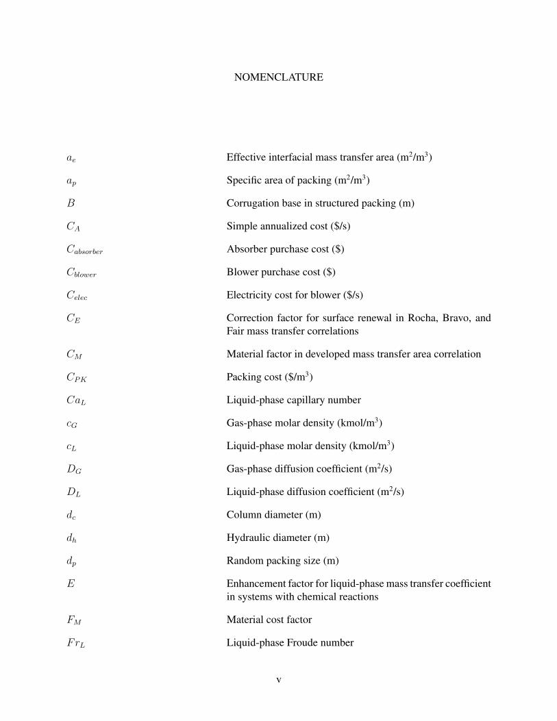
NOMENCLATURE

ae Effective interfacial mass transfer area (m2/m3)

ap Specific area of packing (m2/m3)

B Corrugation base in structured packing (m)

CA Simple annualized cost ($/s)

Cabsorber Absorber purchase cost ($)

Cblower Blower purchase cost ($)

Celec Electricity cost for blower ($/s)

CE Correction factor for surface renewal in Rocha, Bravo, andFair mass transfer correlations

CM Material factor in developed mass transfer area correlation

CPK Packing cost ($/m3)

CaL Liquid-phase capillary number

cG Gas-phase molar density (kmol/m3)

cL Liquid-phase molar density (kmol/m3)

DG Gas-phase diffusion coefficient (m2/s)

DL Liquid-phase diffusion coefficient (m2/s)

dc Column diameter (m)

dh Hydraulic diameter (m)

dp Random packing size (m)

E Enhancement factor for liquid-phase mass transfer coefficientin systems with chemical reactions

FM Material cost factor

FrL Liquid-phase Froude number

v

FSE Surface enhancement factor in Rocha, Bravo, and Fair masstransfer correlations

G Gas-phase molar flow rate (kmol/s)

g Acceleration due to gravity (m/s2)

geff Effective acceleration due to gravity in Rocha, Bravo, andFair mass transfer correlations (m/s2)

HA Henry’s law constant for component A (Pa)

h Corrugation height in structured packing (m)

hL Liquid holdup

KOG Overall gas-phase mass transfer coefficient (m/s)

KOL Overall liquid-phase mass transfer coefficient (m/s)

kG Gas-phase mass transfer coefficient (m/s)

kL Liquid-phase mass transfer coefficient (m/s)

kOH− CO2-NaOH reaction rate constant (m3/kmol s)

L Liquid-phase molar flow rate (kmol/s)

lτ Length of flow path in Billet and Schultes mass transfer cor-relations (m)

NA Mass transfer flux of component A (kmol/s)

P Pressure (Pa)

PB Blower power (W)

Pd Column design pressure (Pa)

Pstress Maximum allowable column stress (Pa)

∆Pd Dry pressure drop (Pa)

R Ideal gas constant (kJ/kmol K)

ReG Gas-phase Reynolds number

ReL Liquid-phase Reynolds number

S Side dimension of corrugation in structured packing (m)

vi

ScG Gas-phase Schmidt number

ScL Liquid-phase Schmidt number

ShG Gas-phase Sherwood number

T Temperature (K)

ts Column shell thickness (m)

uG Gas-phase superficial velocity (m/s)

uGe Gas-phase effective velocity (m/s)

uL Liquid-phase superficial velocity (m/s)

uLe Liquid-phase effective velocity (m/s)

VPK Packing volume (m3)

W Column weight (kg)

WeL Liquid-phase Weber number

xA Liquid-phase mole fraction of component A (mol/mol)

xiA Liquid-phase mole fraction of component A at gas-liquid in-

terface (mol/mol)

x∗A Equilibrium liquid-phase mole fraction of component A

(mol/mol)

xA,in Liquid-phase mole fraction of component A entering column(mol/mol)

xA,out Liquid-phase mole fraction of component A exiting column(mol/mol)

yA Gas-phase mole fraction of component A (mol/mol)

yiA Gas-phase mole fraction of component A at gas-liquidinterface(mol/mol)

y∗A Equilibruim gas-phase mole fraction of component A(mol/mol)

yA,in Gas-phase mole fraction of component A entering column(mol/mol)

vii

yA,out Gas-phase mole fraction of component A exiting column(mol/mol)

Z Height of packing (m)

Greek Letters

α Corrugation angle in structured packing (°)

γ Contact angle in Rocha, Bravo, and Fair mass transfer corre-lations (°)

δNusselt Nusselt film thickness (m)

ε Void fraction of packing

µG Gas-phase dynamic viscosity (Pa s)

µL Liquid-phase dynamic viscosity (Pa s)

ρG Gas-phase density (kg/m3)

ρL Liquid-phase density (kg/m3)

ρM Column shell material of construction density (kg/m3)

σ Surface tension (N/m)

σc Critical surface tension in Onda mass transfer correlations(N/m)

viii

TABLE OF CONTENTS

Page

ABSTRACT . . . . . . . . . . . . . . . . . . . . . . . . . . . . . . . . . . . . . . . . . . . . . . . . . . . . . . . . . . . . . . . . . . . . . . . . . . . . . . . . . . . . . . . . . ii

ACKNOWLEDGMENTS . . . . . . . . . . . . . . . . . . . . . . . . . . . . . . . . . . . . . . . . . . . . . . . . . . . . . . . . . . . . . . . . . . . . . . . . . . iii

CONTRIBUTORS AND FUNDING SOURCES . . . . . . . . . . . . . . . . . . . . . . . . . . . . . . . . . . . . . . . . . . . . . . . . . iv

NOMENCLATURE . . . . . . . . . . . . . . . . . . . . . . . . . . . . . . . . . . . . . . . . . . . . . . . . . . . . . . . . . . . . . . . . . . . . . . . . . . . . . . . . . v

TABLE OF CONTENTS . . . . . . . . . . . . . . . . . . . . . . . . . . . . . . . . . . . . . . . . . . . . . . . . . . . . . . . . . . . . . . . . . . . . . . . . . . . ix

LIST OF FIGURES . . . . . . . . . . . . . . . . . . . . . . . . . . . . . . . . . . . . . . . . . . . . . . . . . . . . . . . . . . . . . . . . . . . . . . . . . . . . . . . . . xi

LIST OF TABLES. . . . . . . . . . . . . . . . . . . . . . . . . . . . . . . . . . . . . . . . . . . . . . . . . . . . . . . . . . . . . . . . . . . . . . . . . . . . . . . . . . . xii

1. INTRODUCTION. . . . . . . . . . . . . . . . . . . . . . . . . . . . . . . . . . . . . . . . . . . . . . . . . . . . . . . . . . . . . . . . . . . . . . . . . . . . . . . 1

1.1 Climate Change and CO2 Absorption. . . . . . . . . . . . . . . . . . . . . . . . . . . . . . . . . . . . . . . . . . . . . . . . . . . . 11.2 Packed Columns . . . . . . . . . . . . . . . . . . . . . . . . . . . . . . . . . . . . . . . . . . . . . . . . . . . . . . . . . . . . . . . . . . . . . . . . . . 4

1.2.1 Random Packing . . . . . . . . . . . . . . . . . . . . . . . . . . . . . . . . . . . . . . . . . . . . . . . . . . . . . . . . . . . . . . . . . 41.2.2 Structured Packing . . . . . . . . . . . . . . . . . . . . . . . . . . . . . . . . . . . . . . . . . . . . . . . . . . . . . . . . . . . . . . . 5

1.3 Mass Transfer Modeling . . . . . . . . . . . . . . . . . . . . . . . . . . . . . . . . . . . . . . . . . . . . . . . . . . . . . . . . . . . . . . . . . . 7

2. LITERATURE REVIEW .. . . . . . . . . . . . . . . . . . . . . . . . . . . . . . . . . . . . . . . . . . . . . . . . . . . . . . . . . . . . . . . . . . . . . . 11

2.1 Mass Transfer Correlations . . . . . . . . . . . . . . . . . . . . . . . . . . . . . . . . . . . . . . . . . . . . . . . . . . . . . . . . . . . . . . . 112.2 Packed Column Data. . . . . . . . . . . . . . . . . . . . . . . . . . . . . . . . . . . . . . . . . . . . . . . . . . . . . . . . . . . . . . . . . . . . . . 17

3. PROBLEM STATEMENT AND APPROACH . . . . . . . . . . . . . . . . . . . . . . . . . . . . . . . . . . . . . . . . . . . . . . . . 21

3.1 Problem Statement . . . . . . . . . . . . . . . . . . . . . . . . . . . . . . . . . . . . . . . . . . . . . . . . . . . . . . . . . . . . . . . . . . . . . . . . 213.2 Approach . . . . . . . . . . . . . . . . . . . . . . . . . . . . . . . . . . . . . . . . . . . . . . . . . . . . . . . . . . . . . . . . . . . . . . . . . . . . . . . . . . 22

4. METHODOLOGY . . . . . . . . . . . . . . . . . . . . . . . . . . . . . . . . . . . . . . . . . . . . . . . . . . . . . . . . . . . . . . . . . . . . . . . . . . . . . . 24

4.1 Mass Transfer Correlation Development . . . . . . . . . . . . . . . . . . . . . . . . . . . . . . . . . . . . . . . . . . . . . . . . 244.2 Mass Transfer Correlation Comparison. . . . . . . . . . . . . . . . . . . . . . . . . . . . . . . . . . . . . . . . . . . . . . . . . . 274.3 ProMax Model Development . . . . . . . . . . . . . . . . . . . . . . . . . . . . . . . . . . . . . . . . . . . . . . . . . . . . . . . . . . . . . 284.4 Design and Economic Analysis . . . . . . . . . . . . . . . . . . . . . . . . . . . . . . . . . . . . . . . . . . . . . . . . . . . . . . . . . . 30

5. RESULTS AND DISCUSSION . . . . . . . . . . . . . . . . . . . . . . . . . . . . . . . . . . . . . . . . . . . . . . . . . . . . . . . . . . . . . . . . 38

ix

5.1 Mass Transfer Correlation Development . . . . . . . . . . . . . . . . . . . . . . . . . . . . . . . . . . . . . . . . . . . . . . . . 385.1.1 Effective Interfacial Mass Transfer Area. . . . . . . . . . . . . . . . . . . . . . . . . . . . . . . . . . . . . . . . 385.1.2 Gas and Liquid Phase Mass Transfer Coefficients . . . . . . . . . . . . . . . . . . . . . . . . . . . . . 44

5.2 Mass Transfer Correlation Comparison. . . . . . . . . . . . . . . . . . . . . . . . . . . . . . . . . . . . . . . . . . . . . . . . . . 465.3 Design and Economic Analysis . . . . . . . . . . . . . . . . . . . . . . . . . . . . . . . . . . . . . . . . . . . . . . . . . . . . . . . . . . 49

6. CONCLUSIONS . . . . . . . . . . . . . . . . . . . . . . . . . . . . . . . . . . . . . . . . . . . . . . . . . . . . . . . . . . . . . . . . . . . . . . . . . . . . . . . 51

REFERENCES . . . . . . . . . . . . . . . . . . . . . . . . . . . . . . . . . . . . . . . . . . . . . . . . . . . . . . . . . . . . . . . . . . . . . . . . . . . . . . . . . . . . . . 52

APPENDIX A. USER DEFINED MASS TRANSFER CORRELATION CODE . . . . . . . . . . . . . . 55

APPENDIX B. ADDITIONS TO PROMAX COLUMNHARDWARE.XML FILE . . . . . . . . . . . 61

x

LIST OF FIGURES

FIGURE Page

1.1 Process flow diagram for a generic CO2 absorption process. . . . . . . . . . . . . . . . . . . . . . . . . . . . 2

1.2 Examples of different types of random packing. (a) Raschig ring. (b) Berl saddle.(c) and (d) Pall ring. (e) Intalox saddle. (f) Super Intalox saddle. Reprinted from[Green and Perry, 2008] . . . . . . . . . . . . . . . . . . . . . . . . . . . . . . . . . . . . . . . . . . . . . . . . . . . . . . . . . . . . . . . . . . 5

1.3 Examples of structured packing. Reprinted from [Kister, 1992] . . . . . . . . . . . . . . . . . . . . . . . 6

1.4 Diagram of structured packing dimensions. Reprinted from [Olujic et al., 2001] . . . . . 6

1.5 Material balance on a differential element of a packed column.. . . . . . . . . . . . . . . . . . . . . . . . 7

3.1 Thesis workflow diagram. . . . . . . . . . . . . . . . . . . . . . . . . . . . . . . . . . . . . . . . . . . . . . . . . . . . . . . . . . . . . . . . . 22

4.1 ProMax absorber flowsheet. . . . . . . . . . . . . . . . . . . . . . . . . . . . . . . . . . . . . . . . . . . . . . . . . . . . . . . . . . . . . . . 32

5.1 Mellapak 250Y effective interfacial mass transfer area vs liquid superficial velocityfor different gas superficial velocities. . . . . . . . . . . . . . . . . . . . . . . . . . . . . . . . . . . . . . . . . . . . . . . . . . . . 38

5.2 GT-OPTIM PAK 250Y effective interfacial mass transfer area vs liquid superficialvelocity for different liquid viscosities. . . . . . . . . . . . . . . . . . . . . . . . . . . . . . . . . . . . . . . . . . . . . . . . . . . 39

5.3 Mellapak 125Y effective interfacial mass transfer area vs liquid superficial velocityfor different surface tensions. . . . . . . . . . . . . . . . . . . . . . . . . . . . . . . . . . . . . . . . . . . . . . . . . . . . . . . . . . . . . 40

5.4 Effective interfacial mass transfer area vs liquid superficial velocity for differentcorrugation angles (GT-PAK 350Y: 45°, GT-PAK 350Z: 70°). . . . . . . . . . . . . . . . . . . . . . . . . . 41

5.5 % error of ae calculated by Equation 5.4 for random packings. . . . . . . . . . . . . . . . . . . . . . . . . 42

5.6 % error of ae calculated by Equation 5.4 for structured packings. . . . . . . . . . . . . . . . . . . . . . 43

5.7 % error of kG calculated by Equation 5.10 for all packings. . . . . . . . . . . . . . . . . . . . . . . . . . . . . 45

5.8 % error of kL calculated by Equation 5.11 for all packings. . . . . . . . . . . . . . . . . . . . . . . . . . . . . 46

5.9 Predictions of Mellapak 250Y effective interfacial mass transfer area from corre-lations for structured packing. . . . . . . . . . . . . . . . . . . . . . . . . . . . . . . . . . . . . . . . . . . . . . . . . . . . . . . . . . . . . 47

5.10 Predictions of Raschig Super-Rings 1.5 effective interfacial mass transfer areafrom correlations for random packing. . . . . . . . . . . . . . . . . . . . . . . . . . . . . . . . . . . . . . . . . . . . . . . . . . . . 48

xi

LIST OF TABLES

TABLE Page

2.1 Systems used in literature mass transfer correlations. . . . . . . . . . . . . . . . . . . . . . . . . . . . . . . . . . . . 11

2.2 Random packings used in literature mass transfer correlations. . . . . . . . . . . . . . . . . . . . . . . . . 12

2.3 Structured packings used in literature mass transfer correlations. . . . . . . . . . . . . . . . . . . . . . . 12

2.4 Critical surface tension values for common packing materials. . . . . . . . . . . . . . . . . . . . . . . . . 13

4.1 Sources of mass transfer data. . . . . . . . . . . . . . . . . . . . . . . . . . . . . . . . . . . . . . . . . . . . . . . . . . . . . . . . . . . . . 24

4.2 Random packing properties and number of available data points. *Values esti-mated based on similar packings. . . . . . . . . . . . . . . . . . . . . . . . . . . . . . . . . . . . . . . . . . . . . . . . . . . . . . . . . 25

4.3 Structured packing properties and number of available data points. *Values esti-mated based on similar packings. . . . . . . . . . . . . . . . . . . . . . . . . . . . . . . . . . . . . . . . . . . . . . . . . . . . . . . . . 25

4.4 Values of packing-specific constants used in Billet and Schultes correlations. . . . . . . . . 28

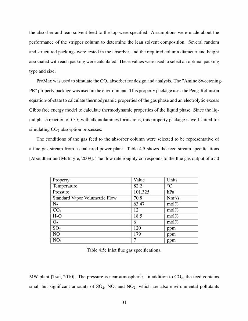
4.5 Inlet flue gas specifications. . . . . . . . . . . . . . . . . . . . . . . . . . . . . . . . . . . . . . . . . . . . . . . . . . . . . . . . . . . . . . . 31

4.6 Components of absorber purchase cost. . . . . . . . . . . . . . . . . . . . . . . . . . . . . . . . . . . . . . . . . . . . . . . . . . 35

5.1 Range of C0 in Equation 5.2 when variable values are systematically adjusted. . . . . . . 44

5.2 % error of ae calculated by correlations. . . . . . . . . . . . . . . . . . . . . . . . . . . . . . . . . . . . . . . . . . . . . . . . . . 48

5.3 % error of kG calculated by correlations. . . . . . . . . . . . . . . . . . . . . . . . . . . . . . . . . . . . . . . . . . . . . . . . . 49

5.4 % error of kL calculated by correlations. . . . . . . . . . . . . . . . . . . . . . . . . . . . . . . . . . . . . . . . . . . . . . . . . 49

5.5 ProMax simulation results for each tested packing. . . . . . . . . . . . . . . . . . . . . . . . . . . . . . . . . . . . . . 50

5.6 CO2 absorption unit costs associated with each tested packing. . . . . . . . . . . . . . . . . . . . . . . . . 50

xii

1. INTRODUCTION

1.1 Climate Change and CO2 Absorption

Concern for anthropogenic climate change has prompted efforts to reduce the environmental

impact of the energy industry. Generation of electrical power is still largely dependent on fossil

fuel use, and fossil fuel use is the most common source of greenhouse gas emissions, mainly in

the form of CO2 released post-combustion [EIA, 2020]. In the United States, combustion of fossil

fuels accounts for approximately 63% of electricity produced [EPA, 2018]. As a result, 27% of all

2018 US greenhouse gas emissions could be attributed to electricity production. Complete phasing

out of fossil fuel combustion in the near future is unlikely given its prevalence, so reduction of

greenhouse gas emissions from existing combustion processes is an important target for climate

change mitigation.

Carbon capture and storage technologies are a family of processes that separate CO2 from

gas mixtures and dispose of it without venting to the atmosphere. When retrofitted to flue gas

streams in power plants, they offer a way to reduce CO2 emissions from fossil fuel combustion.

Several technologies have been developed for this purpose, including absorption, adsorption, cryo-

genic distillation, and membrane processes [Rao and Rubin, 2002]. Among these, absorption is

considered to be the most generally well-suited and feasible for several reasons. First, absorption

processes are effective for feed streams with dilute CO2 concentrations. This is important for car-

bon capture processes because flue gases from coal and natural gas plants are often less than 12%

CO2 by volume. Second, absorption processes are already widely used in industry. They are the

standard technology for many gas treating applications, such as acid gas removal from natural gas,

tail gas treating in sulfur recovery units, and CO2 removal from syngas in ammonia production.

Third, they can be easily scaled. The main unit operations used in absorption are staged columns,

heat exchangers, and pumps, which are all commercially available in a variety of sizes. Finally,

absorption processes can be operated at relatively mild conditions. Temperatures typically range

1

from ambient to 120°C, and pressures typically range from atmospheric to 250 kPa. As a result, ab-

sorption processes incur moderately low equipment costs, utility costs, and safety risks compared

to other carbon capture technologies.

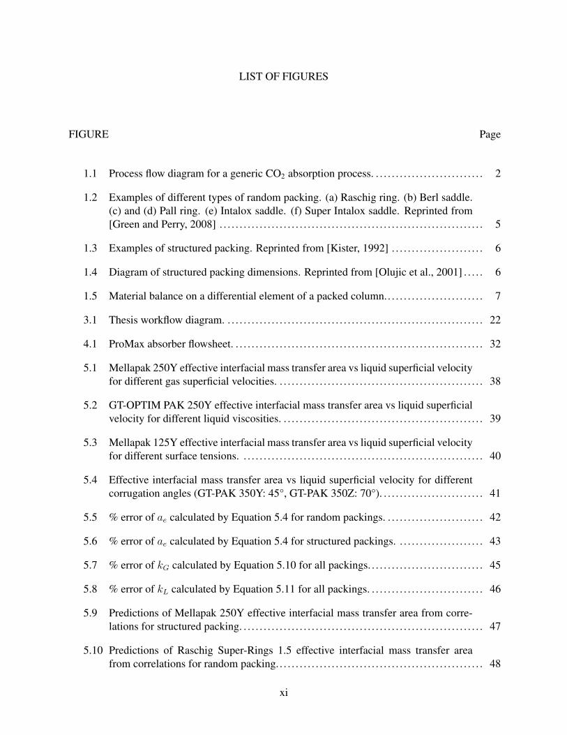
Figure 1.1: Process flow diagram for a generic CO2 absorption process.

A generalized absorption process is shown in Figure 1.1. The flue gas feed stream enters the

bottom of a staged column, typically referred to as the absorber or contactor. Here, the flue gas is

brought into contact with a liquid solvent via countercurrent flow across the column internals. CO2

gets absorbed by the solvent physically or through a chemical reaction, and the treated flue gas

exits the top of the absorber. The rich solvent exits the bottom of the absorber and is sent to the top

of a second staged column called the stripper or regenerator. The absorbed CO2 reenters the vapor

phase as the solvent flows down the column internals and exits the top of the stripper. A partial

condenser helps to further enrich the CO2 product stream and provide reflux. The lean solvent exits

2

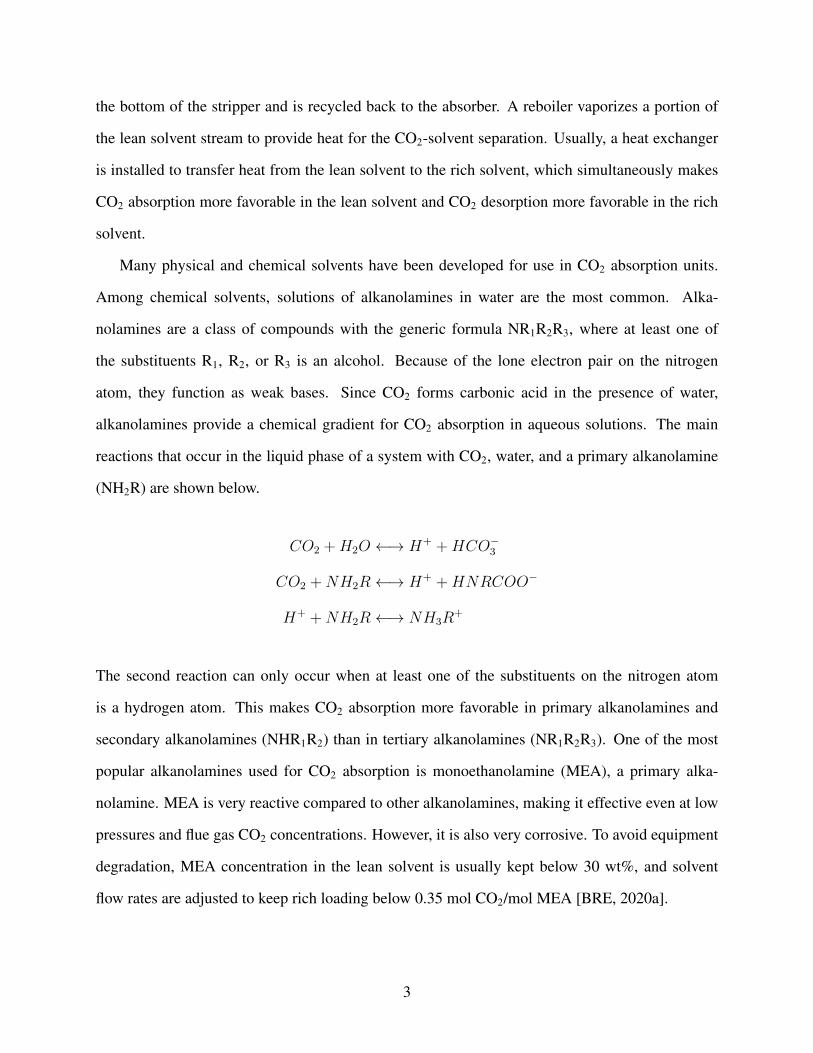
the bottom of the stripper and is recycled back to the absorber. A reboiler vaporizes a portion of

the lean solvent stream to provide heat for the CO2-solvent separation. Usually, a heat exchanger

is installed to transfer heat from the lean solvent to the rich solvent, which simultaneously makes

CO2 absorption more favorable in the lean solvent and CO2 desorption more favorable in the rich

solvent.

Many physical and chemical solvents have been developed for use in CO2 absorption units.

Among chemical solvents, solutions of alkanolamines in water are the most common. Alka-

nolamines are a class of compounds with the generic formula NR1R2R3, where at least one of

the substituents R1, R2, or R3 is an alcohol. Because of the lone electron pair on the nitrogen

atom, they function as weak bases. Since CO2 forms carbonic acid in the presence of water,

alkanolamines provide a chemical gradient for CO2 absorption in aqueous solutions. The main

reactions that occur in the liquid phase of a system with CO2, water, and a primary alkanolamine

(NH2R) are shown below.

CO2 +H2O ←→ H+ +HCO−3

CO2 +NH2R←→ H+ +HNRCOO−

H+ +NH2R←→ NH3R+

The second reaction can only occur when at least one of the substituents on the nitrogen atom

is a hydrogen atom. This makes CO2 absorption more favorable in primary alkanolamines and

secondary alkanolamines (NHR1R2) than in tertiary alkanolamines (NR1R2R3). One of the most

popular alkanolamines used for CO2 absorption is monoethanolamine (MEA), a primary alka-

nolamine. MEA is very reactive compared to other alkanolamines, making it effective even at low

pressures and flue gas CO2 concentrations. However, it is also very corrosive. To avoid equipment

degradation, MEA concentration in the lean solvent is usually kept below 30 wt%, and solvent

flow rates are adjusted to keep rich loading below 0.35 mol CO2/mol MEA [BRE, 2020a].

3

1.2 Packed Columns

Trays or packing may be used as column internals for the absorber and stripper in a CO2 ab-

sorption unit. The choice of which type of internals to use has significant implications for unit

performance, capital cost, and maintenance. Generally, the objective is to maximize the surface

area available for gas-liquid contact inside the column while minimizing pressure drop and issues

associated with installation and upkeep. In terms of these goals, packing can offer several advan-

tages over trays [Towler and Sinnott, 2013]. First, packing typically incurs a lower pressure drop

than trays. This is a significant advantage in CO2 capture applications, where the flue gas feed

often exits the power plant near atmospheric pressure. Second, packing is easier to install and

maintain in columns with a small diameter. Because of this, packed columns can be designed for

a wider range of scales. Third, packing typically offers a lower liquid holdup. Reducing liquid

holdup improves safety and can decreases the rate of equipment degradation in systems with caus-

tic liquids, such as MEA. Finally, packing is associated with a lower tendency for foaming, which

can both reduce gas-liquid contact area and increase pressure drop.

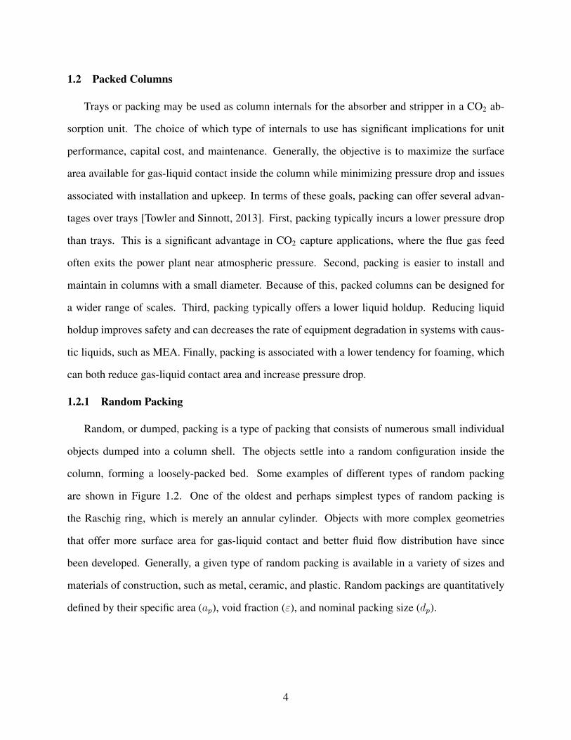
1.2.1 Random Packing

Random, or dumped, packing is a type of packing that consists of numerous small individual

objects dumped into a column shell. The objects settle into a random configuration inside the

column, forming a loosely-packed bed. Some examples of different types of random packing

are shown in Figure 1.2. One of the oldest and perhaps simplest types of random packing is

the Raschig ring, which is merely an annular cylinder. Objects with more complex geometries

that offer more surface area for gas-liquid contact and better fluid flow distribution have since

been developed. Generally, a given type of random packing is available in a variety of sizes and

materials of construction, such as metal, ceramic, and plastic. Random packings are quantitatively

defined by their specific area (ap), void fraction (ε), and nominal packing size (dp).

4

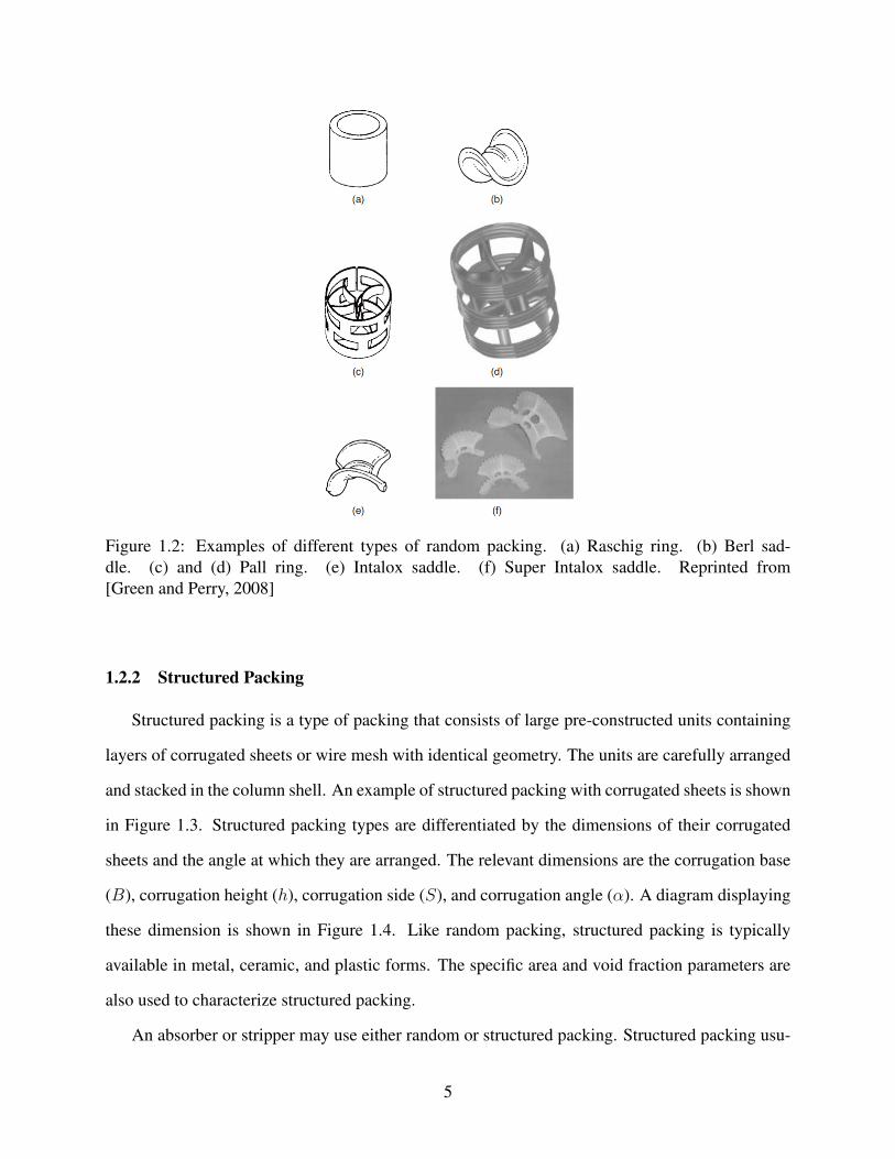
Figure 1.2: Examples of different types of random packing. (a) Raschig ring. (b) Berl sad-dle. (c) and (d) Pall ring. (e) Intalox saddle. (f) Super Intalox saddle. Reprinted from[Green and Perry, 2008]

1.2.2 Structured Packing

Structured packing is a type of packing that consists of large pre-constructed units containing

layers of corrugated sheets or wire mesh with identical geometry. The units are carefully arranged

and stacked in the column shell. An example of structured packing with corrugated sheets is shown

in Figure 1.3. Structured packing types are differentiated by the dimensions of their corrugated

sheets and the angle at which they are arranged. The relevant dimensions are the corrugation base

(B), corrugation height (h), corrugation side (S), and corrugation angle (α). A diagram displaying

these dimension is shown in Figure 1.4. Like random packing, structured packing is typically

available in metal, ceramic, and plastic forms. The specific area and void fraction parameters are

also used to characterize structured packing.

An absorber or stripper may use either random or structured packing. Structured packing usu-

5

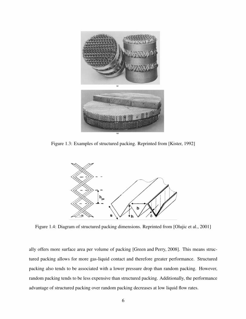
Figure 1.3: Examples of structured packing. Reprinted from [Kister, 1992]

Figure 1.4: Diagram of structured packing dimensions. Reprinted from [Olujic et al., 2001]

ally offers more surface area per volume of packing [Green and Perry, 2008]. This means struc-

tured packing allows for more gas-liquid contact and therefore greater performance. Structured

packing also tends to be associated with a lower pressure drop than random packing. However,

random packing tends to be less expensive than structured packing. Additionally, the performance

advantage of structured packing over random packing decreases at low liquid flow rates.

6

1.3 Mass Transfer Modeling

Rigorous modeling of the absorber and stripper in a CO2 absorption unit is important for proper

design. Overestimation of the performance of either column can result in a unit that is unable to

meet targeted CO2 concentration specifications in the treated flue gas, while underestimation can

result in excess capital costs. In a column with random or structured packing, gas-liquid contact

occurs continuously throughout the height of the packing. This differs from a column with trays, in

which gas-liquid contact is mostly confined to the surface of each tray. A vapor-liquid equilibrium

(VLE) model, which assumes the gas and liquid are in equilibrium a finite number of times in the

column, is therefore more appropriate for a trayed column than a packed column. A mass transfer

model, which considers continuous interchange of components between the gas and liquid phases,

is more appropriate than a VLE model for packed columns [Skowlund et al., 2012].

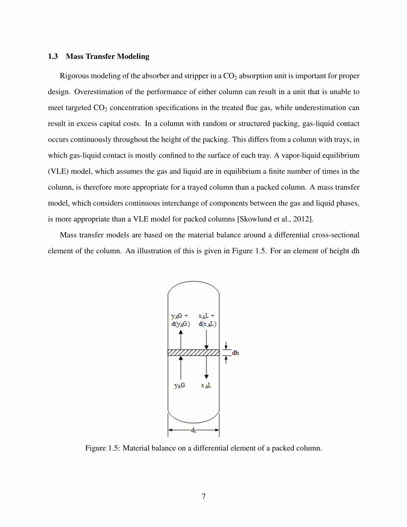
Mass transfer models are based on the material balance around a differential cross-sectional

element of the column. An illustration of this is given in Figure 1.5. For an element of height dh

Figure 1.5: Material balance on a differential element of a packed column.

7

inside the column, the material balance for component A in the gas phase is given in Equation 1.1.

− d(yAG) = NAaeπ

(dc2

)2

dh (1.1)

Here, NA is the mass transfer flux of component A from the gas phase to the liquid phase and ae is

the effective interfacial mass transfer area. NA can be represented in a variety of ways. The most

useful representation for the calculation of concentration profiles in a column is given in Equation

1.2,

NA = KOGcG(yA − y∗A) (1.2)

where KOG is the overall gas phase mass transfer coefficient and y∗A is the equilibrium mole fraction

of component A in the gas phase. KOG can be calculated by considering the other ways NA can

be represented. Due to conservation of mass, the mass transfer flux of component A from the gas

phase to the liquid phase is equal to the mass transfer flux of component A from the bulk gas phase

to the gas-liquid interface (Equation 1.3) and from the gas-liquid interface to the bulk liquid phase

(Equation 1.4).

NA = kGcG(yA − yiA) (1.3)

NA = kLcL(xiA − xA) (1.4)

kG and kL are the gas and liquid phase mass transfer coefficients, respectively, which govern mass

transfer from the bulk phase to the phase interface. yiA and xiA are the gas and liquid phase mole

fractions at the gas-liquid interface, respectively. From these equations for NA, the inverse of the

overall gas phase mass transfer coefficient can be expressed as Equation 1.5.

1

KOG

=1

kG+

1

kL

cGcL

yiA − y∗AxiA − xA

(1.5)

Assuming component A is dilute in the liquid phase, Equation 1.5 can be simplified to Equation

8

1.61

KOG

=1

kG+

1

kL

cGcL

HA

P(1.6)

where HA is the Henry’s law constant for component A.

Equations 1.1, 1.2, and 1.6 are useful for modeling the absorber or stripper in a CO2 absorption

unit when a physical solvent is used. When a chemical solvent, such as MEA, is used, the liquid

phase mass transfer coefficient must be multiplied by an enhancement factor to account for the

chemical reaction that occurs in the liquid phase. Equation 1.6 then becomes

1

KOG

=1

kG+

1

EkL

cGcL

HA

P(1.7)

where E is the enhancement factor. In this case, kL only describes the mass transfer that drives

physical absorption of component A, and E has a value greater than or equal to 1 to account for

the increase in mass transfer rate caused by the reaction. The expression for E depends on the rate

expression for the chemical reaction.

kG, kL, and ae must be known to calculate the mass transfer flux of a component from the

gas phase to the liquid phase. These parameters are usually calculated using correlations from

mechanistic, empirical, or semi-empirical models. When empirical or semi-empirical models are

used, the parameters are typically defined via dimensionless expressions to allow for scaling. ae is

calculated in terms of ae/ap, where ap is the specific area, or surface area per unit volume, of the

packing. kG and kL may be calculated in terms of the Sherwood number, which is a dimensionless

representation of the concentration gradient at the gas-liquid interface. For the gas phase, the

Sherwood number is expressed as Equation 1.8.

ShG =kGdhDG

(1.8)

ShG/L =kG/LdhDG/L

(1.9)

9

ScG/L =µG/L

ρG/LDG/L

(1.10)

The liquid phase Sherwood number (ShL) is expressed similarly, but with kG and DG substi-

tuted for the analogous liquid phase parameters. The hydraulic diameter, dh, is a characteristic

length measurement that often has different definitions across different models. Other dimension-

less parameters commonly found in correlations for ae, kG, and kL include the Reynolds number,

Schmidt number, Froude number, and Weber number. Like the Sherwood number, they can be de-

fined for either the gas phase or the liquid phase with analogous expressions. Equations 1.11-1.14

give the definitions for the liquid phase.

ReL =ρLuLdhµL

(1.11)

ScL =µL

ρLDL

(1.12)

FrL =u2L

gdh(1.13)

WeL =u2LρLdhσ

(1.14)

The Reynolds number (Equation 1.11) represents the ratio of inertial to viscous forces in fluid flow

[Incropera et al., 2007]. The Schmidt number (Equation 1.12) represents the ratio of momentum to

mass diffusivity. The Froude number (Equation 1.13) represents the ratio of inertial to gravitational

forces. Finally, the Weber number (Equation 1.14) represents the ratio of inertial to surface tension

forces. Developers of mass transfer correlations often utilize some combination of these dimen-

sionless numbers to indicate the driving forces governing mass transfer. The relative importance

of each driving force can be expressed by regressing exponents for each number in the correlation.

10

2. LITERATURE REVIEW

2.1 Mass Transfer Correlations

Many correlations for gas and liquid phase mass transfer coefficients and effective interfacial

mass transfer area in packed columns have been developed. These correlations differ in the types

of packings for which they are applicable and the range of operating conditions for which they are

accurate. The help files included in the process simulator ProMax give a good overview of the

applicability and limitations of each correlation included in the software. Tables 2.1-2.3 list the

correlations that will be reviewed in this work along with the systems and packings that were used

to develop them [BRE, 2020b].

Author Gas/Liquid Systems Used to Develop CorrelationOnda et al. (1968) CO2/Water, CO2/CCl4, CO2/Methanol, Air/Water, Benzene-

Toluene-Methanol/Water, Ethanol/WaterBravo and Fair (1982) Cyclohexane/n-Heptane, n-Butane/Isobutene, 1-Propanol/Water,

Ethylbenzene/Styrene, Methanol/Ethanol, Ethanol/Water, n-Heptane/Toluene, Benzene/Dichloroethane, Isooctane/Toluene,NH3-Air/Water, O2-Air/Water

Billet and Schultes (1993) CO2/Water, CO2/Methanol, CO2/Aqueous Salt Solutions, Cl2-Air/Water, Air/Methanol, Air/Benzene, Helium/Water, Freon-12/Water, NH3-N2/Water, NH3-Propane/Water, SO2-Air/Water,Acetone-Air/Water, Ethanol-Air/Water, Chlorobenzene/Ethylben-zene, Toluene/n-Octane, Ethanol/Water, Ethylbenzene/Styrene,Methanol/Ethanol, 1,2-Dichloroethane/Toluene

Rocha, Bravo, and Fair (1996) Air/Water, Cyclohexane/n-Heptane, Ethylbenzene/Styrene,Methanol/Ethanol, Chlorobenzene/Ethylbenzene, i-Butane/n-Butane

Hanley and Chen (2012) Hexane/n-Heptane, 1,2-Propylene Glycol/Ethylene Glycol,Ethylbenzene/Styrene, i-Propane/n-Propane, i-Octane/Toluene,D2O/Water, Chlorobenzene/Ethylbenzene, p-Xylene/o-Xylene,Argon/Oxygen, CO2/Aqueous MEA, CO2/Aqueous AMP

Table 2.1: Systems used in literature mass transfer correlations.

11

Author Random Packings Used to Develop CorrelationOnda et al. (1968) Raschig Rings, Berl Saddles, Spheres, RodsBravo and Fair (1982) Berl Saddles, Raschig Rings, Pall RingsBillet and Schultes (1993) Pall Rings, Ralu Rings, NOR PAC Rings, Hiflow Rings, TOP-Pac

Rings, Raschig Rings, VSP Rings, Envi Pac Rings, Bialecki Rings,Tellerettes, Spheres, Berl Saddles, Intalox Saddles

Rocha, Bravo, and Fair (1996) N/AHanley and Chen (2012) IMTP, Pall Rings, Nutter Rings

Table 2.2: Random packings used in literature mass transfer correlations.

Author Structured Packings Used to Develop CorrelationOnda et al. (1968) N/ABravo and Fair (1982) N/ABillet and Schultes (1993) Ralu Pack YC-250, 250; Impulse Packing 50-100; Montz Packing

B1-200, B1-300, C1-200, C2-200; Euroform PN-110Rocha, Bravo, and Fair (1996) FLEXIPAC 2; GEMPAK 2A, 2AT; Intalox 2T; MaxPak; Mellapak

250Y, 350Y, 500Y; Sulzer BXHanley and Chen (2012) Intalox 2T; FLEXIPAC 500Y; Mellapak 250Y, 750Y; Koch-Glitsch

BX, DX, EX

Table 2.3: Structured packings used in literature mass transfer correlations.

Onda et al. developed one of the first widely used set of correlations for mass transfer in

packed columns [Onda et al., 1968]. The correlations, given in Equations 2.1-2.3, utilize empirical

relationships for both mass transfer coefficients and interfacial area.

ShG = 5.23Re0.7G Sc1/3G (apdp)

−2.0 (2.1)

kL

(ρLµLg

)1/3

= 0.0051

(ρLuL

aeµL

)2/3

Sc−1/2L (apdp)

0.4 (2.2)

aeap

= 1− exp

[−1.45

(σC

σ

)0.75

Re0.1L Fr−0.05L We0.2L

](2.3)

The hydraulic diameter used in calculating ShG, ReG, ReL, FrL, and WeL is defined as dh =

1/ap in this context. σc is the critical surface tension, which is a property of packing material of

12

construction. Values of σc for the materials of construction used in developing the correlations

are given in Table 2.4 [Towler and Sinnott, 2013]. The correlations fit the data used to validate

Packing Material of Construction σc (mN/m)Ceramic 61Metal (steel) 75Plastic (polyethylene) 33Carbon 56

Table 2.4: Critical surface tension values for common packing materials.

them within ±20% for absorption cases and ±30% for distillation cases. However, the correlations

were not validated with data from structured packings and therefore are only applicable to random

packings. Furthermore, the random packings used by Onda et al. were early-developed packings

with simple geometries. The correlations preceded the development of modern random packings

with more complex geometries. Another limitation of the Onda correlations is the upper-limit

of 1 imposed on ae/ap by the form of Equation 2.3. This upper-limit assumes that the effective

interfacial mass transfer area cannot be greater than the total surface area of the packing. Since the

descending liquid phase in a packed column can form droplets and waves that provide additional

gas-liquid contact area, this assumption is not necessarily true.

Bravo and Fair further developed the Onda correlations to produce another widely used set of

mass transfer correlations for random packing [Bravo and Fair, 1982]. They left the correlations

for the gas and liquid phase mass transfer coefficients unaltered, but they developed the following

correlation for the effective interfacial mass transfer area:

aeap

= 0.498

(σ(dyn/cm)0.4

Z(ft)0.5

)(6CaLReG)

0.392 (2.4)

CaL is the liquid phase capillary number, which is the liquid phase Weber number divided by the

liquid phase Reynolds number (CaL = WeL/ReL). This correlation for ae/ap removed the upper-

13

limit of 1 imposed by the Onda correlations. However, the range of packing types used to validate

the correlation was still somewhat narrow and excluded structured packings.

Billet and Schultes developed a set of mass transfer correlations validated with a large number

of gas-liquid systems, random packings, and structured packings [Billet and Schultes, 1993]. The

expressions for the gas and liquid phase mass transfer coefficients are based on a fundamental

model for mass transfer called penetration theory, making them somewhat mechanistic. The Billet

and Schultes correlations are given in Equations 2.5-2.7.

kG = CG1

(ε− hL)1/2

DGa1/2p

l1/2τ

(ρGuG

apµG

)3/4

Sc1/3G (2.5)

kL = CL

(ρLg

µL

)1/6(DL

lτ

)1/2(uL

ap

)1/3

(2.6)

aeap

= 1.5 (aplτ )−0.5Re−0.2

L We0.75L Fr−0.45L (2.7)

CG and CL are dimensionless constants that were regressed for various random and structured

packings. lτ is the length of the flow path in penetration theory. In this context, it is equal to the

hydraulic diameter used in calculating ReL, WeL, and FrL. Billet and Schultes used the following

definition:

lτ = dh = 4ε

ap(2.8)

The correlation for kG also used liquid holdup, hL, which was calculated with Equation 2.9.

hL =

(12

1

g

µL

ρLuLa

2p

)1/3

(2.9)

The Billet and Schultes correlations were particularly useful because they were validated for

both random and structured packings. Furthermore, the introduction of the packing-specific con-

stants CG and CL provided a mechanism to address magnitude inaccuracies in applying the cor-

relations to packings not validated in the study. However, CG and CL must be determined experi-

mentally for each packing used with the correlations. Additionally, many popular modern random

14

and structured packings, such as IMTP and the Sulzer Mellapak series, were not used in the devel-

opment of the form of the correlation equations.

Rocha, Bravo, and Fair developed a separate set of correlations that were also inspired by pene-

tration theory [Rocha et al., 1996]. The liquid phase mass transfer coefficient correlation (Equation

2.11) utilized the mechanistic model, while the correlations for the gas phase mass transfer coeffi-

cient (Equation 2.10) and effective interfacial area (Equation 2.12) utilized empirical relationships.

ShG = 0.054

((uGe + uLe) ρGS

µG

)0.8

Sc0.33G (2.10)

kL = 2

(DLCEuLe

πS

)1/2

(2.11)

aeap

= FSE29.12 (WeLFrL)

0.15 S0.359

Re0.2L ε0.6 (1− 0.93 cos γ) (sinα)0.3(2.12)

CE and FSE are dimensionless constants used to account for imperfect surface renewal by the

liquid phase and surface enhancement features present in the packing, respectively. Rocha, Bravo,

and Fair assumed a value of 0.9 for CE , and FSE is a property of the type of packing used. S is the

side length of the corrugation in corrugated sheet structured packing. The hydraulic diameter dh

used in calculating ReL, FrL, and WeL is taken to be equal to S. α is the corrugation angle, or the

angle at which the corrugated sheets in a bundle of structured packing are arranged. γ is defined

as the contact angle, which is taken to be a function of surface tension:

cos γ =

0.9 σ ≤ 0.055N/m

5.211× 10−16.835σ σ > 0.055N/m

(2.13)

The correlations for the mass transfer coefficients use effective velocities for the gas and liquid

phases (uGe and uLe, respectively) rather than superficial velocities. These are given by the follow-

ing expressions:

uGe =uG

ε (1− hL) sinα(2.14)

15

uLe =uL

εhL sinα(2.15)

Like the Billet and Schultes correlations, the Rocha, Bravo, and Fair correlations assume the mass

transfer coefficients have a dependence on liquid holdup. However, Rocha, Bravo, and Fair used a

different correlation to calculate liquid holdup:

hL =

(4

1

FSES

aeap

)2/3(3µLuL

ρLgeffε sinα

)1/3

(2.16)

geff = gρL − ρG

ρL

(1− ∆P/∆Z

1025

)(2.17)

∆P

∆Z=

∆Pd

∆Z

[1

1− (0.614 + 71.35S)hL

]5(2.18)

∆Pd

∆Z=

0.177ρG

Sε2 (sinα)2u2G +

88.774µG

S2ε sinαuG (2.19)

Equations 2.16-2.19 must be solved for hL and ∆P/∆Z. This can be done via iterative substitution

with an initial guess of ∆P/∆Z = ∆Pd/∆Z.

The Rocha, Bravo, and Fair correlations provided a more rigorous model for mass transfer.

They considered several packing-specific parameters, enabling them to capture differences in the

performance of similar packings. However, no random packings were used in the study. Further-

more, many of the packing-specific parameters, such as FSE , S, and α, apply only to corrugated

sheet structured packing with no analog in other packing types. This makes it impossible to use

the correlations with random packings without assuming values for these parameters.

Hanley and Chen developed mass transfer correlations for use in the Aspen Plus process simu-

lator [Hanley and Chen, 2012]. The correlations use empirical relationships for both mass transfer

coefficients and effective interfacial area. Separate correlations were regressed for different pack-

16

ing types. The correlations are given in Equations 2.20-2.22.

ShG =

0.00104ReGSc

1/3G for Metal Pall Rings

0.00473ReGSc1/3G for Metal IMTP

0.0084ReGSc1/3G

(cosα

cosπ/4

)−7.15

for Metal Structured Packing

(2.20)

ShL =

ReLSc

1/3L for Metal Pall Rings and IMTP

0.33ReLSc1/3L for Metal Structured Packing

(2.21)

aeap

=

0.25Re0.134G Re0.205L We0.075L Fr−0.164

L

(ρGρL

)−0.154 (µG

µL

)0.195

for Metal Pall Rings

0.332Re0.132G Re−0.102L We0.194L Fr−0.2

L

(ρGρL

)−0.154 (µG

µL

)0.195

for Metal IMTP

0.539Re0.145G Re−0.153L We0.2L Fr−0.2

L

(ρGρL

)−0.033 (µG

µL

)0.090 (cosα

cosπ/4

)4.078

for Metal Structured Packing(2.22)

The hydraulic diameter in this context is defined as dh = 4ε/ap. Systems with amine solvents

were analyzed in their study, making the Hanley and Chen correlations particularly relevant for

CO2 absorption processes. However, the correlations are purely empirical, and their predictive

ability for packings, systems, and operating conditions outside of those used in the study is ques-

tionable. Even for the packings used in the study, the correlations tend to overestimate the effective

interfacial mass transfer area at low liquid superficial velocities.

2.2 Packed Column Data

The Process Science and Technology Center (PSTC) at the University of Texas in Austin op-

erates a staged column that is used to collect absorption data for both random and structured pack-

ings. Many of these data have been published in theses and dissertations written by graduate

students in the group [Wilson, 2004, Tsai, 2010, Wang, 2015, Song, 2017]. With these theses and

dissertations, the PSTC offers an extensive database for validation of mass transfer correlations.

PSTC mass transfer data comes from experiments with CO2-air/NaOH-water, SO2-air/NaOH-

17

water, and air/toluene-water systems in packed columns. CO2-air/NaOH-water experiments are

used to determine ae, SO2-air/NaOH-water experiments are used to determine kG, and air/toluene-

water experiments are used to determine kL. In CO2-air/NaOH-water experiments, inlet and outlet

gas phase CO2 concentrations and temperatures and the superficial velocities of the gas and liq-

uid phases are measured. With knowledge of these parameters, ae can be calculated by taking

a material balance around the packed column. Assuming CO2 is dilute in the gas phase and the

equilibrium concentration of CO2 in the gas phase is zero, Equations 1.1-1.2 can be simplified and

combined to form Equation 2.23.

− uGdyCO2 = KOGaeyCO2dh (2.23)

Assuming uG, KOG, and ae are constant throughout the column, Equation 2.23 can be integrated

across the height of the column to produce Equation 2.24.

KOGae =uG

Zln

yCO2,in

yCO2,out

(2.24)

Like alkanolamines, NaOH promotes CO2 absorption by facilitating acid-base reactions in the

liquid phase. The liquid phase mass transfer coefficient is therefore amplified by an enhancement

factor, so Equation 1.7 is applicable for this system. If the CO2-NaOH reaction is taken to be first

order, the enhancement factor has the following definition

E =

√1 +

kOH− [OH−]DCO2,L

k2L

(2.25)

where kOH− is the reaction rate constant. The CO2-NaOH reaction is considered to be the rate-

limiting step in CO2 absorption for this system [Wang et al., 2016]. Additionally, the reaction rate

is considered to be much greater than the mass transfer rate of CO2 from the gas-liquid interface

to the bulk liquid phase. Under these circumstances, the 1 term under the square root in Equation

2.25 and the 1/kG term in Equation 1.7 can be negated. Assuming the ideal gas law is valid, this

18

allows for the following approximation

1

KOG

≈ 1√kOH− [OH−]DCO2,L

HCO2

RT(2.26)

Combining Equations 2.24 and 2.26 creates the following expression

ae =uG

ZRT

HCO2√kOH− [OH−]DCO2,L

lnyCO2,in

yCO2,out

(2.27)

which can be used to calculate ae in CO2-air/NaOH-water systems.

The gas phase mass transfer coefficient in a packed column can be calculated with data from

SO2-air/NaOH-water experiments. Like CO2 absorption, SO2 absorption is enhanced by liquid

phase reactions with NaOH. However, NaOH reacts more aggressively with SO2 than CO2. Be-

cause of this, SO2 absorption is considered to be limited by gas phase mass transfer rather than

the reaction with NaOH. This allows for an alternative approximation of Equation 1.7 in which the

liquid phase mass transfer term rather than the gas phase mass transfer term can be negated. For

SO2-air/NaOH-water systems, the following approximation is used

1

KOG

≈ 1

kG(2.28)

which allows for the following analogous form of Equation 2.24.

kG =uG

aeZln

ySO2,in

ySO2,out

(2.29)

Equation 2.29 is used to calculate kG in these experiments. uG, ySO2,in, and ySO2,out are directly

measured. The value of ae is taken from a CO2-air/NaOH-water experiment in which the same

packing and superficial gas and liquid phase velocities were used.

Data from air/toluene-water experiments are used to calculate the liquid phase mass transfer

coefficient. In the air/toluene-water system, toluene is stripped from an aqueous solution by air.

19

Since the component moving between phases originates in the liquid phase, mass transfer is ana-

lyzed from the liquid phase perspective rather than the gas phase perspective. The analogous form

of Equation 1.2 for the liquid phase perspective is

(−NA) = KOLcL(xA − x∗A) (2.30)

where KOL is the overall liquid phase mass transfer coefficient. An analogous form of Equation 1.5

can be used to calculate KOL. Unlike the CO2-air/NaOH-water and SO2-air/NaOH-water systems,

the air/toluene-water system involves no chemical reactions. Toluene stripping is assumed to be

limited by liquid phase mass transfer, so KOL can be approximated as

1

KOL

≈ 1

kL(2.31)

Using this approximation with a mass balance on liquid phase toluene integrated across the height

of the packed column gives Equation 2.32

kL =uL

aeZln

xtoluene,in

xtoluene,out

(2.32)

which can be used to calculate kL. Similar to the SO2-air/NaOH-water experiments, uL, xtoluene,in,

and xtoluene,out are directly measured, while ae is determined from a comparable CO2-air/NaOH-

water experiment.

20

3. PROBLEM STATEMENT AND APPROACH

3.1 Problem Statement

Carbon capture and storage technologies offer a way to reduce greenhouse gas emissions as-

sociated with the US energy industry. Because they can be retrofitted to existing fossil fuel com-

bustion processes, they are a more immediately viable solution than replacement with alternative

energy sources. The most feasible process for carbon capture in the present day is CO2 absorption

with MEA in a staged column, and the use of packing instead of trays inside the column can offer

several advantages. However, rigorous simulation of a packed absorber column for design and

analysis purposes requires mass transfer modeling. This in turn requires knowledge of the gas and

liquid phase mass transfer coefficients and effective interfacial mass transfer area.

Despite the existence of many correlations for mass transfer parameters in literature, no sin-

gle set of correlation is accurate across the entire range of gas/liquid systems, column operating

conditions, and packing types. Furthermore, the continuous development of new types of random

and structured packings inevitably creates scenarios for which a particular mass transfer correla-

tion is not applicable. For these reasons, additional development and validation of mass transfer

correlations with experimental data for random and structured packings is needed.

The objective of this thesis is to develop a set mass transfer correlations and use them in mod-

eling a carbon capture CO2 absorption unit. Correlations will be developed for the gas and liquid

phase mass transfer coefficients and the effective interfacial mass transfer area. The correlations

will consider both extensive and intensive properties of the gas and liquid in the column, such as

superficial velocities, densities, viscosities, and surface tension. They will also consider parameters

specific to the type of packing used and have relevance for both random and structured packings.

Data sets published by the Process Science and Technology Center at the University of Texas in

Austin will be used to validate the correlations and compare their accuracy to that of other literature

correlations. Using the newly developed correlations in conjunction with the process simulation

21

software ProMax, a design and economic analysis of a CO2 absorber column will be performed.

3.2 Approach

A diagram of the workflow for this thesis is given in Figure 3.1. The work of this thesis can be

divided into four main sequential parts.

Figure 3.1: Thesis workflow diagram.

First, published mass transfer data from the PSTC will be used to develop mass transfer cor-

relations for the gas phase mass transfer coefficient, liquid phase mass transfer coefficient, and

22

effective interfacial mass transfer area. This involves consolidating data from several published

theses and dissertations from the PSTC group. The data will be analyzed to observe trends with

respect to gas and liquid phase physical properties, superficial velocities, and packing parameters.

Expressions for the three mass transfer parameters will then be regressed to fit these trends.

Second, predictions from the developed correlations will be compared against those of several

literature correlations and experimentally determined values in the PSTC database. Differences

between the predicted and experimental values of the three mass transfer parameters will be used

to assess the relative accuracy of each correlation.

Third, the developed correlations will be incorporated into ProMax. The correlations will be

made available as a "User Defined" mass transfer correlation in the software’s distillation column

block.

Finally, an absorber for a carbon capture CO2 absorption unit will be designed using the de-

veloped correlations, and an economic analysis of the column will be performed. A model for

an absorber with a feed stream representative of flue gas from a power plant will be simulated in

ProMax. The column height and diameter required to meet a CO2 specification in the treated flue

gas will be determined for several random and structured packings. The capital and utility costs

incurred by each packing will be estimated, and the packing that offers the lowest cost will be

identified as the optimal packing for use in the absorber.

23

4. METHODOLOGY

4.1 Mass Transfer Correlation Development

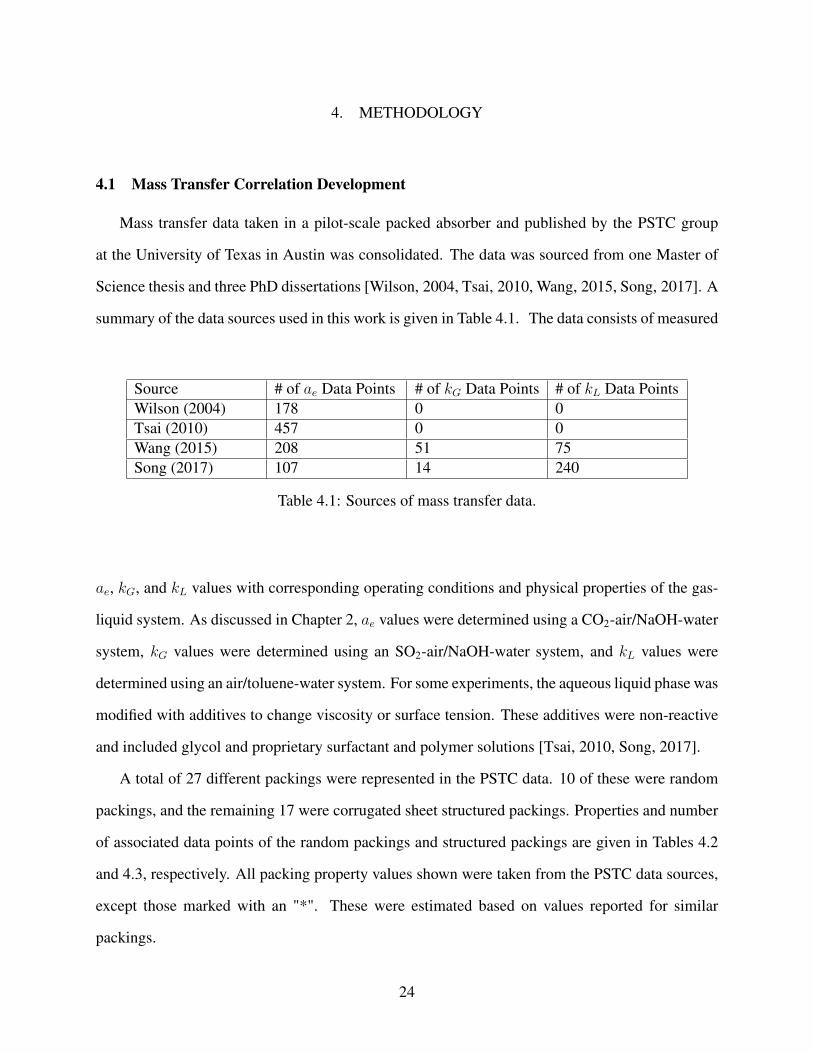
Mass transfer data taken in a pilot-scale packed absorber and published by the PSTC group

at the University of Texas in Austin was consolidated. The data was sourced from one Master of

Science thesis and three PhD dissertations [Wilson, 2004, Tsai, 2010, Wang, 2015, Song, 2017]. A

summary of the data sources used in this work is given in Table 4.1. The data consists of measured

Source # of ae Data Points # of kG Data Points # of kL Data PointsWilson (2004) 178 0 0Tsai (2010) 457 0 0Wang (2015) 208 51 75Song (2017) 107 14 240

Table 4.1: Sources of mass transfer data.

ae, kG, and kL values with corresponding operating conditions and physical properties of the gas-

liquid system. As discussed in Chapter 2, ae values were determined using a CO2-air/NaOH-water

system, kG values were determined using an SO2-air/NaOH-water system, and kL values were

determined using an air/toluene-water system. For some experiments, the aqueous liquid phase was

modified with additives to change viscosity or surface tension. These additives were non-reactive

and included glycol and proprietary surfactant and polymer solutions [Tsai, 2010, Song, 2017].

A total of 27 different packings were represented in the PSTC data. 10 of these were random

packings, and the remaining 17 were corrugated sheet structured packings. Properties and number

of associated data points of the random packings and structured packings are given in Tables 4.2

and 4.3, respectively. All packing property values shown were taken from the PSTC data sources,

except those marked with an "*". These were estimated based on values reported for similar

packings.

24

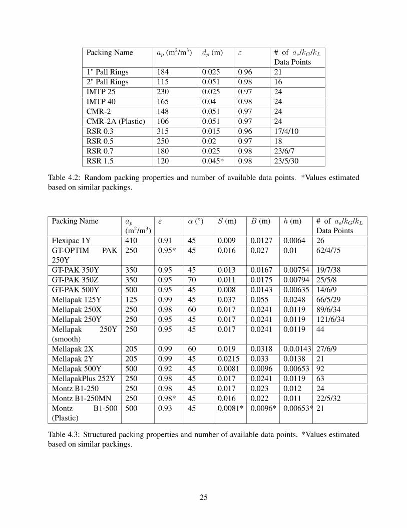
Packing Name ap (m2/m3) dp (m) ε # of ae/kG/kLData Points

1" Pall Rings 184 0.025 0.96 212" Pall Rings 115 0.051 0.98 16IMTP 25 230 0.025 0.97 24IMTP 40 165 0.04 0.98 24CMR-2 148 0.051 0.97 24CMR-2A (Plastic) 106 0.051 0.97 24RSR 0.3 315 0.015 0.96 17/4/10RSR 0.5 250 0.02 0.97 18RSR 0.7 180 0.025 0.98 23/6/7RSR 1.5 120 0.045* 0.98 23/5/30

Table 4.2: Random packing properties and number of available data points. *Values estimatedbased on similar packings.

Packing Name ap(m2/m3)

ε α (°) S (m) B (m) h (m) # of ae/kG/kLData Points

Flexipac 1Y 410 0.91 45 0.009 0.0127 0.0064 26GT-OPTIM PAK250Y

250 0.95* 45 0.016 0.027 0.01 62/4/75

GT-PAK 350Y 350 0.95 45 0.013 0.0167 0.00754 19/7/38GT-PAK 350Z 350 0.95 70 0.011 0.0175 0.00794 25/5/8GT-PAK 500Y 500 0.95 45 0.008 0.0143 0.00635 14/6/9Mellapak 125Y 125 0.99 45 0.037 0.055 0.0248 66/5/29Mellapak 250X 250 0.98 60 0.017 0.0241 0.0119 89/6/34Mellapak 250Y 250 0.95 45 0.017 0.0241 0.0119 121/6/34Mellapak 250Y(smooth)

250 0.95 45 0.017 0.0241 0.0119 44

Mellapak 2X 205 0.99 60 0.019 0.0318 0.0.0143 27/6/9Mellapak 2Y 205 0.99 45 0.0215 0.033 0.0138 21Mellapak 500Y 500 0.92 45 0.0081 0.0096 0.00653 92MellapakPlus 252Y 250 0.98 45 0.017 0.0241 0.0119 63Montz B1-250 250 0.98 45 0.017 0.023 0.012 24Montz B1-250MN 250 0.98* 45 0.016 0.022 0.011 22/5/32Montz B1-500(Plastic)

500 0.93 45 0.0081* 0.0096* 0.00653* 21

Table 4.3: Structured packing properties and number of available data points. *Values estimatedbased on similar packings.

25

Overall, the packing specific areas ranged from 106 to 500m2/m3. The random packings were

modern random packings with complex geometries. Four different types were included: Pall rings,

Intalox Metal Tower Packing (IMTP), Cascade Mini-Rings (CMR), and Raschig Super-Rings

(RSR). For each type, multiple sizes were tested. Similarly, the structured packings consisted of

sets from four types: Flexipac, GT-PAK (including GT-OPTIM PAK), Mellapak (including Mel-

lapakPlus), and Montz. Various corrugation angles and corrugation dimensions were represented.

One plastic random packing and one plastic structured packing (CMR-2A and Montz B1-500,

respectively) were used, with the remaining packings being metal.

The physical properties varied in the PSTC ae experiments were uL, uG, µL, ρL, and σ. ρL was

not varied directly; differences in ρL throughout the database were attributable to minute changes

in column temperature and introduction of non-reactive liquid additives meant to change σ or

µL. Therefore, trends in ae with respect to uL, uG, µL, and σ were analyzed as a starting point for

developing a correlation to fit the data. The properties that were believed to have a significant effect

on ae were organized into dimensionless groups, and an expression for the dimensionless effective

interfacial mass transfer area, ae/ap, in terms of these groups was regressed. The expression was

assumed to be of the power law form, where ae/ap is the product of the dimensionless groups and

a constant with each group raised to a certain power. Most literature correlations developed for

effective interfacial mass transfer area, including the ones analyzed in this work, are power law

relationships in terms of dimensionless groups [Hanley and Chen, 2012].

Regression of a correlation for ae consisted of determining values for the exponents of the

dimensionless groups and the constant in the power law relationship. To simplify the regression,

the natural logarithm of both sides of the equation were taken. This made the equation linear with

respect to the power law exponents and the natural logarithm of the constant. The Solver add-in

in Microsoft Excel was used to determine the exponent and constant values that minimized the

sum of the squared ln ae/ap residuals. Since the sum of the squared residuals as a function of the

exponents and natural logarithm of the constant was smooth and quadratic, "GRG Nonlinear" was

used as the algorithm in the solver.

26

The methodology for developing correlations for kG and kL was similar to that of ae. In the

PSTC kG experiments, uL and uG were varied. In the kL experiments, uL, uG, and µL were varied.

Changing values of ρL and DL are also found in the database, but as was the case with ρL in the

ae experiments, these variations were a by-product of variations in µL rather than experimental

design.

4.2 Mass Transfer Correlation Comparison

Predictions from five sets of literature mass transfer correlations were compared against exper-

imental values from the PSTC data and predictions from the mass transfer correlations developed

in this work. The Onda; Bravo and Fair; Billet and Schultes; Rocha, Bravo, and Fair; and Hanley

and Chen correlations were used. Each of these literature correlations is described in Chapter 2.

To avoid correlation misuse, each correlation was only tested with data for packings to which the

correlation is considered applicable. The Onda and Bravo and Fair correlations were tested with

all random packing data points. The Rocha, Bravo, and Fair correlations were tested with all struc-

tured packing data points. The Hanley and Chen correlations were tested with data points for Pall

rings, IMTP, and metal structured packing. Only the Billet and Schultes correlations were tested

with all data points in the PSTC database.

Some of the literature correlations utilize material or packing-specific constants. The Onda

correlation for ae requires a critical surface tension (σc) that depends on packing material of con-

struction. Values in Table 2.4 for metal and plastic were used in evaluating the Onda correlation for

random packings. The Rocha, Bravo, and Fair correlations use a surface enhancement factor (FSE)

to account for the effect of structured packing surface texture on mass transfer. All metal struc-

tured packings analyzed in this work are assumed to have an FSE of 0.35, and all plastic structured

packings are assumed to have an FSE of 0.46. These values are based on reported FSE values for

metal Flexipac and plastic Mellapak packings [Rocha et al., 1993]. Finally, the Billet and Schultes

correlations for mass transfer coefficients utilize dimensionless packing-specific constants (CG and

CL). Relevant values for these constants are given in Table 4.4. Values marked with "*" were taken

from defaults found in ProMax, those marked with "**" are estimated based on values for similar

27

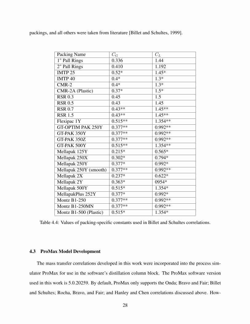
packings, and all others were taken from literature [Billet and Schultes, 1999].

Packing Name CG CL

1" Pall Rings 0.336 1.442" Pall Rings 0.410 1.192IMTP 25 0.52* 1.45*IMTP 40 0.4* 1.3*CMR-2 0.4* 1.3*CMR-2A (Plastic) 0.37* 1.5*RSR 0.3 0.45 1.5RSR 0.5 0.43 1.45RSR 0.7 0.43** 1.45**RSR 1.5 0.43** 1.45**Flexipac 1Y 0.515** 1.354**GT-OPTIM PAK 250Y 0.377** 0.992**GT-PAK 350Y 0.377** 0.992**GT-PAK 350Z 0.377** 0.992**GT-PAK 500Y 0.515** 1.354**Mellapak 125Y 0.215* 0.565*Mellapak 250X 0.302* 0.794*Mellapak 250Y 0.377* 0.992*Mellapak 250Y (smooth) 0.377** 0.992**Mellapak 2X 0.237* 0.622*Mellapak 2Y 0.363* 0954*Mellapak 500Y 0.515* 1.354*MellapakPlus 252Y 0.377* 0.992*Montz B1-250 0.377** 0.992**Montz B1-250MN 0.377** 0.992**Montz B1-500 (Plastic) 0.515* 1.354*

Table 4.4: Values of packing-specific constants used in Billet and Schultes correlations.

4.3 ProMax Model Development

The mass transfer correlations developed in this work were incorporated into the process sim-

ulator ProMax for use in the software’s distillation column block. The ProMax software version

used in this work is 5.0.20259. By default, ProMax only supports the Onda; Bravo and Fair; Billet

and Schultes; Rocha, Bravo, and Fair; and Hanley and Chen correlations discussed above. How-

28

ever, it offers the ability for users to import their own custom set of mass transfer correlations.

Users can then specify for any stage or stages in a distillation column blog to use the custom

correlations instead of one of the aforementioned default correlations to calculate mass transfer

coefficients and effective interfacial area.

A detailed description of how to create and use custom mass transfer correlations is found in

the help files included with the ProMax software [BRE, 2020b]. The help page titled "User Defined

Mass Transfer Coefficient Information" and the "Mass Transfer" section of the "About Advanced

Examples" are particularly relevant. Generally, the process involves writing code to implement

the desired custom correlations, compiling the code into a *.dll assembly, specifying the location

of the assembly in a ProMax distillation column block, and selecting the "User Defined" option

for either "Random Mass Transfer Correlation" or "Structured Mass Transfer Correlation". An

example code project containing implementations of a custom set of correlations (in this case the

Onda correlations) is available in the ProMax example files. The code project can be found by

opening ProMax, selecting "Open Example (as read-only)" in the "Create a new project using"

section of the "ProMax Project Selection" dialog, and navigating to ..\Advanced Examples\Mass

Transfer\UserDefinedMassTransferCoefficients. This code project was used as a starting point for

importing the mass transfer correlations developed in this work into ProMax.

Microsoft Visual Studio was used to open the "UserDefinedMassTransferCoefficients.sln" so-

lution file in the above file path and subsequently view, edit, and compile the example code project.

The Visual Studio solution contains two projects: "CPPCOM_RandomPacking_UDMTC" and

"CSCLR_RandomPacking_UDMTC". Each project contains an implementation of the Onda mass

transfer correlations able to be imported into ProMax. "CPPCOM_RandomPacking_UDMTC" is

written in C++, and "CSCLR_RandomPacking_UDMTC" is written in C#. Only the project writ-

ten in C# was utilized as a basis for implementing the developed mass transfer correlations. Either

project could have been utilized, but the project written in C# was chosen because of the simpler

syntax, smaller amount of required boilerplate code, and author’s familiarity with C# compared to

C++.

29

The "CSCLR_RandomPacking_UDMTC" project contains only one file of relevant C# code,

which is named "CSCLR_UserDefinedMTC.cs". The file contains a class of the same name that

inherits from two ProMax interfaces: "Extensibility.UserDefinedMassTransfer" and "Extensibil-

ity.PersistStreamInit". Methods on these interfaces are called by the ProMax source code to per-

form tasks related to calculating mass transfer parameters and managing resources used in the

calculations. Only three of these methods were actually implemented in the original example code

and later modified to accommodate the code for the developed mass transfer correlation. "InitNew"

is used to create the ProMax properties displayed in the "User Defined Coefficients" tab of the dis-

tillation column block window. "InitBeforeCalculate" is called before ProMax solves a column

block and is used to cache values of properties that do not change throughout the column profile.

Finally, "Individual_K" is called whenever ProMax solves a stage in the column and is used to

calculate the gas and liquid phase mass transfer coefficients and effective interfacial mass transfer

area. Once calculated, the values for the gas and liquid phase coefficients and interfacial area are

assigned to the method’s "KV", "KL", and "Area" arguments, respectively. Since the distillation

column block can handle multicomponent distillation, "KV" and "KL" consist of 2-D N x N arrays

containing binary component mass transfer coefficients, where N is the number of components in

the ProMax environment.

The "InitNew", "InitBeforeCalculated", and "Individual_K" methods in the "CSCLR_ UserDe-

finedMTC" class were modified to replace the Onda mass transfer correlations with the mass trans-

fer correlations developed in this work. The resulting code is given in Appendix A. The solution

containing the code was compiled using the "Release" configuration in Visual Studio, and the pro-

duced *.dll assembly was used as the source of the "User Defined" mass transfer correlation in the

ProMax distillation column block. Details about how the "User Defined" mass transfer correlation

was setup and utilized to simulate a packed CO2 absorber are given in the next section.

4.4 Design and Economic Analysis

A CO2 absorber suitable for post-combustion CO2 capture was designed and analyzed. The

absorber column was simulated in isolation. Conditions for the flue gas feed to the bottom of

30

the absorber and lean solvent feed to the top were specified. Assumptions were made about the

performance of the stripper column to determine the lean solvent composition. Several random

and structured packings were tested in the absorber, and the required column diameter and height

associated with each packing were calculated. These values were used to select an optimal packing

type and size.

ProMax was used to simulate the CO2 absorber for design and analysis. The "Amine Sweetening-

PR" property package was used in the environment. This property package uses the Peng-Robinson

equation-of-state to calculate thermodynamic properties of the gas phase and an electrolytic excess

Gibbs free energy model to calculate thermodynamic properties of the liquid phase. Since the liq-

uid phase reaction of CO2 with alkanolamines forms ions, this property package is well-suited for

simulating CO2 absorption processes.

The conditions of the gas feed to the absorber column were selected to be representative of

a flue gas stream from a coal-fired power plant. Table 4.5 shows the feed stream specifications

[Aboudheir and McIntyre, 2009]. The flow rate roughly corresponds to the flue gas output of a 50

Property Value UnitsTemperature 82.2 °CPressure 101.325 kPaStandard Vapor Volumetric Flow 70.8 Nm3/sN2 63.47 mol%CO2 12 mol%H2O 18.5 mol%O2 6 mol%SO2 120 ppmNO 179 ppmNO2 7 ppm

Table 4.5: Inlet flue gas specifications.

MW plant [Tsai, 2010]. The pressure is near atmospheric. In addition to CO2, the feed contains

small but significant amounts of SO2, NO, and NO2, which are also environmental pollutants

31

readily absorbed by alkanolamine solutions. In some absorption units, a separate absorber column

or column section is used upstream of the absorber for the selective removal of these gases. SO2

in particular is often targeted for removal because it can react with alkanolamines to form heat-

stable salts [BRE, 2020a]. Consistent formation of heat-stable salts reduces the concentration of

alkanolamine in the liquid solvent available for CO2 absorption over time, necessitating additional

process measures to regenerate the solvent. Although avoidance of heat-stable salts is important

to the performance of a CO2 absorption unit, the design and analysis of an SO2 removal system is

omitted from this work for the sake of simplicity.

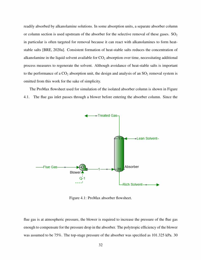
The ProMax flowsheet used for simulation of the isolated absorber column is shown in Figure

4.1. The flue gas inlet passes through a blower before entering the absorber column. Since the

Figure 4.1: ProMax absorber flowsheet.

flue gas is at atmospheric pressure, the blower is required to increase the pressure of the flue gas

enough to compensate for the pressure drop in the absorber. The polytropic efficiency of the blower

was assumed to be 75%. The top-stage pressure of the absorber was specified as 101.325 kPa. 30

32

wt% MEA in water was used as the solvent in the absorption unit. A lean loading of 0.10 mol

CO2/mol MEA, or about 2.17 wt% CO2 in the lean solvent stream, was assumed in the absence of

a simulated regenerator. The flow rate of the solvent was adjusted to make the rich loading 0.35

mol CO2/mol MEA. This was done automatically using a ProMax simple solver set on the standard

liquid volumetric flow rate of the lean solvent. Rich loading was calculated using an amine analysis

on the rich solvent stream and imported into the simple solver as a measured variable. The values

selected for MEA concentration and rich loading correspond to the upper-limit values generally

imposed to limit solvent corrosivity, as discussed in Chapter 1.

The absorber column was modeled using the "Mass + Heat Transfer (Reactive & Non-Reactive)"

model type. "TSWEET Absorber/Stripper" was used for the "Mass + Heat Transfer Column Type"

to account for the kinetics of the liquid phase reactions in the column. The "Mass Transfer For-

mulation" was set to "General Maxwell-Stefan". In the "Stages" tab of the column Project Viewer

window, the "Pressures from Hardware" option was selected. This allowed for the pressure profile

in the column to be calculated rather than user specified. In the "Convergence" tab of the column

Project Viewer window, the "Enthalpy Model" was set to "Composition-Dependent". Selecting this

option seemed to improve the likelihood of column convergence. In the "Mass Transfer" tab, both

the "Random Mass Transfer Correlation" and the "Structured Mass Transfer Correlation" were set

to "User Defined" for all stages. In the "User Defined Coefficients" tab, the "Extensibility Pack-

age Type" was changed to "CLR", and the file path to the compiled *.dll assembly discussed in

Section 4.3 was specified in the "CLR Assembly Name or Path" box. The "CLR Implementation

Class" was specified as "CSCLR_RandomPacking_UDMTC.CSCLR_UserDefinedMTC", which

corresponds to the namespace and class containing the custom mass transfer correlation code. With

these specifications in place, the distillation column block simulating the absorber was set up to use

the mass transfer correlations developed in this work instead of the default correlations in ProMax.

Three random and four structured packings were selected for testing in the isolated absorber

column flowsheet. The random packings were Raschig Super-Rings of size 0.3, 0.7, and 1.5. The

structured packings were Mellapak 125Y, Mellapak 250X, Mellapak 250Y, and GT-PAK 500Y.

33

These seven packings were chosen because they collectively covered much of the range of the

PSTC database in terms of packing properties. The specific areas range from 120 to 500 m2/m3,

void fractions range from 0.95 to 0.99, and structured packing corrugation angles include both

45°and 60°. Additionally, the data for these packings included values for all three mass transfer

parameters (ae, kG, and kL). Using all three of the developed mass transfer correlations in the

context of simulating a CO2 absorber column is therefore less of an extrapolation when considering

these packings than it would be when considering packings for which there was no data available

to fit one of the correlations.

Four of the above seven packings were already available as column hardware options in the

ProMax distillation column block. Raschig Super-Rings of sizes 0.7 and 1.5 and GT-PAK 500Y

had to be implemented as user-defined packings to be used in ProMax. This was done by modi-

fying the "Column Hardware.xml" file. Instructions for doing this were found in the ProMax help

files on the page titled "Column Hardware.xml File" [BRE, 2020b]. Entries for the two random

packings and structured packing were added to the *.xml file. The added *.xml code is shown

in Appendix B. For the new packings added, values of several constants used in the Billet and

Schultes mass transfer and pressure drop correlations were required. The values associated with

the new Raschig Super-Ring sizes were linearly interpolated based on those associated with the

sizes of metal Raschig Super-Rings already available in ProMax (0.3, 0.5, 1, 2, and 3). The values

associated with GT-PAK 500Y were assumed to be the same as those associated with Mellapak

500Y.

Each of the seven packings mentioned above was used in turn to populate all of the absorber

column stage internals, the flowsheet was solved, and a suitable column diameter and height were

determined. For every packing test, 20 column stages were used. The number of stages in a packed

mass and heat transfer model column represents only the number of discrete cross-sectional ele-

ments used in solving the column profile, so the choice is somewhat arbitrary. The recommendation

is to use one stage per roughly 0.5 m packing, but mass and heat transfer columns with more than

about 25 stages can be difficult to converge [BRE, 2020a]. Therefore, 20 served as a good moder-

34

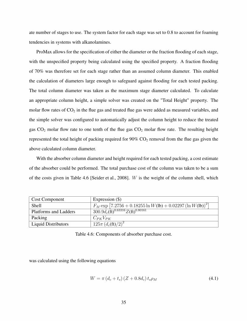
ate number of stages to use. The system factor for each stage was set to 0.8 to account for foaming

tendencies in systems with alkanolamines.

ProMax allows for the specification of either the diameter or the fraction flooding of each stage,

with the unspecified property being calculated using the specified property. A fraction flooding

of 70% was therefore set for each stage rather than an assumed column diameter. This enabled

the calculation of diameters large enough to safeguard against flooding for each tested packing.

The total column diameter was taken as the maximum stage diameter calculated. To calculate

an appropriate column height, a simple solver was created on the "Total Height" property. The

molar flow rates of CO2 in the flue gas and treated flue gas were added as measured variables, and

the simple solver was configured to automatically adjust the column height to reduce the treated

gas CO2 molar flow rate to one tenth of the flue gas CO2 molar flow rate. The resulting height

represented the total height of packing required for 90% CO2 removal from the flue gas given the

above calculated column diameter.

With the absorber column diameter and height required for each tested packing, a cost estimate

of the absorber could be performed. The total purchase cost of the column was taken to be a sum

of the costs given in Table 4.6 [Seider et al., 2008]. W is the weight of the column shell, which

Cost Component Expression ($)Shell FM exp

[7.2756 + 0.18255 lnW (lb) + 0.02297 (lnW (lb))2

]Platforms and Ladders 300.9dc(ft)0.63316Z(ft)0.80161

Packing CPKVPK

Liquid Distributors 125π (dc(ft)/2)2

Table 4.6: Components of absorber purchase cost.

was calculated using the following equations

W = π (dc + ts) (Z + 0.8dc) tsρM (4.1)

35

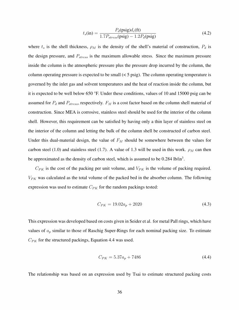
ts(in) =Pd(psig)dc(ft)

1.7Pstress(psig)− 1.2Pd(psig)(4.2)

where ts is the shell thickness, ρM is the density of the shell’s material of construction, Pd is

the design pressure, and Pstress is the maximum allowable stress. Since the maximum pressure

inside the column is the atmospheric pressure plus the pressure drop incurred by the column, the

column operating pressure is expected to be small (< 5 psig). The column operating temperature is

governed by the inlet gas and solvent temperatures and the heat of reaction inside the column, but

it is expected to be well below 650 °F. Under these conditions, values of 10 and 15000 psig can be

assumed for Pd and Pstress, respectively. FM is a cost factor based on the column shell material of

construction. Since MEA is corrosive, stainless steel should be used for the interior of the column

shell. However, this requirement can be satisfied by having only a thin layer of stainless steel on

the interior of the column and letting the bulk of the column shell be constructed of carbon steel.

Under this dual-material design, the value of FM should be somewhere between the values for

carbon steel (1.0) and stainless steel (1.7). A value of 1.3 will be used in this work. ρM can then

be approximated as the density of carbon steel, which is assumed to be 0.284 lb/in3.

CPK is the cost of the packing per unit volume, and VPK is the volume of packing required.

VPK was calculated as the total volume of the packed bed in the absorber column. The following

expression was used to estimate CPK for the random packings tested:

CPK = 19.02ap + 2020 (4.3)

This expression was developed based on costs given in Seider et al. for metal Pall rings, which have

values of ap similar to those of Raschig Super-Rings for each nominal packing size. To estimate

CPK for the structured packings, Equation 4.4 was used.

CPK = 5.37ap + 7486 (4.4)

The relationship was based on an expression used by Tsai to estimate structured packing costs

36

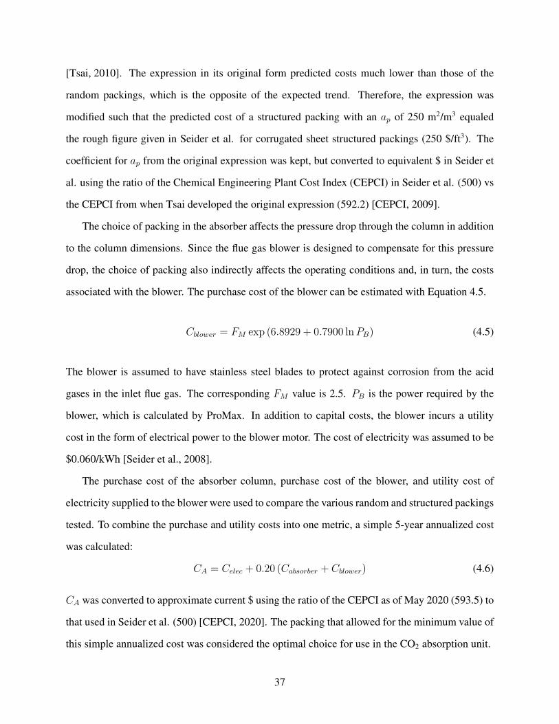
[Tsai, 2010]. The expression in its original form predicted costs much lower than those of the

random packings, which is the opposite of the expected trend. Therefore, the expression was

modified such that the predicted cost of a structured packing with an ap of 250 m2/m3 equaled

the rough figure given in Seider et al. for corrugated sheet structured packings (250 $/ft3). The

coefficient for ap from the original expression was kept, but converted to equivalent $ in Seider et

al. using the ratio of the Chemical Engineering Plant Cost Index (CEPCI) in Seider et al. (500) vs

the CEPCI from when Tsai developed the original expression (592.2) [CEPCI, 2009].

The choice of packing in the absorber affects the pressure drop through the column in addition

to the column dimensions. Since the flue gas blower is designed to compensate for this pressure

drop, the choice of packing also indirectly affects the operating conditions and, in turn, the costs

associated with the blower. The purchase cost of the blower can be estimated with Equation 4.5.

Cblower = FM exp (6.8929 + 0.7900 lnPB) (4.5)

The blower is assumed to have stainless steel blades to protect against corrosion from the acid

gases in the inlet flue gas. The corresponding FM value is 2.5. PB is the power required by the

blower, which is calculated by ProMax. In addition to capital costs, the blower incurs a utility

cost in the form of electrical power to the blower motor. The cost of electricity was assumed to be

$0.060/kWh [Seider et al., 2008].

The purchase cost of the absorber column, purchase cost of the blower, and utility cost of

electricity supplied to the blower were used to compare the various random and structured packings

tested. To combine the purchase and utility costs into one metric, a simple 5-year annualized cost

was calculated:

CA = Celec + 0.20 (Cabsorber + Cblower) (4.6)

CA was converted to approximate current $ using the ratio of the CEPCI as of May 2020 (593.5) to

that used in Seider et al. (500) [CEPCI, 2020]. The packing that allowed for the minimum value of

this simple annualized cost was considered the optimal choice for use in the CO2 absorption unit.

37

5. RESULTS AND DISCUSSION

5.1 Mass Transfer Correlation Development

5.1.1 Effective Interfacial Mass Transfer Area

Trends in the PSTC database were analyzed to determine which physical and packing prop-

erties should be included in the correlation developed for effective interfacial mass transfer area.

Figure 5.1 shows data points for the effective interfacial mass transfer area of Mellapak 250Y

plotted against the liquid superficial velocity for several superficial gas velocities. All physical

properties of the gas and liquid phases are held constant. The liquid superficial velocity clearly

Figure 5.1: Mellapak 250Y effective interfacial mass transfer area vs liquid superficial velocity fordifferent gas superficial velocities.

influences ae. Although the trend is slight, ae appears to increase with uG as well. In Figure 5.2,

ae is once again plotted against uL, but with a single value for uG and multiple liquid viscosities.

38

ae does not show a clear trend with respect to µL. However, ae appears to increase with surface

Figure 5.2: GT-OPTIM PAK 250Y effective interfacial mass transfer area vs liquid superficialvelocity for different liquid viscosities.

tension, as shown in Figure 5.3. In terms of packing parameters, ae appears to increase with the

corrugation angle in structured packing. As shown in Figure 5.4, GT-PAK 350Z, which has a cor-

rugation angle of 70°, has a consistently higher effective interfacial mass transfer area than that of

GT-PAK 350Y (α = 45) when all other physical and packing properties are held constant.

Based on the observed trends above, ae was taken to be a function of uG, uL, and σ. When

applied to structured packing, ae was also taken to be a function of α. To make the correlation

for ae dimensionless, the groups ReG, ReL, WeL, FrL, and cosαcosπ/4

were chosen for regression.

Additionally, a constant, CM , with different values for metal packings and plastic packings was

included to account for the effect of packing material of construction. The definitions for the

dimensionless parameters can be found in Chapter 1. FrL was included on the semi-theoretical

39

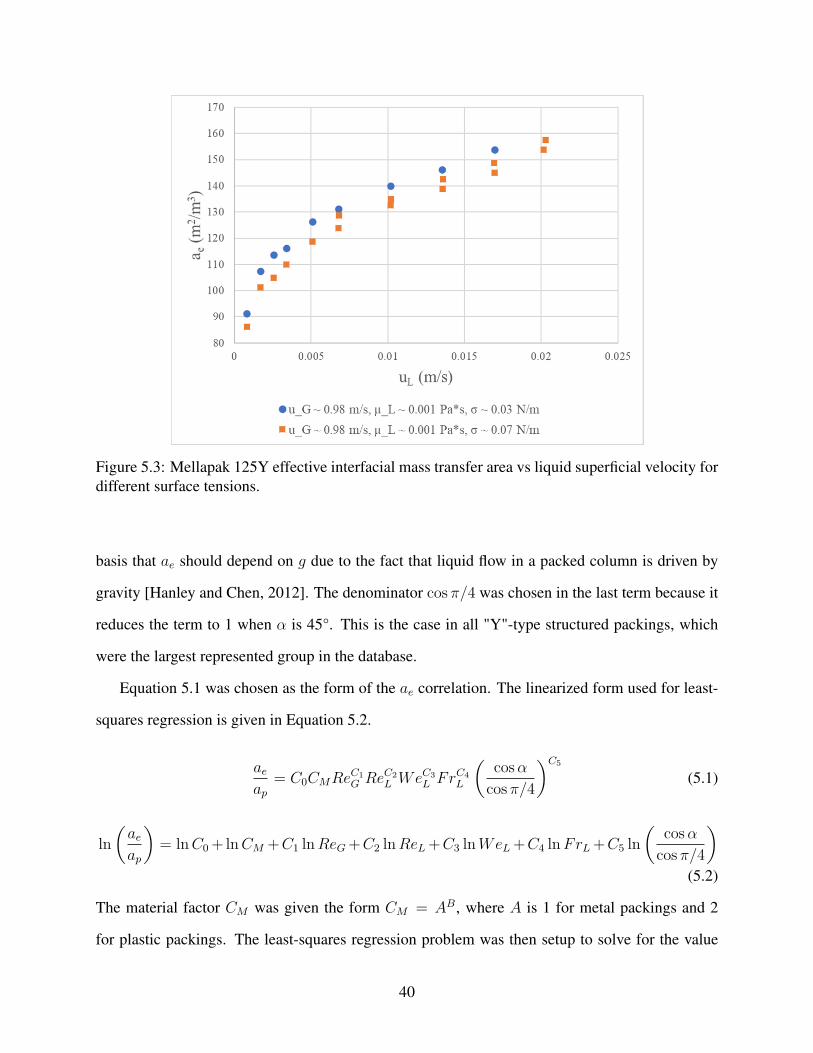
Figure 5.3: Mellapak 125Y effective interfacial mass transfer area vs liquid superficial velocity fordifferent surface tensions.

basis that ae should depend on g due to the fact that liquid flow in a packed column is driven by

gravity [Hanley and Chen, 2012]. The denominator cosπ/4 was chosen in the last term because it

reduces the term to 1 when α is 45°. This is the case in all "Y"-type structured packings, which

were the largest represented group in the database.

Equation 5.1 was chosen as the form of the ae correlation. The linearized form used for least-

squares regression is given in Equation 5.2.

aeap

= C0CMReC1G ReC2

L WeC3L FrC4

L

(cosα

cos π/4

)C5

(5.1)

ln

(aeap

)= lnC0+lnCM +C1 lnReG+C2 lnReL+C3 lnWeL+C4 lnFrL+C5 ln

(cosα

cos π/4

)(5.2)

The material factor CM was given the form CM = AB, where A is 1 for metal packings and 2

for plastic packings. The least-squares regression problem was then setup to solve for the value

40

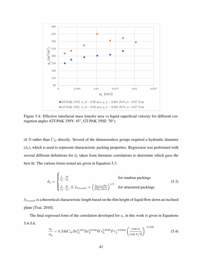
Figure 5.4: Effective interfacial mass transfer area vs liquid superficial velocity for different cor-rugation angles (GT-PAK 350Y: 45°, GT-PAK 350Z: 70°).

of B rather than CM directly. Several of the dimensionless groups required a hydraulic diameter

(dh), which is used to represent characteristic packing properties. Regression was performed with

several different definitions for dh taken from literature correlations to determine which gave the

best fit. The various forms tested are given in Equation 5.3.

dh =

1ap, 4εap

for random packings

1ap, 4εap, S, δNusselt =

(3µLuLBh4SρL sinα

)1/3

for structured packings(5.3)

δNusselt is a theoretical characteristic length based on the film height of liquid flow down an inclined

plane [Tsai, 2010].

The final regressed form of the correlation developed for ae in this work is given in Equations

5.4-5.6.aeap

= 0.346CMRe0.162G Re0.0156L We0.0709L Fr−0.0104L

(cosα

cos π/4

)−0.120

(5.4)

41

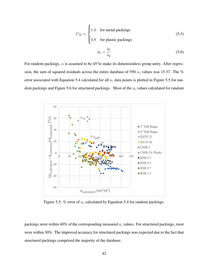
CM =

1.0 for metal packings

0.8 for plastic packings(5.5)

dh =4ε

ap(5.6)

For random packings, α is assumed to be 45°to make its dimensionless group unity. After regres-

sion, the sum of squared residuals across the entire database of 950 ae values was 15.37. The %

error associated with Equation 5.4 calculated for all ae data points is plotted in Figure 5.5 for ran-

dom packings and Figure 5.6 for structured packings. Most of the ae values calculated for random

Figure 5.5: % error of ae calculated by Equation 5.4 for random packings.

packings were within 40% of the corresponding measured ae values. For structured packings, most

were within 30%. The improved accuracy for structured packings was expected due to the fact that

structured packings comprised the majority of the database.

42

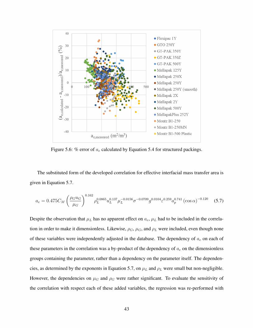
Figure 5.6: % error of ae calculated by Equation 5.4 for structured packings.

The substituted form of the developed correlation for effective interfacial mass transfer area is

given in Equation 5.7.

ae = 0.475CM

(ρGuG

µG

)0.162

ρ0.0865L u0.137L µ−0.0156

L σ−0.0709g0.0104ε0.259a0.741p (cosα)−0.120 (5.7)

Despite the observation that µL has no apparent effect on ae, µL had to be included in the correla-

tion in order to make it dimensionless. Likewise, ρG, µG, and ρL were included, even though none

of these variables were independently adjusted in the database. The dependency of ae on each of

these parameters in the correlation was a by-product of the dependency of ae on the dimensionless

groups containing the parameter, rather than a dependency on the parameter itself. The dependen-

cies, as determined by the exponents in Equation 5.7, on µL and ρL were small but non-negligible.

However, the dependencies on µG and ρG were rather significant. To evaluate the sensitivity of

the correlation with respect each of these added variables, the regression was re-performed with

43

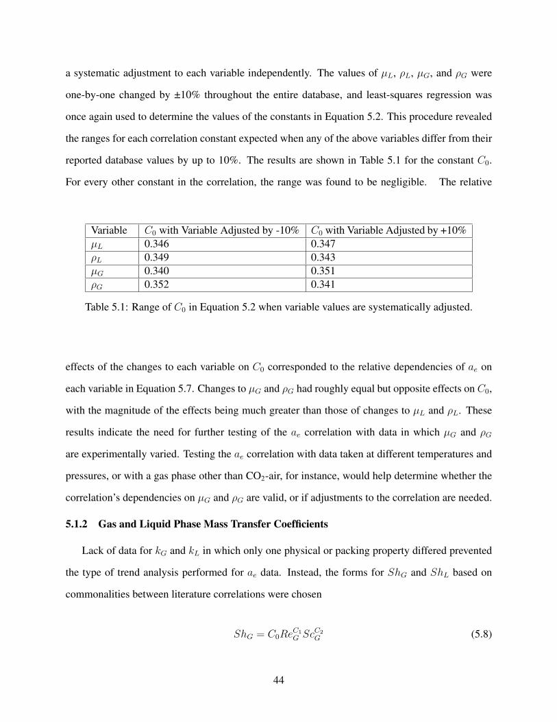
a systematic adjustment to each variable independently. The values of µL, ρL, µG, and ρG were

one-by-one changed by ±10% throughout the entire database, and least-squares regression was

once again used to determine the values of the constants in Equation 5.2. This procedure revealed

the ranges for each correlation constant expected when any of the above variables differ from their

reported database values by up to 10%. The results are shown in Table 5.1 for the constant C0.

For every other constant in the correlation, the range was found to be negligible. The relative

Variable C0 with Variable Adjusted by -10% C0 with Variable Adjusted by +10%µL 0.346 0.347ρL 0.349 0.343µG 0.340 0.351ρG 0.352 0.341

Table 5.1: Range of C0 in Equation 5.2 when variable values are systematically adjusted.

effects of the changes to each variable on C0 corresponded to the relative dependencies of ae on

each variable in Equation 5.7. Changes to µG and ρG had roughly equal but opposite effects on C0,

with the magnitude of the effects being much greater than those of changes to µL and ρL. These

results indicate the need for further testing of the ae correlation with data in which µG and ρG

are experimentally varied. Testing the ae correlation with data taken at different temperatures and

pressures, or with a gas phase other than CO2-air, for instance, would help determine whether the

correlation’s dependencies on µG and ρG are valid, or if adjustments to the correlation are needed.

5.1.2 Gas and Liquid Phase Mass Transfer Coefficients

Lack of data for kG and kL in which only one physical or packing property differed prevented

the type of trend analysis performed for ae data. Instead, the forms for ShG and ShL based on

commonalities between literature correlations were chosen

ShG = C0ReC1G ScC2

G (5.8)

44

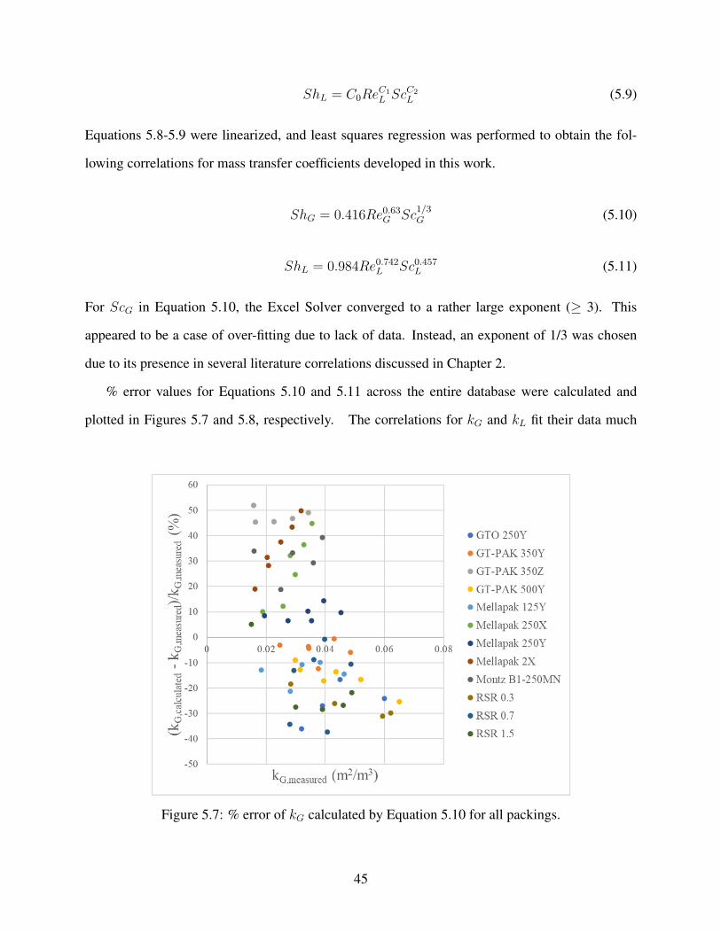
ShL = C0ReC1L ScC2

L (5.9)

Equations 5.8-5.9 were linearized, and least squares regression was performed to obtain the fol-

lowing correlations for mass transfer coefficients developed in this work.

ShG = 0.416Re0.63G Sc1/3G (5.10)

ShL = 0.984Re0.742L Sc0.457L (5.11)

For ScG in Equation 5.10, the Excel Solver converged to a rather large exponent (≥ 3). This

appeared to be a case of over-fitting due to lack of data. Instead, an exponent of 1/3 was chosen

due to its presence in several literature correlations discussed in Chapter 2.

% error values for Equations 5.10 and 5.11 across the entire database were calculated and

plotted in Figures 5.7 and 5.8, respectively. The correlations for kG and kL fit their data much

Figure 5.7: % error of kG calculated by Equation 5.10 for all packings.

45

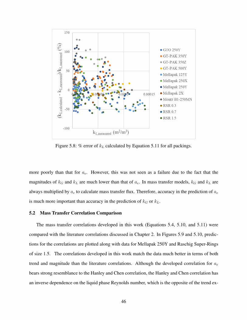
Figure 5.8: % error of kL calculated by Equation 5.11 for all packings.

more poorly than that for ae. However, this was not seen as a failure due to the fact that the

magnitudes of kG and kL are much lower than that of ae. In mass transfer models, kG and kL are

always multiplied by ae to calculate mass transfer flux. Therefore, accuracy in the prediction of ae

is much more important than accuracy in the prediction of kG or kL.

5.2 Mass Transfer Correlation Comparison

The mass transfer correlations developed in this work (Equations 5.4, 5.10, and 5.11) were

compared with the literature correlations discussed in Chapter 2. In Figures 5.9 and 5.10, predic-

tions for the correlations are plotted along with data for Mellapak 250Y and Raschig Super-Rings

of size 1.5. The correlations developed in this work match the data much better in terms of both

trend and magnitude than the literature correlations. Although the developed correlation for ae

bears strong resemblance to the Hanley and Chen correlation, the Hanley and Chen correlation has

an inverse dependence on the liquid phase Reynolds number, which is the opposite of the trend ex-

46

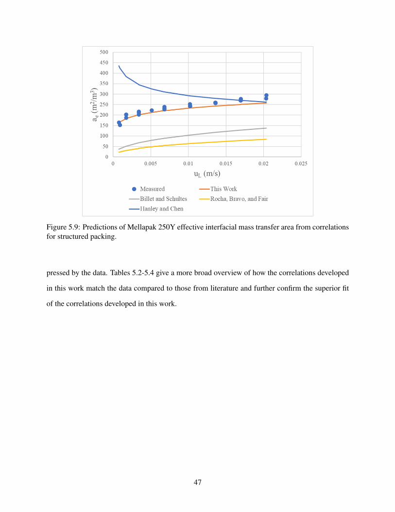
Figure 5.9: Predictions of Mellapak 250Y effective interfacial mass transfer area from correlationsfor structured packing.

pressed by the data. Tables 5.2-5.4 give a more broad overview of how the correlations developed

in this work match the data compared to those from literature and further confirm the superior fit

of the correlations developed in this work.

47

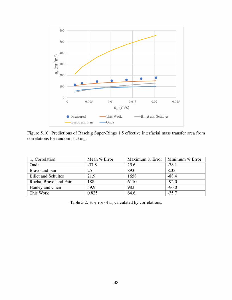
Figure 5.10: Predictions of Raschig Super-Rings 1.5 effective interfacial mass transfer area fromcorrelations for random packing.

ae Correlation Mean % Error Maximum % Error Minimum % ErrorOnda -37.8 25.6 -78.1Bravo and Fair 251 893 8.33Billet and Schultes 21.9 1658 -88.4Rocha, Bravo, and Fair 188 6110 -92.0Hanley and Chen 59.9 983 -96.0This Work 0.825 64.6 -35.7

Table 5.2: % error of ae calculated by correlations.

48

kG Correlation Mean % Error Maximum % Error Minimum % ErrorOnda 8.79 61.4 -19.7Billet and Schultes 62.0 151 -25.7Rocha, Bravo, and Fair -31.0 -0.704 -58.3Hanley and Chen -81.6 -63.7 -90.8This Work 3.20 51.8 -37.3

Table 5.3: % error of kG calculated by correlations.

kL Correlation Mean % Error Maximum % Error Minimum % ErrorOnda 40.3 233 -71.4Billet and Schultes 202 831 -46.3Rocha, Bravo, and Fair 230 1135 0.112Hanley and Chen -61.7 12.5 -97.6This Work 7.14 132 -59.9

Table 5.4: % error of kL calculated by correlations.

5.3 Design and Economic Analysis

Equations 5.4, 5.10, and 5.11 were implemented in ProMax as "User Defined" mass transfer

correlations (as discussed in Chapter 4) and used to test seven random and structured packings in

the ProMax CO2 absorber model. The results are shown in Tables 5.5-5.6. For all of the packings

tested, multiple absorber columns were required. This was due to the high flow rate of flue gas.

To keep fraction flooding below 70% in these circumstances, the diameter of each column had to

be large. When simulated as a single column, the absorber diameter calculated by ProMax was

greater than the required absorber height. This is an impractical design, so multiple columns in

parallel were instead assumed [Towler and Sinnott, 2013].

Raschig Super-Rings of size 1.5 are considered to be the optimum packing choice based on

this analysis. Despite the lower pressure drop and, in turn, blower purchase and utility costs as-

sociated with the structured packings, the purchase cost of the column dominated the annualized

cost, making the random packings generally more cost-effective than the structured packings.

49

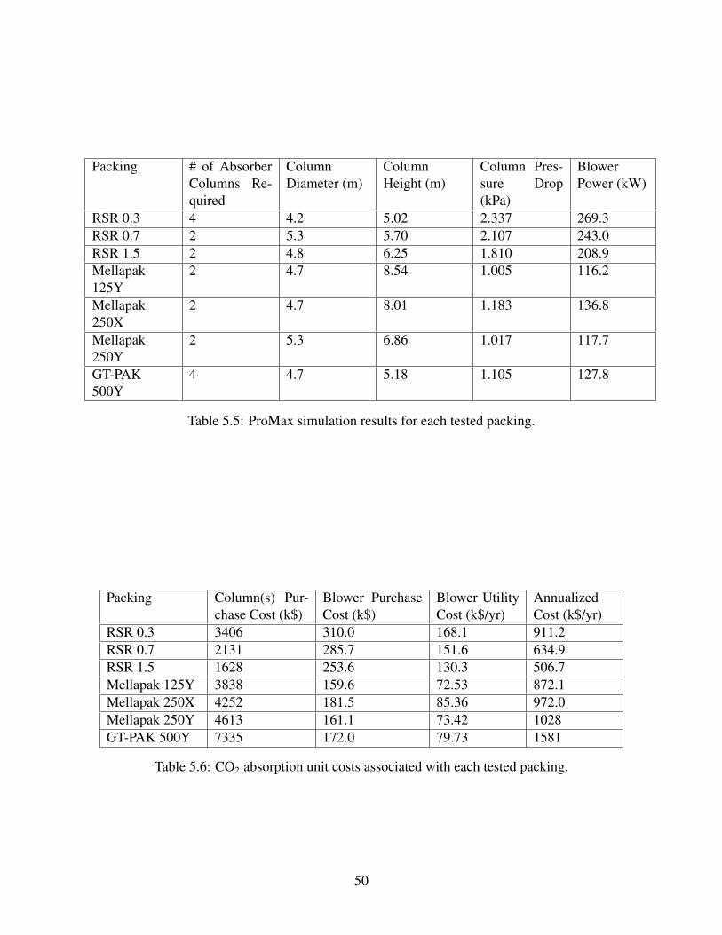
Packing # of AbsorberColumns Re-quired

ColumnDiameter (m)

ColumnHeight (m)

Column Pres-sure Drop(kPa)

BlowerPower (kW)

RSR 0.3 4 4.2 5.02 2.337 269.3RSR 0.7 2 5.3 5.70 2.107 243.0RSR 1.5 2 4.8 6.25 1.810 208.9Mellapak125Y

2 4.7 8.54 1.005 116.2

Mellapak250X

2 4.7 8.01 1.183 136.8

Mellapak250Y

2 5.3 6.86 1.017 117.7

GT-PAK500Y

4 4.7 5.18 1.105 127.8

Table 5.5: ProMax simulation results for each tested packing.

Packing Column(s) Pur-chase Cost (k$)

Blower PurchaseCost (k$)

Blower UtilityCost (k$/yr)

AnnualizedCost (k$/yr)

RSR 0.3 3406 310.0 168.1 911.2RSR 0.7 2131 285.7 151.6 634.9RSR 1.5 1628 253.6 130.3 506.7Mellapak 125Y 3838 159.6 72.53 872.1Mellapak 250X 4252 181.5 85.36 972.0Mellapak 250Y 4613 161.1 73.42 1028GT-PAK 500Y 7335 172.0 79.73 1581

Table 5.6: CO2 absorption unit costs associated with each tested packing.

50

6. CONCLUSIONS

New correlations for the effective interfacial mass transfer area, gas phase mass transfer co-

efficient, and liquid phase mass transfer coefficient in a packed column were developed. The

correlations were regressed using data published elsewhere for various types of random and struc-

tured packing encompassing ranges of gas and liquid superficial velocities, liquid viscosity, and

surface tension. The correlation for effective interfacial mass transfer area was developed with the

capacity to account for trends with respect to these parameters as well as several packing-specific

parameters, such as specific area, void fraction, material of construction, and corrugation angle

in structured packing. Overall, the correlations fit the data well, with accuracy in predicting the

magnitude and trends of data points exceeding that of literature correlations.

The new correlations were applied to modeling CO2 capture by incorporating them into the

process simulator ProMax and using ProMax to simulate a CO2 absorber column treating flue gas

from a 50MW coal-fired power plant. This study demonstrated use of the ProMax "User Defined"

mass transfer correlation feature, which can be used to customize the software’s mass and heat

transfer column models. Multiple packings were tested in the absorber, and an economic analysis

was used to determine that Raschig Super-Rings of size 1.5 were the optimal choice of packing

under the specified conditions.

Future work relevant to this study includes testing the correlations with additional data and

increasing the complexity of the CO2 absorber case study. The correlations developed in this work

are purely empirical and therefore may be significantly inaccurate outside of tested data regions.

Furthermore, the data did not include any systematic variation of the physical properties of the gas

phase, which makes dependencies on these variables in the correlation unsubstantiated. In terms

of the CO2 absorber case study, the economic analysis could be made more rigorous. Including

factors like capital depreciation could change the relative importance of utility versus capital costs,

which could change the conclusion of the study. Either of these measures would further this work’s

goal of developing and applying useful mass transfer correlations for CO2 capture modeling.

51

REFERENCES

[EPA, 2018] (2018). Sources of greenhouse gas emissions. https://www.epa.gov/ghgemissions/sources-greenhouse-gas-emissions.

[BRE, 2020a] (2020a). BRE-231: Sour Gas Processing: An Advanced Course on Removing Un-desirable Components from Gases and Liquids. Bryan Research and Engineering, LLC.

[EIA, 2020] (2020). Energy and the environment explained. https://www.eia.gov/energyexplained/energy-and-the-environment.

[BRE, 2020b] (2020b). ProMax Help v5.0. Bryan Research and Engineering, LLC.

[Aboudheir and McIntyre, 2009] Aboudheir, A. and McIntyre, G. (2009). Industrial design andoptimization of CO2 capture, dehydration, and compression facilities. Technical report, BryanResearch and Engineering, Inc.

[Billet and Schultes, 1993] Billet, R. and Schultes, M. (1993). Predicting mass transfer in packedcolumns. Chemical Engineering Technology, 16(1):1–9.

[Billet and Schultes, 1999] Billet, R. and Schultes, M. (1999). Prediction of mass transfer columnswith dumped and arranged packings: Updated summary of the calculation method of billet andschultes. Chemical Engineering Research and Design, 77(1):498–504.

[Bravo and Fair, 1982] Bravo, J. L. and Fair, J. R. (1982). Generalized correlation for mass trans-fer in packed distillation columns. Industrial and Engineering Chemistry Process Design andDevelopment, 21(1):162–170.

[CEPCI, 2009] CEPCI (2009). Economic indicators. Chemical Engineering, 116(2):64.

[CEPCI, 2020] CEPCI (2020). Economic indicators. Chemical Engineering, 127(9):72.

[Green and Perry, 2008] Green, D. W. and Perry, R. H. (2008). Perry’s Chemical Engineers’Handbook, 8th Edition. McGraw-Hill Professional.

[Hanley and Chen, 2012] Hanley, B. and Chen, C.-C. (2012). New mass-transfer correlations forpacked towers. AIChE Journal, 58(1):132–152.

52

[Incropera et al., 2007] Incropera, F. P., DeWitt, D. P., Bergman, T. L., and Lavine, A. S. (2007).Fundamentals of Heat and Mass Transfer, 6th Edition. Wiley.

[Kister, 1992] Kister, H. Z. (1992). Distillation Design. McGraw-Hill Education.

[Olujic et al., 2001] Olujic, Z., Jansen, H., Kaibel, B., Rietfort, T., and Zich, E. (2001). Stretch-ing the capacity of structured packings. Industrial and Engineering Chemistry Research,40(26):6172–6180.

[Onda et al., 1968] Onda, K., Takeuchi, H., and Okumoto, Y. (1968). Mass transfer coefficientsbetween gas and liquid phases in packed columns. Journal of Chemical Engineering of Japan,1(1):56–62.

[Rao and Rubin, 2002] Rao, A. B. and Rubin, E. S. (2002). A technical, economic, and envi-ronmental assessment of amine-based CO2 capture technology for power plant greenhouse gascontrol. Environmental Science and Technology, 36(20):4467–4475.

[Rocha et al., 1993] Rocha, J. A., Bravo, J. L., and Fair, J. R. (1993). Distillation columns contain-ing structured packings: A comprehensive model for their performance. 1. hydraulic models.Industrial and Engineering Chemistry Research, 32(4):641–651.

[Rocha et al., 1996] Rocha, J. A., Bravo, J. L., and Fair, J. R. (1996). Distillation columns con-taining structured packings: A comprehensive model for their performance. 2. mass-transfermodel. Industrial and Engineering Chemistry Research, 35(5):641–651.

[Seider et al., 2008] Seider, W., Seader, J., Lewin, D., and Widagdo, S. (2008). Product andProcess Design Principles: Synthesis, Analysis, and Evaluation, 3rd Edition. Wiley.

[Skowlund et al., 2012] Skowlund, C., Hlavinka, M., Lopez, M., and Fitz, C. (2012). Comparisonof ideal stage and mass transfer models for separation processes with and without chemicalreactions. Technical report, Bryan Research and Engineering, Inc.

[Song, 2017] Song, D. (2017). Effect of Liquid Viscosity on Liquid Film Mass Transfer for Pack-ings. PhD thesis, University of Texas at Austin.

[Towler and Sinnott, 2013] Towler, G. and Sinnott, R. (2013). Chemical Engineering Design:Principles, Practice and Economics of Plant and Process Design, 2nd Edition. Butterworth-Heinemann.

[Tsai, 2010] Tsai, R. (2010). Mass Transfer Area of Structured Packing. PhD thesis, Universityof Texas at Austin.

53

[Wang, 2015] Wang, C. (2015). Mass Transfer Coefficients and Effective Area of Packing. PhDthesis, University of Texas at Austin.

[Wang et al., 2016] Wang, C., Song, D., Seibert, F., and Rochelle, G. (2016). Dimensionlessmodels for predicting the effective area, liquid-film, and gas-film mass-transfer coefficients ofpacking. Industrial and Engineering Chemistry Research, 55(18):5373–5384.

[Wilson, 2004] Wilson, I. (2004). Gas-liquid contact area of random and structured packing. Mas-ter’s thesis, University of Texas at Austin.

54

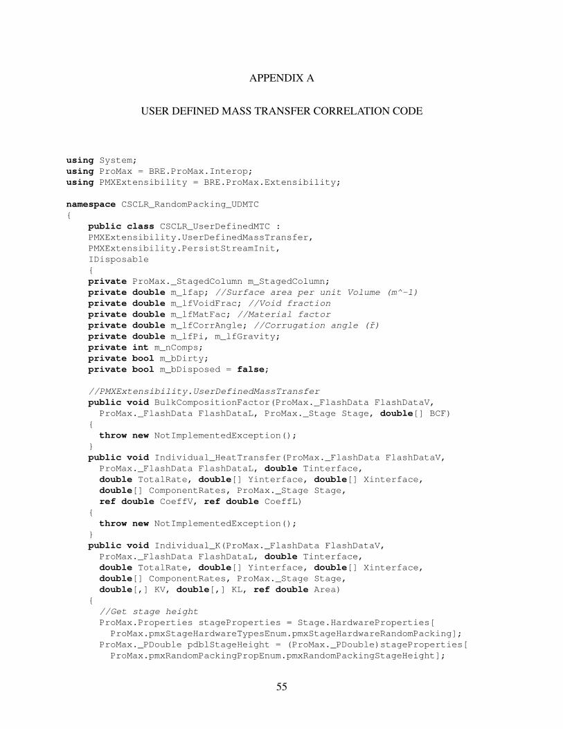
APPENDIX A

USER DEFINED MASS TRANSFER CORRELATION CODE

using System;using ProMax = BRE.ProMax.Interop;using PMXExtensibility = BRE.ProMax.Extensibility;

namespace CSCLR_RandomPacking_UDMTC{

public class CSCLR_UserDefinedMTC :PMXExtensibility.UserDefinedMassTransfer,PMXExtensibility.PersistStreamInit,IDisposable{private ProMax._StagedColumn m_StagedColumn;private double m_lfap; //Surface area per unit Volume (m^-1)private double m_lfVoidFrac; //Void fractionprivate double m_lfMatFac; //Material factorprivate double m_lfCorrAngle; //Corrugation angle (r)private double m_lfPi, m_lfGravity;private int m_nComps;private bool m_bDirty;private bool m_bDisposed = false;

//PMXExtensibility.UserDefinedMassTransferpublic void BulkCompositionFactor(ProMax._FlashData FlashDataV,

ProMax._FlashData FlashDataL, ProMax._Stage Stage, double[] BCF){

throw new NotImplementedException();}public void Individual_HeatTransfer(ProMax._FlashData FlashDataV,

ProMax._FlashData FlashDataL, double Tinterface,double TotalRate, double[] Yinterface, double[] Xinterface,double[] ComponentRates, ProMax._Stage Stage,ref double CoeffV, ref double CoeffL)

{throw new NotImplementedException();

}public void Individual_K(ProMax._FlashData FlashDataV,

ProMax._FlashData FlashDataL, double Tinterface,double TotalRate, double[] Yinterface, double[] Xinterface,double[] ComponentRates, ProMax._Stage Stage,double[,] KV, double[,] KL, ref double Area)

{//Get stage heightProMax.Properties stageProperties = Stage.HardwareProperties[

ProMax.pmxStageHardwareTypesEnum.pmxStageHardwareRandomPacking];ProMax._PDouble pdblStageHeight = (ProMax._PDouble)stageProperties[

ProMax.pmxRandomPackingPropEnum.pmxRandomPackingStageHeight];

55

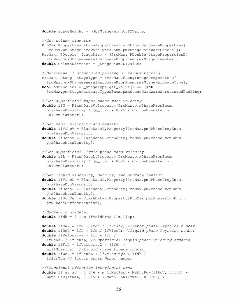
double stageHeight = pdblStageHeight.SIValue;

//Get column diameterProMax.Properties stagePropertiesD = Stage.HardwareProperties[

ProMax.pmxStageHardwareTypesEnum.pmxStageHardwareGeneral];ProMax._PDouble _StageDiam = (ProMax._PDouble)stagePropertiesD[

ProMax.pmxStageGeneralHardwarePropEnum.pmxStageDiameter];double ColumnDiameter = _StageDiam.SIValue;

//Determine if structured packing or random packingProMax._PLong _StageType = (ProMax.PLong)stagePropertiesD[

ProMax.pmxStageGeneralHardwarePropEnum.pmxStageHardwareType];bool bStrucPack = _StageType.get_Value() == (int)

ProMax.pmxStageHardwareTypesEnum.pmxStageHardwareStructuredPacking;

//Get superficial vapor phase mass velocitydouble lfG = FlashDataV.Property[ProMax.pmxPhasePropEnum.

pmxPhaseMassFlow] / (m_lfPi * 0.25 * ColumnDiameter *ColumnDiameter);

//Get vapor viscosity and densitydouble lfViscV = FlashDataV.Property[ProMax.pmxPhasePropEnum.

pmxPhaseDynViscosity];double lfDensV = FlashDataV.Property[ProMax.pmxPhasePropEnum.

pmxPhaseMassDensity];

//Get superficial liquid phase mass velocitydouble lfL = FlashDataL.Property[ProMax.pmxPhasePropEnum.

pmxPhaseMassFlow] / (m_lfPi * 0.25 * ColumnDiameter *ColumnDiameter);

//Get liquid viscosity, density, and surface tensiondouble lfViscL = FlashDataL.Property[ProMax.pmxPhasePropEnum.

pmxPhaseDynViscosity];double lfDensL = FlashDataL.Property[ProMax.pmxPhasePropEnum.

pmxPhaseMassDensity];double lfSurTen = FlashDataL.Property[ProMax.pmxPhasePropEnum.

pmxPhaseSurfaceTension];

//Hydraulic diameterdouble lfdh = 4 * m_lfVoidFrac / m_lfap;

double lfReV = lfG * lfdh / lfViscV; //Vapor phase Reynolds numberdouble lfReL = lfL * lfdh/ lfViscL; //Liquid phase Reynolds numberdouble lfVelocity2 = lfL * lfL /

lfDensL / lfDensL; //Superficial liquid phase velocity squareddouble lfFrL = lfVelocity2 / (lfdh *

m_lfGravity); //Liquid phase Froude numberdouble lfWeL = lfDensL * lfVelocity2 * lfdh /

lfSurTen;// Liquid phase Weber number

//Fractional effective interfacial areadouble lf_ae_ap = 0.346 * m_lfMatFac * Math.Pow(lfReV, 0.162) *

Math.Pow(lfReL, 0.0156) * Math.Pow(lfWeL, 0.0709) *

56

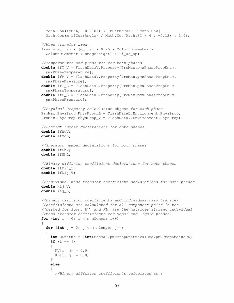
Math.Pow(lfFrL, -0.0104) * (bStrucPack ? Math.Pow(Math.Cos(m_lfCorrAngle) / Math.Cos(Math.PI / 4), -0.12) : 1.0);

//Mass transfer areaArea = m_lfap * (m_lfPi * 0.25 * ColumnDiameter *

ColumnDiameter * stageHeight) * lf_ae_ap;

//Temperatures and pressures for both phasesdouble lfT_V = FlashDataV.Property[ProMax.pmxPhasePropEnum.

pmxPhaseTemperature];double lfP_V = FlashDataV.Property[ProMax.pmxPhasePropEnum.

pmxPhasePressure];double lfT_L = FlashDataL.Property[ProMax.pmxPhasePropEnum.

pmxPhaseTemperature];double lfP_L = FlashDataL.Property[ProMax.pmxPhasePropEnum.

pmxPhasePressure];

//Physical Property calculation object for each phaseProMax.PhysProp PhysProp_L = FlashDataL.Environment.PhysProp;ProMax.PhysProp PhysProp_V = FlashDataV.Environment.PhysProp;

//Schmidt number declarations for both phasesdouble lfScV;double lfScL;

//Sherwood number declarations for both phasesdouble lfShV;double lfShL;

//Binary diffusion coefficient declarations for both phasesdouble lfDij_L;double lfDij_V;

//Individual mass transfer coefficient declarations for both phasesdouble kij_V;double kij_L;

//Binary diffusion coefficients and individual mass transfer//coefficients are calculated for all component pairs in the//nested for loop. KV_ and KL_ are the matrices storing individual//mass transfer coefficients for vapor and liquid phases.for (int i = 0; i < m_nComps; i++){

for (int j = 0; j < m_nComps; j++){

int uStatus = (int)ProMax.pmxPropStatusValues.pmxPropStatusOK;if (i == j){

KV[i, j] = 0.0;KL[i, j] = 0.0;

}else{

//Binary diffusion coefficients calculated as a

57

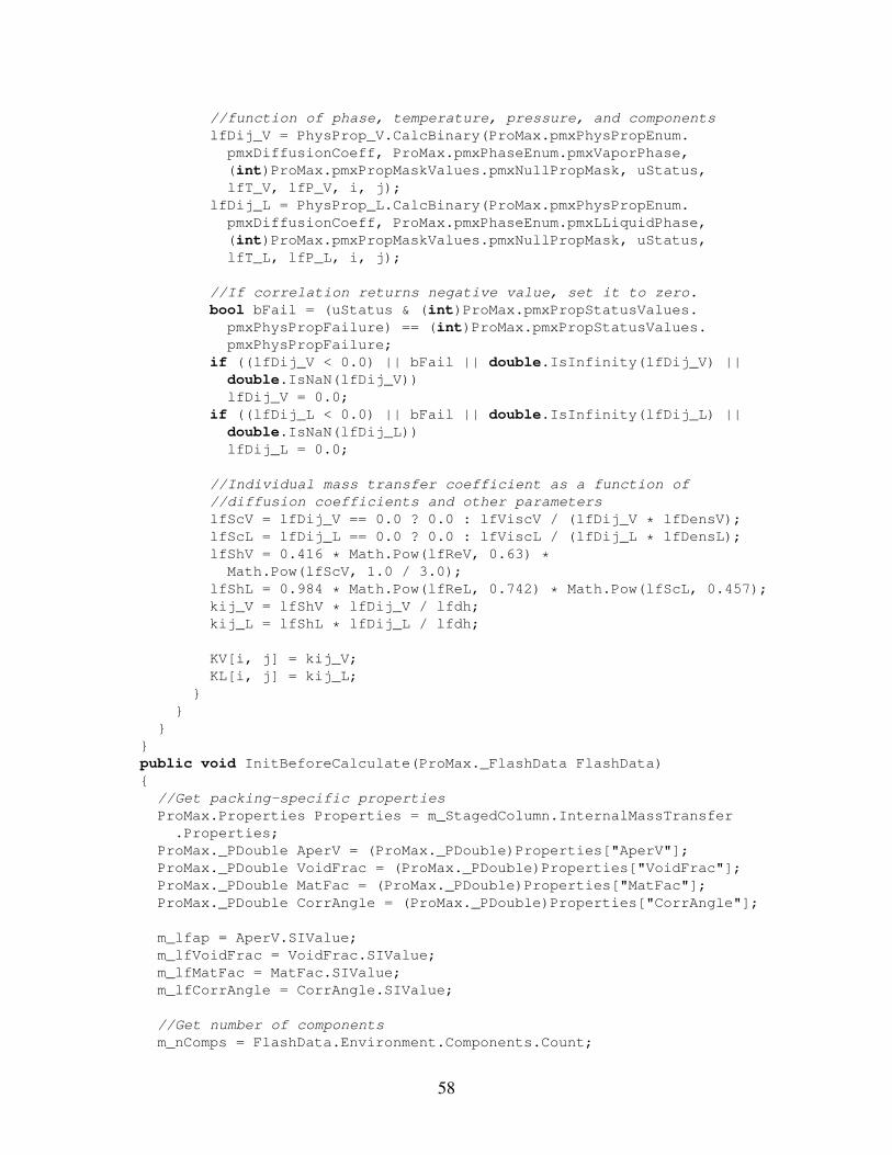
//function of phase, temperature, pressure, and componentslfDij_V = PhysProp_V.CalcBinary(ProMax.pmxPhysPropEnum.

pmxDiffusionCoeff, ProMax.pmxPhaseEnum.pmxVaporPhase,(int)ProMax.pmxPropMaskValues.pmxNullPropMask, uStatus,lfT_V, lfP_V, i, j);

lfDij_L = PhysProp_L.CalcBinary(ProMax.pmxPhysPropEnum.pmxDiffusionCoeff, ProMax.pmxPhaseEnum.pmxLLiquidPhase,(int)ProMax.pmxPropMaskValues.pmxNullPropMask, uStatus,lfT_L, lfP_L, i, j);

//If correlation returns negative value, set it to zero.bool bFail = (uStatus & (int)ProMax.pmxPropStatusValues.

pmxPhysPropFailure) == (int)ProMax.pmxPropStatusValues.pmxPhysPropFailure;

if ((lfDij_V < 0.0) || bFail || double.IsInfinity(lfDij_V) ||double.IsNaN(lfDij_V))lfDij_V = 0.0;

if ((lfDij_L < 0.0) || bFail || double.IsInfinity(lfDij_L) ||double.IsNaN(lfDij_L))lfDij_L = 0.0;

//Individual mass transfer coefficient as a function of//diffusion coefficients and other parameterslfScV = lfDij_V == 0.0 ? 0.0 : lfViscV / (lfDij_V * lfDensV);lfScL = lfDij_L == 0.0 ? 0.0 : lfViscL / (lfDij_L * lfDensL);lfShV = 0.416 * Math.Pow(lfReV, 0.63) *

Math.Pow(lfScV, 1.0 / 3.0);lfShL = 0.984 * Math.Pow(lfReL, 0.742) * Math.Pow(lfScL, 0.457);kij_V = lfShV * lfDij_V / lfdh;kij_L = lfShL * lfDij_L / lfdh;

KV[i, j] = kij_V;KL[i, j] = kij_L;

}}

}}public void InitBeforeCalculate(ProMax._FlashData FlashData){

//Get packing-specific propertiesProMax.Properties Properties = m_StagedColumn.InternalMassTransfer

.Properties;ProMax._PDouble AperV = (ProMax._PDouble)Properties["AperV"];ProMax._PDouble VoidFrac = (ProMax._PDouble)Properties["VoidFrac"];ProMax._PDouble MatFac = (ProMax._PDouble)Properties["MatFac"];ProMax._PDouble CorrAngle = (ProMax._PDouble)Properties["CorrAngle"];

m_lfap = AperV.SIValue;m_lfVoidFrac = VoidFrac.SIValue;m_lfMatFac = MatFac.SIValue;m_lfCorrAngle = CorrAngle.SIValue;

//Get number of componentsm_nComps = FlashData.Environment.Components.Count;

58

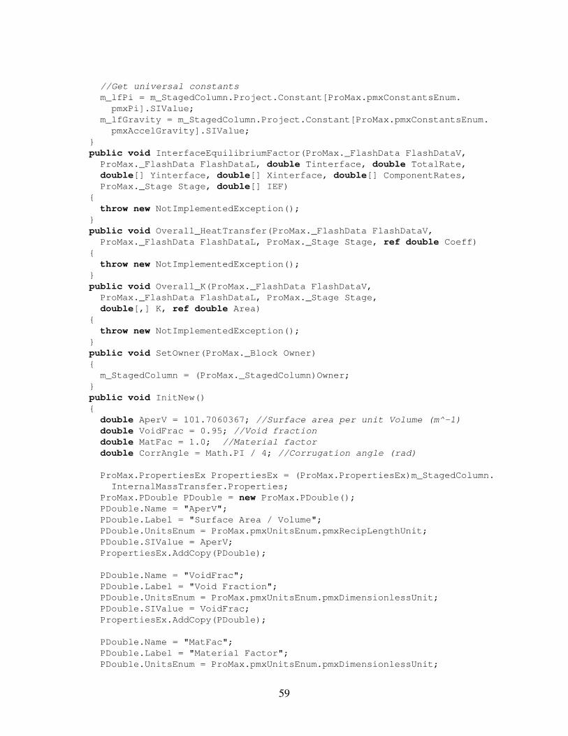
//Get universal constantsm_lfPi = m_StagedColumn.Project.Constant[ProMax.pmxConstantsEnum.

pmxPi].SIValue;m_lfGravity = m_StagedColumn.Project.Constant[ProMax.pmxConstantsEnum.

pmxAccelGravity].SIValue;}public void InterfaceEquilibriumFactor(ProMax._FlashData FlashDataV,

ProMax._FlashData FlashDataL, double Tinterface, double TotalRate,double[] Yinterface, double[] Xinterface, double[] ComponentRates,ProMax._Stage Stage, double[] IEF)

{throw new NotImplementedException();

}public void Overall_HeatTransfer(ProMax._FlashData FlashDataV,

ProMax._FlashData FlashDataL, ProMax._Stage Stage, ref double Coeff){

throw new NotImplementedException();}public void Overall_K(ProMax._FlashData FlashDataV,

ProMax._FlashData FlashDataL, ProMax._Stage Stage,double[,] K, ref double Area)

{throw new NotImplementedException();

}public void SetOwner(ProMax._Block Owner){

m_StagedColumn = (ProMax._StagedColumn)Owner;}public void InitNew(){

double AperV = 101.7060367; //Surface area per unit Volume (m^-1)double VoidFrac = 0.95; //Void fractiondouble MatFac = 1.0; //Material factordouble CorrAngle = Math.PI / 4; //Corrugation angle (rad)

ProMax.PropertiesEx PropertiesEx = (ProMax.PropertiesEx)m_StagedColumn.InternalMassTransfer.Properties;

ProMax.PDouble PDouble = new ProMax.PDouble();PDouble.Name = "AperV";PDouble.Label = "Surface Area / Volume";PDouble.UnitsEnum = ProMax.pmxUnitsEnum.pmxRecipLengthUnit;PDouble.SIValue = AperV;PropertiesEx.AddCopy(PDouble);

PDouble.Name = "VoidFrac";PDouble.Label = "Void Fraction";PDouble.UnitsEnum = ProMax.pmxUnitsEnum.pmxDimensionlessUnit;PDouble.SIValue = VoidFrac;PropertiesEx.AddCopy(PDouble);

PDouble.Name = "MatFac";PDouble.Label = "Material Factor";PDouble.UnitsEnum = ProMax.pmxUnitsEnum.pmxDimensionlessUnit;

59

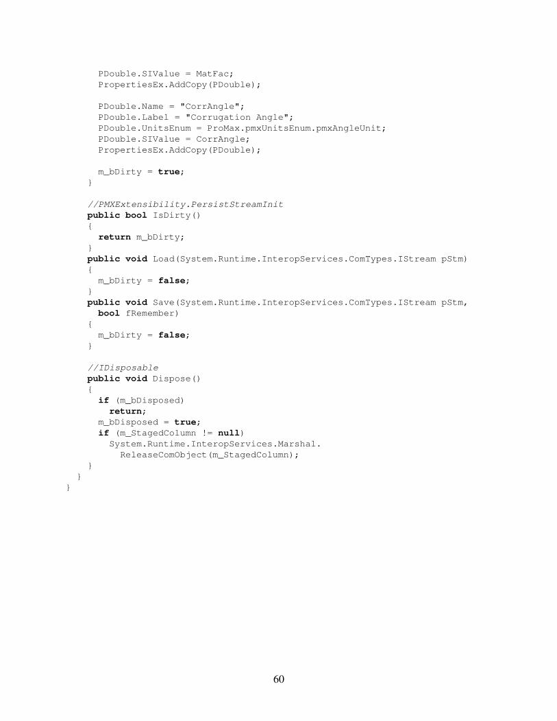
PDouble.SIValue = MatFac;PropertiesEx.AddCopy(PDouble);

PDouble.Name = "CorrAngle";PDouble.Label = "Corrugation Angle";PDouble.UnitsEnum = ProMax.pmxUnitsEnum.pmxAngleUnit;PDouble.SIValue = CorrAngle;PropertiesEx.AddCopy(PDouble);

m_bDirty = true;}

//PMXExtensibility.PersistStreamInitpublic bool IsDirty(){

return m_bDirty;}public void Load(System.Runtime.InteropServices.ComTypes.IStream pStm){

m_bDirty = false;}public void Save(System.Runtime.InteropServices.ComTypes.IStream pStm,

bool fRemember){

m_bDirty = false;}

//IDisposablepublic void Dispose(){

if (m_bDisposed)return;

m_bDisposed = true;if (m_StagedColumn != null)

System.Runtime.InteropServices.Marshal.ReleaseComObject(m_StagedColumn);

}}

}

60

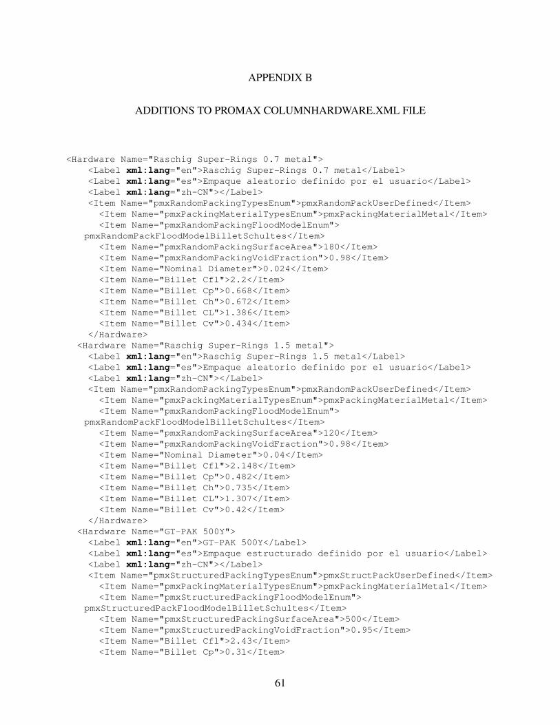
APPENDIX B

ADDITIONS TO PROMAX COLUMNHARDWARE.XML FILE

<Hardware Name="Raschig Super-Rings 0.7 metal"><Label xml:lang="en">Raschig Super-Rings 0.7 metal</Label><Label xml:lang="es">Empaque aleatorio definido por el usuario</Label><Label xml:lang="zh-CN"></Label><Item Name="pmxRandomPackingTypesEnum">pmxRandomPackUserDefined</Item>

<Item Name="pmxPackingMaterialTypesEnum">pmxPackingMaterialMetal</Item><Item Name="pmxRandomPackingFloodModelEnum">

pmxRandomPackFloodModelBilletSchultes</Item><Item Name="pmxRandomPackingSurfaceArea">180</Item><Item Name="pmxRandomPackingVoidFraction">0.98</Item><Item Name="Nominal Diameter">0.024</Item><Item Name="Billet Cfl">2.2</Item><Item Name="Billet Cp">0.668</Item><Item Name="Billet Ch">0.672</Item><Item Name="Billet CL">1.386</Item><Item Name="Billet Cv">0.434</Item>

</Hardware><Hardware Name="Raschig Super-Rings 1.5 metal">

<Label xml:lang="en">Raschig Super-Rings 1.5 metal</Label><Label xml:lang="es">Empaque aleatorio definido por el usuario</Label><Label xml:lang="zh-CN"></Label><Item Name="pmxRandomPackingTypesEnum">pmxRandomPackUserDefined</Item>

<Item Name="pmxPackingMaterialTypesEnum">pmxPackingMaterialMetal</Item><Item Name="pmxRandomPackingFloodModelEnum">

pmxRandomPackFloodModelBilletSchultes</Item><Item Name="pmxRandomPackingSurfaceArea">120</Item><Item Name="pmxRandomPackingVoidFraction">0.98</Item><Item Name="Nominal Diameter">0.04</Item><Item Name="Billet Cfl">2.148</Item><Item Name="Billet Cp">0.482</Item><Item Name="Billet Ch">0.735</Item><Item Name="Billet CL">1.307</Item><Item Name="Billet Cv">0.42</Item>

</Hardware><Hardware Name="GT-PAK 500Y">

<Label xml:lang="en">GT-PAK 500Y</Label><Label xml:lang="es">Empaque estructurado definido por el usuario</Label><Label xml:lang="zh-CN"></Label><Item Name="pmxStructuredPackingTypesEnum">pmxStructPackUserDefined</Item>

<Item Name="pmxPackingMaterialTypesEnum">pmxPackingMaterialMetal</Item><Item Name="pmxStructuredPackingFloodModelEnum">

pmxStructuredPackFloodModelBilletSchultes</Item><Item Name="pmxStructuredPackingSurfaceArea">500</Item><Item Name="pmxStructuredPackingVoidFraction">0.95</Item><Item Name="Billet Cfl">2.43</Item><Item Name="Billet Cp">0.31</Item>

61

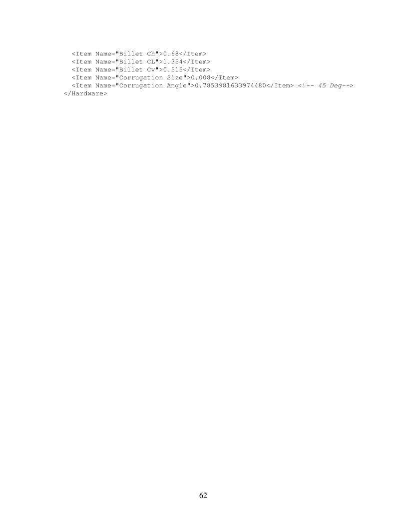
<Item Name="Billet Ch">0.68</Item><Item Name="Billet CL">1.354</Item><Item Name="Billet Cv">0.515</Item><Item Name="Corrugation Size">0.008</Item><Item Name="Corrugation Angle">0.7853981633974480</Item> <!-- 45 Deg-->

</Hardware>

62