UNIVERSITY OF HAWNI LIBRARY

MASS TRANSFER LIMITS TO NUTRIENT UPTAKE BY SHALLOW CORAL

REEF COMMUNITIES

A DISSERTATION SUBMITTED TO THE GRADUATE DIVISION OF THEUNIVERSITY OF HAWAI'I IN PARTIAL FULFILLMENT OF THE

REQUIREMENTS FOR THE DEGREE OF

DOCTOR OF PHILOSOPHY

IN

OCEANOGRAPHY

DECEMBER 2002

ByJames L. Falter

Dissertation Committee:

Marlin J. Atkinson, ChairpersonCarlos F.M. CoimbraMark A. MenifieldFrancis J. SansoneStephen V. Smith

© Copyright (2002)

by

James L. Falter

llJ

ACKNOWLEDGEMENTS

I would like to thank my committee for all of their assistance and interaction; it

was clear they were looking out for my best interests. Mahalo nui to Jim Fleming, who

as an unofficial committee member and mentor, showed me how to work with my hands.

His assistance in the field and in the construction of various experimental apparati (often

without the benefit of calculus) was fundamental to the completion of this degree. I

would like to thank Eric Hochberg for his support as a friend, sounding board, field

assistant, and international dive guide. I would also like to thank Dan Hoover, Jennifer

Liebeler, Janie Culp, and Ann Tarrant for the moral support that is essential for any

graduate student to succeed. I would like to thank Kimball Millikan, Philippe Barrault,

Serge Andrefouet, Kim Anthony, and Ken Longenecker for assistance with field

experiments and/or data analysis. Mahalo to Mark Merrifield for loaning me his

pressure sensors, and to Jerome Aucan for showing me how to use them as well as

running the SWAN simulations. Fenny Cox generously supplied me with nutrient data

for Kaneohe Bay. Additional thanks must be paid to Kathy Kozuma and Nancy Koike

who helped me struggle through the bureaucracy of the University and the degree

process. A warm aloha to my mother who supported my pursuit of this degree, despite

having to do it several thousands miles from home. This research was supported by

grants from Hawaii Sea Grant, the Biosphere II FoundationlCoumbia University, and the

National Science Foundation.

This dissertation belongs in part to my father, who taught me how to think.

iv

ABSTRACT

Uptake and assimilation of nutrients is essential to the productivity of coral reefs.

Nutrient uptake rates by coral reef communities have been hypothesized to be limited by

rates of mass transfer across a concentration boundary layer. The mass transfer

coefficient S (m dai l) relates the maximum nutrient flux allowed by mass transfer to the

nutrient concentration in the ambient water (Jmax =S[N]). The goal of this dissertation

is to determine the maximum rate at which a coral reef flat community can take up

nutrients according to mass transfer theory. Nutrient mass transfer coefficients for a

Kaneohe Bay Barrier Reef flat community were determined two ways. In the first

method, S was estimated from in situ measurements of wave-driven flow speeds (U h =

0.08-0.22 m S·I) and the friction coefficient of the reef flat (Cf = 0.22±O.03) using a mass

transfer correlation. S calculated from this method was 5.8±O.8 m dai l for phosphate

and 9.7±1.3 m dai l for nitrate and ammonium. The second method compared the

dissolution of artificial plaster forms (surface area = 0.1-1.0 m2) of varying roughness

scale (0.001-0.1 m) under wave-driven and steady flows (Uh = 0.02-0.21 m S·I). Results

showed 1) rates of mass transfer were linearly proportional to surface area regardless of

roughness scale and flow conditions, and 2) rates of mass transfer were 1.4-2.0 times

higher under wave-driven flows (-8-s in period) than under steady flows. Using

appropriate surface areas from the plaster dissolution experiments, S for the reef flat

community was 7±3 m da/ for phosphate and 12±5 m da/ for nitrate and ammonium.

Using the wave enhancement obtained from the plaster dissolution experiments, S could

be as high as 9.3±1.3 m day·1 and 15.5±2.1 m dai l. The phosphate uptake rate

coefficient from flow respirometry for the same reef flat community was 4.5-9 m dai l.

v

Thus, rates of phosphate uptake by the this community are at the limits of mass transfer.

Scaling maximum phosphate uptake rates by the average C:P of benthic autotrophic

tissue indicates that net primary production within this community is limited by nutrient

uptake.

vi

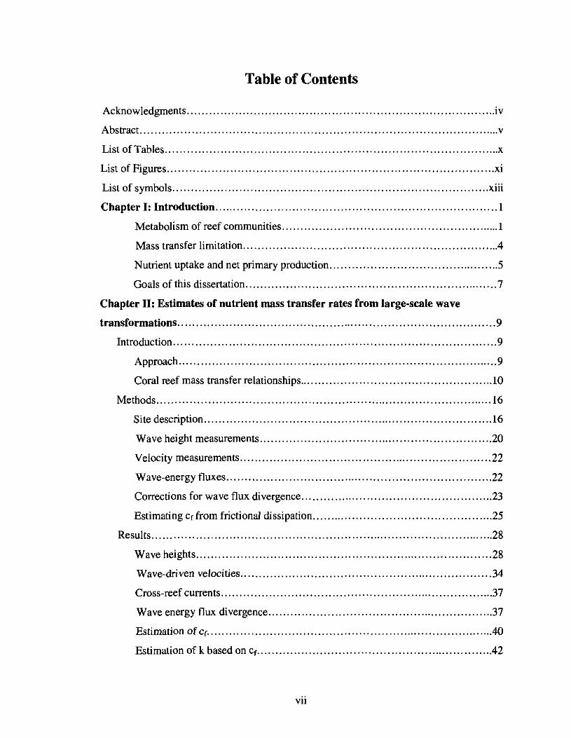
Table of Contents

Acknowledgments iv

Abstract v

List of Tables x

List of Figures xi

List of symbols xiii

Chapter I: Introduction l

Metabolism of reef communities 1

Mass transfer limitation .4

Nutrient uptake and net primary production 5

Goals of this dissertation 7

Chapter II: Estimates of nutrient mass transfer rates from large-scale wave

transformations 9

Introduction 9

Approach 9

Coral reef mass transfer relationships 10

Methods 16

Site description 16

Wave height measurements 20

Velocity measurements 22

Wave-energy fluxes 22

Corrections for wave flux divergence 23

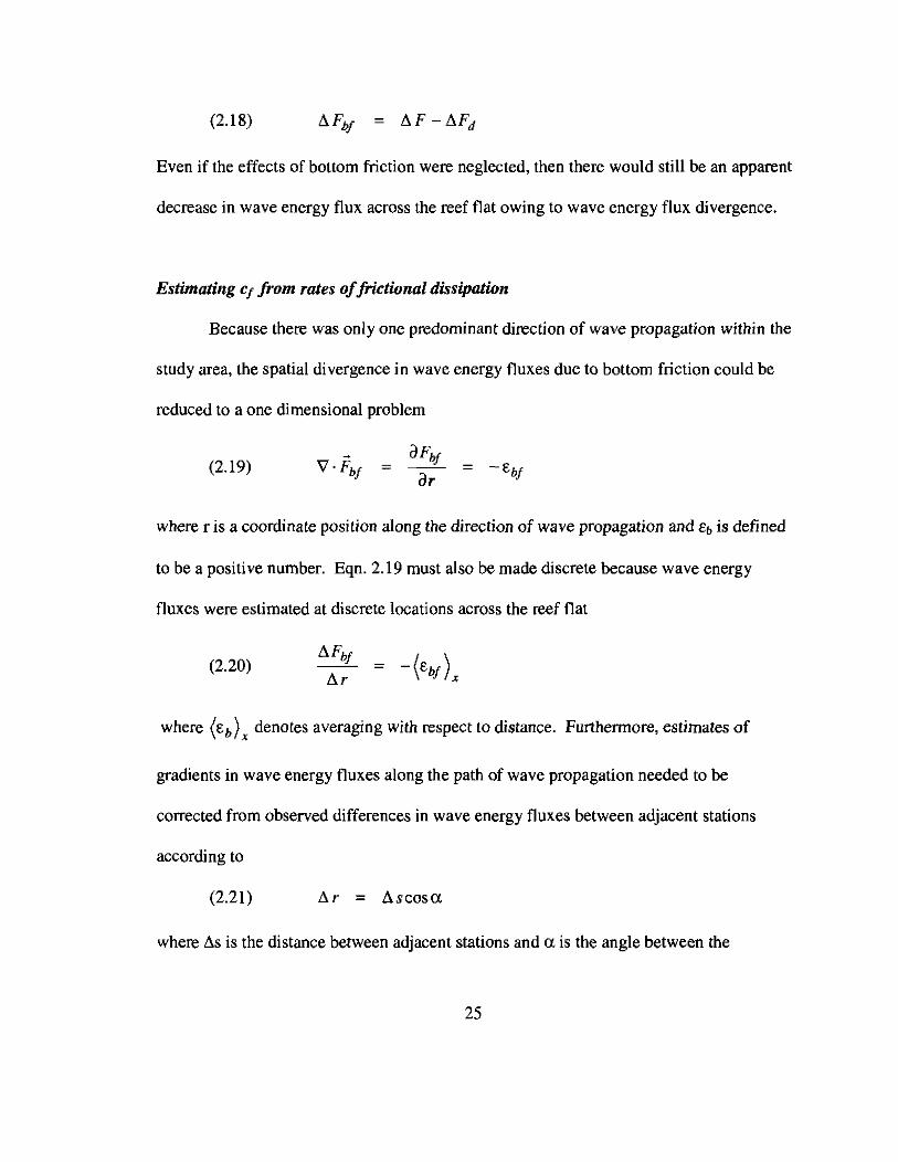
Estimating Cf from frictional dissipation 25

Results 28

Wave heights 28

Wave-driven velocities 34

Cross-reef currents 37

Wave energy flux divergence 37

Estimation of Cf 40

Estimation of k based on Cf .42

vii

Estimates of nutrient mass transfer coefficients ..45

Discussion .46

Comparison of results with other reefs .46

Past estimates of S .47

Variation in S driven by wave transformation 48

Chapter III: Nutrient mass transfer rates derived from the dissolution of plaster

molds 51

Introduction 51

Chapter goals 51

Background: The utility of dissolving plaster surfaces 51

Methods 52

Plaster mold design 53

Mass transfer of Ca2+ 57

Field experiments 61

Flume experiments 66

Estimates of Ca2+ mass transfer coefficients 68

Results 68

Physical parameters 68

Mass transfer rates 75

Flume vs. Field experiments 79

Discussion 79

Importance of varying roughness scales under high Sc 79

Independence of individual element dissolution rates 83

Flume vs. Field experiments 84

Estimates of S for a Kaneohe Bay Barrier Reef flat community 87

Chapter IV: Discussion 89

Comparison different estimates of S 89

Present estimates of S 89

Past estimates of S 91

S for other reef communities 95

Nutrient uptake and net primary production 96

VllJ

Maximum phosphorus and nitrogen fluxes 96

Estimates of net and gross primary production 97

Spatial zonation in reef metabolism 101

Fore reef 102

Reef flat. 105

Comparison with past observations 109

Temporal variation in nutrient uptake rates 110

Variations in the near shore wave field 110

Variability in nutrient concentrations 114

The importance of different time-scales 115

Chapter V: Conclusions 118

References , " 119

ix

List of Tables

Table Page

2.1 Rms-wave heights on the Kaneohe Bay Banier Reef flat.. 29

2.2 Near-bottom flow speeds on the Kaneohe Bay Banier Reef flat.. .37

2.3 Estimates of nutrient mass transfer coefficients .46

2.4 Correlation between flow speeds and tides 50

3.1 Results from field and flume plaster dissolution experiments 73

x

List of Figures

Figure Page

2.1 Results from prior mass transfer experiments .15

2.2 Map of Kaneohe Bay, Oahu, Hawaii 17

2.3 Aerial image of study site: Kaneohe Bay Barrier Reef flat... 19

2.4 Color-stretched image of study site showing wave fronts 20

2.5 Spectra of wave heights across the reef flat on 10 Aug 30

2.6 Spectra of wave heights across the reef flat on 16 Aug 31

2.7 Spectra of wave heights across the reef flat on 4 Sep 32

2.8 Rms-wave heights versus tide 33

2.9 Spectra of Uh from current meters and pressure sensors versus frequency 35

2.10 Spectral densities of Uh from current meters versus from pressure sensors 36

2.11 Mean currents across the reef flat... 38

2.12 Principal direction of wave propagation 39

2.13 Uh3 from current meter versus pressure sensor 41

2.14 Regression yielding estimate of cf 43

3.1 Schematic of mold designs 54

3.2 Ratio of wet to dry plaster densities 57

3.3 Map of plaster deployment sites in Kaneohe Bay 63

3.4 Experimental setup of flume experiments 67

3.5 Plaster mold with holes before and after deployment.. 69

3.6 Early molds before and after deployment.. 70

3.7 Grooved plaster elements before and after deployment... 71

3.8 Sample spectra of near-bottom flow speeds from the field experiments 74

3.9 Dissolution of Ca2+ versus surface area and flow speed 76

3.10 Ca2+ mass transfer coefficients versus a and flow speed from fieldexperiments 77

3.11 Ca2+ mass transfer coefficients versus a and flow speed from flumeexperiments 78

3.12 SUa versus flow speed for both field and flume experiments 80

xi

3.13 St versus flow speed from prior flume experiments 81

4.1 Phosphate concentration versus distance across the reef flat.. 92

4.2 Concentrations of DIP and DIN in waters off Hawaii versus time 98

4.3 Mean directional wave spectrum off windward Oahu, Hawaii .103

4.4 SWAN simulation of wave heights across the fore reef of the Kaneohe BayBarrier Reef 104

4.5 Simulation of near-bottom flow speeds and maximum phosphate uptake ratesacross the fore reef of the Kaneohe Bay Barrier Reef.. 106

4.6 Daily significant heights of trade wind-generated waves and northern swell offwindward Oahu, Hawaii versus time l11

4.7 Variation in daily significant heights of trade wind-generated waves off windwardOahu, Hawaii at different time scales .l16

Xli

List of Symbols

Symbol Description Units

NPP net primary production mmol C m-2 day-l

OPP gross primary production mmol C m-2 dai l

RA autotrophic respiration mmol C m-2 dai'

J molar flux of species mmol m-2 day-l

Jrnax maximum molar flux mmol m-2 day-l

S mass transfer coefficient mdai l

St Stanton number

U ambient flow speed -Ims

Ci,b concentration of species i in the ambient fluid mol m-3

Ci,s concentration of species i at the solid surface mol m-3

Cf friction coefficient

Rek Reynolds roughness number

Sc Schmidt number

'tb benthic shear stress Nm-2

u* shear velocity -Ims

k roughness height m

kinematic viscosity 2 -IV m s

p density of sea water kgm-3

Di diffusivity of species i m2 S-I

Dh hydraulic radius m

Ac flow cross-sectional area m2

P wetted perimeter m

[' empirical mass transfer constant

H wave height m

Hsig significant wave height m

HITlls fills-wave height m

Hmax maximum allowable wave height m

xiii

F wave energy flux J m-1 S-l

fz cnoidaJ wave energy flux constant

gravitational acceleration -2g ms

h water depth m

T wave period s

Eb rate of energy dissipation due to bottom friction Wm-2

Uh horizontal flow speed m2 S-l

fe wave friction factor based on energy dissipation

fw wave friction factor based on maximum shear stress

A wave orbital excursion amplitude m

y depth-induced wave breaking parameter

:ECa2+ sum of free Ca2+ and its ion pairs

:ESOl- sum of free sol- and its ion pairs

z± charge of anion/cation

Ksp solubility product for gypsum mol2 m-6

i\Mea mass of calcium loss mol

PA projected area of plaster mold m2

SA total surface area of plaster mold m2

ex ratio of surface area to projected area

Oe thin-film concentration boundary layer thickness 11m

Re Reynolds number

Suet net nutrient uptake coefficient mdaf'

Q' cross-reef volumetric transport rate m3 S-l m-1

DIP dissolved inorganic phosphate

DIN dissolved inorganic nitrogen

xiv

I

INTRODUCTION

Metabolism ofcoral reefcommunities

Coral reefs were first recognized by Darwin (1842) for their high biomass and

ecological diversity relative to the nutrient- and biomass-poor oceanic waters in which

they live. Subsequent investigations of the metabolism of coral reef communities

revealed that areal rates of photosynthetic production and respiration of organic carbon

by reef communities were one to three orders of magnitude higher than surrounding

pelagic communities (Kinsey 1979, 1985; Odum and Odum 1955; Sargent and Austin

1949, 1954; Smith 1973; Smith and Marsh 1973). The uptake of particulate organic

materials imported by coral reef communities from nearby oceanic waters was not

enough to support observed rates of respiration (Glynn 1973; Odum and Odum 1955;

Sargent and Austin 1949, 1954). Therefore, it was concluded that coral reef communities

must maintain their relatively high rates of metabolism through the recycling of

photosynthetically derived organic matter. This idea was further confirmed by many

observations that rates of photosynthetic production and respiration in most reef flat

communities were nearly equal (Kinsey 1985). Only a small fraction « 10%) of the

organic carbon produced and consumed within most coral reef communities is either

imported or exported (Crossland et al. 1991).

Net primary production (NPP) is defined as the total amount of organic carbon

1

produced by a photosynthetic organism (gross primary production, or GPP) minus the

amount of organic carbon that it consumes through aerobic respiration to meet its basic

metabolic requirements (RA).

(1.1) NPP = GPP - RA

Net primary production is typically interpreted as the amount of organic carbon used to

produce new, living tissue in photosynthetic organisms. This production is important for

providing a source of food to heterotrophic organisms within coral reef communities. It

is perhaps the most important pathway by which mass and energy enter coral reef food

webs. While photosynthesis provides both energy and organic carbon, the production of

new tissue by reef corals and plants requires the uptake and assimilation of nitrogen and

phosphorus. Mass balance states that, to produce new tissue, photosynthetic organisms

must assimilate nutrients and fix organic carbon in a ratio equivalent to the molar ratio of

these elements in their tissues. This ratio is best known for marine phytoplankton. Net

primary production by marine phytoplankton can be described by the following

biogeochemical reaction

(1.2) 106C02 +16N03 + HPol- +18H+ + 122H20 =>

(CHzO)106(NH3)16H3P04 + 13802

where the molar ratio of carbon:nitrogen:phosphorus (C:N:P) in the tissues of marine

phytoplankton is given as 106:16:1 (Redfield et al. 1963).

Pilson and Betzer (1973) estimated rates of nutrient uptake (i.e., dissolved

phosphate) by coral reef communities. They found significant uptake of phosphate along

2

a transect dominated by algae while they found no significant uptake of phosphate along

a transect over a mixed community of coral and algae. For both transects, the net uptake

of phosphate by the algal-dominated community did not scale with observed rates of net

organic carbon production according to the C:P ratio determined for marine

phytoplankton of 106:1 (Eqn. 1.2). Therefore, these authors hypothesized that

phosphorus was being tightly recycled within reef communities in order to support the

observed high rates of photosynthetic production and respiration. Alternatively,

however, they recognized the possibility that the C:P ratios for reef autotrophs could be

much higher than that of plankton and could explain differences in observed and

expected rates of net dissolved phosphate fluxes. However, in a paper summarizing the

collective research done at Enewetak, Johannes et al. (1972) championed the explanation

of tight nutrient recycling.

Subsequent studies of nutrient fluxes to and from coral reef communities

indicated that nutrient fluxes were difficult to detect and, when detected, showed no

consistent pattern (Crossland and Barnes 1983; Crossland et al. 1984; Johannes et al.

1983; Webb et al. 1975). Thus, a clear and coherent paradigm for the nutrient

metabolism of coral reefs was never synthesized. Part of the reason was that past studies

relied on flow respirometry as their method of investigation. In this method, net fluxes of

materials into and out of the reef were estimated from changes in the chemical

composition of water parcels moving across the reef. Flow respirometry was successful

in providing estimates of photosynthetic production, respiration, and calcification rates

for coral reef communities (Kinsey 1979, 1985; Odum and Odum 1955; Sargent and

3

Austin 1949, 1954; Smith 1973; Smith and Marsh 1973). These metabolic processes

provided substantial changes in the composition of waters passing across the reef relative

to the analytical methods used to detect them. Estimates of net nutrient fluxes to reef

communities based on changes in nutrient concentrations approached the analytical limits

of dissolved nutrient detection (Crossland and Barnes 1983; Johannes et al. 1983; Pilson

and Betzer 1973; Webb et al. 1975). Atkinson et al. (Atkinson 1981b, 1987a; Atkinson

and Smith 1987) argued that changes in dissolved nutrient concentrations across reef flat

communities were difficult to detect because the rate at which reef autotrophs can take up

dissolved nutrients is most often too slow to substantially alter the nutrient content in the

sea water passing over them, not because nutrients were being tightly recycled.

Mass transfer limitaiion

By the end of the 1980s, it was clear that most coral reef communities lived in

waters characterized by low concentrations of dissolved nutrients (typically < 0.5 ~)

and that nutrient fluxes to reef communities were very small in comparison with rates of

photosynthetic production and respiration. Yet photosynthetic reef organisms maintained

very high biochemical affinities for dissolved nutrients (Atkinson 1987b; Muscatine and

D'Elia 1978). Consequently, it was possible that rates of nutrient uptake by reef

communities approached some kind of physical rather than biochemical limit. These

ideas led Bilger and Atkinson (1992) to hypothesize that the rate at which reef

communities could take up inorganic nutrients was limited by the rate at which nutrients

could be physically transported across a concentration boundary layer covering the

4

surfaces of reef autotrophs. Nutrient uptake under these conditions is defined as being

mass transfer limited. This theory stated that rates of nutrient uptake by coral reef

communities were controlled by the ambient flow speeds, the frictional roughness of the

community and the diffusivity of the nutrients in question. Interestingly enough, Munk

and Sargent (1954) had proposed a similar idea forty years earlier. They stated that the

scrubbing action of wave-induced flow could reduce the thickness of boundary layers at

the surfaces of the reef in order to promote the exchange of metabolites. Unfortunately,

this concept was ignored at the time it was proposed. Early studies on the nutrient uptake

kinetics of corals attempted to describe them in terms of a classical Michaelis-Menten

model, the convention for describing the nutrient uptake kinetics of phytoplankton

(D'Elia 1977; Muscatine and D'Elia 1978). However, Muscatine and D'Elia (1978)

indicated that a diffusion-based physical transport mechanism (i.e., mass transfer) was

necessary to describe the observed kinetics. Mass transfer limitation of nutrient uptake

has been demonstrated in both small-scale (-1.5 m2) and large-scale (-850 m2

)

experimental reef communities (Atkinson and Bilger 1992; Atkinson et aJ. 1994;

Atkinson et aJ. 2001; Bilger and Atkinson 1995; Lamed and Atkinson 1997; Thomas and

Atkinson 1997).

Nutrient uptake and net primary production

Atkinson (l981a, 1981b) demonstrated that rates of net phosphate uptake by reef

flat communities of the Kaneohe Bay Barrier Reef and Enewetak Atoll could be equated

with rates of net community production by the C:P ratio of the photosynthetic organisms

5

residing within their respective communities. Net community production (NCP) is

defined as the difference between gross primary production and the rate of respiration by

the entire community and is interpreted to be the amount of organic carbon imported or

exported by the community. Consequently, the slow rates of net phosphate uptake

observed in coral reef communities could support their net metabolic needs because the

C:P ratios of benthic autotrophs were much higher than previously thought (Atkinson and

Smith 1983; Pilson and Betzer 1973). Atkinson could not make any estimates of the

amount of gross phosphate uptake necessary to support net primary production because

all estimates of nutrient fluxes based on flow respirometry, by definition, include the

effects of both uptake and excretion. Maximal rates of nutrient uptake by coral reef

communities are nearly impossible to measure directly, even with the introduction of a

tracer (Atkinson and Smith 1987). Therefore, rates of total or gross nutrient uptake by

coral reef communities remain completely unknown.

Little is known about the interaction between net primary production and nutrient

uptake in coral reef communities. Although both the fixation of inorganic carbon and

nutrients are required for the growth of autotrophic tissue, the former process is largely

governed by the absorption and conversion of light energy while the latter is controlled

by the physical interaction of the reef community with their flow environment. Questions

of whether differences in the scales of nutrient uptake rates and net primary production

are responsible for the high C:N and C:P ratios in benthic reef autotrophs, or whether one

metabolic pathway limits the production of autotrophic tissue versus the other, remain

unanswered. Furthermore, if rates of new tissue production by benthic reef autotrophs

6

are limited by rates of nutrient mass transfer, then this process will act as an important

regulator on the quantity and quality of organic matter produced by photosynthetic

organisms. Therefore, if we are to understand anything about net primary production in

coral reef ecosystems, as well as the movement of mass and energy through coral reef

food webs, we must know the rates at which coral reef communities can take up and

assimilate nutrients from the water column. Such information will not only provide

general ecological insight into how coral reef ecosystems function, but will also be of

practical use in the maintenance of coral reefs as recreational, subsistence, and

commercial fisheries.

Goals ofthis dissertation

All prior studies on the mass transfer characteristics of nutrient uptake by reef

communities have been limited to artificially assembled communities within the confines

of an experimental re-circulating flume or mesocosm. Little is known about the nutrient

mass transfer characteristics for natural reef communities under in situ flow conditions.

This is because the frictional roughness of these communities and the flow environments

to which they are exposed have not been well known to coral reef biogeochemists.

Furthermore, prior experiments have told us nothing about whether rates of mass transfer

are different under conditions of oscillatory versus steady flow. Early attempts at

predicting nutrient mass transfer characteristics for natural reef communities have been

made with little attention to the above considerations (Atkinson 1992; Bilger and

Atkinson 1992).

7

The primary goal of this dissertation is to estimate nutrient mass transfer

characteristics for a natural reef community under in situ conditions of wave-dominated

flow. To accomplish this goal, first the frictional roughness of the reef flat community

under wave-driven flow was determined from the attenuation of surface gravity waves

across the community. Second, the flow conditions across the community were directly

measured as well as estimated using a modified linear wave theory. This friction and

flow data were used to estimate dissolved nutrient mass transfer coefficients from mass

transfer correlations tested on experimental coral reef communities. Next, the dissolution

of plaster molds were used to evaluate the differences in mass transfer rates for similar

molds under varying flow conditions as well as to provide a check for estimates of

nutrient mass transfer coefficients based on the application of a mass transfer correlation.

The second goal of this dissertation will be to evaluate the importance of

roughness scale and available surface area on rates of mass transfer under both natural,

oscillatory and experimental, steady flows.

The final goal of this dissertation will be to compare maximum rates of nutrient

uptake allowed by mass transfer for a Kaneohe Bay Barrier Reef flat community with

observed rates of net phosphate uptake and gross photosynthetic production from the

same area. This will allow an assessment of whether rates of nutrient uptake within this

community are operating near the limits of mass transfer and whether net primary

production within this community is largely controlled by nutrient uptake.

8

II

ESTIMATES OF NUTRIENT MASS TRANSFER RATES

FROM LARGE-SCALE WAVE TRANSFORMATIONS

Introduction

Approach

The objective of this chapter is to estimate nutrient mass transfer coefficients for a

community on the Kaneohe Bay Banier Reef. The first part of this chapter will review

and simplify existing mass transfer correlations that have been applied to experimental

coral reef communities in previous studies. These correlations relate the mass transfer

characteristics of a given community to its frictional roughness and the flow speeds to

which it is exposed. The frictional roughness of a reef community is represented by the

friction coefficient, Cf, which relates the amount of frictional force per unit area that is

generated by the community under a given ambient flow speed. In this study, the value

of the friction coefficient will be estimated from the attenuation of waves across the reef

flat as measured by four pressure sensors deployed in a linear array -100 m apart, and

one current meter deployed along side the pressure sensor closest to the fore reef. The

resulting data on wave-driven flow speeds will be used to obtain an estimate of Cf for the

reef flat community, and to ultimately generate estimates of nutrient mass transfer

9

coefficients across the community. Finally, spatial and temporal variation in these

estimates will be discussed.

Coral reefmass transfer relationships

Mass transfer theory states that the molar flux of a given species, h to a surface

under a given set of flow conditions can be related to the concentration of that species at

the surface, Chs, and in the bulk fluid Cj,b, by the molar mass transfer coefficient, Sj

(2.1) = S.(C· b - C. )I I, ItS

If Cj,b » Chw, then the molar flux approaches a maximum mass-transfer rate of

The mass transfer parameterization used by Atkinson et al. (Baird and Atkinson

1997; Bilger and Atkinson 1992, 1995; Thomas and Atkinson 1997) was based on the

dimensionless Stanton number, Stj, which relates Sj to the ambienty flow speed, U

(2.3)

Dade (1993) generalized an expression for St based upon the heat transfer correlations of

Dipprey and Sabersky (1963) as well as the mass transfer correlations of Dawson and

Trass (1972)

(2.4) =1 + ~(ef /2) (yRe!: Set - 8.48)

where Cf is the friction coefficient which relates the magnitude of benthic shear stress, 'tb,

toU

10

where Rek is the Reynolds roughness number defined as

(2.6)

where k is the roughness height, v is the kinematic viscosity of the fluid, and u* is the

friction velocity defined as

(2.7) u* '" ~~

SCi is the Schmidt number of specific dissolved nutrient i and is defined as the ratio of the

kinematic viscosity of the fluid to the molecular diffusivity of that nutrient (Di) in the

fluid (SCi'" VlDi). The empirical constants a, b, and y in Eqn. 2.4 are taken from the heat

transfer correlation of Dipprey and Sabersky (1963) and the mass transfer correlation of

Dawson and Trass (1972).

Heat transfer correlations are based on the Prandtl number, Pr, which is defined as

the ratio of the kinematic viscosity of a fluid to the diffusivity of thermal energy (a) in

that fluid (Pr '" via). This non-dimensional number is analogous to Sc used in mass

transfer correlations. The Chilton-Colburn analogy states that for fluids with high Pr and

Sc, the heat and mass transfer correlations are analogous. Dade (1993) considered the

problem of nutrient mass transfer from rippled sediment beds, a problem analogous to

nutrient mass transfer to coral reef communities. Therefore, Dade (1993) could use the

heat transfer correlation of Dipprey and Sabersky (1963) to describe mass transfer by

11

analogy through substitution of its dependency on Pr with an equivalent dependency on

Sc. Sc for dissolved inorganic nutrients in waters around coral reefs are typically> 500.

The heat transfer correlation of Dipprey and Sabersky extends to higher Rek than does the

mass transfer correlation of Dawson and Trass correlation (2400 vs. 120). However, the

correlation of Dawson and Trass extends to higher values of Sc than the Dipprey and

Sabersky correlation extends for Pr (4600 vs. 6).

Thomas and Atkinson (1997) and Baird and Atkinson (1997) used Eqn. 2.4 with

the parameter values from Dipprey and Sabersky (1963) to estimate mass transfer

coefficients for experimental communities of coral and coral rubble. In these

experiments, U was directly measured, Cf was estimated from head-loss across the

experimental communities while v and p were calculated from the known temperature

and salinity of the water. Baird and Atkinson (1997) recognized the difficulty of

measuring k for irregularly rough communities, such as those found on coral reefs, and

suggested that k be estimated from the frictional characteristics of the community (as

represented by Cf) according to an explicit expression put forth by Haaland (1983) and

used by Bilger and Atkinson (1992)

(2.8) [ ( )1.11]1 6.9 k-- = -3.6 log -+

~ Re 3.7D.

where Dh is the hydraulic diameter of the experimental flume, Re is the Reynolds

number, and the Darcy-Weisbach friction factor, f, has been replaced by Cf (f == 4cr). Dh

12

is calculated from the ratio of the cross-sectional flow area, Ac, to the wetted perimeter of

the flow channel, P, by

(2.9)4A,

P

Eqn. 2.8 is actually a synthesis of expressions relating Cf to k for both smooth and

rough surfaces (Haaland 1983). If we consider only turbulent flow over rough surfaces,

which should be appropriate for most reef communities, then the simpler von Karman

expression for turbulent flow over rough surfaces from which Eqn. 2.8 is formulated can

be used:

(2.10)1

F;= -410g( k )

3.7 Dh

The data of Thomas and Atkinson (1997) and Baird and Atkinson (1997) can be

directly compared by applying Eqns. 2.4-2.7 and using values for k estimated from Cf

according to Eqn. 2.10, as well as a value of a =0.2 taken from the more relevant high

Rek data of Dipprey and Sabersky (1963) and a value of b = 0.58 taken from the more

relevant high Sc data of Dawson and Trass (1972). Assuming that the roughness heights

of most reefs are typically no less than 0.01 m, bulk flow velocities are no less than 0.02

m S·I, and values of Cf are no less than one fifth the minimum published value (= 0.005),

then Rek for most reef environments should be no less than _102. This means that only

the term involving Rek and Sc is the most important term in the denominator of Eqn. 2.4.

The value of 8.48 in the denominator of Eqn. 2.4 contributes less than 2% to the

calculation of St; thus, Eqns. 3 and 4 can be combined and simplified into an equation for

13

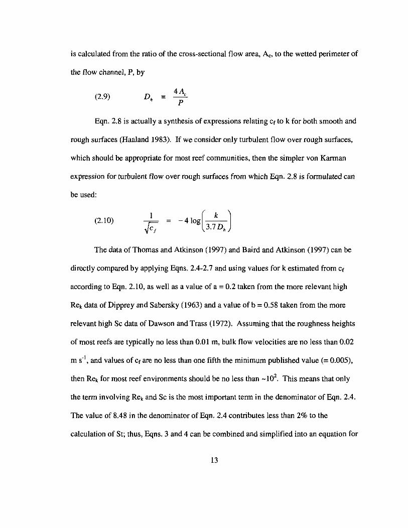
predicting S; based on the following approximation

(2.11) ~ r~uRekSci

where r is an empirical constant which depends upon the values chosen for a and b.

This approximation more clearly shows how nutrient mass transfer to coral reef

communities directly depends on the non-dimensional quantities Ct, Sc, and Rek than the

expression given in Egn. 2.4. Mass transfer coefficients measured from the uptake of

ammonium by experimental reef communities (Thomas and Atkinson 1997) are in very

good agreement with the dissolution of gypsum-coated corals (Baird and Atkinson 1997)

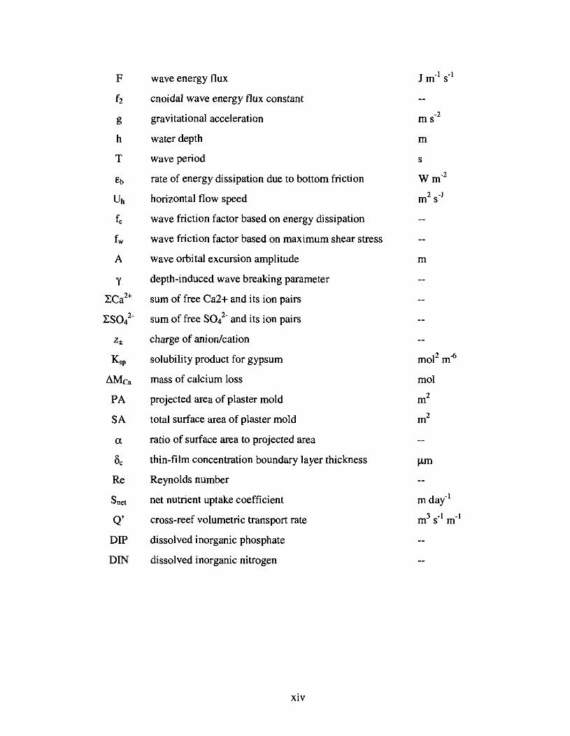
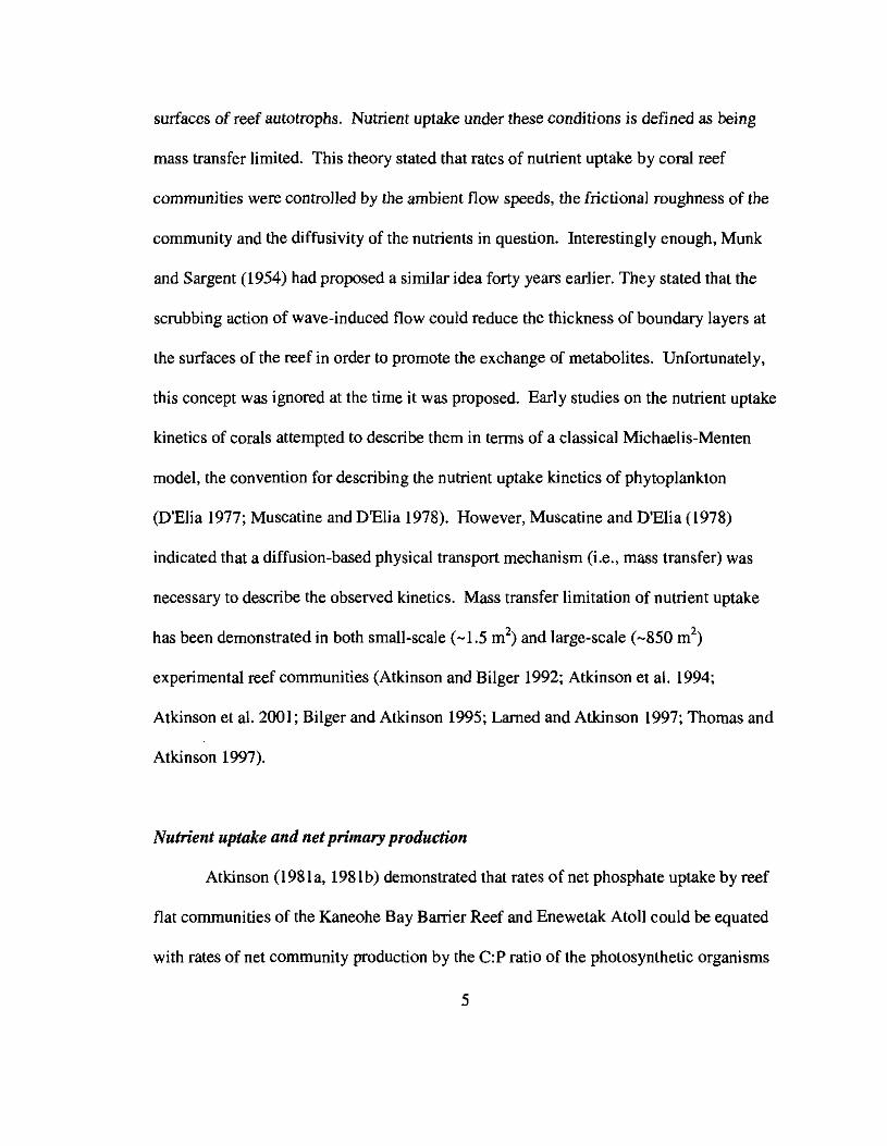
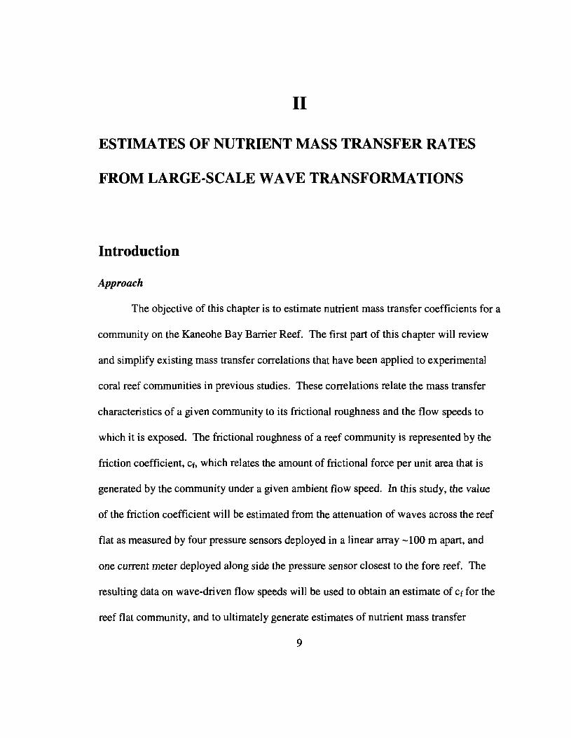
as described by the functional relationship given in Eqn. 2.11 (C = 0.95; Fig. 2.1). These

results not only demonstrate that nutrient uptake by experimental reef communities

occurs at the limits of mass transfer, but can be predicted from existing mass transfer

relationships.

If Egn. 2.11 is dimensionalized, then the following relationship results:

(2.12) Si

D j for a specific dissolved nutrient and v can be calculated based upon the salinity and

temperature of sea water (Li and Gregory 1974). Therefore, Eqn. 2.12 can be used to

estimate the nutrient mass transfer coefficient (S;) once Ct, U, and k are known.

From Eqn. 2.12 it also follows that S; is proportional to the benthic shear stress

raised to the 0.4 power

14

(2.13) S ~o.•i OC "b

This proportionality was corroborated by Hearn et al. (2001) who derived a similar

expression based on a separate mass transfer relationship proposed by Batchelor (1967).

1.6

1.4

1.2

.-..'10 1.0 V'..... (>x~ 0,(j)

0.8E-II> + ..

'"III 0.6 V'V'E(J) ..

V'

0.4 +V'

0.2

(>

V' gypsumo HR rubble.. LR rubble(> P. compressa+ P. damicomis

oL-__L--_-J'---_-----l__---'__---'__---'__-.J

o 0.5 1.0 1.5 2.0 2.5 3.0 3.5

UJcf /2 1-40.2 0.58 (m S- x10 )

Rek SCi

Figure 2.1 Measured mass transfer coefficients for experimental reefcommunities based on ammonium fluxes (Thomas and Atkinson, 1997) andcalcium fluxes (Baird and Atkinson, 1997) versus the quotient term in Eqn. 2.11.The model II regression shown is Y = 0.47X - 4e-6 ((! = 0.95, n = 29).

15

Methods

The purpose of this section is to show how Cr, U, and k across a Kaneohe Bay

Barrier Reef flat community can be derived from measuring the height of waves

propagating over the community. These values will be used to estimate the nutrient mass

transfer coefficients for the community according to Eqn. 2.12.

Site description

Kaneohe Bay is located on the northeast, or windward, side of the island of Oahu,

Hawaii. The Kaneohe Bay Barrier Reef is roughly 2 km wide and 10 km long, running

NW to SE along the entrance of Kaneohe Bay (Fig. 2.2). The only emergent structure on

the Kaneohe Bay Barrier Reef is Kapapa Island. Most of the rest of the Kaneohe Bay

Barrier Reef, including the reef flat and reef crest, remains submerged during all phases

of the tide. The back-middle of the reef flat, however, becomes exposed only during very

low tides. The depth of the reef flat ranges from < 1 m to -3 m with a general trend in

shoaling going from the reef crest to the back reef and from the Sampan and ship

channels bounding each side of the reef to the middle of the reef flat. Despite the lack of

emergent features, the presence of channels, and deeper portions of the reef flat, the

Kaneohe Bay Barrier Reef is still very effective at dissipating the flux of wave energy

incident to Kaneohe Bay. There are two primary sources of wave energy impinging on

the Kaneohe Bay Barrier Reef: 1) wind waves 6-10 s in period generated by trade winds

which blowout of the east to northeast all year round, but are most consistent during the

16

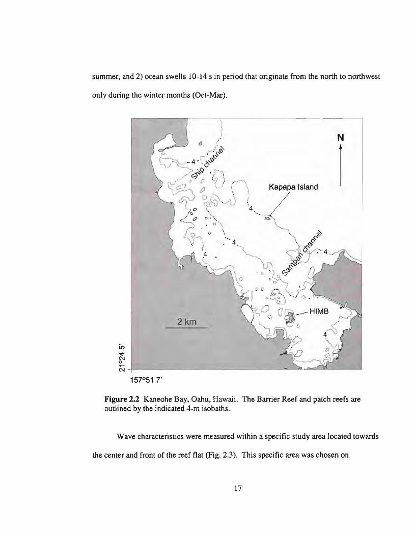
summer, and 2) ocean swells 10-14 s in period that originate from the north to northwest

only during the winter months (Oct-Mar).

N

Kapapa Island

2km

Lo

~~

N-t-"---------------~-----"'.........,~---'-'-------"

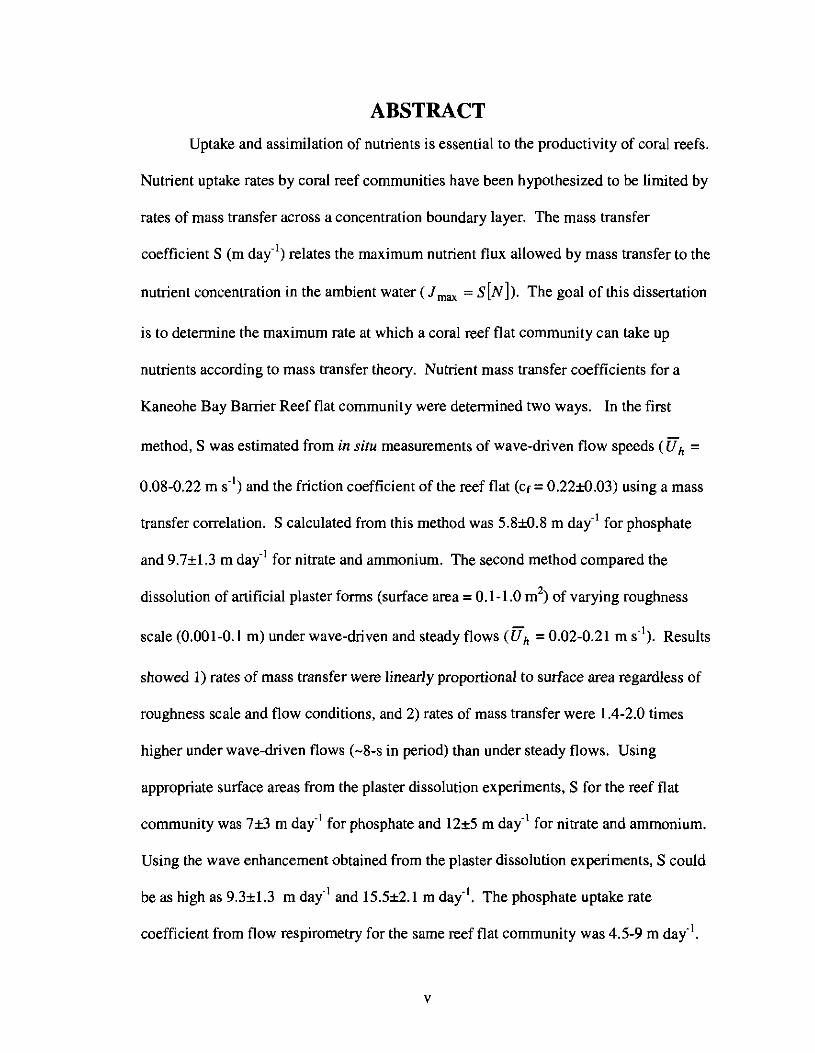
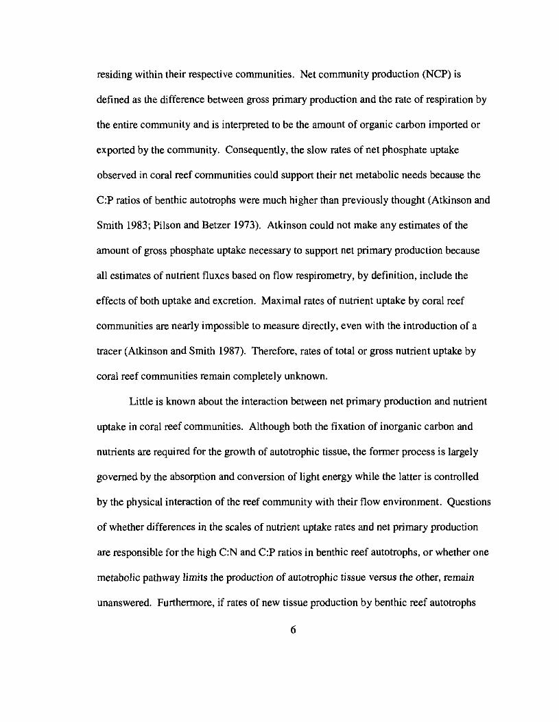
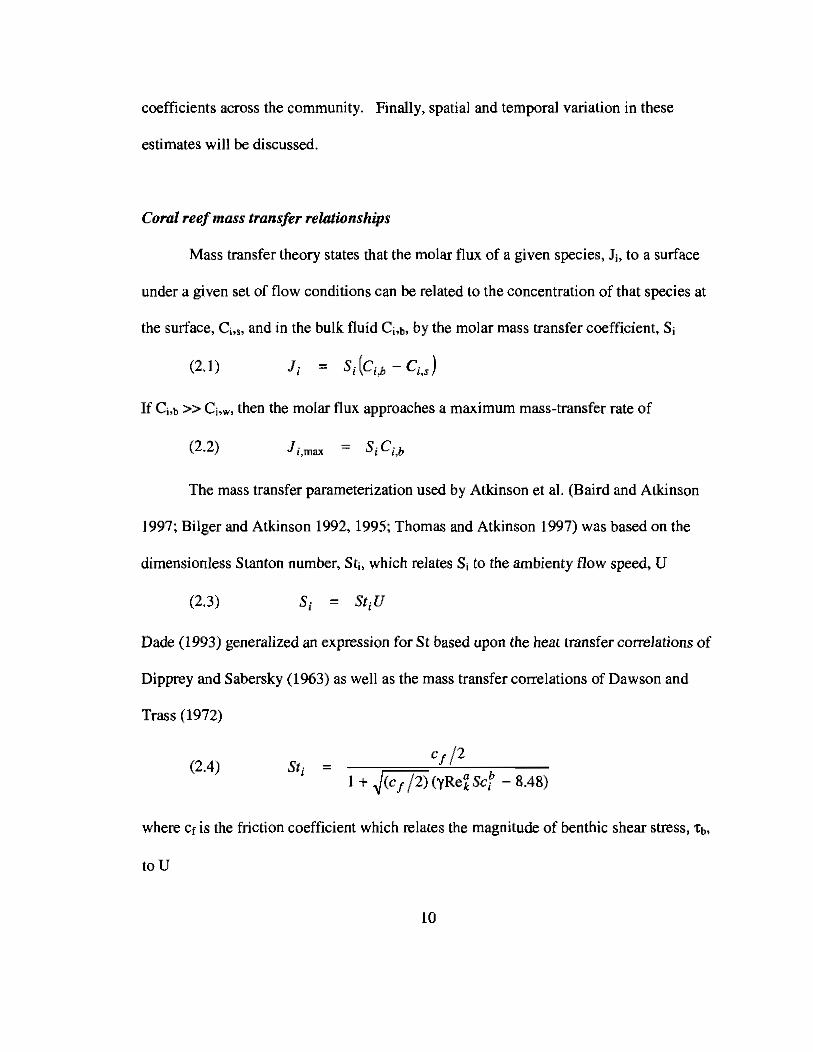
Figure 2.2 Kaneohe Bay, Oahu, Hawaii. The Barrier Reef and patch reefs areoutlined by the indicated 4-m isobaths.

Wave characteristics were measured within a specific study area located towards

the center and front of the reef flat (Fig. 2.3). This specific area was chosen on

17

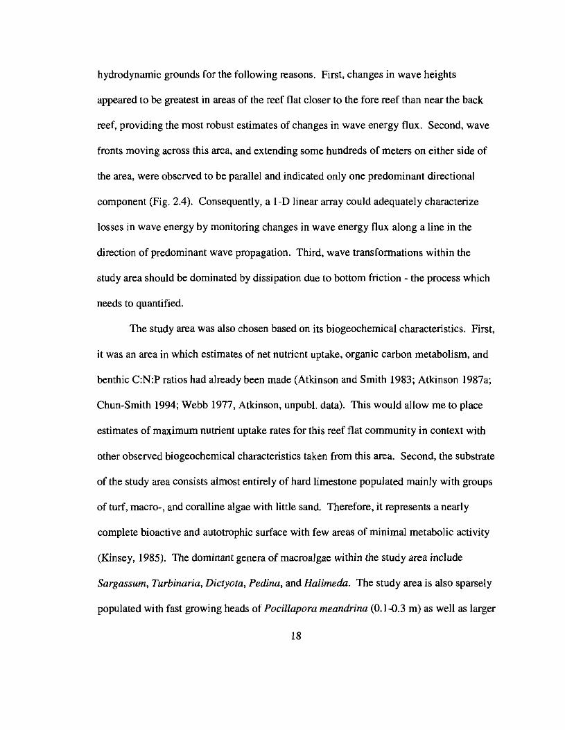
hydrodynamic grounds for the following reasons. First, changes in wave heights

appeared to be greatest in areas of the reef flat closer to the fore reef than near the back

reef, providing the most robust estimates of changes in wave energy flux. Second, wave

fronts moving across this area, and extending some hundreds of meters on either side of

the area, were observed to be parallel and indicated only one predominant directional

component (Fig. 2.4). Consequently, a 1-0 linear array could adequately characterize

losses in wave energy by monitoring changes in wave energy flux along a line in the

direction of predominant wave propagation. Third, wave transformations within the

study area should be dominated by dissipation due to bottom friction - the process which

needs to quantified.

The study area was also chosen based on its biogeochemical characteristics. First,

it was an area in which estimates of net nutrient uptake, organic carbon metabolism, and

benthic C:N:P ratios had already been made (Atkinson and Smith 1983; Atkinson 1987a;

Chun-Smith 1994; Webb 1977, Atkinson, unpub1. data). This would allow me to place

estimates of maximum nutrient uptake rates for this reef flat community in context with

other observed biogeochemical characteristics taken from this area. Second, the substrate

of the study area consists almost entirely of hard limestone populated mainly with groups

of turf, macro-, and coralline algae with little sand. Therefore, it represents a nearly

complete bioactive and autotrophic surface with few areas of minimal metabolic activity

(Kinsey, 1985). The dominant genera of macroalgae within the study area include

Sargassum, Turbinaria, Dictyota, Pedina, and Halimeda. The study area is also sparsely

populated with fast growing heads of Pocillapora meandrina (0.1-0.3 m) as well as larger

18

heads of Porites [obata (0.5-1.5 m); however, corals represent a very small percentage of

bottom type within the study area.

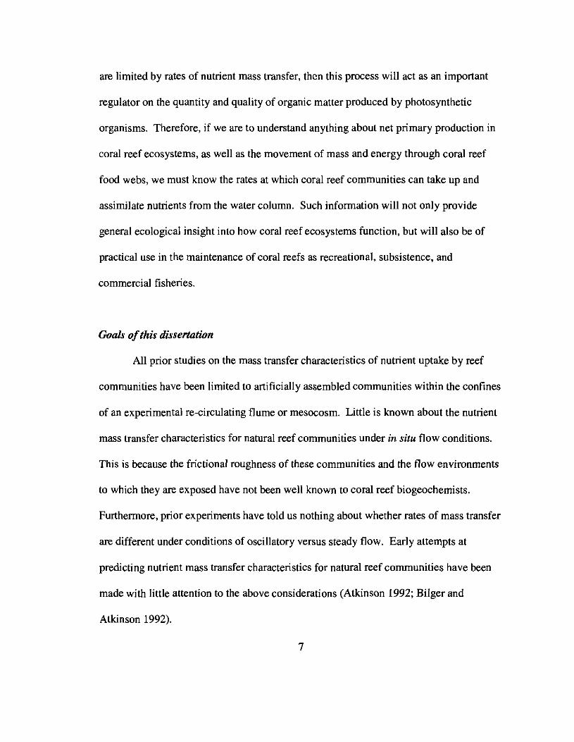
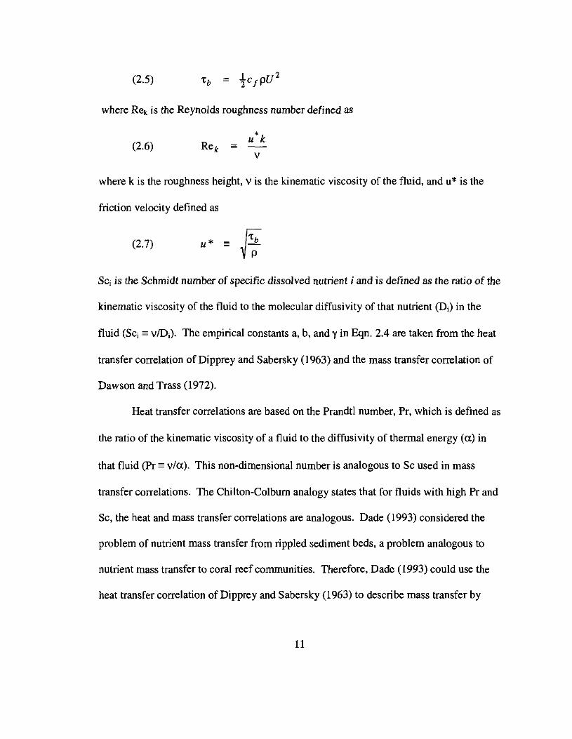
Figure 2.3 Instrument locations on the Kaneohe Bay Barrier Reef flat. Stationswere ordinally numbered according to distance from the fore reef. Diamondsrepresent stations where both a current meter and a pressure sensor weredeployed. Circles mark stations where only a pressure sensor was deployed. Thedark color of the study area indicates nearly 100% coverage of the benthos withalgae and coral. Aerial image taken by AURORA and processed by E. Hochberg.

19

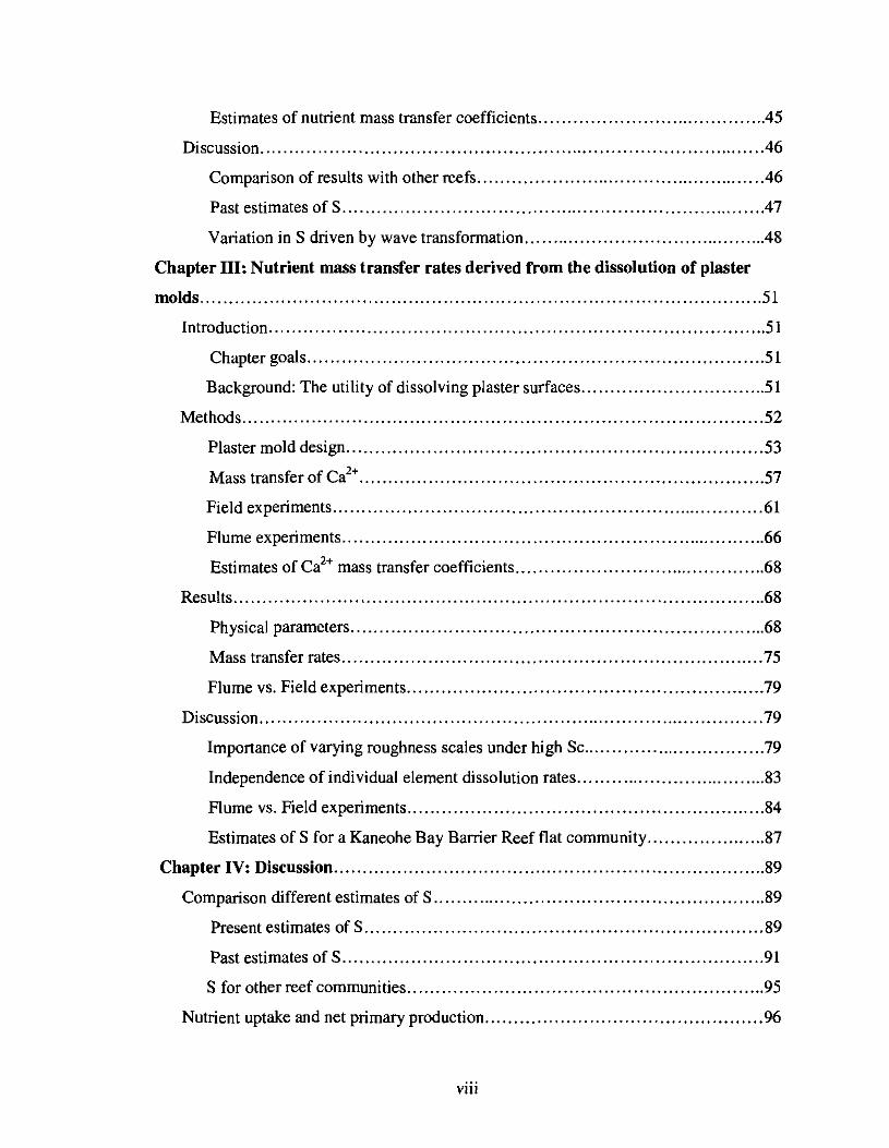
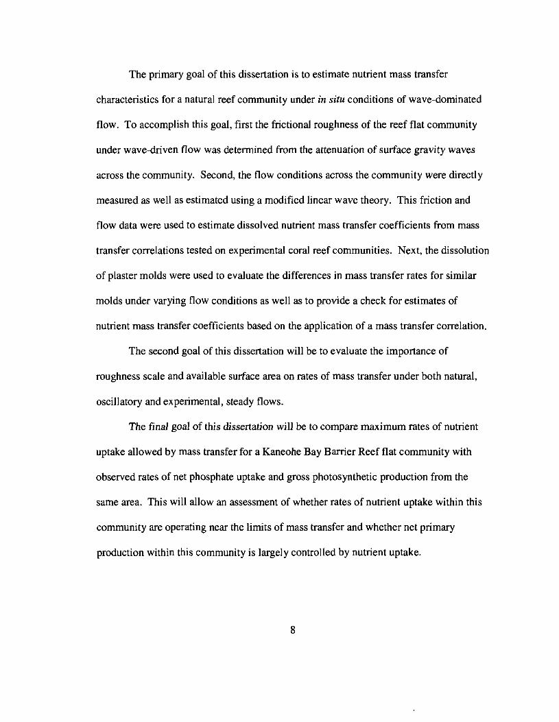
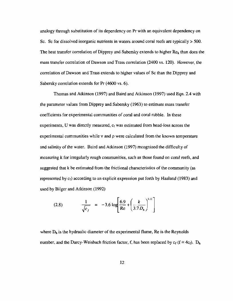
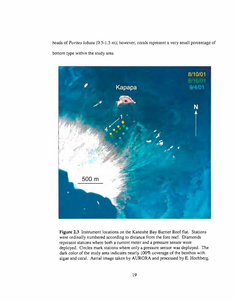
Figure 2.4 Same aerial image as shown in Fig. 2.3, but color-stretched toenhance the appearance of wave fronts. Select wave fronts are highlighted byyellow lines.

Wave height measurements

Wave heights across the reef flat were measured on three different days

corresponding to three different levels of incident wave activity during the summer of

2001 (10 Aug, 16 Aug, and 4 Sep). The dates used throughout this text represent the

days on which the instruments were taken from the water. These measurements were

made during the summer to ensure that the directional spectrum of waves incident to the

20

Kaneohe Bay Barrier Reef would have only one source: the trade winds. On each day

four Seabird SBE-26 pressure sensors (Seabird Electronics, Bellevue, Washington) were

deployed -100 m apart in a linear array following the direction of predominant wave

propagation with the first sensor located -50 m from the back of the surf zone (Fig. 2.3).

The purpose for allowing space between the back of the breaking zone and the first

station of the array was to allow broken waves to fully reform and to prevent the

measurement of wave energy fluxes in an area prone to secondary breaking. In addition,

the landward extent of the breaking zone can migrate in accordance with tidal changes in

the depth of the reef flat. All pressure sensors were deployed on the bottom and

programmed to sample at 2 Hz in fifteen minute-bursts every half hour, yielding 900

samples per burst. Each deployment lasted for approximately one day, yielding 40-43

wave bursts per deployment. The one-sided power spectral densities for wave height

were calculated from the pressure sensor data using linear wave theory (Dean and

Dalrymple, 1991). Each burst was treated as a single record and the resulting spectra

from each burst was band-averaged by 10 fundamental frequencies into bands 1/90 Hz

wide. Rms-wave heights, Hrms, were calculated for each burst from the total spectral

energy during each burst (Horikawa 1988).

Average significant wave heights (Hsig) outside the Kaneohe Bay Barrier Reef

were measured every half hour with a directional wave buoy (Datawell, Netherlands)

deployed"" 5 km off the Mokapu Peninsula, southeast of Kaneohe Bay (21°24.9'N,

157°40.7'W). Hsig is equal to .J2. H nns (Horikawa 1988).

21

Velocity measurements

A MAVS-3 three dimensional current meter (NOBSKA, Mashpee,

Massachusetts) was deployed -1 m away from the pressure sensor closest to the fore reef

on each of the three days (Fig. 2.3). The current meter was zero-calibrated in still water

before each deployment and mounted in a free-standing, weighted tripod with its sensor

positioned 0.5 m off the bottom. Data from the u and v axes (i.e., the two horizontal

axes) of the current meter were used to estimate the predominant direction of wave

propagation by identifying the first principal component axis for each wave burst in u-v

space.

Wave energy fluxes

Waves propagating in shallow water develop a non-linear wave form (Dean and

Dalrymple 1991). For shallow water waves, cnoidal wave theory provides the best

description of wave dynamics and kinematics (Horikawa 1988). Isobe (1985) simplified

the description of finite-amplitude waves in shallow water using first-order cnoidal wave

theory. He gave the following expression for the wave energy flux, F

(2.14) F = f2PgH 2{ih

where p is the density of sea water, g is the gravitational acceleration constant, H is the

wave height, and h is the depth of the water. The value of the constant f2 depends on the

degree to which the wave form is non-linear. The shape of the wave can be fully

described by its associated cnoidal functions, however, Isobe (1985) created a simple

22

look-up table for the value of f2 based upon a wave-shape parameter called the shallow

water Ursell number, Us, which is defined as

(2.15) Us '"gHT 2

h 2

where T is the wave period. Higher values of Us represent increasingly non-linear wave

forms. As Us approaches I, the value of f2 approaches 0.125 and Eqn. 2.15 approaches

the exact expression of F for shallow-water, linear waves. As Us gets larger, the value of

f2 decreases continuously to a value of 0.0822 for Us equal to 200. This reflects the

lower wave-energy density under an increasingly non-linear cnoidal wave form than

would be predicted from linear wave theory (Horikawa 1988). F and Us were calculated

for each burst using the rms-average wave height and peak spectral period. The rms-

wave height was chosen since it represented an average value of the wave energy density

recorded over the length of each burst. The depth of the water, h, was determined by the

mean bottom pressure during each burst.

CorrectWns for wave flux divergence

Increases in the flux of wave energy along the direction of wave propagation can

occur due to the presence of energy sources such as wind stress and from convergence

due to refraction. Decreases in the flux of wave energy along the direction of

propagation can occur due to the presence of energy sinks such as breaking and bottom

dissipation, and also from divergence due to refraction and diffraction. The area studied

here was chosen to be well within the limits of the breaking zone so that wave breaking

23

would not be a factor in changing wave energy fluxes. Substantial changes in wave

height and wave energy density occurred over tens to hundreds of meters. This is much

too small a fetch for the predominant trade winds to add significant amounts of energy to

surface waves propagating across the study area. Therefore, wind inputs were also

neglected.

There was some evidence of the divergence of wave fronts near the back side of

Kapapa Island as well as over a slight!y shallower part of the reef flat adjacent to the

study area. This apparent loss can be estimated by conserving the total flux of energy

along the length of an arc between adjacent wave-ray paths (Dean and Dalrymple 1991).

Thus, the predicted wave energy flux at one point along the wave-ray path can be

estimated from the wave-energy flux at a point upstream by their respective radii of

curvature, Ri

(2.16)

where the subscripts i and i+1 represent adjacent stations. The expected change in wave

energy flux owing to divergence would then be given as

(2.17) = Fi(I-~)Ri+1

Changes in wave-energy fluxes due to bottom friction, IJ.Fb , were then estimated from

the observed differences in wave energy fluxes, IJ.F , by subtracting the effects of wave

divergence according to

24

(2.18)

Even if the effects of bottom friction were neglected, then there would still be an apparent

decrease in wave energy flux across the reef flat owing to wave energy flux divergence.

Estimating cf from rates offrictio1Ull dissipation

Because there was only one predominant direction of wave propagation within the

study area, the spatial divergence in wave energy fluxes due to bottom friction could be

reduced to a one dimensional problem

(2.19)

where r is a coordinate position along the direction of wave propagation and fb is defined

to be a positive number. Eqn. 2.19 must also be made discrete because wave energy

fluxes were estimated at discrete locations across the reef flat

(2.20)

where (fb) x denotes averaging with respect to distance. Furthermore, estimates of

gradients in wave energy fluxes along the path of wave propagation needed to be

corrected from observed differences in wave energy fluxes between adjacent stations

according to

(2.21) !'>.r = !'>.scosa

where !'>.s is the distance between adjacent stations and a is the angle between the

25

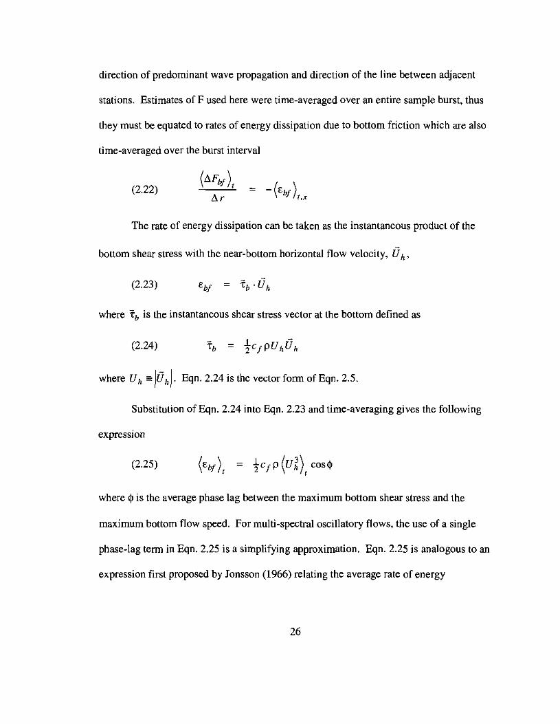
direction of predominant wave propagation and direction of the line between adjacent

stations. Estimates of F used here were time-averaged over an entire sample burst, thus

they must be equated to rates of energy dissipation due to bottom friction which are also

time-averaged over the burst interval

(2.22)

The rate of energy dissipation can be taken as the instantaneous product of the

bottom shear stress with the near-bottom horizontal flow velocity, 6h'

(2.23)

where Tb is the instantaneous shear stress vector at the bottom defined as

(2.24)

where Uh'" 16hi. Eqn. 2.24 is the vectorform of Eqn. 2.5.

Substitution of Eqn. 2.24 into Eqn. 2.23 and time-averaging gives the following

expression

(2.25)

where <p is the average phase lag between the maximum bottom shear stress and the

maximum bottom flow speed. For multi-spectral oscillatory flows, the use of a single

phase-lag term in Eqn. 2.25 is a simplifying approximation. Eqn. 2.25 is analogous to an

expression first proposed by Jonsson (1966) relating the average rate of energy

26

dissipation due to bottom friction to the maximum flow velocity in simple hannonic flow

rUb = Urnsin(wt)]

(2.26)

where Urn is the maximum flow speed. Jonsson (1966) defined fe based on energy

dissipation in order to distinguish it from the friction factor used for estimating maximum

bottom shear stresses (fw) based on the observed and predicted phase lag between bottom

shear stress and velocity under sinusoidal flows (<p). It can easily be shown that if the

phase lag, <p, is neglected, Cf'" fe. For laminar flows, this phase lag is 45°. For turbulent

flow over relatively small roughness elements this phase lag is only'" 25° (Jonsson 1966;

Jonsson 1980). Consequently, for rough, turbulent, sinusoidal flows, fe should be at least

90% the value of Cf. A review of the literature indicates that there should be little

difference between fe and Cf for surfaces with friction coefficients in excess of 0.05

(Nielsen 1992). In the present chapter, I make no discrimination between Cf and fe and,

therefore, choose to use Cf in order to be consistent with prior mass transfer and nutrient

uptake literature.

Averaging Eqn. 2.25 over space and replacing it in Eqn. 2.20 gives us an

expression relating the difference in the time-averaged wave energy flux, the time- and

space-averaged horizontal velocity cubed, and Cf

(2.27)

27

where the subscripts outside the brackets denote an average with respect to time and

space. (u ~) was calculated as the mean of (u ~) from each adjacent pair ofI,X I,X

stations, which is equivalent to assuming that (U~)I varied linearly between stations. By

plotting the left-hand term in Eqn. 2.27 versus (u ~) we can use the model III,x

regression slope to get an average value of Cr for the reef flat community.

Results

S is dependent upon Uh, Cr, and k (Eqn. 2.12). Thus, these parameters needed to

be estimated and/or measured from the characteristics of waves propagating across the

reef flat.

Wave heights

The mean significant heights of waves outside Kaneohe Bay during sampling

were 1.9 m (10 Aug), 1.6 m (16 Aug), and 1.3 m (4 Sep). These values were lower than

the mean daily significant wave height of 2.0 m over the two-year period between Aug

2000 and lun 2002. HIm, decreased 0.15 - 0.25 m across the reef flat from the most

seaward to most landward stations (Table 2.1). Differences in Hnns across the reef flat

between the three days varied according to differences in H'ig outside Kaneohe Bay

(Table 2.1). Mean wave spectral densities appear to be distributed in a broad, single-

peaked band from 0.05 to -0.35 Hz (Fig. 2.5-2.7). The absence of any significant energy

28

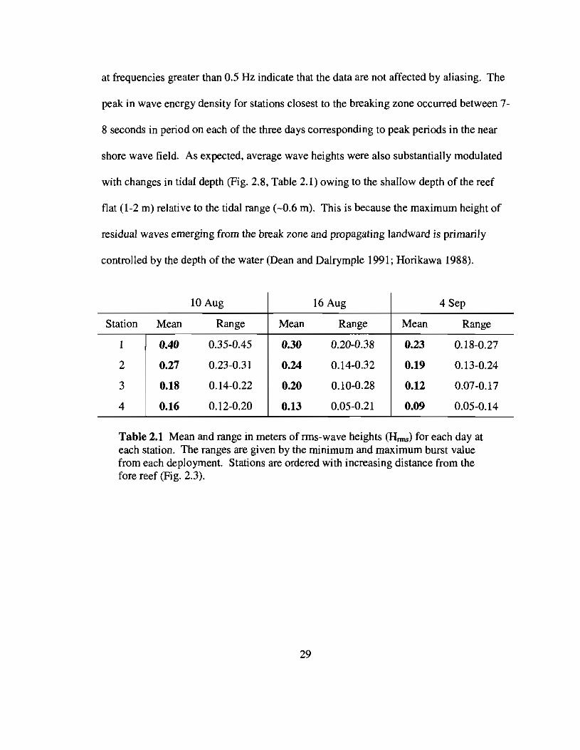
at frequencies greater than 0.5 Hz indicate that the data are not affected by aliasing. The

peak in wave energy density for stations closest to the breaking zone occurred between 7-

8 seconds in period on each of the three days corresponding to peak periods in the near

shore wave field. As expected, average wave heights were also substantially modulated

with changes in tidal depth (Fig. 2.8, Table 2.1) owing to the shallow depth of the reef

flat (1-2 m) relative to the tidal range (-0.6 m). This is because the maximum height of

residual waves emerging from the break zone and propagating landward is primarily

controlled by the depth of the water (Dean and Dalrymple 1991; Horikawa 1988).

10 Aug 16 Aug 4Sep

Station Mean Range Mean Range Mean Range

1 0.40 0.35-0.45 0.30 0.20-0.38 0.23 0.18-0.27

2 0.27 0.23-0.31 0.24 0.14-0.32 0.19 0.13-0.24

3 0.18 0.14-0.22 0.20 0.10-0.28 0.12 0.07-0.17

4 0.16 0.12-0.20 0.13 0.05-0.21 0.09 0.05-0.14

Table 2.1 Mean and range in meters of rrns-wave heights (Hrms) for each day ateach station. The ranges are given by the minimum and maximum burst valuefrom each deployment. Stations are ordered with increasing distance from thefore reef (Fig. 2.3).

29

0.8r------------, 0.8.----------,

0.63

10.5

2

4

0.4

o~_...::::2~ ~

o0.8r-----------,

0.6

0.2

0.6

1

1

0.5

0.4

1\, ': \, ', ': \: \, \

: \.f\ \i \ .,,,\ "

ii " v,.' ,'1 ~" ""

'>/ '-'---::'=:~:::--'0'--------==------'o

0.8.----------,

0.2

0.6

~'(jjcQ)

o~t3Q)c.(j)

0.4 0.4

0.2

O~-o 0.5 1

0.2

Frequency (Hz)

Figure 2.5 Power spectral densities of surface wave height for each of the fourstations on 10 Aug 2001. Mean spectra are given by the thick black line. Thegray regions represent the 95% confidence interval for the mean spectra. Thedashed lines represent one standard deviation for all spectra. Stations are orderedwith increasing distance from the fore reef.

30

0.5 0.5

10.4 ;\ 0.4

: \: '1',

0.3' ,

0.3i \, ,/\: "

~ : \ ' ,~

J v,, 0.2 \ 0.2 : \N " ' ""

, ,I ' ,

,.\ : ''/,N

0.1: '-",

E \, 0.1 \~ .', .. """ ....., ",~ '<~:~'.-:::~: -~'.-..~~::':.:::.:..'00 0 0c: 0 0.5 1 0 0.5(J)

0 0.5 0.5co3....

t5(J) 0.4 0.4a.

(I)

0.3 0.3

0.2 0.2

0.1 0.1

0 0 8:>-0 0.5 1 0 0.5

Frequency (Hz)

2

4

1

1

Figure 2.6 Power spectral densities of surface wave height for each of the fourstations on 16 Aug 2001. Mean spectra are given by the thick black line. Thegray regions represent the 95% confidence interval for the mean spectra. Thedashed lines represent one standard deviation for all spectra. Stations are orderedwith increasing distance from the fore reef.

31

0.25~----~---~ 0.25~---------~

1

2

4

0.20

0.20

0.15

1

3

0.20

0.15

l""""", ,: \, ,, , ,

0.15 i i 0.15 iiI : ,'\I , I'

: \~, ,J \

: \/\ : 1

0.10 !..,' '\ 0.10 ! i,.\ii\.r",\\ i \

1 0.05) ... \'\.::~::::::.::: 0.05 :~:/j\\',,<~>:::~::::...::..~ 0 L- ---""""' ..J 0'i!j 0 0.5 1 0 0.5OJo 0.25 0.25r------------,

-Ue

0.20OJa.

00

0.10 0.10

0.5

0.05 ,.I •• j;;;::"

o ~:.~>1 0

Frequency (Hz)

0.5 1

Figure 2.7 Power spectral densities of surface wave height for each of the fourstations on 4 Sep 2001. Mean spectra are given by the thick black line. The grayregions represent the 95% confidence interval for the mean spectra. The dashedlines represent one standard deviation for all spectra. Stations are ordered withincreasing distance from the fore reef.

32

Figure 2.8 Depth (dashed line) and rms-wave height (solid line) at stationsclosest to the fore reef on 10 Aug, 16 Aug, and 4 Sep 2001 versus time, alongwith the correlation between each pair of time-series. Note the similarity in theshape of each 10 Aug time-series despite the poor correlation.

33

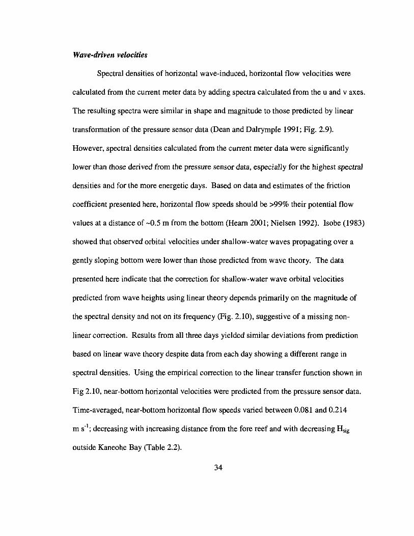
Wave-driven velocities

Spectral densities of horizontal wave-induced, horizontal flow velocities were

calculated from the current meter data by adding spectra calculated from the u and v axes.

The resulting spectra were similar in shape and magnitude to those predicted by linear

transformation of the pressure sensor data (Dean and Dalrymple 1991; Fig. 2.9).

However, spectral densities calculated from the current meter data were significantly

lower than those derived from the pressure sensor data, especially for the highest spectral

densities and for the more energetic days. Based on data and estimates of the friction

coefficient presented here, horizontal flow speeds should be >99% their potential flow

values at a distance of -0.5 m from the bottom (Heam 2001; Nielsen 1992). Isobe (1983)

showed that observed orbital velocities under shallow-water waves propagating over a

gently sloping bottom were lower than those predicted from wave theory. The data

presented here indicate that the correction for shallow-water wave orbital velocities

predicted from wave heights using linear theory depends primarily on the magnitude of

the spectral density and not on its frequency (Fig. 2.10), suggestive of a missing non­

linear correction. Results from all three days yielded similar deviations from prediction

based on linear wave theory despite data from each day showing a different range in

spectral densities. Using the empirical correction to the linear transfer function shown in

Fig 2.10, near-bottom horizontal velocities were predicted from the pressure sensor data.

Time-averaged, near-bottom horizontal flow speeds varied between 0.081 and 0.214

m S-I; decreasing with increasing distance from the fore reef and with decreasing Hsig

outside Kaneohe Bay (Table 2.2).

34

10.1 0.2 0.3 0.4 0.5 0.6 0.7 0.8 0.9

Frequency (HZ)

0.8

0.610Aug

0.4

0.2 ~,

"- ~"-

00 0.1 0.2 0.3 0.4 0.5 0.6 0.7 0.8 0.9 1

~

~

0.4,N:r:~ 0.3 16Aug

<nC'IE- 0.2>.~<nc 0.1Q)

Cl

~ 0.....U 0 0.1 0.2 0.3 0.4 0.5 0.6 0.7 0.8 0.9 1Q)0-

C/) 0.2

4Sep

0.1

Figure 2.9 Mean power spectral densities of near-bottom horizontal velocities for10 Aug, 16 Aug, and 4 Sep 2001 as measured directly with a 3D current meter(solid line) and predicted from pressure sensor measurements using lineartransformations (dashed line).

35

1.2

1.2

45ep

1.0

0.8 1.00.60.40.2

a =0.71b = 0.91r2 = 0.98N =3560

a = 0.74b = 0.91r2 =0.98N = 3870

a = 0.72b =0.94r2 = 0.99N =3827

1.2 f------,---,-------,-----,-------,---:;;'-'"

1.0

0.8

0.6

0.4

0.2 10 Aug

o~~=-------'-----'-----~--:'--~o 0.2 0.4 0.6 0.8 1.0 1.21.2 r-----r------,---,-------,---,---71

1.0

1.0

0.8

0.6

0.4

0.2

O-='-----L..----'-----_--L.-__-'--__-'-__--'o 0.2 0.4 0.6 0.8

'> 0.8::::l

; 0.6

.~ 0.4

~ 0.2 ~ !!"!~~~~:~~~'____~ __~1~6~A~U~9~~ 0 J..t5 0Q)Co 1.2 r-----r------,---,-------,---,----,71

(/)

..-.~

NI

N,IJl

N

E~

Spectral Density [P] (m2 s-2 Hz-1)

Figure 2.10 Power spectral densities for all frequencies from all bursts for 10Aug, 16 Aug, and 4 Sep 2001 as calculated from the current meter data [uvl andpredicted from the pressure data by linear transformation [Pl. The dashed linesrepresents a 1: 1 relationship. The solid lines represent a least-squares regressionof the form Y =aXb

• For data pooled from all three days, a =0.71 and b = 0.91(C =0.98, N = 11,257).

36

4 Aug 16 Aug 4Sep

Station Mean Range Mean Range Mean Range

1 0.214 0.191-0.233 0.164 0.133-0.185 0.116 0.100-0.131

2 0.167 0.147-0.188 0.148 0.104-0.179 0.119 0.099-0.136

3 0.126 0.107-0.126 0.137 0.092-0.162 0.086 0.062-0.112

4 0.119 0.098-0.139 0.102 0.058-0.132 0.081 0.057-0.104

Table 2.2 Mean and range (m S·I) of time-averaged, near-bottom horizontal flow

speeds (Uh)t for each day at each station. The ranges are given by the minimum

and maximum burst value from each deployment. Stations are ordered withincreasing distance from the fore reef (Fig. 2.3).

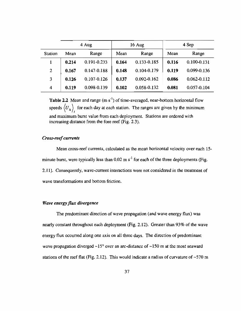
Cross-reefcurrents

Mean cross-reef currents, calculated as the mean horizontal velocity over each 15-

minute burst, were typically less than 0.02 m S·l for each of the three deployments (Fig.

2.11). Consequently, wave-current interactions were not considered in the treatment of

wave transformations and bottom friction.

Wave energy flux divergence

The predominant direction of wave propagation (and wave energy flux) was

nearly constant throughout each deployment (Fig. 2.12). Greater than 93% of the wave

energy flux occurred along one axis on all three days. The direction of predominant

wave propagation diverged -150 over an arc-distance of -150 m at the most seaward

stations of the reef flat (Fig. 2.12). This would indicate a radius of curvature of -570 m

37

0.04

0.030.020.01

0-0.01

-0.02-~•rnE'-'..... 0.04c~ 0.03....:::J 0.02u- 0.01(])(])

0....I

rn -0.01rn0 -0.02....Ucctl(])

::a:0.040.03

0.020.01

0-0.01-0.02

10Aug

15:00 18:00 21 :00 00:00 03:00 06:00 09:00

16Aug

12:00 15:00 18:00 21 :00 00:00 03:00 06:00

4Sep

15:00 18:00 21 :00 00:00 03:00 06:00 09:00

Time

Figure 2.11 Mean currents detennined from time-averaging of the current meterdata over each burst on 10 Aug, 16 Aug, and 4 Sep 2001.

38

15:00 18:00 21:00 00:00 03:00 06:00 09:00

4Sep

10Aug

16Aug

12:00 15:00 18:00 21 :00 00:00 03:00 06:00

15:00 18:00 21:00 00:00 03:00 06:00 09:00

mean = 2100

mean = 2250

mean =2170

230

228

226

224

222

220

-OlQ) 220"'C-c: 2180t5Q) 216....

"'Cx 214:::J

U. 212Q)>

~ 210

215

213

211

209

207

205

Figure 2.12 Principal direction of wave propagation determined from the currentmeter on 10 Aug, 16 Aug, 4 Sep 2001. The principal axis carried >93% of thevariance in flow speed on all three days.

39

in the shape of the propagating wave fronts. This is consistent with visual interpretation

of propagating wave fronts from an aerial photograph of the Kaneohe Bay Barrier Reef

which indicate a radius of curvature of -700 m near the most seaward stations and

decreasing towards the back of the reef flat (Fig. 2.4). Based on the above

considerations, R at the most seaward stations was taken to be equal to 630 m. Although

this method of estimating wave-energy flux divergence is simplistic, the data presented

here indicate that this process typically contributed at most 20-30% of the observed

decline in wave-energy fluxes across the study area (~ ).

Estimation ofCf

Since flow measurements were made only at the most seaward station of each

array, the time-averaged horizontal flow speed cubed, (Uh) t' was estimated from the

pressure sensor data using an empirical correction to the linear transfer function as

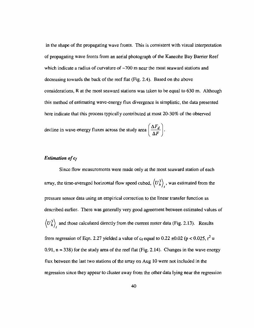
described earlier. There was generally very good agreement between estimated values of

(Uh), and those calculated directly from the current meter data (Fig. 2.13). Results

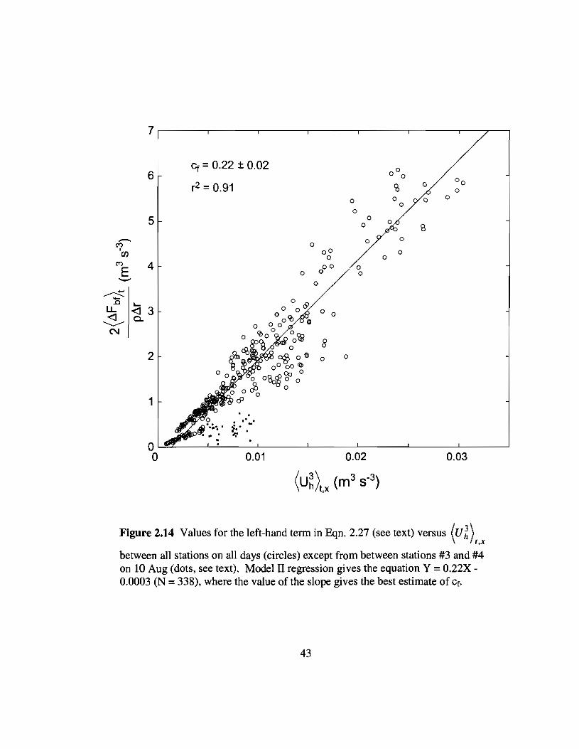
from regression of Eqn. 2.27 yielded a value of Cf equal to 0.22 ±O.02 (p < 0.025, ~ =

0.91, n = 338) for the study area of the reef flat (Fig. 2.14). Changes in the wave energy

flux between the last two stations of the array on Aug 10 were not included in the

regression since they appear to cluster away from the other data lying near the regression

40

0.04 r2 =0.99 ••n =126 • •,

• •• ••... •0.03 • ••

..-.. ...•C"'l •,l/) ••

C"'l

E •••- •...... •a.. 0.02 •...... ••- .,/\ •, '..<:::: ••::::l ,,).V I: .

0.01 ...•,

0.040.030.020.01o "'--- -'-- -'-- ----'- ----L_---.J

o

Figure 2.13 Time-averaged near-bottom horizontal flow speeds cubed aspredicted and corrected from sensor data [P] and as directly computed fromcurrent meter data [uv]. The solid line represents a 1:1 relationship.

line. This is likely due to non-local inputs of wave energy from the area of the Kaneohe

Bay Barrier Reef northwest of Kapapa Island on this most energetic day. The northwest

haIf of the reef flat is deeper (2-3 m) than areas of the reef flat southeast of Kapapa Island

and could have allowed for the transmission of wave energy to the most landward station

41

where observed wave energy densities would be higher than expected. Separation of the

data from all three days into three pairs of stations with increasing distance from the fore

reef indicated that Cf did not vary significantly with distance across the study area (p <

0.025). Uncertainty in the estimate of Cf for the reef flat community can also come from

uncertainty in the radii of curvature for the diverging wave fronts (Eqns. 2.17 & 2.18).

However, an uncertainty of ± 200 m in the radii of curvature estimated here translates

into an equivalent uncertainty of only ± 5% in the value of Cr, or ± 0.01. Consequently,

the uncertainty in Cr is ± 0.03 or:t 14%.

Estimation ofk based on cf

Estimates of k based on Cf can be obtained from the literature on turbulent,

oscillatory flow over rough surfaces. Reef communities are typically heterogeneous

surfaces lacking a singular roughness scale. For this reason, the roughness height, k, was

derived from estimates of Cf. Flow conditions across the study area met the criteria for

rough, turbulent, oscillatory (Kamphuis 1975) based on the estimated friction factors and

relevant Reynolds numbers. Nielsen (1992) reanalyzed various experimental data on the

friction generated by oscillatory flow over rough surfaces (Jensen 1989; Kemp and

Simons 1983; Riedel 1972; Sleath 1987; Swart 1974) and gave the following empirical

expression

(2.28)

42

7

6ct =0.22 ± 0.02

000

00r2 =0.91 '0 0

0

0 0 0 00

0

5 000 \>

~ 0 0

"" 0,00 0en 0 0

"" 4 00E 0

0 0 0'-'"

0

~- 0.c .... o 06'U. -<I 3 0-<I 0 0c- olO 0

---------0 00

N 0'<>0 o~o 0 0

<it,8O'fj 0 0

2 ~'d> '1> 00 0 0

0°00 (Q)o 00 0

o 0 0?b8 0 0

oJ; 0

1o 0

c9

" ,i· .., ,"

00 0.01 0.02 0.03

\U~)tx (m38.

3),

Figure 2.14 Values for the left-hand term in Eqn. 2.27 (see text) versus (U~)I.x

between all stations on all days (circles) except from between stations #3 and #4on 10 Aug (dots, see text). Model II regression gives the equation Y = 0.22X­0.0003 (N = 338), where the value of the slope gives the best estimate of Cf.

43

where k is the roughness height as described before, A is the horizontal orbital excursion

amplitude, and fw is the friction factor relating the maximum shear stress to Um2

• For

simple harmonic flows, the exact relationship between fw and fe (Kajiura 1968) is

(2.29) = 1.( 8 ), 3Jl"cos¢

where the ratio in parentheses is"" 1, given a value of <p "" 25° cited earlier. Furthermore,

the literature review by Nielsen (1992) revealed that fw "" fe for turbulent, oscillatory flow

over rough bottoms within the variability of experimental data. For the present purposes

I will thus consider that Cf"" fw "" fe• Kamphuis (1975) also gave an expression to obtain

fw for the conditions of A!k :::: 100 which apply here

(2.30) (k )0.75

= 0.4 ­A

Based on the data presented here, fw as estimated by Eqn. 2.30 should also be between

0.10 and 0.40. Nelson (1996) used a relationship similar to that of Eqn. 2.28 (Swart

1974) to estimate the average roughness height of a shallow reef from values of fe•

For the data presented here, the rms-orbital amplitude, Arm" varied from 0.2 m at

the most back-reef stations to 0.6 m at the most fore-reef stations. Using the value of Cf

estimated before and a mean Arms of 0.4 m for the study area, we get an average k for

the study area of 0.20 m from Eqn. 2.28 and 0.18 m from Eqn. 2.30. Based on these

results, a value of 0.2 m was chosen to represent the roughness height of this reef flat

community. This values is consistent with observations of roughness height made in the

field.

44

Estimates ofnutrient mass transfer coefficknts

S was calculated based on the regression shown in Fig. 2.1. This assumes that

the mass transfer relationship is the same under steady and oscillatory flow. Mean values

for the nutrient mass transfer coefficient, Si, across the study area were estimated for each

station over the entire duration of each deployment (Table 2.3). The relationship in Eqn.

2.12 assumes that S is proportional to UhO.8, therefore, the time-averaged values ofUho.8

were used to estimate mean values for S. Estimates of S for phosphate, Sp, ranged

between 3.6 and 7.1 m dai1 while values of S for both ammonium and nitrate, SN, varied

between 5.9 and 12.0 m dai1• By Eqn. 2.12, the reported uncertainty in Cf would

translate into an uncertainty in S of only about ± 5%. Uncertainty in estimates of S

resulting from the regression shown in Fig. 2.1, based on 95% confidence limits, are

about ± 0.5 m dail for dissolved phosphate and:!: 0.7 m dai1 for ammonium and nitrate.

Given that mean significant wave heights outside the bay were 2.0 m over a two-year

period, I will consider the conditions on 10 Aug to be representative of average nutrient

mass transfer coefficients for that particular reef flat community. Using a mean (Uh)t

over all stations from this day alone gives an average Sp equal to 5.8 ± 0.8 m dai1 and SN

equal to 9.7 ± 1.3 m day' I.

45

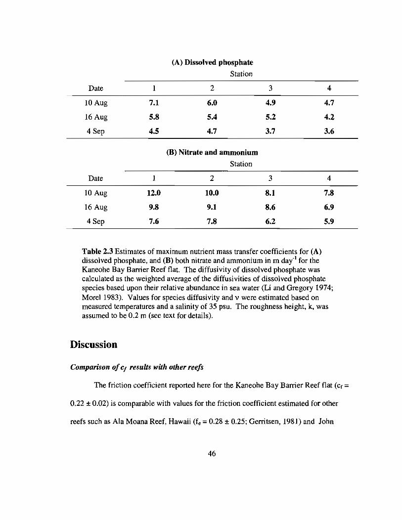
(A) Dissolved phosphate

Station

Date I 2 3 4

10 Aug 7.1 6.0 4.9 4.7

16 Aug 5.8 5.4 5.2 4.2

4Sep 4.5 4.7 3.7 3.6

(B) Nitrate and ammonium

Station

Date I 2 3 4

10 Aug 12.0 10.0 8.1 7.8

16 Aug 9.8 9.1 8.6 6.9

4Sep 7.6 7.8 6.2 5.9

Table 2.3 Estimates of maximum nutrient mass transfer coefficients for (A)dissolved phosphate, and (B) both nitrate and ammonium in m dai1 for theKaneohe Bay Barrier Reef flat. The diffusivity of dissolved phosphate wascalculated as the weighted average of the diffusivities of dissolved phosphatespecies based upon their relative abundance in sea water (Li and Gregory 1974;Morel 1983). Values for species diffusivity and v were estimated based onmeasured temperatures and a salinity of 35 psu. The roughness height, k, wasassumed to be 0.2 m (see text for details).

Discussion

Comparison ofCf results with other reefs

The friction coefficient reported here for the Kaneohe Bay Barrier Reef flat (Cf =

0.22 ± 0.02) is comparable with values for the friction coefficient estimated for other

reefs such as Ala Moana Reef, Hawaii (fe = 0.28 ± 0.25; Gerritsen, 1981) and John

46

Brewer Reef, Great Barrier Reef (fe '" 0.15 ± 0.04; Nelson, 1996). Each of these average

values is close to the proposed asymptotic limits for the value of fe (0.25-0.30) mentioned

earlier. Estimates of k derived from Eqns. 2.28 & 2.30 are similar to visual estimates

made in the field and correspond to values of AIk '" 2. Kajiura (1968) proposed a

theoretical limit offw '" 0.25 for AIk < 1.67. However, in reviewing a greater number of

experimental data sets, Jonsson (1980) indicated that a constant value of fw '" 0.30 should

be used for Afk < 1.57. Both of these results can explain why the estimate of Cf reported

here is close to this asymptotic limit; i.e., of order 0.1 as opposed to order 0.01. It can

also explain why Cf did not vary significantly across the study area (p < 0.025). The

comparably high values of fe or Cf for different reefs may result from the magnitude of

their roughness heights being of similar scale to wave orbital excursion amplitudes.

More data will need to be collected before generalizations on the high frictional

roughness of reef communities under waves can be made.

Past estimates ofS

Bilger and Atkinson (1992) underestimated Cf for the same Kaneohe Bay Barrier

Reef flat community a factor of 10-20 lower as compared with the present estimate of Cf.

This discrepancy translates into estimates of 5t and 5 that are a factor of 2.5-3.3 lower

than estimated here. In a paper contemporary with Bilger and Atkinson (1992), Atkinson

(1992) estimated the rate of phosphate uptake for two windward Enewetak Atoll reef flats

based on mass transfer correlations using a value of Cf which was a factor of 10-20 times

lower than that of the Kaneohe Bay Barrier Reef flat and other reefs (Gerritsen 1981;

47

Nelson 1996). The much greater ability for coral reef communities to transfer

momentum (i.e., higher friction coefficients) than previously known by coral reef

biogeochemists implies a greater ability to transfer mass. Bilger and Atkinson (1992) did

not have any measurements of flow velocities across the Kaneohe Bay Barrier Reef flat

available to them and used an average velocity of 0.06 m S-I in their calculations based on

prior estimates of cross-reef transports (Atkinson 1987a; Bathen 1968). This is much

lower than typical horizontal flow speeds measured here. The authors estimated average

flow speeds induced by the passage of a O.S-m solitary wave and estimated a value of

0.19 m sot, however, they only suggested that "wave surge" may be an important source

of mass transfer enhancement. Furthermore, it is clear that flow velocities across the

Kaneohe Bay Barrier Reef flat cannot be characterized by a single velocity scale derived

from a single wave form. Atkinson (1992) had unpublished velocity and depth data for

his calculations, but did not report any information regarding the spatial and temporal

variability in these measurements, nor how they were collected.

Variations in S driven by wave transformation

Changes in Cf across the study area were not significant (p < 0.025). Furthermore,

S depends on Cf only to the 0.4 power (Eqn. 2.12). Therefore, spatial and temporal

variation in S across the study area should result primarily from variations in horizontal

flow speed (Uh, Eqn. 2.12, Table 2.2). Spatial variations in Uh across the reef flat are

driven by attenuation of residual waves moving out of the surf zone (Table 2.1 & 2.2).

48

Because most reef flats lie behind a breaking zone, the wave environment over

most reef flats will be influenced by the wave breaking process. In the simplest

description of depth-induced breaking, waves of a given height break when they exceed

some fraction (y) of the water depth, h (Dean and Dalrymple 1991; Horikawa 1988)

(2.31) HJllID( = yh

The effect of depth-induced breaking is similar to that of an amplitude filter, reducing the

height of waves which exceed the maximum allowable height. Wave breaking was

observed to occur continuously on all three days, yet Hrms and Vh varied between days

according to the mean significant wave height outside Kaneohe Bay (Tables 2.1 & 2.2).

This indicates that the average height of residual waves propagating from the surf zone

are still influenced by the height of waves outside the breaking zone despite the

amplitude-filtering effects of depth-induced breaking. Therefore, temporal variations in

S across the reef flat are still influenced by variation in wave heights outside Kaneohe

Bay, albeit substantially damped by the wave breaking process.

The height of residual waves propagating from the surf zone can also be

modulated by tidal changes in water depth (Fig. 2.8, Table 2.1). Such tidal regulation of

wave transformation and attenuation near coral reefs has been documented elsewhere

(Lugo-Fernandez et al. 1998a, 1998b). Tidally induced variations in Hrms across the reef

flat were relatively greater than variations in Vh (Tables 2.1 & 2.2). This is because

shallow-water wave-orbital velocities are proportional to wave height, but inversely

proportional to the square root of the water depth according to linear approximation

49

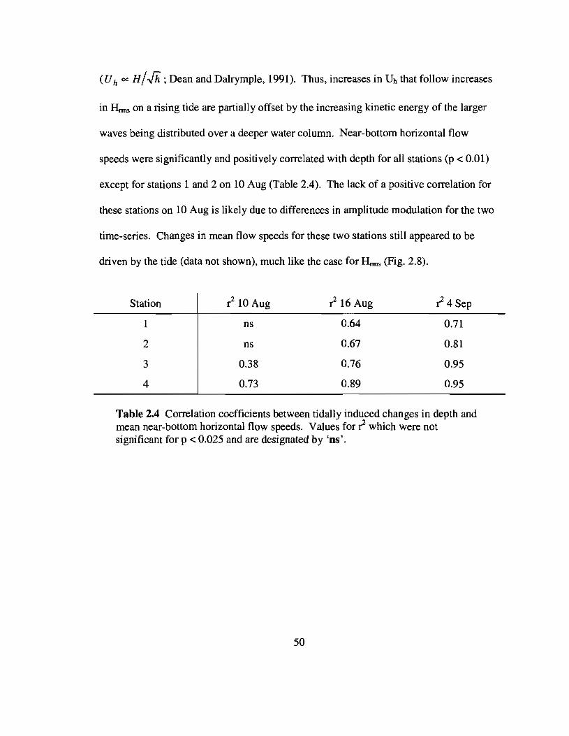
( Uh <X H/.Jh ;Dean and Dalrymple, 1991). Thus, increases in Dh that follow increases

in Hnru; on a rising tide are partially offset by the increasing kinetic energy of the larger

waves being distributed over a deeper water column. Near-bottom horizontal flow

speeds were significantly and positively correlated with depth for all stations (p < 0.01)

except for stations I and 2 on 10 Aug (Table 2.4). The lack of a positive correlation for

these stations on 10 Aug is likely due to differences in amplitude modulation for the two

time-series. Changes in mean flow speeds for these two stations still appeared to be

driven by the tide (data not shown), much like the case for H.ms (Fig. 2.8).

Station r2 10 Aug r2 16 Aug C4Sep

1 ns 0.64 0.71

2 ns 0.67 0.81

3 0.38 0.76 0.95

4 0.73 0.89 0.95

Table 2.4 Correlation coefficients between tidally induced changes in depth andmean near-bottom horizontal flow speeds. Values for C which were notsignificant for p < 0.025 and are designated by 'os'.

50

III

NUTRIENT MASS TRANSFER RATES DERIVED FROM

THE DISSOLUTION OF PLASTER MOLDS

Introduction

Chapter goals

The first goal of this chapter is to use the dissolution of plaster molds to provide

estimates of nutrient mass transfer coefficients for a Kaneohe Bay Barrier Reef flat

community. The second goal of the chapter is to examine the importance of different

roughness scales relevant to coral reef communities (0.001 - 0.1 m) on rates of nutrient

mass transfer for a given surface. The third goal is to determine whether there is a

significant difference between rates of nutrient mass transfer under the steady flow

conditions of an experimental flume used in prior mass transfer experiments with the in

situ, wave-driven flows to which natural reef communities are exposed.

Bcu:kground: The utility ofdissolving piaster surfcu:es

The dissolution of plaster, or gypsum (CaS04'2H20), is widely used in aquatic

sciences to characterize water motion because plaster forms have been shown to dissolve

faster at higher flow speeds (Muus 1968; Doty 1971; Thompson and Glenn 1994;

51

Santschi et al. 1991; Jokiel and Morrisey 1993; Porter et al. 2000). These observations

can be explained by mass transfer theory. Baird and Atkinson (1997) showed that mass

transfer correlations could accurately predict rates of dissolution of gypsum-coated corals

in experimental communities once the flow velocity and frictional characteristics of the

community were known. In an earlier work, Thomas and Atkinson (/997) showed that

mass transfer correlations could accurately predict rates of ammonium uptake by

experimental communities of coral and turf-covered coral rubble which varied in relief

and frictional roughness. The agreement between these two studies demonstrated how

the dissolution of plaster surfaces could be used to describe the mass transfer of nutrients.

This is because the diffusivities ofthe major ions in gypsum (Ca2+ and SOl') and

dissolved inorganic nutrient species (e.g., polo, HPo/', NH/, and N03') are of the same

scale (Li and Gregory 1974).

Methods

The basic approach was to 1) fabricate plaster (gypsum) surfaces of varying

morphological character, 2) deploy these molds under different flow conditions, 3)

estimate the rate of mass transfer from the mold by measuring changes in the weight of

the plaster mold before and after a deployment, and 4) compare these rates with mold

surface areas.

52

Plaster mold design

Plaster molds were constructed using rectangular plaster forms, or elements, of

square cross-sectional area (6.1 x6.l cm2). Anywhere from 8 to 22 of these forms, 4-15

cm in height, were placed upright on a tray made from 0.32 cm-thick sheet aluminum.

The sides of the tray were -2-2.5 cm high and were easily formed by bending the

aluminum sheet in a vise to form right angles. The purpose of these sides were three­

fold: I) to give the light aluminum tray more strength, 2) to provide a reservoir into

which additional plaster could be poured, thus creating a surface entirely made of plaster,

and 3) to help secure the individual elements in place and reduce the fragility of the entire

mold. Two sizes of square aluminum trays were used throughout this study: one set

0.5xO.5 m and another set 0.38xO.38 m. The reason for the change in tray size was to

create molds that could be deployed inside a re-circulating flume as well as in the field.

Three threaded, stainless steel rods (lOx 1.3 cm) were used as bolts to hold two anchor

bars to the bottom of the tray (Fig. 3.1A). The anchors were made from 1X 10 cm mild

steel bar. The threaded rods extended -5 cm below the anchors, forming legs for the

plaster mold. The extension of the bolts allowed the mold and anchors to sit above any

roughness < 5 cm in the field. PVC irrigation pipe 2.3 cm in diameter dammed each bolt

hole from plaster being poured into the tray and were sealed to the tray with silicone.

Plaster elements and molds were prepared using US Gypsum (Chicago, Illinois,

USA) No.1 pottery plaster (% by weight: 96.2% 13-hemihydrate [CaS04'1/2HzOl, 0.5%

CaS04, 2.4% dolomite [CaMg(C03hl, 0.4% oxides, 0.5% acid insolubles). This

composition was checked against an analysis of the material by inductively coupled

53

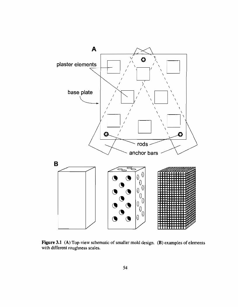
A

plaster elements~---1-+-

base plate

~

rods

anchor bars

B.-/

Figure 3.1 (A) Top-view schematic of smaller mold design. (B) examples of elementswith different roughness scales.

54

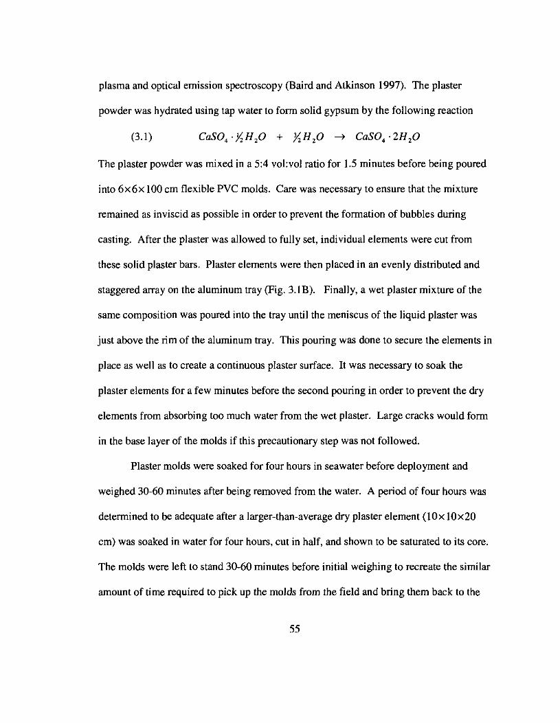
plasma and optical emission spectroscopy (Baird and Atkinson 1997). The plaster

powder was hydrated using tap water to fonn solid gypsum by the following reaction

(3.1) CaS04 ·Y,H,G + Y,H 20 ~ CaSO.·2H20

The plaster powder was mixed in a 5:4 vol:vol ratio for 1.5 minutes before being poured

into 6x6x 100 cm flexible PVC molds. Care was necessary to ensure that the mixture

remained as inviscid as possible in order to prevent the fonnation of bubbles during

casting. After the plaster was allowed to fully set, individual elements were cut from

these solid plaster bars. Plaster elements were then placed in an evenly distributed and

staggered array on the aluminum tray (Fig. 3.1B). Finally, a wet plaster mixture of the

same composition was poured into the tray until the meniscus of the liquid plaster was

just above the rim of the aluminum tray. This pouring was done to secure the elements in

place as well as to create a continuous plaster surface. It was necessary to soak the

plaster elements for a few minutes before the second pouring in order to prevent the dry

elements from absorbing too much water from the wet plaster. Large cracks would fonn

in the base layer of the molds if this precautionary step was not followed.

Plaster molds were soaked for four hours in seawater before deployment and

weighed 30-60 minutes after being removed from the water. A period of four hours was

detennined to be adequate after a larger-than-average dry plaster element (lOX lOx20

cm) was soaked in water for four hours, cut in half, and shown to be saturated to its core.

The molds were left to stand 30-60 minutes before initial weighing to recreate the similar

amount of time required to pick up the molds from the field and bring them back to the

55

Hawaii Institute of Marine Biology by boat. Each mold weighed between 8-20 kg, with

typical weight losses over a deployment varying between 0.5 and 2 kg, or -5-10% of the

wet weight of the molds.

To convert weight loss of wet plaster to loss of calcium in moles, an experiment

was performed to determine the ratio between the densities of dry and wet plaster

(Pdr/Pwe,). Three batches of plaster were separately prepared in the same way as for the

molds. The liquid plaster from each batch was poured into two 0.5-L plastic cups

approximately 8 cm in diameter and 12 cm high and allowed to sit overnight. The

following day all six solid plaster forms were soaked in water for four hours, allowed to

sit for 30 minutes, and then weighed before being placed in a temperature-controlled

oven at 55°C. The forms were then weighed four times over the following four days after

which Pdr/Pwet had reached an equilibrium value of 0.64 ± 0.02 (Fig. 3.2). The weight

of plaster lost from a mold over the duration of a deployment (/1Wwet) could then be

converted into the mass of calcium lost (!!.Mea) by the following equation

(3.2) A II _ /1Wwet (Pd'Y)UlYlCa - --

MWgyp Pwet

where MWgyp is the molecular weight of gypsum (172.1 g).

56

10,UG--------,-----,r-----,------.----,--------,-------,

o batch 1'V batch 2o batch 3

90

.......c

80OJ.~

ctlEc

:;,R. 700

B B- - - - - -- - - - - - - _:--:_~~----~

60

50 L-__L-__-'--__.l.--__--'---__---'---__---"---__---.J

o 20 40 60 80 100 120 140

Time (hours)

Figure 3.2 Change in density of plaster elements with time following drying inan oven at 55·C.

Mass transfer ofcrl+ from dissolving gypsum surfaces

The simplest mass transfer formulation relates the flux of a species, Ji, from a

surface to the difference between the concentration of that species in the ambient fluid,

Ci,b, and adjacent to the surface, Ci,w, by the mass transfer coefficient, Sj

57

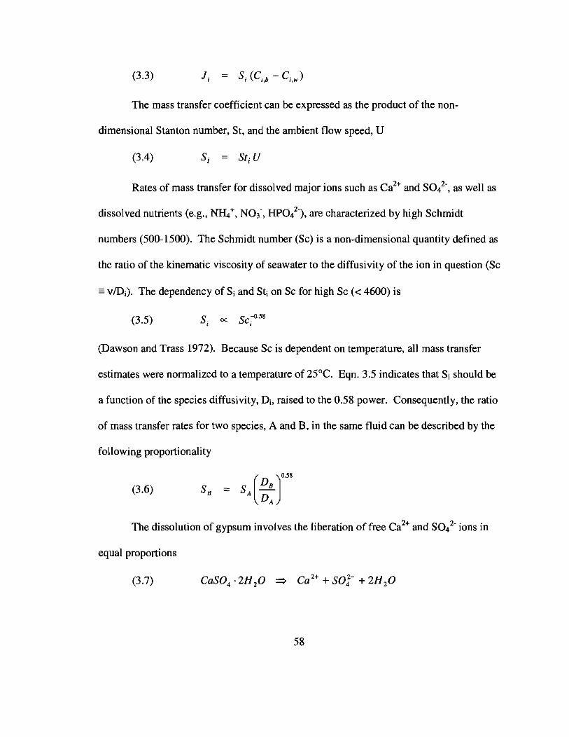
(3.3) J, = S, (C, .• - C,.• )

The mass transfer coefficient can be expressed as the product of the non-

dimensional Stanton number, St, and the ambient flow speed, U

(3.4) Sj = Sfi U

Rates of mass transfer for dissolved major ions such as Ca2+ and sol', as well as

dissolved nutrients (e.g., NHt, NOl', HPO/'), are characterized by high Schmidt

numbers (500-1500), The Schmidt number (Sc) is a non-dimensional quantity defined as

the ratio of the kinematic viscosity of seawater to the diffusivity of the ion in question (Sc

== vlDj). The dependency of Sj and Sti on Sc for high Sc « 4600) is

(3.5) S cc Sc:".58, ,

(Dawson and Trass 1972), Because Sc is dependent on temperature, all mass transfer

estimates were normalized to a temperature of 25 DC, Eqn, 3.5 indicates that Si should be

a function of the species diffusivity, Di, raised to the 0.58 power. Consequently, the ratio

of mass transfer rates for two species, A and B, in the same fluid can be described by the

following proportionality

( JO.58

(3.6) SB = SA ~:

The dissolution of gypsum involves the liberation offree Ca2+ and sol' ions in

equal proportions

(3.7) CaSO• .2H,o ~ Ca 2+ + SO;- + 2H,o

58

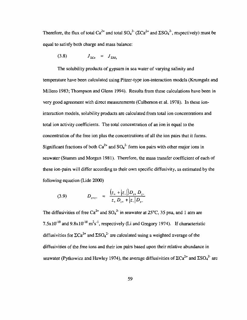
Therefore, the flux of total Ca2+ and total sol' (:ECa2+ and :ESOl', respectively) must be

equal to satisfy both charge and mass balance:

(3.8)

The solubility products of gypsum in sea water of varying salinity and

temperature have been calculated using Pitzer-type ion-interaction models (Krumgalz and

Millero 1983; Thompson and Glenn 1994). Results from these calculations have been in

very good agreement with direct measurements (Culberson et al. 1978). In these ion-

interaction models, solubility products are calculated from total ion concentrations and

total ion activity coefficients. The total concentration of an ion is equal to the

concentration of the free ion plus the concentrations of all the ion pairs that it forms.

Significant fractions of both Ca2+ and sol' form ion pairs with other major ions in

seawater (Stumm and Morgan 1981). Therefore, the mass transfer coefficient of each of

these ion-pairs will differ according to their own specific diffusivity, as estimated by the

following equation (Lide 2000)

(3.9) D z+z- ==(z+ + Iz.I)D,+ D,.

z+ D,+ +Iz.ID,.

The diffusivities of free Ca2+ and S042' in seawater at 2YC, 35 psu, and 1 atm are

7.5xlO'lO and 9.8xlO'lO m2s'I, respectively (Li and Gregory 1974). If characteristic

diffusivities for :ECa2+ and :ESOl' are calculated using a weighted average of the

diffusivities of the free ions and their ion pairs based upon their relative abundance in

seawater (Pytkowicz and Hawley 1974), the average diffusivities of:ECa2+ and :ESOl' are

59

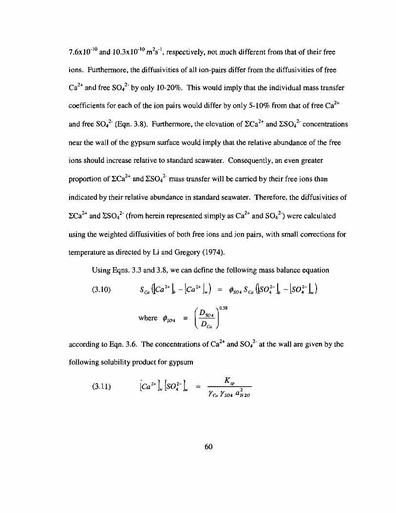
7.6xlO-1O and 1O.3xlO-1o m2s-1, respectively, not much different from that of their free

ions. Furthermore, the diffusivities of all ion-pairs differ from the diffusivities of free

Ca2+and free sol- by only 10-20%. This would imply that the individual mass transfer

coefficients for each of the ion pairs would differ by only 5-10% from that of free Ca2+

and free sol- (Eqn. 3.8). Furthermore, the elevation of ~Ca2+ and ~sol- concentrations

near the wall of the gypsum surface would imply that the relative abundance of the free

ions should increase relative to standard seawater. Consequently, an even greater

proportion of ~Ca2+ and ~solmass transfer will be carried by their free ions than

indicated by their relative abundance in standard seawater. Therefore, the diffusivities of

~Ca2+ and ~sol- (from herein represented simply as Ca2+and sol") were calculated

using the weighted diffusivities of both free ions and ion pairs, with small corrections for

temperature as directed by Li and Gregory (1974).

Using Eqns. 3.3 and 3.8, we can define the following mass balance equation

(3.10)

where i/JS0 4( )

0.58Dso4= --DCa

according to Eqn. 3.6. The concentrations of Ca2+ and sol- at the wall are given by the

following solubility product for gypsum

(3.11) [Ca 2+L[so;-L2

YCa YS04 aH20

60

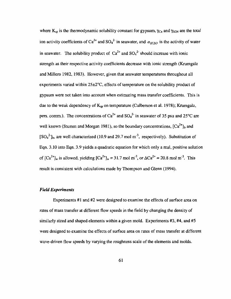
where Ksp is the thermodynamic solubility constant for gypsum, YCa and YS04 are the total

ion activity coefficients of Ca2+ and sol- in seawater, and aH20 is the activity of water

in seawater. The solubility product of Ca2+ and sol' should increase with ionic

strength as their respective activity coefficients decrease with ionic strength (Krumgalz

and Millero 1982, 1983). However, given that seawater temperatures throughout all

experiments varied within 25±2°C, effects of temperature on the solubility product of

gypsum were not taken into account when estimating mass transfer coefficients. This is

due to the weak dependency of Ksp on temperature (Culberson et aI. 1978); Krurngalz,

pers. comm.). The concentrations of Ca2+ and sol' in seawater of 35 psu and 25°C are

well known (Stumm and Morgan 1981), so the boundary concentrations, [Ca2+]b and

[SO/h, are well characterized (10.9 and 29.7 mol m-3, respectively). Substitution of

Eqn. 3.10 into Eqn. 3.9 yields a quadratic equation for which only a real, positive solution

of [Ca2+]w is allowed, yielding [Ci+]w =31.7 mol m-3, or <1Ca2+ =20.8 mol m-3

• This

result is consistent with calculations made by Thompson and Glenn (1994).

Field Experiments

Experiments #1 and #2 were designed to examine the effects of surface area on

rates of mass transfer at different flow speeds in the field by changing the density of

similarly sized and shaped elements within a given mold. Experiments #3, #4, and #5

were designed to examine the effects of surface area on rates of mass transfer at different

wave-driven flow speeds by varying the roughness scale of the elements and molds.

61

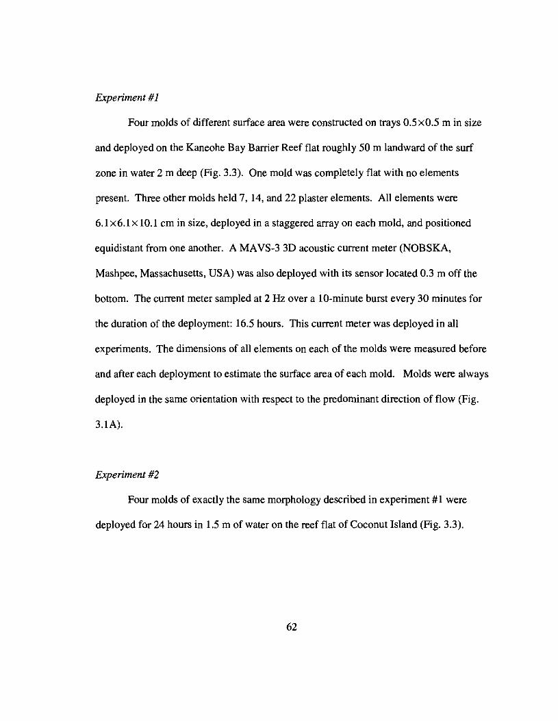
Experiment #1

Four molds of different surface area were constructed on trays 0.5 xO.5 m in size

and deployed on the Kaneohe Bay Barrier Reef flat roughly 50 m landward of the surf

zone in water 2 m deep (Fig. 3.3). One mold was completely flat with no elements

present. Three other molds held 7, 14, and 22 plaster elements. All elements were

6.1 x6.1 x 10.1 em in size, deployed in a staggered array on each mold, and positioned

equidistant from one another. A MAVS-3 3D acoustic current meter (NOBSKA,

Mashpee, Massachusetts, USA) was also deployed with its sensor located 0.3 m off the

bottom. The current meter sampled at 2 Hz over a lO-minute burst every 30 minutes for

the duration of the deployment: 16.5 hours. This current meter was deployed in all

experiments. The dimensions of all elements on each of the molds were measured before

and after each deployment to estimate the surface area of each mold. Molds were always

deployed in the same orientation with respect to the predominant direction of flow (Fig.

3.1A).

Experiment #2

Four molds of exactly the same morphology described in experiment #1 were

deployed for 24 hours in 1.5 m of water on the reef flat of Coconut Island (Fig. 3.3).

62

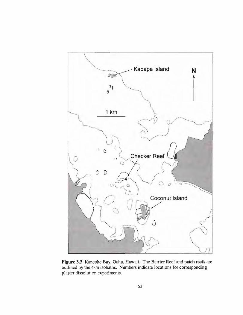
Kapapa Island N

1 km

o ()

oo

o D

a

G

6 0

Coconut Island

2/

o

Figure 3.3 Kaneohe Bay, Oahu, Hawaii. The Barrier Reef and patch reefs areoutlined by the 4-m isobaths. Numbers indicate locations for correspondingplaster dissolution experiments.

63

Experiment #3

Three molds were deployed for roughly 7 hours in the same area of the Kaneohe

Bay Barrier Reef flat as in experiment 1 (Fig. 3.3). One mold was flat with no elements

and the other two molds each held 14 elements 6.1 x6.l x 14.8 cm in size. 61 holes l-cm

in diameter and approximately 1 cm deep were drilled in a staggered fashion on all faces

of all of the elements on one of the molds (similar to the example shown in Fig. 3.1B),

yielding 854 holes in total. These holes added surface area to the mold by giving the

mold an additional roughness scale on the order of 1 cm. 40-60 measurements of hole

depth and diameter were measured at random with a set of calipers before and after

deployment to estimate the amount of surface area added to the molds by the holes.

Experiment #4

Four large molds and two pairs of individual elements were deployed under mild

trade wind conditions on the reef flat of Checker Reef (Fig. 3.3), a patch reef protected

from ocean swell. All trays were 0.38xO.38 m in size. The first mold was flat, while the

next three molds each had 8 elements arranged in a pattern as shown in Fig. 3.1A.

Elements on the second mold were 6.1x6.1x4.8 em and had smooth faces. Elements on

the third mold were 6.1 x6.1 x 12.5 em and also had smooth faces. Elements on the fourth

mold were 6.1 x6.1x 12.5 em, but with l.1-cm wide and l.1-cm deep holes drilled into

the faces of all the elements, producing 384 holes (8x48) in total (Fig. 3.1B). Two pairs

of individual elements were deployed along with the larger molds. One element of each

pair had smooth faces and was 12.1 em in height. The other element in each pair was

64

also 12.1 em high, but had grooves -2-mm deep and -1.5-mm wide carved in it at

intervals of every 5 mm so that a grid-like pattern with over 1000 facets on each grooved

element was formed (Fig. 3.lB). These grooves added surface area to the mold by

providing an additional roughness scale of -2 mm.

Grooved elements were deployed individually rather than in a group on a larger

mold for two reasons. First, these elements would only allow for relatively small

changes in weight before their mm-scale surface features would disappear. Thus, these

elements were deployed for shorter periods of time than other molds. The second reason

was that the construction of larger molds from grooved elements required much more

preparation time than other molds and, thus, were not considered worthwhile. Since the

number of grooves and facets were large, only 40-50 measurements of groove depth and

width before and after deployment were made to estimate total surface added to the

elements by the grooves. In order to compare results from the dissolution of individual

elements with those of the molds, I calculated the surface area a mold would have if

constructed from these individual elements. The ratio between this extrapolated area and

the actual surface area of the individual elements was then multiplied by the weight loss

of the individual elements to get a weight loss equivalent to that of an entire mold.

Experiment #5

Molds similar to those used in experiment #4 were deployed on the Kaneohe Bay

Barrier Reef flat under moderate wave conditions roughly 100 m landward of the surf

65

zone (Fig. 3.3). One of the individual smooth elements was replaced by an element of

similar size, but with holes drilled in it as described earlier (Fig. 3.IB).

Flume experiments

Experiments #1 and #3 on the Kaneohe Bay Barrier Reef flat showed the

dependence of rates of mass transfer for fabricated gypsum molds on surface area under

dominantly oscillatory flow conditions with mean flow speeds of around 0.2 m s".

Therefore, molds of varying roughness scale and total surface area, similar to those used

in field experiments, were placed in an advective, re-circulating flume to directly

compare rates of mass transfer for these forms in the flume with those obtained in the

field. The experimental flume used here has been described more thoroughly elsewhere

(Atkinson and Bilger 1992; Baird and Atkinson 1997). Briefly, it consisted of two

channels 0.4 m wide, 0.3 m deep, and 9 m long connected by 1800 turns at either end.

Five molds 0.38xO.38 m were used, along with two pairs of individual elements (one

grooved, one smooth) as described earlier for experiment #4.

During the flume experiments, only one mold was deployed at a given time. A

MAVS-3 current meter was placed with only its sensor in the flume to measure flow

speeds (Fig. 3.4). These measurements were checked against flow speed measurements

estimated from the time required for a neutrally buoyant 500-mL plastic bottle -0.2 m

high, acting as a drogue, to pass a given distance within the flume. Because the size of

the molds were significant with respect to the dimensions of the flume, the presence of

the molds and element pairs represented a 15-30% decrease in the flow cross-sectional

66

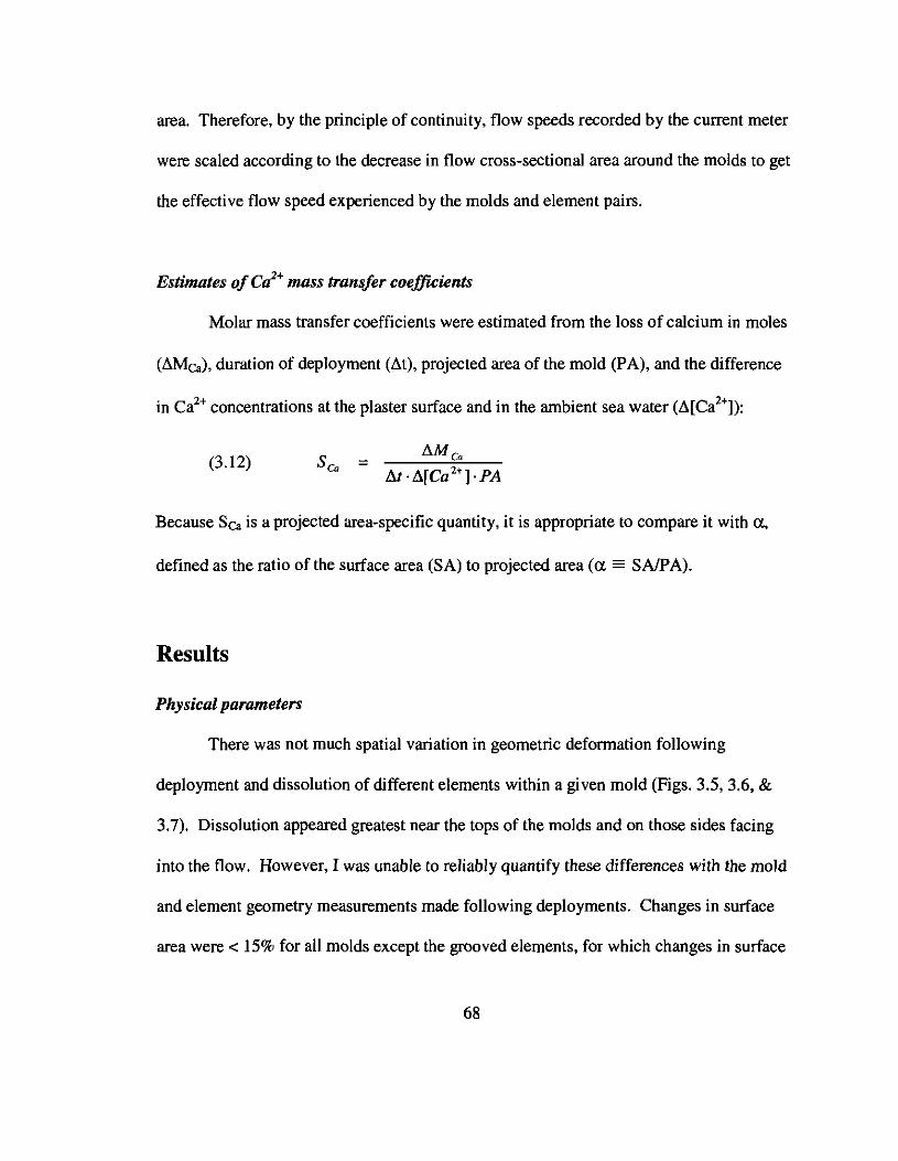
area. Therefore, by the principle of continuity, flow speeds recorded by the current meter

were scaled according to the decrease in flow cross-sectional area around the molds to get

the effective flow speed experienced by the molds and element pairs.

Estimates ofctl+ mass transfer coefficients

Molar mass transfer coefficients were estimated from the loss of calcium in moles

(tl.Mea), duration of deployment (tl.t), projected area of the mold (PA), and the difference

in Ca2+ concentrations at the plaster surface and in the ambient sea water (L'.[Ca2+]):

(3.12) =t1Mc,

Because Sea is a projected area-specific quantity, it is appropriate to compare it with a,

defined as the ratio of the surface area (SA) to projected area (a. =SAJPA).

Results

Physical parameters

There was not much spatial variation in geometric deformation following

deployment and dissolution of different elements within a given mold (Figs. 3.5, 3.6, &

3.7). Dissolution appeared greatest near the tops of the molds and on those sides facing

into the flow. However, I was unable to reliably quantify these differences with the mold

and element geometry measurements made following deployments. Changes in surface

area were < 15% for all molds except the grooved elements, for which changes in surface

68

Figure 3.4 Experimental setup for the dissolution of plaster molds in a re­circulating flume. The mold shown is 7.5 m downstream from the opposite end ofthe flume. The current meter is shown wrapped in a white towel to prevent itfrom overheating in the sun. A meter stick lying along the right-hand side of theflume is provided for scale.

67

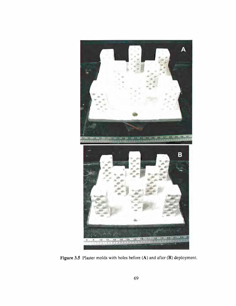
Figure 3.5 Plaster molds with holes before (A) and after (B) deployment.

69

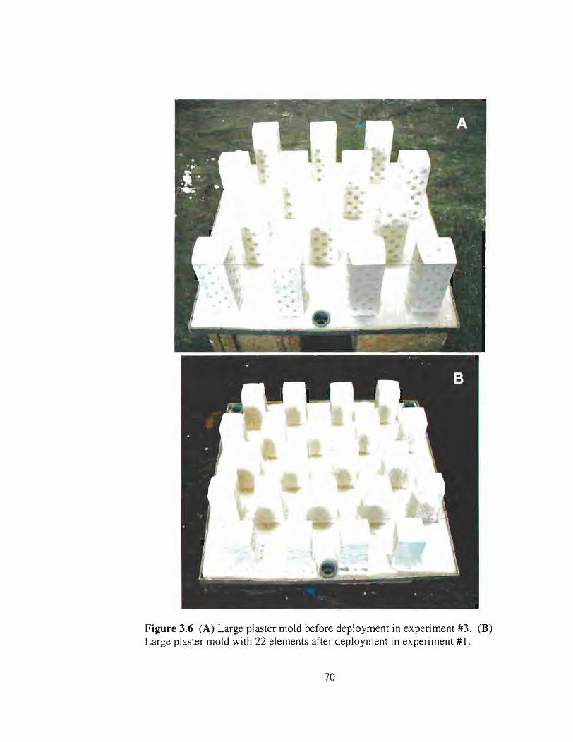
Figure 3.6 (A) Large plaster mold before deployment in experiment #3. (B)Large plaster mold with 22 elements after deployment in experiment #1.

70

Figure 3.7 Grooved plaster elements before (A) and after (B) deployment.

71

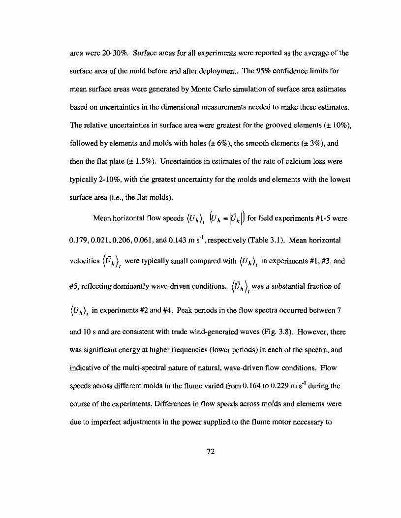
area were 20-30%. Surface areas for all experiments were reported as the average of the

surface area of the mold before and after deployment. The 95% confidence limits for

mean surface areas were generated by Monte Carlo simulation of surface area estimates

based on uncertainties in the dimensional measurements needed to make these estimates.

The relative uncertainties in surface area were greatest for the grooved elements (± 10%),

followed by elements and molds with holes (± 6%), the smooth elements (± 3%), and

then the flat plate (± 1.5%). Uncertainties in estimates of the rate of calcium loss were

typically 2-10%, with the greatest uncertainty for the molds and elements with the lowest

surface area (Le., the flat molds).

Mean horizontal flow speeds (U h), (uh'" 10hi) for field experiments #1-5 were

0.179,0.021,0.206,0.061, and 0.143 m S·l, respectively (Table 3.1). Mean horizontal

velocities (0h), were typically small compared with (Uh), in experiments #1, #3, and

#5, reflecting dominantly wave-driven conditions. (0h), was a substantial fraction of

(uh), in experiments #2 and #4. Peak periods in the flow spectra occurred between 7

and 10 s and are consistent with trade wind-generated waves (Fig. 3.8). However, there

was significant energy at higher frequencies (lower periods) in each of the spectra, and

indicative of the multi-spectral nature of natural, wave-driven flow conditions. Flow

speeds across different molds in the flume varied from 0.164 to 0.229 m S·1 during the

course of the experiments. Differences in flow speeds across molds and elements were

due to imperfect adjustments in the power supplied to the flume motor necessary to

72

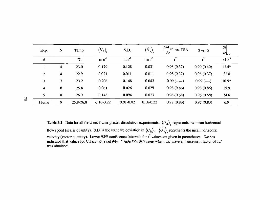
(Uh ), (0.), 8M

~Exp. N Temp. S.D. Ca vs. TSA S vs. a/::,.t a""

# DC m S·l m S·l m S-I 1 1 X 10-5

1 4 23.0 0.179 0.128 0.031 0.98 (0.37) 0.99 (0.40) 12.4*

2 4 22.9 0.021 0.011 0.011 0.98 (0.37) 0.98 (0.37) 21.8

3 3 23.2 0.206 0.148 0.042 0.99 (-----) 0.99 (----) 10.9*

4 8 25.8 0.061 0.026 0.029 0.98 (0.86) 0.98 (0.86) 15.9

5 8 26.9 0.143 0.094 0.013 0.96 (0.68) 0.96 (0.68) 14.0-.l...,

Flume 9 25.8-26.8 0.16-0.22 0.01-0.02 0.16-0.22 0.97 (0.83) 0.97 (0.83) 6.9

Table 3.1. Data for all field and flume plaster dissolution experiments. (Uh), represents the mean horizontal

flow speed (scalar quantity). S.D. is the standard deviation in (Uh)t' (0h), represents the mean horizontal

velocity (vector quantity). Lower 95% confidence intervals for 1 values are given in parentheses. Dashesindicated that values for C.I are not available. * indicates data from which the wave enhancement factor of 1.7was obtained.

0.08~--~--~--~--~--~

A0.06

\

0.04 I

0.2 0.4 0.6 0.8 1

1

B

0.80.60.40.2

~

~

~ 0.30 r---,,-~--~---~--~------,

N "en I IN 1\E 0.20 I \~ I \

~ I \ '\'iiic I \a> 0.10 I"0 I

~a> 0 L __~_~~=~ -I

c% 0

0.40 r----.---~---~--_._--~

0.30

0.20 I,, I \

I ..... / \

0.10 I \.< I '

0.2 0.4 0.6

Frequency (Hz)

0.8

c

1

Figure 3.8 Sample power spectral densities of horizontal flow speed from (A)experiment #4, (B) experiment #5, and (C) experiment #3. Mean spectra aregiven by the thick, solid black line. Gray bounds demark the 95% confidenceintervals for mean spectra. Dashed lines represent one standard deviation for allspectra.

74

maintain similar flow speeds across molds and elements of various cross-sectional area.

Once set, however, flow speeds within the flume did not vary> 1-2 cm S·I over the

course of an individual dissolution experiment (Table 3.1).

Water temperatures across all field and flume experiments ranged between 23 DC

and 27DC, leading to temperature-dependent corrections of :'05% for normalization to

25 DC (Table 3.1).

Mass transfer rates

Rates of plaster dissolution increased with surface area in all field experiments

(Fig. 3.9; Table 3.1). The correlations between the rate of calcium loss and surface area

were significant for all experiments except #3 for which there were too few data points

(N = 3) to determine the lower confidence limit. Uncertainty in estimates of SCa from the

calculation of the concentration boundary conditions according to Eqns. 3.10 & 3.11

range between 10-15% for individual elements and molds, but between 10-20% for the

flat molds. This uncertainty only affects the accuracy of estimates of SCa and not the

precision. Thus, it does not affect the comparison of results within and between

experiments. There was a significant positive correlation between SCa and a for all field

experiments (Fig. 3.10, Table 3.1), analogous to the relationship between rate of Ca loss

and surface area. There was also a significant, positive correlation between Sea and a. for

the dissolution of all molds in the flume (Fig. 3.11, Table 3.1). All values of Sea from the

flume experiments were normalized to a mean velocity of 0.192 ill S·l for the entire

75

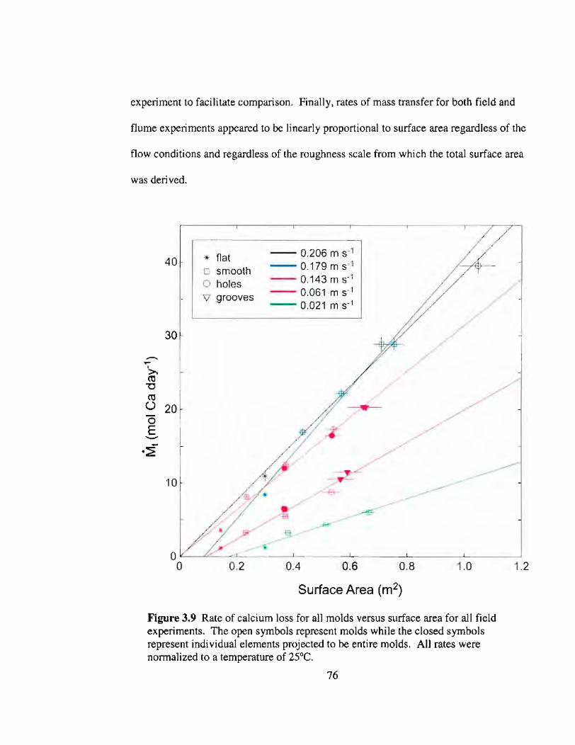
experiment to facilitate comparison. Finally, rates of mass transfer for both field and

flume experiments appeared to be linearly proportional to surface area regardless of the

flow conditions and regardless of the roughness scale from which the total surface area

was derived.

1.21.00.4 0.6 0.8

Surface Area (m2)

- 0.206 m S·1

- 0.179 m 5.1

- 0.143 m s·10.061 m s"

- 0.021 m S·1

0.2

. flato smootho holes'V grooves

O~-----L.C---"",,-..I.- ....l..- --'- ------L -----.JL-__----J

o

10

30

40

­~'>­ro"'Cro

<..> 20oE-.~

Figure 3.9 Rate of calcium loss for all molds versus surface area for all fieldexperiments. The open symbols represent molds while the closed symbolsrepresent individual elements projected to be entire molds. All rates werenormalized to a temperature of 25°C.

76

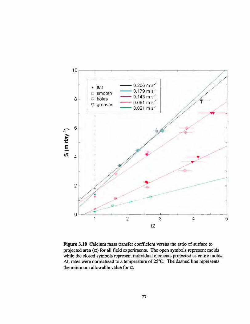
0.206 m 5-1

- 0.179 m S-l

0.143 m S-l

- 0.061 m s-1- 0.021 m S-1

flato smootho holes\l grooves

4

2

en

10 r----,---,--------r----,----r-------r----r---r---....,.....,

8

_ 6....>.CO"0

E-

QL.....-.>=:::....----l.__--L..__---I-__...I.--_------'L-_---l.__--L..__---l.-_--------i

1 2 3 4 5

Figure 3.10 Calcium mass transfer coefficient versus the ratio of surface toprojected area (a.) for all field experiments. The open symbols represent moldswhile the closed symbols represent individual elements projected as entire molds.All rates were normalized to a temperature of 25°C. The dashed line representsthe minimum allowable value for a..

77

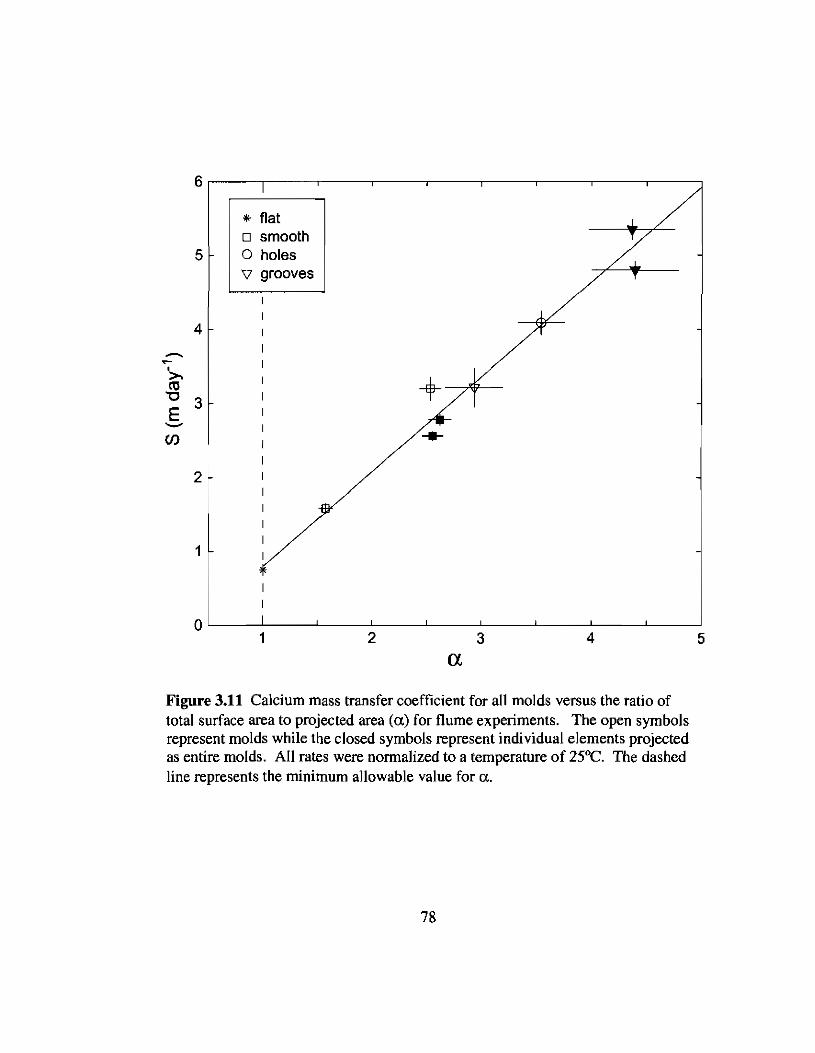
6,---,------r---,------,------,----,--------,--,-----,

* flato smooth

5 0 holes\1 grooves

4

~

~,>. +ell"0 3E-(J) ---

2

1

5432

ex

O'-----_---'---_-----L__-L.-_---'---_-----l__--'----_-----'-__.l.--_---.J

1

Figure 3.11 Calcium mass transfer coefficient for all molds versus the ratio oftotal surface area to projected area (a) for flume experiments. The open symbolsrepresent molds while the closed symbols represent individual elements projectedas entire molds. All rates were normalized to a temperature of 25°C. The dashedline represents the minimum allowable value for a.

78

Flume vs. Field experiments

The Stanton number, St, describes the rate of mass transfer a given surface will

support at a given flow speed. Therefore, in order to compare results from molds of

different surface area within an experiment, St needs to be normalized by a. As expected

mean Stla decreased with (Uh)t for all field experiments (Fig. 3.12). This relationship

is consistent with results from past flume experiments (Baird and Atkinson, 1997;

Thomas and Atkinson, 1997; Fig. 3.13). Mean Stla for the flume experiments was

significantly lower (p < 0.01) than mean Stla for field experiments by a factor of -1.7

(1.4-2.0; Fig. 3.12). Rates of dissolution from the flat plates were always proportionally

lower than all other molds for both field and flume experiments (Fig. 3.12). Thus, these

data were not included in calculation of mean Stla for each set of experiments.

Discussion

Importance ofvarying roughness scales under high Sc

Small-scale roughness features were comparable in their effect on Sea as larger­

scale roughness. This can be explained by the very high Sc characterizing the mass

transfer of dissolving gypsum. Under conditions of high Sc, the thickness of the

concentration boundary layer is much thinner than even the thickness of the viscous

sublayer where momentum transfer across the boundary layer is controlled solely by the

molecular viscosity of the fluid. An effective thin-film thickness for the concentration

79

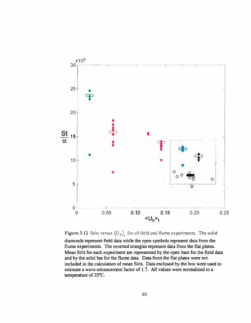
x10530 ,------------,-----,--------r-----,-----------,

25 •

20

5t 15ex

••

10

5o

0.250.200.05

0'-- .1....- .1....- .1- -'-- --'

o

Figure 3.12 St/a v r u (U,,)/ for all field and flume experiment. The olid

diamonds represent field data while the open symbols represent data from theflume experiments. The inverted triangles represent data from the flat plates.Mean Stla for each experiment are represented by the open bars for the field dataand by the solid bar for the flume data. Data from the flat plates were notincluded in the calculation of mean Stla.. Data enclosed by the box were used toestimate a wave enhancement factor of 1.7. All values were normalized to atemperature of 25OC.

80

120 ,----..-----,-----,-----,-----,------,------r---,-------,-----,

vo

100

80

..Ll')

0 Vo.....>< 60-(J) ....

v

400 00 .. 0 v

0 .. ..v .. .. o~ 0 ""

.. "..20 v vO Q;7" 0 0 0

v

0.50.40.2 0.3

Uh (m 5-1)

0.1OL-_-'-----_-L.-_...l-_---'-_---'---_----L_-'-_--'-_-----J_-----.J

o

Figure 3.13 St versus Dh for experimental reef communities based on the uptakeof phosphate (triangles) from Atkinson and Bilger (1992), uptake of ammonium(circles) from Thomas and Atkinson (1997), and the dissolution of gypsum-coatedcorals (asterisks) from Baird and Atkinson (1997). All values have beennormalized to a Sc for Ca2

+ in sea water at 25°C and 35 psu according to Eqn. 3.5.

81

boundary layer can be calculated from the total dissolution rate (M,) for a mold or

element and the surface area of the mold or element according to Fick's first law

(3.13) =

where oe is the equivalent thin·film thickness of the concentration boundary layer, and

Dl:Ca2+ is the weighted-average diffusivity of all Ca2+ species in seawater. For the field

experiments, oe varied between 30 and 150 /-lm, while oe varied between 50 and 80 /-lm

for the flume experiments. The smaller range in oe for the flume experiments reflects the

narrower range in velocities under which those experiments were conducted. In reality,

the boundary layers for turbulent flow over rough surfaces are very dynamic and

fluctuate with the formation and release of eddies adjacent to the motionless surface

(Sirovich and Karlsson 1997). Nonetheless, the thin·film thickness estimated for these

experiments suggests that the concentration boundary layer is thin enough to make a

chemically or biologically active surface area resulting from features larger than -1 mm

in scale available for mass transfer.

Although the above reasoning can explain why small·scale roughness features are

important to rates of calcium and nutrient mass transfer, the apparently linear

relationships between observed mass transfer rates and total surface area under all flow

conditions is still surprising. Past studies have demonstrated that rates of plaster

dissolution were proportional to the surface area of the plaster form (Porter et al. 2000;

Thompson and Glenn 1994). However, these relationships were either complex and/or

82

non-linear even though the plaster objects used in these experiments were geometrically

simpler than those used here (i.e., single spheres and cubes). Results presented here may

be partly due to the consistent and symmetric manner in which all the molds were

constructed. Providing this consistency in the experimental design allowed for a direct

comparison of mass transfer rates for similar forms under varying flow conditions, as

well as for varying forms under the same flow conditions. However, the relationship

between nutrient mass transfer rates and surface area for natural reef organisms and

communities with extrusive morphologies may be more complicated. For example,

scales of roughness added to the plaster elements and molds used in these experiments

were intrusive (holes and grooves) rather than extrusive (branches and nubs). The results

of these experiments are meant only to imply that rates of mass transfer are correlated

with available surface area, regardless of the scale from which this surface area is derived

over the roughness scales considered (0.001 - 0.01 m).

Independence ofindividual element dissolution rates

Rates of mass transfer for the individual elements were very much comparable

with those of the larger molds in both the flume and field experiments (Figs. 3.10 &

3.11). This indicates that elements within a mold interacted independently with the flow

in terms of their mass transfer rates. It is possible that the distribution of elements on the

smaller molds, combined with the orientation of the mold with the predominant direction

of flow, ensured that all elements were receiving the maximum amount of exposure to the

flow (Fig 3.1A). However, results from experiments #1 and #2 gave rates of plaster

83

dissolution which were linearly proportional to surface area, even though the number and

density of elements were higher than in experiments #3-5. The elements on one mold in

experiments #1 and #2 were only separated by distances of roughly 1/2 the element width

and 1/3 the element height (Fig. 3.6B). This result suggests that individual reef

organisms may not be substantially affected by the physical presence of adjacent

organisms in terms of their mass transfer characteristics as long as those adjacent

organisms are of similar size and separation. The feedback of the roughness of reef

organisms on rates of mass transfer for individual organisms may occur at the community

scale, i.e., spatial scales which are much larger than that of the individual organisms.

Flume vs. Field experiments

The degree to which turbulence is developed within the ambient flow may have

an important effect on the observed mass transfer characteristics in the flume and field.

Past flume experiments have shown that St decreases more dramatically with U h for Uh <

0.05 m S·I than for Uh > 0.10 m S'I (Fig. 3.13). The experimental relationship between St

and Uh in Fig. 3.13 is equivalent to an experimental relationship between St and Reynolds

number, Re '" UhUV, since the length scales, L, in each of these experiments were

comparable. St 0<: Re'O.5 for a flat plate under laminar flow conditions, while under fully

turbulent flow St '" Re'O.l (Kays and Crawford 1993). Consequently, the relationship

shown in Fig. 3.13 may indicate that these communities underwent a transition to

turbulence for Uh, between 0.05 and 0.10 m S·I. However, the large scatter in St at flow

speeds < 0.05 m S'l could also be the result of small uncertainties in estimates of Uh given

84

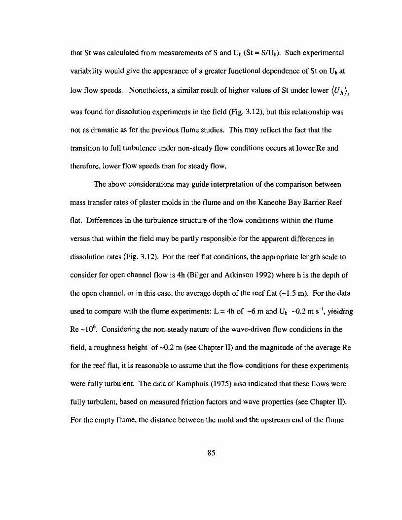
that St was calculated from measurements of Sand Uh (St '" SlUh). Such experimental

variability would give the appearance of a greater functional dependence of 5t on Uh at

low flow speeds. Nonetheless, a similar result of higher values of 5t under lower (Uh) t

was found for dissolution experiments in the field (Fig. 3.12), but this relationship was

not as dramatic as for the previous flume studies. This may reflect the fact that the

transition to full turbulence under non-steady flow conditions occurs at lower Re and

therefore, lower flow speeds than for steady flow.

The above considerations may guide interpretation of the comparison between

mass transfer rates of plaster molds in the flume and on the Kaneohe Bay Barrier Reef

flat. Differences in the turbulence structure of the flow conditions within the flume

versus that within the field may be partly responsible for the apparent differences in

dissolution rates (Fig. 3.12). For the reef flat conditions, the appropriate length scale to

consider for open channel flow is 4h (Bilger and Atkinson 1992) where h is the depth of

the open channel, or in this case, the average depth of the reef flat (-1.5 m). For the data

used to compare with the tlume experiments: L = 4h of -6 m and Uh -0.2 m S·l, yielding

Re _106• Considering the non-steady nature of the wave-driven flow conditions in the

field, a roughness height of -0.2 m (see Chapter II) and the magnitude of the average Re

for the reef flat, it is reasonable to assume that the flow conditions for these experiments

were fully turbulent. The data of Kamphuis (1975) also indicated that these flows were

fully turbulent, based on measured friction factors and wave properties (see Chapter II).

For the empty flume, the distance between the mold and the upstream end of the flume

85

was -7.5 m and Uh was 0.12-0.18 m s-', yielding values ofRe of between 106 and

1.5x 106 (vsw =0.ge-6). For a flat plate whose edge begins under laminar flow

conditions, Re of these magnitudes would represent a region of transition to turbulence

and not fully turbulent flow (Kundu 1990). However, a number of points must be

considered. First, the presence of walls along the sides of the flume would suggest that

transition to turbulence for the flume would occur at lower critical Re than for a flat plate.

Second, the surfaces of the flume have minor abrasions which prevent it from being

considered a perfectly smooth surface. Third, before water flowed down the open

channel of the flume used in these experiments, it passed through a 1800 tum which

created exit vortices that were strong enough to create local reversals in flow direction

near the walls within -0.5 m of the exit. Consequently, flow within the flume began in a

fully turbulent state. Fourth, the turbulent nature of flow within the flume was later

visually confirmed with the injection of dye into the flume under the above flow speeds,

followed by dispersion of the dye patch. Finally, it is possible that the local turbulence

generated by the non-streamlined, rectilinear geometries of the molds and elements

themselves are more important in defining their mass transfer characteristics than are

turbulence levels in the ambient flow environment.

The exact relationship between rates of mass transfer to a given surface and the

ambient turbulence field is beyond the scope of the present study. Furthermore, it would

be unwise to interpret differences between mass transfer rates observed in the flume used

here and in the field as being representative of differences between mass transfer rates to

rough surfaces under steady and non-steady flow conditions in general. However, results

86

presented here do indicate a significant enhancement of mass transfer rates for surfaces of

similar shape and roughness scale under the oscillatory flows measured in the field and

the steady flows created by the flume. The exact mechanisms responsible for this

enhancement have yet to be determined. Given the relationship between St and

(Uh)1 determined under a range of flow speeds in both the field (Fig. 3.12) and flume

(Fig. 3.13), it is unlikely that the factor of 1.7 enhancement in rates of mass transfer

changes much for 0.05 < (Uh)1 < 0.5 m S·I. Uncertainties in the exact dependence of St

on (Uh)1 for (Uh)1 < 0.05 m S'I make quantifying any wave-driven enhancement within

this domain difficult to bound. Furthermore, the conditions for which (Uh) t < 0.05

m S'l in the field are likely to result from a combination of steady and oscillatory flow.

Thus, an enhancement factor describing differences in mass transfer rates between

oscillatory flow and steady flow may not even be meaningful for(Uh)t < 0.05 m S'I.

Estimates ofS for a Kaneohe Bay Barrier Reefflat community

The primary purpose of these experiments was to provide independent estimates

of nutrient mass transfer rates to compare with the results from Chapter III. Communities

used in flume mass transfer experiments by Atkinson and Bilger (1992), Thomas and

Atkinson (1997), and Baird and Atkinson (1997) gave St of 20x 10,5 to 30x 10'5 at flow

speeds around 0.20 m S'I when normalized to a Sc for Ca2+ at 25°C and 35 psu (Fig.

3.13). These values of St are equivalent to Sea between 3.5-5.2 m day'l. The data

87

presented here would indicate that these experimental communities had values of a

between 3.5 and 4.5 (Fig. 3.11). The organisms used in these experimental communities

were of roughly the same size as those covering most of the Kaneohe Bay Barrier Reef

flat community studied earlier (-0.2 m; field observations). Consequently, it is likely that

a for that reef flat community lies between 3 and 5. Mean flow speeds across the reef

flat community are 0.1-0.2 m s'!, given average wave heights outside Kaneohe Bay

(mean Hsig = 2.0 m; see Chapter II). The above range in a and (Uh) t indicate that the

average S for this reef flat community should be somewhere between 5-9 m day'! for

dissolved phosphate and 8-15 m day'! for nitrate and ammonium. Uncertainty from both

the regression shown in Fig. 3.11 and calculation of the boundary conditions for

dissolved calcium across the concentration boundary layer would introduce an additional

uncertainty of about ±15% in these estimates. Therefore, these communities would be

expected to have an average S of 7 ± 3 m day'l for dissolved phosphate and 12 ± 5 m

day'l for nitrate and ammonium.

88

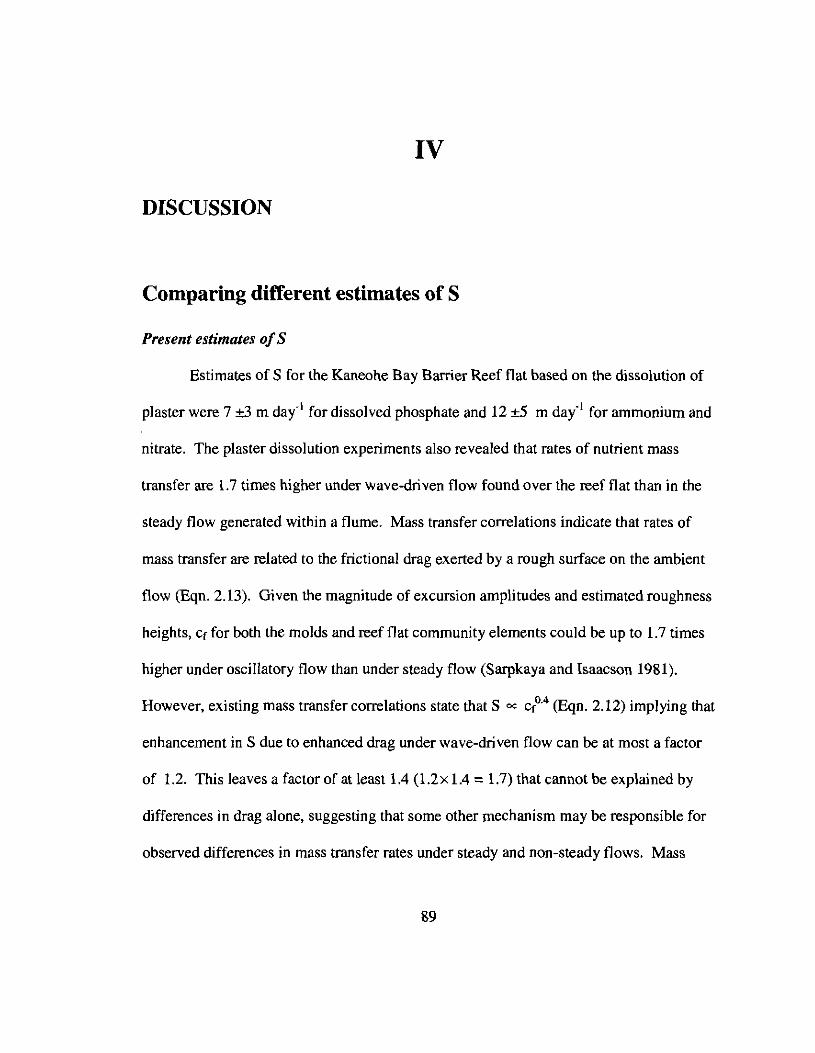
IV

DISCUSSION

Comparing different estimates of S

Present estimates ofS

Estimates of S for the Kaneohe Bay Barrier Reef flat based on the dissolution of

plaster were 7 ±3 m day·1 for dissolved phosphate and 12 ±5 m dai1 for ammonium and

nitrate. The plaster dissolution experiments also revealed that rates of nutrient mass

transfer are 1.7 times higher under wave-driven flow found over the reef flat than in the

steady flow generated within a flume. Mass transfer correlations indicate that rates of

mass transfer are related to the frictional drag exerted by a rough surface on the ambient

flow (Eqn. 2.13). Given the magnitude of excursion amplitudes and estimated roughness

heights, Cf for both the molds and reef flat community elements could be up to 1.7 times

higher under oscillatory flow than under steady flow (Sarpkaya and Isaacson 1981).

However, existing mass transfer correlations state that S oc CfO.4 (Eqn. 2.12) implying that

enhancement in S due to enhanced drag under wave-driven flow can be at most a factor

of 1.2. This leaves a factor of at least 1.4 (1.2x 1.4 = 1.7) that cannot be explained by

differences in drag alone, suggesting that some other mechanism may be responsible for

observed differences in mass transfer rates under steady and non-steady flows. Mass

89

transfer correlations for rough surfaces were developed in the absence of form drag.

Form drag results from the separation of flow streamlines from surfaces of an object,

leading to the formation of turbulent eddies. Relationships between mass transfer rates

and drag may be different when form drag is the dominant source of bottom friction, such

as over coral reef communities. Nonetheless, Atkinson et al. showed that existing mass

transfer correlations to predict rates of nutrient uptake for experimental communities

which are characterized by high drag and roughness height (Rek '" 103_105), and high Sc

(500-1500)(Baird and Atkinson 1997; Thomas and Atkinson 1997). Results from the

plaster dissolution experiments indicate that rates of mass transfer were proportional to

surface area. Frictional drag exerted on marine macroalgae increase with the surface area

of the algae (Gaylord et al. 1994). These results indicate that a correlation between form

drag and mass transfer rates should still exist: in other words, larger organisms will have

greater surface area than smaller organisms and should thus exhibit higher rates of mass

transfer and higher drag.

Using an empirical mass transfer relationship based on the experimental data of

Atkinson et al. and in situ estimates of Uh, Cr, and k for the reef flat community gave

estimates of S (5.8 ±O.8 m day" for dissolved phosphate and 9.7 :1:1.3 m day·l for

ammonium and nitrate) which were remarkably close to estimates based upon the

dissolution of plaster molds (± 20%). Values of Uh, cr, and k for the reef flat community

were similar to those used in prior flume experiments. Therefore. values of Rek, and Sc

between experimental flume communities and the Kaneohe Bay Barrier Reef flat

community were also similar in scale. Consequently, application of the empirical mass

90

transfer relationship derived from experimental reef communities in a flume to that of the

reef flat did not entail much of an extrapolation. The only major difference between the

two communities was that flow in the flume was steady while flow on the reef flat is

predominantly oscillatory. Therefore, estimates of S for the reef flat community based on

the empirical mass transfer correlation should be scaled up by a factor of around 1.4

based on previous consideration of wave enhancement. Applying this scaling gives

values for S equal to 9.2 ±2.1 m day"' for dissolved phosphate and 15.3 ±3.4 m day"1 for

ammonium and nitrate. These revised estimates are slightly higher than those based

solely on the dissolution of plaster molds and may reflect slightly higher values of a, Cr,

and k for the Kaneohe Bay Barrier Reef flat community than the experimental

communities used by Atkinson et al.

Past estimates ofSnet

The best mass transfer estimate of S for the maximum rate of gross phosphate

uptake by the Kaneohe Bay Barrier Reef community is 9.2 ±2.1 m day"l. This is

comparable with a first-order rate constant of 9 m day"l for net phosphate uptake (Snet)

estimated by Atkinson (l987a). Atkinson (1987a) made his phosphate measurements

following the method of flow respirometry using both drogues and dye patches as

Lagrangian tracers. His calculation of Snet was based on a mean phosphate concentration

gradient across the Kaneohe Bay Barrier Reef flat calculated from monthly transects

taken over an entire year (Fig. 4.1), and a cross-reef transport rate (Q') of 0.06 m3 S·l m'l

derived from the movement of drogues and dye patches

91

(4.1) Snet =0Q'

where 0is the spatial phosphate concentration decay constant detennined from log-

transformation of phosphate concentration versus distance (1.73 x 10-3 m-l ; Fig. 4.1).

0.15-,-----------------~ -2

• -3

0.10.......• c..

,. Q- ,. -:2 • cE -4-c.. • ,.Q • ,.

0.05 • ,. ,.

• -5• • •

• •-------------------.---• ••o-'---,--------,-----,----,--------,-----.---,------J

o 500 1000Distance (m)

1500

Figure 4.1 Dissolved inorganic phosphate concentrations across the Kaneohe BayBarrier Reef flat (Atkinson, 1987a). Closed circles represent the annual mean of monthlymeasurements taken within 50 m of the plotted position (standard error < O.0121-\M).The triangles represent log-transformed DIP concentrations. The regression slope ofIn(DIP) versus distance is -1.73x 10-3 mol. This value was used to estimate a first-ordernet phosphate uptake rate constant of 9 m day"l. The dashed line indicates the limits ofanalytical detectability. Points lying below this line were not included in the regression ..

92

The estimate of Q' made by Atkinson (1987a) was consistent with the results of

Bathen (1968) who measured Q' using both drogues and current meters. However, it is

possible that both Bathen (1968) and Atkinson (1987a) overestimated Q'. If so, this

would result in an overestimation of Sne' (Eqn. 4.1). The use of drogues in regions where

wave-driven velocities are much higher than mean currents is suspect due to the transfer

of momentum from the waves to the drogue, causing it to bias mean current speeds in the

direction of wave propagation. Dye patches would not be susceptible to such momentum

artifacts; however, the constant dispersion and renewal of the dye patch, which are

necessary over the course of a flow respirometry experiment, make them susceptible to

error as well. Furthermore, both of these authors relied on triangulation for estimating

drogue and dye patch positions. Precision in these measurements depends on the

alignment and position of the markers used as well as the total distance traversed. It is

also unlikely that Bathen (1968) would have had current meters precise enough at the

time to measure the relatively small cross-reef currents on the Kaneohe Bay Barrier Reef.

In fact, re-evaluation of Bathen's data suggest that a cross-reef transport of 0.06

m3S-I m- I represented an upper limit for current meter measurements made on the reef

flat.

Mean cross-reef velocities measured in this study were between 0.01 and 0.04 m

S-I, and even lower if averaged over a 2-hour interval. Using a depth of 1.4 m averaged

over the study area and over the four tidal cycles using all the data gives a cross-reef

transport of around 0.03 m3S-l m-I

• In addition, estimates of cross-reef currents from a

93

field class reported cross-reef velocities of 0.01-0.03 m S·I over an entire tidal cycle (M.

Atkinson, unpub!. data). Given the depths reported during that study, these velocities

would also correspond to an average Q' of 0.03 m3S·I m· l

•

Waves propagating across the reef could serve as a source of mass transport due

to non-linear effects (Dean and Dalrymple 1991). The range in rms-wave heights

presented earlier would yield depth-averaged flow speeds of 0.01-0.03 m S·I (Dean and

Dalrymple 1991). However, it is uncertain how cross-reef pressure gradients would

oppose this transport given the attenuation in wave height and associated elevation in

water level necessary to balance the decreasing radiation stress resulting from the

attenuation of waves across reef (Longuet-Higgins and Stewart 1964). The very small

cross-reef currents occurring on the Kaneohe Bay Barrier Reef flat are likely the result of

its 2-km width, much wider than for most reefs (Symonds et al. 1995; Wiens 1962). If a

cross-reef Q' of 0.03 m3S·I m·1 were accepted as being more typical, then estimates of S

made by (Atkinson 1987a) would be reduced by half to 4.5 m day'l. However, Atkinson

(1987a) could have acquired his data under higher wave conditions which resulted in

greater cross-reef currents. The above arguments simply identify the uncertainty in

estimates of Snet that can result from uncertainty in Q'.

The true time-averaged value of Snet probably lies somewhere between 4.5 and 9

m day'l since estimates of Q' made here were made over an entire tidal cycle while

estimates of Q' made by Atkinson (l987a) were made only during rising tides. The

important point is that estimated rates of net phosphate uptake are comparable to, but do

not exceed, predicted rates of maximum gross phosphate uptake.

94

S for other reef communities

Direct measurements of first-order uptake rate coefficients of phosphate,

ammonium, and nitrate rates in low-energy reef environments, however, have yielded

values which are only marginally smaller than nutrient mass transfer coefficients made

here. Steven and Atkinson (in press) measured the gross uptake of phosphate and

ammonium in isolated microatolls within the lagoon of One Tree Island, GBR and

estimated rate coefficients of 5.8 m daiJ for phosphate and 7.5 m daiJ for ammonium.

However, flow velocities were not measured in that study. Atkinson et aI. (2001)

measured gross uptake rate coefficients of 7.4,7.5, and 4.4 m day- J for phosphate,

ammonium, and nitrate respectively in the Biosphere 2 reef mesocosm where water

velocities were between 0.05-0.15 m s-J. These studies would suggest that I may be

underestimating nutrient mass transfer coefficients for the Kaneohe Bay Barrier Reef flat.

However, the physical biological details of nutrient removal processes in these studies

were not well characterized, only the rate of decay in nutrient concentrations.

Additionally, part of the discrepancy between direct measurements and predictions of

nutrient mass transfer coefficients made here may be explained by higher values of St at

low flow speeds, even under non-steady flow conditions. This characteristic modulates

changes in S with <Uh>, such that they do not decrease proportionately (Fig. 3.12)

Furthermore, uncertainty in both estimates and measurements of S of 1-3 m dal may be

typical and cannot be neglected when comparing nutrient mass transfer coefficients

between different reef environments.

95

Nutrient uptake and net primary production

Estimates of S for net and maximum gross phosphate uptake rates reported here

are comparable in magnitude, indicating that phosphate uptake by the Kaneohe Bay

Barrier Reef flat is mass transfer limited. A substantial fraction (>50%) of the dissolved

phosphate fixed on the reef flat is exported as organic phosphorus compounds rather than

excreted back into the water column as inorganic phosphate, consistent with observations

made by Atkinson (1981b). This description of phosphate metabolism in coral reef

communities is much different from that of organic carbon metabolism. Nearly all of the

organic carbon produced by most coral reef communities are consumed via respiration

and only small fraction of organic carbon, typically less than an order of magnitude, is

either imported or exported (Crossland et al. 1991; Kinsey 1985). This indicates that a

greater fraction of the phosphate taken up by reef communities remains in organic matter

than does fixed carbon. The idea of nutrient uptake regulating net primary production

can be pursued further by scaling rates of nutrient uptake by the C:N:P ratios of benthic

reef autotrophs to compare them with rates of photosynthetic production.

Maximum phosphate and nitrogen ]luxes

Two transects taken across the study area in August and September of 2000 of the

Kaneohe Bay Barrier Reef flat yielded dissolved phosphate concentrations of 0.09 ± 0.01

IlM. These concentrations are consistent with the measurements of Atkinson (1987a) for

96

that area of the reef flat (Fig. 4.1), as well as measurements from transects made across

that area in the summer of 1995 (0.08-0.10 11M; M. Atkinson et a!., unpubl. data).

Furthermore, these concentrations are comparable to concentrations measured outside

Kaneohe Bay between the fall of 1998 and the summer of 2001 (Kinzie III et a1. 2001)

and in earlier studies (Smith et a!. 1981), as well as concentrations measured in waters

-10 km northwest of Oahu over the past 14 years (Fig. 4.2A). Based upon an estimated S

of 9.2 m dai l, maximum rates of dissolved phosphate uptake should be around 0.8 mmol

Pm·2dai ' (!Pm.x) under typical wave conditions according to

(4.2) Jmax = Sj Cj

where Cj is the concentration of nutrient i in the water. These rates are considered

maximal because they assume that nutrient concentrations at the surfaces of reef

autotrophs are negligible (see Chapter II). The same data sets indicate that dissolved

inorganic nitrogen (DIN - nitrate + ammonium) concentrations from the same waters

vary within the range of 0.1-0.3 11M. These concentrations translate into maximum rates

of DIN uptake (JNmax) of around 3.1 mmol N m,2 day'l (Fig. 4.2B).

Estimates ofnet and gross primary production

Atkinson and Smith (1983) measured the molar C:N:P ratio of twenty species of

benthic algae found on Hawaiian reefs and obtained an average ratio of 640:34: 1. Chun­

Smith (1994) obtained a similar average C:N:P ratio (790:31:1) for benthic macrophytes

collected from the reef flat near Kapapa Island. These data indicate that Hawaiian reef

97

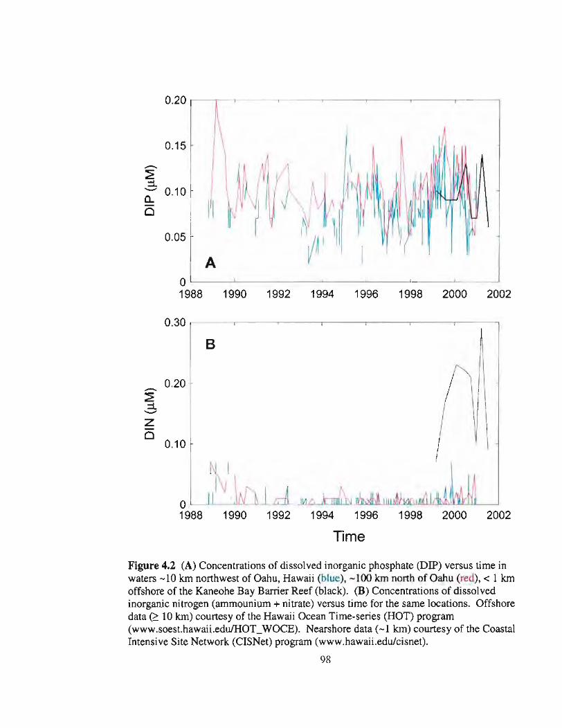
A

0.20 .------.-----,----,-------r----.----.-----,--------,

0.05

0.15

--~::l~ 0.10

o II

1998 2000 20021996199419921990o"------__--'--__-'-__----'-__--1. -'------__---L-__--'

1988

0.30 .----------,----,-------r----.-----,------,-----,

B

1998 2000 20021996199419921990O'----'-'-_...J.U..:lL........Ll'-'--.L.I-..J"'--.J.LLL...>.....l.Joj-.I..LW~...ILJLIo<Jl.LUl....l..l.l..l..Ll.I.....II!>!L.l..l.lIctl..Lll_..lUU.JU-I.lUL..U.Il_--'

1988

0.20

0.10

--~::l--Zo

Time

Figure 4.2 (A) Concentrations of dissolved inorganic phosphate (DIP) versus time inwaters -10 km northwest of Oahu, Hawaii (blue), -100 km north of Oahu (red), < 1 kmoffshore of the Kaneohe Bay Barrier Reef (black). (B) Concentrations of dissolvedinorganic nitrogen (ammounium + nitrate) versus time for the same locations. Offshoredata (2: 10 km) courtesy of the Hawaii Ocean Time-series (HOT) program(www.soest.hawaii.eduIHOT_WOCE). Nearshore data (-1 km) courtesy of the CoastalIntensive Site Network (CISNet) program (www.hawaii.edu/cisnet).

98

autotrophs have C:N ratios of around 22 on average. Using an average C:P ratio of 640: 1

for benthic Hawaiian autotrophs, Atkinson (1981a) showed that his estimate for the

average rate of net phosphate uptake (-0.5 mmol P m·2day"l) could be scaled to a net

community production rate of 300 mmol C m,2 day' I estimated by Webb (1977)

following an ecological principle put forth by Odum (1971). This principle states that the

amount of net phosphate taken up by a community should balance the net growth of, or

export of organic carbon from, that community if the C:P ratio of the average organic

material is known. An analog of this principle would be that rates of net primary

production (NPP) within a community is equivalent to the gross rate of nutrient uptake

scaled by the average C:N:P ratio of autotrophic biomass. Scaling a JPmax of 0.8 mmol P

m,2 day' I for the Kaneohe Bay Barrier Reef flat community in this way yields NPP equal

to 510 mmol C m,2 day,l if a C:P ratio of 640: 1 is used (Atkinson 1981 a; Atkinson and

Smith 1983) and 630 mmol C m,2 day"I if a C:P ratio of 790: 1 is used (Chun-Smith

1994).

Webb (1977) estimated rates of gross community production (OPP) of 1300

mmol C m,2 day,l for the same area of the reef flat studied here, based on flow

respirometry data. Changes in dissolved oxygen concentrations across that study area, as

well as changes in dissolved oxygen concentration with time at a single point within the

study area, measured by M. Atkinson et aJ. (unpubJ. data) yield a similar estimate of 1500

mmol C m,2 dal for OPP. These values are close to the rates of around 1700 mmol C

m,2 day'l for areas of 100% hard-bottom cover by algae and/or coral (i.e., not sand)

demonstrated by Kinsey (1985) for many reefs around the world. It is very likely that the

99

Kaneohe Bay Barrier Reef flat is close to this model of standard reef metabolism. As

stated earlier, the study area had very little sand cover (Fig. 2.3). In addition, descriptions

of the bottom community made here are consistent with prior descriptions made by an

oceanography field class (unpub!. data) and later by Chun-Smith (1994) indicating that

the metabolism of the bottom community has remained largely unchanged. Comparing

the above data on GPP with estimates of NPP indicates that roughly half of the organic

carbon produced via photosynthesis by reef autotrophs is being either respired or

exported. Furthermore, recent studies in a large coral reef mesocosm (Biosphere II, 850

m2) indicate that rates of community respiration in the light are twice as high as rates of

respiration in the dark (Langdon et a!. In press). Historically, such independent

measurements of light respiration were unable to be made in the field. Therefore, rates of

dark respiration were assumed to be representative of the rate of community respiration

over an entire diurnal cycle, even though past investigators recognized the potential error

in this assumption. The Biosphere 2 results indicate that historical estimates of gross

primary production are actually 50% higher than previously reported implying that NPP

across the Kaneohe Bay Barrier Reef flat community could be roughly one-third GPP.

Rates of NPP estimated by scaling rates of maximum DIN uptake are lower than

estimates based on maximum dissolve phosphate uptake (30 to 115 mmol C m-2 day"l).

However, the demand for fixed nitrogen by reef communities could be subsidized by

nitrogen fixation (Smith, 1984; Atkinson, 1992). Unfortunately, estimates of nitrogen

fixation rates at the community scale can not be extrapolated from prior studies

(Carpenter et al. 1991; Wiebe et al. 1975; Wilkinson et al. 1984; Williams and Carpenter

100

1998), making it difficult to assess how much benthic reef autotrophs depend on nitrogen

fixation as a source of fixed nitrogen.

The preceding discussion presents a biogeochemical model of shallow-water coral

reef communities which, living in an environment of high incident light and low ambient

nutrient concentrations, can produce enough organic carbon to grow tissue of very high

C:N:P in comparison with planktonic organic matter, and still have enough excess

organic carbon to maintain high enzyme affinities and thus take up nutrients at near-mass

transfer limits (Atkinson 1987b; Atkinson and Bilger 1992; Atkinson et al. 1994; Lamed

and Atkinson 1997; Thomas and Atkinson 1997), and 2) fuel other energetically costly

processes such as nitrogen fixation (Carpenter et al. 1991; Wiebe et al. 1975; Wilkinson

et al. 1984; Williams and Carpenter 1998).

Spatial zonation in reef metabolism

The maximum rate of nutrient uptake is the product of the mass transfer

coefficient and the concentration of the nutrient in the water (Eqn. 4.2), and Si is

primarily a function of the friction coefficient (Cf) and horizontal flow speed (U)

(4.3)

Spatial zonation in JmaXo and therefore NPP, will follow the spatial zonation in these

parameters.

101

Fore reef

Wave energy impinging upon the Kaneohe Bay Barrier Reef, and the rest of the

windward coast of Oahu comes from 1) trade wind-generated waves out of the east to

northeast, and 2) winter swells from the north to northwest (Fig. 4.3). Although direct

measurements of wave characteristics on the fore reef of the Kaneohe Bay Barrier Reef

were not made during the course of this study, we can simulate the spatial gradients in

near-bottom velocities along the fore reef with a numerical wave transformation model:

SWAN (Simulating WAves Nearshore; Delft University, Netherlands). SWAN was used

to transform the average nearshore directional wave spectrum (Fig. 4.3) as it propagates

onto the fore reef of the Kaneohe Bay Barrier Reef. Briefly, SWAN is a third-generation

wave model based on a simple energy action equation allowing for various sources and

sinks which include wind stress, white-capping, bottom friction, shoaling and refraction,

breaking, and various wave-wave interactions. For this simulation, the bottom friction

coefficient was assumed to be 0.2 everywhere and the effects of local wind stresses were

ignored. This is similar to a Cf of 0.1 estimated for the fore reef of Ala Moana Reef on

the south shore of Oahu, Hawaii (Gerritsen 1981). Unfortunately, the model will not

accurately estimate the height of waves inside of the breaking zone due to its inability to

readjust the depth-limited wave height parameter (y) to much lower values representative

of the inner surf zone (Raubenheimer et aI. 1996). Consequently, simulation of wave

heights are valid only for the fore reef. Model simulations do indicate that wave trains

with H'ig of 2.0 m, or Hon, of 1.5 m, remain relatively constant in amplitude as they move

from deep water onto the fore reef (Fig. 4.4). These results appear to be consistent with

102

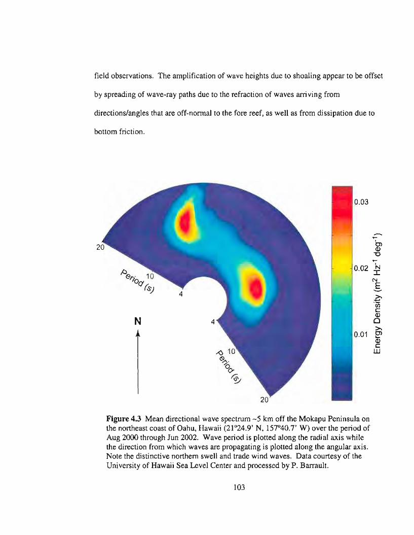
field observations. The amplification of wave heights due to shoaling appear to be offset

by spreading of wave-ray paths due to the refraction of waves arriving from

directions/angles that are off-normal to the fore reef, as well as from dissipation due to

bottom friction.

0.03

­.....IC)Q)"0

.....0.02 ~

N

E-~·wc:Q)

o>-

0.01 ~Q)c:W

Figure 4.3 Mean directional wave spectrum -5 km off the Mokapu Peninsula onthe northeast coast of Oahu, Hawaii (21°24.9' N, 157°40.7' W) over the period ofAug 2000 through Jun 2002. Wave period is plotted along the radial axis whilethe direction from which waves are propagating is plotted along the angular axis.Note the distinctive northern swell and trade wind waves. Data courtesy of theUniversity of Hawaii Sea Level Center and processed by P. Barrault.

103

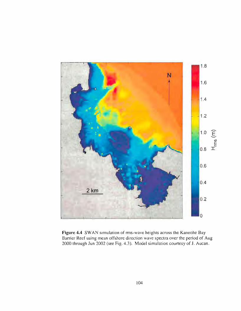
2km

1.8

1.6

1.4

1.2

..-1.0 E--en

E....0.8 I

Figure 4.4 SWAN simulation of nns-wave heights across the Kaneohe BayBarrier Reef using mean offshore direction wave spectra over the period of Aug2000 through Jun 2002 (see Fig. 4.3). Model simulation courtesy of J. Aucan.

104

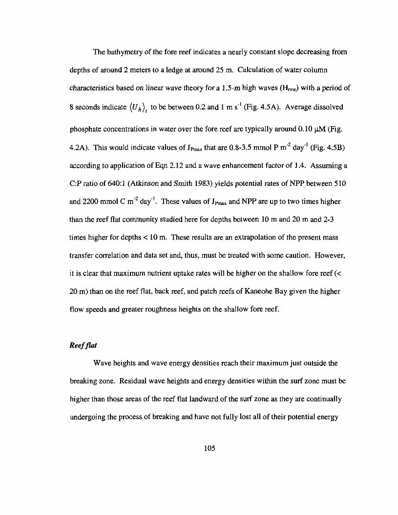
The bathymetry of the fore reef indicates a nearly constant slope decreasing from

depths of around 2 meters to a ledge at around 25 m. Calculation of water column

characteristics based on linear wave theory for a 1.5-m high waves (Hnns) with a period of

8 seconds indicate (Uh) t to be between 0.2 and I m sol (Fig. 4.5A). Average dissolved

phosphate concentrations in water over the fore reef are typically around 0.10 lJM (Fig.

4.2A). This would indicate values of JPmax that are 0.8-3.5 mmol P mo2 day"! (Fig.4.5B)

according to application ofEqn 2.12 and a wave enhancement factor of 1.4. Assuming a

C:P ratio of 640:1 (Atkinson and Smith 1983) yields potential rates of NPP between 510

and 2200 mmol C mo2

day'!. These values of JPmax and NPP are up to two times higher

than the reef flat community studied here for depths between 10 m and 20 m and 2-3

times higher for depths < 10 m. These results are an extrapolation of the present mass

transfer correlation and data set and. thus. must be treated with some caution. However,

it is clear that maximum nutrient uptake rates will be higher on the shallow fore reef «

20 m) than on the reef flat, back reef, and patch reefs of Kaneohe Bay given the higher

flow speeds and greater roughness heights on the shallow fore reef.

Reefflat

Wave heights and wave energy densities reach their maximum just outside the

breaking zone. Residual wave heights and energy densities within the surf zone must be

higher than those areas of the reef flat landward of the surf zone as they are continually

undergoing the process of breaking and have not fully lost all of their potential energy

105

1.0 ,-------,,-----,----r-----,---.-----.------,-------,-----,---,

0.8

~

~

(n 0.6E~

A.c 0.4

::>v

0.2

A

O'-------'-------'-----'-----'------"'-------'-------'-----'--------L---'o 2 4 6 8 10 12 14 16 18 20

4,------,----.-----.-----,----.---r--,-----,------,---,

B

2 4 6 8 10 12

Depth (m)

14 16 18 20

Figure 4.5 Simulation of (A) average near-bottom horizontal flow speeds and(B) maximum phosphate uptake rate resulting from the propagation of a 1.S-mwave of 8-s period over the fore reef of the Kaneohe Bay Barrier Reef, based onsimulations from a numerical wave model (SWAN). Depths less than 2 m werenot considered due to the initiation of wave breaking.

106

according to the depth-limitation of wave amplitude. Furthermore, superimposed on

these residual waves are the kinetic energy of bores created in the breaking process which

have converted the potential energy of the excess wave height into kinetic energy. Flow

speeds should reach their greatest values within the surf zone. However, I am unable to

properly characterize flow conditions within the surf zone and thus unable to characterize

JPmax and NPP within the surf zone.

Past the landward extent of the surf zone, residual waves continue to propagate

and attenuate in height due primarily to frictional dissipation along the bottom (Chapter

II). These 6-10 s period waves die out before leaving the back-reef area of the reef flat

where only short period « 4 s) wind chop remains (field observations). This general

process of wave transformation over coral reefs has been amply theorized and

documented (Gourlay 1994; Hardy and Young 1996; Heam and Parker 1988; Heam

1999; Hearn et al. 2001; Lugo-Fernandez 1998a, 1998b; Massel and Gourlay 2000; Munk

and Sargent 1954; Nelson 1996; Symonds et al. 1995; Tait 1972; Young 1989).

There was no significant variation in Cf over the studied area of the Kaneohe Bay

Barrier Reef flat. This value of Cf (0.22) is applicable to a zone of -500 m from where

the bottom type can be completely described as rough hard-bottom colonized mostly turf

and macroalgae and some scattered coral heads (see Chapter II). J Pmax within the zone

-500 m from the reef crest are estimated to range between 0.4 and 1.0 mmol P m-2 dati

based on the observed range in (Uh) t of 0.1-0.2 m S·l and concentrations (0.06-0.10 J.lM;

Fig. 4.1). Assuming a C:P ratio of 640:1 (Atkinson and Smith 1983), this translates into

107

NPP between 260 to 640 mmol C m'2 dal with the values decreasing with distance from

the surf zone owing to wave attenuation, A higher C:P ratio of 790: 1 would imply NPP

between 320 and 790 mmol C m'2 dal (Chun-Smith 1994),

The increasing coverage of sand towards the back of the reef flat could result in

decreasing bottom roughness on average (Fig. 2.3). However, the combination of sand

ripples and decreasing wave orbital amplitudes (Arms) would suggest that Cf in these back

reef areas is not much lower. Based on flow data for the reef flat, (Uh), in these back

reef environments should be < 0.05 m s-I, yielding Anns of -0.1 m. If the roughness

height is greater than a few centimeters, then Cf should be ~ 0.1. Consequently, changes

in JPmax and NPP across the reef flat are driven by both changes in Uh and phosphate

concentration. (Uh), in the back half of the reef should be typically <0.05 m S-I, more

than a factor of 3 times lower than (Uh), in the near fore-reef zone of the reef flat (-500

m). However, St at these (Uh), are roughly 1.5 times as high as 5t for 0.1 «Uh), < 0.2

m S-I (Fig. 3.12), yielding a value of S < 5 m da{l. Furthermore, phosphate

concentrations within this zone are < 0.05 !!M (Fig 4.1). Thus, J Pmax in the back half of

the reef flat should be < 0.2 mmol P m-2 da{l and NPP should be < 160 mmol C m-2

day"l.

108

Comparison with past observations

The data presented here, along with field observations and basic principles of

wave transformations over coral reefs, would indicate that near-bottom flow velocities

varied greatly across Kaneohe Bay Barrier Reef flat. The appearance of an invariant

uptake rate coefficient for phosphate in the data of Atkinson (l987a)(Fig. 4.1) may be an

artifact of averaging the monthly transects over a year. Consequently, the value of this

uptake rate coefficient may reflect uptake mostly in and near the surf zone where near

bottom velocities should be highest. However, at the time of publication of Atkinson

(1987a), the importance of water motion on nutrient uptake was not known, and one

major point of the study was to simply prove that coral reef communities could remove

nutrients from the water column and reduce them to concentrations lower than in situ

planktonic communities. If higher rates of nutrient uptake were expected in the more

hydrodynamically energetic regions of the fore reef, surf zone, and near fore-reef area of

the reef flat, and if rates of net primary production were largely controlled by rates of

nutrient uptake, then we would expect higher rates of photosynthetic production within

these zones. Odum and Odum (1955) first postulated that net productivity of a windward

reef flat of Enewetak Atoll was higher near the fore reef and that this net productivity was

responsible for feeding net heterotrophic communities in the back-reef areas of the reef

flat. Barnes and Devereux (1984) demonstrated that rates of gross production, rates of

net production, and the P:R ratio were highest in areas of the reef flat of Rib Reef, Great

Barrier Reef, closest to the fore reef. Kinsey (1985) found higher rates of photosynthetic

production for communities closer to the fore reef at Lizard Island and One Tree Island in

109

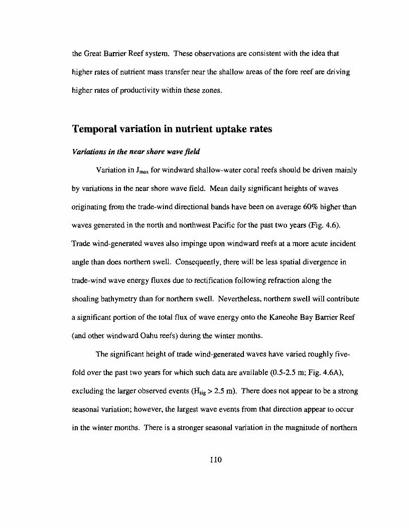
the Great Barrier Reef system. These observations are consistent with the idea that

higher rates of nutrient mass transfer near the shallow areas of the fore reef are driving

higher rates of productivity within these zones.

Temporal variation in nutrient uptake rates

Variations in the near shore wave field

Variation in Jm•• for windward shallow-water coral reefs should be driven mainly

by variations in the near shore wave field. Mean daily significant heights of waves

originating from the trade-wind directional bands have been on average 60% higher than

waves generated in the north and northwest Pacific for the past two years (Fig. 4.6).

Trade wind-generated waves also impinge upon windward reefs at a more acute incident

angle than does northern swell. Consequently, there will be less spatial divergence in

trade-wind wave energy fluxes due to rectification following refraction along the

shoaling bathymetry than for northern swell. Nevertheless, northern swell will contribute

a significant portion of the total flux of wave energy onto the Kaneohe Bay Barrier Reef

(and other windward Oahu reefs) during the winter months.

The significant height of trade wind-generated waves have varied roughly five­

fold over the past two years for which such data are available (0.5-2.5 m; Fig. 4.6A),

excluding the larger observed events (Hsig > 2.5 m). There does not appear to be a strong

seasonal variation; however, the largest wave events from that direction appear to occur

in the winter months. There is a stronger seasonal variation in the magnitude of northern

110

5,-------.----,--------,-----.----.---------,-----.----,

A4

....... 3E----Ol

'00:C2

1

0'-----'------'---'--------'----'--------'---'---....)JulOO OctOO Jan01 Apr01 Jul01 Ocl01 Jan02 Apr02 Jul02

5,------,-----,--------,r----,---.---------,,-----.------,

B4

....... 3E----Ol

'00:c 2

1

0'-----'------'---'--------'----'--------'---'---....)JulOO OclOO Jan01 Apr01 Jul01 OctO1 Jan02 Apr02 Jul02

Figure 4.6 (A) Daily mean significant height of trade wind-generated waves (30°to 150°) based on directional wave spectra measured -5 km off the MokapuPeninsula on the northeast coast of Oahu, Hawaii (21°24.9' N, 157°40.7 W) usinga Datawell, Inc, Waverider buoy, (B) Daily mean significant height of swellgenerated in the north and northwest Pacific (-75° to 30°), as measured by thesame buoy. Data courtesy of the University of Hawaii Sea Level Center andprocessed by P. Barraull.

III

swell observed off windward Oahu coasts (Fig. 4.6B), which, superimposed on the trade­

wind waves, implies generally higher fluxes of wave energy onto windward Oahu shores

during the winter. Unfortunately, it is not known how representative these patterns are

over longer periods of time (e.g., decades). For shallow-water waves, near-bottom

velocities should be roughly proportional to wave height and inversely proportional to the

square root of the water depth (Uh oc HIJh; Dean and Dalrymple 1991; see Chapter II).

The processes of shoaling, refraction, and breaking, as well as the substantial damping

effects of bottom friction, will affect the relative variation in near-bottom velocities and

Jrnax for a given reef community on windward Oahu. Nevertheless, simple wave theory

would suggest that the relative temporal variations in Jrnax for fore reef communities

should be comparable to that observed for significant wave heights.

Temporal variations in Jrnax for the Kaneohe Bay Barrier Reef flat are modulated

by the tide and wave heights outside Kaneohe Bay despite being strongly amplitude

filtered by depth-induced breaking (see Table 2.1, Chapter II). Estimates of S near the

surf zone varied by a factor of 2 over the sampled days while estimates at stations

furthers from the surf zone (400-500 m) varied by only a factor of 1.3. The days on

which these measurements were made correspond to significant wave heights (1.3 m - 1.9

m) which do not span the range of observed significant wave heights over the past two

years. 95% of all the daily average significant wave heights during the period of Aug

2000 through Jun 2002 fell between 0.5 and 3 m (data not shown). Therefore, variation

in Jrnax for the areas of the Kaneohe Bay Barrier Reef flat could be much greater than

1I2

reported here. However, given the distance over which most of the wave energy is

dissipated, it is likely that much of the reef flat experiences very little temporal variation

in Jm,x. On the other hand, deeper areas of the Kaneohe Bay Barrier Reef flat northwest

of Kapapa Island, as well as in areas close to the Sampan Channel, may observe

significant temporal variations in wave-driven flow speeds and nutrient uptake rates due

to increased wave transmittance.

The Kaneohe Bay Barrier Reef flat is anomalously wide (-2 km) in comparison

with most Indo-Pacific atolls, which are typically only -500 m wide (Kinsey 1979;

Wiens 1962). Consequently, cross-reef flow speeds on the Kaneohe Bay Barrier Reef

are much slower than those observed elsewhere (Atkinson I981b, 1987a; Bathen 1968;

Hearn and Parker 1988; Nelson 1996). Many Indo-Pacific atolls have shallow enough

reef crests to almost completely impede the passage of surface waves (Wiens 1962).

Under these circumstances, variations in U are driven by variations in wave heights

outside the reef due to changes in wave set up through the surf zone (Longuet-Higgins

and Stewart 1964; Tait 1972; Hearn and Parker 1988; Hearn 1999; Hearn et al. 2001;

Symonds et aI. 1995). Cross-reef currents resulting from this dynamic can vary between

a few centimeters per second to roughly a meter per second, which translate into

variations in Jmax of roughly an order of magnitude (Atkinson and Bilger 1992; Hearn and

Parker 1988). Therefore, variation in Jmax for many shallow-water reef communities are

greater than that of the Kaneohe Bay Barrier Reef flat.

It is clear that variations in the flow conditions over most reef communities are

driven by variations in the near shore wave field; regardless of whether flow is being

113

driven by the kinematics of the wave itself, or secondary currents set up by spatial

variation in wave heights.

Variability in nutrient concentrations

Rates of nutrient uptake by coral reef communities are mass transfer and thus

first-order with respect to nutrient concentration (Eqn. 4.2). Therefore, temporal

variations in Jmax should be linear with variations in nutrient concentrations. Continuous

records of dissolved inorganic nutrient concentrations inside and outside Kaneohe Bay

are available only from the end of 1998 through the middle of 2001 (Fig. 4.2), however,

concentrations reported over this period from outside the bay are comparable to those

reported during the late 1970s (Smith et al. 1981). Furthermore, concentrations reported

from water over the Kaneohe Bay Barrier Reef flat near the surf zone are close to those

reported from outside the bay (Atkinson 1981b; Atkinson, unpubl. data), while nutrient

concentrations in reef flat waters near the back reef are consistently low (Atkinson

1981b; Atkinson, unpubl. data). Nutrient concentrations in waters measured -10 km and

-100 km offshore of Oahu, Hawaii indicate vary little spatial gradient in dissolved

phosphate concentrations outside Kaneohe Bay (Fig. 4.2A), however, DIN concentrations

in waters farther offshore are lower by roughly an order of magnitude (Fig. 4.2B). This

may suggest that potential rates of DIN uptake for isolated, small atolls may be even

lower than estimates presented here since the concentrations of DIN to which fore reef

and reef flat communities at these atolls are exposed to may be closer to open ocean

values.

114

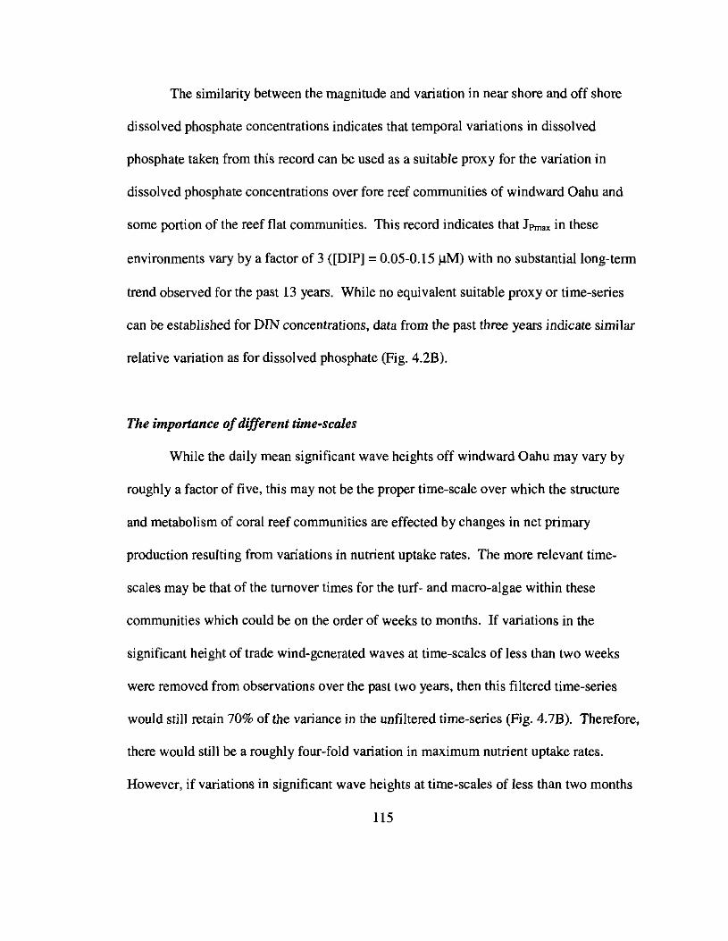
The similarity between the magnitude and variation in near shore and off shore

dissolved phosphate concentrations indicates that temporal variations in dissolved

phosphate taken from this record can be used as a suitable proxy for the variation in

dissolved phosphate concentrations over fore reef communities of windward Oahu and

some portion of the reef flat communities. This record indicates that JPmax in these

environments vary by a factor of 3 ([DIP] = 0.05-0.15 J.tM) with no substantial long-term

trend observed for the past 13 years. While no equivalent suitable proxy or time-series

can be established for DIN concentrations, data from the past three years indicate similar

relative variation as for dissolved phosphate (Fig. 4.2B).

The importance ofdifferent time-scales

While the daily mean significant wave heights off windward Oahu may vary by

roughly a factor of five, this may not be the proper time-scale over which the structure

and metabolism of coral reef communities are effected by changes in net primary

production resulting from variations in nutrient uptake rates. The more relevant time­

scales may be that of the turnover times for the turf- and macro-algae within these

communities which could be on the order of weeks to months. If variations in the

significant height of trade wind-generated waves at time-scales of less than two weeks

were removed from observations over the past two years, then this filtered time-series

would still retain 70% of the variance in the unfiltered time-series (Fig. 4.7B). Therefore,

there would still be a roughly four-fold variation in maximum nutrient uptake rates.

However, if variations in significant wave heights at time-scales of less than two months

115

A

B

5,---,-----,--------;,-------,---,--------;,---,----,

4

3

2

1

OL.---"-------'----'-------'-----'-------'-----'--_---.1

JulOO OctOO Jan01 Apr01 Jul01 OctO1 Jan02 Apr02 Jul02

5,-----,----,--------,---,----.-------,---,------,

4-E. 3OJ

r."' 2

1

OL.-_-L-_-----'__---'---_---'-__..I..-_--'--__L-_---.J

JulOO OctOO Jan01 Apr01 Jul01 Oct01 Jan02 Apr02 Jul02

5,---,--------,----,--,-------,---,------,------,

4 c3

2

1

O'----'---L-----'----_L-_----"-__--'-----_-----'-_----'Ju/OO OctOO Jan01 Apr01 Jul01 Ocl01 Jan02 Apr02 Jul02

Figure 4.7 Daily mean significant height of trade wind-generated wavesmeasured -5 Ian off the Mokapu Peninsula on the northeast of Oahu, Hawaii(21°24.9' N, 157°40.7' W). (A) Original time-series, (B) original time-series withvariations on time-scales of less than two-weeks removed, (C) original time-serieswith variations on time-scales of less than two months removed.

116

were removed, then this filtered time-series would retain only 20% of the variance

in the unfiltered time-series (Fig. 4.7C). This would represent a roughly two-fold

variation in maximum nutrient uptake rates. Clearly, the importance of temporal

variation in potential nutrient uptake rates must be considered with respect to the

time-scale of the organisms or communities which are effected by changes in net

primary production, e.g., the life-span of turf algae, macro-algae, coral, vertebrate

grazers (fishes), and invertebrate grazers.

117

v

CONCLUSIONS

Based on the preceding data and arguments, I conclude the following:

1) Rates of phosphate uptake by shallow « 2 m) communities are mass transfer

limited.

2) Rates of nutrient uptake to coral reef communities are 1.5-2 times higher under

wave-driven flows than under steady flows.

3) Shallow reef communities produce organic carbon via photosynthesis well in

excess of rates of net primary production which are allowed by mass transfer­

limited rates of nutrient uptake and relevant C:N:P ratios of reef autotrophs.

4) Spatial and temporal variation in nutrient uptake rates are driven by the near shore

wave climate and subsequent wave transformations.

5) Rates of nutrient uptake occurs at multiple roughness scales owing to the thinness

of the diffusive concentration boundary layer.

6) Rates of nutrient uptake by reef communities are 2-4 times higher than previously

estimated from mass transfer correlations.

118

REFERENCES

Atkinson, M. J. 1981a. Phosphate flux as a measure of net coral reef flat metabolism.

Fourth International Coral Reef Symposium. 1: 417-418.

Atkinson, M. J. 198Ib. Phosphate metabolism of coral reef flats. PhD Dissertation,

University of Hawaii. 90 pp.

Atkinson, M. J., and S. V. Smith. 1983. C:N:P ratios of benthic marine plants. Limno\.

Oceanogr. 28: 568-574.

Atkinson, M. J. 1987a. Rates of phosphate uptake by coral reef flat communities. Limno\.

Oceanogr. 32: 426-435.

Atkinson, M. J. 1987b. Alkaline Phosphatase activity of coral reef benthos. Coral Reefs.

6: 59-62.

Atkinson, M. J., and D. F. Smith. 1987. Slow uptake of 32p over a bamer reef flat.

Limno\. Oceanogr. 32: 436-44 I.

Atkinson, M. J. 1992. Productivity of Enewetak Atoll reef flats predicted flUm mass

transfer relationships. Cont. Shelf Res. 12: 799-807.

Atkinson, M. J., and R. W. Bilger. 1992. Effect of water velocity on phosphate uptake in

coral reef-flat communities. Limno\. Oceanogr. 37: 273-279.

Atkinson, M. J., E. Kottler, and P. Newton. 1994. Effects of water velocity on respiration,

calcification, and ammonium uptake of a Porites compressa community. Pacific

Sci. 48: 296-303.

Atkinson, M. J., J. L. Falter, and C. J. Hearn. 2001. Nutrient dynamics in the Biosphere 2

coral reef mesocosm: water velocity controls Nl1I and P04 uptake. Coral Reefs.

20: 341-346.

Baird, M. E., and M. J. Atkinson. 1997. Measurement and prediction of mass transfer to

experimental coral reef communities. Limnol. Oceanogr. 42: 1685-1693.

Barnes, D. J., and M. J. Devereux. 1984. Productivity and calcification on a coral reef: A

survey using pH and oxygen electrodes. J. Exp. Mar. BioI. Bco\. 79: 213-231.

Batchelor, G. K. 1967. The theory of homogenous turbulence. Cambridge University

119

Press.

Bathen, K. H. 1968. A descriptive study of the physical oceanography of Kaneohe Bay,

Hawaii. Masters Thesis, University of Hawaii. 353 pp.

Bilger, R. W., and M. 1. Atkinson. 1992. Anomalous mass transfer of phosphate on coral

reef flats. Limno!. Oceanogr. 37: 261-272.

Bilger, R. W., and M. J. Atkinson. 1995. Effects of nutrient loading on mass-transfer

rates to a coral-reef community. Limnol. Oceanogr. 40: 279-289.

Carpenter, R. C., J. M. Hackney, and W. H. Adey. 1991. Measurements of primary

productivity and nitrogenase activity of coral reef algae in a chamber

incorporating oscillatory flow. Limno!. Oceanogr. 36: 40-49.

Chun-Smith, A. A. 1994. The effects of nutrient loading on C:N:P ratios of marine

macroalgae in Kaneohe Bay, Hawaii. Masters Thesis, University of Hawaii. 80

pp.

Crossland, C. J., and D. J. Barnes. 1983. Dissolved nutrients and organic particulates in

water flowing over coal reefs at Lizard Island. Austr. J. Mar. Freshw. Res. 34:

835-844.

Crossland, C. J., B. G. Hatcher, M. J. Atkinson, and S. V. Smith. 1984. Dissolved

nutrients of a high-latitude reef, Houtman Abrolhos Islands, Western Australia.

Mar. Eco!. Prog. Ser. 14: 159-163.

Crossland, C. J., B. G. Hatcher, and S. V. Smith. 1991. Role of coral reefs in global ocean

production. Coral reefs. 10: 55-64.

Culberson, C. H., G. Latham, and R. G. Bates. 1978. Solubilities and activity coefficients

of calcium and strontium sulfates in synthetic seawater at 0.5 and 25 deg C. J.

Phys. Chern. 82: 2693-2699.

Dade, W. B. 1993. Near-bed turbulence and hydrodynamic control of diffusional mass

transfer at the sea floor. Limno!. Oceanogr. 38: 52-69.

Darwin, C. 1842. The structure and distribution of coral reefs. University of California

Press. 214 pp.

Dawson, D. A., and O. Trass. 1972. Mass transfer at rough surfaces. In!. J. Heat Mass

120

Transfer. 15: 1317-1336.

Dean, R. G., and R. A. Dalrymple. 1991. Water wave mechanics for engineers and

scientists. World Scientific Publishing. 353 pp.

D'Elia, C. F. 1977. The uptake and release of dissolved phosphorus by reef corals.

Limnol. Oceanogr. 22: 301-315.

Dipprey, D. F., and R. H. Sabersky. 1963. Heat and momentum transfer in smooth and

rough tubes at various Prandtl numbers. Int. J. Heat Mass Transfer. 6: 329-353.

Doty, M. S. 1971. Measurement of water movement in reference to benthic algal growth.

Bot. Mar. 14: 4-7.

Gaylord, B., C. A. Blanchette, and M. W. Denny. 1994. Mechanical consequences of

wave-swept algae. Ecol. Monogr. 64: 287-313.

Gerritsen, F. 1981. Wave attenuation and wave set-up on a coastal reef. Ph.D.

Dissertation, University of Trondheim. 416 pp.

Glynn, P. W. 1973. Ecology of a Caribbean coral reef. The Porites reef-flat biotope: part

II. Plankton community with evidence for depletion. Mar. BioI. 22: 1-21.

Gourlay, M. R. 1994. Wave transformation on a coral reef. Coastal Eng. 23: 17-42.

Haaland, S. E. 1983. Simple and explicit formulas for the friction factor in turbulent pipe

flow. J. Fluids Eng. 105: 89-90.

Hardy, T. A., and I. R. Young. 1996. Field study of wave attenuation on an offshore coral

reef. J. Geophys. Res. 101: 14,311-14,326.

Hearn, C. J., and I. N. Parker. 1988. Hydrodynamic processes on the Ningaloo coral reef,

Western Australia. 6th International Coral Reef Symposium. 2: 497-502.

Hearn, C. J. 1999. Wave-breaking hydrodynamics within coral reef systems and the

effect of changing sea level. J. Geophys. Res. 104: 30,007-30,019.

Hearn, C. 1. 2001. Roughness and the dynamics of waves, turbulence, and currents on

nearshore reefs. Eos Trans., AGU. 82: Fall Meet. Suppl., Abstract OS 12A-0407.

Hearn, C. J., M. J. Atkinson, and J. L. Falter. 2001. A physical derivation of nutrient­

uptake rates in coral reefs: effects of roughness and waves. Coral Reefs. 20: 347­

356.

121

Horikawa, K. 1988. Nearshore dynamics and coastal processes. University of Tokyo

Press. pp.

Isobe, M. 1983. Long period field observation on horizontal distribution of waves and

currents in the nearshore zone. NERC, 17-34 pp.

Isobe, M. 1985. Calculations and application of first-order cnoidal wave theory. Coastal

Eng. 9: 309-325.

Jensen, B. J. 1989. Experimental investigation of turbulent oscillatory boundary layers.

Institute of Hydraulic and Hydrodynamic Engineering (ISVA), Technical

University of Denmark, pp.

Johannes, R. E., J. Alberts, C. D'Elia, R. A. Kinzie, L. R. Pomeroy, W. Sottile, W.

Wiebe, J. A. J. Marsh, P. Helfrich, J. Maragos, J. Meyer, S. V. Smith, D.

Crabtree, A. Roth, L. R. McCloskey, S. Betzer, N. Marshall, M. E. Q. Pilson, G.

Telek, R. I. Clutter, W. D. DuPaul, K. L. Webb, and J. M. 1. Wells. 1972. The

metabolism of some coral reef communities: A team study of nutrient and energy

fluxes. Bioscience. 22: 541-543.

Johannes, R. E., W. J. Wiebe, and C. J. Crossland. 1983. Three patterns of nutrient flux in

a coral reef community. Mar. Bco!. Prog. Ser. 12: 131-136.

Jokiel, P. L., and J. I. Morrisey. 1993. Water motion on coral reefs: evaluation of the

'clod card' technique. Mar. Eco!. Prog. Ser. 93: 175-181.

Jonsson, I. G. 1966. Wave boundary layers. 10th Coastal Engineering Conference. 127­

148.

Jonsson, I. G. 1980. A new approach to oscillatory rough turbulent boundary layers.

Ocean Eng. 7: 109-152.

Kajiura, K. 1968. A model of the bottom boundary layer in waves. Bul!. Earthquake Res.

Inst. 46: 75-123.

Kamphuis, J. W. 1975. Friction factors under oscillatory waves. J. Waterway Harbours

Coastal Engineering Division, ASCE. 101: 135-144.

Kays, W. M., and M. E. Crawford. 1993. Convective Heat and Mass Transfer. McGraw­

Hill. 601 pp.

122

Kemp, P. H., and R. R. Simons. 1983. The interaction between waves and a turbulent

current: waves propagating with the current. J. Fluid Mech. 116: 227-250.

Kinsey, D. W. 1979. Carbon turnover and accumulation by coral reefs. PhD Dissertation,

University of Hawaii. 248 pp.

Kinsey, D. W. 1985. Metabolism, calcification, and carbon production: I. Systems level

studies. Fifth International Coral Reef Congress. 4: 505-526.

Kinzie III, R. A., F. T. Mackenzie, S. V. Smith, and J. Stimson. 2001. CISNe!: linkages

between a tropical watershed and reef ecosystems. NOAA, Honolulu. pp.

Krumgalz, B. S., and F. J. Millero. 1982. Physico-chemical studies of the Dead Sea

waters I. Activity coefficients of major ions in Dead Sea Water. Mar. Chern. 11:

209-222.

Krumgalz, B. S., and F. J. Millero. 1983. Physico-chemical study of dead sea waters. III.

On gypsum saturation in Dead Sea waters and their mixtures with Mediterranean

Sea water. Mar. Chem.13: 127-139.

Kundu, P. J. 1990. Fluid Mechanics. Academic Press. 638 pp.

Lamed, S. T., and M. J. Atkinson. 1997. Effects of water velocity on N~ and PO. uptake

and nutrient-limited growth in the macroalgae Dictyosphaeria cavernosa. Mar.

Ecol. Prog. Ser. 157: 295-302.

Li, Y.-H., and S. Gregory. 1974. Diffusion of ions in sea water and in deep-sea

sediments. Geochim. Cosmochim. Acta. 38: 703-714.

Lide, D. R. (Ed.). 2000. CRC Handbook of Chemistry and Physics. CRC Press. pp.

Longuet-Higgins, M. S., and R. W. Stewart. 1964. Radiation stress in water waves; a

physical discussion with applications. Deep-Sea Res. 11: 529-562.

Lugo-Fernandez, A., H.H. Roberts, and J. N. Suhayda. 1998a. Wave transformations

across a Caribbean fringing-barrier coral reef. Cont. Shelf. Res. 18: 1099-1124.

Lugo-Fernandez, A., H.H. Roberts, and W.J. Wiseman, Jr. 1998b. Tide effects on wave

attenuation and wave set-up on a Caribbean coral reef. Est., Coastal, and Shelf

Sci. 47: 385-393.

Masse!, S. R., and M. R. Gourlay. 2000. On the modeling of wave breaking and set-up on

123

coral reefs. Coastal Eng. 39: 1-27.

Morel, F. M. M. 1983. Principles of Aquatic Chemistry. John Wiley & Sons, Inc. 446 pp.

Munk, W. H., and M. C. Sargent. 1954. Adjustment of Bikini Atoll to ocean waves. U.S.

Geo!. SUTY., 275-280 pp.

Muscatine, L., and C. F. D'Elia. 1978. The uptake, retention, and release of ammonium

by reef corals. Limno!. Oceanogr. 23: 725-734.

Muus, B. 1968. A field method for measuring "exposure" by means of plaster balls, a

preliminary account. Sarsia. 34: 61-68.

Nelson, R. C. 1996. Hydraulic roughness of coral reef platforms. Appl. Ocean Res. 18:

265-274.

Nielsen, P. 1992. Coastal bottom boundary layers and sediment transport. World

Scientific Publishing. 324 pp.

Odum, H. T., and E. P. Odum. 1955. Trophic structure and productivity of a windward

coral reef community on Eniwetok Atoll. Eco!. Monogr. 25: 1415-1444.

Odum, H. T. 1971. Fundamentals of Ecology. W.B. Saunders Co. 574 pp.

Pilson, M. E. Q., and S. B. Betzer. 1973. Phosphorus flux across a coral reef. Ecology.

54: 1459-1466.

Porter, E. T., L. P. Sanford, and S. E. Suttles. 2000. Gypsum dissolution is not a universal

indicator of 'water motion'. Limnol. Oceanogr. 45: 145-158.

Pytkowicz, R. M., and J. E. Hawley. 1974. Bicarbonate and carbonate ion-pairs and a

model of seawater at 25 degrees C. Limnol. Oceanogr. 19: 223-234.

Raubenheimer, B., R. T. Guza, and S. Elgar. 1996. Wave transformation across the inner

surf zone. J. Geophys. Res. 101: 25,589-25,597.

Riedel, H. P. 1972. Direct measurement of bed shear stress under waves. Dissertation,

Queen's University. pp.

Santschi, P. H., R. F. Anderson, M. Q. Fleisher, and W. Bowles. 1991. Measurements of

diffusive sublayer thickness in the ocean by alabaster dissolution, and their

implications for the measurement of benthic fluxes. J. Geophys. Res. 96: 10,641­

10,657.

124

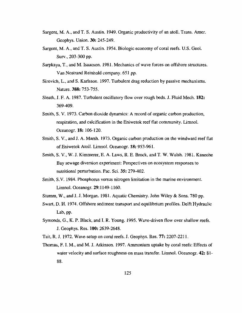
Sargent, M. A., and T. S. Austin. 1949. Organic productivity of an atoll. Trans. Amer.

Geophys. Union. 30: 245-249.

Sargent, M. A., and T. S. Austin. 1954. Biologic economy of coral reefs. U.S. Geol.

Surv., 203-300 pp.

Sarpkaya, T., and M. Isaacson. 1981. Mechanics of wave forces on offshore structures.

Van Nostrand Reinhold company. 651 pp.

Sirovich, L., and S. Karlsson. 1997. Turbulent drag reduction by passive mechanisms.

Nature. 388: 753-755.

Sleath, J. F. A. 1987. Turbulent oscillatory flow over rough beds. J. Fluid Mech. 182:

369-409.

Smith, S. V. 1973. Carbon dioxide dynamics: A record of organic carbon production,

respiration, and calcification in the Eniwetok reef flat community. Limnol.

Oceanogr. 18: 106-120.

Smith, S. V., and J. A. Marsh. 1973. Organic carbon production on the windward reef flat

of Eniwetok Atoll. LimnoJ. Oceanogr. 18: 953-961.

Smith, S. V., W. J. Kimmerer, E. A. Laws, R. E. Brock, and T. W. Walsh. 1981. Kaneohe

Bay sewage diversion experiment: Perspectives on ecosystem responses to

nutritional perturbation. Pac. Sci. 35: 279-402.

Smith, S.V. 1984. Phosphorus versus nitrogen limitation in the marine environment.

Limnol. Oceanogr. 29:1149-1160.

Stumm, W., and J. J. Morgan. 1981. Aquatic Chemistry. John Wiley & Sons. 780 pp.

Swart, D. H. 1974. Offshore sediment transport and equilibrium profiles. Delft Hydraulic

Lab, pp.

Symonds, G., K. P. Black, and I. R. Young. 1995. Wave-driven flow over shallow reefs.

J. Geophys. Res. 100: 2639-2648.

Tait, R. J. 1972. Wave-setup on coral reefs. J. Geophys. Res. 77: 2207-2211.

Thomas, F. I. M., and M. J. Atkinson. 1997. Ammonium uptake by coral reefs: Effects of

water velocity and surface roughness on mass transfer. Limnol. Oceanogr. 42: 81­

88.

125

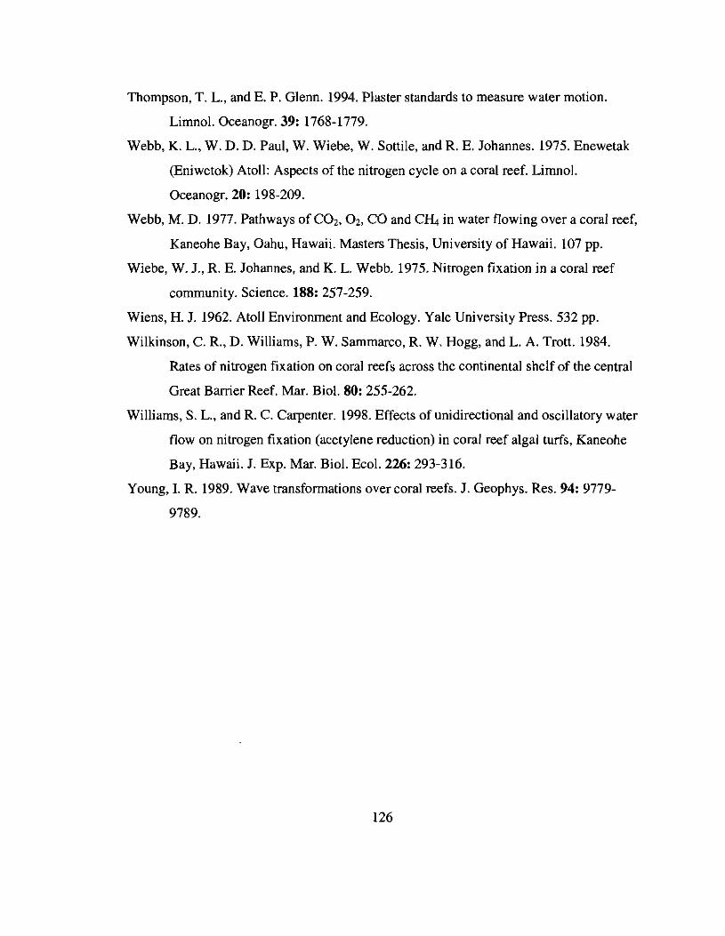
Thompson, T. L., and E. P. Glenn. 1994. Plaster standards to measure water motion.

Limnol. Oceanogr. 39: 1768-1779.

Webb, K. L., W. D. D. Paul, W. Wiebe, W. Sottile, and R. E. Johannes. 1975. Enewetak

(Eniwetok) Atoll: Aspects of the nitrogen cycle on a coral reef. Limnol.

Oceanogr. 20: 198-209.

Webb, M. D. 1977. Pathways of CO2, 02, CO and CIil in water flowing over a coral reef,

Kaneohe Bay, Oahu, Hawaii. Masters Thesis, University of Hawaii. 107 pp.

Wiebe, W. J., R. E. Johannes, and K. L. Webb. 1975. Nitrogen fixation in a coral reef

community. Science. 188: 257-259.

Wiens, H. J. 1962. Atoll Environment and Ecology. Yale University Press. 532 pp.

Wilkinson, C. R., D. Williams, P. W. Sammarco, R. W. Hogg, and L. A. Trott. 1984.

Rates of nitrogen fixation on coral reefs across the continental shelf of the central

Great Barrier Reef. Mar. BioI. 80: 255-262.

Williams, S. L., and R. C. Carpenter. 1998. Effects of unidirectional and oscillatory water

flow on nitrogen fixation (acetylene reduction) in coral reef algal turfs, Kaneohe

Bay, Hawaii. J. Exp. Mar. BioI. Ecol. 226: 293-316.

Young, 1. R. 1989. Wave transformations over coral reefs. J. Geophys. Res. 94: 9779­

9789.

126