Size-Restricted Proton Transfer within Toluene-Methanol Cluster Ions
Upload
khangminh22Category
view
3download
0
HAL Id: tel-01920302https://hal.univ-lorraine.fr/tel-01920302
Submitted on 22 Jun 2020
HAL is a multi-disciplinary open accessarchive for the deposit and dissemination of sci-entific research documents, whether they are pub-lished or not. The documents may come fromteaching and research institutions in France orabroad, or from public or private research centers.
L’archive ouverte pluridisciplinaire HAL, estdestinée au dépôt et à la diffusion de documentsscientifiques de niveau recherche, publiés ou non,émanant des établissements d’enseignement et derecherche français ou étrangers, des laboratoirespublics ou privés.
Mass transfer within complex media. ReverseEngineering : from usage property to material
Antonio Aguilera Miguel
To cite this version:Antonio Aguilera Miguel. Mass transfer within complex media. Reverse Engineering : from us-age property to material. Chemical engineering. Université de Lorraine, 2018. English. NNT :2018LORR0046. tel-01920302

AVERTISSEMENT
Ce document est le fruit d'un long travail approuvé par le jury de soutenance et mis à disposition de l'ensemble de la communauté universitaire élargie. Il est soumis à la propriété intellectuelle de l'auteur. Ceci implique une obligation de citation et de référencement lors de l’utilisation de ce document. D'autre part, toute contrefaçon, plagiat, reproduction illicite encourt une poursuite pénale. Contact : [email protected]
LIENS Code de la Propriété Intellectuelle. articles L 122. 4 Code de la Propriété Intellectuelle. articles L 335.2- L 335.10 http://www.cfcopies.com/V2/leg/leg_droi.php http://www.culture.gouv.fr/culture/infos-pratiques/droits/protection.htm

LRGP-CNRS UMR 7274Laboratoire Réactions et Génie des ProcédésCentre National de la recherche scientifiqueRessources Procédés Produits Environnement
THÈSE
Présentée pour obtenir le grade de
Docteur en Génie des Procédés et des Produits
le 15 Mai 2018 à Nancy
Par
Antonio AGUILERA MIGUEL
TRANSFERT DE MATIÈRE DANS LES MILIEUX COMPLEXES.
INGÉNIERIE INVERSE: DE LA PROPRIÉTÉ D’USAGE AU MATÉRIAU
Directeur: Pr. Christophe CASTEL
Codirecteurs: Pr. Véronique SADTLER et Dr. Philippe MARCHAL
Composition du Jury:
Examinateur: Dr. Véronique SCHMITT
Rapporteurs: Pr. Raffaella OCONE et Pr. Jack LEGRAND

2
Résumé élargi
La maîtrise des phénomènes de transfert de masse est une condition impérative pourl’élaboration et l’utilisation des produits formulés. L’objectif principal de cette thèse estle développement d’une ingénierie inverse appliquée à l’ingénierie des produits chimiques.Contrairement à l’ingénierie prospective, l’ingénierie inverse est généralement définie commele processus d’examen d’un système déjà mis en œuvre afin de le représenter sous une formeou un formalisme différent et à un niveau d’abstraction plus élevé. La notion clé est celle dereprésentation, qui peut être associée au concept de modèle au sens large du terme. L’objectifde ces représentations est de mieux comprendre l’état actuel d’un système, par exemplepour le corriger, le mettre à jour, le mettre à niveau, en réutiliser des parties dans d’autressystèmes, ou même le réinventer complètement. Le concept existe depuis longtemps avant lesordinateurs ou la technologie moderne, et remonte probablement à l’époque de la révolutionindustrielle.
Traditionnellement, l’ingénierie inverse a consisté à prendre des produits et à les disséquerphysiquement pour découvrir les secrets de leur conception. Ces secrets étaient alors générale-ment utilisés pour fabriquer des produits similaires ou meilleurs. Elle est généralement menéepour obtenir les connaissances, les idées et la philosophie de conception manquantes lorsqueces informations ne sont pas disponibles. Dans certains cas, l’information appartient àquelqu’un qui n’est pas disposé à la partager. Dans d’autres cas, l’information a été perdueou détruite. De toute évidence, l’application la plus connue de l’ingénierie inverse est ledéveloppement de produits concurrents. Ce qui est intéressant, c’est qu’il n’est pas aussipopulaire dans l’industrie qu’on pourrait s’y attendre. C’est principalement parce qu’onpense qu’il s’agit d’un processus tellement complexe qu’il n’a tout simplement pas de senssur le plan financier, ainsi qu’un processus long et sujet aux erreurs.
Au cours de la dernière décennie, l’utilisation croissante de nombreuses technologiesnouvelles en tant que systèmes de livraison contrôlée a donné lieu à des essais et des erreurscoûteux pour la mise au point de systèmes nouveaux et efficaces. Afin de faciliter uneconception et une optimisation plus rationnelle, face à l’ensemble des possibilités existantes,toute solution d’ingénierie inverse qui pourrait semi-automatiser le développement du produitapporterait une aide précieuse aux utilisateurs (scientifiques et éducateurs). Cela faciliteraitl’importance essentielle de choisir les bons matériaux pour l’application correcte.
L’objectif de la thèse est de développer une méthodologie pour l’ingénierie de conceptiondu produit basée sur l’ingénierie inverse afin de déterminer la formulation optimale à partird’une propriété d’utilisation finale donnée, ici la libération contrôlée. La thèse est divisée enquatre chapitres, suivis d’une conclusion finale et de perspectives.

3
Le premier chapitre est consacré à l’approche de l’ingénierie inverse. L’ingénieriedes produits chimiques est définie par la conversion des besoins des clients en produitschimiques en maîtrisant la formulation et les interactions avec le processus. Les objectifs del’ingénierie des produits chimiques tels que définis dans la littérature peuvent être décrits encinq étapes : 1) conversion des besoins des consommateurs aux spécifications techniques ; 2)modélisation et optimisation, conception assistée par ordinateur ; 3) capacités prédictivespour les propriétés physiques avec l’utilisation de la thermodynamique appliquée ; 4) cadresystématique et intégré pour la conception de nouveaux produits ; 5) cadre pour lier ladécouverte de produits aux efforts de R-D.
Un état de l’art des technologies de libération contrôlée est présenté dans ce chapitre.Différents nanoporteurs pharmaceutiques polymériques peuvent être utilisés : micellespolymères, nanocapsules, nanogels polymères, polymères, polymères ramifiés (dendrimères),nanoparticules hybrides à noyaux poreux. Pour les applications alimentaires, le type de cap-sules dépend de la nature des composés encapsulés. Pour les composés hydrophobes, on peututiliser des émulsions (micro-émulsions, émulsions de Pickering) ou des supports lipidiquesnanostructurés. Pour les composés hydrophiles, hydrogels, liposomes, colloïdosomes, colloï-dosomes sont les différentes possibilités d’encapsulation. Il y a quatre principaux mécanismesde libération : contrôlé par diffusion, contrôlé par solvant, contrôlé par réaction chimique etcontrôlé par stimuli.
La prédiction de la libération contrôlée dépend bien sûr du mécanisme en cause. Certaineséquations empiriques existent, comme l’équation de Peppas. Le modèle de Hopfenberg estégalement un modèle empirique, capable de prendre en compte la dissolution, le gonflementet le clivage de la chaîne polymère. Un complément du dernier modèle est le modèle Cooney,qui tient compte de la géométrie des capsules. Le dernier modèle empirique est basé surdes réseaux neuronaux artificiels. Les modèles mécanistes sont généralement basés sur deséquations de transfert de masse.
La deuxième loi de Fick est la base des phénomènes de diffusion. Si l’intégrité descapsules demeure, certaines expressions donnant la cinétique de la libération du médicamentpeuvent être trouvées dans la littérature, soit pour les réservoirs de médicaments, soit pour lesdispositifs monolithiques. Pour les phénomènes de gonflement des polymères, la diffusionde l’eau dépend également de la deuxième loi de Fick, tout comme pour la diffusion dumédicament. En cas de gonflement du polymère et de dissolution du médicament, le modèlede couche séquentielle est appliqué. La deuxième loi de Fick est utilisée avec des coefficientsde diffusion non constants, qui sont décrits par une dépendance exponentielle de type Fujita,à la fois pour la diffusion de l’eau et de la drogue. Pour la dissolution, la cinétique de pertede masse du polymère est également prise en compte. Enfin, pour l’érosion/dégradation

4
des polymères, deux types de phénomènes d’érosion, en surface ou en volume, peuvent seproduire en fonction de la cinétique de clivage de la chaîne polymère par rapport à la cinétiquede pénétration de l’eau. La cinétique de libération tient compte du front d’érosion. Le clivagede la chaîne polymère est un processus aléatoire qui pourrait être simulé par l’approche deMonte Carlo. Le processus de transport de masse est représenté par la deuxième loi de Ficktridimensionnelle.
La conclusion du chapitre est la description du cadre de rétro-ingénierie. Elle commencepar le domaine d’application (profil de produit cible) et les principes actifs correspondants.Ensuite, la deuxième étape est l’étude de la thermodynamique et des équilibres de phase,suivie d’un traitement de formulation pour obtenir un système dispersé avec des caractéris-tiques spécifiques. Ensuite, on procède à la modélisation théorique et à la simulation de lacinétique de libération. La dernière étape est le travail expérimental afin de tester la meilleuresolution et de vérifier et améliorer les simulations.
Le chapitre 2 est consacré à l’établissement d’un modèle de transfert de masse sansparamètres d’ajustement. Le modèle de système est l’émulsion, car il est adapté à laréalisation de systèmes de distribution. Une partie de ce chapitre correspond à un articlepublié dans Colloïdes et Surfaces A. L’objectif de l’article est d’étudier la stabilisation del’huile hautement concentrée dans les émulsions aqueuses (jusqu’à 94%) par des dextransmodifiés hydrophobiquement. Ces stabilisateurs permettent une longue stabilité sur l’échellede temps malgré une cinétique plus lente, des tailles de gouttelettes plus élevées et destensions de surface plus élevées que les autres stabilisateurs commerciaux.
Les objectifs du chapitre sont de modéliser un système pour les applications d’administrationen considérant les émulsions hautement concentrées comme système modèle. Pour le fluxde masse, la résistance au transfert de masse est localisée dans la couche de tensioactif,caractérisée par la perméabilité, et dans le film en phase continue autour de la gouttelette,caractérisé par un coefficient de transfert de masse. La perméabilité est obtenue à partirdu produit entre la perméabilité d’une couche de désordre et un facteur représentant ladiminution de la perméabilité due à l’ordre interfacial. Un domaine de variation est donnépour le coefficient de transfert de masse interfaciale dans le cas où l’épaisseur du film enphase continue est inconnue, ce qui est souvent le cas. Le coefficient de diffusion peut êtreestimé à partir de l’équation de Stokes-Einstein ou d’équations empiriques. Le coefficient departage à l’équilibre thermodynamique peut être calculé à partir des coefficients d’activité.
Ces propriétés thermodynamiques peuvent être estimées à partir de techniques de con-ception moléculaire assistée par ordinateur (CAMD). Différentes techniques ont été utiliséesdans ce travail. Parmi eux, il y a le modèle UNIFAC (Functional-group Activity Coefficients),qui permet de prédire le coefficient d’activité en phase liquide. Le modèle a une contribution

5
combinatoire au coefficient d’activité due aux différences de taille et de forme des molécules,et une contribution résiduelle due aux interactions énergétiques. Un modèle UNIFAC modifié(Dortmund) est proposé pour tenir compte des composés de taille très différente en changeantempiriquement la partie combinatoire. En raison de certains inconvénients du modèle UNI-FAC, modifié ou non, en raison de l’absence de certains paramètres d’interaction binaires,l’utilisation du COSMOS-RS (Conductor-like Screening Model for Real Solvents) est utilepour l’évaluation de l’interaction moléculaire dans les liquides et, ensuite, pour fournir desdonnées supplémentaires pour le modèle UNIFAC modifié. Le modèle ainsi obtenu estappelé Révision et extension 6 du modèle modifié d’UNIFAC (Dortmund). La prédiction del’équilibre liquide-liquide permet de calculer les deux compositions de phase au moyen d’uneméthode itérative de bissection, y compris le calcul des coefficients d’activité et l’intégrationd’un bilan massique.
La méthode VABC (Atomic and Bond Contributions of van der Waals volume) est utiliséepour le calcul des volumes moléculaires. La viscosité du mélange liquide est calculée par unmodèle UNIFAC modifié (UNIFAC-VISCO). Le volume molaire liquide au point d’ébullitionnormal est calculé (méthode Tyn et Callus) à partir du volume critique, qui est calculé parune méthode de contribution de groupe (méthode Joback). Le modèle de transfert de massetient compte de la diffusion dans la gouttelette, à travers le film interfacial et dans la phasecontinue et l’équation résultante est basée sur la seconde loi de Fick.
Le troisième chapitre est consacré à la simulation. La première partie consiste en unevue d’ensemble du modèle ab-initio développé dans la thèse pour prédire la libération d’unprincipe actif à partir de l’eau dans des émulsions fortement concentrées dans l’huile avec lesmodèles détaillés au chapitre 2. Le modèle ab initio est développé sur MATLAB pour prédirele débit instantané de l’ingrédient actif dans les deux phases et son profil de pourcentagecumulatif.
Une analyse des structures moléculaires d’éventuels produits chimiques candidats est en-suite donnée afin de créer une cartographie des matériaux avec lesquels travailler. L’ingrédientactif choisi est l’acide mandélique. La phase dispersée est l’eau avec parfois une certainequantité d’électrolyse (NaCl), ce qui augmente la stabilité de l’émulsion. Pour la phasecontinue, quatre huiles différentes ont été choisies, deux n-alcanes saturés (dodécane et hex-adécane) et deux esters d’acides gras (myristate d’isopropyle et palmitate d’isopropyle). Troistypes différents d’agents tensioactifs ont été choisis, avec un HLB (équilibre hydrophile-lipophile) approprié par rapport aux huiles choisies. Ce sont : un ester d’acide gras desorbitane (monooléate de sorbitane, SPAN 80), un acide gras polyglycérisé (polyricinoléatede polyglycérol, PGPR) et un éther alkylique de polyéthylène glycol (polyoxyéthylèneglycol-2-oléyléther, BRIJ 93).

6
Une bonne initiative consiste à proposer une analyse de sensibilité des variables. Lemodèle ab-initio est utilisé pour réaliser des expériences virtuelles et le plan d’expériencesvirtuel (VDOE) permet de revoir l’interaction entre les variables du processus. Un planfactoriel de 64 combinaisons est d’abord analysé. Le diagramme de Pareto montre quele facteur le plus influent est la fraction de masse en phase dispersée, suivie du choix dusurfactant. Au contraire, la concentration de l’ingrédient actif et le diamètre des gouttelettesont une influence moins importante et peuvent être négligés pour des analyses futures.
Pour une analyse plus approfondie, seules quatre variables (fraction de masse en phasedispersée, rapport huile-surfactant, type d’huile, type d’huile, type de surfactant) ont étéconservées pour une conception factorielle de 300 combinaisons. Le coefficient de diffu-sion diminue linéairement avec la fraction de masse en phase dispersée, qui est le facteurd’influence le plus important. Le rapport huile-surfactant n’a pas d’effet. L’huile de palmitateet le SPAN 80 donnent le coefficient de diffusion le plus bas. De plus, les interactions lesplus prononcées de la fraction de masse dispersée sont liées au choix de l’huile ou de l’agenttensioactif, en particulier pour les faibles fractions.
Le dernier chapitre donne la validation expérimentale. Le premier point est la com-paraison des coefficients de distribution prévus et expérimentaux. Les résultats montrentque la meilleure prédiction est donnée par la révision et l’extension 6 du modèle UNIFACmodifié (Dortmund). On sait que le modèle classique de l’UNIFAC est davantage consacré àl’équilibre vapeur-liquide. Un problème est le fait que, pendant les expériences, une troisièmephase (un film nuageux) apparaît à l’interface. Cette troisième phase n’est pas prise en comptedans le modèle, et peut perturber la détermination de l’ingrédient actif, qui se fait par uneconférence sur l’absorption des UV. Cependant, la présence de sel permet d’améliorer laprédiction, car le film interfacial devient plus étroit. La prédiction est également moins bonnepour le tensioactif BRIJ 93, mais il semble très compliqué de donner une raison justifiant cefait en raison de déviations expérimentales.
La prédiction par la méthode UNIFAC-VISCO des viscosités du mélange est en ac-cord avec les viscosités expérimentales pour la diminution avec l’augmentation du rapporthuile/factant. Les viscosités sont largement plus élevées avec le tensioactif PGPR, mais lesvaleurs prévues et expérimentales présentent des différences significatives, peut-être dues àla formation de micelles dans ce cas.
Pour la comparaison de la cinétique de libération, les émulsions ont été préparées avecdes diamètres de gouttelettes allant de 8 à 19 (µm). Une comparaison entre les courbesde libération prévue et expérimentale est faite pour les différentes phases huileuses et lessurfactants. Certaines similitudes et différences apparaissent. La comparaison entre lecoefficient de diffusion prévu et le coefficient de diffusion expérimental montre qu’un

7
meilleur accord est obtenu pour les émulsions préparées avec des huiles de dodécane etd’hexadécane avec SPAN 80® et PGPR® comme surfactants. Une discussion sur la raisonde ce résultat devrait être utile pour la mise en œuvre de cette approche à d’autres systèmes.Les écarts entre les coefficients de diffusion expérimental et prédit sont relativement biencorrélés avec les écarts observés pour les modules de stockage expérimental et prédit.
La dernière partie du chapitre est un rapport d’analyse en composantes principales pourvisualiser l’importance des variables. Le film interfacial et le coefficient de partage ont unrôle clé. La viscosité de la phase continue a un effet sur la cinétique de libération, qui pourraitêtre contrôlée par l’ajout d’épaississants. Certaines différences entre les prédictions et lesexpériences peuvent s’expliquer par la grande perméabilité de certains tensioactifs, commepar exemple le BRIJ 93®, car, dans ce cas, un transfert de masse rapide à travers la couchede tensioactif pourrait modifier les paramètres structurels en un temps plus court, conduisantalors à des instabilités non prises en compte dans le modèle.
Cette thèse est la première étape d’un projet à long terme sur la rétroingénierie appliquéeà la conception de produits. Quelle est la formulation optimale pour obtenir une propriétéd’utilisation finale? Cette question peut être résolue en utilisant la méthodologie développéedans ce travail pour les émulsions hautement concentrées, en ajoutant des critèries commer-ciales. Des modèles constitutifs ont été établis pour prédire le transfert de masse de la matièreactive en fonction des paramètres de formulation, y compris des techniques assistées parordinateur comme la modélisation moléculaire, ou des modèles UNIFAC pour les prévisionsd’équilibre liquide-liquide et pour l’estimation de la viscosité des mélanges. L’approched’ingénierie inverse est vraiment très intéressante pour l’ingénierie de conception de produitspour le criblage rapide possible des différentes variables influençant la cinétique de libération.Une perspective importante est d’appliquer la même méthodologie à d’autres systèmes dedissémination contrôlée.


Acknowledgements
Firstly, I would like to express my sincere gratitude to my supervisors Christophe Castel,Véronique Sadtler and Philippe Marchal for the continuous support of my Ph.D study andrelated research, for their patience, motivation, and immense knowledge. Their guidancehelped me in all the time of research and writing of this thesis. I could not have imaginedhaving better advisors and mentors for my Ph.D study.My sincere thanks also goes to Lionel Choplin, who provided me an opportunity to join theirteam, and who gave access to the laboratory and research facilities. Without its precioussupport, together with Josiane Moras, it would have not been possible to conduct this re-search. A very special gratitude goes out to the Ministère de l’Enseignement Supérieur de laRecherche et de la l’Innovation, for helping and providing the funding for the work.To Charly Koenig and Herve Simonaire, who helped me on the design of the pilot plant andduring troubleshooting, to Sébastien Kiesgen de Richter and co-workers from LEMTA labo-ratory, who allowed me to use their technique of incoherent polarized steady light transport(AIPSLT) for emulsion characterization in my work. I extend my deepest appreciation fortheir helpful and expert advice, guidance, and encouragement.I am also very indebted to Edeluc López-Gonzalez, Hala Fersadou and Emilio Paruta-Tuarez,because their previous work in the laboratory inspired me and helped me for the developmentof my thesis in the beginning.I thank my fellow labmates; Eve Masurel, Yaoh, Katja Huys, Mégane Poirson, Anne-LaureBagard, Arvind Krishnan, Jiaqi Dong, Darkhan Zholtayev, Aikumis Serikbayeva, CarolineBottelin, Assia Saker, Benjamin Lhuizière and Martin Meulders for all the stimulating dis-cussions and accompaniment, specially Mahbub Morshed for the sleepless nights we wereworking together before deadlines, and generally to all of them for the fun we have had inthe last years. Also I thank my colleagues and professors from the University of Huelva. Inparticular, I am grateful to Crispulo Gallegos for enlightening me the first glance of researchduring my life, and being my mentor since I left the university.Last but not the least, I would like to thank my family: my parents Antonio and Mª Carmen,and to my sisters Alicia and Mª Carmen for supporting me spiritually throughout writing thisthesis and my life in general.


I would like to dedicate my dissertation to my loving parents: Antonio and Mª Carmen. Theyhave inspired me throughout my lifetime and always inspired me to follow my passion. I amcertain that I would have not been able to achieve the goals in my life without having themas a constant role model. I would like also to convey how much my grandfather Antonio
meant to me when I was a kid and his unwavering love truly showed to me how amazing thehuman spirit can be. Today I still feel his presence within me and I know that he is still
guiding me everyday through the journey of life .


Declaration
I hereby declare that except where specific reference is made to the work of others, thecontents of this dissertation are original and have not been submitted in whole or in partfor consideration for any other degree or qualification in this, or any other university. Thisdissertation is my own work and contains nothing which is the outcome of work done incollaboration with others, except as specified in the text and Acknowledgements.
Antonio AGUILERA MIGUEL


Table of contents
List of figures 19
List of tables 27
1 TOWARDS A REVERSE ENGINEERING APPROACH 11.1 Introduction . . . . . . . . . . . . . . . . . . . . . . . . . . . . . . . . . . 11.2 Research challenges in chemical product design . . . . . . . . . . . . . . . 31.3 State-of-the-art of controlled release technologies . . . . . . . . . . . . . . 8
1.3.1 Carriers developed for controlled release . . . . . . . . . . . . . . 101.3.2 General analysis of release mechanisms . . . . . . . . . . . . . . . 12
1.4 Current tools for prediction of controlled release . . . . . . . . . . . . . . . 161.5 Empirical and semi/empirical mathematical models . . . . . . . . . . . . . 17
1.5.1 Peppas equation . . . . . . . . . . . . . . . . . . . . . . . . . . . 171.5.2 Hopfenberg model . . . . . . . . . . . . . . . . . . . . . . . . . . 181.5.3 Cooney model . . . . . . . . . . . . . . . . . . . . . . . . . . . . 191.5.4 Artificial neural networks . . . . . . . . . . . . . . . . . . . . . . 20
1.6 Mechanistic realistic theories . . . . . . . . . . . . . . . . . . . . . . . . . 211.6.1 Theories based on Fick’s law of diffusion . . . . . . . . . . . . . . 211.6.2 Theories considering polymer swelling . . . . . . . . . . . . . . . 261.6.3 Theories considering polymer swelling and drug dissolution . . . . 281.6.4 Theories considering polymer erosion/degradation . . . . . . . . . 31
1.7 A reverse engineering methodology . . . . . . . . . . . . . . . . . . . . . 361.7.1 Motivation . . . . . . . . . . . . . . . . . . . . . . . . . . . . . . 361.7.2 A proposed reverse engineering framework . . . . . . . . . . . . . 37
2 MODELING 392.1 Introduction . . . . . . . . . . . . . . . . . . . . . . . . . . . . . . . . . . 39
2.1.1 Choice of a system model for ab-initio modeling . . . . . . . . . . 40

16 Table of contents
2.1.2 Objectives . . . . . . . . . . . . . . . . . . . . . . . . . . . . . . . 542.2 Diffusion in highly concentrated emulsion systems . . . . . . . . . . . . . 542.3 Theoretical estimation of mass transfer parameters . . . . . . . . . . . . . 56
2.3.1 Permeability of surfactant layer . . . . . . . . . . . . . . . . . . . 562.3.2 Interfacial mass transfer coefficient . . . . . . . . . . . . . . . . . 592.3.3 Diffusion coefficient in liquids . . . . . . . . . . . . . . . . . . . . 592.3.4 Partition coefficient for a solute between two liquid phases . . . . . 60
2.4 Computer-aided molecular design (CAMD) techniques . . . . . . . . . . . 612.4.1 UNIQUAC Functional-group Activity Coefficients (UNIFAC) model 622.4.2 Modified UNIFAC (Dortmund) model . . . . . . . . . . . . . . . . 652.4.3 Revision and Extension 6 of Modified UNIFAC (Dortmund) model 672.4.4 Flash algorithm to predict L-L equilibrium . . . . . . . . . . . . . 682.4.5 Atomic and Bond Contributions of van der Waals volume (VABC) . 752.4.6 Estimation of liquid mixture viscosity by UNIFAC-VISCO . . . . . 762.4.7 Estimation of liquid molar volume at the normal boiling point by
Tyn and Callus Method . . . . . . . . . . . . . . . . . . . . . . . . 782.4.8 Estimation of critical volume by Joback Method . . . . . . . . . . 79
2.5 Mass transfer model conception . . . . . . . . . . . . . . . . . . . . . . . 80
3 SIMULATION 833.1 Introduction . . . . . . . . . . . . . . . . . . . . . . . . . . . . . . . . . . 833.2 Logical Architecture Diagram . . . . . . . . . . . . . . . . . . . . . . . . 843.3 Cartography of materials . . . . . . . . . . . . . . . . . . . . . . . . . . . 90
3.3.1 Active ingredient . . . . . . . . . . . . . . . . . . . . . . . . . . . 903.3.2 Dispersed phase . . . . . . . . . . . . . . . . . . . . . . . . . . . 933.3.3 Continuous phase . . . . . . . . . . . . . . . . . . . . . . . . . . . 943.3.4 Surfactants . . . . . . . . . . . . . . . . . . . . . . . . . . . . . . 96
3.4 Objetives of a sensitivity analysis . . . . . . . . . . . . . . . . . . . . . . . 1013.4.1 Preparation of Virtual Design of Experiments (VDOE) . . . . . . . 1023.4.2 Preliminar analysis of VDOE : 64 case studies . . . . . . . . . . . 1053.4.3 Main effects and interaction plots of VDOE : 300 case studies . . . 108
3.5 Conclusions of sensitivity analysis . . . . . . . . . . . . . . . . . . . . . . 111
4 EXPERIMENTAL VALIDATIONS 1134.1 Introduction . . . . . . . . . . . . . . . . . . . . . . . . . . . . . . . . . . 1134.2 Predicted and experimental distribution coefficients . . . . . . . . . . . . . 114
4.2.1 Comparison of UNIFAC methods . . . . . . . . . . . . . . . . . . 114

Table of contents 17
4.2.2 Effect of salt content and blank/dilution media. . . . . . . . . . . . 1174.2.3 Effect of material of the cartography and dispersed phase volume . 1194.2.4 Conclusions . . . . . . . . . . . . . . . . . . . . . . . . . . . . . . 121
4.3 Predicted and experimental mixture viscosities . . . . . . . . . . . . . . . 1224.3.1 Conclusions . . . . . . . . . . . . . . . . . . . . . . . . . . . . . . 123
4.4 Predicted and experimental release experiments . . . . . . . . . . . . . . . 1244.4.1 Preparation and characterization of emulsions . . . . . . . . . . . . 1244.4.2 Experimental tests of controlled release . . . . . . . . . . . . . . . 1264.4.3 Comparison of predicted and experimental diffusion coefficients . . 1304.4.4 Analysis of storage moduli . . . . . . . . . . . . . . . . . . . . . . 1334.4.5 Model limitations and possible useful extensions . . . . . . . . . . 1344.4.6 Screening of most accurate predicted scenarios . . . . . . . . . . . 1364.4.7 Principal component analysis . . . . . . . . . . . . . . . . . . . . 138
5 FINAL CONCLUSIONS 1455.1 Summary of results and conclusions . . . . . . . . . . . . . . . . . . . . . 1455.2 Implications to future research . . . . . . . . . . . . . . . . . . . . . . . . 148
References 153
Appendix A UNIFAC parameters for modeling activity coefficients 167
Appendix B Cartography Summary 187
Appendix C Experimental annex 189C.0.1 Preparation of experimental calibration curves . . . . . . . . . . . 189C.0.2 Preparation of samples for comparison of UNIFAC methods . . . . 191C.0.3 Effect of salt content and blank/dilution media . . . . . . . . . . . 193C.0.4 Effect of material of the cartography and disperse phase volume . . 196C.0.5 Predicted and experimental release experiments . . . . . . . . . . . 197


List of figures
1.1 Structure for chemical product engineering. . . . . . . . . . . . . . . . . . 31.2 Chemical product design as a translation of information between representa-
tional spaces. . . . . . . . . . . . . . . . . . . . . . . . . . . . . . . . . . 51.3 Steps of the design process related to product design. Adapted from [1]. . . 61.4 Classification of property estimation methods. Adapted from [1]. . . . . . . 71.5 Plasma drug concentration profiles obtained by single dosing (short dashed
line), multiple dosing (dotted line), and zero order controlled release (solidline). Taken from [2]. . . . . . . . . . . . . . . . . . . . . . . . . . . . . . 8
1.6 Mechanisms of transport and elimination of an agent during controlledrelease from a polymeric device into a local region of tissue. The solidcircles represent the therapeutic agent and the arrows represent the modes oftransport and reactions that occur after release from the device (top). Takenfrom [3]. . . . . . . . . . . . . . . . . . . . . . . . . . . . . . . . . . . . . 9
1.7 Examples of polymeric nanocarriers used for the loading and release ofactive compounds. Taken from [4]. . . . . . . . . . . . . . . . . . . . . . . 10
1.8 Carriers for encapsulation of active compounds in food applications. Top:Particles with a hydrophobic core. Bottom: Particles for encapsulation ofhydrophilic compounds. Blue denotes aqueous medium, light brown a liquidlipid (or oil) phase, and dark brown a solid lipid phase. Green spheres arecolloidal particles, and small blue molecules are emulsifiers. Taken from [5]. 11
1.9 Mechanisms typically involved in drug delivery systems. Adapted from [2]. 121.10 Stimuli-responsive nanostructures based on polymers, colloids and surfaces
Taken from [6]. . . . . . . . . . . . . . . . . . . . . . . . . . . . . . . . . 151.11 Effects of the ratio "initial length:initial diameter" (L0/D0) of a cylinder on
the resulting relative dissolution rate (or relative drug release rate) versustime according to the semi-empirical Cooney model. Taken from [7]. . . . . 19

20 List of figures
1.12 Basic principle of mathematical modeling using artificial neural networks(ANNs): Xi represents the input value of causal factors, n is the number ofcausal factors, Yi denotes the output value of responses and m the number ofresponses. Taken from [8]. . . . . . . . . . . . . . . . . . . . . . . . . . . 20
1.13 Classification system for primarily diffusion controlled drug delivery systems.Stars represent individual drug molecules, black circles drug crystals and/oramorphous aggregates. Only spherical dosage forms are illustrated, but theclassification is applicable to any type of geometry. Taken from [9]. . . . . 22
1.14 Representations of reservoir devices (drug depot surrounded by a release ratecontrolling barrier membrane) at different geometries (slab, sphere, cylinder).Taken from [9]. Note that equations kinetics 1.6 and 1.7 are irrespective ofthe device geometry. . . . . . . . . . . . . . . . . . . . . . . . . . . . . . 23
1.15 Overview on the mathematical equations, which can be used to quantify drugrelease from monolithic solutions (initial drug concentration<drug solubility).The "exact" equations are valid during the entire release periods, the indicatedearly and late time approximations are only valid during parts of the releaseperiods. Taken from [10]. . . . . . . . . . . . . . . . . . . . . . . . . . . . 24
1.16 Overview on the mathematical equations, which can be used to guantifydrug release from monolithic dispersions (initial drug concentration > drugsolubility). The variables are explained in the text. Taken from [10]. . . . . 25
1.17 Schematic presentation of a swelling controlled drug delivery system con-taining dissolved and dispersed drug (stars and black circles, respectively),exhibiting the following moving boundaries: (i) an ’erosion front’, separatingthe bulk fluid from the delivery system; (ii) a ’diffusion front’, separating theswollen matrix containing dissolved drug only and the swollen matrix con-taining dissolved and dispersed drug; and (iii) a ’swelling front’, separatingthe swollen and non-swollen matrix. Taken from [11]. . . . . . . . . . . . . 26
1.18 Fit of the Korsmeyer-Peppas model to experimentally determined theo-phylline release kinetics from hydroxyethyl methacrylate-co-N-vinyl-2-pyrrolidonecopolymers-based films (curve = theory, symbols = experiment). Taken from[12]. . . . . . . . . . . . . . . . . . . . . . . . . . . . . . . . . . . . . . . 29
1.19 Mathematical modeling of drug release from HPMC-based matrix tablets: (a)scheme of a cylindrical tablet for mathematical analysis, with (b) symmetryplanes in axial and radial direction for the water and drug concentrationprofiles (Rt and Zt represent the time dependent radius and half-height of thecylinder, respectively. Taken from [9]. . . . . . . . . . . . . . . . . . . . . 31

List of figures 21
1.20 Practical application of the ’sequential layer model’: Theoretically predictedeffects of the initial tablet radius on the release patterns of theophylline fromHPMC-based matrix tablets in phosphate buffer pH 7.4 and experimentalverification: (a) relative amount of drug released and (b) absolute amountof drug released versus time (37C), initial tablet height = 2.6 mm, initialtablet radius indicated in the figures, 50% (w/w) initial drug loading) (curves:predicted values, symbols: independent experimental data). Taken from [9]. 32
1.21 Modeling drug release from surface eroding monolithic dispersions with filmgeometry: (a) scheme of the drug concentration profile within the systemaccording to Lee (1980). Two moving fronts are considered: a diffusion frontand an erosion front. (b) Calculated drug release profiles as a function of the’initial drug loading:drug solubility’ ratio (A/Cs).The parameter Ba/D servesas a measure for the relative contribution of erosion and diffusion. Takenfrom [13]. . . . . . . . . . . . . . . . . . . . . . . . . . . . . . . . . . . . 33
1.22 Schematic presentation of a spherical PLGA-based microparticle for math-ematical analysis: (a) three-dimensional geometry; (b) two-dimensionalcross-section with two-dimensional pixel grid. Upon rotation of the latteraround the z-axis, rings of identical volume are described. Taken from [14]. 34
1.23 Principle of a Monte Carlo-based approach to simulate polymer degradationand diffusional drug release from PLGA-based microparticles. Schematicstructure of the system (one quarter of the two-dimensional grid shown inFig. 1.22b: (a) at time t=0 (before exposure to the release medium) and (b)during drug release. Gray, dotted and white pixels represent non-degradedpolymer, drug and pores, respectively. Taken from [14]. . . . . . . . . . . . 35
1.24 Fit of a mechanistic realistic mathematical theory based on Monte Carlosimulations and considering diffusional mass transport as well as limitedlocal drug solubility to experimentally determined drug release from 5-fluouracil-loaded, PLGA-based microparticles in phosphate buffer pH 7.4:experimental results (symbols) and fitted theory (curve). Taken from [14]. . 35
1.25 Work-flow diagram for a reverse engineering approach to help on the designof controlled release products. . . . . . . . . . . . . . . . . . . . . . . . . 37
2.1 Droplet, interfacial and phase characteristics that can be systematicallyaltered to create building blocks of emulsions with different properties.Adapted from [15]. . . . . . . . . . . . . . . . . . . . . . . . . . . . . . . 40
2.2 Examples of structured emulsions that can be created by structural designprinciples using emulsion droplets as a building block. . . . . . . . . . . . 41

22 List of figures
2.3 Representation of active ingredient transfer from a spherical droplet to anexternal phase with an intermediate surfactant layer, where red dotted linesrepresent active ingredient concentration profiles. Adapted from [16]. . . . 55
2.4 A single continuous phase film consisting of an oily core with thickness∆c sandwiched between two adsorbed monolayers of surfactant with thethickness of ∆s. In this representation the Plateau borders are neglected. Theliquid layer and the surfactant monolayers are assumed to be homogeneous.Adapted from [17]. . . . . . . . . . . . . . . . . . . . . . . . . . . . . . . 57
2.5 Representation of solute mass transfer between two phases until equilibrium. 602.6 Evolution of group interaction matrix parameters. . . . . . . . . . . . . . . 662.7 Current group interaction parameter matrix of Modified UNIFAC (Dort-
mund), February 2016. Taken from [18]. . . . . . . . . . . . . . . . . . . . 672.8 Flux diagram showing the general structured applied in this work concerning
the flash algorithm to predict L-L equilibrium. Adapted from [19]. . . . . . 692.9 Rachford and Rice function vs L2/F . Taken from [19]. . . . . . . . . . . . 722.10 Different steps of transfer model. . . . . . . . . . . . . . . . . . . . . . . . 80
3.1 Inital steps for selection of components from the cartography database andset-up of variables later necessary to simulate the release. . . . . . . . . . . 85
3.2 Schematic diagram of stages of the equilibrium flash algorithm and typicalresponse obtained when it is applied. . . . . . . . . . . . . . . . . . . . . . 86
3.3 Final steps for setting up all required variables for release simulations. Cal-culation of the global mass transfer resistance. . . . . . . . . . . . . . . . . 88
3.4 Sixth step and last one of the ab-initio model. The release profile is simulated. 893.5 Molecular properties for mandelic acid and group assignements. . . . . . . 903.6 MA microspecies distribution as function of pH. Obtained from [20]. . . . . 913.7 Microspecies of MA at pH 2.7 (1.5 % aqueous solution). Obtained from [20]. 923.8 Molecular properties for water and group assignement. . . . . . . . . . . . 933.9 Molecular properties for n-alkanes: dodecane/hexadecane and group assigne-
ments. . . . . . . . . . . . . . . . . . . . . . . . . . . . . . . . . . . . . . 943.10 Molecular properties for fatty acid esters: isopropyl myristate/palmitate, and
group assignements. . . . . . . . . . . . . . . . . . . . . . . . . . . . . . . 953.11 Group assignements and molecular properties for surfactants included in the
cartography. . . . . . . . . . . . . . . . . . . . . . . . . . . . . . . . . . . 973.12 Considered polar parts for each surfactant of the cartography in this work. . 983.13 Evolution of residuals from fitting and comparison between response and
fitting curve. . . . . . . . . . . . . . . . . . . . . . . . . . . . . . . . . . . 103

List of figures 23
3.14 Simulation results from preliminar VDOE analysis (64 factor combinations). 1063.15 Pareto chart of standardized effects for VDOE of 7 factors and 64 case studies.1073.16 Simulation results for VDOE analysis (300 factor combinations). . . . . . . 1093.17 Simulation results for VDOE analysis of 300 case studies (only the 4 most
important factors are shown). . . . . . . . . . . . . . . . . . . . . . . . . . 110
4.1 a) Predicted versus experimental concentrations in dispersed phase. b) Ex-perimental versus predicted distribution coefficients. Samples characteristicsand relative errors between predicted and experimental distribution coeffi-cients are detailed in Table C.1 of Appendix C.0.2. . . . . . . . . . . . . . 114
4.2 Predicted versus experimental concentrations in dispersed phase (a); and incontinuous phase (b). Samples characteristics are detailed in Table C.1 ofAppendix C.0.2. . . . . . . . . . . . . . . . . . . . . . . . . . . . . . . . . 115
4.3 a) Predicted versus experimental concentrations in dispersed phase. b) Ex-perimental versus predicted distribution coefficients. The reader can consultsamples data in Table C.2 of Appendix C.0.3. . . . . . . . . . . . . . . . . 117
4.4 Predicted versus experimental concentrations in dispersed phase (a); incontinuous phase (b). Characteristics of samples are summarized in TableC.2 of Appendix C.0.3. . . . . . . . . . . . . . . . . . . . . . . . . . . . . 118
4.5 Predicted versus experimental concentrations in dispersed phase (a); incontinuous phase (b). Characteristics of samples are detailed in Table C.3 ofAppendix C.0.4. . . . . . . . . . . . . . . . . . . . . . . . . . . . . . . . . 119
4.6 a) Predicted versus experimental concentrations in dispersed phase of sam-ples. b) Experimental versus predicted distribution coefficients. Characteris-tics of samples are detailed in Table C.3 of Appendix C.0.4. . . . . . . . . 120
4.7 Comparison of experimental viscosities of oil/surfactant mixtures at differentmass ratios with predictions by UNIFAC-VISCO method. a) SPAN 80systems. b) PGPR systems. c) BRIJ 93 systems. . . . . . . . . . . . . . . . 123
4.8 Picture of the pilot plant employed for the controlled release experiments. . 1244.9 Droplet size (a) and storage moduli (G’) of emulsions for release experiments.1254.10 Picture of the pilot plant employed for the controlled release experiments. . 1264.11 Predicted and experimental release curves for system: SPAN 80 + Oil. . . . 1274.12 Predicted and experimental release curves for system: PGPR + Oil. . . . . . 1284.13 Predicted and experimental release curves for system: BRIJ 93 + Oil. . . . 1294.14 Histograms of fitted diffusion coefficients. a) Predictions b) Experiments. . 1304.15 a) Comparison of fitted diffusion coefficients of experimental curves versus
predicted ones. b) Comparison of fitted coefficient values per sample. . . . 131

24 List of figures
4.16 Boxplots representing the variability of the fitted diffusion coefficients pre-dicted (left) and experimental (right) of release experiments. They have beenclassified by surfactant and oil. a) and b) refer to SPAN 80 systems. c) andd) to PGPR systems. e) and f) to BRIJ 93 systems. . . . . . . . . . . . . . 132
4.17 a) Relative errors in storage moduli (G’) before and after release. b) Relativeerrors between predicted Dpred. and experimental Dexp. diffusion coefficients(D). c) Jointly representation of relative errors concerning G’ and D. . . . . 133
4.18 Examples of possible variations on release curve by time-dependent parameters.1344.19 Predicted release profiles with less deviation error (ε ≈ 20%) in relation to ex-
perimental tests. For the plot of these curves, Dfitting(pred.) and Dfitting(exp.)
were used respectively in the exact analytical solution of Fick’s law. It is im-portant to mention that the thickness of emulsion L was calculated accordingto weighted mass amount and can vary slightly between experiences. . . . . 136
4.20 Loading plot of principal component analysis. The study was done using allsimulation and experimental results and considering 25 components to becomputed. . . . . . . . . . . . . . . . . . . . . . . . . . . . . . . . . . . . 138
4.21 Screen plot of principal component analysis and values resulting from theeigenanalysis of the correlation matrix. . . . . . . . . . . . . . . . . . . . . 139
4.22 a) c) e) Boxplots representing the variability on distribution coefficients inthe emulsions employed for release tests. b), d) and f) Boxplots representingthe variability on viscosity [cP] of continuous phases predicted by UNIFAC-VISCO and used by the ab-initio model to perform the simulations. . . . . . 141
4.23 a) c) and d) Boxplots representing the variability on the estimated effec-tive diffusion coefficients [m2/s] of continuous phases (after applying theMaxwell relation) by the ab-initio model. b) d) and f) Boxplots represent-ing the values of the global mass transfer coefficients [m/s] estimated onsimulations. . . . . . . . . . . . . . . . . . . . . . . . . . . . . . . . . . . 142
4.24 a) c) and d) Boxplots representing the variability on the calculated massamounts of surfactant on the droplet surfaces. b) d) and f) Boxplots rep-resenting the variabilities of the calculated surfactant layer permeabilities[cm/s]. . . . . . . . . . . . . . . . . . . . . . . . . . . . . . . . . . . . . . 143
5.1 Work-flow diagram for a reverse engineering approach to design of controlledrelease products. . . . . . . . . . . . . . . . . . . . . . . . . . . . . . . . 146
5.2 Examples of different kinds of structured emulsion-based delivery systemsthat could be useful to be studied under the reverse engineering of this work.Adapted from [21]. . . . . . . . . . . . . . . . . . . . . . . . . . . . . . . 148

List of figures 25
5.3 Schematics of the computer program system used to generate, solve and ver-ify the mathematical models of a given structured-dispersed system. Adaptedfrom [22]. . . . . . . . . . . . . . . . . . . . . . . . . . . . . . . . . . . . 149
5.4 Components of the molecular design problem. Adapted from [1]. . . . . . . 1505.5 Metaphorical puzzle representation of reverse engineering approach. . . . . 151
A.1 Top view of anm parameter matrix from Modified UNIFAC (Dortmund).Constantinescu et Gmehling (2016). . . . . . . . . . . . . . . . . . . . . . 177
A.2 Front view of anm parameter matrix from Modified UNIFAC (Dortmund).Constantinescu et Gmehling (2016). . . . . . . . . . . . . . . . . . . . . . 178
A.3 Side view of anm parameter matrix from Modified UNIFAC (Dortmund).Constantinescu et Gmehling (2016). . . . . . . . . . . . . . . . . . . . . . 179
A.4 Top view of bnm parameter matrix from Modified UNIFAC (Dortmund).Constantinescu et Gmehling (2016). . . . . . . . . . . . . . . . . . . . . . 180
A.5 Front view of bnm parameter matrix from Modified UNIFAC (Dortmund).Constantinescu et Gmehling (2016). . . . . . . . . . . . . . . . . . . . . . 181
A.6 Side view of bnm parameter matrix from Modified UNIFAC (Dortmund).Constantinescu et Gmehling (2016). . . . . . . . . . . . . . . . . . . . . . 182
A.7 Top view of cnm parameter matrix from Modified UNIFAC (Dortmund).Constantinescu et Gmehling (2016). . . . . . . . . . . . . . . . . . . . . . 183
A.8 General view of cnm parameter matrix from Modified UNIFAC (Dortmund).Constantinescu et Gmehling (2016). . . . . . . . . . . . . . . . . . . . . . 184
A.9 Side view of cnm parameter matrix from Modified UNIFAC (Dortmund).Constantinescu et Gmehling (2016). . . . . . . . . . . . . . . . . . . . . . 185
C.1 a) Typical UV-spectra for liquid mixtures exmployed for calibration purposesin this work. b) UV-spectras when employing only mandelic acid and water. 190
C.2 a) Calibration lines employing pure water as blank for UV lectures. b)Calibration lines employing the respective stock solutions as blanks for UVlecture. . . . . . . . . . . . . . . . . . . . . . . . . . . . . . . . . . . . . 191
C.3 Samples at the end of equilibrium tests, φv ≈ 0.7 for all samples, oil/surfactantratios≈1, 7 and 15 for samples number 1, 2 and 3 respectively. Letter Ameans a 2% NaCl content in the aqueous phase, letter B means that there isno salt. . . . . . . . . . . . . . . . . . . . . . . . . . . . . . . . . . . . . . 193

26 List of figures
C.4 Samples for distribution coefficient determination. The sample letter A refersto a 2% NaCl aqueous solution employed as dispersed phase. The letter Brefers to a sample prepared without salt. The approximate oil / surfactantratio employed were the following: sample numbers 1, 4 and 7 (r≈1), 2, 5and 8 (r≈7.5) and 3, 6 and 9 (r≈15). Figures a) and b) were taken right aftersample preparation. Figures c) and d) after the equilibrium was achieved. . 195
C.5 Predicted and experimental release curves of SPAN 80 systems. Part (1/2). . 198C.6 Predicted and experimental release curves of SPAN 80 systems. Part (2/2). . 199C.7 Predicted and experimental release curves of PGPR systems. Part (1/2). . . 201C.8 Predicted and experimental release curves of PGPR systems. Part (2/2). . . 202C.9 Predicted and experimental release curves of BRIJ 93 systems. Part (1/2). . 204C.10 Predicted and experimental release curves of BRIJ 93 systems. Part (2/2). . 205

List of tables
1.1 Typical forms of formulated products [23] . . . . . . . . . . . . . . . . . . 41.2 Release exponent n of the Peppas equation [24] and release mechanisms
from controlled delivery systems of different geometry. Taken from [9]. . . 18
2.1 Bondi Radii of atoms and their volumes. Taken from [25]. . . . . . . . . . 752.2 UNIFAC-VISCO, group volume and surface area parameters. Taken from [26]. 772.3 UNIFAC-VISCO, special assignements for branched hydrocarbons and sub-
stituted cyclic and aromatic hydrocarbons. Taken from [26]. . . . . . . . . 782.4 UNIFAC-VISCO, group interaction parameters, αnm. Taken from [26]. . . . 782.5 Group contributions for calculation of critical volume in Joback Method
(1984). Taken from [26]. . . . . . . . . . . . . . . . . . . . . . . . . . . . 79
3.1 Calculation of area in compressed state for MA molecule by VABC method. 923.2 Estimation of critical volume for mandelic acid molecule by Joback method. 933.3 Calculation of polar area (A∗
2) for SPAN80 by VABC method. . . . . . . . 993.4 Calculation of polar area (A∗
2) for PGPR by VABC method. . . . . . . . . . 993.5 Calculation of polar area (A∗
2) for BRIJ93 by VABC method. . . . . . . . . 993.6 Calculation of actual area per molecule (A2) for SPAN 80 by VABC method. 1003.7 Calculation of actual area per molecule (A2) for PGPR by VABC method. . 1003.8 Calculation of actual area per molecule (A2) for BRIJ 93 by VABC method. 1003.9 Creation of factorial design with 64 combinations. Factor level values. . . . 1053.10 Creation of factorial design with 300 combinations. Factor level values. . . 108
4.1 Screening of predicted release curves with less experimental deviation error. 1374.2 Weight coefficients of correlation matrix from principal component analysis. 140
A.1 Group Specifications and Sample Group Assignments for UNIFAC Method(Hansen, et al. 1991). Part (1/4). Taken from [26]. . . . . . . . . . . . . . . 168
A.2 UNIFAC Method(Hansen, et al. 1991). Part (2/4). Taken from [26]. . . . . 169

28 List of tables
A.3 UNIFAC Method (Hansen, et al. 1991). Part (3/4). Taken from[26]. . . . . 170A.4 UNIFAC Method (Hansen, et al. 1991). Part (4/4). Taken from[26]. . . . . 171A.5 Rk and Qk Parameters and Group Assignment for Modified UNIFAC (Dort-
mund) Method. Gmehling et al (1993). Part (1/2) Taken from [27]. . . . . . 172A.6 Rk and Qk Parameters and Group Assignment for the Modified UNIFAC
(Dortmund) Method. Gmehling et al (1993). Part (2/2). Taken from [27]. . 173A.7 Rk and Qk Parameters and Group Assignment for Modified UNIFAC (Dort-
mund) Method. Constantinescu et Gmehling (2016). Part (1/3). Takenfrom Addendum to “Further Development of Modified UNIFAC (Dortmund):Revision and Extension 6. [28]. . . . . . . . . . . . . . . . . . . . . . . . 174
A.8 Rk and Qk Parameters and Group Assignment for Modified UNIFAC (Dort-mund) Method. Constantinescu et Gmehling (2016). Part (2/3). Takenfrom Addendum to “Further Development of Modified UNIFAC (Dortmund):Revision and Extension 6. [28]. . . . . . . . . . . . . . . . . . . . . . . . 175
A.9 Rk and Qk Parameters and Group Assignment for Modified UNIFAC (Dort-mund) Method. Constantinescu et Gmehling (2016). Part (3/3). Takenfrom Addendum to “Further Development of Modified UNIFAC (Dortmund):Revision and Extension 6. [28]. . . . . . . . . . . . . . . . . . . . . . . . 176
B.1 Characteristics of active ingredient, water and oils. . . . . . . . . . . . . . 187B.2 Characteristics of surfactants. . . . . . . . . . . . . . . . . . . . . . . . . . 188
C.1 Characteristics of samples in study for comparison of UNIFAC methods.The system studied was: Mandelic acid + Water + SPAN 80 + Dodecane. . 192
C.2 Characteristics of samples in study of effect of salt content and blank/dilutionmedia. . . . . . . . . . . . . . . . . . . . . . . . . . . . . . . . . . . . . . 194
C.3 Characteristics of samples in study for comparison of UNIFAC predictionsusing all components from cartography. . . . . . . . . . . . . . . . . . . . 196
C.4 Characterization of SPAN 80 emulsions for release experiments. . . . . . . 197C.5 Characterization of PGPR emulsions for release experiments. . . . . . . . . 200C.6 Characterization of BRIJ 93 emulsions for release experiments. . . . . . . . 203

Chapter 1
TOWARDS A REVERSEENGINEERING APPROACH
’To understand how something works, you must first take it apart and unravel its secrets.Only then, you can build something better. The process is called reverse engineering.In the future, corporations will rely on it to gain access to the competitive secrets’, John Woo
1.1 Introduction
Mastery of mass transfer phenomena is an imperative condition into formulated productselaboration and their use. The main objective of this thesis is the development of a reverseengineering applied to chemical product engineering. "In contrast with forward engineering,reverse engineering is commonly defined as the process of examining an already implementedsystem in order to represent it in a different form or formalism and at a higher abstractionlevel" [29]. "The key notion is the one of representation, that can be associated to the conceptof model in the large sense of the word. The objective of such representations is to havea better understanding of the current state of a system, for instance to correct it, update it,upgrade it, reuse parts of it in other systems, or even completely re-engineer it" [30].
The idea of reverse engineering has been around since some time before PCs or presentday innovation, and most likely goes back to the times of the industrial revolution. Generally,reverse engineering has been tied in with taking items and physically dismembering them toreveal the privileged insights of their design. Such privileged insights were then normallyused to make similar or better products. It is normally directed to acquire missing learning,thoughts, and outline logic when such data is inaccessible. "In some cases, the information isowned by someone who is not willing to share them. In other cases, the information has been

2 TOWARDS A REVERSE ENGINEERING APPROACH
lost or destroyed. Clearly, the most well-known application of reverse engineering is for thepurpose of developing competing products. The interesting point is that it is not really aspopular in the industry as one would expect. This is primarily because is thought to be sucha complex process that it just does not make sense financially, as well as a time-consumingand error-prone process" [31].
In the past decade, the growing use of numerous novel technologies as controlled-delivery systems has prompted a costly trial-and-error development of new and effectivesystems. In order to facilitate a more rational design and optimization, facing the set ofexisting possibilities, any reverse engineering solution that could semiautomate the productdevelopment would bring precious help to the users (formulation scientists and educators).This would facilitate the essential importance of choosing the right materials for the correctapplication. Starting from a final usage property (for example: a desired flow release)the main goal of this work is to develop a product design methodology which allow us todetermine the optimal features for a formulation to prepare: phases in presence, composition,interface type, size and distribution of current objects, phase equilibria, diffusion withinphases and evolutionary character of the material. The overall structure of this dissertationtakes the form of five chapters:
• In this introductory chapter, current research challenges in chemical product designare discussed. A review of the controlled delivery technologies and their mechanismsfor mass transfer is outlined. Current tools of mathematical modeling for predictionof controlled release are examined. After this, a reverse engineering framework forchemical product design is proposed.
• The second chapter begins by laying out the theoretical dimensions of the research,and looks at how to model the diffusion in a highly structured emulsion system and tohandle different equilibria models between phases.
• The third chapter is concerned with the simulation. The main idea is to developsimulation tools for prediction of mass transfers within different materials. Sensitivitystudies of parameters, including results obtained from modeling will allow for theestablishment of a cartography.
• The fourth chapter presents different experimental validations and conclusions fortying up the theoretical and experimental parts from previous chapters.
• The final chapter of conclusions draws upon the entire thesis. It gives a brief summaryand critique of the findings, and includes a discussion of the implication of the findingsto future research into this area.

1.2 Research challenges in chemical product design 3
1.2 Research challenges in chemical product design
Chemical product design can be seen as the operational and concrete task of convertingconsumer needs and new technologies into new chemical products. This is a fundamentalobjective for modern corporations. "Confronting an inexorably focused and dynamic market,the capacity to consistently recognize client needs, and make items that address such issuesis basic to business achievement" [32]. New product development combines strategic andorganizational actions with technical effort; the former dealing with the management ofthe development process, strategic placement and launch of a new product; the latter beingchiefly concerned with the design of the product and its manufacturing process.
Fig. 1.1 Structure for chemical product engineering.
Chemical product engineering, designates the framework of knowledge, approaches,methodologies and tools employed to analyze, develop and produce the whole range ofchemical products. "The ultimate aim of chemical product engineering is the translationof phenomelogical laws and models, expressed by property, process and usage functions,into comercial product technology" [33]. This requires the comprehension of the connectionbetween plainly visible macroscopic and miscroscopic properties, and the capacity to combineissues over length and time scales spreading over many orders of magnitude.
From a practical point of view, the design of a new chemical product involves theembodiment of property, process and usage functions [32] (Fig. 1.1). "One first tries to finda candidate product that exhibits certain desirable or targeted behavior and then tries to find aprocess that can manufacture it with the specified qualities" [34]. The candidate may be asingle chemical, a mixture, or a formulation of active ingredients and additives" . Examplesof chemical products, such as functional chemicals (solvents, refrigerants, lubricants, etc.),agrochemicals (pesticides, insecticides, etc.), pharmaceuticals & drugs, cosmetics & personalcare products, home and office products, etc., can be found everywhere.

4 TOWARDS A REVERSE ENGINEERING APPROACH
Table 1.1 Typical forms of formulated products [23]
Physical Form Product Form Examples
Solid Composites Bar of soapCapsules Whale oil capsuleTablets Aspirine tabletSolid foams StyrofoamPowders and Granules (bulk) Powdered detergent
Semi-solid Pastes ToothpasteCreams Pharmaceutical cream
Liquid Liquid foams Shaving foamMacromolecular solutions Dishwashing liquidMicroemulsions Hair conditionerDilute emulsions and suspensions Writting inkSolutions Perfume
Gas Aerosols Hair spray
Multifunctional products whose structure (in the range 0.1-100 µm) are specificallydesigned and manufactured to provide the functionality desired by customers [32]. Theseproducts, which include shaped and bulk solids, semisolids, liquids and gases (Table 1.1)have been termed formulated products, structured or dispersed systems, or chemical-basedconsumer products. These formulated products (e.g., pharmaceutical, cosmetic and foodconsumer goods) now represent a large fraction of the business. They can be defined ascombined systems (typically with 4 to 50 components) designed to meet end-use requirements.They are often multifunctional (because they accomplish more than one function valued bythe customer) and microstructured or engineered (since their properties derives significantlyfrom their microstructure) [33]. The extent of the area has likewise extended to join itemsthat are not unadulterated mixes, blends or specific materials. For example, devices that doa physical or compound change, or customer merchandise whose usefulness is given by asynthetic/physical innovation.
The performance and end-use properties of a chemical product depend on its composition,ingredients’ properties, microstructure and the circumstances under which it is used [32].Its microstructure is determined not only by the product recipe, but also by the processconditions used in its manufacture. Understanding the relations between materials, process,usage properties and different product spaces, is crucial for chemical product design. Theproduct structure often has a preponderant influence over functionality and end-use properties.The desired product structure requires selection of the proper product ingredients, but it isoften determined largely by the manufacturing process .

1.2 Research challenges in chemical product design 5
As Costa (2006) identified, the research challenges currently faced in chemical productengineering and design are diverse. They can be organized in terms of five generic objectivescovering the development of: (1) tools to convert problem representation spaces fromcustomer needs to technical specifications; (2) modeling and optimization approaches forchemical product design; (3) predictive capabilities for physical properties; (4) systematicapproaches supporting chemical product design, and (5) frameworks to effectively linkproduct discovery to R&D efforts. [32].
1. Tools to convert problem representation spaces from customer needs to technicalspecifications; The improvement of chemical products requires the transformation ofclient prerequisites into a totally specified product and its manufacturing procedure, and,thus, needs the interpretation of data between representational spaces (Fig. 1.2). Theproperties, process and usage properties are three of the principle columns supportingthis interpretation procedure. A fruitful and quickly developing area of chemicalproduct engineering research is the enhanced comprehension of the connection betweenperformance, composition, ingredient properties, manufacturing variables and usagevariables for frameworks of pertinence to chemical products. This is a troublesome andintriguing issue for multiphase and metastable systems with structured microstructures,for example, froths, colloids and gels, which are of specific significance in chemicalproduct.
Fig. 1.2 Chemical product design as a translation of information between representationalspaces.

6 TOWARDS A REVERSE ENGINEERING APPROACH
2. Modeling and optimization approaches for chemical product design; Chemicalengineering has focused on the development of models and optimization formulationsfor manufacturing processes. The background of knowledge available in this field hasto be adapted and extended to address chemical product design and the integrationof chemical product and process design [32]. Computer-aided molecular/mixturedesign (CAMD) is a promising topic of research in this field. "Essentially, it is theoptimization-based solution of the inverse problem of finding a compound or a mixtureof compounds possessing a set of previously specified properties" [35]. Much researchwork has been done in this area and a large number of references in this topic can befound, among which is the book by Achenie et al. (2002), which provides one of thefirst extended reviews on the subject [1].
Fig. 1.3 Steps of the design process related to product design. Adapted from [1].
3. Predictive capabilities for physical properties; Closely related to CAMD is the needto develop capabilities to accurately predict the physical properties for compounds andmixtures [35] (Fig. 1.4). "In fact, the effective resolution of the inverse problem offinding a compound or mixture matching a set of prespecified functionalities involvesthe prediction of the properties associated with candidate solutions" [32]. Thereis a serious gap between current thermodynamic modeling capabilities to describecommodity chemicals and the understanding of more complex chemical products, suchas formulated products [36]. Thus, applied thermodynamics is a promising researcharea in the context of chemical product engineering [37].

1.2 Research challenges in chemical product design 7
Fig. 1.4 Classification of property estimation methods. Adapted from [1].
4. Systematic approaches supporting chemical product design; The chemical processindustries have been launching successful chemical products for a long time. However,"such products have traditionally been developed through costly and time-consumingtrial-and-error design procedures" [32]. The development of a systematic and integratedframework based on identified tools, methodologies, workflow and data-flow for theinter-related activities involved in the design of new products has been recognized asone of the main research challenges in the context of chemical product engineering[38, 39]. Such a framework would not only have potential industrial application, butwould also provide a significant contribution to the effective teaching of chemicalproduct engineering [32] .
5. Frameworks to effectively link product discovery to R&D efforts; The optimalplanning of R&D efforts and scheduling approaches aimed at a better coordinationof the pipeline of new products have been emerging as an interesting research fieldsupporting effective product discovery [39–42],

8 TOWARDS A REVERSE ENGINEERING APPROACH
1.3 State-of-the-art of controlled release technologies
It is becoming increasingly difficult to ignore the need for optimization of the incorporation orrelease of active ingredients (AIs) in formulated products within food [5], pharmaceutical [2],and cosmetic [43] industries among others. The steady increase in the number of scientificpublications on this topic clearly shows the importance of this problem [44].
For example, in pharmaceuticals (Fig. 1.5), "one of the main goals of release kineticscontrol is to maintain the drug level in blood within the therapeutic window, between theminimum effective concentration (MEC) and the minimum toxic concentration (MTC). Whena drug is administered as a single large dose, the drug level is elevated above MTC, causingtoxic side effects, and then rapidly drops below the MEC" [45]. Multiple dosing with acertain interval may reduce the fuctuation of drug levels in plasma but can face patient non-compliance issues. Therefore, it is desirable to develop drug carriers that provide sustainedor controlled release of a drug with a low dosing frequency. [2]. For this purpose, a constantdrug release rate (zero-order drug release profile) is frequently pursued [45]. On the otherhand, an excessive attenuation in drug release can compromise therapeutic effectiveness ofa system; therefore, pulsatile or stimuli-responsive drug release is also explored to achievetimely drug release [46].
Fig. 1.5 Plasma drug concentration profiles obtained by single dosing (short dashed line),multiple dosing (dotted line), and zero order controlled release (solid line). Taken from [2].
.

1.3 State-of-the-art of controlled release technologies 9
In cosmetics, the transdermal delivery or local release, allows for delivery of the largestfraction of active compound molecules at the site of action [3]. The administration is easyand offers a controlled release without pain [43]. The active ingredient donor, or vehicle,is usually a cream, ointment or polymer matrix formulation, or a device containing thatformulation, such as a transdermal patch. The transfer from the vehicle into the skin (dermaldelivery), and eventually through it into the blood circulation system (transdermal delivery)(Fig. 1.6), depends to some extent on the vehicle properties (though in some cases it isdominated by skin resistance), and thus an appropriate design of the vehicle may be essentialto control drug delivery and attain the desired therapeutic effect [16].
Fig. 1.6 Mechanisms of transport and elimination of an agent during controlled release froma polymeric device into a local region of tissue. The solid circles represent the therapeuticagent and the arrows represent the modes of transport and reactions that occur after releasefrom the device (top). Taken from [3].
In food applications, the nutritional value of foods and beverages can be enhanced byincorporation of vitamins and nutraceuticals [47]. The concentration and bioavailabilityof flavor, scent or color agents affect sensory reactions to foods [48]. Antimicrobials andpreservatives extends shelf-life [49]. However, many of these compounds have low solubilityin foodstuffs, or are highly sensitive to environmental degradation agents such as free radicals,pH, and enzymes [5]. Their encapsulation concentrates the active ingredient in a protectiveenvironment, that of the carrier’s interior, while also allowing control over the release profile[50].

10 TOWARDS A REVERSE ENGINEERING APPROACH
1.3.1 Carriers developed for controlled release
To develop and design carriers with desirable release kinetics, a reasonable understanding ofthe mechanisms by which a carrier retains and releases an active ingredient is required. Also,it is essencial to know the effects of composition or morphology on the release, as well ascurrent techniques for preparation. The progress in synthetic polymer chemistry has allowedthe precise design of hybrid and multifunctional colloidal particles, which differ in type,size and shape, thus enhancing their possible applications as target-oriented carriers of lowand high molar mass active species [4]. As Kowalczuk (2014) pointed out, pharmaceuticalnanocarriers can be divided into five types differing in aspects such as structural flexibility,accesible functional groups and stability : a) polymeric micelles (PMs) from amphiphilicblock copolymers that self-associate in aqueous solutions ; b) polymeric nanocapsules(PNCPs), in which the ingredient is encapsulated within the polymeric membrane ; c)polymeric nanogels (PNGs), cross-linked hydrogel nanoparticles with excellent acceptabilitybecause of the higher water content ; d) highly branched polymers, mainly dendrimers (DDs),three dimensional synthetic macromolecules in which atoms are arranged in many branchesalong a central backbone of carbon atoms ; and e) hybrid nanoparticles with porous cores(HNPCs). The different types are shown in Fig. 1.7.
Fig. 1.7 Examples of polymeric nanocarriers used for the loading and release of activecompounds. Taken from [4].
These products play a central role in varied applications such as drug delivery [51–54],medical imaging [55, 56], personal care [57, 58], microfluidics [59] and nanotechnology[60]. Nevertheless, in hindsight analysis of the progress made to date, one wonders whatcaused such frenzy over nanotechnology or nanoparticles in the first place. There was noevidence that nanoparticles would be better drug delivery systems than other formulations.Nanoparticles were simply assumed to have different properties from those of micro/macroparticles simply because of their huge surface area. "Nanoparticles with enormous surfacearea may be useful for certain applications, such as increasing the dissolution rate of poorlysoluble drugs, but other than that, no substantial advantages have been observed" [44].

1.3 State-of-the-art of controlled release technologies 11
Fig. 1.8 Carriers for encapsulation of active compounds in food applications. Top: Particleswith a hydrophobic core. Bottom: Particles for encapsulation of hydrophilic compounds.Blue denotes aqueous medium, light brown a liquid lipid (or oil) phase, and dark browna solid lipid phase. Green spheres are colloidal particles, and small blue molecules areemulsifiers. Taken from [5].
In food applications, examples of carriers at nano and also microscale can be found. Mostare designed to increase the effective solubility of hydrophobic compounds in aqueous-basedsystems or hydrophobic ones in oil-based solutions. Fig. 1.8 depicts some of the carriersthat are commonly used or studied for encapsulation and release in food-related applications.As Dan (2016) mentions, hydrophobic compound encapsulation utilizes cores that may beliquid (emulsions and microemulsions), solid (solid lipid nanoparticles-SLNs), or a mix ofsolid and liquid domains (nano-structured lipid carriers-NLCs). Particles for encapsulationof hydrophilic substances are composed of an aqueous core, delineated from the surroundingcontinuous phase by a shell. This include nano-hydrogels, liposomes and colloidosomes. Inboth categories, the carriers are stabilized by either emulsifying molecules (emulsions) or bycolloidal particles-CPs (pickering emulsions).
Each product of carrier for controlled release requires detailed studies and optimizationof their stability, size distribution, functionalities and loading capacity. "They are usuallycomplex systems whose properties and performance are determined not only by compositionbut also by structure at a nano or microscale, making the design task more challenging" [5].The properties and synthesis methods of these products have been extensively discussedelsewhere [4, 21], and are outside the scope of this review. The purpose of this section was togive a general overview of the main carriers developed for controlled release technology. Asone can see, carriers come in many varieties. Because of the interdependence of the topics,it results more interesting to categorize the carriers based on the release mechanisms as itfollows.
12 TOWARDS A REVERSE ENGINEERING APPROACH
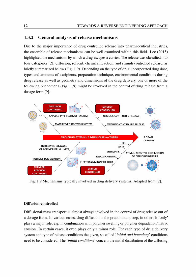
1.3.2 General analysis of release mechanisms
Due to the major importance of drug controlled release into pharmaceutical industries,the ensemble of release mechanisms can be well examined within this field. Lee (2015)highlighted the mechanisms by which a drug escapes a carrier. The release was classified intofour categories [2]: diffusion, solvent, chemical reaction, and stimuli controlled release, asbriefly summarized below (Fig. 1.9). Depending on the type of drug, incorporated drug dose,types and amounts of excipients, preparation technique, environmental conditions duringdrug release as well as geometry and dimensions of the drug delivery, one or more of thefollowing phenomena (Fig. 1.9) might be involved in the control of drug release from adosage form [9].
Fig. 1.9 Mechanisms typically involved in drug delivery systems. Adapted from [2].
Diffusion-controlled
Diffusional mass transport is almost always involved in the control of drug release out ofa dosage form. In various cases, drug diffusion is the predominant step, in others it ’only’plays a major role, e.g. in combination with polymer swelling or polymer degradation/matrixerosion. In certain cases, it even plays only a minor role. For each type of drug deliverysystem and type of release conditions the given, so-called ’initial and boundary’ conditionsneed to be considered. The ’initial conditions’ concern the initial distribution of the diffusing

1.3 State-of-the-art of controlled release technologies 13
species in the system. The mathematical treatment is much simpler if this distributionis homogeneous. The ’boundary conditions’ concern the conditions for diffusion at theboundaries of the drug delivery system. If the device dimensions are constant with time(no significant swelling or dissolution/erosion), the boundaries are called ’stationary’. Incontrast, in case of time-dependent device dimensions, the boundary conditions are called’moving’. If the device swells significantly, the boundaries are moving outwards; if the systemdissolves/erodes significantly, they move inwards. In case of ’perfect sink conditions’ thedrug concentration in the surrounding bulk fluid can be considered negligible. Furthermore,if the release medium is well stirred, the liquid unstirred boundary layer surrounding thedevice is generally thin. If the mass transfer resistance within the drug delivery system fordrug diffusion is much higher than the mass transfer resistance in this liquid boundary layer,the latter can generally be neglected. [10]
Solvent-controlled
Solvent transport into a drug carrier can influence the drug release behavior from the carrier.The solvent-controlled release includes osmosis-controlled release and swelling-controlledrelease [61]. Osmosis-controlled release occurs in a carrier covered with a semi-permeablepolymeric membrane, through which water can flow from outside of the carrier (with alow drug concentration) to the drug-loaded core (with a high drug concentration). Thismechanism results in a zero-order release profile as long as a constant concentration gradientis maintained across the membrane [62]. When glassy hydrophilic polymeric systems areplaced in an aqueous solution including body fluids, water diffuses into the system. Thewater uptake results in the swelling of the polymeric particles followed by drug release(swelling-controlled release). The drug release rate is determined by the diffusion rate ofwater and the chain relaxation rate of polymers [63]. The swelling-controlled systems consistof polymeric materials with three dimensionally crosslinked network such as hydrogels,where the mesh size plays a central role in controlling the drug release behavior [64]. Theswelling-controlled systems may achieve a zero-order drug release depending on the initialdrug distribution in the system [65] or polymer composition [66].
Chemical reaction-controlled
Drug carriers comprising biodegradable polymers such as polyesters, polyamides, poly(aminoacids), and polysaccharides release drugs via hydrolytic and/or enzymatic degradation ofester, amide, and hydrazone bonds in their backbones [67–69] . Matrices made of polymerslike poly(lactic-co-glycolic acid) (PLGA), polylactic acid (PLA), and polycaprolactone

14 TOWARDS A REVERSE ENGINEERING APPROACH
(PCL) undergo bulk degradation, resulting in simultaneous degradation of entire matrices.On the other hand, those made of polyanhydrides and poly(orthoesters) tipically erodefrom the surface into the core (surface degradation) as the polymer degradation occursfaster than water diffusion into the matrix [70]. However, in a small dimension matrixlike nanoparticles, where the distance of water diffusion is short and the domain size ofcrystallization is restricted, the polymer degradation is substantially accelerated, and thesepolymers do not necessarily follow the typical surface erosion behavior but show a sign ofbullk degradation (constant particle size during polymer degradation) [71]. Drug releasekinetics is determined by the degradation rate of polymers, which depends on their molecularweight, end groups, monomer, composition, and crystallinity [72]. "Biodegradable polymericsystems are preferable, because they are disintigrated into compounds that are readilyremoved from the body without causing long-term side effects" [2]. From drug polymerconjugates, a drug is released from the carrier via hydrolytic or enzymatic cleavage ofthe linkage between the drug and the polymer. The rate of cleavage controls the drugrelease kinetics [73]. "Enzymatically cleavable drug-polymer conjugates may be used fortarget-specific drug delivery, if the enzyme is concentrated in target issues" [74].
Stimuli-controlled release
Responsive polymer materials can adapt to surrounding environments, regulate transport ofions and molecules, change wettability and adhesion of different species on external stimuli,or convert chemical and biochemical signals into optical, electrical, thermal and mechanicalsignals, and vice versa [2]. "These materials are playing an increasingly important part ina diverse range of applications, such as drug delivery, diagnostics, tissue engineering andsmart optical systems, as well as biosensors, microelectromechanical systems, coatings andtextiles" [6]. Drug release from stimuli-responsive nanocarriers is controlled by internal orexternal stimuli such as temperature, pH, ionic strength, sound, and electric or magneticfields [46]. As it is possible to localize the stimuli, these carriers have been explored fortarget-specific drug delivery [2]. pH-sensitive carriers have been developed for tumor-specificdrug delivery and to increase the contrast between intracellular and extracellular drug release[75]. In thermosensitive drug carriers, drug release is caused by temperature-induced phasetransition of the polymer [76]. Because of the complexity and interdependence of the topics,it is difficult to categorize the published articles. A global classification as shown in Fig.1.10 may be useful in understanding the wide domain of transformations (reversible andirreversible) of stimuli-responsive nanocarriers based on polymers, colloids and surfaces.

1.3State-of-the-artofcontrolled
releasetechnologies
15
Fig. 1.10 Stimuli-responsive nanostructures based on polymers, colloids and surfaces Taken from [6].
p~~':"!.~ ~-~~~ .. Compact ~
' globule J / ~ Phylieal gel Micelle
;:::::::=~ · -_ ·- ·_ · ~-~ illll A Thin film Collapled brush Homopol. mor brush w ~-~ 0 T Y a Crolslinked micelle / Y 1\ Ill 11\, t >lUl ~ ~~~edgel '): ... nanogel / eapsule
~-~ ~~
..(-,., J:' "-J'-L'Sf' r
• • • • • ... -=:::::~-~ Hybtid thin film 1 b<ush
Cro$$1inked ~
' ~-~ Membrane
Swollen membrane
Stimuli--siva 1 reversible changes
Hierarchical development 1 irraversibkl transformations
~ ~-~ ~\~ ~-~ ~~-"Î'I\'t' ~ ~
~
" ~ "7t~Ç" Cor~·shell "'Pickering
~ particle emulsion
~ ~
o·~! Core-crosslin/ ed collapsed
!.<shell par1ide shol .... particle
~- ~ Â
~-~ ~ "'!, y
?t\~ 2-levet tiybtid gel
Cor&-hybrid shell particle
Aggregate

16 TOWARDS A REVERSE ENGINEERING APPROACH
1.4 Current tools for prediction of controlled release
Mathematical modeling of drug delivery and predictability of drug release is a field ofsteadily increasing academic and industrial importance with an enormous future potential.Because of the noteworthy advances in information technology, the ’in-silico’ or ’ab-initio’optimization of novel delivery systems can be required to essentially enhance in precisionand effortlessness of utilization. Comparable to other fields (e.g., aeronautics and aviation),computer simulations are probably going to wind up plainly a necessary piece of futureinnovative work in pharmaceutical innovation. "It is just an issue of time when numericalprojects will be routinely used to help optimizing the plan of novel dosage products" [9].Considering the desired type of administration, drug dose to be incorporated and targeteddrug release profile, mathematical predictions will allow for good estimates of the requiredcomposition, geometry, dimensions and preparation procedure of the respective dosageforms.
In this way, one of the real main thrusts for the utilization of mathematical modeling indrug delivery is to spare time and to diminish costs: the quantity of required experimentaltests to build up as well as the optimization of a current drug delivery product can altogetherbe diminished. Moreover, the quantitative examination of the physical, chemical, andconceivably natural phenomena, which are associated with the control of drug release, offersanother central preferred standpoint: the basic understanding on the release mechanismscan be illustrated. "This knowledge is not only of academic interest, but a pre-requisitefor an efficient improvement of the safety of the new pharmaco-treatments (particularly forhighly potent drugs with narrow therapeutic windows)" [9]. Moreover, potential difficultiesexperienced during production can be significantly more productively addressed if the systemis not dealt as a ’black box’, but there is an intensive comprehension of how drug releaseis controlled. It is definitive to know which product properties are critical to give a desiredperformance.
As Siepmann (2008) reviewed, up to date, numerous mathematical theories have beendescribed in the literature [77–79, 64], but most of them still lack in accuracy and/or easinessof application. The pioneer of mathematical modeling of drug delivery is consireded to beProfessor Takeru Higuchi. In 1961, he published his famous equation allowing for a simpleand surprising description of drug release from an ointment base exhibiting a considerableinitial excess of dissolved drug within an inert matrix with film geometry [80, 81]. This wasthe beginning of the quantitative treatment of drug release from pharmaceutical dosage forms.Numerous models have been proposed since then, including ’empirical/semi-empirical’ aswell as ’mechanistic realistic theories’. In the first case, the mathematical treatment is (atleast partially) purely descriptive and not based on real physical, chemical and/or biological

1.5 Empirical and semi/empirical mathematical models 17
phemonena. Consequently, no or very limited insight into the underlying drug releasemechanisms can be gained. Furthermore, the predictive power of empirical/semi-empiricalmodels is often low [9]. This kind of models may for example be valuable if diverse types ofdrug release profiles are to be compared utilizing a particular parameter (e.g., a release rateconstant for experimental design). However, extraordinary alert must be paid if mechanisticconclusions are drawn or quantitative predictions made. An exception are approaches basedon artificial neural networks (ANNs), which can show good predictive power.
In contrast, mechanistic mathematical theories are based on real phenomena, such asdiffusion, dissolution, swelling, erosion, precipitation and/or degradation [82–88]. This typeof models allows for the determination of system-specific parameters that can offer deeperinsight into the underlying drug release mechanisms. For instance, the relative importanceof several processes that are involved (e.g., drug diffusion and polymer swelling) can beestimated. The dosage form is not treated as a ’black box’, but as a real drug delivery systemwhere the mechanisms of which can be understood [9]. For product development suchmechanistic realistic mathematical models consider the quantitative prediction of the impactsof formulation and manufacture parameters (e.g., the underlying tablet heigth and radius)on the subsequent release. Accordingly, the required composition, size, shape and manufac-ture procedure of a novel dose frame with wanted properties turn out to be hypotheticallypredictable. In addition, challenges experienced during production are substantially lessdemanding to address while having a reasonable thought of how the system functions.
1.5 Empirical and semi/empirical mathematical models
1.5.1 Peppas equation
A very frequently used and easy-to-apply model to describe drug release is the so-calledPeppas equation, or power law [24]:
Mt
M∞
= ktn (1.1)
Here, Mt and M∞ are the absolute cumulative amount of drug released at time t and infinitetime, respectively; k is a constant incorporating structural and geometric characteristics of thesystem, and n is the release exponent, which might be indicative of the mechanism of drugrelease. Nicholas Peppas was the first to introduce this equation in the field of drug delivery[24]. A release exponent of 0.5 can serve as an indication for diffusion controlled drugrelease, but only if all assumptions these particular solutions are based on are fulfilled (filmgeometry with negligible edge effects, time- and position-independent diffusion coefficients

18 TOWARDS A REVERSE ENGINEERING APPROACH
Table 1.2 Release exponent n of the Peppas equation [24] and release mechanisms fromcontrolled delivery systems of different geometry. Taken from [9].
Drug release mechanismExponent, n
Thin film Cylinder Sphere
Fickian diffusion 0.5 0.43 0.43Anomalous transport 0.5<n<1.0 0.45<n<0.89 0.43<n<0.85Polymer swelling 1.0 0.89 0.85
in a non-swellable and insoluble matrix former) [9]. For other device geometries and puredrug diffusion control, different release exponent values have been derived [89, 90]. Incontrast, if polymer swelling is the solely release rate controlling mechanism and in thecase of a delivery system with film geometry, zero order drug release kinetics is observed,corresponding to a release exponent of n=1. But again, none of the model assumptions forthis particular must be violated. For other geometries than that of thin films with negligibleedge effects, different n-values can serve as indicators for purely swelling controlled drugdelivery (Table 1.2). Release exponents that are in between these extreme values for therespective device geometry indicate so-called ’anomalous’ transport, thus, an overlapping ofdifferent types of phenomena, potentially including drug diffusion and polymer swelling [9].
1.5.2 Hopfenberg model
Hopfenberg [91] proposed an interesting semi-empirical model allowing for a quantitativedescription of drug release from degradable drug delivery systems exhibiting a release whichis proportional to the (time-dependent) surface area of the device. All mass transfer processesthat are involved in the control of drug release are assumed to add up to a single zeroorder process (characterized by a rate constant, k0), which is confined to the surface area ofthe system. This zero order process might correspond to one single physical or chemicalphenomenon, but it might also result from the superposition of several processes, such asdissolution, swelling and/or polymer chain cleavage. The Hopfenberg model can for instancebe applied to surface eroding polymer matrices for which a zero order surface detachment ofthe drug is the rate limiting release step [9]. The general equation is as follows:
Mt
M∞
= 1−(
1− k0tc0a
)n
(1.2)
Here, Mt and M∞ are the cumulative absolute amounts of drug released at time t andat infinite time, respectively; c0 denotes the uniform initial drug concentration within the
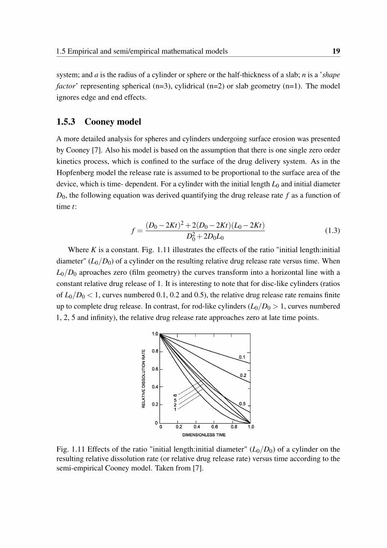
1.5 Empirical and semi/empirical mathematical models 19
system; and a is the radius of a cylinder or sphere or the half-thickness of a slab; n is a ’shapefactor’ representing spherical (n=3), cylidrical (n=2) or slab geometry (n=1). The modelignores edge and end effects.
1.5.3 Cooney model
A more detailed analysis for spheres and cylinders undergoing surface erosion was presentedby Cooney [7]. Also his model is based on the assumption that there is one single zero orderkinetics process, which is confined to the surface of the drug delivery system. As in theHopfenberg model the release rate is assumed to be proportional to the surface area of thedevice, which is time- dependent. For a cylinder with the initial length L0 and initial diameterD0, the following equation was derived quantifying the drug release rate f as a function oftime t:
f =(D0 −2Kt)2 +2(D0 −2Kt)(L0 −2Kt)
D20 +2D0L0
(1.3)
Where K is a constant. Fig. 1.11 illustrates the effects of the ratio "initial length:initialdiameter" (L0/D0) of a cylinder on the resulting relative drug release rate versus time. WhenL0/D0 aproaches zero (film geometry) the curves transform into a horizontal line with aconstant relative drug release of 1. It is interesting to note that for disc-like cylinders (ratiosof L0/D0 < 1, curves numbered 0.1, 0.2 and 0.5), the relative drug release rate remains finiteup to complete drug release. In contrast, for rod-like cylinders (L0/D0 > 1, curves numbered1, 2, 5 and infinity), the relative drug release rate approaches zero at late time points.
Fig. 1.11 Effects of the ratio "initial length:initial diameter" (L0/D0) of a cylinder on theresulting relative dissolution rate (or relative drug release rate) versus time according to thesemi-empirical Cooney model. Taken from [7].

20 TOWARDS A REVERSE ENGINEERING APPROACH
1.5.4 Artificial neural networks
Also artificial neural networks (ANNs) can be used to model drug delivery [8, 92]. The basicprinciple of this type of mathematical analysis is illustrated in Fig. 1.12. An ANN consistsof one input layer, one output layer and one or more hidden intermediate layers. Each layeris composed of several units, corresponding to ’neurons’. The input layer encompasses ninput values of causal factors, e.g. the drug loading, compression force or excipient content.The output layer can for instance consist of constants describing the drug release profile.As illustrated, the units of neighboring layers are interconnected, the links correspondingto ’synapses’. The strength of these links can vary, they are also called ’weights’. Upondefinition of the model structure a set of experimental results (consisting of input and outputvalues) is used to ’train’ the network, that is to define the optimal equations and weightsallowing for the calculation of the output values based on the input values. Thus, ANNs canbe considered as nonlinear regression analysis tools. Once the system is ’trained’, it canbe used to make quantitative predictions for the output values based on new input values.This type of analysis was used by Takahara [8] to simulate the effects of the amounts ofmicrocrystalline cellulose and hydroxypropyl methylcellulose as well as of the compressionpressure used to prepare trapidil-loaded matrix tablets on the resulting drug release kinetics.Ibric [93] applied ANNs to study acetylsalicylic acid release from Eudragit RS-based matrixtablets, whereas theophylline release from coated pellets was analyzed by Ghaffari [94] usingthis type of mathematical modeling approach. A further interesting application of neuralnetworks in drug delivery was presented by Shao [95], predicting drug release from andtablet tensile strength of immediate release formulations.
Fig. 1.12 Basic principle of mathematical modeling using artificial neural networks (ANNs):Xi represents the input value of causal factors, n is the number of causal factors, Yi denotesthe output value of responses and m the number of responses. Taken from [8].

1.6 Mechanistic realistic theories 21
1.6 Mechanistic realistic theories
1.6.1 Theories based on Fick’s law of diffusion
Diffusion-controlled drug release is typically shown in a capsule-type reservoir system, inwhich a drug is dissolved or dispersed in a core surrounded by a polymeric membrane [96].Drug diffusion is driven by the difference in its concentration across the membrane. Here,the drug first dissolves in the core, then diffuses through the membrane [9]. Matrix-typenanospheres, where drug molecules are dispersed throughout the polymer matrix, also showa diffusion-controlled release profile. In the matrix-type systems, there is no membrane thatserves as a diffusion barrier; therefore, this system usually shows high initial release, followedby a decreasing release rate with the increasing diffusion distance for drug molecules locatedinterior of the carrier [2]. In order to quantify diffusional mass transport, Fick’s laws ofdiffusion can be used [97]:
Fick’s first law of diffusion:F =−D · ∂c
∂x(1.4)
where F is the rate of transfer per unit area of section (flux); c is the concentration of thediffusing species and D denotes the diffusion coefficient (also called diffusivity).
Fick’s second law of diffusion (which can be derived from Fick’s first law and massbalance considerations):
∂c∂x
= D ·(
∂ 2c∂x2 +
∂ 2c∂y2 +
∂ 2c∂ z2
)(1.5)
where c is the concentration of the diffusing species; t denotes time, D is the diffusioncoefficient and x, y and z are the three spatial (Cartesian) coordinates.
A very important aspect when solving Fick’s second law of diffusion is the fact whetheror not the diffusion coefficient of the diffusing species is constant or not. The mathematicaltreatment is much simpler if D is constant. Reasons for time- and position- dependentdiffusion coefficient might include matrix erosion, polymer swelling and/or degradation.In these cases, generally no ’analytical solutions’ of Fick’s law can be derived (no ’exact’solutions quantifying the amount of drug released as a function of time), but ’numericalsolutions’ (’approximate’ solutions) can be used [9]. Notwithstanding, if drug release issimply diffusion controlled with constant diffusion coefficients, the numerical treatment canbe fairly direct. As Siepmann describes in his review [9] of mathematical modeling, differenttypes of systems can be distinguished (Fig. 1.13), including: (i) reservoir devices consistingof a drug depot, which is surrounded by a release rate controlling barrier membrane (often

22 TOWARDS A REVERSE ENGINEERING APPROACH
polymer-based), and (ii) monolithic systems, also called "one-block" systems, because thereis no local separation between a drug reservoir and a release rate controlling barrier.
Fig. 1.13 Classification system for primarily diffusion controlled drug delivery systems. Starsrepresent individual drug molecules, black circles drug crystals and/or amorphous aggregates.Only spherical dosage forms are illustrated, but the classification is applicable to any type ofgeometry. Taken from [9].
For both types of systems two subclasses can be distinguished: the initial drug concentra-tion is either below or above drug solubility in the device. In the case of a reservoir device(Fig. 1.14) with an initial drug concentration below drug solubility (e.g., a polymer-coatedtablet or pellet with a low drug loading), released drug molecules are not replaced andthe drug concentration at the inner membrane’s surface continuously decreases with time(non-constant activity source). If the membrane does not swell or dissolve, if perfect sinkconditions are provided throughout the release period and if the drug permeability throughthe barrier remains constant, first order release kinetics results, irrespective of the geometryof the device [98]:
∂Mt
∂ t=
ADKCt
l=
ADKl
· M0 −Mt
V(1.6)
Where Mt represents the absolute cumulative amount of drug released at time t; Ct
denotes the concentration of the drug in the release medium at time t; M0 is the initial amountof drug within the dosage form; V the volume of the drug reservoir, A the total surface areaof the device, and l the thickness of the membrane; K represents the partition coefficient of

1.6 Mechanistic realistic theories 23
the drug between the membrane and the reservoir, and D the diffusion coefficient of the drugwithin the membrane.
Fig. 1.14 Representations of reservoir devices (drug depot surrounded by a release ratecontrolling barrier membrane) at different geometries (slab, sphere, cylinder). Taken from[9]. Note that equations kinetics 1.6 and 1.7 are irrespective of the device geometry.
In contrast, if the initial drug concentration exceeds the drug solubility in a reservoir de-vice, released molecules are replaced by the (partial) dissolution of drug crystals/amorphousaggregates, resulting in constant drug concentrations (saturated solutions) at the inner mem-brane’s surface (constant activity source) [9]. If the properties of the release rate controllingbarrier (including its thickness and permeability for the drug) remain constant and if perfectsink conditions are provided throughout the release period, zero order release kinetics resultas long as drug excess is provided, irrespective of the geometry of the system [98]:
∂Mt
∂ t=
AJlim
l=
ADKCs
l(1.7)
where Mt is the amount of drug release at time t; δMt/δ t denotes the steady state releaserate at time t; A is the total surface area of the device, Jlim the membrane-limiting flux, l thethickness of the membrane, D the diffusion coefficient of the drug within the membrane,K the partition coefficient of the drug between the membrane and the reservoir, and Cs thesolubility of the drug in the reservoir. However, in practice often deviations from these ’ideal’systems are observed, for instance the film coatings show crack formation due to significanthydrostatic pressure built up within the device or due to membrane swelling and/or (partial)dissolution [99]. This renders the numerical treatment considerably more muddled and yetthere is a critical absence of mechanistic realistic mathematical theories considering thesefeatures.
In the case of monolithic devices, the system geometry significally affects the resultingdrug release kinetics. If the initial drug concentration is below drug solubility, the drugmolecules are individualized/dissolved within the carrier material (monolithic solution).Otherwise, dissolved drug molecules co-exist with amorphous aggregates and/or drug crystals(monolithic dispersions). In the case of monolithic solutions and in the absence of significant

24 TOWARDS A REVERSE ENGINEERING APPROACH
Fig. 1.15 Overview on the mathematical equations, which can be used to quantify drug releasefrom monolithic solutions (initial drug concentration<drug solubility). The "exact" equationsare valid during the entire release periods, the indicated early and late time approximationsare only valid during parts of the release periods. Taken from [10].
changes in the carrier matrix during drug release (e.g., constant porosity, no swelling,time-independent permeability for the drug) and if perfect sink conditions are maintainedthroughout the release period and if drug release is primarily controlled by diffusion throughthe carrier matrix, the resulting release can be calculated as showed in Fig. 1.15 , dependingon the system’s geometry [9].
Where Mt and M∞ denote the absolute cumulative amounts of drug released at time t andinfinity, respectively; n and p are dummy variables, D the diffusion coefficient of the drugwithin the matrix former, L (in the case of thin films with negligible edge effects [97]) is thethickness of the film, R (in the case of spherical dosage forms [97]) the radius of the sphere,(in the case of cylinders considering axial as well as radial mass transport [100] the radius ofthe cylinder, H denote the height of the cylinder and qn are the roots of the Bessel functionof the first kind of zero order [J0(gn) = 0]. To avoid the use of infinite series of exponentialfunctions, early and late time approximations have been proposed for these equations [98].
For monolithic dispersions (Fig. 1.16) the mathematical description becomes even morecomplex. For the simplest geometry of thin films with negligible edge effects, Takeru Higuchipublished the famous square root of time relationship between the amount of drug released
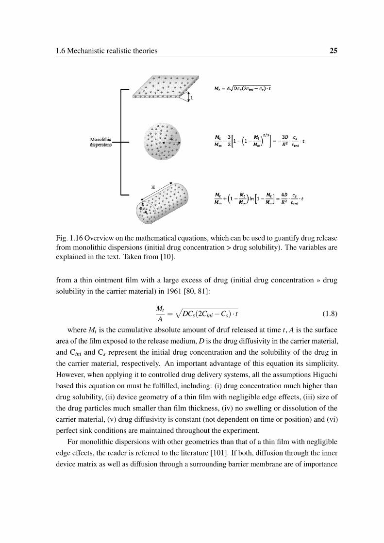
1.6 Mechanistic realistic theories 25
Fig. 1.16 Overview on the mathematical equations, which can be used to guantify drug releasefrom monolithic dispersions (initial drug concentration > drug solubility). The variables areexplained in the text. Taken from [10].
from a thin ointment film with a large excess of drug (initial drug concentration » drugsolubility in the carrier material) in 1961 [80, 81]:
Mt
A=√
DCs(2Cini −Cs) · t (1.8)
where Mt is the cumulative absolute amount of druf released at time t, A is the surfacearea of the film exposed to the release medium, D is the drug diffusivity in the carrier material,and Cini and Cs represent the initial drug concentration and the solubility of the drug inthe carrier material, respectively. An important advantage of this equation its simplicity.However, when applying it to controlled drug delivery systems, all the assumptions Higuchibased this equation on must be fulfilled, including: (i) drug concentration much higher thandrug solubility, (ii) device geometry of a thin film with negligible edge effects, (iii) size ofthe drug particles much smaller than film thickness, (iv) no swelling or dissolution of thecarrier material, (v) drug diffusivity is constant (not dependent on time or position) and (vi)perfect sink conditions are maintained throughout the experiment.
For monolithic dispersions with other geometries than that of a thin film with negligibleedge effects, the reader is referred to the literature [101]. If both, diffusion through the innerdevice matrix as well as diffusion through a surrounding barrier membrane are of importance

26 TOWARDS A REVERSE ENGINEERING APPROACH
for drug release (Fig. 1.13, ’miscellaneous’ systems), the mathematical modeling is alsomore complex and geometry dependent. Again, the reader is referred to the literature formore details [102].
1.6.2 Theories considering polymer swelling
If polymer swelling is of importance of the control of drug release, e.g. as in the case ofhydroxypropyl methylcellulose (HPMC)-based matrix tablets, the transition of the macro-molecules from the glassy (less mobile) to the rubbery (more mobile) state has to be con-sidered in the model [103]. The two most important consequences of significant polymersweeling in a controlled release matrix system are: (i) the length of the diffusion pathwaysincreases, resulting in decreasing drug concentration gradients (being the driving forces fordiffusion) and, thus, potentially decreasing drug release rates; (ii) the mobility of the macro-molecules significantly increases, resulting in increased drug mobility and, thus potentiallyincreasing drug release rates [9]. Fig. 1.17 schematically shows the physical phenomenawhich can be engaged with the control of drug release from a swellable delivery system.
Fig. 1.17 Schematic presentation of a swelling controlled drug delivery system containingdissolved and dispersed drug (stars and black circles, respectively), exhibiting the followingmoving boundaries: (i) an ’erosion front’, separating the bulk fluid from the delivery system;(ii) a ’diffusion front’, separating the swollen matrix containing dissolved drug only andthe swollen matrix containing dissolved and dispersed drug; and (iii) a ’swelling front’,separating the swollen and non-swollen matrix. Taken from [11].
This might represent a cross-section through half of a matrix tablet which is exposedto an aqueous bulk fluid in radial direction. On the right hand side, the inner tablet core isstill dry and in the glassy state (non-swollen), on the left hand side the bulk fluid is located.Upon contact with the release medium, water diffuses into the system. With increasingwater content, the mobility of the polymer chains (and, thus, also drug molecules) increases.

1.6 Mechanistic realistic theories 27
As soon as a certain, polymer-specific water concentration is reached, the macromolecu-lar mobility steeply increases. This phenomenon is called ’polymer chain relaxation’ or’glassy-to-rubbery-phase-transition’. The front at which this process takes place is called’swelling-front’, which separates the swollen from non-swollen matrix. Importantly, thisis not a stationary boundary but a moving one. The front that separates the swollen matrixcontaining only dissolved drug from the swollen matrix that contains both, dissolved andnon-dissolved drug, is called ’diffusion front’ (Fig. 1.17). Importantly also, this front ismoving. Furthermore, a third front can be distinguished, which separates the drug deliverysystem from the release medium and which is also moving. In the case of water-solublematrix formers, this front is called ’erosion front’ [9].
A very interesting example of mechanistic realistic mathematical theory allowing for thequantification of drug release from swellable polymer films has been proposed by Korsmeyeret al. [12]. It allows for a simultaneous consideration of the diffusion of water into the deviceand drug out of the system as well las of polymer swelling. To account for the increase inwater and drug mobility with increasing water content of the polymer matrix, a Fujita-typeexponential relationship was chosen [104] and shown to be appropriate for the prediction ofdifferent types of transport behaviors. Dimensional changes in the films are accounted for byallowing each spatial increment to expand according to the amount of water that diffusedin. At early time points, the swelling is restricted to one dimension by the glassy core of thesample. At later time points, when enough water has penetrated into the core of the systemto plasticize it, the sample relaxes to an isotropically swollen state. Afterwards, swelling isthree-dimensional. Under these conditions, water (subscript 1) diffusion can be described asfollows:
∂C1
∂τ=
∂
∂ξ·(
D1 ·∂C1
∂ξ
)(1.9)
where D1 is the diffusion coefficient of water, and C1 is the normalized water concentra-tion:
C1 =Cw
Cw,e(1.10)
Here, Cw is the water concentration in the film at a particular position, and Cw,e is theequilibrium water concentration in the system. Time t is scaled according to the waterdiffusivity in the fully swollen system, D1,s, and the dry thickness of the film, L0:
τ =tD1,s
L20
(1.11)

28 TOWARDS A REVERSE ENGINEERING APPROACH
The spatial coordinate x is normalized with respect to the dry thickness of the thin film:
ξ =x
L0(1.12)
To describe drug diffusion (subscript 2), the following equations are used:
∂C2
∂τ=
∂
∂ξ·(
D2 ·∂C2
∂ξ
)(1.13)
C2 =Cs
Cs,i(1.14)
Here, D2 is the diffusion coefficient of the drug, and C2 is the normalized drug concentra-tion; Cs denotes the drug concentration in the film, and Cs,i the initial drug concentration inthe system. The following boundary conditions are considered:
C1(0,τ) =C1(ξ ,τ) = 1 (1.15)
C2(0,τ) =C2(ξ ,τ) = 0 (1.16)
Where 0 and ξ are the two surfaces of the thin film. Please note that ξ describesthe continuously moving outside surface of the film. The following initial conditions areconsidered:
C1(ξ ,0) = 0 (1.17)
C2(ξ ,0) = 1 (1.18)
Due to the complexitiy of this set of partial differential equations, the latter was solvednumerically. As it can be seen in Fig. 1.18, good agreement between theory and experimentwas obtained when fitting this model to sets of experimentally measure theophylline releasekinetics from (hydroxyethyl methacrylate-co-N-vinyl-2-pyrrolidone) copolymer-based films.
1.6.3 Theories considering polymer swelling and drug dissolution
In practice, regularly considerably more more processes are simultaneously involved in thecontrol of drug release from oral controlled release matrix tablets. Generally, the matrixformer is water-soluble. Thus, also polymer dissolution must be taken into account [9].Different comprehensive mathematical theories have been proposed aiming to describe this

1.6 Mechanistic realistic theories 29
Fig. 1.18 Fit of the Korsmeyer-Peppas model to experimentally determined theophyllinerelease kinetics from hydroxyethyl methacrylate-co-N-vinyl-2-pyrrolidone copolymers-basedfilms (curve = theory, symbols = experiment). Taken from [12].
type of drug delivery systems [105, 77]. In the following, only one example will brieflybe described. The reader is referred to the literature for more details [105, 77]. The so-called ’sequential layer model’ [106] takes into account the diffusion of water and drug withtime- and position- dependent diffusivities, moving boundary conditions, the swelling of thesystem, polymer and drug dissolution, and radial and axial mass transfer within cylindricaltablets. The model was successfully fitted to drug release kinetics from matrices based onhydroxypropyl methylcellulose (HPMC) and HPMC derivatives.
Because the polymer dissolution must be taken into account, the complexity of partialdifferential equations increases, and numerical solution is required. Water and drug diffusionare considered based on Fick’s second law of diffusion for cylindrical geometry, taking intoaccount axial and radial mass transport and concentration-dependent diffusivities [97]:
∂Ck
∂ t=
1r
∂
∂ r·(
rDk ·∂Ck
∂ r
)+
∂
∂θ·(
Dk
r· ∂Ck
∂θ
)+
∂
∂ z·(
rDk ·∂Ck
∂ z
)(1.19)
Here, Ck and Dk are the concentration and diffusion coefficient of the diffusing species(k = 1 for water, k = 2 for the drug), respectively; r denotes the radial coordinate, z is theaxial coordinate, θ is the angular coordinate (Fig. 1.19a), and t represents time. Analogousto the Korsmeyer-Peppas model described above, a Fujita-type [104] exponential dependenceof the water and drug diffusion coefficients on the water content of the system is taken intoaccount:

30 TOWARDS A REVERSE ENGINEERING APPROACH
Dk = Dkcrit · exp−βk ·
(1− C1
C1crit
)(1.20)
where β1 and β2 are dimensionless constants characterizing this concentration-dependence.Also D1crit and D2crit denote the diffusion coefficients of water and drug at the interfacetablet/release medium, where polymer chain disentaglements occurs [105]. Ideal mixing isassumed (no volume contraction upon mixing drug, polymer and water), and the total volumeof the system at any time point is given by the sum of the volumes of the single components.The calculation of the new tablet dimensions is based on a mass balance considering drug,polymer and water. Polymer dissolution is taken into account using the reptation theory[107]: Above a certain critical water concentration (C1crit), the polymer chains at the surfaceof the tablet start to disentagle and diffuse through the liquid, unstirred layer surrounding thedevice into the bulk fluid (release medium). A dissolution rate constant, kdiss, is consideredcharacterizing the polymer mass loss velocity, which is normalized to the actual surface areaof the system:
Mpt = Mp0 − kdissAtt (1.21)
Here, Mpt and Mp0 are the dry polymer matrix mass at time t, and t = 0, respectively; At
denotes the surface area of the device at time t. The initial conditions reflect the fact that thematrix is dry and the drug uniformly distributed throughout the device at t = 0. The boundaryconditions are defined as follows: The water concentration at the surface of the matrix, C1crit
is calculated from the critical polymer disentaglement concentration. The drug concentrationat the surface of the tablet is assumed to be equal to zero (perfect sink condition). In orderto reduce computation time, the origin of the coordinate system is placed at the center ofthe cylinder, resulting in two symmetry planes for the drug and water concentration profiles(Fig. 1.19 b). Thus, only the concentration profiles within a quarter of the tablet need to becalculated. Due to the complexity of the resulting set of partial equations, also in this case anumerical solution is required.
Fig. 1.20 shows an example for a practical application of this mathematical model: Thetheoretically predicted effects of the initial radius of HPMC-based matrix tablets (with aninitial height of 2.6 mm, composition: 50% drug and 50% HPMC) on the resulting relativeand absolute release of theophylline into phosphate buffer pH 7.4 is illustrated. The curvesshow the theoretically predicted drug release profiles. Then, in a second step, the respectivedrug release rates were determined experimentally (symbols in Fig. 1.20). As it can be seen,good agreement between theory and experiment was obtained in all cases.

1.6 Mechanistic realistic theories 31
Fig. 1.19 Mathematical modeling of drug release from HPMC-based matrix tablets: (a)scheme of a cylindrical tablet for mathematical analysis, with (b) symmetry planes in axialand radial direction for the water and drug concentration profiles (Rt and Zt represent thetime dependent radius and half-height of the cylinder, respectively. Taken from [9].
1.6.4 Theories considering polymer erosion/degradation
Polymer degradation is the chain scission process by which polymer chains are cleaved intooligomers and monomers. In contrast, erosion is defined as the process of material lossfrom the polymer bulk. Such materials may be monomers, oligomers, parts of the polymerbackbone or even parts of the polymer bulk. Thus, the degradation of water-insolublepolymers is part of their erosion process [9]. Dependind on the relative rates of waterpeneteration into such systems and of polymer chain cleavage, two extreme types of erosioncan be distinguished: surface (or heterogeneous) erosion and bulk (or homogeneous) erosion.In the first case, the polymer chain cleavage is much faster than the water penetration into thesystem. Consequently, the degradation process is mostly restricted to the outermost polymerlayers and the erosion predominantly affects the surface, and not the inner parts of the device.In contrast, if water penetration is much more rapid than polymer chain cleavage, the entiresystem is rapidly wetted and degradation occurs throughout the device (bulk erosion) [61].Generally, drug delivery systems which are based on polymers with highly reactive bonds(e.g. polyanhydrides) in their backbone structure undergo surface erosion, whereas devicesthat are based on polymers with less reactive functional groups [e.g., poly(lactic-co-glycolicacid)(PLGA)] tend to be bulk eroding" [9].
An interesting mathematical theory for surface eroding drug delivery systems with filmgeometry was proposed by Lee in 1980 [13]. It is an analytical solution that is valid fordifferent ’drug loading:drug solubulity’ ratios. As illustrated in Fig. 1.21 a, the movementsof two fronts are considered: a diffusion front, and an erosion front. Here, R denotes thetime-dependent position of the diffusion front, and S the time-dependent position of theerosion front; A is the initial drug concentration within the delivery system, which is abovedrug solubility, Cs (monolithic dispersion); Cb represents the drug concentration in the well

32 TOWARDS A REVERSE ENGINEERING APPROACH
Fig. 1.20 Practical application of the ’sequential layer model’: Theoretically predicted effectsof the initial tablet radius on the release patterns of theophylline from HPMC-based matrixtablets in phosphate buffer pH 7.4 and experimental verification: (a) relative amount of drugreleased and (b) absolute amount of drug released versus time (37C), initial tablet height =2.6 mm, initial tablet radius indicated in the figures, 50% (w/w) initial drug loading) (curves:predicted values, symbols: independent experimental data). Taken from [9].
stirred release medium, and x the position (with x = 0 at the center and x = a at the surface ofthe film). It is assumed that the erosion front moves at a constant velocity, that edge effectsare negligible and that perfect sink conditions are maintained throughout the experiment.Under these conditions, Lee derived the following equations for a quantitative description ofdrug release:
Mt
M∞
= δ + τBaD
−δCs
A·(
12+
a3
6
)(1.22)
a3 =ACs
+δh−
√(ACs
+δh)2
−1−2δh (1.23)
h =12· Ba
D·(
1− ACs
)(1.24)
Here, Mt and M∞ are the cumulative absolute amounts of drug released at time t andat infinite time, respectively; δ denotes the relative separation between the diffusion anderosion fronts [δ = (S−R)/a]; B is the surface erosion rate constant with the dimensionsof a velocity; a represents the half-thickness of the film, D the drug diffusivity within thesystem, and τ is the dimensionless time (τ = Dt/a2). The parameter Ba/D is a measure forthe relative contribution of erosion and diffusion to drug release. The calculated effects on the’initial drug loading:drug solubility’ ratio (A : Cs) on the resulting drug release patterns areillustrated in Fig. 1.21 b. In this example, the relative contributions of erosion and diffusionare kept constant (= 1). As it can be seen, the relative drug release rate decreases with

1.6 Mechanistic realistic theories 33
Fig. 1.21 Modeling drug release from surface eroding monolithic dispersions with filmgeometry: (a) scheme of the drug concentration profile within the system according toLee (1980). Two moving fronts are considered: a diffusion front and an erosion front. (b)Calculated drug release profiles as a function of the ’initial drug loading:drug solubility’ratio (A/Cs).The parameter Ba/D serves as a measure for the relative contribution of erosionand diffusion. Taken from [13].
increasing A/Cs ratio. The model predicts that the release approaches zero order kineticswhen the initial drug loading becomes much higher than drug solubility in the matrix.
As polymer chain cleavage is a random process, Monte Carlo simulations can effectivelybe used to simulate polymer degradation. Zygourakis [108] was the first to propose thistype of theories allowing for a quantitative description of drug release from surface erodingpolymer matrices. The basic idea is to represent polymer matrix cross-sections by two-dimensional grids. Each pixel represents one of the system’s components: drug, polymerand potentially filler and pores. To simulate drug or polymer ’dissolution’ a so-called ’lifeexpectancy’ is defined for each type of pixel. As soon as a pixel comes into contact withwater, its ’lifetime’ starts to decrease. Once the ’lifetime’ expires, the pixel is assumed to’dissolve’ instantaneously. Importantly, different ’life expectancies’ can be defined for theinvolved system compounds, taking into account differences in their dissolution rates [14].
As example, an approach combining Monte Carlo simulations with diffusional transportwas used to quantify drug release from spherical poly(lactic-co-glycolic acid) (PLGA)-basedmicroparticles [109]. For the mathematical analysis, the latter are divided into concentricrings of equal volume (Fig. 1.22, the rings are described upon rotation of the pixels shown inFig. 1.22 b around the z-axis). Due to the symmetry planes at the r = 0 and z = 0 planes (inthe case of homogeneous initial drug and polymer distribution), it is sufficient to calculatethe mass transport phenomena in only one quarter of the two-dimensional circle shown in

34 TOWARDS A REVERSE ENGINEERING APPROACH
Fig. 1.22 Schematic presentation of a spherical PLGA-based microparticle for mathematicalanalysis: (a) three-dimensional geometry; (b) two-dimensional cross-section with two-dimensional pixel grid. Upon rotation of the latter around the z-axis, rings of identicalvolume are described. Taken from [14].
figures 1.22 b and 1.23 a. At t = 0 each ring represents either drug or non-degraded polymer.Due to the identical volume of the polymer rings it is reasonable to assume that each of themcontains a similar number of cleavable ester bonds. Thus, the probability with which a ringrepresenting non-degraded polymer degrades upon its first contact with water is similar forall rings. As described above, life time expectancies are assigned to all polymer pixels (rings),reflecting the degradation rate of the macromolecules. Importantly, knowing the status ofeach pixel (ring) (’non-eroded polymer’ or ’pore’) at each time point, the microparticleporosities in radial and axial direction (depending on time and position) can be calculated(Fig. 1.23 b). Based on these porosity values, the position- and direction-dependent drugdiffusivities within the spheres can be calculated as a function of the exposure time to therelease medium. This information is essential for the accurate calculation of the diffusionalmass transport processes using Fick’s second law [97].
∂C∂ t
=1r
∂
∂ r·(
rD · ∂C∂ r
)+
∂
∂θ·(
Dr· ∂C
∂θ
)+
∂
∂ z·(
rD · ∂C∂ z
)(1.25)
Here, c and D are the concentration and diffusion coefficient of the drug; r denotes theradial coordinate, z the axial coordinate, and θ the angle perpendicular to the r-z-plane. Inaddition, the limited solubility of the drug within the system is taken into account: Onlydrug which is soluble under the given conditions is considered to be available for diffusion.Taking into account the given initial and boundary conditions (initial homogeneous drugdistribution and perfect sink conditions), the set of partial differential equations is solvednumerically, using finite differences. Based on these calculations, system-specific parameterscan be determined and the dominant physical and chemical phenomena in each of the release

1.6 Mechanistic realistic theories 35
Fig. 1.23 Principle of a Monte Carlo-based approach to simulate polymer degradation anddiffusional drug release from PLGA-based microparticles. Schematic structure of the system(one quarter of the two-dimensional grid shown in Fig. 1.22b: (a) at time t=0 (before exposureto the release medium) and (b) during drug release. Gray, dotted and white pixels representnon-degraded polymer, drug and pores, respectively. Taken from [14].
periods be identified. For instance, it can be shown that this specific system the initial ’burstrelease’ is primarily controlled by pure drug diffusion. Furthermore, the model allows forquantitative predictions of the effects of formulation and processing parameters, includingthe initial microparticle size and drug loading. Importantly, good agreement between theoryand experiment was obtained (Fig. 1.24).
Fig. 1.24 Fit of a mechanistic realistic mathematical theory based on Monte Carlo simulationsand considering diffusional mass transport as well as limited local drug solubility to experi-mentally determined drug release from 5-fluouracil-loaded, PLGA-based microparticles inphosphate buffer pH 7.4: experimental results (symbols) and fitted theory (curve). Takenfrom [14].

36 TOWARDS A REVERSE ENGINEERING APPROACH
1.7 A reverse engineering methodology
1.7.1 Motivation
The research brings together chemists, physicists, and biologists. A lot of effort has beenmade to develop an ’ideal’ carrier. This promising scientific field is one of the fastest growing.However, it is unlikely that there will be one general theory that is applicable to any typeof delivery system. It is much more likely that there will be a broad spectrum of differentmathematical models, applicable to specific types of devices differing in geometry, activeingredient and excipient type. The literature on the subject of mathematical modeling isenormous and therefore difficult to distill into some globally useful steps. Cause of thisproblematic issue, one of the main concerns nowadays is the need for a systematic approachto controlled release product design, but also for efficient and reliable strategies to manage theassociated complexities, such as multidisciplinary problem, multiscale models, multicriteriaoptimization, multiple source of data and many more.
The process of obtaining useful higher-level representations of systems is called reverseengineering (RE), and remains a complex but very valuable goal to achieve. The applicationof RE principles and techniques in order to generate relevant model-based views of systems,facilitates their understanding and manipulation. In this context, the application of REmetholodogies [30] is practically used in order to (1) discover initial models from elementscomposing a given system and (2) understand (process) these models to generate relevantviews (i.e., derived models) on this system. However, generic and extensible solutionspotentially addressing several kinds of scenarios relying on different technologies are stillmissing or incomplete. Clearly, given that RE is a time-consuming and error-prone process,any RE solution that could (semi)automate the process would bring precious help to theusers, and thus facilitate its larger adoption.
This thesis proposes to make a step in the direction. The paradigm is largely based on theassumption that ’Everything is a model’ [110]. A whole model which defines the possibleelement types and structure of the systems which conform to it, similarly to the relationshipbetween a grammar and corresponding programs in the programming field. By means of anintegrated-modeling approach [111], the design problem is decomposed into a hierarchicalsequence of subproblems (boxes), combining computer-aided techniques with heuristic-based experimental testing. For a specific structured system, the idea is to implement theelements, concerning mass transfer, thermodynamics, formulation process, etc. which willallow afterwards to optimize an objective function (related to release rate) in order to choosethe best material (and features) for the best suited application. Thousands of alternatives(specific reverse engineering solutions) can be generated systematically and efficiently by

1.7 A reverse engineering methodology 37
this approach. Expressed as a reverse design problem, the target property for the productbecomes the known variable, and therefore, input for the design. This approach is the mostconvenient, because time and resources could be saved (compared to a simple experimentbased trial-and-error approach) and more realiable results can be obtained. In addition, thecombination of all these ’tools’ is useful for analyzing different scenarios including any kindof possible modification on systems.
1.7.2 A proposed reverse engineering framework
At the architecture level, the following framework (Fig. 1.25) is proposed.
Fig. 1.25 Work-flow diagram for a reverse engineering approach to help on the design ofcontrolled release products.
• Application domain, active ingredient and other components; The first boxes (1and 2) focuse on the definition of the target product profile, what do we want to do andwhy. The truth is that it is the area of interest and the question being asked that willdrive the metholodogy for modeling a particular system. This leads to the definitionof the critical design features for the product bearing in mind the route, frequencyof administration, safety or environmental considerations, as well as possibilities ofsecondary components included with the active ingredient in the mixture. For instance,

38 TOWARDS A REVERSE ENGINEERING APPROACH
pharmaceutical products or drugs, apart from the active principle include excipients,solvents, etc; in food industry, products have additives so that the products last longer;in cosmetics, body creams require a proper thickness which is usually related to lotionsefficiency, stability and its aceptability by the consumer with the proper absorption rateon the skin, etc.
• Thermodynamics and phase equilibria; Next, a reliable knowledge of the phaseequilibrium behavior of the systems is required to be designed (boxes 3 and 4). Duringthe last years, powerful thermodynamics models have been developed, which allow thecalculation of the various phase equilibria of multicomponent systems. For example,group-contributions models [112] such as UNIFAC are of major interest for a computer-aided design/verification based on ’define target - match target’. In the absence ofexperimental information of the mixture of interest, these models can be helpful forvisualizing trends and screening of potential product candidates; the search space foralternatives can be reduced and only few product candidates can be verified against thetarget or best performing ingredients.
• Formulation processing to obtain a dispersed system with specific parameters;Boxes 5,6 and 7 concern the formulation processing of the mixture from the basicingredients to the final product. A number of chemical and physical transformations areinvolved depending on the final dispersed system. Experimental testing will be helpfulto test limits and feasibility of the manufacturing procedures. In addition, the neededsystem parameters for the following theoretical simulations will be evaluated andidentified properly. As example of these parameters, the loading and concentration ofactive ingredient, the viscosity of the system, diffusion coefficients, phase geometries,or permeabilities through interface layers depending on thickness can be mentioned.
• Theoretical modeling and mathematical simulation Subsequently, boxes 8 and 9refer to mathematical models, mechanistic realistic approaches, special correlationsor numerical procedures that will be used for the target property estimation (releaserate). Attention will be focused on the assessment of the mass transfer occurring inthe inside/interface/outside areas of the dispersed system. Depending on the system,adapted boundary conditions as well as approaches based on one dimension or more(if necessary) could be employed.
• Experimental performance; Finally, the experimental resources (box 10) are appliedonly to test the likely best solutions and to verify or improve the former simulations.

Chapter 2
MODELING
’Everything should be as simple as possible, but not simpler’, Einstein
2.1 Introduction
A development of physicochemical models is fundamentally required to quantify masstransfer as function of product composition, structural parameters and active ingredientrelease processes. It is important bring to mind that modeling is an iterative process andsome models can take years before they become reasonably accurate. However, it is a helpfulhint to start with the simplest system (even if it highly unrealistic). Then, incrementally (insmall steps) add missing pieces and study the new system, comparing it to the data. With thechoice of a simple system, it is possible to get quickly initial models representing the basicparts. These ’raw’ models can be sufficiently accurate to be used as a starting point of otherscenarios. Eventually, in the reverse engineering framework, a subsequent increase on theabstraction or detail levels (boxes) would lead to bridge the gap between different proposedsolutions for controlled delivery. These more ’processed’ models obtained at the end, couldbe then finally used to generate and/or display the expected views of the framework in a widerange of structured products.
At the present chapter, the main purpose is to arrive at a model conception for the masstransfer in a system model without adjustable parameters by choosing different approachesfrom the literature. It is the purpose of this thesis to focus only into the most ’fundamental’and ’simple ones’. A brief description of the different theoretical approaches will be presented.On the basis of these models, a set of different simulation tools will be developed later ina next chapter, in order to fill out the different pieces (boxes) of the reverse engineeringframework previously proposed, and ultimately building a complete ’ab-initio’ model.

40 MODELING
2.1.1 Choice of a system model for ab-initio modeling
Emusion technology is particularly suited for design and fabrication of delivery systems[113]. Traditionally, conventional emulsions consisiting of small spherical droplets of oneliquid dispersed in another immiscible liquid, are used in industrial and medical applicationsfor a variety of reasons: encapsulation and delivery of active components; modificationof rheological properties; alteration of optical properties; lubrication; or modification oforganoleptic attributes (among others). The two immiscible liquids are typically an oilphase and an aqueous phase, although other immiscible liquids can sometimes be used. Thedroplets in conventional emulsions usually have diameters in the range of 100 nm to 100 µm,and are coated by a single layer of active surface components (’emulsifiers’) that stabilizethem against aggregation. For designing conventional emulsions, there are a limited numberof ways (Fig. 2.1) that droplets can be designed to provide specifical functional properties,such as stability, rheology, lubricity, optical properties, encapsulation, and delivery [15].
Fig. 2.1 Droplet, interfacial and phase characteristics that can be systematically altered tocreate building blocks of emulsions with different properties. Adapted from [15].
The major advantage of using the conventional emulsion design approach to createfunctional properties in emulsions is that they are relatively straightforward and inexpensiveto implement, which is important for many industrial applications. On the other hand,

2.1 Introduction 41
during the past decade, there have been major advances in the utilization of structural designprinciples to fabricate emulsions with novel functional properties and enhanced functionality[15], such as layering (tailor made coatings around the particles), clustering (control of theaggregation state of the droplets) and embedding (comprising droplets within larger particlesof a different material). These novel approaches allow to create functional attributes thatcannot be achieved using conventional emulsions (See Fig. 2.2).
Since that these emulsion-based delivery systems can potentially depict an increasingnumber of scenarios depending on different levels of complexity, it is forecasted that they willoffer an interesting framework of possibilities in order to implement a reverse engineering.
Fig. 2.2 Examples of structured emulsions that can be created by structural design principlesusing emulsion droplets as a building block.
Because of the enormous ’know-how’ developed in our laboratory during the last years,regarding the preparation of highly concentrated emulsions (thesis of Emilio Paruta, 2010)and also mass transfer within these systems (thesis of Hala Fersadou, 2011), we considerthat they are presented as a relevant model system for the start-up of the reverse engineeringthat this thesis proposes.
Highly concentrated emulsions allow a high amount of dispersed phase, and a high abilityto encapsulate active substances. As conventional emulsions, they can be of the oil-in-water(O/W) or water-in-oil (W/O) type. The different polarities of domains enable to solubilizehydrophilic and/or lipophilic molecules. Even though identified along as complex systems,these emulsions are very flexible regarding composition, size distribution, phase equilibria,interface type, morphology and viscosity. Therefore, they gather very good features to beapplied a reverse engineering and to perform experimental validations.
A characteristic feature of these emulsions is their gel-like texture, leading to a significantimprovement of emulsion stability, and offering a wide range of possibilities cocerningrheological properties and droplet size diameter. By way of illustration, in the followingpages, a publication concerning the effects of formulation and processing on the rheologicalproperties of oil-in-water highly concentrated emulsions is shown.

Contents lists available at ScienceDirect
Colloids and Surfaces A
journal homepage: www.elsevier.com/locate/colsurfa
Hydrophobically modified dextrans as stabilizers for O/W highlyconcentrated emulsions. Comparison with commercial non-ionic polymericstabilizers
Antonio Aguilera-Miguela,b, Edeluc López-Gonzaleza,b, Véronique Sadtlera,b,⁎, Alain Durandc,d,⁎⁎,Philippe Marchala,b, Christophe Castela,b, Lionel Choplina,b
aUniversité de Lorraine, LRGP, UMR 7274, Nancy F-54001, Franceb CNRS, LRGP, UMR 7274, Nancy F-54001, FrancecUniversité de Lorraine, LCPM, UMR 7375, Nancy F-54001, Franced CNRS, LCPM, UMR 7375, Nancy F-54001, France
G R A P H I C A L A B S T R A C T
A R T I C L E I N F O
Keywords:Non-ionic polymeric stabilizerHighly concentrated emulsionEmulsion rheologyLong-term stability
A B S T R A C T
Two amphiphilic polysaccharides derived from a nonionic bacterial polysaccharide of dextran (DexP10 andDexP15) have been explored as emulsifiers for preparing highly concentrated oil-in-water emulsions in a semi-batch (two-step) process. A fixed amount of stabilizer (10 g/L of emulsion) was employed for preparing emul-sions at dispersed-phase volumetric fractions ranging from 0.850 to 0.938. Their performances as stabilizers(interfacial tension, kinetics, droplet size distribution, rheological behavior and stability) were evaluated andcompared with a group of four ABA non-ionic commercial stabilizers from Pluronic series (F68, F127, P105 andL64) and a low-molecular-weight surfactant (Tween 80). Our results demonstrate these ABn graft amphiphilicpolysaccharides can be promising stabilizers as efficient as commercial non-ionic polymeric stabilizers forpreparing highly concentrated emulsions in spite of lower interfacial tensions, slower kinetics, or showingemulsions a larger droplet size and less monodispersity.
https://doi.org/10.1016/j.colsurfa.2018.04.022Received 13 February 2018; Received in revised form 9 April 2018; Accepted 10 April 2018
⁎ Corresponding author at: Université de Lorraine, LRGP, UMR 7274, Nancy F-54001, France.⁎⁎ Corresponding author at: Université de Lorraine, LCPM, UMR 7375, Nancy F-54001, France.E-mail addresses: [email protected] (V. Sadtler), [email protected] (A. Durand).
Colloids and Surfaces A 550 (2018) 155–166
Available online 12 April 20180927-7757/ © 2018 Elsevier B.V. All rights reserved.
ELSEVIER
ABngraft 2250
§" 225 247 glucose 2000 AB"-graft
i 200 ~DexP, 5 175
1750 - *-" DexP,0
ill "' ABA-block 0 150
Q:. 1500 g ABA ----- F68
~ 125 black '-' 1250 -.- F127
100 EO "' -<>- L64 ~
0 100 3 1000 --<>- P105 !0!
., 0 LMW
tl 75 u- ::;; 750
black ~ ~Tween80 0 50 "' iii
. . .. Ü.ow LMW fil 500
~ 25 20 EO ë:
...... ~ .. \" 250
o. e ~ o 0 ~ 65 PO 56 PO 37Phe 30PO 27 Phe sorbitan /ole11te I
6 0,64 0,85 0,86 0,87 0,68 0,89 0,90 0,91 0.92 0,93 0.94 • " 0 x *
F127 P105 DexP15
L64 F68 De x P 10
Tween 80 Dispersed-phase volumetrie fraction f (adim.]

1. Introduction
Highly concentrated or High-internal-phase-ratio (H.I.P.R.) emul-sions [22], also called gel-emulsions [35] or hydrocarbon gels [41],have many interesting applications within agrochemicals, pharmaceu-ticals, and personal care products. These emulsions have an extremelyhigh content of dispersed phase volume fraction (ϕ). When ϕ is largerthan the maximum packing volume fraction (ϕ*) of about 0.74 (mostcompact arrangement of mono-disperse hard spheres [36], reached fora face-centered cubic packing), the drops are no longer present asspheres but are distorted into polyhedral shape. This structure gives riseto a number of peculiar and fascinating properties including highviscosities and viscoelastic rheological behavior [37].
The stability is one of the most important factor to consider inemulsions. An emulsion is stable when there is no change on the dropletsize distribution or the spatial arrangement of droplets over the ex-perimental time scale [17]. Currently, there is an increasing tendency tosubstitute molecular surfactants by macromolecular stabilizers to for-mulate emulsions because high molecular weight polymeric stabilizershave the advantage that their adsorption onto the droplet surface ismuch firmer than with low-molecular-weight surfactants. This occursbecause polymeric surfactants attach to the droplet surface via severalsegments. Furthermore, they provide a thick steric barrier againstflocculation and coalescence at the droplet surface, and consequently,they can be used in low concentrations and much more efficiently [28].The most effective stabilization of oil-in-water (O/W) emulsions isgenerally obtained using ABA block or ABn graft polymeric stabilizers[50].
Many polysaccharides are amphiphilic polymers that have extendedflexible structures [13]. They are particularly attractive because of theirgood water-solubility, low toxicity and low interaction with living or-ganisms. Some examples of ABn graft stabilizers can be prepared bychemical modification of dextran [43]. By changing the conditions ofthe reaction [44], the number of the hydrophobic groups grafted ontothe neutral polysaccharide chains can be controlled, giving rise to dif-ferent amphiphilic dextrans of ABn graft type, capable for emulsionstabilization. It has already been shown in the literature that amphi-philic polysaccharides can exhibit surface-active properties and to beefficient oil-in-water emulsion stabilizers for oil volume fractions up to50 %. Nevertheless, to the best of our knowledge, there are no pub-lished studies about their use in highly concentrated emulsions (ϕ ≥0.74).
This paper has two purposes. On one hand, we want to shine newlight on the use of these amphiphilic polysaccharide-based stabilizersfor preparing highly concentrated O/W emulsions. On the other hand,we compare their performances as emulsifiers with polymeric stabi-lizers, and low-molecular-weight surfactants. By using a fixed massamount of stabilizer (10 g/L of emulsion), and a two step semi-batchprocess, the effect of ϕ on droplet size distributions and storage moduliof the emulsions was examinated. The stability of emulsions producedwas also evaluated. Stabilizer concentrations were generally higherthan critical concentrations determined by tensiometry and criticalmicelle concentrations reported on literature. This range is still largelyunexplored in the literature, however is quite relevant for industrialapplications [33].
2. Materials and methods
2.1. Materials
2.1.1. Dispersed and continuous phasesThe dispersed phase was dodecane (Reagent Plus® 99%), obtained
from Sigma–Aldrich and used as received. The continuous phase waswater deionized and milli-Q filtrated by a Millipore apparatus.
2.1.2. Stabilizers
• ABn graft – amphiphilic polysaccharide stabilizers: Two examples ofphenoxy-hidrophobically modified dextrans (DexP10 and Dex15)were used. These stabilizers consist of a hydrophilic backbonewithin which hydrophobic units are randomly distributed (seeFig. 1a). They were synthesized as described in [44], by covalentattachment of hydrophobic groups (phenoxy groups) onto a poly-saccharide backbone of dextran T40. The substitution ratio ornumber of grafted hydrophobic groups (B) per 100 glucopyranoseunits (A) was 10 and 15 respectively. For comparison purposes, thebackbone can be considered as a linear chain length of an average of247 glucopyranose units (molecular weight of dextranT40= 40,000 g/mol).
• ABA block – polymeric stabilizers: Four surfactants from thePluronic series F68, F127, P105 and L64, supplied by BASF(Germany) were used as received. These water soluble polymericstabilizers (see Fig. 1a) consist of two poly-A blocks chains of poly(ethylene oxide) (POE) and one B-block chain of poly (propyleneoxide) (PPO) [1]. They were chosen as most commonly reported onliterature and varying almost twice, three and four times the totalaverage molecular weight and also their hidrophobe/hidrophile partin different proportions.
• Low-molecular-weight (LMW) stabilizer: A polyethylene sorbitolester (Tween 80), supplied by Sigma–Aldrich was also included inthis study as example of commercial surfactant of relatively lowmolecular weight (see Fig. 1c).
Fig. 1. Typical molecular structures of stabilizers employed in this study.
A. Aguilera-Miguel et al. Colloids and Surfaces A 550 (2018) 155–166
156
A
OH
r= IOO · A (A+B)
r =Degree of hydrophobie substitution (%)
(a) ABn-graft amphiphilic polysaccharide : DexPr
(b) ABA-block polymerie stabilizer (Pluronic)
0
. 0. 1::1~H HOV"oHo~o~
w+x+y+z=20
(c) Low-molecular-weight (LMW) stabilizer: Tween 80

2.2. Methods
2.2.1. Interfacial tension measurementsA drop volume tensiometer (Tracker, IT Concept) was used to
measure the interfacial tension (γ) of a rising dodecane oil drop in so-lutions of aqueous stabilizer at 25 °C by analyzing the axisymmetricshape (Laplacian profile). The effect of the stabilizers on the interfacialtension was measured as function of the concentration. For an interfacedodecane – water the value of the initial interfacial tension was around50mN/m. A value of 0.1 for the Bond number was set as optimum toobtain an appropriate volume of droplet and to avoid escape effectsduring the measurement. It took hours or even a day for more dilutedsolutions to obtain a stationary interfacial tension. At this moment, arepresentative value with a 5% accuracy was taken.
2.2.2. Rheological measurementsThe rheological characterization of the prepared emulsions was
performed using a controlled stress rheometer AR-G2 (TA Instruments),equipped with a parallel plate geometry of smooth aluminum steelsurfaces of 40mm diameter. According to the literature [45], wall slipeffects clearly decrease as dispersed-phase and emulsifier concentra-tions increases in this kind of systems. In any case, no significant in-fluence by change of gap on the measurements was noticed.
Storage moduli (G′) values were determined via small amplitudeoscillatory-shear tests, into the linear viscoelastic domain of the sam-ples. Generally, it was observed for all samples that a strain of 0.1% atconstant frequency of 10 rad/s was enough to remain within the lineardomain. Scanning (sweep) shear rate measurements with a decreasingshear rate from 70 to 0.1 rad/s were carried out to get the characteristicviscoelastic parameter Plateau modulus, G°N [5]. This parameter, whichis considered as a measurement of the aggregation number of dropletscomprising the dispersed phase, is related to the droplet interactions
Table 1Properties of stabilizers employed in this study.
Stabilizer Chemical structurea MW HLBb γ CCc CMC
Tween 80 C14H34-COO–SR(EO)20 1310 14.5 6.63 35.3mg/L [55]; 57.6 mg/L [4]L64 (EO)13(PO)30(EO)13 2900 8 11.03 70 g/L [2]; 4.6 g/L (30 °C) [25]P105 (EO)37(PO)56(EO)37 6500 10 3.23 5.91 g/L in D2O [23]F68 (EO)76(PO)29(EO)76 8400 15.6 12.26 100 g/L [27]; 25 g/L [46]F127 (EO)100(PO)65(EO)100 12600 14 4.22 2.6 g/L [48]; 9 g/L [2]DexP10 H(C6H10O5)247(C9H11O3)25 43870 19 9.95 13.16 g/L [this work]DexP15 H(C6H10O5)247(C9H11O3)37 45800 18.6 11.77 10.076 g/L [this work]
a EO: ethylene oxide; PO: propylene oxide; SR: sorbitan ring; Oleate: C14H34eCOOe; phenoxy subunit: C9H11O3.b Calculated using the Beerbower and Hills equation [6] HLB=20×MH/(ML+MH) where MH and ML are the MW of hydrophilic and lipophilic portions of the
stabilizers. It is assumed EO and glucose (C6H10O5) as hydrophilic units.c γ CC = Interfacial tension [mN/m] for an interface dodecane – aqueous surfactant solution at C > CC.
Fig. 2. Structure of the compared stabilizers. The dot line represent an interfacewater/oil (W/O). For sake of clarity, the hydrophobically modified dextranshave been depicted vertically. The number and type of hydrophobic blocks foreach stabilizer are also specified on the x axis.
Fig. 3. Effect on interfacial tension (W/O interface) as function of stabilizerconcentration at 25 °C. Interfacial tension values at critical concentration (γ CC)are also shown.
Fig. 4. Viscosity of continuous phases prior emulsification. Each point re-presents the initial concentration of stabilizer in the continuous phase at a givenϕ (from left to right: 0.850; 0.900; 0.913; 0.930 and 0.938).
A. Aguilera-Miguel et al. Colloids and Surfaces A 550 (2018) 155–166
157
250 0,030 ASn graft ASn graft w 0
Ul 225 247 glucose 247 glucose AB,-graft =ê 'ii' 0,025 :J 200 ----*- DexP10 .0
ro :J
Cl. ----*"- DexP15 (/) 175 .s
Q) ~ O,Q20 (/) ABA-block 0 150 () ASA ro -- F127 :J
.<::
~ 125 block a. -- F68 (J) 0,015
0 100 EO ASA :J ----6--- P105
0
0 100
Lt:~0w block :J --+-- L64
~ c
76 EO ~ 0,01 0 LMW (/) 75 0
""" ASA () --~<---- Tween 80 () 0 50 block LMW 0 iii :f? 0,005 §l 25 13 EO 20 EO (J)
0 J:: ______ ?. .. ~ ()
a. 0
(J)
0 > 0,000 -o +------+ ~o - 0 ,. 65 PO 56 PO 37 Phe 30PO 29 PO 27 Phe sorbitan / eleate
I 60 80 100 120 140 160 • !;,. * <> • x * F127 P105 DexP
15 L64 F68 DexP
10 Tween 80 Stabilizer concentration in continuous phase C [g/L]
20 19 AB, -graf! Y cc [mN/m] 18 17
---*- DexP15
11 ,77
16 ----*- DexP10
9,95
'E 15
z 14
.s 13
;>-12
ABA-block ----- F68 12,26 -1t- L64 11 ,03 ----- F1 27 4,22
c 11 0 10 '(ii c 9 2 8
----6--- P1 05 3,23 LMW --~<---- Tween 80 6,63
cu 7 ·c:; 6 ~
2 5 c 4
3 2
0 5 10 15 20 25 30 35
Stabilizer concentration C [g/L]

and strength of the emulsion. The short-cut method proposed by Wu[54] was used to estimate G°N from the loss tangent (tan δ=G″/G′):
° = ′ →G G δ[ ] (tan )N minimum
The viscosity of continuous phases (prior emulsification) at differentϕ, were also measured by using a low shear viscosimeter LS300.
2.2.3. Determination of droplet size distributionsThe droplet size distributions (DSD) of the emulsions were obtained
using a Malvern Mastersizer 2000 (Malvern Instruments, U.K.). Abeaker containing 600mL of deionized and milli-Q filtrated water at astirring rate of 1000 rpm was used as dilution blank for all measure-ments. Refraction indexes of 1.330 and 1.419 were used for water anddodecane respectively. The standard percentile D0.5 (size in microns atwhich 50% of the sample is smaller and 50% is larger), was chosen asthe representative diameter for the emulsion samples. Optical ob-servations obtained by a BX51 Olympus microscope showed resultsfrom Mastersizer can be taken as the real droplet size distribution ofemulsions.
2.2.4. Preparation of highly concentrated emulsionsEmulsion volumes of 40mL were prepared in a simple two step
semi-batch process, similar as described in [3]. A brief description isgiven below:
1. Continuous phase preparation. A fixed amount of surfactant (0.4 g)was incorporated into every aqueous phase. Different volumes ofwater were used depending on the ϕ to prepare; ranging from 6mL(ϕ=0.850) to 2.5mL (ϕ=0.938). The mixtures were allowed forthermodynamic equilibration during 24 h prior to proceeding to thenext step.
2. Oil incorporation. The agitation turbine of a Turbo Test 33/750 P(Rayneri Groupe VMI), equipped with a 45° pitched agitator (4blades) of 35mm diameter, was positioned on the free surface of thecontinuous phase at a speed of 800 rpm. The oil phase was stepwiseadded to an emulsification vessel of 45 mm at a constant flow of17.2 mL/min by a peristaltic pump (BVP, Ismatec). The temperaturewas controlled at 25 °C with a Polystat 12HT thermostatic bath(Bioblock Scientific).
3. Homogenization. After the oil incorporation, emulsions were keptstirring using the same agitation turbine and vessel during 10 min at1000 rpm. This assured homogeneity of the dispersion. Emulsionsamples were taken one hour after processing to measure theirstorage moduli and obtain their droplet size distributions. The re-maining was transferred to a capped jar to prevent evaporation andwas kept at room temperature. Properties were measured along amaximum time scale of two years.
3. Results and discussion
3.1. Characteristics of stabilizers in aqueous solutions
Table 1 summarizes the properties of the stabilizers; such as che-mical structure, average molecular weight (MW), hydrophilic-lipophilicbalance (HLB), interfacial tension (γ CC) and critical micelle con-centration (CMC) values found in the literature. In Fig. 2 their struc-tures are depicted.
3.1.1. Interfacial tension measurementsStudies of adsorption of ABA-block polymeric surfactants at oil-
water interfaces are scarce [38,39,34]. Comparison with extensivestudies at air-water shows in general an analogous behavior at bothinterfaces [49]. We measured the effect on the interfacial tension (γ) ofthe stabilizers in aqueous solutions as function of the concentration.The results are plotted in Fig. 3. Generally, as the concentration ofstabilizer increased, a lowering in γ occurred until a critical
concentration (CC) above which no further decrease is observed. For allstabilizers, the CC values were found to be of the order of 1–10 g/L.These CC values are likely related to the formation layer at the inter-face, from which, further increases in the bulk concentration do notcause any more adsorption and as consequence, γ remains constant.Assuming that higher concentrations would not change this value, anaverage for γ using the last points (γ CC) has been taken to characterizeevery system.
The more hydrophobic ABA block stabilizers; P105 and F127, with56 and 65 PO units respectively, were the most effective on decreasingthe interfacial tension (until 3–4mN/m). As a general trend, longer POPblocks decrease interfacial tension to a larger extent because POP ismore surface active than POE [21]. This is clearly observed whencomparing these stabilizers with those of shorter POP blocks: L64 andF68, of 13 EO and 76 units respectively. Nonetheless, longer POE blockscan also result in a decrease of the interfacial tension because of anincreased repulsion between the POE chains [7]. This would explain thehigher reduction when using P105 instead of F127 or L64 instead ofF68 in spite of having a similar number of central POP blocks. Con-versely, the LMW stabilizer Tween 80, having a structure combining asingle hydrocarbon group (oleate) and a bulky non-ionic polar group(sorbitan ring), led to an intermediate value of 6.63mN/m. Surpris-ingly, the amphiphilic polysaccharides DexP10 and DexP15 with muchless hydrophobic nature (25–37 phenoxy subunits) decreased γ to asame extent (up to 11–12mN/m) than Pluronics L64 and F68. Possibleinteractions between the hydrophile glucose chains could also explainthe higher reduction when using the less substituted DexP10.
3.1.2. Concentration of stabilizerThe range of used concentrations at this work is shown in Fig. 4.
Every point represents the initial mass concentration of stabilizer in thecontinuous phase at different ϕ (from 0.850 to 0.938). These valuesrange from 60 to 180 g/L. In general, it is assumed that block copoly-mers and low-molecular-weight surfactants in a selective solvent formmicelles via a so-called closed association process, characterized by acertain CMC, below which only molecularly dissolved stabilizer ispresent in solution, usually as unimers [42]. On the other hand, am-phiphilic polysaccharides have shown that they can also behave likeclassical associative polymers [44]. Generally, it is assumed that at CMCand slightly above it, micelles are still loose but with further increase inamphiphile concentration in the medium, the unimer-micelle equili-brium shifts towards micelle formation [18]. Although the CMC is de-fined as a single concentration point, the micellization and micellestructure transitions can occur in a relatively broad range of con-centrations in the proximity of the CMC [51]. This implies micellesbecome more tight and stable and decrease their size during this tran-sition. It could be reasonable to think that previous CC determined bytensiometry should be related to those CMC reported on the literature(see Table 1). However, caution must be always applied because find-ings from different authors might not be transferable. In practice, acertain CMC range with some notable uncertainty could be detected,and large differences are often noted between CMC values determinedby different methods [1] because their sensitivity to quantity of mole-cularly dispersed unimers present may vary or because of the presenceof impurities. For any case, in this work, we assume and consider thatall concentrations employed at this work are generally higher thanthese both CC and CMC. Therefore, we hypothesize that the excess ofconcentration above the CC, will be turned into a higher amount ofmicelles with probably different shapes existing in the aqueous solu-tion.
3.1.3. Viscosity measurementsThe viscosities of the stabilizer solutions employed as continuous
phases at a given ϕ, were shown in Fig. 4. Identical or very closeviscosity values were found when using different stabilizers at differentconcentrations. All aqueous solutions showed a Newtonian flow
A. Aguilera-Miguel et al. Colloids and Surfaces A 550 (2018) 155–166
158

behavior with viscosities ranging in the order of a few times the visc-osity of water. The values increased with ϕ for every system. Generally,the higher the MW of the stabilizer, the higher the viscosity of theaqueous solution at a same ϕ. However, for Pluronic F127, it was ob-served that the viscosity was many times greater than all the others,specially at the highest ϕ. This finding reveals that the most importantdegree of interaction between the stabilizer molecules (micelles) withinthe continuous phase, likely occurs when this stabilizer is used.
3.2. Comparison of stabilizers
3.2.1. Effect of volumetric fraction (ϕ) on droplet size (D0.5)A set of DSD obtained at five ϕ by using the same semi-batch process
at fixed total stabilizer concentration of 10 g/L emulsion can be vi-sualized in Fig. 8. In general, the DSD of all emulsions evolve from aslightly polydispersed to a more ordered monodispersed system as ϕincreases. In Fig. 5 are shown plots of D0.5 versus ϕ. It was noticed alinear decreasing relation between D0.5 and ϕ for each stabilizer alongthe whole range of volumetric fractions studied. At a given ϕ, stabilizerswith lower γ produced emulsions with smaller droplet sizes. This in-dicates clearly that the droplet diameter depends on the interfacialtension. However, the tendency diminishes as ϕ increases. This is ex-plained because at high ϕ, it is the viscosity global of the emulsionwhich dominates the process of emulsification. This tendency corro-borates ideas from previous authors [9] who argued that when the oilcontent increases, it is the emulsion viscosity that controls droplet size,regardless of the dispersed-phase viscosity and hydrodynamics. As au-thors pointed out, this implies that the efficiency of the mixing processis strongly improved by increasing the internal phase content, and lesspower input is necessary for a more efficient droplet rupturing process.
However, it is interesting to note that no differences were foundconcerning D0.5 when employing Pluronic stabilizers F127 and L64,despite differences on viscosity of continuous phases, interfacial tensionand HLB, coinciding D0.5 lines along the whole range of ϕ. As it will beshown below, all emulsions differed in Plateau Modulus G°N, which isgenerally proportional to the global viscosity of the emulsion, in-dicating that other dominant factors must be involved on the reductionof the droplet size. Probably, this should be understood because of thedifferent molecular conformations adopted at the interface as a functionof the surface coverage (interfacial concentration), which dependsstrongly on molecular packing [51]. This has been experimentallycorroborated by ellipsometric [40,26], and neutron reflectivity mea-surements [47,52].
Our results show that in the high interfacial concentration regime,when the conformation is the most compact, there are no differences
concerning final droplet size when using stabilizers of a same typethough quite different characteristics. This is confirmed in Fig. 5, alllines (within a same stabilizer type; ABA or ABn stabilizer) convergedapproximately at the same D0.5 value at high ϕ. It is also worth tomention that the observed correlation between droplet size and volu-metric fraction can also be explained in terms of a fixed relation be-tween specific interfacial area created during emulsification and theconcentration of stabilizer in the emulsion [53]. In other words, amountof micelles. We confirmed this fact performing additional tests. From apractical point of view, by tune-up of the stabilizer concentration in theemulsion, it is possible to spread these straight D0.5 lines equidistantlywithin a wide range of droplet sizes at different ϕ.
3.2.2. Effect of volumetric fraction (ϕ) on plateau modulus (G°N)The results from scanning measurements into the linear domain of
the samples can be visualized in Fig. 9. Similarly to other authors[30,8,19], it was observed the typical behavior of ideal elastic materials[14]; the elastic modulus G’ was independent of frequency, coveringseveral orders of magnitude, with G’>G in the whole amplitude do-main. In Fig. 6, we show the evolution of Plateau modulus as functionof ϕ. In general, all ABA-block or ABn stabilizers showed a dramaticincrease of G’, specially at very high ϕ. However, for emulsions pre-pared by Tween 80, this fact was much more moderated. On the otherhand, the amphiphilic dextrans DexP10 and DexP15 exhibited compar-ables values of G°N to those obtained by using the commercial ABA-
Fig. 6. Effect of volumetric fraction on plateau modulus.
Fig. 7. Effect of mean droplet diameter on plateau modulus.Fig. 5. Effect of volumetric fraction on mean droplet diameter.
A. Aguilera-Miguel et al. Colloids and Surfaces A 550 (2018) 155–166
159
90
E' 8o 2. ~
0 6
c: ('C Q)
::2:
70
60
50
40
20
10
~ x~
x
AB,-graft
-*- DexP15
- x - DexP10
ABA-block - • - F68 - • - F1 27 - o - L64
O L-~~~~~~~~_L~_L~_L~~~~~~
0,84 0,85 0,86 0,87 0,88 0,89 0,90 0,91 0,92 0,93 0,94
Dispersed-phase volumetrie fraction <jJ (adim.]
2250
2000 AB,-graft
---Ji(- DexP15
1750 ---*- DexP10 'iii' ~ 1500 ABA-block
--- F68
Cl 1250 --- F1 27 (/) -+- L64
.=! 1000 :::J -6---- P105 -c 0 LMW
::2: 750 -*- Tween 80 :::J
('C
2 500 ('C
a: 250
0
0,84 0,85 0,86 0,87 0,88 0,89 0,90 0,91 0,92 0,93 0,94
Dispersed-phase volumetrie fraction <!J [adim.]
4000r-~.-~,-~--~--~-,,-~.-~.-~-.~-.--
3750
3500
3250
'iii' 3000
~ 2750
z 2500
Cl 2250
gJ 2000 :; 1750 -c ~ 1500 :::J 1250
i a: 1000
750
500
250
0
• •
• . , *\ ~ ~ • '
A8n-graft
Homogenization during 20 min. instead of 10 min. _,_ DexP
15
$= 0,930 : 00
_5= 11 ,25 I G0N= 2266
$ = 0,938 : 0 ,_, = 8,84 1 G0 N=3174
_ ,., _ DexP10
$ = 0,930: o ,_,= 14,34 1 G·"= 2571
$ = 0,938 : 00
_5=9 ,68 I G0 N=3597
AB,-graft
-*- DexP15
- x - DexP10
ABA-block ···· • ···· F68 ···· • ··· F127 ···· 6 P105
+ L64 LMW
-------------------------------------------------- ···· * · Tween 80
-'1--* ~~~~~~~_L~_L~_L~~~~~~
0 10 20 30 40 50 60 70 80 90
Mean droplet diameter 00
_5
[J.Im]

block stabilizers F68 and F127 at a given ϕ. All these stabilizers have incommon to be of a relatively high hydrophilic nature. On the otherhand, the smallest ABA-block stabilizers, L64 and P105 showed sig-nificantly lower values.
In Fig. 7, we have shown jointly G°N and D0.5. A common tendencytowards a critical droplet diameter with G°N tending to infinite wasobserved as a lower limit for all ABA-block surfactants (around 5 μm).In previous work [31] we found a similar tendency. We argued the
existence of a critical-dispersed phase volume fraction ϕ* beyond itbecomes impossible to prepare the emulsion. Normally, this is limitedby the experimental conditions of emulsification. When using amphi-philic dextrans it was not clear the asymptotic increase of G°N, thereforewe allowed the time for the homogenization step to be prolonged until20min for emulsions of ϕ=0.930 and 0.938. This was performed inorder to provide more energy to the process and try to keep reducingthe droplet size. We did not observe significative differences concerning
Fig. 8. DSD curves obtained for the different stabilizers of this work. All emulsions were prepared using same emulsification process conditions (10min) at the fixedmass amount concentration of 10 g/L emulsion. Emulsions made by ABA-block Pluronic where the only to show a complete monodispersity at highest ϕ. Thoseprepared by DexP or Tween 80 were bidisperse. When using amphiphilic polysaccharides DexP at highest ϕ, the appearance of small population of droplets wasobserved. This likely could be due to the break-up of possible bridging-flocculated droplets.
A. Aguilera-Miguel et al. Colloids and Surfaces A 550 (2018) 155–166
160
14 14
12 4>=0,850 12 4>=0,900
10 ----L>--- P105 10 ----L>--- P105 -- F127 -- F127 ---+--- L64 ---+--- L64
Ë ----- F68 ~ ----- F68 Q) Q)
E ~DexP 10
E ~DexP10 ::0 ::0
ë5 ë5 > 4 ---+- DexP
15 > ---+- DexP15
0,1 10 100 1000 0,1 10 100 1000
Droplet size diameter [~ml Droplet size diameter [~ml
14 14
12 q,=0 ,913
12 4>=0,930
10 - 6- P105 10 ----L>--- P105 -- F127 -- F1 27 -o- L64
~ ----- F68 e.... 8 ---+--- L64
~ -- F68 Q)
E ~DexP 10 ::0
~ 4 ---+- DexP 15
"' 6 E ::0 ~DexP 10 ~ ---+- DexP
15
2
0
0,1 100 1000 0,1 10 100 1000
Drop let size dia meler [~ml Droplet size diameter [~rn]
14
12 4>=0,938
10 ----L>--- P105 -- F127 ---+--- L64
~ ----- F68 Q) ---+-- Tween 80 E
~DexP10 ::J ë5 > ---+- DexP
15
2
0,1 100 1000
Droplet size diameter [~rn]

G°N or D0.5 by using ABA-block or LMW stabilizers with a furthershearing. However, when using amphiphilic dextrans (see Fig. 7), theemulsions prepared with 20 min. showed much higher values of G°Nand the critical droplet diameter was found around 10 μm. When usingthese ABn graft stabilizers, it can be reasonable to think that bridgingflocculation of droplets [29] occur because segments of the samepolymer macromolecule can adsorb onto different droplets, therebylinking droplets together, or separate polymer chains are adsorbed ontodifferent droplets. Therefore, one can hypothesize that a furthershearing changes the structure of the flocculated network or droplet
clusters. Overall, the hydrophobically modified dextrans showed higherG°N than all the others stabilizers in spite of showing higher dropletsizes.
3.3. Follow-up of emulsification kinetics
Emulsions at ϕ=0.930 were prepared with all stabilizers and smallsample amounts were taken at different intervals of time. They wereobserved by microscopy and their DSD were obtained by light scat-tering. As can be seen in Fig. 10, at the beginning (domain of dilute
Fig. 9. Evolution of the storage, G′, and loss, G″, moduli with frequency for emulsions studied as a function of oil volumetric fraction ϕ. All measurements wereperformed into the lineal viscoelastic domain of the samples. A strain of 0.1% at constant frequency of 10 rad/s was enough to remain within the linear domain.
A. Aguilera-Miguel et al. Colloids and Surfaces A 550 (2018) 155–166
161
" ~ (9 100
(/)
" s "0 0 E (/) (/) 0 _J
10
" ~ (9 (/) ::J s "0 0 E Q) Cl ~ .9 Cf)
" ~ 1000
(9 Ul
" s -g 100 E Ul
"' 0 _J
~ (9 </)
" s "0 0 E Q) Cl
10
0,1
G' G"
F127 F68 P105 l64 OexP10
DexP15
Tween 80
--- ---- --:,- --- ""*- -- --.______.___ ------------ ----&----- --+-- -----o---- -----41--- ~
10
Angular frequency w [radis]
100
•••••••••••••••••••••••••••••
F127 F68 P105 L64 DexP, DexP, Tween 80
G' --- ---- --:,- --- ""*- --+- --G" --- ---- ---4--- --+-- --o- ---<&--- ---<>----
"1000~~r-~~~~~.---~~~~~--~~~~~---
~ (9
"' " :; -g 100 E
"' "' 0 _J
~ (9 </)
" :; "0 0 E Q) Cl ~ .9 Cf)
"
10
~ 1000 (9 Ul
" :; "0 0 E
"' "' 0 _J
~ (9 </)
" :; "0 0 E Q) Cl
100
10
-............................. G' G"
F127 F68 P105 L64 DexP, DexP, Tween 80
--- ---- --:,- --- ""*- ---+-- --
0,1
--- ---- ---4--- --+-- --o- ---<&--- ---<>----
10
Angular frequency w [radis]
••••••••••••••••••••••••••••• ~()'*'
100
F1 27 F68 P105 L64 DexP10
DexP15
Tween 80
G' --- ---- --:,- --- ""*- --+- --G" --- ---- ---4--- --+-- --o- ---<&--- ---<>----
~ .9 0,1 ~~--~~~~~L-~--~~~~--~~~~~~ Cf) 0,1 10 100
~ .9 0,1 ~~L-~~~~~L---~~~~u_ __ ._~~~~--~ Cf) 0,1 10 100
Angular frequency w [radis]
"10000~~--~~-r~~.---~~~~~--.-~~~Tr--.
~ (9
"' " :; -g E
"' "' ..:l
" ~ (9 </)
" :; "0 0 E Q) Cl ~ .9 Cf)
1000
100
10
0,1
11111111111111111111111111111
G' G"
0,1
F127 F68 P105 L64 DexP10
DexP15
Tween 80
- - ---&- --+--- ~ ~ --*----- --- ---4--- --+-- --o- ---<&--- ---<>----
10
Angular frequency w [radis]
100
Angular frequency w [radis]

Fig. 10. Micrographs related to the oil addition (30 and 90 s) and homogenization step (10 min) when preparing highly concentrated emulsions at final ϕ=0.93.Microscope resolution of 20×. The dispersed-phase volumetric fractions (ϕ) were calculated considering the added volume at the respective moment.
A. Aguilera-Miguel et al. Colloids and Surfaces A 550 (2018) 155–166
162
emulsion), droplets were spherical (without any deformation). Once theconcentration of the dispersed-phase exceeded the limit of the closestpacking of spherical particles in space (ϕ around 0.840 in this work),the spherical droplets started to being deformed via compression of thedispersion (domain of highly concentrated emulsion), resulting in thetransformation of spherical drops into particles of different tightlypacked polygonal shapes occupying the space. At the end of process,when no more reduction on droplet size was possible, a lattice or in-terconnected grid of tiny and deformed droplets with homogeneousnature is observed.
For sake of clarity, we have shown in Fig. 11 the evolution of theDSD for one example of each type of stabilizer. In general, the higher ϕ,
the less the polydispersity. This confirms that it is relatively easy toobtain a monodisperse DSD by means of this two step semibatch processif optimal conditions and enough time are allowed for the emulsifica-tion. Fig. 12 shows the follow-up of D0.5 for every stabilizer during thesemi-batch process. First, during the oil addition step (from 0 to 130 s),all ABA-block and the LMW stabilizer presented a fast initial adsorptionrate, which contributes to a rapid emulsification process. Followingthis, during the homogenization step, D05 converged to an uniqueasymptotic value at the end of the semi-batch process. In contrast, theamphiphilic polysaccharides show a distinctive slower linear decreaseduring the step of homogenization. This is probably due to the high MWof these macromolecules, which leads to a slower diffusion to the in-terface, as well as its particular multi-graft structure, whereby an im-portant reorganization is required to be done. In other words, thisslower decrease can also be interpreted as a very effective mechanismfor the stabilization of the interface which consequently slows down thedroplet size reduction.
This kind of regimes of droplet fragmentation had been observed byother authors [24,10,16,12]. They showed by microscope observationsthat the first regime involves deformation of drops into long cylinderswhich broke into aligned droplets (Rayleigh instability) [24]. Duringthe second regime, droplet fragmentation occurred by a different me-chanism with a much longer characteristic time. The authors proposedto consider, that each oil droplet is broken into ( +w 1) smaller dropletsper unit time. As D05 reached an asymptotic value, w should be afunction of droplet diameter =w f D( )d which canceled for any valueequal to or lower than the asymptotic value. Therefore, a simplefunction can be postulated to describe this dependence of w:
=−
> = <w wD D
DD D w D Dfor and 0 ford f
fd f d f0
where Dd and Df are initial and final asymptotic average droplet dia-meter respectively, and w0 is a characteristic frequency of droplet
Fig. 11. Dynamic captures of DSD during emulsification processing of highlyconcentrated emulsions.
Fig. 12. Evolution of mean droplet diameter (D05) during time of the semi-batch processing of emulsions at ϕ=0.930.
Table 2Fitting for kinetic parameter w.
Copolymer r2 w0 [s−1] 1/w0 [s] HLB
L64 0.98961 0.01163 85.984 8P105 0.97655 0.00747 133.868 10F127 0.98266 0.00751 133.155 14Tween 80 0.92231 0.00611 163.666 14.5F68 0.97225 0.00536 186.567 15.6DexP15 0.97674 0.00518 193.050 18.6DexP10 0.9441 0.00326 306.748 19
A. Aguilera-Miguel et al. Colloids and Surfaces A 550 (2018) 155–166
163
14
12
10 ê ~ c Q) ::> CT
.ê Q)
E ::> 0 >
Oil addition step Time [sec] 1 ~ c::::::::J 30 ~=0,80 c::::::::J 60 ~=0,87 c=:J 90 ~=0,91 c::::::::J 120 ~=0,92
130 $=0,93
Homogenization step Time [sec]
190 (1min) 250
- 310 (3min) - 370 - 430 (5min) - 580 - 730 (10min) - 1330 (20min)
ABA·block: Pluronic F68
Oil addition step Time [sec] 1 ~ c::::::::J 30 ~=0.80 c::::::::J 60 ~=0,87
c::::::::J 90 ~=0.91 c::::::::J 120 ~=0,92 G::::J 130 ~=0 ,93
Homogenization step Time [sec]
190 (1min) - 250 - 310 (3min) - 370 - 430 (5min) - 580 - 730 (10 min) - 1330 (20min)
LMW: Tween 80 Oil addition step Time [sec] 1 ~ c::::::::J 30 ~=0,80 c::::::::J 60 ~=0,87 c::::::::J 90 ~=0,91 c::::::::J 120 ~=0,92 c::::::::J 130 ~=0 ,93
Homoqenization step Time [sec]
190 (1min) - 250 - 310 (3min) - 370 - 430 (5min) - 580 - 730 (10min) - 1330 (20min)
140
E' 120 2.
c: cu (])
:2 20
0
0 150 300 450 600 750
AB.-graft
-x- DexP10
-*- DexP15
LMW - *- Tween 80 ABA-block - • - F68 - • - F127 - Io. -P105 - + - L64
900 1050 1200 1350
Ti me of semi-batch process [s)

fragmentation (s−1). Combining this equation with the condition of oilvolume conservation allows deriving the time variation of dropletdiameter during fragmentation under shear:
=
−− −
D tD
( )1 ( )exp( )
df
D DD
w t3
f0
00
In concordance with the results of other studies [11], we try totranslate these equations to our work, but considering the presence ofmicelles. During the first regime or step, available monomers in equi-librium adsorb rapidly onto the freshly created interface [32]. After-wards, additional monomers must be provided by the breakup of mi-celles, therefore droplet fragmentation occurs by a different mechanismwith a much longer characteristic time, for which the micellar breakuptime is a rate limiting step in the supply of monomers [32]. Becausethese two regimes could be equivalent to those observed by previousauthors [24], their proposed kinetic equation could be useful to apply atthis work in order to compare the different stabilizers.
For comparison purposes, our experimental D0.5 values have beenfitted to the last equation with w0 as the only adjustable parameter.Table 2 shows the results from this fitting. The inverse w0 correspondsto the characteristic fragmentation time of the emulsification process.As one can see, we found a proportional correlation between the HLB
and the characteristic frequency of droplet fragmentation (w0). Themore the hydrophilic character of the stabilizer, the slower the frag-mentation rate. Conversely, for Pluronic F127 it was observed a fasterfragmentation than expected according to the HLB trend. According tothe literature [51], an increase in the lengths of the POE blocks canmake greater the probability of contacts of the POP units with the POEunits within the core of the micelles. This effect could cause a generaldecrease of the hydrophobicity of the core and results in a destabili-zation of the micelle [1]. Likely, the viscosity measurements showedthis effect. As a consequence of this, it is reasonable to think that afaster emulsification occurs when using this ABA-block stabilizer andthis could justify the deviation of the tendency with HLB.
3.4. Stability of highly concentrated emulsions
We examinated the change on DSD and G°N for all emulsions in theshort (a few days), middle (30–60 days) and long term (two years).Most of the HIPR emulsions did not present phase separation after twoyears. Only emulsions prepared with Pluronic L64 and Tween 80 brokeafter three days, or one month, respectively. In the same manner,emulsions prepared with DexP10 and DexP15 at ϕ = 0.850 did not re-main stable and separation of phases was observed in short time. Thisinstability at low ϕ could be explained by the too big initial droplet size(around 65–80 μm). Changes or intensification on the emulsificationprocess would be recommendable in order to get smaller droplet sizesand consequently, a better stability.
As representative examples, we show results from emulsions pre-pared at ϕ = 0.900 and 0.930. Fig. 13 shows the change on D0.5. AllD0.5 values remained almost constant for emulsions at ϕ = 0.900. Onlya variation of 4 μm was observed for the Tween 80 after 30 days. Whenusing the ABA block L64, few hours were enough to observe clearly twotransparent layer phases, on the top and the bottom of the emulsions.These layers, composed by dodecane oil in the upper part and water inthe bottom are origined as a consequence of coalescence related to thebad steric stabilization between droplets. Fig. 14 the change on G°N. Forthe oscillatory measurements, only the portion of the remainingemulsion was taken. After three days there was not L64 gel-emulsionenough to effectuate the characterization of G°N. We attributed this factto the not optimal formulation according to the HLB number. Foremulsions prepared by Tween 80, this phenomena also occurred but ina longer period (approximately after one month).
Overall, the amphiphilic dextrans were the most effective stabi-lizers. All emulsions prepared by DexP10 and DexP15 showed thesmallest variations on D0.5 and G°N along the experimental time. Thesefindings reveal the significantly high stability when using these mac-romolecular stabilizers versus the other stabilizers of the study in spiteof a bigger droplet size. It should be mentioned that the homogeniza-tion time for DexP emulsions at (ϕ = 0.930) was evaluated when using20min (the most possible flocculated emulsion). A first decrease fol-lowed by a second increase on the moduli G°N was observed for DexPemulsions at high ϕ. This indicates clearly that rearrangements betweendroplets occur along time. On the contrary, emulsions prepared by F127and F68 showed a considerably higher decrease on G°N. A summary ofD0.5 and G°N values for all emulsions prepared at the different ϕ isshown in Tables 3 and 4.
Previous authors [15], had studied the thickness and disjoiningpressure in O/W emulsion films stabilized with ABA Pluronic polymericstabilizers and other graft copolymer (hydrophobically modified inulin)named INUTEC SP1. They concluded that emulsions with graft stabi-lizers are expected to be more stable than those stabilized with ABApolymeric stabilizers because of the strong loop-to-loop interactionsand the Newton black films (NBF) that are formed. Our results corro-borate conclusions of their work. Our results support steric stabilizationtheories in the highly concentrated regime that aim the structure in ahighly concentrated emulsion refers to a big interconnected grid, withstrong interaction between droplets showing a high storage moduli. The
Fig. 13. Mean droplet diameter (D0.5) of emulsions at ϕ = 0.900 (a), 0.930 (b)along an interval of experimental time of two years.
A. Aguilera-Miguel et al. Colloids and Surfaces A 550 (2018) 155–166
164
50
AB.-graft LMW ABA-block 45
----- Tween 80 - F68 -- oexP15
E' 40 ~DexP10 - F127
2, ----l::r- p 1 0 5
~ 35 ~L64
c::; 30 Q;
Q) 25 ~ E
<Il '6 20 Q) - • •• • • • ëi • e 15 -c ~ ~ : c: 10 <Il
Q)
2 5 ~ = 0,900
0 10 100 1000
Time after emulsion preparation [days]
(a)
25
AB.-graft LMW ABA-block
~DexP10 ----- Tween 80 - F68
E' 20 -- oexP15
~L64
2, ----l::r- p 1 0 5 ~ - F127
oci 15 ~
~ * E <Il '6 10 Q) ëi e -c c: 5 <Il Q)
2
~ = 0,930 0
10 100 1000
Time after emulsion preparation [days]
(b)

change on the structure of the big interconnected grid can be easyfollowed up by G°N. This parameter considers the strong interactionsbetween droplets and in other words, the strength of the emulsion.However, a high storage moduli can be also representative of a veryflocculated system. We have shown that the Plateau modulus by itselfcan not be always representative as indicator of stability for emulsions.It is possible that the conformation/orientation of the stabilizer in the
interface evolves or for instance, it was not allowed a full total coverageof the surface droplets. Out of our scope was to consider this fact andother such as micelles by themselves were solubilizing y/o stabilizing aproportion of the droplet oils as observed by other authors [20]. Furtherunderstanding concerning the role of micelles, partition with the sta-bilizer on the interphase and relation to the Plateau modulus would beof interest and will be the topic for a next paper.
4. Final conclusions
• We have investigated the droplet size distributions and linear vis-coelastic properties of highly concentrated O/W emulsions stabi-lized by different stabilizers. A typical behaviour of highly con-centrated emulsions with a high degree of flocculation has beenfound: an increase in the emulsifier concentration leads to an in-crease in both viscoelastic moduli (G’, G”) as well as to a decrease indroplet size. This is most likely due to an enhancement of the en-tanglement network produced by the association of macromoleculesthat are surrounding oil droplets leading to a significant improve-ment of emulsion stability.
• Our results showed that the two step semi-batch protocol was ap-propriate enough to get homogenous and stable gel-emulsions for atwo-year interval of time with exception of all those prepared bystabilizers Pluronic L64 and Tween 80. Emulsions prepared by hy-drophobically modified dextrans DexP10 and DexP15 showed thehighest stability in spite of slower kinetics, higher droplet sizes orhigher interfacial tensions. To the best of our knowledge, there areno studies in literature showing the efficacy employing poly-saccharide based graft-copolymers at these concentrations and dis-persed-phase volumetric fractions.
• It looks promising the wide range of possibilities that the nonionicpolymeric surfactants allow in order to prepare O/W emulsionsshowing different features and having long stability on the timescale. For future research on this topic, it is suggested to providemore clarity surrounding the specific role of the stabilizer on theinterface, their partition with the micelles of the continuous media,and their relations to the Plateau modulus.
Acknowledgements
Financial support from the Centre national de la recherche scienti-fique (CNRS) and the Ministère de l’Enseignement Supérieur de laRecherche et de l’Innovation are gratefully acknowledged.
References
[1] P. Alexandridis, T. Hatton, J. Holzwarth, Micellization of poly (ethylene oxide)-poly(propylene oxide)-poly (ethylene oxide) triblock copolymers in aqueous solutions:thermodynamics of copolymer association, Macromolecules (United States) 27 (9)
Table 4Plateau modulus G°N of emulsions measured on the day of preparation and twoyears later.
ϕ DexP10 DexP15 F68 F127 P105
G°N[Pa] on the day of preparation0.850 63 40 50 48 670.900 279 297 329 381 2220.913 730 482 596 589 3030.930 2571 2266 1356 1136 5580.938 3597 3174 2177 1573 696
G°N[Pa] after two years0.850 – – 36 40 630.900 241 284 217 296 2200.913 719 475 283 405 2430.930 2184 1951 458 778 4460.938 2701 2634 500 1385 694
Table 3Mean drople size diameter (D0.5) of emulsions measured on the day of pre-paration and two years later.
ϕ DexP10 DexP15 F68 F127 P105
D0.5 [μm] on the day of preparation0.850 65.64 85.65 42.42 25.47 16.640.900 32.25 32.12 18.39 12.54 9.370.913 23.52 25.87 12.69 9.25 7.700.930 14.34 11.24 7.43 5.50 5.280.938 9.68 8.84 5.40 4.78 5.04
D0.5 [μm] after two years0.850 – – 44.46 27.09 18.010.900 36.58 33.66 21.32 14.65 12.170.913 24.18 26.22 18.14 12.68 10.110.930 15.07 11.67 13.53 9.48 9.680.938 10.26 9.59 14.72 9.37 9.18
Fig. 14. Plateau Modulus (G°N) of emulsions at ϕ = 0.900 (a), 0.930 (b) alongan interval of experimental time of two years.
A. Aguilera-Miguel et al. Colloids and Surfaces A 550 (2018) 155–166
165
600,-----------------------------------------,
550
500
'(? 450
!!:. 400
0 350
~ 300 :; -o 0 250 :2 "' 200 ro * 150
a: 100
50
AB.-graft
--li(- DexP,5
~DexP10 ABA-block -- F127 -- F68 -6- P105 -+- L64 LMW ---+--- Tween 80
~ = 0,900
QL-~~~L-~~~L-~~~~~~~~~~~
0,01
2500
'(? 2000 !!:.
~ 1500
"' :; -o 0 :2 1000
"' ro Q)
ro a: 500
0,01
0,1 10 100 1000
Time after emulsion preparation [days]
(a)
AB.-graft
~DexP 1 0 --)1(-- DexP
15
ABA-block -- F127
~ = 0,930
--- F68 -6- P105 ----+- L64 LMW ---+--- Tween 80
0,1 10 100 1000
Ti me after emulsion preparation [days]
(b)

(1994).[2] P. Alexandridis, T.A. Hatton, Poly (ethylene oxide) poly (propylene oxide) poly
(ethylene oxide) block copolymer surfactants in aqueous solutions and at interfaces:thermodynamics, structure, dynamics, and modeling, Colloids Surf. A:Physicochem. Eng. Aspects 96 (1) (1995) 1–46.
[3] O.A. Alvarez, L. Choplin, V. Sadtler, P. Marchal, M.-J. Stébé, J. Mougel, C. Baravian,Influence of semibatch emulsification process conditions on the physical char-acteristics of highly concentrated water-in-oil emulsions, Ind. Eng. Chem. Res. 49(13) (2010) 6042–6046.
[4] A. Avranas, E. Malasidou, I. Mandrazidou, Adsorption of cetyldimethylbenzy-lammonium chloride on octane emulsions droplets: the effect of the presence oftween 80, J. Colloid Interface Sci. 207 (2) (1998) 363–370.
[5] M. Baurngaertel, M. De Rosa, J. Machado, M. Masse, H. Winter, The relaxation timespectrum of nearly monodisperse polybutadiene melts, Rheol. Acta 31 (1) (1992)75–82.
[6] A. Beerbower, M. Hill, Application of the cohesive energy ratio (CER) concept toanionic emulsifiers, Am. Cosmet. Perfum. 87 (1972) 85.
[7] B.R. Blomqvist, T. Wärnheim, P.M. Claesson, Surface rheology of PEO-PPO-PEOtriblock copolymers at the air–water interface: comparison of spread and adsorbedlayers, Langmuir 21 (14) (2005) 6373–6384.
[8] C. Bower, C. Gallegos, M. Mackley, J. Madiedo, The rheological and microstructuralcharacterisation of the non-linear flow behaviour of concentrated oil-in-wateremulsions, Rheol. Acta 38 (2) (1999) 145–159.
[9] M. Briceno, J. Salager, J. Bertrand, Influence of dispersed phase content and visc-osity on the mixing of concentrated oil-in-water emulsions in the transition flowregime, Chem. Eng. Res. Des. 79 (8) (2001) 943–948.
[10] S. Caubet, Y. Le Guer, B. Grassl, K. El Omari, E. Normandin, A low-energy emul-sification batch mixer for concentrated oil-in-water emulsions, AIChE J. 57 (1)(2011) 27–39.
[11] R. Covis, C. Baravian, E. Marie, A. Durand, Kinetics of formation of polysaccharide-covered micrometric oil droplets under mechanical agitation, Colloids Surf. A:Physicochem. Eng. Aspects 466 (2015) 92–99.
[12] R. Covis, E. Marie, A. Durand, C. Baravian, Kinetics of formation of oil-in-wateremulsions using in situ rheo-optical measurements? AIChE J. 61 (1) (2015)277–284.
[13] S.W. Cui, Food Carbohydrates: Chemistry, Physical Properties, and Applications,CRC Press, 2005.
[14] S.R. Derkach, Rheology of emulsions? Adv. Colloid Interface Sci. 151 (1) (2009)1–23.
[15] D. Exerowa, G. Gotchev, T. Kolarov, K. Kristov, B. Levecke, T. Tadros, Comparisonof oil-in-water emulsion films produced using ABA or ABn copolymers? ColloidsSurf. A: Physicochem. Eng. Aspects 335 (1) (2009) 50–54.
[16] S. Fournanty, Y.L. Guer, K.E. Omari, J.-P. Dejean, Laminar flow emulsificationprocess to control the viscosity reduction of heavy crude oils, J. Dispers. Sci.Technol. 29 (10) (2008) 1355–1366.
[17] C. Gallegos, J. Franco, Rheology of food emulsions, Rheol. Ser. 8 (1999) 87L 118.[18] Z. Gao, A. Eisenberg, et al., A model of micellization for block-copolymers in so-
lutions, Macromolecules 26 (26) (1993) 7353–7360.[19] K. Hyun, S.H. Kim, K.H. Ahn, S.J. Lee, Large amplitude oscillatory shear as a way to
classify the complex fluids, J. Non-Newton. Fluid Mech. 107 (1) (2002) 51–65.[20] Y. Kong, A. Nikolov, D. Wasan, Emulsion stability in the presence of nonionic
surfactant micelles: role of micellar ordering and Ostwald ripening, Ind. Eng. Chem.Res. 49 (11) (2010) 5299–5303.
[21] P. Linse, T.A. Hatton, Mean-field lattice calculations of ethylene oxide and propy-lene oxide containing homopolymers and triblock copolymers at the air/water in-terface, Langmuir 13 (15) (1997) 4066–4078.
[22] K. Lissant, The geometry of high-internal-phase-ratio emulsions, J. Colloid InterfaceSci. 22 (5) (1966) 462–468.
[23] J. Ma, C. Guo, Y. Tang, J. Xiang, S. Chen, J. Wang, H. Liu, Micellization in aqueoussolution of an ethylene oxide-propylene oxide triblock copolymer, investigated with1 h NMR spectroscopy, pulsed-field gradient NMR, and NMR relaxation, J. ColloidInterface Sci. 312 (2) (2007) 390–396.
[24] C. Mabille, F. Leal-Calderon, J. Bibette, V. Schmitt, Monodisperse fragmentation inemulsions: mechanisms and kinetics, EPL (Europhys. Lett.) 61 (5) (2003) 708.
[25] J. Mata, P. Majhi, C. Guo, H. Liu, P. Bahadur, Concentration, temperature, and salt-induced micellization of a triblock copolymer pluronic l64 in aqueous media, J.Colloid Interface Sci. 292 (2) (2005) 548–556.
[26] M.G. Munoz, F. Monroy, F. Ortega, R.G. Rubio, D. Langevin, Monolayers of sym-metric triblock copolymers at the air–water interface. 1. Equilibrium properties,Langmuir 16 (3) (2000) 1083–1093.
[27] K. Nakashima, T. Anzai, Y. Fujimoto, Fluorescence studies on the properties of a
pluronic f68 micelle, Langmuir 10 (3) (1994) 658–661.[28] R. Pal, Rheology of emulsions containing polymeric liquids, Encycl. Emuls. Technol.
4 (1996) 93.[29] R. Pal, Rheology of emulsions containing polymeric liquids, Encycl. Emuls. Technol.
4 (1996) (p. becher, ed.).[30] R. Pal, Viscoelastic properties of polymer-thickened oil-in-water emulsions, Chem.
Eng. Sci. 51 (12) (1996) 3299–3305.[31] E. Paruta-Tuarez, P. Marchal, V. Sadtler, L. Choplin, Analysis of the Princen and Kiss
equation to model the storage modulus of highly concentrated emulsions, Ind. Eng.Chem. Res. 50 (17) (2011) 10359–10365.
[32] A. Patist, J.R. Kanicky, P.K. Shukla, D.O. Shah, Importance of micellar kinetics inrelation to technological processes, J. Colloid Interface Sci. 245 (1) (2002) 1–15.
[33] A. Perazzo, V. Preziosi, S. Guido, Phase inversion emulsification: current under-standing and applications, Adv. Colloid Interface Sci. 222 (2015) 581L 599.
[34] L.M. Pérez-Mosqueda, J. Maldonado-Valderrama, P. Ramírez, M.A. Cabrerizo-Vílchez, J. Mu noz, Interfacial characterization of pluronic pe9400 at biocompatible(air–water and limonene–water) interfaces, Colloids Surf. B: Biointerfaces 111(2013) 171L 178.
[35] R. Pons, P. Erra, C. Solans, J.-C. Ravey, M.-J. Stébé, Viscoelastic properties of gel-emulsions: their relationship with structure and equilibrium properties, J. Phys.Chem. 97 (47) (1993) 12320–12324.
[36] H. Princen, Highly concentrated emulsions. I. Cylindrical systems, J. ColloidInterface Sci. 71 (1) (1979) 55–66.
[37] H. Princen, Rheology of foams and highly concentrated emulsions: I. Elastic prop-erties and yield stress of a cylindrical model system, J. Colloid Interface Sci. 91 (1)(1983) 160–175.
[38] P. Ramírez, J. Mu noz, V. Fainerman, E. Aksenenko, N. Mucic, R. Miller, Dynamicinterfacial tension of triblock copolymers solutions at the water–hexane interface,Colloids Surf. A: Physicochem. Eng. Aspects 391 (1) (2011) 119–124.
[39] P. Ramírez, A. Stocco, J. Mu noz, R. Miller, Interfacial rheology and conformationsof triblock copolymers adsorbed onto the water-oil interface, J. Colloid InterfaceSci. 378 (1) (2012) 135–143.
[40] P. Ramírez, A. Stocco, J. Mu noz, R. Miller, Interfacial rheology and conformationsof triblock copolymers adsorbed onto the water–oil interface, J. Colloid InterfaceSci. 378 (1) (2012) 135–143.
[41] H. Rehage, G. Ebert, G. Platz, Hydrocarbon gels and their rheological properties,Abstracts of papers of the American Chemical Society, vol. 195, pages 57-Coll –Amer Chemical Soc 1155 16th st, NW, Washington, DC 20036, 1988.
[42] G. Riess, Micellization of block copolymers, Prog. Polym. Sci. 28 (7) (2003)1107–1170.
[43] E. Rotureau, M. Leonard, E. Marie, E. Dellacherie, T. Camesano, A. Durand, Frompolymeric surfactants to colloidal systems (1): Amphiphilic dextrans for emulsionpreparation, Colloids Surf. A: Physicochem. Eng. Aspects 288 (1) (2006) 131–137.
[44] C. Rouzes, A. Durand, M. Leonard, E. Dellacherie, Surface activity and emulsifica-tion properties of hydrophobically modified dextrans, J. Colloid Interface Sci. 253(1) (2002) 217–223.
[45] M. Sánchez, C. Valencia, J. Franco, C. Gallegos, Wall slip phenomena in oil-in-wateremulsions: effect of some structural parameters, J. Colloid Interface Sci. 241 (1)(2001) 226–232.
[46] R. Sedev, Peo-brush at the liquid/gas interface, Colloids Surf. A: Physicochem. Eng.Aspects 156 (1) (1999) 65–70.
[47] R. Sedev, R. Steitz, G. Findenegg, The structure of PEO-PPO-PEO triblock copoly-mers at the water/air interface, Phys. B: Condens. Matter 315 (4) (2002) 267–272.
[48] P.K. Sharma, S.R. Bhatia, Effect of anti-inflammatories on pluronic® f127: micellarassembly, gelation and partitioning, Int. J. Pharm. 278 (2) (2004) 361–377.
[49] T. Svitova, C. Radke, Aot and pluronic f68 coadsorption at fluid/fluid interfaces: acontinuous-flow tensiometry study, Ind. Eng. Chem. Res. 44 (5) (2005) 1129–1138.
[50] T.F. Tadros, Applied Surfactants: Principles and Applications, John Wiley & Sons,2006.
[51] A. Torcello-Gómez, M. Wulff-Pérez, M.J. Gálvez-Ruiz, A. Martín-Rodríguez,M. Cabrerizo-Vílchez, J. Maldonado-Valderrama, Block copolymers at interfaces:interactions with physiological media, Adv. Colloid Interface Sci. 206 (2014) 414L427.
[52] J. Vieira, Z. Li, R. Thomas, J. Penfold, Structure of triblock copolymers of ethyleneoxide and propylene oxide at the air/water interface determined by neutron re-flection, J. Phys. Chem. B 106 (41) (2002) 10641–10648.
[53] P. Walstra, Formation of Emulsions, (1983).[54] S. Wu, Chain structure and entanglement, J. Polym. Sci. B: Polym. Phys. 27 (4)
(1989) 723–741.[55] B. Zhao, L. Zhu, W. Li, B. Chen, Solubilization and biodegradation of phenanthrene
in mixed anionic–nonionic surfactant solutions, Chemosphere 58 (1) (2005) 33–40.
A. Aguilera-Miguel et al. Colloids and Surfaces A 550 (2018) 155–166
166

54 MODELING
2.1.2 Objectives
The knowledge and command of diffusion in highly concentrated emulsions may providekey information for the controlled delivery of actives [114], for the rational design of smartsoft and hard materials [115], for the environmentally friendly synthesis of molecules [116],for improving the chemical or colloidal stability [117], for demulsification processes [118]or even for the understanding of structural aspects [119].
This thesis aims to apply a reverse engineering to develop a methodology for designof systems intented to controlled delivery applications, considering highly concentratedemulsions as model system, as it was aforementioned in previous section.
Because of the similarities of this model system with other dispersed colloidal systemssuch as multiple emulsions, nanoparticles, nano-emulsions, hydrogels, pickering emulsions,etc., it is foressen that the reverse engineering to be developed on this thesis could besubsequently expanded to others by interchange of appropriate and individualized approachesto each one of the systems.
The principles of the reverse engineering will be adopted in the approach of this work,which involve annotation, data collection, model selection, and strategic perturbations of thesystem, in order to build an ab-initio model that is capable of explaining and predicting itscurrent and future behaviors [120].
The recapitulation of input and output relationships via a mechanistically inspired modelwill be a primary goal, followed by the prediction of behaviors under new conditions andthe study and visualization of trends or influence of variables. With these goals in mind it isexpected that a suitable operating model can be built, using all available information.
2.2 Diffusion in highly concentrated emulsion systems
As in Bernardo et al. (2007) model, the active ingredient vehicle for control delivery canbe taken into account as a simple emulsion, consisting of an internal phase homogeneouslydispersed as droplets in an external continuous phase, with the droplets being surroundedby a stabilizing layer of surfactant [16]. Both phases contain dissolved the active ingredient,usually with a higher concentration in the dispersed phase, that works as a reservoir. Theactive ingredient is considered to be the only transferred component, essentially in the z-direction (one-dimensional), perpendicular to the constant interfacial transfer area A. Thetransfer model [16] takes into account the two-phase structure of the emulsion vehicle,describing transfer out of the droplets and then diffusion across the continuous phase as aserie of inter-phase equilibria and diffusion processes. As in foams [17], the permeabilityof the film-forming surfactant monolayers on emulsions plays an important role for the

2.2 Diffusion in highly concentrated emulsion systems 55
whole mass transfer process. If one considers a single droplet, with radius Rd , at a particularposition z, within the emulsion system (see Figure 2.3), the active ingredient release to theexternal phase consists of two steps: (i) permeation through the surfactant layer adsorbedat the droplet surface, followed by (ii) diffusion in a thin film of continuous phase, whereactive ingredient concentration is higher than in the bulk of continuous phase, away from thedroplet [16].
Fig. 2.3 Representation of active ingredient transfer from a spherical droplet to an externalphase with an intermediate surfactant layer, where red dotted lines represent active ingredientconcentration profiles. Adapted from [16].
The common view is that the total resistance to the passage of the active ingredientmolecules is a sum of a series of three resistances: dispersed phase resistance, continuousphase resistance, and interfacial resistance, which arises from the adsorption of surfactantmolecules to the interface. The active ingredient flux (mol/m2s) out of the droplet, understeady state and neglecting the small variation of transfer area across the surfactant layer, isthen given by:
Ji = kid(Cd −Cce) = Ps(Cce −Csc) = kic(Ccs −Cc) (2.1)
where kid (m/s) is the individual mass transfer coefficient through the dispersed phase, Ps
(m/s) the surfactant layer permeability and kic (m/s) the individual mass transfer coefficientthrough the continuous phase film. The active ingredient concentrations can be defined asfollows: Cd is the concentration in the dispersed phase, Cce is an hypothetical concentrationof active ingredient in equilibrium with Cd given the partition coefficient Kcd (between thecontinuous and dispersed phases, Cce = KcdCd), Ccs and Ccs are also hypothetical concentra-tions in equilibrium just at the limit of the surfactant layer and just outside the surfactant filmrespectively, and Cc the bulk concentration in the continuous phase.

56 MODELING
If the main issue of the mass transfer is delimited to a water-in-oil emulsion system,generally, it can be assumed that the diffusion of active ingredient through the water dropletsis extremely rapid [121], in such a way that the resistance on the dispersed phase is negligible(kid = 0). This can be verified by calculation of the Biot number (Bi = kic(2Rd)/Dd),where Dd refers to the diffusion coefficient of the active ingredient through the dispersedphase. According to the literature, Biot numbers smaller than 30 indicate that the diffusionalresistance through the dispersed phase is negligible in relation to the one of the continuousphase [122]. Thus, one can write a global expression for the whole mass transfer processbased on a global mass transfer coefficient Kg, and express Cce as function of Cd by thedistribution coefficient Kcd:
Ji = Kg(KcdCd −Cc) (2.2)
where
Kg =1
1Ps+ 1
kic
(2.3)
2.3 Theoretical estimation of mass transfer parameters
2.3.1 Permeability of surfactant layer
The surfactant layer permeability (Ps) of a given solute may be several orders of magnitudelower than the permeability of an isotropic liquid layer with the same thickness, essentiallybecause the surfactant layer adsorbed to the droplet’s surface is an interfacial phase moreordered than a bulk liquid [123]. The surfactant layer may comprise one or more molecularlayers, the layer closer to the interface being the most ordered, with lipid chains more alignedperpendicularly to the interface. Within the first layer, the lipid chains are also more alignedclose to the interface, where the polar headgroups lie (see Figure 2.4).
Solute permeation across an ordered interfacial layer has been already described bypartition/diffusion models, provided that transport parameters are somehow related to thelayer structural properties [124, 125]. A model of this kind was suggested for a surfactantmonolayer, relating solute permeation to surfactant surface density, which is known to beproportional to the degree of chain order [123]. This model is essentially a calibration of themodel of Xiang and Anderson [125], by choosing a reference state of disordered surfactant.In this way, the permeability Ps may be expressed as:
Ps = Pdis · ford (2.4)

2.3 Theoretical estimation of mass transfer parameters 57
Fig. 2.4 A single continuous phase film consisting of an oily core with thickness ∆c sand-wiched between two adsorbed monolayers of surfactant with the thickness of ∆s. In thisrepresentation the Plateau borders are neglected. The liquid layer and the surfactant mono-layers are assumed to be homogeneous. Adapted from [17].
ford a factor which represents the decrease of permeability due to the interfacial order,and Pdis the permeability of a disorder layer. These parameters can be estimated according torelation:
ford = exp
−α
(λ
1−λ− 1
2
)·
((A∗
1A∗
2
)1/2
+A∗
1A∗
2
)(2.5)
where α is a factor of free volume overlap (normally considered as 0.75), A∗1 the solute
area in a compressed state, A∗2 the area per molecule of surfactant in a compressed monolayer,
A2 the actual area per molecule of surfactant, and λ the normalized surface density (ratioof A∗
2/A2). When calculating the permeability, the starting point of the most simple modelsconsists of depicting the surfactant layer as an homogeneous thin layer, into which the activeingredient partitions and through which it then diffuses [16]. The permeability in a disorderedstate Pdis appearing in Eq. 2.4 is thus given by
Pdis =Ks,cDs,dis
∆s(2.6)
where Ks,c is the active ingredient partition coefficient between the surfactant layer andthe emulsion continuous phase, Ds,dis an effective diffusion coefficient through the surfactantlayer in a reference state (disordered state), and ∆s the surfactant monolayer thickness. Ifthe dispersed phase was used as reference instead [16] , the permeability would then bePs,d = KsdDs/∆s, where Ds would represent the diffusivity into bulk surfactant or an organicsolvent resembling the active ingredient-surfactant interaction, and then Ps,d = PdisKcd .

58 MODELING
On the other hand, as it will be shown later, for thermodynamic equilibrium estimations,it will be neccesary to know accurately the composition of the continuous phase. Generally,it is supposed that only a fraction of the surfactant participates in the adsorption at the dropletsurface, and the rest, it is conceivable that remains as micelles solubilized in the continuousmedia. It must be here clarified, that effects such as active ingredient adsorption at thedroplet’s surface [126] or uptake by surfactant micelles [127], are not covered in the presentmodel. The true is that the ideal scenario can be further complicated by the specific nature ofthe species in the system, limiting possible applications of this simplified model. However,we will hypothesize that these conditions are less likely to occur, at least, initially.
In this way, the total amount of surfactant ms,total would be the sum of the adsorbed atthe droplet ms,int and the remaining in the continuous phase ms,cont . Therefore, assuming amonolayer, the amount which is adsorbed comes from:
ms,int = ndropletsNs,dropletMWs
NA(2.7)
where ndroplets is the number of droplets in the emulsion, Ns,droplet an average number ofsurfactant molecules per droplet surface, MWs the surfactant molecular weight and NA theAvogadro number. ndroplets can be calculated according to :
ndroplets =memulsionφm
ρd(
π
6 Ld3) (2.8)
being memulsion the total mass amount prepared of emulsion, φm the mass fraction ofdispersed phase, ρd its density, and Ld a characteristic droplet diameter. Considering theshape of a droplet as a sphere, and Spolar the polar surface of the surfactant. Ns,droplet can bededuced from:
Ns,droplet =πLd
2
Spolar(2.9)
In this way, knowing the total emulsion mass prepared, as well as the ratio oil/surfactantro/s, one can obtain the following equations to characterize correctly the amount of surfactantpresent, considering the amount adsorbed:
ms,total = memulsion(1−φm)1(
1+ ro/s) (2.10)
The amount of surfactant present in the continuous phase is therefore:
ms,cont = memulsion(1−φm)1(
1+ ro/s) − 6memulsionMWsφm
SpolarρdNALd(2.11)

2.3 Theoretical estimation of mass transfer parameters 59
and the real value corresponding to ro/s can be calculated from the equation:
ro/s,real =ro/s
1− MWsSpolarρdNA
6φm(1+ro/s)Ld(1−φm)
(2.12)
2.3.2 Interfacial mass transfer coefficient
The interfacial transfer coefficient kic can be calculated solving the diffusion equation for thecontinuous phase film, under steady state conditions [16]. Considering ∆s << Rd , with ∆s
being the thickness of the surfactant layer, and Rd the droplet radius, one obtains:
kic = Dc(Rd +∆c)
(Rd∆c)(2.13)
where Dc is the active ingredient diffusion coefficient in the continuous phase and ∆c
the thickness of the continuous phase film. If thickness ∆c is unknown, there is a minimumlimiting value for kic when ∆c → ∞, which is Dc/Rd . Therefore, 1/kic varies between 0 (for∆c = 0) and Rd/Dc. Consequently, the interfacial resistance 1/kic falls within the followinginterval:
1Ps
≤ 1kic
≤ 1Ps
+Rd
Dc(2.14)
which may be quite narrow if the resistance of the surfactant layer (1/Ps) happens to bemuch larger than the resistance of the continuous phase film (1/kic) " [16].
2.3.3 Diffusion coefficient in liquids
Liquid state theories for calculating diffusion coefficients are quite idealized, and generally,none is satisfactory in providing relations for calculating D12 (diffusion coefficient of amolecule 1 into a solvent 2). In several cases, however, the form of a theoretical equationhas provided the framework for useful prediction methods [26]. The most common basisfor estimating diffusion coefficients in liquids is the Stokes-Einstein equation. Coefficientscalculated from this equation are accurate to only about twenty percent [26]. Nonetheless,this equation remains the standard against which alternative correlations are judged.
The Stokes-Einstein equation is:
D12 =kBT
f=
kBT6πµ2R0
(2.15)

60 MODELING
where f is the friction coefficient of the solute, kB is Boltzmann’s constant, µ2 is thesolvent viscosity, and R0 is the solute radius. The Stokes-Einsten equation provides a commonbasis to estimate diffusion coefficients in liquids and can be applied to dilute solutions ofspherical solute molecules diffusing in a solvent of considerable smaller molecules [121].However, for molecules of similar size and low-viscosity solvents (up to 20-30 cP), reasonableestimates for predictive purposes may be obtained through empirical modifications of theStokes-Einstein equation, such as the Wilke Chang [128]:
D =7.4 ·10−8(ΦM2)
1/2T
µ2V 0.61
(2.16)
where D12 is the diffusion coefficient of solute 1 in cm2/s; M2 is the mean molecularweight of the solvent 2 in daltons; T is the temperature, in K; µ2 is the viscosity, in centipoises(cP); and V1 the molar volume of the solute at the normal boiling point, in cm3/mol. Theempirical parameter Φ is 1 for most organic solvents, 1.5 for alcohols, and 2.6 for water.This older but useful correlation is widely used in engineering work for last estimates of D12
for solute concentrations of 5 to 10 mole % (limit of infinite dilution) [26].
2.3.4 Partition coefficient for a solute between two liquid phases
The knowledge of the fundamentals of equilibrium thermodynamics between phases isessential to discuss any unitary operations involving mass transfer. In fact, the mass transferoccurs due to the fact that the system is not at equilibrium and therefore, the components aretransferred between the phases in contact until the equilibrium is achieved (Figure 2.5).
Fig. 2.5 Representation of solute mass transfer between two phases until equilibrium.
In two immiscible liquids with a common solute, the ratio between the equilibriumconcentrations is given by the partition or distribution coefficient (Kcd). By writting the

2.4 Computer-aided molecular design (CAMD) techniques 61
equilibrium conditions for these systems, the expression of Kcd can be derived in terms ofthermodynamic parameters. In fact, for a solute in two liquids (phase C and phase D), underthe hypothesis of dilute and ideal solution, the equality of the chemical potentials in the twophases gives the ratio between the equilibrium concentrations Cc and Cd [129]:
Cc
Cd=
Vc
Vdexp(−
µc −µ
dRT
)= Kcd (2.17)
where Vc and Vd are the molar volumes, µd and µ
c the standard chemical potentials, andR and T are the gas constant and the absolute temperature. Using activity coefficients γ andmolar fractions x, the equilibrium equality is γdxd = γcxc. These equilibrium parameters canbe estimated by using CAMD techniques as it will be shown in the next section. Convertingmolar fractions to volumetric concentrations, one has γdVdCd = γcVcCc. Hence, the partitioncoefficient of the solute between phases is given by:
Kcd =Cc
Cd=
γdVd
γcVc(2.18)
2.4 Computer-aided molecular design (CAMD) techniques
For correlating thermodynamic properties, it is often convenient to regard a molecule as anaggregate of functional groups; as a result, some thermodynamic properties of pure fluids ormixtures can be calculated by summing group contributions. Generally, CAMD techniquesdepend on this concept. "In any group-contribution method, the basic idea is that whereasthere are thousands of chemical compounds of interest in chemical technology, the number offunctional groups that constitute these compounds is much smaller. Therefore, if we assumethat a physical property of a fluid is the sum of contributions made by the functional groupsof the molecule, we obtain a possible technique for correlating the properties of a very largenumber of fluids in terms of a much smaller number of parameters that characterize thecontributions of individual groups" [26].
This assumption is valid only when the influence of any one group in a molecule isnot affected by the nature of other groups within that molecule. Accuracy of correlationimproves with increasing distinction of groups; for example, considering aliphatic alcohols,in a first approximation no distinction is made between the position (primary or secondary) ofa hydroxyl group, but in a second approximation, such distinction is desirable. Nonetheless,for practical utility, a compromise must be attained. The number of distinct groups mustremain small but not so small as to neglect significant effects of molecular structure onphysical properties [26].

62 MODELING
Extension of the group-contribution idea to mixtures is attractive, because althoughthe number of pure fluids in chemical technology is already very large, the number ofdifferent mixtures is larger by many orders of magnitude. Thousands, perhaps millions, ofmulticomponent liquid mixtures of interest in the chemical industry can be constituted fromperhaps 30, 50, or at most 100 functional groups [130]. Group contribution methods such asUNIFAC can be utilized for predictions of liquid phase activity coefficients. However, it isalso necessary to develop algorithms for calculating the equilibrium in a efficient and robustway. In addition, by means of these CAMD techniques it is possible to estimate geometricparameters such as volume or area per molecules, as well as physical properties such asviscosity. In this section, a brief description of the CAMD techniques employed in this workwill be given.
2.4.1 UNIQUAC Functional-group Activity Coefficients (UNIFAC) model
The original UNIFAC, which combines the functional group concept with a model foractivity coefficients, based on an extension of the quasi chemical theory of liquid mixtures(UNIQUAC), was proposed by Fredenslund et al. in 1975 [130]. The essential features are:
1. Suitable reduction of experimentally obtained activity-coefficient data in order toyield parameters characterizing interactions between pairs of structural groups innonelectrolyte systems.
2. Use of those parameters to predict activity coefficients for other systems that have notbeen studied experimentally but that contain the same functional groups.
This model can be applied to predict the liquid phase activity coefficient at infinite dilutionand finite concentrations of binary or multicomponent systems. The activity coefficient isexpressed as functions of composition and temperature. The model has a combinatorialcontribution to the activity coefficient (ln γC
i ), essentially due to differences in size and shapeof the molecules, and a residual contribution (ln γR
i ), essentially due to energetic interactions:
lnγi = lnγCi + lnγ
Ri (2.19)
2.4 Computer-aided molecular design (CAMD) techniques 63
1. Combinatorial part.
lnγCi = 1−Vi + lnVi −5qi
(1− Vi
Fi+ ln
(Vi
Fi
))(2.20)
Fi =qi
∑ j q jx j, Vi =
ri
∑ j r jx j(2.21)
The pure component parameters ri and qi are, respectively, the molecular van der Waalsvolumes and molecular surface areas. They are calculated as the sum of the groupvolume and group area parameters, Rk and Qk,
ri = ∑k
υ(i)k Rk, qi = ∑
kυ(i)k Qk (2.22)
where ν(i)k , always an integer, is the number of groups of type k in molecule i. Group
parameters Rk and Qk are normally obtained from van der Waals group volumes andsurfaces areas, Vk and Ak, given by Bondi [131].
Rk =Vk
15.17, Qk =
Ak
2.5 ·109 (2.23)
2. Residual part.
lnγRi = ∑
kυ(i)k · [lnΓk − lnΓ
(i)k ] (2.24)
lnΓk is the group residual activity coefficient, and Γ(i)k is the residual activity coefficient
of group k in a reference solution containing only molecules of type i.
lnΓk = Qk · [1− ln(∑m
θmψmk)−∑m
(θmψkm
∑n θnψnm
)] (2.25)
θm =QmXm
∑n QnXn, Xm =
∑i υ(i)m xi
∑i ∑k υ(i)k xi
(2.26)

64 MODELING
where Xm is the fraction of group m in the mixture. The group-interaction parameterψnm is given by:
ψnm = exp(−Umn −Unn
RT
)= exp
(−anm
T
)(2.27)
where Umn is a measure of the energy of interaction between groups m and n. The groupinteraction parameters amn must be evaluated from experimental phase equilibriumdata. Note that amn has units of kelvins and anm = amn. Parameters amn and anm areobtained from a database using a wide range of experimental results. Equations 2.25and 2.26 also hold for lnΓ
(i)k , except that the group composition variable, θk, is now the
group fraction of group k in pure fluid i. In pure fluid, lnΓk = lnΓ(i)k , which means that
as xi → 1, γRi → 1. γR
i must be close to unity because as xi → 1, γCi → 1, and γi → 1.
The original UNIFAC was the most widely used model before several revisions andextensions were developed. The reader is referred to Appendix A, Hansen et al (1991)for tabulated values of the fifth revised version of UNIFAC. For sake of clarity, thecomplete liste of matrix values (amn) has not been included in the Appendix of thisthesis. However, the interested reader can easily obtain them from the literature [132].
As Lei (2008) points out, the advantages of UNIFAC over other traditional methods suchas Wilson, NRTL, and UNIQUAC equations are:
1. Size and binary interaction parameters are available for a wide range of types offunction groups (more than 100 function groups);
2. Extensive comparisons with experimental data are available;
3. It is an open system, and more function groups and more parameters will be filled inthe UNIFAC list in the future;
4. Experimental measurements of phase equilibrium are very time-consuming and there-fore expensive.
It is interesting to note that, for example, if measurements were performed for a 10-component system at just one constant pressure (e.g., atmospheric pressure), in 10% molesteps and with an average number of 10 data points being daily determined experimentally, themeasurements (in total, 92378 data points) would take more than 37 years [133]. Therefore,with the insight to multicomponent mixtures, this model is more advantageous in savingthe measurement time. That is why it has been very popular and desirable in the synthesis,design and optimization of separation processes over the past few years [134].

2.4 Computer-aided molecular design (CAMD) techniques 65
2.4.2 Modified UNIFAC (Dortmund) model
As in the original UNIFAC model, in the modified UNIFAC (Dortmund) model [27] theactivity coefficient is also the sum of a combinatorial and a residual part (see Eq. 2.19).However, the combinatorial part here was changed in an empirical way to make it possible todeal with compounds very different in size. Based on the proposal of Kikic et al. [135] andThomas and Eckert [136], the following combinatorial part is applied in modified UNIFAC(Dortmund) model:
lnγCi = 1−V
′i + lnV
′i −5qi
(1− Vi
Fi+ ln
(Vi
Fi
))(2.28)
The parameter V′i can be calculated by using the relative van der Waals volumes Rk of
the different groups:
V′i =
r3/4i
∑ j x jr3/4j
(2.29)
All the other parameters are calculated in the same way as in the original UNIFACmodel. In comparison to the original UNIFAC model, the van der Waals properties arechanged slightly (See Appendix A), and at the same time, two more temperature-dependentparameters (b and c) are introduced to permit a better description of the real behavior (activitycoefficients) as a function of temperature:
ψnm = exp(−anm +bnmT + cnmT 2
T
)(2.30)
Thus, to calculate the activity coefficient, such parameters as Rk, Qk, anm, bnm, cnm, amn,bmn, cmn should be predetermined. The status of the group parameter matrix during years1993, 2000 and 2017 is shown in Fig. 2.6 and Fig. 2.7. All research concerning the modifiedUNIFAC model (Dortmund) is available (and the fully updtated matrix by membership) viathe Internet at http://www.uni-oldenburg.de/tchemie/consortium or http://www.unifac.org.For sake of clarity, the complete list of matrix values (amn, bmn and cmn) has not beenincluded in this thesis but they have been plotted in Appendix. The interested reader caneasily obtain them from the literature [27]. Comparing tables (See Appendix A.1 to A.4for UNIFAC model, and A.5 to A.6 for Modified UNIFAC, respectively) the number ofmain groups and available group interaction parameters is very different for both models;50 main groups versus 45, and 108 secondary groups versus 85, for UNIFAC, and ModifiedUNIFAC, respectively. This means also a difference in the total number of systems that canbe predicted by the different methods.

66 MODELING
(a) Status of parameter matrix of modified UNIFAC (Dortmund) (1993) [27].
(b) Status of parameter matrix of modified UNIFAC (Dortmund) (2000) [137].
Fig. 2.6 Evolution of group interaction matrix parameters.

2.4 Computer-aided molecular design (CAMD) techniques 67
Fig. 2.7 Current group interaction parameter matrix of Modified UNIFAC (Dortmund),February 2016. Taken from [18].
2.4.3 Revision and Extension 6 of Modified UNIFAC (Dortmund) model
Despite the reliability and simple applicability of UNIFAC and Modified UNIFAC (Dort-mund), there are some well-known disadvantages. For multifunctional components, theresults are sometimes poor, because the interaction parameters are basically fitted to simplerepresentatives of the main groups [134]. If one of the binary interaction parameters lacksfor a determined pair of main groups, the predictions could not be so accurate and deviationsfrom the real situation could arise. On the other hand, the fragmentation of molecules causethat group contribution models cannot distinguish among isomers, and proximity effects arealso disregarded [134]. It should be also mentioned that the ions (cation and anions groups)are not complete yet in the UNIFAC menu in a really effective and practical way.
68 MODELING
Up to date, a number of revisions [27, 138–140, 18] to the interaction parameters havebeen published and are freely available in the literature. These revisions were focused toovercome as possible the previous mentioned weaknesses of the UNIFAC models [137].Currently, the most updated version of freely published interaction parameters for ModifiedUNIFAC (Dortmund) is the Addendum - Revision and Extension 6 of Constantinescu (2016)[18] (See Appendix A.7 to A.9). In this revision, including all previous modifications,methods such as the Conductor-like Screening Model for Real Solvents (COSMO-RS) werealso applied. In the COSMO-RS model, only atom-specific parameters are required, andpredictions of thermodynamic properties is made on the basis of unimolecular quantumchemical calculations that provide the necessary information for the evaluation of molecularinteraction in liquids [134]. This most updated revision, including features of the COSMO-RS model, allows the prediction of ’artificial’ phase equilibrium data for selected binarysystems. These artificial data are then used as pseudoexperimental data to fill gaps in theModified UNIFAC (Dortmund) matrix. Results reported in the literature [140], show that insome cases, this version can provide reasonable results, however, in others, the quality of theartificial data derived using que quantum chemical approach is poor, which could direcltyinfluence the accuracy of results of Modified UNIFAC.
2.4.4 Flash algorithm to predict L-L equilibrium
Liquid-liquid phase split calculations, also known as liquid-liquid flash, are typically con-ducted for given overall composition at constant temperature, with the compositions in thedifferent resulting phases as unknowns [141]. For isothermal conditions at given overallsystem composition and pressure, the goal is to find the phase compositions correspondingto the global minimum in the total Gibbs energy of the system, which defines the stableequilibrium state [142]. The calculation of the liquid-liquid equilibrium is a problem thatshows different difficulties, since the separation into two or more phases is the result of thestrongly non-ideal behavior within the liquid phases.
The thermodynamic properties of the liquid phases, and more specifically, the activitycoefficients, depend strongly on the composition of the phases, and this adds a strong non-linearity to the problem of equilibrium. This feature brings in the risk of obtaining trivialsolutions very easily. Consequently, in order to solve problems of this nature, the algorithmleading to the solution should guarantee to achieve the correct solution in a relatively smallnumber of iterations. In addition, because of the very strong non-linearity, the initial guess ofthe composition of liquid phases present in the equilibrium is crucial to achieve the correctsolution [19].

2.4 Computer-aided molecular design (CAMD) techniques 69
An algorithm proposed on the literature [19] was used in this work for the calculation ofliquid-liquid equilibrium. Its scheme is shown in Fig. 2.8. The Rachford-Rice method [143]is used as a subroutine within the flash calculation. Therefore, by means of an objectivefunction, it is possible to calculate phase compositions for two equilibrium phases by meansof an iterative bisection method where the phase molar fraction is constrained to lie in therange from 0 to 1. Equilibrium phase compositions are then calculated by mass balance fromthe converged phase molar fraction and the overall composition that lies inside the two-phaseregion, given temperature (T ), and global composition (zi) of the system.
Fig. 2.8 Flux diagram showing the general structured applied in this work concerning theflash algorithm to predict L-L equilibrium. Adapted from [19].
Considering L1 and L2 the two liquid phases in equilibrium, F the total mole amount andzi the global composition of the system, the unknowns are the proportion of phases (L2/F)and the compositions of the two phases (xL1
i and xL2i ). As it was introduced in previous
section 2.3.4, the equilibrium equalities for each component i are defined as:

70 MODELING
Ki =xL2
i
xL1i
=γ
L1i
γL2i
(2.31)
From the equations of mass balance the following expression is obtained:
zi =
(1− L2
F
)xL1
i +L2
FxL2
i (2.32)
Combining equations 2.31 and 2.32 one obtains:
xL1i =
zi
1+(L2/F)(Ki −1)xL2
i =ziKi
1+(L2/F)(Ki −1)(2.33)
In the equilibrium conditions, the equalities appearing on Eq. 2.33 should be fulfilledsimultaneously for all components present in the mixture, where the equilibrium relations(Ki) are calculated by the Eq. 2.31, and the compositions for each phase should add up toone. Since the activity coefficients in Eq. 2.31 are function of the composition of the phase,the problem is not lineal. The general strategy to solve this kind of equilibrium problemsis shown in Fig. 2.8 and it is based on the uncoupling of two types of variables (L2/F andthe group of xL1
i and xL2i ). Two cycles of convergence are established, one nested within
the other. The inner cycle corresponds to the strategy of convergence of the relation L2/F .The outside cycle is the one which handle the convergence of the compositions. Therefore,according to the structure proposed in Fig. 2.8 there are the following steps in the algorithm:(1) Convergence of the relation L2/F ; (2) Convergence of the compositions; (3) Initializationof the unknowns.
1. Convergence of the relation L2/FIn this calculation step, the equilibrium relations remain constant. Combining theequalities of Eq. 2.33, the function to find the value of the relation L2/F is known asthe Rachford and Rice equation [143]:
f (L2/F) =nc
∑i=1
xL2i −
nc
∑i=1
xL1i =
nc
∑i=1
zi(Ki −1)1+L2/F(Ki −1)
(2.34)
Because the Rachford and Rice function is monotonous in the domain of L2/F , itis possible to employ the Newton-Raphson method to calculate the value of theindependent variable in the next iteration:
(L2
F
)next iteration
=
(L2
F
)− f (L2/F)
f ′(L2/F)(2.35)

2.4 Computer-aided molecular design (CAMD) techniques 71
where the derivative of the function is calculated by:
f ′(L2/F) =nc
∑i=1
zi(Ki −1)2
(1+(L2/F)(Ki −1))2 (2.36)
This function presents so many roots as number of components in the mixture minusone, but only those which provide positive values for the compositions are of interest.This condition establishes a maximum and a minimum value for L2/F in order toget positive denominators in Eq. 2.34. These values are obtained becoming zero thedenominator of the Eq. 2.34:
(L2/F) =1
1−Ki(2.37)
The maximum level, (L2/F)max, corresponds to the value obtained by the Eq. 2.37employing the smallest value of Ki, as long as this value is lower than one. In the casethat all Ki were greater than one, then there is not maximum level. The minimum level,(L2/F)min, corresponds to the value obtained by the Eq. 2.37 employing the highestvalue of Ki, as long as this value is bigger than one. In the case that all Ki were lowerthan one, then there is not minimum level. From all the above, it becomes deducedthree cases:
(a) In the first case, there are both a maximum and minimum level for (L2/F) (Fig.2.9a). In this case, there is a root between the two levels, nevertheless, this rootdoes not necessary comes across between zero and one, and as consequence, itcan adopt either values between the minimum level (that is always lower thanzero), or values between one and the maximum level (that is always greater thanone). In order to find the root, the method of Newton-Raphson (Eq. 2.36) isemployed allowing values greater than one or lower than zero. However, in orderto provide stability to the algorithm of equilibrium, the domain of the root mustbe restricted in such a way to not be close to the maximum and minimum levelsusing the following relations:
(L2/F)lim max = 1+0.7((L2/F)max −1) (2.38)
(L2/F)lim min = 0.7(L2/F)min (2.39)

72 MODELING
(a) Case when there is maximum level and mini-mum level for the domain of L2/F and there is aroot for the function.
(b) Case when there is minimum level but not max-imum level for the domain of L2/F and there is notroot for the function. At this case, all Ki are greaterthan one.
(c) Case when there is maximum level but not min-imum level for the domain of L2/F and there is notroot for the function. At this case, all Ki are lowerthan one.
Fig. 2.9 Rachford and Rice function vs L2/F . Taken from [19].

2.4 Computer-aided molecular design (CAMD) techniques 73
where (L2/F)max and (L2/F)min are the maximum and minimum levels given bythe Eq. 2.37, and (L2/F)lim max and (L2/F)lim min the maximum and minimumvalues allowed to the roots.
(b) In the second case, there is a minimum level for the root of (L2/F) but not amaximum, and the function given by the equation 2.34 does not have root whichallows mole fractions of phases to be all positive (Fig. 2.9b). In order to providestability to the algorithm, it should be adopted a value of (L2/F) greater than one.When this case is found, it is not necessary to find the root of the equation and itis fixed an arbitrary value given by: (L2/F) = 1− (L2/F)min.
(c) In the third case, there is a maximum level for the root of (L2/F) but not aminimum (Fig. 2.9c). In order to provide stability to the algorithm, it shouldbe adopted a value of (L2/F) lower than zero. When this case is found, it is notnecessary to find the root of the equation and it is fixed an arbitrary value givenby: (L2/F) = 1− (L2/F)max.
The variable L2/F does not have physical sense out of the interval from zero to one,however, similarly to the technique of negative flash [144], it is allowed to adopt valuesout of this interval during the convergence course. However, the first formal iterationshould be necessarily within the interval from zero to one, even if the solution of Eq.2.34 gives a value outside. Because of this, if the first solution was lower than zero,L2/F must adopt the value of 0.2. On the contrary, if the solution was greater than one,L2/F must adopt the value of 0.8.
2. Convergence of the compositionsFor compositions, the equalities on Eq. 2.33 are employed. Nevertheless, thesecompositions, in the moment of calculation, will not be equal to unity, thus, it isnecessary to normalize them in order to satisfy the requirement. In this way, whenthey are utilized in the next iteration, the calculated compositions converge veryfast. It should be mentioned that the compositions are the variables most difficult toconverge, specially in this kind of problems, because the equilibrium relations arehighly dependent of compositions, and as a consequence, the problem is stronglynon-lineal. The convergence will be achieved depending on the numerical value of aspecified tolerance and the following expression:
error =nc
∑i=1
|xL1i γ
L1i − xL2
i γL2i | ≤ tolerance (2.40)

74 MODELING
The tolerance value is fixed arbitrarily, bearing in mind that the smaller the value, thecloser to the real solution is the result when achieved the convergence by the algorithm.
3. Initialization of the unknownsThe algorithm of initialization of the liquid-liquid equilibrium is based on the knowl-edge that exists a special responsibility for certain components of the mixture to causethe separation into phases. These components are called key components [145]. Thekey components concept establishes that when there is immiscibility, it is possible toidentify two species responsible of the phenomenon. Additionally, it is observed thateach one of the formed phases is very rich in one of the key components, while it ispoor in the other key component. Thus, if the couple of key components is known for asystem, a phase is assigned to each key component and it is possible to estimate initialvalues for the compositions, assuming that each phase will be richer in its respectivekey component. In this work, similarly to other algorithms, it is taken as starting pointthe definition of the distribution constant αi j for every couple of components in themixture:
αi j =Ki
K j(2.41)
This constant establishes the way in which the components are distributed in thephases, and it is a good parameter to know when a component has a ’preference’ tostay mostly in one phase than other, and as a consequence, it can be a measurement ofimmiscibility between components. When αi j is very large, this implies that moleculesof the components i and j are poorly ’joined together’ between them, which cancause immiscibility. When αi j is very close to unity, this indicates that moleculesof components i and j are more ’allied by nature’ between them and they will nottend to separate into two liquid phases. The algorithm should take as couple of keycomponents the one for which the distribution constant is the greatest. Once determinedthe key components, initial estimations for compositions of the two phases are taken;defining a phase rich in the first key component, with mole fraction of 0.98 and theother phase rich in the second key component with a mole fraction also of 0.98. To theother components, the compositions are assigned until adding up the unity. Ultimately,for the initial estimation of relation of phases L2/F , a value within the interval 0-1 istaken. In this work, for all cases it was adopted the initial value of 0.5.

2.4 Computer-aided molecular design (CAMD) techniques 75
2.4.5 Atomic and Bond Contributions of van der Waals volume (VABC)
The van der Waals volume is a widely used descriptor in modeling physicochemical properties.Molecular volume is one of most popular descriptors in QSAR (Quantitative Structure-Activity Relationship) studies [146]. Traditionally, the method developed by Bondi isvery popular; the volume of a molecule is calculated as the sum of volumes of mutuallyintersecting spheres centered on single atoms based on the bond distances, bond angles, andintermolecular van der Waals radii [131]. The UNIFAC methods from previous sectionsare based on this kind of approach, and in this way, parameters such as molar volume canbe easily calculated. However, sometimes it could be necessary to calculate the area permolecule considering a specific polar portion, as it was shown in equations 2.5 concerningthe permeability of the surfactant layer. Due to lack of experimental or theoretical partialmolar surface area of components, approximations can be used based on the assumption thatthe molecules are spherical and the effective surface is represented by the cross-sectionalarea.
For this purpose, in the present work, we can use the method termed Atomic and BondContributions of van der Waals volume (VABC) [25], which is very simple and fast. In thismethod, based also on Bondi radii, the only information needed for calculating volumes ofspecific parts of a molecule are the atomic contributions and the number of atoms, bonds, andrings. Then, the van der Waals volume (Å3/molecule) can be calculated from the followingformula:
VvdW = ∑all atomcontributions−5.92NB −14.7RA −3.8RNA (2.42)
where NB is the number of bonds, RA is the number of aromatic rings, and RNA is thenumber of nonaromatic rings. The number of bonds present (NB) can be simply calculatedby NB = N − 1+RA +RNA, where N is the total number of atoms. The atomic volumecontributions are shown in Table 2.1. The results on the literature have shown that the vander Waals volumes calculated from VABC are equivalent to the computer-calculated van derWaals volumes for organic compounds when generating the 3D molecular geometry [25].
Table 2.1 Bondi Radii of atoms and their volumes. Taken from [25].
atom RBondi VvdW (Å3) atom RBondi VvdW (Å3) atom RBondi VvdW (Å3)H 1.20 7.24 Cl 1.75 22.45 As 1.85 26.52C 1.70 20.58 Br 1.85 26.52 B 2.13 40.48N 1.55 15.60 I 1.98 32.52 Si 2.10 38.79O 1.52 14.71 P 1.80 24.43 Se 1.90 28.73F 1.47 13.31 S 1.80 24.43 Te 2.06 36.62

76 MODELING
2.4.6 Estimation of liquid mixture viscosity by UNIFAC-VISCO
Essentially, all correlations for liquid mixture viscosity refer to solutions of liquids below oronly slightly above their normal boiling points; i.e., they are restricted to reduced temperatures(of the pure components) below about 0.7. At temperatures below Tr ≈ 0.7, liquid viscositiesare very sensitive to the structure of the constituent molecules. This generality is also true forliquid mixtures, and even mild association effects between components can often significantlyaffect the viscosity. For a mixture of liquids, the shape of the curve of viscosity as a functionof composition can be nearly linear for so-called ideal mixtures [26]. But systems thatcontain alcohols and/or water often exhibit a maximum or a minimum and sometimes both[147]. This method is useful to estimate or correlate liquid mixture viscosities assumingthat values of the viscosities of the pure components are available. Thus, it is a methodinterpolative. UNIFAC-VISCO method is predictive, it can be used for screening purposesin absence of experimental data, but it is limited in the types of compounds to which it canbe applied (it should be utilized only with organic and not aqueous solutions).It is highlyrecommended if group interaction parameters are available, and particularly, for mixtures inwhich the components vary greatly in size [148].
Gaston-Bonhomme, Petrino and Chevalier [149] have modified the UNIFAC activitycoefficient method (described in section 2.4.1) to predict viscosities. In this method, viscosityis calculated by:
lnηm = ∑i
xiln(ηiVi)− lnVm +∆∗gEC
RT+
∆∗gER
RT(2.43)
The combinatorial term is the same as in the UNIQUAC model and is calculated by:
∆∗gEC
RT= ∑
ixiln
φi
xi+
z2 ∑
iqixiln
θi
φi(2.44)
where z is the coordination number, equal to 10, θi and φi are the molecular surface areafraction and molecular volume fraction, respectively, given by:
θi =xiqi
∑ j x jq jφi =
xiri
∑ j x jr j(2.45)
where qi, the van der Waals’ surface area, and ri, the van der Waals’ volume of componenti, are found by summation of the corresponding group contributions. Thus, if n(i)k is thenumber of groups of type k in the molecule i,
qi = ∑k
n(i)k Qk ri = ∑k
n(i)k Rk (2.46)

2.4 Computer-aided molecular design (CAMD) techniques 77
Table 2.2 UNIFAC-VISCO, group volume and surface area parameters. Taken from [26].
Group k Rk QkCH2, CH2cy 0.6744 0.540
CH3 0.9011 0.848CHar 0.5313 0.400
Cl 0.7910 0.724CO 0.7713 0.640
COO 1.0020 0.880OH 1.000 1.200
CH3OH 1.4311 1.432
where Qk and Rk are the constants representing the group volume and surface areaparameters, which are given in Table 2.2. These values match the UNIFAC values in caseswhere groups are defined the same. The residual term in Eq. 2.43 is calculated by:
∆∗gER
RT=−∑xilnγ
∗Ri (2.47)
where
lnγ∗Ri = ∑
kn(i)k
(lnγ
k∗ − lnγ
∗(i)k
)(2.48)
and
lnγ∗k = Qk · [1− ln(∑
mθmψ
∗mk)−∑
m
(θmψ∗
km
∑n θnψ∗nm
)] (2.49)
θm =QmXm
∑k QkXk(2.50)
In Eq. 2.50, θm is the surface area fraction in the mixture of groups and Xm is themole fraction in the mixture of groups. Except for the minus sign in Eq. 2.47, these lastfour equations are identical to those in the UNIFAC method described in section 2.4.1.However, the groups are chosen differently and the interaction parameters are different andare calculated by:
ψ∗nm = exp
(−αnm
T
)(2.51)
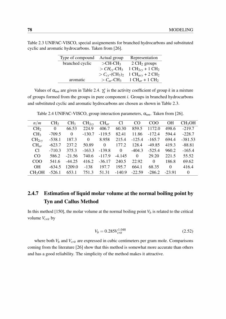
78 MODELING
Table 2.3 UNIFAC-VISCO, special assignements for branched hydrocarbons and substitutedcyclic and aromatic hydrocarbons. Taken from [26].
Type of compound Actual group Representationbranched cyclic >CH-CH3 2 CH2 groups
> CHcy-CH3 1 CH2cy + 1 CH2> Ccy-(CH3)2 1 CHacy + 2 CH2
aromatic > Car-CH3 1 CHar + 1 CH2
Values of αnm are given in Table 2.4. γ∗k is the activity coefficient of group k in a mixtureof groups formed from the groups in pure component i. Groups in branched hydrocarbonsand substituted cyclic and aromatic hydrocarbons are chosen as shown in Table 2.3.
Table 2.4 UNIFAC-VISCO, group interaction parameters, αnm. Taken from [26].
n/m CH2 CH3 CH2cy CHar Cl CO COO OH CH3OHCH2 0 66.53 224.9 406.7 60.30 859.5 1172.0 498.6 -219.7CH3 -709.5 0 -130.7 -119.5 82.41 11.86 -172.4 594.4 -228.7
CH2cy -538.1 187.3 0 8.958 215.4 -125.4 -165.7 694.4 -381.53CHar -623.7 237.2 50.89 0 177.2 128.4 -49.85 419.3 -88.81
Cl -710.3 375.3 -163.3 -139.8 0 -404.3 -525.4 960.2 -165.4CO 586.2 -21.56 740.6 -117.9 -4.145 0 29.20 221.5 55.52
COO 541.6 -44.25 416.2 -36.17 240.5 22.92 0 186.8 69.62OH -634.5 1209.0 -138 197.7 195.7 664.1 68.35 0 416.4
CH3OH -526.1 653.1 751.3 51.31 -140.9 -22.59 -286.2 -23.91 0
2.4.7 Estimation of liquid molar volume at the normal boiling point byTyn and Callus Method
In this method [150], the molar volume at the normal boiling point Vb is related to the criticalvolume Vcrit by
Vb = 0.285V 1.048crit (2.52)
where both Vb and Vcrit are expressed in cubic centimeters per gram mole. Comparisonscoming from the literature [26] show that this method is somewhat more accurate than othersand has a good reliability. The simplicity of the method makes it attractive.

2.4 Computer-aided molecular design (CAMD) techniques 79
2.4.8 Estimation of critical volume by Joback Method
One of the first successful group contribution methods to estimate critical properties wasdeveloped by Lydersen (1955) [151]. Since that time, more experimental values have beenreported and efficient statistical techniques have been developed that allow determination ofalternative group contributions and optimized parameters. The Joback method has the lowesterror, around 3% with better results for larger substances (3 or more carbons) [26].
Joback [152, 153] reevaluated Lydersen’s group contribution scheme, added several newfunctional groups, and determined new contribution values. His relation for the calculationof the critical volume is
Vcrit [cm3mol−1] = 17.5+∑k
Nk(vck) (2.53)
where the contribution part is indicated as vck. The group indentities and Joback’s valuesfor contributions to the critical volume are as follows from Table 2.5.
Table 2.5 Group contributions for calculation of critical volume in Joback Method (1984).Taken from [26].
Group vck [cm3mol−1] Group vck [cm3mol−1]CH3 65 O 18CH2 56 O (ring) 13CH 41 C=O 62C 27 C=O (ring) 55
=CH2 56 CH=O 82=CH 46 COOH 89=C 38 COO 82
=C= 36 =O 36≡CH 46 NH2 38≡C 37 NH 35
CH2 (ring) 48 NH (ring) 29CH (ring) 38 N 9C (ring) 27 =N- X
=CH (ring) 41 =N- (ring) 34=C (ring) 32 =NH X
F 27 CN 91Cl 58 NO2 91Br 71 SH 63I 97 S 54
OH 28 S (ring) 38ACOH -25
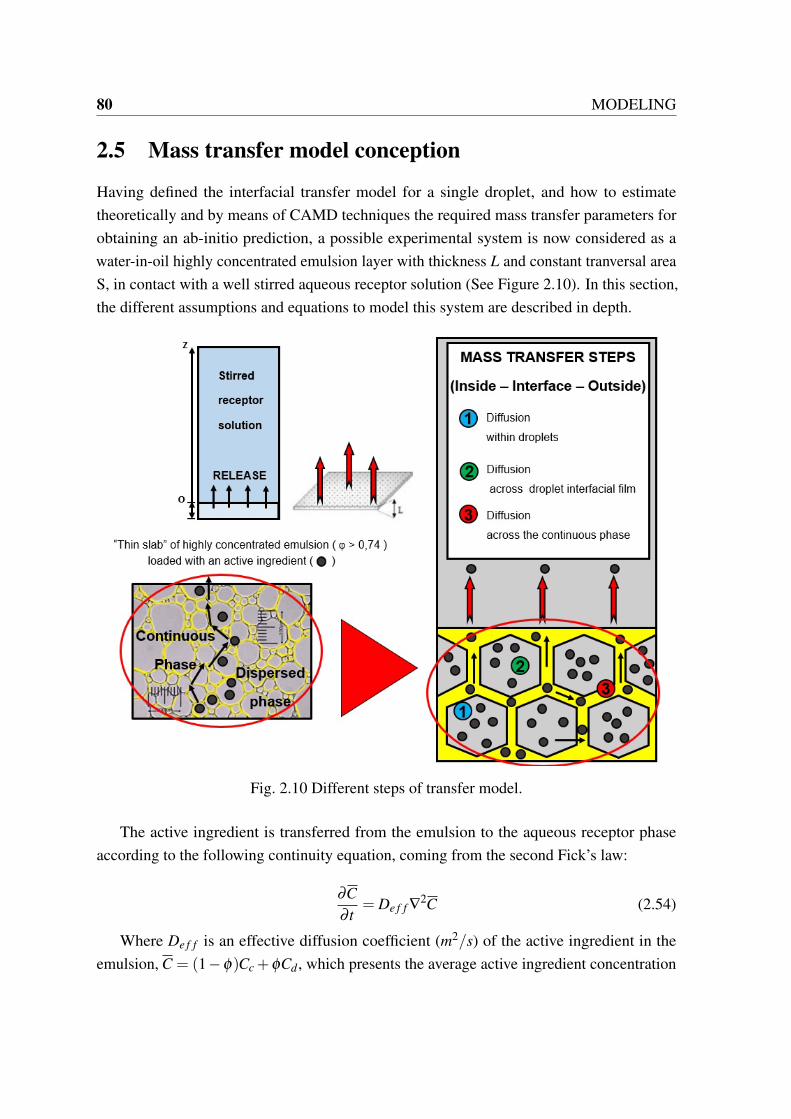
80 MODELING
2.5 Mass transfer model conception
Having defined the interfacial transfer model for a single droplet, and how to estimatetheoretically and by means of CAMD techniques the required mass transfer parameters forobtaining an ab-initio prediction, a possible experimental system is now considered as awater-in-oil highly concentrated emulsion layer with thickness L and constant tranversal areaS, in contact with a well stirred aqueous receptor solution (See Figure 2.10). In this section,the different assumptions and equations to model this system are described in depth.
Fig. 2.10 Different steps of transfer model.
The active ingredient is transferred from the emulsion to the aqueous receptor phaseaccording to the following continuity equation, coming from the second Fick’s law:
∂C∂ t
= De f f ∇2C (2.54)
Where De f f is an effective diffusion coefficient (m2/s) of the active ingredient in theemulsion, C = (1−φ)Cc +φCd , which presents the average active ingredient concentration
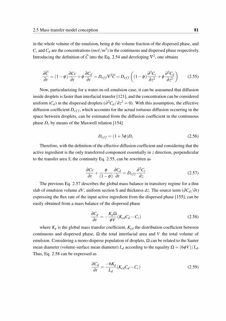
2.5 Mass transfer model conception 81
in the whole volume of the emulsion, being φ the volume fraction of the dispersed phase, andCc and Cd are the concentrations (mol/m3) in the continuous and dispersed phase respectively.Introducing the definition of C into the Eq. 2.54 and developing ∇2, one obtains
∂C∂ t
= (1−φ)∂Cc∂ t
+φ∂Cd
∂ t= De f f ∇
2C = De f f
((1−φ)
∂ 2Cc
∂ z2 +φ∂ 2Cd
∂ z2
)(2.55)
Now, particularizing for a water-in-oil emulsion case, it can be asusumed that diffusioninside droplets is faster than interfacial transfer [121], and the concentration can be considereduniform (Cd) in the dispersed droplets (∂ 2Cd/∂ z2 = 0). With this assumption, the effectivediffusion coefficient De f f , which accounts for the actual tortuous diffusion occurring in thespace between droplets, can be estimated from the diffusion coefficient in the continuousphase Dc by means of the Maxwell relation [154]
De f f = (1+3φ)Dc (2.56)
Therefore, with the definition of the effective diffusion coefficient and considering that theactive ingredient is the only transferred component essentially in z direction, perpendicularto the transfer area S, the continuity Eq. 2.55, can be rewritten as
∂Cc∂ t
+φ
(1−φ)
∂Cd
∂ t= De f f
∂ 2Cc
∂ z(2.57)
The previous Eq. 2.57 describes the global mass balance in transitory regime for a thinslab of emulsion volume dV , uniform section S and thickness dz. The source term (∂Cd/∂ t)expressing the flux rate of the input active ingredient from the dispersed phase [155], can beeasily obtained from a mass balance of the dispersed phase
∂Cd
∂ t=−
KgΩ
φV(KcdCd −Cc) (2.58)
where Kg is the global mass transfer coefficient, Kcd the distribution coefficient betweencontinuous and dispersed phase, Ω the total interfacial area and V the total volume ofemulsion. Considering a mono-disperse population of droplets, Ω can be related to the Sautermean diameter (volume-surface mean diameter) Ld according to the equality Ω = (6φV )/Ld .Thus, Eq. 2.58 can be expressed as
∂Cd
∂ t=
−6Kg
Ld(KcdCd −Cc) (2.59)

82 MODELING
Now, introducing Eq. 2.59 into the global mass balance in transitory regime (Eq. 2.57), itis possible to clear up and arrive to an equation expressing the flux from the continuous phase
∂Cc
∂ t=
6Kgφ
(1−φ)Ld(KcdCd −Cc)+De f f
∂ 2Cc
∂ z2 (2.60)
The resolution of equations 2.60 and 2.59 permits to obtain the concentration profileevolution of active ingredient for each phase and time. The transport model in the emulsionis closed by defining initial and boundary conditions for the dependent variables Cd and Cc.At the beginning, the emulsion phases are supposed to be in their equilibrium concentrations,so that both initial concentrations C0,d and C0,c may be calculated given the initial averageactive ingredient concentration C0, the previous definition of C and the distribution coefficientrelation Kcd giving
C0,d =C0
Kcd(1−φ)+φ; C0,c =
KcdC0
Kcd(1−φ)+φ(2.61)
Concerning the boundary conditions, at z = 0, the concentration of active ingredientis maximum in relation to the coordinate z. In addition, assuming that the volume of thereceptor solution is large enough (infinite volume), the active ingredient gets strongly dilutedwhen it is released, the concentration in the contact surface between the emulsion and thereceptor solution can be considered zero. Therefore
z = 0;∂Cc
∂ z= 0; and z = L ;Cc =Cd = 0; (2.62)
The ensemble of all equations that have been described in this chapter, allows theprediction of the active ingredient release from a highly concentrated emulsion by meansof a mechanistic realistic theory based on Fick’s law of diffusion, taking into account theresistances due to the interfacial layer and continuous phase, and the different equilibriapresent between phases. It is also considered that the diffusion of the active ingredient doesnot affect the structure of the emulsion, as well as all structural parameters are considered tobe constant during the release.
As a remark, it should be noted that the model, although restricted here to a simplethin slab geometry and infinitely diluted solution conditions, it could be, in perspective,easily adapted to different geometries, or conditions, such as a multicomponent mass transfer(where not only an active ingredient was the transferred component) or cases of concentrationdependence for diffusion coefficients.

Chapter 3
SIMULATION
’The mere act of observing something changes the nature of the thing observed’, Heisenberg
3.1 Introduction
Despite of its basis on a clear scientific background, ab-initio simulations performed by modelbuilding, are an art more than a science [156]. However, fortunately, mathematical modelersshare the same procedure [157], consisting in (1) delineating the phenomenon studied, (2)expressing this in mathematical terms, and finally (3) predicting experimental behaviorin different conditions. This means, that if A represents a determined phenomenologicalmanifestation of reality, model building its respective simulation means to find out, insidethe mathematical world, one or more structures able to formally represent and interpret Aallowing the simulation of all possible interactions [158].
In this chapter, the first subsection will consist in an overview of the ab-initio modeldeveloped in this thesis to predict the release of an active ingredient from water in oil highlyconcentrated emulsions, employing and connecting all the theoretical background fromprevious chapter. Different diagrams will try to establish the relations occuring among all thevariables involved. The mathematical programming and all the work on the computer wascarried out using MATLAB®.
After this, an analysis concerning molecular structures of possible candidate chemicalswill be performed in order to create a cartography of materials to work with. An analysis ofsensibility of variables will be performed. Thus, case studies obtained by the operation ofthe ab-initio model by using these materials will reveal the paramount importance for whatconcerns a possible experimental design on the next Chapter 4. Only with a clear knowledgeabout the whole system and its behaviors, it will be possible to decide later experiments,ways to perform them and check the robustness of our ab-initio model.

84 SIMULATION
3.2 Logical Architecture Diagram
This section presents the formal definitions and different steps (as diagrams and relationsbetween variables) of the computer simulation framework. Because the reverse engineeringis based on CAMD techniques, it is necessary to employ some form of representationof the molecular structure information for use in physico-chemical parameter estimation.Consequently, a database is required. This database includes the representation of compoundsas a collection (or vector) of groups. In this work, it has been limited to four the numberof components present in the emulsion: an active ingredient, an oil acting as continuousphase, a dispersed phase (generally, water containing a small proportion of salt for stabilizingpurposes) and a surfactant. However, it is expected that it could be expanded to a highernumber of components (including co-surfactants, viscosity modifiers, etc.) or even to thedomain of oil in water emulsions.
First, a serie of identification numbers (’V knumbers’) that enumerate the components ofa candidate list (cartography database) are proposed. This input, will compile the number ofoccurrences of each atom type conforming the molecule selected (’vk’ integers appearingin previous Eq. 2.22) to be used later for the prediction of activity coefficients by UNIFACand mixture viscosity calculations. Following this, the cartography database has a secondobjective of providing respective molar volumes, molecular weights, pure compound densi-ties/viscosities and the other required geometrical parameters for the calculations (A1*, A2*and A2). It should be mentioned, that in this work, pure compound properties were takenfrom the free chemical structure database [20] of The Royal Society of Chemistry .
Once components and respective physico-chemical properties have been loaded fromthe cartography database, specifications concerning the emulsion formulation are requiredfor a next step. These are the concentration of active ingredient (AI) in the emulsion (massamount per mass of dispersed phase), the dispersed phase mass fraction (φm), the mass ratiobetween oil and surfactant (roil/sur f = moil/msur f .), the total mass prepared of emulsion, theexperimental amount of emulsion utilized for the release, the volume of the receptor solutionand the droplet diameter of dispersed phase. By using all these especifications, and relationsappearing in Fig.3.1 concerning dispersed and continuous phases, the quantities present in athin slab of emulsion are recalculated. Following this, the flash algorithm can be applied inorder to obtain the equilibrium molar fractions and the distribution coefficient of the activeingredient between continuous and dispersed phases. After the convergence, by using therespective molar volumes and equilibrium compositions, phase volumes and the volumetricfraction of dispersed phase are calculated.

3.2 Logical Architecture Diagram 85
Fig. 3.1 Inital steps for selection of components from the cartography database and set-up ofvariables later necessary to simulate the release.

86 SIMULATION
For sake of clarity, in Fig.3.2, the different steps of the flash equilibrium algorithm havebeen outlined, and typical snapshots given by the programming code when applied have beenshown. A more detailed description is given in the following page.
Fig. 3.2 Schematic diagram of stages of the equilibrium flash algorithm and typical responseobtained when it is applied.
DESCRIPTION OF EQUILIBRIUM FLASH ALGORITHM + KEY COMPONENTS TEST
Example of required INFO for calculations:
l st EQUILIBRIUM
FLASH (UNIFAC)
tORDER OF COMPONENTS : ~de1~c ac~d / dodecane 1 wacer 1 span80 q_d•(0 . 02 1 0 1 . ~ 16 OJ ; \INITIAL DISPERSED PHASE
\mass amounc [O] ~n c=O on d1spersed phase q_ c •(O 0 . 076 0 0 . 071] ; \INITIAL CONTINUOUS PHASE
tmass amounc [g] 1n c• O on conc1nuous phase mw- (152 . 15 170 . 33 18 . 015 i28 . 603] ; \MOLECULAR WEIGHTS OF COMPONE!ITS (q/ mol]
m~ ( 115 . 1 227 . 1 0 6 18 ~01 . 1] ;
\MOLAR VOLUMES OF COMPONENTS [cm3/ mol)
Key components test:
Example of typical OUTPUT Kc 1. 579723202795391
p h i 0 . 892. 959011 . 8579
g_comp_eq_c )0.0034 0.0764 9.5521 e·04 0.0711) g_comp_eq_d [0.0177 2.9445. -06 1.4155 3.0754· ·09)
v_total 1.2868 vm_d_eq 1.1484
Responsible components of separation in two phases Ratio of distribution constants (ij)
(ij) combinat ions ::omD_ k e y •
x d -- )~o-. o-o-.7-------------------, o.oon o. 9800 o.oln)
0 . 0067 0 . 0067
0 . 9800 0 . 9800
o. 0067 0 . 0)61 0 . 0067 0 . 0)67 • ~ : :::~
o. 9800
x c -
~)0 .7.00~67~~~~~--~=
o.oon o. 0067 O. M67 0 . 0067 0 . 0067 0 . 0)67
O. OOfi1 o. 0067 O. M67
o.oooo)
(i) (j)
0 . 0067 0 . 0067 0 . 0067 0 . 0067
0 . 0067
0 . 0067
0 . 0067
0 . 0067
0 . 0067 0 . 0067
o. 9800
0 . 0067
0 . 0067 0 . 9800 o. 9800 0 . 0067
0 . 0067 0 . 9800
o. 9800 0.0067
0 . 0067 0 . 0067 Key components:
l . Oe + 0 3 ~
2 . 934222644765270
0 . 000030898971177
0 . 0000000105305•8
0 . 017900317153731
0 . 000006100531323
0 . 51 9317 5 7 8 2 80 6 13
(a ij) calculations
water (i=3) dispersed phase & span80 (j=4) continuous phase
EQUILIBRIUM EVALUATION STAGE
Initial iteration (L2/F) = 0.5 ; f(key components) ; • x_c= 0.0067 0.0067 0.0067 0.9800
x_d= 0.0067 0.0067 0.9800 0.0067
Distribution constants (i)
xL' i ' K· - 1 _ 1
' - x~• - .. ~2 ' Y;
Mass balance
Z; = (1-~) f' + ~J-2 F 1 F 1
Radchford Rice equation
Generation of mathematical model of specified system
Convergence of curve solutions
NUMERICAL SOLUTION
f (ln/ F)- ~ xiJ,-~xL'- ~ z;(K; - l ) . - - 6 i 6 i - ;~ -,-1-+--:-L-'-z/-:-F=( K-:--:1-'-__ ----,1--,--)
Newton-Raphson method Criteria for convergence
( i.) nex1 ilermion = ( i.) -;,~~j~)) IIC
error = [ lx~' If' -x~~~~ tolerance i= l
2300 ······; ······: ······:- ······: ·····: ······: ······: ·····: 2000 ..• ···f ·······f·······~·······f······-~·-·····!·······t·······!·······i
... ~ ~ ~ 1500 .. .. . . • . . .. ..•. --· . . . ...... . ... ... ... . .
w
1000 .
soo .......
•• "' 08 <: 0 0.1 .. i 0.6
... 0.5
"' 0 04
::!: 03
02
·· · ~ · · · · · · ·r · · · · · -~ · · · · · ··l· · · · ·· ·! · · · · · · ·: · · · · · · -~ · · · · · ·· ~
1 j
Evolution of molar fractions solutions
Iterations number

3.2 Logical Architecture Diagram 87
As one can see, the first step consisted of taking couple of components and constitutehypothetical phases, where alternately each one of the components was majority. Thisimplied to take a mole fraction of 0.98 in the dispersed phase (mole fractions compositionsrepresented by x_d) of a possible key component (i), and the rest of composition to bedistributed between the other components, taking care the total sum to be the unity. Similarly,in the continuous phase (mole fractions compositions represented by x_c), it is taken 0.98 forthe composition a component (j), which takes the rol of key component for this phase. Byusing these compositions, the equilibrium relations Ki can be calculated for components iand j, and with them, their respective distribution relations αi j. On completion of this, it isnecessary to ensure that the result will be always greater than unity (if this would not happen,it should be enough to change the order of the couple ij by ji). The procedure is performeduntil all possible combinations of couples in the quaternary mixture are concluded, and fromthis point on, the obtained values are considered as the distribution relations for every couple.
In the second step, the distribution relation values should be compared. As one can seein the graph, the couple of the first line (equivalent to components i = 3, water and j = 4,SPAN 80 in the example), showed the highest value for the ratio of distribution constantα34, therefore, this couple is the candidate couple of key components of the system. Oncedetermined the key components, the initial estimations for compositions of the two phasesare taken; defining each phase rich in its respective key component, with mole fraction of0.98. To the other components, the compositions are assigned until adding up the unity. Aninitial value of 0.5 was employed for the relation of phases L2/F .
Once the equilibrium flash is applied, the presence of surfactant on the interface should betaken into account. For this purpose, the relations appearing in Fig.3.3 are used. Dependingmainly on the mean droplet size of the emulsion and the surface polar head of the surfactantemployed, the surfactant amount on the interface can be easily calculated. This quantityis substracted then from the continuous phase composition in equilibrium that resultedpreviously from the flash. Following this, a second flash equilibrium is applied, but in regardsto the hypothetical equilibrium between the surfactant layer and the dispersed phase. Thisshould be performed in order to work out the hypothetical distribution coefficient of theactive ingredient between an homogeneous layer of surfactant and the dispersed phase, whichis required later for the calculation of the permeability. Calculating the critical volume by theJoback method, one can use it to estimate the volume of the active ingredient at its normalboiling point by means of the Tyn and Callus relation. After this, the diffusivity in puresurfactant, given by the Wilke Chang equation can be determined. It should be noted here,that the viscosity appearing in the denominator, refers to the viscosity of pure surfactant.

88 SIMULATION
Fig. 3.3 Final steps for setting up all required variables for release simulations. Calculationof the global mass transfer resistance.
Next, the global mass transfer resistance is about to be determined. On the one hand, theinterfacial mass transfer is calculated. For this purpose, the diffusivity of the active ingredientis estimated again with the Wilke Chang equation, but in this case, referring to a diffusivity

3.2 Logical Architecture Diagram 89
through the continuous phase. It is remarked here that the viscosity required on the equationis predicted by the UNIFAC-VISCO method. The mean molecular weight corresponding tothe continuous phase, is obtained by weighting the substances present in relation to their massamounts. On the other hand, the permeability of the surfactant layer is also calculated usingthe previous permeability of a disordered layer and the factor for decrease of permeabilitydue to the interfacial order. By way of illustration, it has been shown the dominance of thenormalized surface density within the exponent of the factor for decrease of permeability.
Fig. 3.4 Sixth step and last one of the ab-initio model. The release profile is simulated.
At this point, all parameters required for the simulation of the release profile would havebeen estimated or calculated. Consequently, the model equations can be solved by meansof the function PDEPE on MATLAB®. The ab-initio model predicts the instantaneousflow of active ingredient exiting both phases (continuous and dispersed) and its cumulativepercentage profile (calculated considering a given volume of receptor solution) as functionof time. An example of this prediction can be visualized in Fig.3.4. All parameters involvedduring each simulation are registered and this allows possible comparisons between thedifferent cases. It is also worthy to point out that the time for the resolution of a case study isrelatively fast (less than one second). Therefore, it is expected a low computational cost forthe simulation of a big number of cases .
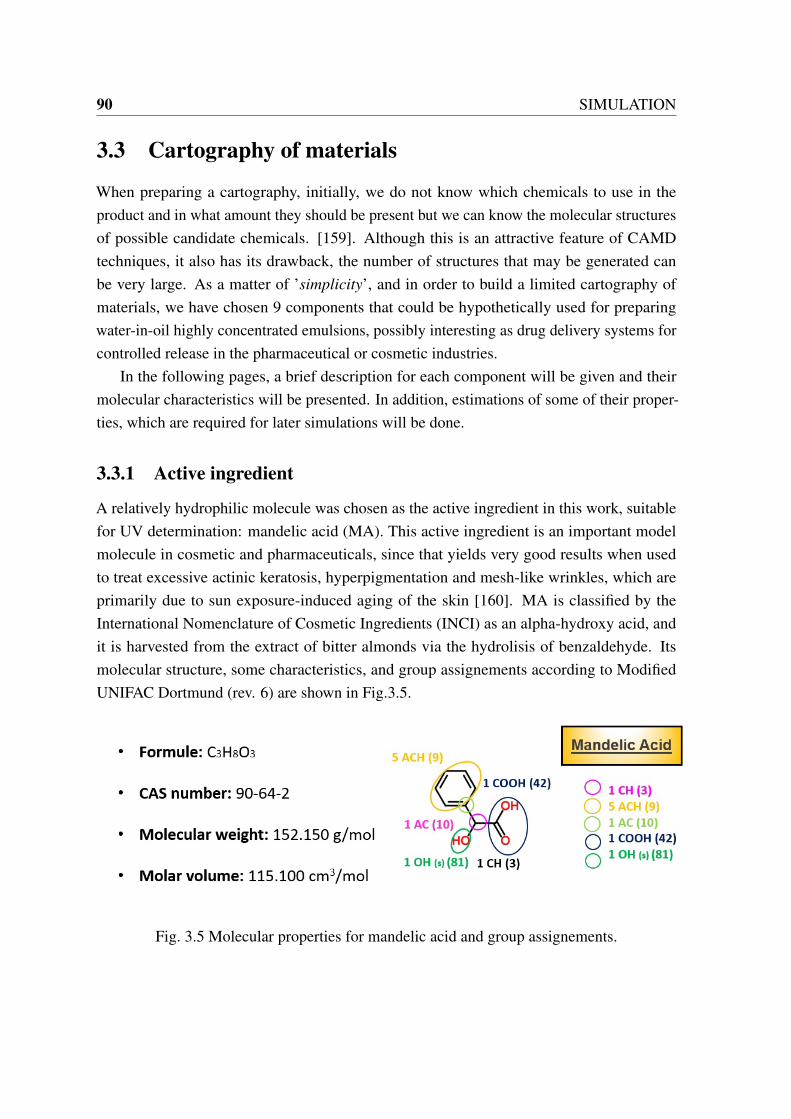
90 SIMULATION
3.3 Cartography of materials
When preparing a cartography, initially, we do not know which chemicals to use in theproduct and in what amount they should be present but we can know the molecular structuresof possible candidate chemicals. [159]. Although this is an attractive feature of CAMDtechniques, it also has its drawback, the number of structures that may be generated canbe very large. As a matter of ’simplicity’, and in order to build a limited cartography ofmaterials, we have chosen 9 components that could be hypothetically used for preparingwater-in-oil highly concentrated emulsions, possibly interesting as drug delivery systems forcontrolled release in the pharmaceutical or cosmetic industries.
In the following pages, a brief description for each component will be given and theirmolecular characteristics will be presented. In addition, estimations of some of their proper-ties, which are required for later simulations will be done.
3.3.1 Active ingredient
A relatively hydrophilic molecule was chosen as the active ingredient in this work, suitablefor UV determination: mandelic acid (MA). This active ingredient is an important modelmolecule in cosmetic and pharmaceuticals, since that yields very good results when usedto treat excessive actinic keratosis, hyperpigmentation and mesh-like wrinkles, which areprimarily due to sun exposure-induced aging of the skin [160]. MA is classified by theInternational Nomenclature of Cosmetic Ingredients (INCI) as an alpha-hydroxy acid, andit is harvested from the extract of bitter almonds via the hydrolisis of benzaldehyde. Itsmolecular structure, some characteristics, and group assignements according to ModifiedUNIFAC Dortmund (rev. 6) are shown in Fig.3.5.
Fig. 3.5 Molecular properties for mandelic acid and group assignements.

3.3 Cartography of materials 91
This molecule is a weak acid (pKa=3.75 [161]), which dissociates in aqueous solutiongiving mandelate ions. The degree of ionization depends obviously on the pH of the medium[162]. At basic pH the formation of mandelate is favored while at acidic pH values, thenonionized species predominate (Fig. 3.6).
Fig. 3.6 MA microspecies distribution as function of pH. Obtained from [20].
A higher pH increases the aqueous solubility of MA, from 181 mg/mL at acidic pHs[163] to 927.81 mg/mL at pH 6.5 [20]. This is easy to understand, thinking on the typicalexpression used by chemists to remember how solvents work; ’Like dissolves like’, thatmeans, that polar dissolves polar; water is polar and mandelate as ionized specie possesses ahigher polarity, therefore, at higher pH will dissolve better in water.
Typical concentrations of MA employed in pharmaceutical applications, range until amax. 10% aqueous solutions [160]. For instance, the pH of a diluted aqueous solution of 1.5g MA / 100 g H2O (1.5 %) shows a pH of 2.7. At this pH, the corresponding distributions ofmicrospecies are shown in Fig. 3.7.

92 SIMULATION
Fig. 3.7 Microspecies of MA at pH 2.7 (1.5 % aqueous solution). Obtained from [20].
The area in a compressed state (A∗1) of MA should be estimated for permeability calcula-
tions in the ab-initio model. Taking as a reference this diluted concentration of 1.5 %, it ispossible to consider that the molecule is mostly presented as nonionized form. Therefore,this area (A∗
1) was estimated by using the VABC method described in previous Section 2.4.5.Table 3.1 shows the group parameters for the vdW volume calculation of the whole molecule.Assuming a spherical shape for the whole molecule, the radius (139.51 Å3) can be easilycalculated (3.217 Å). Then, considering the cross-sectional area of this sphere, one obtains32.521 Å2 as the area in a compressed state (A∗
1).
Table 3.1 Calculation of area in compressed state for MA molecule by VABC method.
Type Number Contribution / unit [Å3] Total contribution [Å3]H 8 7.24 57.92C 8 20.58 164.64O 3 14.71 44.13
bonds (NB) 19 -5.92 -112.48aromatic rings (RA) 1 -14.7 -14.7
nonaromatic rings (RNR) 0 -3.8 0vdW volume 139.51 [Å3/molec]sphere radius 3.217 [Å]
cross-sectional area (A∗1) 3.217 [Å2/molec]

3.3 Cartography of materials 93
In addition, the critical volume of the molecule was also estimated by using the Jobackmethod (Section 2.4.8) for the diffusivity calculations. The following Table 3.2 shows theparameters for this calculation. Using the critical volume obtained (Vcrit = 427.5 cm3/mol),the molar volume (Vb) at the normal boiling point (Tb) solved by the Tyn and Callus relation(Eq. 2.52), gives a molar volume of 162.954 cm3/mol.
Table 3.2 Estimation of critical volume for mandelic acid molecule by Joback method.
Type Number vck [cm3/mol] N(vck)CH2 1 56 56
=CH (ring) 5 41 205OH 1 28 28
=C (ring) 1 32 32COOH 1 89 89
Critical volume (Vcrit) 427.5 [cm3/mol]Normal volume at Tb (Vb) 162.954 [cm3/mol]
3.3.2 Dispersed phase
Due to the aforementioned particularization for a water-in-oil emulsion system when themass transfer model conception was done, the dispersed phase is automatically chosen: water.Fig. 3.8 shows the characteristics, molecular structure and group assignement for water.Nevertheless, it should be mentioned that generally a small amount of electrolytes dissolvedin the aqueous phase (for example NaCl) dramatically increases emulsion stability [164].Stability of the gel-emulsion is important, as the rupture of the gel-emulsion structure wouldgive rise to a massive release of the active ingredient contained in the dispersed drops [162].
Fig. 3.8 Molecular properties for water and group assignement.

94 SIMULATION
3.3.3 Continuous phase
A large number of oils are available, which can be used as components of emulsion systems,but their toxicity, irritation potential, and unclear mechanism of action sometimes limit theiruse. One must choose materials that are biocompatible, nontoxic, and clinically acceptable[165]. In this cartography, a group of four different oils, generally regarded as safe, havebeen included; two saturated n-alkanes (dodecane and hexadecane) and two fatty acid esters(isopropyl myristate and isopropyl palmitate). In Fig. 3.9, the molecular properties for thetwo n-alkanes and group assignements according to Modified UNIFAC Dortmund (rev. 6)are shown.
Fig. 3.9 Molecular properties for n-alkanes: dodecane/hexadecane and group assignements.
The production of dodecane and hexadecane as pure chemicals and high-purity processstreams is quite small relative to the petroleum substances (i.e., kerosene, jet fuel, homeheating oil, hydrocarbon solvents) that contain these these n-alkanes as constituents. Almostall (99%) of the purified n-alkane production is not as single chemicals but as process streamsthat contain a range of n-alkanes, typically C10-C13, C12-C14, C12-C16 and C14-C16 [166].These n-alkane process streams are consumed as closed-system chemical intermediates in themanufacture of linear alkylbenzenes, which are chemical building blocks for the manufactureof detergents. In fact, a very small volume is produced in pure form. There are no known

3.3 Cartography of materials 95
consumer product applications for pure dodecane or hexadecane. However, they can bepresent in some hydrocarbon-containing products such as baby oils, sunscreens, hair oils,body and massage oils, makeup removers, some automotive chemicals, cleaning solvents,water repellents used for decks, shoes and sports equipment, and general-use household oilproducts [166].
Fig. 3.10 Molecular properties for fatty acid esters: isopropyl myristate/palmitate, and groupassignements.
Regards the fatty acids esters: isopropyl myristate/palmitate, they are esters of isopropylalcohol and myristic/palmitic acid, respectively. In Fig. 3.10, their molecular propertiesand group assignements according to Modified UNIFAC Dortmund (rev. 6) are shown.They are commercially produced by distillation, which is preceded by the esterification ofmyristic/palmitic acid and isopropanol, in the presence of an acid catalyst. The product isstripped to remove excess isopropanol, alkali refined to neutralize the catalyst, and the productis then distilled to obtain isopropyl myristate/palmitate [167]. They are very important assolubilizing, spreading, and penetrating agents in anhydrous skin lubricating lotions. Theseesters leave the skin soft and smooth without an oily surface film. Therefore, they aretypically used in bath oils, perfumes, creams, lotions, lipsticks, hair preparations, shavinglotions, aerosol toiletries, and pharmaceutical ointments.

96 SIMULATION
3.3.4 Surfactants
Similarly to the oils for the continuous phase, one should use emulsifiers in an appropriateconcentration range that will result in mild and nonaggressive emulsions. The surfactantchosen must be able to lower the interfacial tension to a very small value, which facilitatesdispersion process during the preparation of the highly concentrated emulsion, providing aflexible film that can readily deform around the droplets. Also it must be of the appropriatelipophilic character to provide the correct curvature at the interfacial region [165].
As it is well known in the art, the terms ’hydrophilic’ and ’lipophilic’ are relativeterms. To function as a surfactant, a compound must necessarily include polar hydrophilicmoieties as well as non-polar hydrophobic (lipophilic) moieties; i.e., a surfactant compoundmust be amphiphilic. An empirical parameter commonly used to characterize the relativehydrophilicity and lipophilicity of non-ionic amphiphilic compunds is the hydrophilic-lipophilic balance (the ’HLB’ value). Surfactants with lower HLB values are more lipophilic,and have greater solubility in oils, whereas surfactants with higher HLB values are morehydrophilic, and have greater solubility in aqueous solutions [168]. The HLB of a surfactantcan be an useful guide for surfactant selection. It is generally accepted that low HLBsurfactants are favored for the formulation of w/o emulsions, whereas surfactants with highHLB (>12) are preferred for the formation of o/w emulsions [165].
In this work, three different types of surfactants (Fig. 3.11) have been chosen, withan appropriate HLB (at least, expected initially) in relation to the oils of the previoussection: a sorbitan fatty acid ester (sorbitan monooleate, SPAN 80 ®), a polyglycerizedfatty acid (polyglycerol polyricinoleate, PGPR ®) and a polyethylene glycol alkyl ether(polyoxyethylene glycol-2-oleyl ether, BRIJ 93 ®).
1. Sorbitan monooleate is a sorbitan ester of Croda, marketed under the Span productname (SPAN 80 ®). It is produced by the dehydration of sorbitol and esterificationwith oleic acid (mono) in a controlled chemical process. As nonionic surfactant, itoffers increased stability, formulating flexibility and wider compatibility. It is stable inmild acids, alkalis and electrolytes and do not react with ionic ingredients or actives.This surfactant is a key emulsifying agent for a number of applications in householdconsumer products, excellent for water in oil emulsification of hydrocarbons and usefulas solubiliser, wetting agent and dispersant.
2. Polyglycerol polyricinoleate (PGPR), is a food grade emulsifier consisting of poly-glycerol as the hydrophilic group (mainly found a 75% as di- tri- or tetraglycerol) andinteresterified ricinoleic fatty acids as the hydrophobic group. In Fig. 3.11, the typicalstructure of the fraction consisting of tri-glycerol tri-ricinoleate is shown. PGPR is

3.3 Cartography of materials 97
Fig. 3.11 Group assignements and molecular properties for surfactants included in thecartography.
• Formule: C24H4406
• CAS number: 1338-43-8 • Molecular weight: 428.603 g/mol • Molar volume: 401.100 cm3/ mol • HLB: 4.3 • Density: 1.1 g/ cm3
• Normal boiling point: 579.3 ·c • Index of refraction: 1.4765 • Viscosity (2s•q: 818.733 mPa·s
• Formule: C63Hn60t3
• CAS number: 68936-89-• Molecular weight: 1081.587 g/ mol • Molar volume: 1019.407 cm3/mol • HLB: 3-6 • Density: 1.061 g/cm3
• Normal boiling point: 416.4 ·c • Index of refraction: 1.4770 • Viscosity (25°C): 4209.8 mPa·s
• Formule: C63Hn6013
• CAS number: 9004-98-2 • Molecular weight: 356.580 g/ mol • Molar volume: 248.684 cm3/ mol • HLB: 4 • Density: 0.912 g/cm3
• Normal boiling point: 100 ·c • Index of refraction: 1.4595 • Viscosity (2s•q: 27.767 mPa·s
Sorbitan monooleate (SPAN 80)
0 1 CH3(1)
0 14CHz(2)
0 1 CHzCOO (22)
0 1 CHz0(25)
0 1 CH (3) 0 3 c-CH (79)
0 1 CH=CH 6) 0 3 OH !•J (81)
Polyglvcerol polyricinoleate (PGPR)
0 3 CH3 (1) 0 3 CH=CH (6) 0 2 CHzO (25)
0 40 CHz (2) 0 1 OH !Pl (14) 0 4 OH !•l (81)
0 6 CH (3) 0 3 CHzCOO (22)
Polyoxyethylene glycol-2-oleyl ether (BRIJ 93)
0 1 CH3 (1)
0 14CHz (2)
0 1CH=CH(6
0 1 OH !Pl (14)
0 2 CHz0(25)

98 SIMULATION
widely known as an excellent water in oil emulsifier. It is used to manufacture stablepan release agents for the bakery industry and to stabilize low fat margarine systemswith high water content. However, the main application of PGPR is in the chocolateindustry, because it has the ability for improving the flow properties by lowering thefriction between the particles suspended in the liquid fat phase.
3. Polyoxyethylene glycol-2-oleyl ether (also known as Oleth-2 or by its commercialname, BRIJ 93 ®, registered trademark of Croda) is an alkyl PEG ether, reactionproduct of an alkyl alcohol (oleyl alcohol) and two equivalents of ethylene oxide [169].It is an exceptional nonionic water in oil emulsifier and recommended for a wide rangeof topical applications within cosmetic and personal care products, such as body andhand creams, hair conditioners, hair dyes, lotions and deodorants. Its nonionic natureallows flexibility in formulation and provides compatibility over a wide pH range. Itacts as a wetter, co-emulsifier and solubiliser of oils.
Since it is required for permeability calculations, the area per molecule in a compressedmonolayer (A∗
2), as well as the actual area per molecule (A2) for each one of the surfactantswill be estimated by using the VABC method. It should be noticed that A2 has been workedout in a similar manner as previously done for the active ingredient mandelic acid (consideringthe whole molecule), but for the estimation of A∗
2, only the polar part (polar surface area)of the molecules have been taken into account. The next Fig. 3.12 emphasizes the partsconsidered in the calculation of polar areas (A∗
2) of surfactants. The following Tables from3.3 to 3.5 reflect the work out of these polar areas.
Fig. 3.12 Considered polar parts for each surfactant of the cartography in this work.

3.3 Cartography of materials 99
Table 3.3 Calculation of polar area (A∗2) for SPAN80 by VABC method.
Type Number Contribution / unit [Å3] Total contribution [Å3]H 9 7.24 65.16C 5 20.58 102.9O 4 14.71 58.84
bonds (NB) 18 -5.92 -106.56aromatic rings (RA) 0 -14.7 0
nonaromatic rings (RNR) 1 -3.8 -3.8vdW volume 116.54 [Å3/molec]sphere radius 3.030 [Å]
polar area (A∗2) 28.845 [Å2/molec]
Table 3.4 Calculation of polar area (A∗2) for PGPR by VABC method.
Type Number Contribution / unit [Å3] Total contribution [Å3]H 19 7.24 137.56C 10 20.58 205.8O 8 14.71 117.68
bonds (NB) 36 -5.92 -213.12aromatic rings (RA) 0 -14.7 0
nonaromatic rings (RNR) 0 -3.8 0vdW volume [Å3/molec] 247.92
sphere radius 3.897 [Å]polar area (A∗
2) 47.712 [Å2/molec]
Table 3.5 Calculation of polar area (A∗2) for BRIJ93 by VABC method.
Type Number Contribution / unit [Å3] Total contribution [Å3]H 9 7.24 65.16C 4 20.58 82.32O 3 14.71 44.13
bonds (NB) 15 -5.92 -88.8aromatic rings (RA) 0 -14.7 0
nonaromatic rings (RNR) 0 -3.8 0vdW volume [Å3/molec] 102.81
sphere radius 2.906 [Å]polar area (A∗
2) 26.532 [Å2/molec]
Now, in Tables from 3.6 to 3.8, the calculation was performed based on the wholemolecule of each surfactant in order to obtain the actual area per molecule (A2).

100 SIMULATION
Table 3.6 Calculation of actual area per molecule (A2) for SPAN 80 by VABC method.
Type Number Contribution / unit [Å3] Total contribution [Å3]H 44 7.24 318.56C 24 20.58 493.92O 6 14.71 88.26
bonds (NB) 74 -5.92 -438.08aromatic rings (RA) 0 -14.7 0
nonaromatic rings (RNR) 1 -3.8 -3.8vdW volume 458.86 [Å3/molec]sphere radius 4.784 [Å]
cross-sectional area (A2) 71.924 [Å2/molec]
Table 3.7 Calculation of actual area per molecule (A2) for PGPR by VABC method.
Type Number Contribution / unit [Å3] Total contribution [Å3]H 115 7.24 832.6C 63 20.58 1296.54O 13 14.71 191.23
bonds (NB) 190 -5.92 -1124.8aromatic rings (RA) 0 -14.7 0
nonaromatic rings (RNR) 0 -3.8 0vdW volume 1195.57 [Å3/molec]sphere radius 6.584 [Å]
cross-sectional area (A2) 136.190 [Å2/molec]
Table 3.8 Calculation of actual area per molecule (A2) for BRIJ 93 by VABC method.
Type Number Contribution / unit [Å3] Total contribution [Å3]H 44 7.24 318.56C 22 20.58 452.76O 3 14.71 44.13
bonds (NB) 68 -5.92 -402.56aromatic rings (RA) 0 -14.7 0
nonaromatic rings (RNR) 0 -3.8 0vdW volume 412.89 [Å3/molec]sphere radius 4.619 [Å]
cross-sectional area (A2) 67.036 [Å2/molec]
Up to here, all required parameters necessary for simulations have been compiled orcalculated. In Appendix B, all the data have been classified together as a cartographysummary. This allows a comparison of the components and their respective parameters.

3.4 Objetives of a sensitivity analysis 101
3.4 Objetives of a sensitivity analysis
Sensitivity analysis is the study of how the uncertainty in the output of a mathematical modelor system can be apportioned to different sources of uncertainty in its inputs [170]. Theprocess of recalculating outcomes under alternative assumptions to determine the impact of avariable under sensitivity analysis can be useful for a range of purposes [171], including:
1. Testing the robustness of the results of a model or system in the presence of uncertainty.
2. Increased understanding of the relationships between input and output variables in asystem or model.
3. Uncertainty reduction, through the identification of model inputs that cause significantuncertainty in the output and should therefore be the focus of attention in order toincrease robustness.
4. Searching for errors in the model by encountering unexpected relationships betweeninputs and outputs.
5. Model simplification – fixing model inputs that have no effect on the output, oridentifying and removing redundant parts of the model structure.
6. Finding regions in the space of input factors for which the model output is eithermaximum or minimum or meets some optimum criterion.
7. In case of calibrating models with large number of parameters, a primary sensitivitytest can ease the calibration stage by focusing on the sensitive parameters. Not knowingthe sensitivity of parameters can result in time being uselessly spent on non-sensitiveones [172].
8. To seek to identify important connections between observations, model inputs, andpredictions or forecasts, leading to the development of better models [173, 174].
Good modeling practice needs that the modeler provides an evaluation of the confidencein the model. This requires an evaluation of how much each input is contributing to theoutput uncertainty [170]. Sensitivity analysis addresses this issue, performing the role ofordering by importance the strength and relevance of the inputs in determining the variationin the output. In models involving many input variables, as the current being developedin this work, sensitivity analysis is an essential ingredient of model building and qualityassurance. There are a large number of approaches to performing a sensitivity analysis [170].In general, however, most procedures adhere to the following outline:

102 SIMULATION
1. Identify the model output to be analyzed.
2. Quantify the uncertainty in each input.
3. Run the model a number of times using some design of experiments.
4. Using the resulting model outputs, calculate the sensitivity measures of interest.
In some cases this procedure will be repeated, for example in high-dimensional problemswhere the user has to screen out unimportant variables before performing a full sensitivityanalysis.
3.4.1 Preparation of Virtual Design of Experiments (VDOE)
The capabilities of a design of experiments (DOE), provide a method for simultaneouslyinvestigating the effects of multiple variables on an output variable (response). Theseexperiments consist of a series of runs, or tests, in which purposeful changes are made toinput variables or factors, and data are collected at each run. In this work, by using theab-initio model , the experiments can be conducted virtually (DOE becomes VDOE), and asa consequence, the model itself and the cartography of materials delimited in this chaptercan be qualitatively and quantitatively evaluated.
It is important to recognize that virtual experiments are not the same as live experiments,they are only simulations. However, the cost of doing them is minimal compared with liveexperiments and the process of identifying input and output variables, decided at whichlevel to test, sistematically reviews the interactions between them, aiming to provide claritysurrounding their roles. In addition, virtual experiments allow a great deal into the context of’what if?’ analysis, which may stimulate creative thinking [175], and the research questionof which one is the best configuration of inputs to get the optimal or desired output can alsobe examined.
For characterization of the response coming from the ab-initio model, the solver ’lsqcurve-fit’ of MATLAB® was employed. This tool solves nonlinear curve-fitting (data-fitting)problems in least-squares sense [176], by using the Levenberg-Marquardt method [177].Given an input data xdata, the observed output ydata, where xdata and ydata are vectors, andF(x,xdata) is a vector-valued function of the same size as ydata, mathematically, lsqcurvefitfinds coefficients x that solve the problem:
minx||F(x,xdata)− ydata||22 = min
x ∑i(F(x,xdatai)− ydatai)
2 (3.1)

3.4 Objetives of a sensitivity analysis 103
Considering F(x,xdatai) as the exact analytical solution of Fick’s law for monolithicdevices and thin slab geometry (Eq. 3.2), x the Fickian diffusion coefficient D, xdatai thetime, and ydatai the Mt/M∞ values coming from a virtual experiment, it is possible to fit asimulated release curve in order to obtain a representative D which characterizes the response.
Mt
M∞
= 1− 8π2
∞
∑n=0
exp[−D(2n+1)2π2t/L2]
(2n+1)2 (3.2)
However, when using the solver lsqcurvefit one should bear in mind that the Levenberg-Marquardt method possesses a strong dependency of initial guess values in order to find theglobal minimum and not a local one of the problem. For this purpose, it was decided toclear up possible solution values of Fickian diffusion coefficients using the Eq. 3.2 at n =0, employing the Mt/M∞ values coming from a simulated response given by the ab-initiomodel. In this way, applying the solver lsqcurvefit with these possible diffusion coefficientsolutions as initial guesses, one can easily obtain the best fitting of the curve by taking thevalue which provides the minimum residual from Eq. 3.1.
Fig. 3.13 Evolution of residuals from fitting and comparison between response and fittingcurve.
By way of illustration, Fig. 3.13 shows an example of the evolution of the residual valuesin a data fitting. As one can see in the left graph, the fitting residuals decrease as long as theglobal minimum is found. The last points of possible diffusion coefficient solutions showingthe lowest residual are those coming from the final time of the ab-initio model response. Inthe right graph, one can see the respective response curve and its fitting. Clearly, it can beseen that the fitting tool works quite good. In addition, the time for a case study fitting takesaround 3 seconds.

104 SIMULATION
Once the model output to be analyzed has been identified (D), the factors to test (inputs)as well as their levels need to be decided. According to the scheme showed previously in Fig.3.1, the possible factors to be considered in the VDOE are:
• Concentration of active ingredient,
• Dispersed-phase mass fraction,
• Oil-surfactant ratio,
• Droplet diameter,
• Total mass of emulsion during preparation
• Mass employed for the release experiment,
• Volume of the receptor solution,
• Temperature during release experiment (it is considered that this temperature would bethe same as the one of the preparation),
• Type of oil employed,
• Type of surfactant employed.
The design of experiments is about identifying which is the combination of the previousfactors that could provide a different release curve. At a glance, some of these factors can beeasily dismissed or fixed because they will not affect to the predictions of the ab-initio modelor would not be practical for comparison or experimental or purposes:
• For example, the total mass of emulsion during preparation is obvious that would notgive a different response whatever the amount prepared. However, this interpretationis not comparable to the mass employed for a release experiment. It is clear that themore amount employed, the more would be the delay on the release curve, but forcomparison purposes, changing this variable is not useful, since that even though thecurves delayed on time, all of them would give the same diffusion coefficients. Forthis reason it was suggested to use a basis of one gram as reference.
• On the other hand, the prediction of the ab-initio model is independent of the volumeof the receptor solution, since it is considered to be maintaned at a zero constantconcentration. Nevertheless, for an upcoming experimental part, it is important to bearin mind that to maintain sink conditions, the concentration of an active ingredient in

3.4 Objetives of a sensitivity analysis 105
the receptor solution should be kept below 10% of its concentration in the deliveryvehicle [178]. For verification purposes, change of this variable can be useful.
• Concerning the temperature, a controlled delivery device is generally considered to bedesigned for a specific working temperature. Therefore, it was suggested to keep itconstant as variable. A reference temperature of 25C was chosen.
After these considerations, the VDOE can be adequately planified taking into account theremaining six factors.
3.4.2 Preliminar analysis of VDOE : 64 case studies
In a two-level full factorial design, each experiment factor has only two levels. The exper-imental runs include all combinations of these factor levels. Although two-level factorialdesigns are unable to explore fully a wide region in the factor space, they provide usefulinformation for relatively few runs per factor and can indicate major trends. Thus, it wasdecided to use a two-level full factorial design as a preliminar analysis to provide directionfor a later full factorial design of more levels. Taking into account the six factors, this isequivalent to 26 = 64 possible factor combinations. The following low and high levels shownin Table 3.9 were considered for a first preliminar analysis. They were chosen as typicalencountered values when preparing highly concentrated emulsions. In the case of type of oilor surfactant, variables of text type, only two representative examples from the cartographywere taken.
Table 3.9 Creation of factorial design with 64 combinations. Factor level values.
Factor Low level High levelAI concentration [g AI / g H2O] 0.015 0.050
Dipersed-phase mass fraction [adim.] 0.75 0.95Oil-surfactant ratio [adim.] 1 10
Droplet diameter [m] 0.000005 (5µm) 0.00002 (20µm)Type of oil Dodecane Isopropyl myristate
Type of surfactant SPAN 80 PGPR
The ensemble of the predicted release curves are shown in Figs. 3.14a. The respectiveFickian diffusion coefficients obtained by fitting are represented in Fig. 3.14b. As one can see,different groups of predicted release curves were obtained, with diffusion coefficients rangingfrom 3.78·10−11 to 5.82·10−10 m2/s. However, it appeared that some factor combinationsalmost did not affect to the diffusion coefficient or gave equivalent results.

106 SIMULATION
(a) Predicted release curves of two-level full factorial design.
(b) Run chart of diffusion coefficients obtained by curve fitting.
Fig. 3.14 Simulation results from preliminar VDOE analysis (64 factor combinations).
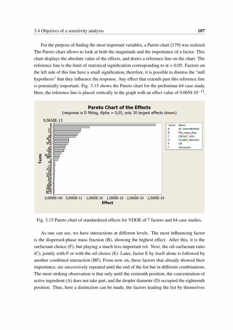
3.4 Objetives of a sensitivity analysis 107
For the purpose of finding the most important variables, a Pareto chart [179] was realized.The Pareto chart allows to look at both the magnitude and the importance of a factor. Thischart displays the absolute value of the effects, and draws a reference line on the chart. Thereference line is the limit of statistical signification corresponding to α = 0.05. Factors onthe left side of this line have a small signification, therefore, it is possible to dismiss the "nullhypothesis" that they influence the response. Any effect that extends past this reference lineis potentially important. Fig. 3.15 shows the Pareto chart for the preliminar 64 case study.Here, the reference line is placed vertically in the graph with an effect value of 9.0658·10−13.
Fig. 3.15 Pareto chart of standardized effects for VDOE of 7 factors and 64 case studies.
As one can see, we have interactions at different levels. The most influencing factoris the dispersed-phase mass fraction (B), showing the highest effect. After this, it is thesurfactant choice (F), but playing a much less important rol. Next, the oil-surfactant ratio(C), jointly with F or with the oil choice (E). Later, factor E by itself alone is followed byanother combined interaction (BF). From now on, these factors that already showed theirimportance, are successively repeated until the end of the list but in different combinations.The most striking observation is that only until the sixteenth position, the concentration ofactive ingredient (A) does not take part, and the droplet diameter (D) occupied the eighteenthposition. Thus, here a distinction can be made, the factors leading the list by themselves

108 SIMULATION
alone or jointly with others (B, C, E and F), can be considered as the most important factorswhich really influence the active ingredient release. In contrast, the last appearing factors (Aand D), can be considered as unimportant variables, since they do not influence significantlythe response of the model. For this reason, they were dismissed for posterior analysis.
3.4.3 Main effects and interaction plots of VDOE : 300 case studies
After the four most important variables have been found, a more complex sensitivity analysiscan be performed. From this point forward, the whole cartography of materials (4 oils and3 surfactants) was considered. In addition, for further analysis, it was allowed more thantwo levels of variation per factor. The following Table 3.10 summarizes the inputs and theirrespective levels employed for a second VODE consisting of 300 simulations. The variableswhich were known that do not influence significantly the response of the ab-initio modelwere kept constant for every case study, such as a concentration of 0.015 g AI / g H2O, or a 5µm droplet diameter. The temperature was also kept at 298 K.
Table 3.10 Creation of factorial design with 300 combinations. Factor level values.
Factor LevelsDipersed-phase mass fraction [adim.] 0.75 / 0.8 / 0.85 / 0.9 / 0.95
Oil-surfactant ratio [adim.] 1 / 2.5 / 5 / 7.5 / 10Type of oil Dodecane / Hexadecane / Myristate / Palmitate
Type of surfactant SPAN 80 / PGPR / BRIJ 93
The simulated release curves, obtained by this VDOE of 300 simulations, are depictedin Fig. 3.16a. Their respective numerical values of diffusion coefficients are shown in Fig.3.16b. As one can see, a wider spectra was obtained in comparison with the previous onefrom the preliminar analysis. Apparently, it seemed that it is possible to completely cover awide region on time by suitable manipulation of the emulsion specifications. The total timefor the full simulation of 300 case studies was around 16 minutes and 20 seconds, which isequal to three seconds per case, relatively a very small amount of computational effort.
The main effects as well as the most important interactions between levels and factorsof the current VDOE are plotted in Fig. 3.17. It is important to keep in mind, that valuesshown in these plots are not absolute values, but the mean of the respective Fickean diffusioncoefficients obtained by fitting of the curves. However, they can give much information aboutthe major tendencies.
As it is shown in the upper graph 3.17a, the dispersed-phase mass fraction is the factorwhich influences the most, and in a linear fashion, the value of the Fickian diffusion coefficientD. The more the value of the dispersed-phase mass fraction, the less the fitting diffusion

3.4 Objetives of a sensitivity analysis 109
(a) Predicted release curves of two-level full factorial design.
(b) Run chart of diffusion coefficients obtained by curve fitting.
Fig. 3.16 Simulation results for VDOE analysis (300 factor combinations).

110 SIMULATION
(a) Main effects plot.
(b) Interaction plot for D fitting.
Fig. 3.17 Simulation results for VDOE analysis of 300 case studies (only the 4 most importantfactors are shown).

3.5 Conclusions of sensitivity analysis 111
coefficient. The oil choice of hexadecane or isopropyl myristate, apparently, shows acomparable influence. This does not happen when changing from dodecane to isopropylpalmitate. Concerning the surfactant, when the surfactant SPAN 80 is employed, the D valuesare generally smaller than those obtained when using other surfactants. On the other hand,the oil-surfactant ratio seems like to influence very slightly the diffusion coefficient value,only small variations were observed at the lowest oil surfactant ratios.
The interactions between individual factors are presented in Fig. 3.17b. In this graph, itis possible to see some important aspects, taking into account that the more parallel the lines,the less significative interactions. Here, one can see that the most pronounced interactionsof the dispersed-mass fraction are those in relation to the choice of oil or surfactant. Thebiggest differences are better observed when a low fraction is used. On the contrary, ifthe dispersed-phase mass fraction employed is relatively high, it appears that there is nosignificant effect on the diffusion coefficient, whatever surfactant, oil, or ratio between themis chosen. Concerning interactions related to the oil-surfactant ratio, it is interesting to notethat only low ratios appear to show a significant effect on the diffusion coefficient D. Incontrast, at high ratios, whatever the surfactant or oil is chosen, the effect on the diffusioncoefficient is equivalent. Concerning the oil choice, generally the predicted release curvesfor emulsions using dodecane as oil offer the higher diffusion coefficients.
3.5 Conclusions of sensitivity analysis
All the modeling developed in previous chapter has been assembled as a complete fullab-initio model. A cartography of materials has been implemented and simulations havebeen performed in order to test the sensitivity of the model.
The sensitivity analysis has given an account of the possible release curves that could beobtained by using the materials composing the cartography and different specifications ofa given highly concentrated emulsion formulation. This information can be used to designtargetted products aimed at a desired controlled release rate, or to compare different productsthat could behave in a similar manner. Besides, the ab-initio model developed in this chaptercould be considered as a very powerful tool that might help enormously for decision makingor intensification-oriented purposes.
However, the possible results to be obtained are limited by the size of the cartography. Itis very likely that the materials of the formulation will restrict the release curves aiming toobtain. In addition, future trials should assess the conclusions obtained.


Chapter 4
EXPERIMENTAL VALIDATIONS
’There are three principal means of acquiring knowledge; observation of nature, reflection,and experimentation. Observation collects facts; reflection combines them; experimentationverifies the result of that combination’, Denis Diderot
4.1 Introduction
The theory developed in this work for mass transfer in highly concentrated emulsions systems,and the predictions from it must be tested with specific experiments designed to confirmor deny their truth. This is fundamental under the reverse engineering approach of thisthesis. As it has been shown in the previous chapter, it is possible to obtain different releasecurves by using specific combinations of dispersed mass fraction, oil, surfactant and theirratios. The success of the reverse engineering of this work, will depend on the accuracy ofthese predictions to be considered as hypothetical design solutions depending on formulationvariables.
Therefore, this chapter aims to address the following research questions:
• are the predictions by UNIFAC models accurate enough to predict the distributioncoefficient of active ingredient between the phases of an emulsion?
• is it possible to predict the viscosity of oil/surfactant mixtures by UNIFAC-VISCOadequately?
• and last and most important, is the ensemble of all the modeling and simulation toolsaccurate enough to trust in the ab-initio model as serviceable tool for product design?

114 EXPERIMENTAL VALIDATIONS
4.2 Predicted and experimental distribution coefficients
As it was seen in the modeling chapter, it is essential to evaluate and understand the partitionof active ingredient in both phases. Since the active ingredient employed in this workabsorbs in the UV region when solubilized in water, UV-visible spectroscopy is presentedas one of the most practical techniques for determining its concentration. The interestedreader may consult the Appendix C, which provides complete details about the experimentalwork performed. Here, only the most important results and conclusions from the tests willbe presented concerning the following subjects: comparison of predictions performed byUNIFAC methods, effect of content of salt on predictions, influence of blank/dilution media,and detection limits of the technique.
4.2.1 Comparison of UNIFAC methods
A preliminar study to determine the effect of the surfactant, water, oil, active ingredient andsalt amounts on the distribution coefficient was carried out. For this purpose, the system: MA+ SPAN 80 + Dodecane + Water was used as a reference. Generally, they were composedby amounts and proportions imitating highly concentrated emulsions. For this reason, fromnow on, the aqueous phase will be named dispersed phase and the organic phase continuousphase. In Fig. 4.1 the predictions for equilibrium concentrations in the dispersed phase, aswell as the distribution coefficients given by the three UNIFAC methods previously reviewedin section 2.4, are shown and compared with the experimental results:
(a) (b)
Fig. 4.1 a) Predicted versus experimental concentrations in dispersed phase. b) Experimentalversus predicted distribution coefficients. Samples characteristics and relative errors betweenpredicted and experimental distribution coefficients are detailed in Table C.1 of AppendixC.0.2.

4.2 Predicted and experimental distribution coefficients 115
As one can see in Fig. 4.1, when using UNIFAC (Fredenslund) model, predictionswere farther from experimental values. Next, in Fig. 4.2 the experimental and predictedconcentrations per sample are shown. Overall, the best precision was obtained when usingModified UNIFAC models, more specifically when using the Addendum Rev/Ext 6 ofContastinescu (2016). The factors which may explain the relatively good correlation betweenthe predicted and experimentally determined concentrations/distribution coefficients whenusing Modified UNIFAC are the following:
• The thermodynamic mixture data stored in the group interaction parameters of UNIFACare mostly coming from vapor-liquid equilibrium data and not from liquid-liquid.Generally, there is an improvement for liquid-liquid equilibrium data sets when passingfrom UNIFAC to Modified UNIFAC. On the other hand, as it was previously seenin section 2.4.2, the combinatorial part of UNIFAC (Fredenslund) is not modifiedempirically to deal with compunds very different in size as it was done for the laterModified UNIFAC versions.
• In addition, the temperature dependent parameters anm, bnm, and cnm from the binaryparameter matrix of Modified UNIFAC, allows a better description of the miscibilitygap. The more updated version, the better the accuracy.
(a) (b)
Fig. 4.2 Predicted versus experimental concentrations in dispersed phase (a); and in continu-ous phase (b). Samples characteristics are detailed in Table C.1 of Appendix C.0.2.
It should be mentioned that the mole amounts of active ingredient in the continuous phasewere worked out by mass balance of the initial weighted mass amounts. For the calculationof concentration in the continuous phase, it was considered a total continuous phase volume(volume of oil + volume of surfactant) same as the one at the moment of sample preparation.
116 EXPERIMENTAL VALIDATIONS
Some important conclusions were drawn from the present study:
• The combination of results provided some support for the conceptual premise that theModified UNIFAC method of Contastinescu (2016) is the most suitable for predictingthe distribution coefficients from the three methods studied because of the betterprecisions obtained. For this reason, it was chosen as the UNIFAC method employedfor the following experiments and later simulations.
• Generally, it was found that in samples with a less amount of surfactant, the precisionobtained between experimental and predicted values was much better. This result mightbe related to the interference observed during the preparation of the calibration curves(See Appendix C.0.1). It is likely possible that microdroplets or microaggregates ofsurfactant could be transferred to the dispersed phase, in such a way that the UV-lecturecould be misleading. For this reason, it was decided a new experiment in the nextsection contrasting the importance of employing a stock solution as blank instead ofpure water.
• On the other hand, it is important to keep in mind that for all samples, a three-phasesystem was observed. The dispersed and continuous phases were separated by a cloudyfilm showing different thicknesses depending on the sample. This film, composedby surfactant in its largest part, normally assures a double role of separating agent aswell as compatabilizer between the aqueous and organic domains [180]. This is nottaken into account during the predictions, since only a two-phase system is considered.Therefore, this seems to be an important limitation for this experiment and sourceof errors; any UV-absorbance lecture of the aqueous phase could disregard analytepresent within this third layer. In addition, the presence of this film could ’disturb’compositions of equilibrium.
• Additionally, it appeared that an increase of the amount of salt improved the correlationbetween predicted and experimentally determined results. In fact, the films observedin samples with salt were much more narrow than those from samples without salt.Therefore, one could interpret that samples showing a less proportion of this thirdphase, would give a smaller margin of error. Attemps to improve quality of resultswere decided to be performed in the next experiment considering the reduction on thefilm appearing between phases by adding salt to all samples.

4.2 Predicted and experimental distribution coefficients 117
4.2.2 Effect of salt content and blank/dilution media.
Following conclusions from previous section, a second experiment was performed. The maingoal here was to investigate the effect of adding a 2% NaCl content to the dispersed phase.This salt concentration is typically used in commercial emulsions for improving stability,nevertheless, it should be kept in mind that, a priori, the UNIFAC method employed topredict the distribution coefficients does not take into account the presence of salts. However,compensatory effects could be expected minimizing the experimental error when used.
Briefly, three orders of magnitude in the initial concentration of mandelic acid as well asthree oil/surfactant ratios were evaluated. The UV lecture was also perfomed by duplicateconsidering pure water or stock solution as blank and as dilution media for the measurements.These respective stock solutions were prepared specifically for each range of samples; theywere taken from the aqueous phase of a tube test prepared without mandelic acid, in contactwith a organic phase composed by identical amounts of oil and surfactant than the sample.All sampling was done by puncture with a syringe of the bottom part of the tubes.
(a) (b)
Fig. 4.3 a) Predicted versus experimental concentrations in dispersed phase. b) Experimentalversus predicted distribution coefficients. The reader can consult samples data in Table C.2of Appendix C.0.3.
Once again, the effects of adding salt were observed; samples without salt showed a filmbetween organic and aqueous phases much thicker than those prepared with salt. The readeris invited to see photos of samples in Appendix C.0.3. The predicted and experimentallydetermined concentrations and distribution coefficients are shown in Fig. 4.3. It was notedthat samples with the lowest concentration of mandelic acid showed an absorbance signaleven higher than the corresponding to the initial concentration. This lacks of physical sense,and once again, it seems possible that these results are due to a misleading UV lecture, likely

118 EXPERIMENTAL VALIDATIONS
because of interferences caused by surfactant or oil molecules that were transferred to thedispersed phase (different of the analyte of interest). As a consequence of this limitation,since that samples 1, 2 and 3 yield a negative mass balance when calculating the amountpresent in the continuous phase of samples, they might be excluded for some of the nextcalculations and figures. Concerning the distribution coefficients, no appreciable differenceswere observed in relation to the deviations obtained from previous experiments.
(a) (b)
Fig. 4.4 Predicted versus experimental concentrations in dispersed phase (a); in continuousphase (b). Characteristics of samples are summarized in Table C.2 of Appendix C.0.3.
Fig. 4.4 shows the concentrations of different phases per sample. For sake of clarity,sample letter A refers to a 2% NaCl aqueous solution employed as dispersed phase, and theletter B will refer to a sample prepared without salt. The oil/surfactant mass ratio depends onthe sample number: for example, samples with numbers 1, 4 and 7 (low ratio group, r≈1);2, 5 and 8 (median ratio group, r≈7); and 3, 6 and 9 (high ratio group, r≈15). Concerningthe concentration, an initial molarity M≈0.0008 was used for samples 1, 2, 3; M≈0.008 for4,5,6; and 0.08 M for 7, 8 and 9.
Apparently, no great improvements on the measurements were obtained when employingwater or stock solution as blank and dilution media for the samples. As with previousexperiment, it appears that the higher the ratio oil/surfactant, the better the correlationbetween predicted and experimentally determined concentration/distribution coefficients inthe dispersed phases. This fact can be better verified in Table C.2 of Appendix C.0.3 whererelative errors regarding distribution coefficients were calculated and are shown.
Overall, the experimental data were rather controversial. One would expect a muchbetter improvement when adding salt since the observed film was much narrow, however,the results reflected that the technique might not be still sensible enough. It was noticed that

4.2 Predicted and experimental distribution coefficients 119
interference here could not be so easily resolved as it was managed during the preparation ofcalibration curves (see Appendix C.0.1) by using stock solutions as blank or dilution media.It is important to note that stock solutions employed during the preparation of the calibrationcurves were prepared using a separation funnel with higher area between organic-aqueousphases (4 cm diameter), and in the present test, stock solutions were prepared in tubes withsmaller area (1 cm diameter). It appears that this leads to different equilibria amounts ofsurfactant remaining the continuous phase, as well as in the aqueous phase employed for theblank or dilution media, which could interfer significantly on the absorbance signal.
Nevertheless, the results of the present study were significant in at least three majorrespects; a 2% NaCl content appears to not affect to a great extent to the UNIFAC predictions,it is rather suggested to use a water solution as blank/dilution media for the measurements,since the relative errors on the distribution coefficients were slightly smaller, and the con-centration of mandelic acid should be high enough to be within the detection limits of thetechnique, in order to avoid, as much as possible, interference effects.
4.2.3 Effect of material of the cartography and dispersed phase volume
A last experiment was carried out but considering now the whole cartography. The initialconcentration of the mandelic acid solution for all samples was around 0.102 M with a2% NaCl content. Dispersed phase volumetric fractions used here were around 0.7, 0.45and 0.25. Dilutions prior UV-lecture were perfomed (1/15) with water ionized (2% NaClconcentration). This dilution media was also used as blank for the measurements.
(a) (b)
Fig. 4.5 Predicted versus experimental concentrations in dispersed phase (a); in continuousphase (b). Characteristics of samples are detailed in Table C.3 of Appendix C.0.4.

120 EXPERIMENTAL VALIDATIONS
(a) (b)
Fig. 4.6 a) Predicted versus experimental concentrations in dispersed phase of samples.b) Experimental versus predicted distribution coefficients. Characteristics of samples aredetailed in Table C.3 of Appendix C.0.4.
The results of predictions employing the database of Modified UNIFAC (Constantinescu)are compared in Figs. 4.5 and 4.6. The highest deviations were observed for samplescontaining BRIJ 93 and ester oils. One unanticipated finding was that in samples 33 and36, the dispersed phases at the bottom of the samples showed a cloudy turbidity. It isimportant to mention that it was not possible to measure their concentrations due to stronginterferences on the absorbance signal. For this reason, they were not included in the graphsand calculations. It is difficult to explain this observation, but it might be related to themuch greater amount of oil in relation to the amount of dispersed phase present in thesamples (in this test, samples with the highest oil/surfactant ratios were composed by aφv ≈ 0.25). Studies from the literature [181] suggest that in this kind of scenarios, it iseventually possible that molecules of oil could be taken up by incipient or ’budding’ micellesof surfactant belonging to the film observed between the phases. Even if this would happenat small scale, this can increase the aqueous oil solubility enough, affecting somewhat theturbidity of the dispersed phase analyzed. This explanation could justify the higher deviationsobserved when the oil/surfactant ratio was increased (contrary to previous experiences). Thedeveloped turbidy affects the results as an interference in the UV-absorbance signal.
The relative errors on distribution coefficients are shown in Table C.0.4 of Appendix C.0.4.Overall, comparing results, samples prepared with BRIJ93 where those which generallyshowed the highest deviations between experiments and predictions. As one can see, manycomplex phenomena and contradictory results appear to take part using this technique for thedetermination of distribution coefficients. Because of all the current adverse phenomena, itresults very complicated to decrease the experimental error and to obtain accurate results.

4.2 Predicted and experimental distribution coefficients 121
4.2.4 Conclusions
Different equilibrium tests were prepared in order to check the predictions given by threeUNIFAC methods for the distribution coefficient of mandelic acid between different organicand aqueous phases. The main limitations noted during the tests, as well as conclusionsobtained were the following:
• The main source of weakness which could have affected the deviations on the predic-tions was the presence of a third phase. It is possible that a portion of the substanceof interest, settled in this layer ,would have not been taken into account during thedetermination of concentration by UV spectrometry. Additionally, this phase can likely’disturb’ the equilibria, and the UNIFAC methods utilized for predictions only considera two-phase system.
• Attempts to reduce the third layer observed were performed by adding salt, but resultsappear to not improve significantly. Nevertheless, in spite of the experimental errors fordetermining the real concentration of samples in equilibrium, it could be conceivablyhypothesized that in a real emulsion and since that the interfacial developed would bemuch greater, predictions by means of UNIFAC method would behave in an acceptablelevel, since the third phase observed would not exist.
• On the other hand, it is possible that microdroplets or microaggreates solubilized inthe dispersed phase could have affected the measurements with experimental errors.Even though efforts were done to improve quality on results by using stock solutionsas blank or dilution media for the samples, which could hypothetically eliminate thiseffect, no great improvements were obtained.
• All experimental studies reflected the difficulty to measure the real distribution coeffi-cient in the emulsion-like samples by UV-spectrometry. Even so, the results confirmedthat the best method with less deviation on the predictions was the Modified UNIFAC(Contastinescu, 2016) versus UNIFAC (Fredenslund, 1975) and Modified UNIFAC(Dortmund, 1993) models.

122 EXPERIMENTAL VALIDATIONS
4.3 Predicted and experimental mixture viscosities
An experimental study was carried out in order to verify the predictions of viscosity performedby UNIFAC-VISCO method. As it was seen in the modeling chapter, the viscosity value isfundamental for the diffusivity calculation by means of the Wilke Chang equation.
For this purpose, oil/surfactant mixture samples composed by the components of thecartography were prepared. Their respective experimental mass ratios were calculated bysimple weighting. The samples were allowed to come to equilibrium during 24h inside ofclosed containers left over a laboratory vibrator plate. After this, the mixture viscosities weremeasured in a controlled strain rheometer (ARES) equipped with a parallel plate geometry ofrough steel surfaces of 25 mm diameter. Measurements were performed at 25C by duplicatewith a shear rate ranging from 50 to 500 s−1. All samples showed newtonian behavioralong the whole interval studied, therefore, an average from the points was taken for eachsample. Results of experimental measurements and comparison with predictions performedby UNIFAC-VISCO method are shown in Fig. 4.7.
As one can see in the graphs, for all systems, a decrease on the viscosity with the increaseof the oil/surfactant ratio was observed. An asymptotic value at high ratios was found foreach case, corresponding to approximately the pure viscosity value of the respective oilcomposing the mixture. On the contrary, at small ratios, differences between viscosites ofmixtures were obtained. Generally, at a given ratio, PGPR systems showed higher values,followed by SPAN 80 systems and at last, BRIJ 93 systems. It is important to bear in mindthat the surfactant pure viscosities are ordered in the same manner. The differences onviscosity as the oil/surfactant ratio decreases are due to the conformational changes andsolvation of molecules in the mixture.
Concerning the predictions, the most significative differences in relation to the experi-mental values were found for PGPR + oil systems, where values were found even 10 timeshigher at small oil/surfactant ratios whatever the oil combination. This behavior was notobserved for the other systems. It is important to keep in mind, that UNIFAC-VISCO is amolecular-based model, taking in consideration only the functional groups conforming themolecules. The predicted viscosities are related only to a microscopic level, and possibleassembly between surfactant molecules, such as micelles (macroscopic level), are not coveredby this model. Therefore, it is likely possible that the divergence between experimental andpredicted mixture viscosities could reveal these kind of phenomena occuring on this mixture.

4.3 Predicted and experimental mixture viscosities 123
(a) (b)
(c)
Fig. 4.7 Comparison of experimental viscosities of oil/surfactant mixtures at different massratios with predictions by UNIFAC-VISCO method. a) SPAN 80 systems. b) PGPR systems.c) BRIJ 93 systems.
4.3.1 Conclusions
In this study, the viscosity of surfactant and oil mixtures was determined using the groupcontribution method UNIFAC-VISCO. The viscosity results were compared with the exper-imental data. Overall, UNIFAC-VISCO method appeared to yield estimations with goodagreement between predicted and experimental viscosities, with the exception of PGPRsystems. In all other cases, low deviations were obtained, except cases of oil/surfactantratios close to the unity. Regarding the results obtained with PGPR, it was found that, as theconcentration of surfactant increases, the deviation of the experimentally measured viscosityof the mixture also increases, but sharply. One of the issues emerging from this finding couldrelate specifically to a possible macroscopic interaction between surfactant molecules, whichis not considered by the molecular descriptor UNIFAC-VISCO.

124 EXPERIMENTAL VALIDATIONS
4.4 Predicted and experimental release experiments
In this last experimental study, the objective was to determine if the ensemble of all modelingand simulation tools developed in this work could be employed as a reliable ab-initio modelfor prediction of the active ingredient release from highly concentrated emulsions. Under areverse engineering approach, it is essential to assure that predictions correspond to reality.
4.4.1 Preparation and characterization of emulsions
All emulsions were prepared using the same equipment/procedure described in the articlepresented in section 2.1.1 for preparing O/W emulsions. However, the work was focused onW/O systems. This choice was justified because for the monitoring of the release of activeingredient from highly concentrated emulsions, it is generally more convenient to employhydrophilic molecules, since they can be more easily quantified by UV-spectrometry whenreleased into a water medium that a lipophilic molecule into an oil medium.
Fig. 4.8 Picture of the pilot plant employed for the controlled release experiments.
Therefore, experimental validations for release of active ingredient from the W/O highlyconcentrated emulsions systems were decided to be performed. Emulsions using all materialsfrom the cartography were prepared at three dispersed phase mass fractions (0.9; 0.925 and0.95) and three different oil/surfactant ratios (1; 2.5 and 5). A fixed concentration of 1.5%of mandelic acid was employed for all experiences. The reason to select these parameterswas justified in advance by means of the virtual design of experiments (VDOE) performed(section 3.4.3), in order to obtain significative differences concerning release profiles. Thisinvolved doing more than 100 experiments. However, it should be mentioned that certainemulsions showed a remarkable instability (phase separation) right after the preparation.These emulsions were generally those using myristate and palmitate as oils at the highestdispersed phase mass fractions, independently of the surfactant employed. Due to this, theywere excluded in the following series of experimental trials.

4.4 Predicted and experimental release experiments 125
(a) (b)
Fig. 4.9 Droplet size (a) and storage moduli (G’) of emulsions for release experiments.
Two main tests were performed together with the release experiments in order to charac-terize specific parameters of the emulsions produced:
• Firstly, the mean droplet size was determined by a technique reported in the literature[182]. The methodology, based on the coupling between the analysis of incoherentpolarized steady light transport (AIPSLT) in the emulsion and a geometrical modelaccounting for the polyhedral arrangement of the droplets, resulted very interested forthis work, since dilution steps are avoided, which could likely induce structural changesin the emulsion, and consequently, modification of the emulsion. Measurementswere carried out before the release experiments. Fig. 4.9a shows the results of themeasurements. The reader is referred to the Appendix C.0.5 for a more complete detail.Droplet diameters ranged from 8 to 19 µm for the whole ensemble of emulsions. For agiven oil-surfactant system, generally, the maximum variation observed on the dropletsize when changing the dispersed phase mass fraction or the oil/surfactant ratio wasabout 5 µm.
• Secondly, a rheological characterization, in the same way that was done in the article forO/W emulsions (section 2.1.1), was performed before and after the release experiment.As it was mentioned in the mass transfer model conception, our approach considerthat all parameters of the emulsion remain constant during the release, therefore, thechange on the storage moduli (G’) becomes an excellent indicator to verify this fact.The results of the measurements are shown in Fig. 4.9b. At a given dispersed phasemass fraction, the less the oil/surfactant ratio, the less the value of the storage moduli.Emulsions prepared with BRIJ 93 showed values generally lower than the others.

126 EXPERIMENTAL VALIDATIONS
4.4.2 Experimental tests of controlled release
The experimental set-up (Fig. 4.10) for the controlled release of active ingredient fromemulsions consisted of a simple diffusion cell composed by a cylindrical jacketed glass vessel(75 mm diameter x 160 mm height), which acts as chamber for the receptor solution, a teflonpiece for containing the emulsion sample, a magnetic stirrer to provide a perfect mixinginto the whole chamber space, and a sensor, which connected to the UV-spectrometer andimmersed in the receptor solution, allows the monitoring of the concentration of the receptorsolution. The temperature of the jacketed vessel was controlled at 25C. The teflon container,specifically designed for this work, fits in the vessel and it is placed on the bottom part. Itsdrawing can be visualized in the Appendix C.0.5. Basically, it is composed by two pieces,the first one with a void to put the emulsion, and a second one which acts as carcase. Theyjoin together by means of a thread mechanism. The upper part (carcase) possesses differentholes which allow the pass of the liquid confined in the interior of the bottom part piece. Atriangular shaped magnetic stirrer was placed over the carcase in order to provide movementenough for a perfect mixing in the whole receptor solution, without disturbing the emulsion.
Fig. 4.10 Picture of the pilot plant employed for the controlled release experiments.
For the release experiments, it was used a teflon disc of a 4cm diameter and 4 mmheight, which fits into the inner void of the teflon container. Emulsion sample filled theremaining space between the disc and the ending part of the void (giving approximately a1mm thickness of emulsion and a mass around 1 g). The weighted mass amount of emulsionwas noted and utilized as input for the simulations. A 100 mL volume of a 2% NaCl receptorsolution was used in the chamber and as blank for UV-measurements. These were performedonce every minute. The determined absorbances were converted to absolute percentagereleased considering the constant absorbance signal at the end of the experience. In thefollowing pages (Figs. 4.11, 4.12 and 4.12) the predicted and experimental release profilesare presented.

4.4 Predicted and experimental release experiments 127
Fig. 4.11 Predicted and experimental release curves for system: SPAN 80 + Oil.
1,0
0,8
...., 0,6
.~ '0
~
0,2
0,0
1,0
0,8
E o,6 '6 ~
::;; ' 0,4
::;;-
0,2
1,0
0,8
...., 0,6 E
'6 ~
' ::;; 0,4
::;;-
0,2
0,0
1,0
0,8
g 0,6 '0 ~
::;; 0,4
::;;-
0,2
0,0
Predicted release curves
0 0,91 1,10
2 - · - 0,91 2,69 3 - · - 0,91 5,48 4 " 0,93 1,06 5 0 0,93 2,50
6 - · - 0,93 5,22 7 ~ 0,95 1,04 8 • 0,95 2,93 9 - * - 0,95 6,08
20 40 60 80 100 120 140 160 180 200 220 240 260
Time [min]
Predicted release curves
SPAN 80 + Hexadecane
No. $m mo/ msurt 10 - 0- 0,91 1,03
11 - · - 0,91 2,50 12 • 0,91 5,17 13 _,_ 0,93 1,01 14 0 0,93 2,28
15 - · - 0,93 4,63 16 t> 0,95 1,02
17 - · - 0,95 2,47 18 -*- 0,95 5,04
20 40 60 80 100 120 140 160 180 200 220 240 260
Time [min]
Predicted release curves ltll
••• t,~t~~~~~~~OUOttttu•• :4'<1111 ~-rioO:_~•-• •• • o-o a-o •:. ••• · -~·~-~
:<~(•-~~ -• ·• ·• o-o-c·• o-o_..,_..,..,..,,...., . ..,.,. •(~~-• .• -• o-~-o-••· _,.. . .., ............
•• (<111 -~·._,e' o·o·•·o·.., • . ,.-• ·"' 1 ~./ o·o· .., . .., . .-
... . . / ll_[:l.' _.,.. .... -
/. / o· ,...:.,. ~ -.l o"U"'t"~ SPAN 80 + Myristate -~/ .a:~"'
No. mo/ rn surf .. ~· .. ~ .... $rn ~~ /,~ .... 19 - 0 - 0,90 0,99 t -... 20 • 0,90 2,53 • • -;Y
•!? 21 - · - 0,90 4,60
! 22 .. 0,93 1,03 23 0 0,93 2,34 24 - <1 - 0,93 5,13
10 20 30 40 50 60 70 80 90 100
Time [min]
Predicted release curves
tttt~M~M~~~~~~n~an~t' ·ft!.~+ -o·o·oo •·••••
·1-1+ <> + .cr= ·o:~:~-•-• •·• .. r1~• o-'• .e ·•
.. .(f~o -=-~~~:.-•-• .., . .., ..... .., ............ <1111/:&'o D o .• . •
.., .................... ...........
i~<> .(~:--· _.., ......... .... 1'0o~:~•" .... ..... SPAN 80 + Palmitate
i.~ ~~>· ......
No. m o/ rn surf ...... $m .<> rt• ,.,-
25 0,90 1,01 !,t' ,-" ~· ,-"' 26 -·- 0,90 2,47
"" 27 - · - 0,91 5,18
rT 28 -'0'- 0,93 0,98 29 ~ 0,93 2,43
• 30 - · - 0,93 4,84
10 20 30 40 50 60 70 80 90 100
Time [min]
1,0
0,8
E 0,6 ii ~
H ::;: 0,4
::;:-
0,2
0,0
SPAN 80 + Dodecane No. G'
be fore G'
'"" 1 0 1276 1489 2 • 410 500 3 • 196 229 4 2059 2110 5 0 800 976 6 .. 350 382 7 0> 3528 3690 8 • 1315 1673 9 - * - 674 849
20 40 60 80 100 120 140 160 180 200 220 240 260
T ime (min]
Experimental release curves 1,0
0,8
E o,6 ii ~
::;;; ' 0,4
::;:-
0,2
0,0
1,0
0,8
...., 0,6
.~ '0 ~
' ::;;; 0,4
::;:-
0,2
0,0
1,0
0,8
E 0,6 ii ~
H ::;: 0,4
::;:-
0,2
0,0
G' afler
2174 11 -·- 916 1033 12 -·- 458 573 13 -T- 2736 2917 14 0 1925 1719 15 .. 955 1171 16 " 5463 5218 17 - · - 2780 2225 18 * 1797 1776
20 40 60 80 100 120 140 160 180 200 220 240 260
Time [min]
Experimental release curves .. ,. • 1 il[9.,_;r:::F:'-i'T&~
• K~;Loc:;'lRi• ,... - - 1 1
,... ,J!.P.;g;l 1':,.... ~ "' W.~ ~~
~~~' 4 7 ~.-~ .. S PAN 80 + Myristate s:~. ' ~, No. G'before G'
after
lt 19 3568 4122
20 - · - 1882 2483 21 - · - 1226 1486 j 22 - T - 5219 6710 23 • 2546 2965
~ 24 - · - 833 1049
10 20 30 40 50 60 70 80 90 100
T ime [min]
SPAN 80 + Palmitate No. G'
belore G'
a fier
25 -0- 3558 4212 26 - . - 2082 3064 27 - · - 1244 1508 28 - .. - 4583 6036 29 <> 3781 401 4 30 .. 1135 1228
10 20 30 40 50 60 70 80 90 100
Time [min]

128 EXPERIMENTAL VALIDATIONS
Fig. 4.12 Predicted and experimental release curves for system: PGPR + Oil.
Predicted release curves
1.0 " [> "t> " ~[>it>UUiUUi!!!!!!! 0,8 ~ t>'':~~~ïtlli .............. ..
1>[> tl-t' ............... ... t> !> j-JÏ' ...-....-...--"' PGPR + Dodecane
.ê 0,6 t>j~:J ..,.,....- No cpm mo/msu~ "' ~&t"..... 31 - · - 0,89 1,00 ~ i~ ...... 32 • 0,90 2,53 ::;;: ' 0,4 ...... 33 .. 0,90 4,89
::;;:- a' ,.. 34 ,. 0,92 1,00
0,2 .,.. 36 _ .., _ 0,92 5,09
'
·· /· 35 ~ 0,92 2,36
37 " 0,95 1,18 . 38 -·- 0,95 2,90
0,0 .; 39 - *- 0,95 5,32
10 20 30 40 50 60
Time (min]
70 80 90 100
Predicted release curves . '" 1,0 <><><><><><><>~~~~~~~~~~~!
o<>o·.:.:~0.t>•••.n•: .•. t.: .•••• ~. eut~ 0,8 o0 i> t> •' ~tt11 Jeiili lè" " •••••
<> <> 1> ~ •• ~>~···-t>.•.**~s., JC .~ ·-··· •••• <> t> -· · t•~~-~ ~- •.••
0 <> t> eo-,f'•· ·s·tt,~ ll·" : • • • PGPR + Hexadecane t>J ~-t ·Il·" .e ·• No ~ m (m () >,N" ,t ;Ii(: .e·•·• · m oi surf
<> t>,f' ,!~:<~ :.···· 40 - 0 - 0,90 1,00 <>~· ;,-J~ ··· 41 - · - 0,90 2,57
·~i»· • ;. :· ·· 42 _ ,._ 0,90 4,71 ~ ·. •• 43 - .. - 0,92 1,04
~!&c ' 44 <> 0,92 2,55 t•' 45 .. 0,92 4,92 , 46 " 0,95 0,99
f 47 -·- 0,95 2,68 0 48 - *- 0,95 4,69
E 0,6
R ' ::;;: 0,4
0,2
0,0
10 20 30 40 50 50 ro 50 oo 100
Time [m in]
1,0
0,8
...., E 0,6 '6 ~ PGPR + Myristate ::;; ' 0,4 No. ~m m,Jm'""
49 - 0 - 0,90 1,01
50 -·- 0,88 2,60 0,2 51 _ ,._ 0,87 4,84
52 _ , _ 0,91 1 ,02 53 0 0,92 2,35
0,0 • 54 .. 0,92 5,13
10 20 30 40
Time [m in]
0,8
PGPR + Palmitate ::;;: 0,4 No. ~m m,;(m'""
55 -0- 0,90 0,99 56 • 0,90 2,60
0,2 57 .. 0,90 4,75 58 _ , _ 0,93 1,00 59 0 0,93 2,55
0,0 60 _ .., _ 0,93 5,15
10 20 30 40 50 60 70 80 90 100
Time (min]
1,0
0,8
.ê 0,6
"' ~ ::;;: ' 0,4
::;;:-
0,2
0,0
10 20 30 40 50
Time [min]
Experimental release curves 1,0
0 ,8
E o,6
R ::;;: ' 0,4
::;;:-
0,2
0,0 !
PGPR + Dodecane No. G'.,,, G', , , 31 - 0 - 3730 5170
32 -·- 1106 1246 33 • 289 337 34 .. 3259 4020 35 0 21 89 2631 36 _ .., _ 644 771 37 [> 5565 6943 38 2527 2438 39 * 1281 1504
60 70 80 90 100
G' G' belore afler
3766 4272 41 • 2566 3110 42 _,._ 1060 1227 43 - .. - 5221 6483 44 0 5166 3023 45 _ .., _ 1525 1989 46 [> 1591 1191
47 - · - 3609 3804 48 - *- 2334 2788
10 20 30 40 50 60 70 80 90 100
1,0
0 ,8
...., E 0,6 '6 ~
0,2
0.0
1,0
0,8
.ê 0,6
"' ~
0,2
0,0
Time (min]
Experimental re lease curves
PGPR + Myristate No. G'"''"' G',,., 49 4432 5352 50 - · - 3305 4000 51 _ ,._ 1483 1486 52 - T - 6033 7379 53 • 3725 4110 54 _ .., _ 2615 2244
10 20 30 40 50 60 70 80 90 100
Time [min]
Experimental release curves
10 20 30 40 50
Ti me (min]
PGPR + Palmitate No. G' G'
betore aller
55 4199 4391 56 -.- 3650 3903 57 _ ,._ 2734 3174 58 _,_ 3354 3185 59 0 6204 4477 60 .. 2722 2578
60 70 80 90 100

4.4 Predicted and experimental release experiments 129
Fig. 4.13 Predicted and experimental release curves for system: BRIJ 93 + Oil.
1,0
0,8
.ê 0,6 "0
~
::;;; ' 0,4
::;;;-
0,2
0,0
1,0
0 ,8
E o,6
~ ::;;; 0,4
2 -
0,2
0 ,0
1,0
0,8
..., E 0,6 '6 ~
::;;; ' 0,4
::;;;-
0,2
0,0
1,0
0 ,8
.ê 0,6 "0 ~
2 ' 0,4
::;;;-
0,2
0 ,0
Predicted release curves
·· ··~·;;1a~~e~~~!!!!!!!!!!ttttl •• ~~- ~~~ •*** ~ ~~~ ... • ~ ** [>l> t> t>
... ·:~~ • **: C>y l>l>
~. ;J'" *** !>[> [>
• • * * t>t>" BRIJ 93 + Dodecane
-4 • * *; i> t> No <!lm mo/msurt
'"~' *t> ~ 61 - 0 - 0,90 1,00 ~~g: * [> 62 - · - 0,91 2,48
... [> 64 _ .,_ 0,93 1,01 65 ~ 0,93 2,36
~* ~ [> 63 _ .. _ 0,90 5,01
1J; 66 - · - 0,93 5,18 f 67 ~ 0,95 0,99 l 68 -·- 0,95 2,60 ~ 69 * 0,95 5,18
10 20 30 40 50 60 70 80 90 100
Time [min]
Predicted release curves
·-·. ·-·-·. ••-•:•. !! .•.•• _·,·,· :;.:._§_~M~~'~un [> [> " , -• • :•: , ce0 0 ....... -:41 t> l> i>I> .-·-·-·-·.;;•,~·~~s~ ~-!t !> 1> [> ,,•' •.• -u.-g:_: ... -~ [>1>1>
• ' • -~-~-• " [> [> BRIJ 93 + Hexadecane 1•
1, '0,~-tt i>l> No. <!lm mo/msurt
/ , ,-c·t't [> 70 - D - 0,92 0,98
' ' ' l>[> 71 - · - 0,91 2,50 1 ' ' y 72 .. 0,91 5 00
• 73 - .. - 0,93 Ù2
10 20 30 40 50
Ti me [min]
t 1
10 20 30 40 50
Time [min]
0
10 20 30 40 50
Ti me [min]
74 <> 0,93 2,41 75 - · - 0,93 4,84 76 [> 0,95 1 ,02 77 - · - 0,95 2, 79 78 - *- 0,95 5,13
60 70 80 90 100
BRIJ 93 + Myristate
No. ~m m,./ m'"" 79 - =- 0,90 1,00 80 - · - 0,89 2,45 81 _ .. _ 0,90 5,12 82 _ .,_ 0,92 1,01 83 0 0,93 2,43
60 70 80 90 100
BRIJ 93 + Palmitate
No. .pm mo/ msurt 84 D 0,90 1 ,00 85 • 0,90 2,50 86 _ .. _ 0,90 5,22 87 0,93 0,99 88 0 0,92 2,38
60 70 80 90 100
1,0
0,8
.ê 0,6 "0
~
::;;;" 0,4
::;;;-
0,2
0,0
0,8
E o,6
~ ::;;; ' 0,4
2 -
0,2
0,0
1,0
0,8
..., E 0,6 ii ~
::;; ' 0,4
::;;;-
0,2
0,0
1,0
0,8
.ê 0 ,6 "0 ~
2 0,4
::;;;-
0,2
0,0
10 20 30 40 50
Time [min]
10 20 30 40 50
Time [m in]
Experimental release curves
10 20 30 40 50
Time [min]
Experimental release curves
.. !
10 20 30 40 50
Time [min]
BRIJ 93 + Dodecane No. G' G'
beforo aflar
61 - 0 - 1032 1093
62 - · - 468 517 63 .. _ 212 453 64 _ .,_ 938 1421 65 <> 543 808 66 - · - 272 562 67 1> 1778 2593 68 -·- 1054 1297 69 - *- 538 239
60 70 80 90 100
BRIJ 93 + Hexadecane No. G'.,,,., G',,., 70 1712 1609 71 • 802 1129 72 _ .. _ 385 670 73 - .. - 1662 1229 74 <> 1083 1926 75 • 693 1142 76 ~ 1720 1029 77 • 1012 1436 78 * 401 371
60 70 80 90 100
BRIJ 93 + Myristate No. ~m m,,(m~•
79 - 0 - 0,90 1,00 80 - · - 0,89 2,45 81 .. 0,90 5,12 82 .. 0,92 1,01 83 0 0,93 2,43
60 70 80 90 100
BRIJ 93 + Palmitate No. G',.,,., G'"" 84 - 0 - 1486 1546
85 -·- 665 987 86 _ ,._ 970 1045 87 .. 1187 1188 88 0 822 937
60 70 80 90 100
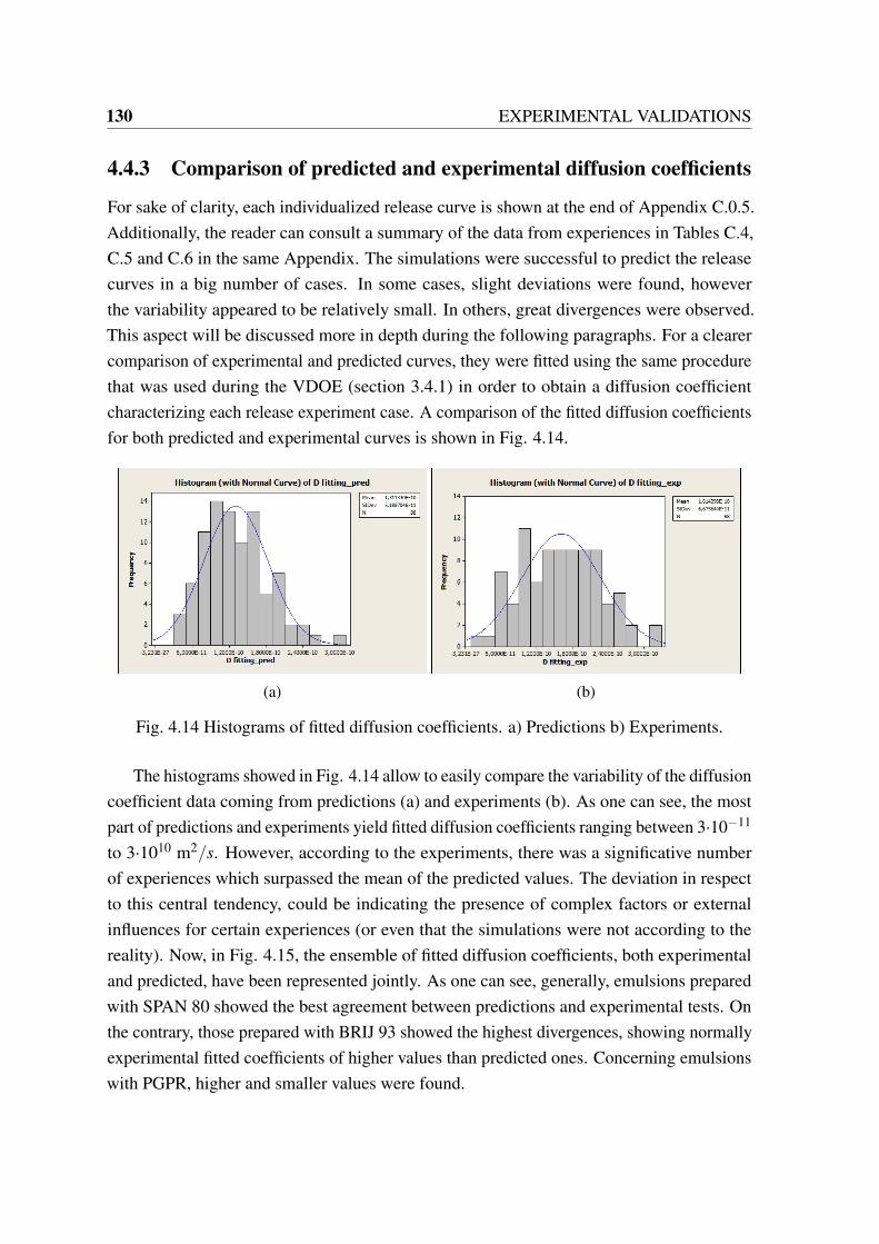
130 EXPERIMENTAL VALIDATIONS
4.4.3 Comparison of predicted and experimental diffusion coefficients
For sake of clarity, each individualized release curve is shown at the end of Appendix C.0.5.Additionally, the reader can consult a summary of the data from experiences in Tables C.4,C.5 and C.6 in the same Appendix. The simulations were successful to predict the releasecurves in a big number of cases. In some cases, slight deviations were found, howeverthe variability appeared to be relatively small. In others, great divergences were observed.This aspect will be discussed more in depth during the following paragraphs. For a clearercomparison of experimental and predicted curves, they were fitted using the same procedurethat was used during the VDOE (section 3.4.1) in order to obtain a diffusion coefficientcharacterizing each release experiment case. A comparison of the fitted diffusion coefficientsfor both predicted and experimental curves is shown in Fig. 4.14.
(a) (b)
Fig. 4.14 Histograms of fitted diffusion coefficients. a) Predictions b) Experiments.
The histograms showed in Fig. 4.14 allow to easily compare the variability of the diffusioncoefficient data coming from predictions (a) and experiments (b). As one can see, the mostpart of predictions and experiments yield fitted diffusion coefficients ranging between 3·10−11
to 3·1010 m2/s. However, according to the experiments, there was a significative numberof experiences which surpassed the mean of the predicted values. The deviation in respectto this central tendency, could be indicating the presence of complex factors or externalinfluences for certain experiences (or even that the simulations were not according to thereality). Now, in Fig. 4.15, the ensemble of fitted diffusion coefficients, both experimentaland predicted, have been represented jointly. As one can see, generally, emulsions preparedwith SPAN 80 showed the best agreement between predictions and experimental tests. Onthe contrary, those prepared with BRIJ 93 showed the highest divergences, showing normallyexperimental fitted coefficients of higher values than predicted ones. Concerning emulsionswith PGPR, higher and smaller values were found.

4.4 Predicted and experimental release experiments 131
(a) (b)
Fig. 4.15 a) Comparison of fitted diffusion coefficients of experimental curves versus pre-dicted ones. b) Comparison of fitted coefficient values per sample.
In Fig. 4.15b the value of these coefficients versus their respective identifying emulsionnumbers per experience have also been represented. In order to understand easily this graph,it is important to keep in mind that the first nine emulsion numbers represented for eachsystem (1-9, 31-39 and 61-69) are always referred to dodecane oil. Secondly, the followingnine points (10-18, 40-48, and 70-78) are referred to hexadecane oil. Then, with respect tothe final points, they are referred to myristate and palmitate oil in groups of six points eachone for SPAN 80 and PGPR systems, but in the case of BRIJ 93 systems, in groups of fivepoints only. This was like this because emulsions prepared using myristate and palmitate athighest dispersed phase volumetric fractions generally showed a noticeable instability andthey were dismissed for the release experiments.
However, the reader is invited to see clearer interpretations in the following boxplots ofFig. 4.16. Boxplots are powerful graphs, which provide a visual synopsis of the variationpatterns of the data distribution. The display consists of a rectangular box representingroughly the middle 50 % (interquartile range) of the data, and lines (’whiskers’) extending toeither side indicating the general extent of the data. It is also marked the median value insidethe box and the outliers. They are specially useful for this analysis since a high number ofdifferent data are being compared. As one can see, generally, a good agreement betweenpredicted and experimental curves was observed for emulsions prepared with dodecane orhexadecane oils when using SPAN 80 or PGPR as surfactants. However, deviations started tobecome important when myristate or palmitate oils where employed with these surfactants.On the other hand, when BRIJ 93 was employed, the deviations were more marked whenusing dodecane or hexadecane as oil. The greatest deviations from the whole study, speciallyoccured in release experiments from emulsions prepared with PGPR and BRIJ 93.

132 EXPERIMENTAL VALIDATIONS
(a) (b)
(c) (d)
(e) (f)
Fig. 4.16 Boxplots representing the variability of the fitted diffusion coefficients predicted(left) and experimental (right) of release experiments. They have been classified by surfactantand oil. a) and b) refer to SPAN 80 systems. c) and d) to PGPR systems. e) and f) to BRIJ 93systems.
After having compared the fitted diffusion coefficients as function of the surfactant andoil employed, some remarks will be done in the next section regarding these results in relationto the storage moduli.

4.4 Predicted and experimental release experiments 133
4.4.4 Analysis of storage moduli
As it was aforementioned, the storage moduli for each emulsion at the end of the releaseexperiment was measured. In the following Fig. 4.17 the relative errors concerning the changeof G’ (before and after release) as well as the relative errors concerning the fitted diffusioncoefficients (experimental and predicted) have been compared. Apparently, experimentswhich did not show significant differences on G’ (less than 20 %), were those experimentsgenerally related to a less deviation between the fitted diffusion coefficients. Since it istherefore likely that such connection exists, this kind of variations on G’ can indicate thatpossible structural changes are happening during the release. As a consequence, it could bethought that the model would not work correctly for predicting the release at these cases.
(a) (b)
(c)
Fig. 4.17 a) Relative errors in storage moduli (G’) before and after release. b) Relativeerrors between predicted Dpred. and experimental Dexp. diffusion coefficients (D). c) Jointlyrepresentation of relative errors concerning G’ and D.

134 EXPERIMENTAL VALIDATIONS
4.4.5 Model limitations and possible useful extensions
It is important to bear in mind that the mass transfer model developed, considers to keepconstant all its parameters. During the modeling, it was supposed that there was no variationof parameters with time or position. But when the emulsion releases the active ingredient,and even considering that the active ingredient is the only transferred component, someparameters such as the droplet diameter, the thickness of the emulsion placed in the containerand the dispersed phase mass fraction are likely going to decrease with time (even morerapidly if the emulsion was not stable).
The variation of time-dependent parameters may be complicated to incorporate in themass transfer model in order to build a more rigorous nonlinear ab-initio model, which willthen become it nonlinear. Nevertheless, this was not the objective of this thesis, since itwas decided to consider a simple model as general as possible. But even without havinga nonlinear model, it is however possible to assess the impact of some position-dependentand formulation parameters, for instance, by examination of the different release profiles atdecreasing dispersed phase mass fraction or thickness of emulsion layer.
(a) Variation of φm from 0.92 to 0.70 (b) Variation of thickness L [m]
Fig. 4.18 Examples of possible variations on release curve by time-dependent parameters.
As example, in Fig. 4.18a, variations caused by a decrease of the mass dispersed phasefraction are shown. More specifically, this simulation was the one corresponding to the mostextreme deviation detected in the SPAN 80 + Palmitate system (Emulsion No. 28). Allinput parameters for the ab-initio model were kept constant with the exception of the massdispersed phase fraction. As one can see, a decrease on this variable caused a rising on therelease curve. It could be conceivably hypothesized that in this specific case, this would beoccuring and was the reason for the deviation observed. Afterwards, in Fig. 4.18b it is shownhow a decrease on the thickness of the emulsion placed for the experiment could affect to the

4.4 Predicted and experimental release experiments 135
release profile. As one can see, the effect is not so notable in comparison with the change onthe dispersed phase mass fraction.
Some of these facts, individually or together with others, could have probably happenedduring the experimental release tests showing deviations. Specially, in some of the expe-riences showing a great divergence among predicted and experimental releases (typicallyemulsions using palmitate and myristate oils), it was visually remarked erosion-like effectson the surface of the remaining emulsions in the container at the end of the experiment. Inother cases, even a part of the emulsion could had been completely detached, or even in somecases, oil droplets were observed floating on the surface of the receptor solution. One of themost extreme cases was the emulsion No. 22 (See Fig. C.6g of Appendix C.0.5). In thisexperience, there was a variation of approximately 1500 Pa on G’ between the beginningand the end of the experience. During the initial times, a good agreement was achievedbetween predicted and experimental release curves, but as time increased, a divergence fromthe predicted profile started to appear, until arriving to the midpoint, where suddenly, a sharpincrease on the absorbance signal was observed.
Additionally, it is important to bear in mind, that the model do not adress the effectof possible enhancers or reducers which could modify the permeation, neither specificreactions of the active ingredient with other substances within the system, or even interactionsor association between the components. For example, the divergence between viscositymeasurements and the predictions performed by UNIFAC-VISCO, suggested that it could bepossibly hypothesized that more complex micelles structures could exist simultaneously inthe continuous media (limit of this approach). It is clear that this phenomena could take partin the mass transfer, and this fact might justify the specific deviations observed when usingPGPR as surfactant, specially the cases with a low deviation in G’. Other reasons could be animprecise estimation of molecular volume/area parameters, bearing in mind that the natureof this surfactant is polymeric-like. A possible useful extension for the ab-initio model couldbe to implement the effect of the micellar transport in the diffusion coefficient [183], in orderto correctly take into consideration this fact.
Given the limitations inherent to the model itself, as well as possibly uncertainty on theinputs or mass transport parameters dependent of emulsion composition such as distributioncoefficients predicted by UNIFAC, diffusion coefficients, molecular volumes/areas, perme-abilities, etc., the predictions in some cases could be only regarded as orientative values.Nevertheless, the findings were encouraging, and according to the satisfactory cases, we be-lieve that the model might be still capable of providing correct or at least first approximationswithin a low margin of error for a big number of cases.

136 EXPERIMENTAL VALIDATIONS
4.4.6 Screening of most accurate predicted scenarios
The predictions showing less experimental deviation to experimental fitted coefficients havebeen ploted and identified in Fig. 4.19. As one can see, checking the Table 4.1, equivalentcontrolled release profiles can be obtained using different formulations, o/s ratios or dispersedphase mass fractions. Therefore, the model allows to tune the emulsion properties in order toattain a given desired profile of active ingredient release.
Fig. 4.19 Predicted release profiles with less deviation error (ε ≈ 20%) in relation to ex-perimental tests. For the plot of these curves, Dfitting(pred.) and Dfitting(exp.) were usedrespectively in the exact analytical solution of Fick’s law. It is important to mention that thethickness of emulsion L was calculated according to weighted mass amount and can varyslightly between experiences.

4.4 Predicted and experimental release experiments 137
Table 4.1 Screening of predicted release curves with less experimental deviation error.
No. Oil Surfactant φm moil/msur f . Dfittingpred. Dfittingexp. ε (error)13 HEXADECANE SPAN 80 0.93 1.05 5.38E-11 4.60E-11 17.0129 PALMITATE SPAN 80 0.93 2.59 5.90E-11 6.67E-11 -11.4817 HEXADECANE SPAN 80 0.95 2.70 6.20E-11 5.49E-11 12.9110 HEXADECANE SPAN 80 0.91 1.06 6.88E-11 6.09E-11 13.0818 HEXADECANE SPAN 80 0.95 5.64 7.00E-11 6.85E-11 2.067 DODECANE SPAN 80 0.95 1.04 7.18E-11 6.47E-11 10.979 DODECANE SPAN 80 0.95 6.08 8.30E-11 9.08E-11 -8.58
14 HEXADECANE SPAN 80 0.93 2.43 8.31E-11 7.07E-11 17.568 DODECANE SPAN 80 0.95 2.93 8.83E-11 7.19E-11 22.87
27 PALMITATE SPAN 80 0.91 5.66 9.21E-11 1.08E-10 -14.8548 HEXADECANE PGPR 0.95 5.67 9.54E-11 1.10E-10 -13.024 DODECANE SPAN 80 0.93 1.06 1.01E-10 9.49E-11 5.99
76 HEXADECANE BRIJ 93 0.95 1.05 1.05E-10 9.20E-11 13.9511 HEXADECANE SPAN 80 0.91 2.64 1.13E-10 9.65E-11 17.135 DODECANE SPAN 80 0.93 2.50 1.24E-10 1.26E-10 -1.256 DODECANE SPAN 80 0.93 5.22 1.28E-10 1.33E-10 -4.111 DODECANE SPAN 80 0.91 1.10 1.28E-10 1.27E-10 1.23
12 HEXADECANE SPAN 80 0.91 5.65 1.30E-10 1.23E-10 4.9738 DODECANE PGPR 0.95 3.28 1.32E-10 1.13E-10 16.3366 DODECANE BRIJ 93 0.93 5.59 1.35E-10 1.67E-10 -18.8049 MYRISTATE PGPR 0.90 1.06 1.46E-10 1.84E-10 -20.5870 HEXADECANE BRIJ 93 0.93 1.00 1.55E-10 1.55E-10 0.0936 DODECANE PGPR 0.92 5.76 1.57E-10 1.72E-10 -8.723 DODECANE SPAN 80 0.91 5.48 1.63E-10 1.70E-10 -4.33
37 DODECANE PGPR 0.95 1.29 1.63E-10 1.33E-10 22.052 DODECANE SPAN 80 0.91 2.69 1.66E-10 1.66E-10 -0.19
63 DODECANE BRIJ 93 0.90 5.38 1.78E-10 2.24E-10 -20.5171 HEXADECANE BRIJ 93 0.91 2.62 1.81E-10 1.82E-10 -0.2842 HEXADECANE PGPR 0.90 5.38 1.90E-10 2.11E-10 -9.8435 DODECANE PGPR 0.92 2.57 1.93E-10 2.28E-10 -15.3462 DODECANE BRIJ 93 0.91 2.58 2.00E-10 1.97E-10 1.7840 HEXADECANE PGPR 0.90 1.05 2.02E-10 1.70E-10 18.7933 DODECANE PGPR 0.90 5.52 2.05E-10 2.27E-10 -9.8834 DODECANE PGPR 0.92 1.06 2.20E-10 1.96E-10 12.3461 DODECANE BRIJ 93 0.90 1.02 2.26E-10 2.24E-10 0.5251 MYRISTATE PGPR 0.87 5.45 2.37E-10 2.80E-10 -15.2532 DODECANE PGPR 0.90 2.72 2.53E-10 2.63E-10 -3.64

138 EXPERIMENTAL VALIDATIONS
4.4.7 Principal component analysis
Due to the complexity and the high number of parameters in the model, multivariate analysisprocedures to analyze the data are extremely suggested. Similar to the Pareto chart, aprincipal component analysis allows to reduce the data dimension, finding out the mostimportant variables and clear tendencies quickly. This is really interesting for reconciliationand intensification purposes, since it is possible to know the key variables (and respectiveweights) which most influence the response. Changes on these interrelated variables (principalcomponents) will assure changes on the targeted release profiles.
Fig. 4.20 Loading plot of principal component analysis. The study was done using allsimulation and experimental results and considering 25 components to be computed.
In order to analyze the data covariance structure, the principal component analysis wasperformed using the statitiscal software Minitab®. An overview of principal componentanalysis can be found in most books on multivariate analysis, such as [184]. A total numberof 25 components (variables) were chosen to compute in the analysis. The result of theloading plot for first two components is shown in Fig. 4.20. This plot checks the loadings forthe second principal component (y-axis) versus the scores for the first principal component (x-axis). A line is drawn from each loading to the (0,0) point. The similarity (lineal correlation)between variables can be interpreted from the graph. The closer the components ploted in

4.4 Predicted and experimental release experiments 139
the graph, the higher the possibilities of existing a lineal combination between them. Thenomenclature for the designation of the variables is the same that was employed in thelogical architecture diagram from section 3.2. A correlation matrix type was used becausethe variables were measured at different scales. In this way, the matrix makes sense in orderto standardize variables. In order to interpret the results of the principal component analysis,the screen plot and eigenanalysis of the correlation matrix are shown in Fig. 4.21.
Fig. 4.21 Screen plot of principal component analysis and values resulting from the eigen-analysis of the correlation matrix.
The first principal component has a variance (eigenvalue) 8.2794 and accounts for 33.1% of the total variance. The coefficients listed in Table 4.2 under PC1, allow to calculatethe principal component score (for instance, PC1=0.154·V1+0.246·V2-0.158·V3+...). Itshould be noted that the interpretation of the principal components is subjective, however,obvious patterns emerge quite often. For instance, because the weights of these terms haveopposite sign and are not close to zero, one could think of the first principal component asrepresenting an effect of the distribution coefficient Kcd and continuous phase viscosity (µc)to the effective diffusivity (De f f .) and global mass transfer coefficient (Kg). The secondprincipal component has variance 6.7176 and accounts for 60 % of the data variability. Thiscomponent could be thought of a contrasting level of the deposited surfactant amount on the

140 EXPERIMENTAL VALIDATIONS
interphase (msur f .), the interfacial area (Ainter f acial) and the monolayer thickness (∆s) withthe permeability of the surfactant layer (Ps) to some extent. For the third component PC3, asit was known beforehand from the Pareto chart, the dispersed phase mass fraction (φm) isclosely linked to the representative diffusion coefficients of the curves. In the forth, PC4, itis possible to see the relationship between the volume or thickness of the emulsion testedfor release (Vtotal and L respectively) with Ainter f acial and oil/surfactant ratio roil/sur f .. Inthe last principal component, PC5, the storage moduli (G’) appears to be specially relatedto φm and roil/sur f .. Together, first four and five components represent 81.8 % and 90.5 %,respectively, of the total variability. Thus, most of the data structure can be captured inthese five underlying dimensions instead. In following Figs. 4.22 to 4.23, different boxplotssummarize the values of these categorical variables.
Table 4.2 Weight coefficients of correlation matrix from principal component analysis.
Variable PC1 PC2 PC3 PC4 PC5V1 D f itting (exp.) 0.154 -0.048 -0.363 -0.189 0.081V2 D f itting (pred.) 0.246 0.087 -0.331 0.01 0.083V3 G’be f ore -0.158 0.232 0.033 -0.148 0.347V4 G’a f ter -0.154 0.237 -0.001 -0.124 0.332V5 roil/sur f . (real) 0.185 -0.107 0.188 -0.317 -0.331V6 roil/sur f . (preparation) 0.184 -0.116 0.174 -0.308 -0.344V7 Ddroplet 0.022 -0.291 0.231 0.065 0.06V8 φm -0.026 -0.139 0.44 0.108 0.303V9 φv -0.086 -0.162 0.362 0.108 0.362
V10 Ds 0.035 -0.308 -0.262 0.165 0.129V11 De f f . 0.321 -0.027 0.082 -0.04 0.216V12 Dc 0.326 -0.018 0.063 -0.044 0.199V13 BIOT 0.326 -0.018 0.063 -0.044 0.198V14 msur f .interphase 0.134 0.339 -0.025 0.079 0.025V15 ∆s 0.067 0.304 0.132 -0.286 0.115V16 A(inter f acial) 0.106 0.301 -0.025 0.306 -0.109V17 Vtotal 0.139 0.217 0.105 0.416 -0.137V18 L 0.139 0.217 0.105 0.416 -0.137V19 MWcont. -0.188 0.155 -0.173 -0.277 0.121V20 Kcd -0.264 -0.001 -0.237 0.177 0.13V21 Kg 0.324 0.055 -0.087 -0.018 0.109V22 kic 0.306 0.125 -0.08 -0.065 0.158V23 Pdis 0.074 -0.309 -0.21 0.121 0.091V24 µc -0.294 0.064 -0.043 -0.03 -0.103V25 Ps 0.075 -0.309 -0.21 0.121 0.092

4.4 Predicted and experimental release experiments 141
(a) (b)
(c) (d)
(e) (f)
Fig. 4.22 a) c) e) Boxplots representing the variability on distribution coefficients in theemulsions employed for release tests. b), d) and f) Boxplots representing the variability onviscosity [cP] of continuous phases predicted by UNIFAC-VISCO and used by the ab-initiomodel to perform the simulations.

142 EXPERIMENTAL VALIDATIONS
(a) (b)
(c) (d)
(e) (f)
Fig. 4.23 a) c) and d) Boxplots representing the variability on the estimated effective diffusioncoefficients [m2/s] of continuous phases (after applying the Maxwell relation) by the ab-initiomodel. b) d) and f) Boxplots representing the values of the global mass transfer coefficients[m/s] estimated on simulations.

4.4 Predicted and experimental release experiments 143
(a) (b)
(c) (d)
(e) (f)
Fig. 4.24 a) c) and d) Boxplots representing the variability on the calculated mass amounts ofsurfactant on the droplet surfaces. b) d) and f) Boxplots representing the variabilities of thecalculated surfactant layer permeabilities [cm/s].

144 EXPERIMENTAL VALIDATIONS
Some of the conclusions drawn from the multivariate analysis, as well as comments inregard to the representative key variables were:
• The principal component analysis demonstrated the key role of the interfacial film aswell as the partition coefficient of the diffusing molecule between the continuous andthe dispersed phase on the diffusion. Overall, faster release profiles were obtainedusing emulsions with low partition coefficients for the diffusing molecule and lowviscosities of continuous phase (see Fig. 4.22). It results interesting to note that evenif distribution coefficients were close for emulsions prepared with SPAN 80 BRIJ 93,the viscosities of continuous phases for SPAN 80 emulsions were generally muchhigher than those prepared with BRIJ 93. This appeared to have a special impact onthe release profile, giving slower diffusion rates. It can be thus suggested that theviscosity may not be negligible in terms of its impact on the diffusion coefficient:controlling the viscosity of the continuous media (for example by adding thickeners)could hypothetically lead to control slower releases.
• Regarding the estimated effective diffusion coefficient for the continuous phase, it wasobserved a direct and positive correlation with the global mass transfer coefficient.This fact confirmed again the importance of the dispersed phase mass fraction (as itwas already seen in the Pareto chart) when applying the Maxwell relation, since itsvalue determines to a great extent the order of the interfacial mass transfer coefficient.The higher this value, the less the resistance for the mass transfer (see Fig. 4.23).
• In some cases, it might be important to consider that surfactant permeabilities couldbe much greater than others and the interfacial resistance offered by the surfactantaround droplets would be extremely low (for instance, when using BRIJ 93). As aconsequence of this, generally faster release curves could be hypothetically obtained.However, with great permeabilities, caution must be applied, it may be the case thata rapid mass transfer through the surfactant layer could also lead to changes on thestructural parameters in a shorter time. This could cause subsequent instabilities, andprobably, is the reason that justifies the deviations observed between predictions andexperimental tests when using BRIJ 93 (see Fig. 4.24).
• It is also important to mention that the model is very sensitive to molecular parameterssuch as volumes or areas. More specifically, the ab-initio model calculates the thicknessof the emulsion (L) taking into account the respective molar volumes of the components.Any errors on inputs such as the weighted mass amount of emulsion for release or theoil/surfactant amounts could lead to strong miscalculations.

Chapter 5
FINAL CONCLUSIONS
’A great discovery solves a great problem, but there is a grain of discovery in the solution ofany problem. Your problem may be modest, but if it challenges your curiosity and brings intoplay your inventive faculties, and if you solve it by your own means, you may experience thetension and enjoy the triumph of discovery’, George Pólya.”
5.1 Summary of results and conclusions
In this thesis, a reverse engineering framework has been proposed to design and evaluatevehicles for controlled release of active ingredients. A convenience example of structured-dispersed system: highly concentrated emulsions, was considered. The design problem wasdecomposed into a hierachical sequence of subproblems or boxes (see Fig. 5.1), combining:
• Constitutive models, which estimate the active ingredient mass transport as a functionof formulation parameters, such as type of oil or surfactant, their mass ratio, emulsiondroplet diameter, active ingredient concentration, dispersed phase mass fraction, massemployed for the release experiment, as well as receptor solution volume.
• Computer-aided techniques, such as molecular modeling descriptors for estimationof volume/area of molecules, or group-contribution models employed for equilibriapredictions as well as for mixture viscosities estimations.
• Heuristic-based testing. Different simulation tools allowed to gain knowledge priorthe corresponding experimental validations concerning estimations of distributioncoefficients, mixture viscosities or the respective predicted release profiles.

146 FINAL CONCLUSIONS
Fig. 5.1 Work-flow diagram for a reverse engineering approach to design of controlled releaseproducts.
A summary of the most important aspects covered in the reverse engineering approach ofthis thesis, applied for highly concentrated emulsions, were the following:
• A programming code using three UNIFAC group-contribution methods (Fredenslund,Dortmund and Constantinescu) was written using MATLAB software in order to esti-mate activity coefficients of liquid-liquid mixtures. An additional flash algorithm basedon the Rachford and Rice equation was implemented for calculating the distributioncoefficients at equilibrium of active ingredient within the emulsion phases.
• Attemps to validate experimentally the above thermodynamic descriptors were per-formed by determination of distribution coefficients of emulsion-like samples byUV-spectrometry. However, these validations were limited in several ways. First, athree-phase system was observed for all samples and the experimental study was notable to take into account the third phase. Adding salt seemed to reduce the amount ofthis third phase, however, compensatory effects could be happening simultaneously,since UNIFAC methods, a priori, do not consider the presence of salts. Secondly,it was observed that possible microdroplets or microaggregates of oil or surfactantcould be misleading the UV-lecture because of interference effects. Although stocksolutions were employed as blank and dilution media for the samples measurement

5.1 Summary of results and conclusions 147
only slight improvements were achieved. In any case, the combinations of resultsprovided some support for the conceptual premise that the Modified UNIFAC methodof Contastinescu (2016) is the most suitable for predicting the distribution coefficientsfrom the three methods studied because of the better precisions obtained.
• Another programming code was written using MATLAB software to estimate thecontinuous phase mixture viscosities by UNIFAC-VISCO method. Experimentalvalidations were also performed to check the accuracy of the predictions. Overall, themethod appeared to yield estimations with good agreement between predicted andexperimental viscosities, with the exception of PGPR systems. In all other cases, lowdeviations were obtained, except cases of oil/surfactant ratios close to the unity.
• A full factorial design of virtual experiments has allowed to obtain a quantitativedescription of the release. These kind of sensitivity analysis, allowed to clearlyunderstand the main tendencies when changing the different formulation variablesprior performing any experiments. After, experimental kinetics validations have beenperformed.
The following conclusions can be drawn from the present thesis:
• It has been found that considering a limited cartography of 4 oils and 3 surfactants, theensemble of tools of the proposed reverse engineering approach, generally allowedto predict the temporal profiles of active ingredient (mandelic acid) release fromthe emulsions in the most part of cases. The results pointed in predicted releaseprofiles with representative Fickean diffusion coefficient values ranging from 3·10−11
to 3·10−10 m2/s (one order of magnitude).
• However, the success of the predictions were significantly limited to the emulsionstability. In spite of this fact, the mean absolute relative error between predicted andexperimental fitted diffusion coefficients for all release experiences performed (88experiences) was about a 16%.
• The application of this reverse engineering results very interesting regards intensifica-tion purposes and for the development of new controlled-delivery systems. Specially,because costly trial-and-error tests can be potentially avoided and the design can berationally facilitated when facing a set of existing possibilities.
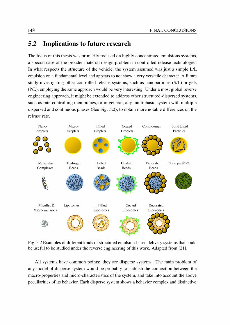
148 FINAL CONCLUSIONS
5.2 Implications to future research
The focus of this thesis was primarily focused on highly concentrated emulsions systems,a special case of the broader material design problem in controlled release technologies.In what respects the structure of the vehicle, the system assumed was just a simple L/Lemulsion on a fundamental level and appears to not show a very versatile character. A futurestudy investigating other controlled release systems, such as nanoparticles (S/L) or gels(P/L), employing the same approach would be very interesting. Under a most global reverseengineering approach, it might be extended to address other structured-dispersed systems,such as rate-controlling membranes, or in general, any multiphasic system with multipledispersed and continuous phases (See Fig. 5.2), to obtain more notable differences on therelease rate.
Fig. 5.2 Examples of different kinds of structured emulsion-based delivery systems that couldbe useful to be studied under the reverse engineering of this work. Adapted from [21].
All systems have common points: they are disperse systems. The main problem ofany model of disperse system would be probably to stablish the connection between themacro-properties and micro-characteristics of the system, and take into account the abovepeculiarities of its behavior. Each disperse system shows a behavior complex and distinctive.

5.2 Implications to future research 149
The inquiry that at any point could emerge is if a partition/diffusion description would beavailable or not to describe mass transfer in such more complex systems, or if specificinteractions (i.e. adsorption, reaction) or phenomena at nanoscale (molecular aggregates,such as micelles) would be expressly addressed. Nevertheless, even if each disperse systempossesses their own thermodynamic properties and characteristics, one expects under a reverseengineering approach that each system could be hypothetically explained by including thespecific content on the adequate box.
Fig. 5.3 Schematics of the computer program system used to generate, solve and verify themathematical models of a given structured-dispersed system. Adapted from [22].
Therefore, the forward problem, which involves the computation of a controlled releasefor a given product would appear to be solved. However, it is also important to remind thatthe choice of a delivery system, rather must be driven by the nature of the active ingredientwithin its application domain, and the inherent properties of the respective release systems.Properties of the active ingredient, including chemistry, solubility, etc., influence on theproper selection of a desired delivery system that can achieve the desired outcomes. It isrequired thus, to rely on a suitable cartography database of different and adequate dispersesystems (depending on the domain of application), which would allow to see significativedifferences or effects on the release rate.
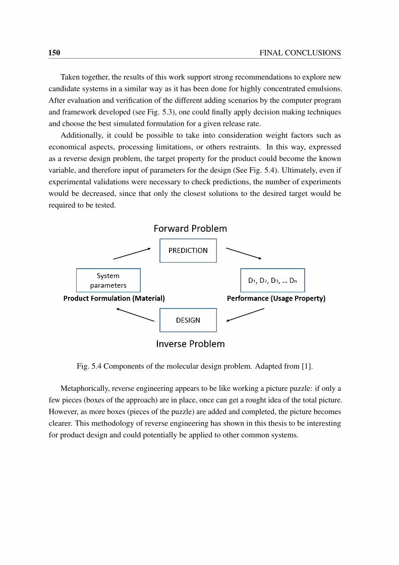
150 FINAL CONCLUSIONS
Taken together, the results of this work support strong recommendations to explore newcandidate systems in a similar way as it has been done for highly concentrated emulsions.After evaluation and verification of the different adding scenarios by the computer programand framework developed (see Fig. 5.3), one could finally apply decision making techniquesand choose the best simulated formulation for a given release rate.
Additionally, it could be possible to take into consideration weight factors such aseconomical aspects, processing limitations, or others restraints. In this way, expressedas a reverse design problem, the target property for the product could become the knownvariable, and therefore input of parameters for the design (See Fig. 5.4). Ultimately, even ifexperimental validations were necessary to check predictions, the number of experimentswould be decreased, since that only the closest solutions to the desired target would berequired to be tested.
Fig. 5.4 Components of the molecular design problem. Adapted from [1].
Metaphorically, reverse engineering appears to be like working a picture puzzle: if only afew pieces (boxes of the approach) are in place, once can get a rought idea of the total picture.However, as more boxes (pieces of the puzzle) are added and completed, the picture becomesclearer. This methodology of reverse engineering has shown in this thesis to be interestingfor product design and could potentially be applied to other common systems.

5.2 Implications to future research 151
Fig.
5.5
Met
apho
rica
lpuz
zle
repr
esen
tatio
nof
reve
rse
engi
neer
ing
appr
oach
.


References
[1] LEK Achenie, R Gani, and V Venkatasubramanian. Genetic algorithms based camd.Computer Aided Molecular Design: Theory and Practice, 12:95, 2002.
[2] Jinhyun Hannah Lee and Yoon Yeo. Controlled drug release from pharmaceuticalnanocarriers. Chemical engineering science, 125:75–84, 2015.
[3] Jennifer R Weiser and W Mark Saltzman. Controlled release for local delivery ofdrugs: barriers and models. Journal of Controlled Release, 190:664–673, 2014.
[4] Agnieszka Kowalczuk, Roza Trzcinska, Barbara Trzebicka, Axel HE Müller, An-drzej Dworak, and Christo B Tsvetanov. Loading of polymer nanocarriers: factors,mechanisms and applications. Progress in Polymer Science, 39(1):43–86, 2014.
[5] Nily Dan. Transport and release in nano-carriers for food applications. Journal ofFood Engineering, 175:136–144, 2016.
[6] Martien A Cohen Stuart, Wilhelm TS Huck, Jan Genzer, Marcus Müller, ChristopherOber, Manfred Stamm, Gleb B Sukhorukov, Igal Szleifer, Vladimir V Tsukruk, MarekUrban, et al. Emerging applications of stimuli-responsive polymer materials. Naturematerials, 9(2):101–113, 2010.
[7] David O Cooney. Effect of geometry on the dissolution of pharmaceutical tablets andother solids: surface detachment kinetics controlling. AIChE Journal, 18(2):446–449,1972.
[8] Junichi Takahara, Kozo Takayama, and Tsuneji Nagai. Multi-objective simultaneousoptimization technique based on an artificial neural network in sustained releaseformulations. Journal of controlled release, 49(1):11–20, 1997.
[9] J Siepmann and F Siepmann. Mathematical modeling of drug delivery. Internationaljournal of pharmaceutics, 364(2):328–343, 2008.
[10] Juergen Siepmann and Florence Siepmann. Modeling of diffusion controlled drugdelivery. Journal of Controlled Release, 161(2):351–362, 2012.
[11] Paolo Colombo, Ruggero Bettini, and Nikolaos A Peppas. Observation of swellingprocess and diffusion front position during swelling in hydroxypropyl methyl cellulose(hpmc) matrices containing a soluble drug. Journal of Controlled Release, 61(1):83–91, 1999.

154 References
[12] Richard W Korsmeyer, Steven R Lustig, and Nikolaos A Peppas. Solute and penetrantdiffusion in swellable polymers. i. mathematical modeling. Journal of Polymer SciencePart B: Polymer Physics, 24(2):395–408, 1986.
[13] PI Lee. Diffusional release of a solute from a polymeric matrix—approximate analyti-cal solutions. Journal of membrane science, 7(3):255–275, 1980.
[14] Juergen Siepmann, Nathalie Faisant, and Jean-Pierre Benoit. A new mathematicalmodel quantifying drug release from bioerodible microparticles using monte carlosimulations. Pharmaceutical Research, 19(12):1885–1893, 2002.
[15] David Julian McClements. Advances in fabrication of emulsions with enhancedfunctionality using structural design principles. Current Opinion in Colloid & InterfaceScience, 17(5):235–245, 2012.
[16] Fernando P Bernardo and Pedro M Saraiva. A theoretical model for transdermaldrug delivery from emulsions and its dependence upon formulation. Journal ofpharmaceutical sciences, 97(9):3781–3809, 2008.
[17] R Farajzadeh, R Krastev, and Pacelli LJ Zitha. Foam film permeability: Theory andexperiment. Advances in colloid and interface science, 137(1):27–44, 2008.
[18] Dana Constantinescu and Jürgen Gmehling. Addendum to “further development ofmodified unifac (dortmund): Revision and extension 6”. Journal of Chemical &Engineering Data, 62(7):2230–2230, 2017.
[19] Fernando Barragán-Aroche and Enrique Bazúa-Rueda. Estrategias de convergenciapara equilibrio líquido-líquido. el problema del" flash" negativo.
[20] Lutz Weber. Jchem base-chemaxon, 2008.
[21] David Julian McClements and Yan Li. Structured emulsion-based delivery systems:Controlling the digestion and release of lipophilic food components. Advances incolloid and interface science, 159(2):213–228, 2010.
[22] G Halász, T Virág, J Gyenis, T Blickle, and Z Csapó. Computer-aided generation ofmathematical models of steady-state heat and mass transfer processes. Computers &Chemical Engineering, 3(1-4):519–521, 1979.
[23] Christianto Wibowo and Ka M Ng. Product-centered processing: Manufacture ofchemical-based consumer products. AIChE Journal, 48(6):1212–1230, 2002.
[24] NA Peppas. Analysis of fickian and non-fickian drug release from polymers. 1985.
[25] Yuan H Zhao, Michael H Abraham, and Andreas M Zissimos. Fast calculation of vander waals volume as a sum of atomic and bond contributions and its application todrug compounds. The Journal of organic chemistry, 68(19):7368–7373, 2003.
[26] Bruce E Poling, John M Prausnitz, John P O’connell, et al. The properties of gasesand liquids, volume 5. Mcgraw-hill New York, 2001.

References 155
[27] Jürgen Gmehling, Jiding Li, and Martin Schiller. A modified unifac model. 2. presentparameter matrix and results for different thermodynamic properties. Industrial &Engineering Chemistry Research, 32(1):178–193, 1993.
[28] Dana Constantinescu and Jürgen Gmehling. Further development of modified unifac(dortmund): Revision and extension 6. Journal of Chemical & Engineering Data,61(8):2738–2748, 2016.
[29] Elliot J. Chikofsky and James H Cross. Reverse engineering and design recovery: Ataxonomy. IEEE software, 7(1):13–17, 1990.
[30] Hugo Bruneliere, Jordi Cabot, Grégoire Dupé, and Frédéric Madiot. Modisco: Amodel driven reverse engineering framework. Information and Software Technology,56(8):1012–1032, 2014.
[31] Eldad Eilam. Reversing: secrets of reverse engineering. John Wiley & Sons, 2011.
[32] R Costa, GD Moggridge, and PM Saraiva. Chemical product engineering: an emergingparadigm within chemical engineering. AIChE Journal, 52(6):1976–1986, 2006.
[33] E Favre, L Marchal-Heusler, and M Kind. Chemical product engineering: researchand educational challenges. Chemical Engineering Research and Design, 80(1):65–74,2002.
[34] Rafiqul Gani, Kim Dam-Johansen, and Ka M Ng. Chemical product design: A briefoverview. Chemical product design: toward a perspective through case studies, 2006.
[35] Guennadi M Ostrovsky, Luke EK Achenie, and Manish Sinha. On the solution ofmixed-integer nonlinear programming models for computer aided molecular design.Computers & chemistry, 26(6):645–660, 2002.
[36] Jens Abildskov and GM Kontogeorgis. Chemical product design: A new challenge ofapplied thermodynamics. Chemical Engineering Research and Design, 82(11):1505–1510, 2004.
[37] JM Prausnitz. Thermodynamics and the other chemical engineering sciences: oldmodels for new chemical products and processes. Fluid phase equilibria, 158:95–111,1999.
[38] Fernando P Bernardo and Pedro M Saraiva. Value of information analysis in prod-uct/process design. Computer Aided Chemical Engineering, 18:151–156, 2004.
[39] Ignacio E Grossmann. Challenges in the new millennium: product discovery anddesign, enterprise and supply chain optimization, global life cycle assessment. Com-puters & Chemical Engineering, 29(1):29–39, 2004.
[40] Gary Blau, Bharat Mehta, Shantanu Bose, Joe Pekny, Gavin Sinclair, Kay Keunker,and Paul Bunch. Risk management in the development of new products in highlyregulated industries. Computers & Chemical Engineering, 24(2-7):659–664, 2000.
[41] Christos T Maravelias and Ignacio E Grossmann. Simultaneous planning for newproduct development and batch manufacturing facilities. Industrial & engineeringchemistry research, 40(26):6147–6164, 2001.
156 References
[42] Dharmashankar Subramanian, Joseph F Pekny, Gintaras V Reklaitis, and Gary EBlau. Simulation-optimization framework for stochastic optimization of r&d pipelinemanagement. AIChE Journal, 49(1):96–112, 2003.
[43] Anna Kogan and Nissim Garti. Microemulsions as transdermal drug delivery vehicles.Advances in colloid and interface science, 123:369–385, 2006.
[44] Kinam Park. Controlled drug delivery systems: past forward and future back. Journalof Controlled Release, 190:3–8, 2014.
[45] Ronald A Siegel and Michael J Rathbone. Overview of controlled release mechanisms.In Fundamentals and Applications of Controlled Release Drug Delivery, pages 19–43.Springer, 2012.
[46] Sara A Abouelmagd, Hyesun Hyun, and Yoon Yeo. Extracellularly activatable nanocar-riers for drug delivery to tumors. Expert opinion on drug delivery, 11(10):1601–1618,2014.
[47] Miles C Braithwaite, Charu Tyagi, Lomas K Tomar, Pradeep Kumar, Yahya EChoonara, and Viness Pillay. Nutraceutical-based therapeutics and formulation strate-gies augmenting their efficiency to complement modern medicine: An overview.Journal of Functional Foods, 6:82–99, 2014.
[48] Eric Dickinson and Martin E Leser. Food colloids: self-assembly and material science,volume 308. Royal Society of chemistry, 2007.
[49] Inteaz Alli Catherine N. Mulligan Bernard F. Gibbs, Selim Kermasha. Encapsulationin the food industry: a review. International journal of food sciences and nutrition,50(3):213–224, 1999.
[50] John N Coupland and John E Hayes. Physical approaches to masking bitter taste:lessons from food and pharmaceuticals. Pharmaceutical research, 31(11):2921–2939,2014.
[51] Mahmoud Elsabahy and Karen L Wooley. Design of polymeric nanoparticles forbiomedical delivery applications. Chemical Society Reviews, 41(7):2545–2561, 2012.
[52] Hua Wei, Ren-Xi Zhuo, and Xian-Zheng Zhang. Design and development of polymericmicelles with cleavable links for intracellular drug delivery. Progress in polymerScience, 38(3):503–535, 2013.
[53] Jeffrey A Hubbell and Ashutosh Chilkoti. Nanomaterials for drug delivery. Science,337(6092):303–305, 2012.
[54] Ru Cheng, Fenghua Meng, Chao Deng, Harm-Anton Klok, and Zhiyuan Zhong. Dualand multi-stimuli responsive polymeric nanoparticles for programmed site-specificdrug delivery. Biomaterials, 34(14):3647–3657, 2013.
[55] Jianbin Tang, Yuqi Sheng, Hongjie Hu, and Youqing Shen. Macromolecular mricontrast agents: structures, properties and applications. Progress in Polymer Science,38(3):462–502, 2013.

References 157
[56] Tennyson L Doane and Clemens Burda. The unique role of nanoparticles innanomedicine: imaging, drug delivery and therapy. Chemical Society Reviews,41(7):2885–2911, 2012.
[57] Joaquim Miguel Oliveira, António José Salgado, Nuno Sousa, João Filipe Mano,and Rui Luís Reis. Dendrimers and derivatives as a potential therapeutic tool inregenerative medicine strategies—a review. Progress in Polymer Science, 35(9):1163–1194, 2010.
[58] Jae Hyung Park, Seulki Lee, Jong-Ho Kim, Kyeongsoon Park, Kwangmeyung Kim,and Ick Chan Kwon. Polymeric nanomedicine for cancer therapy. Progress in PolymerScience, 33(1):113–137, 2008.
[59] M Talha Gokmen and Filip E Du Prez. Porous polymer particles—a comprehensiveguide to synthesis, characterization, functionalization and applications. Progress inpolymer science, 37(3):365–405, 2012.
[60] Mikhail Motornov, Yuri Roiter, Ihor Tokarev, and Sergiy Minko. Stimuli-responsivenanoparticles, nanogels and capsules for integrated multifunctional intelligent systems.Progress in polymer science, 35(1):174–211, 2010.
[61] Robert Langer and Nikolaos Peppas. Chemical and physical structure of polymers ascarriers for controlled release of bioactive agents: a review. Journal of MacromolecularScience-Reviews in Macromolecular Chemistry and Physics, 23(1):61–126, 1983.
[62] Simon Herrlich, Sven Spieth, Stephan Messner, and Roland Zengerle. Osmoticmicropumps for drug delivery. Advanced drug delivery reviews, 64(14):1617–1627,2012.
[63] NA Peppas, P Bures, Ws Leobandung, and H Ichikawa. Hydrogels in pharmaceuticalformulations. European journal of pharmaceutics and biopharmaceutics, 50(1):27–46,2000.
[64] Chien-Chi Lin and Andrew T Metters. Hydrogels in controlled release formula-tions: network design and mathematical modeling. Advanced drug delivery reviews,58(12):1379–1408, 2006.
[65] Ping I Lee. Novel approach to zero-order drug delivery via immobilized nonuni-form drug distribution in glassy hydrogels. Journal of pharmaceutical sciences,73(10):1344–1347, 1984.
[66] Santanu Kaity, Jinu Isaac, and Animesh Ghosh. Interpenetrating polymer network oflocust bean gum-poly (vinyl alcohol) for controlled release drug delivery. Carbohy-drate polymers, 94(1):456–467, 2013.
[67] Soo Hyeon Lee, Hyejung Mok, Yuhan Lee, and Tae Gwan Park. Self-assembledsirna–plga conjugate micelles for gene silencing. Journal of controlled release,152(1):152–158, 2011.

158 References
[68] Mani Prabaharan, Jamison J Grailer, Srikanth Pilla, Douglas A Steeber, and ShaoqinGong. Amphiphilic multi-arm-block copolymer conjugated with doxorubicin via ph-sensitive hydrazone bond for tumor-targeted drug delivery. Biomaterials, 30(29):5757–5766, 2009.
[69] Hyuk Sang Yoo and Tae Gwan Park. Biodegradable polymeric micelles composedof doxorubicin conjugated plga–peg block copolymer. Journal of controlled Release,70(1):63–70, 2001.
[70] Friederike von Burkersroda, Luise Schedl, and Achim Göpferich. Why degradablepolymers undergo surface erosion or bulk erosion. Biomaterials, 23(21):4221–4231,2002.
[71] Wen-Chuan Lee, I Chu, et al. Preparation and degradation behavior of polyanhydridesnanoparticles. Journal of Biomedical Materials Research Part B: Applied Biomaterials,84(1):138–146, 2008.
[72] Susanne Fredenberg, Marie Wahlgren, Mats Reslow, and Anders Axelsson. Themechanisms of drug release in poly (lactic-co-glycolic acid)-based drug deliverysystems—a review. International journal of pharmaceutics, 415(1):34–52, 2011.
[73] Jindrich Kopecek. Controlled biodegradability of polymers—a key to drug deliverysystems. Biomaterials, 5(1):19–25, 1984.
[74] Scott H Medina, Maxim V Chevliakov, Gopinath Tiruchinapally, Yasemin YukselDurmaz, Sibu P Kuruvilla, and Mohamed EH ElSayed. Enzyme-activated nanocon-jugates for tunable release of doxorubicin in hepatic cancer cells. Biomaterials,34(19):4655–4666, 2013.
[75] Kyung Hyun Min, Jong-Ho Kim, Sang Mun Bae, Hyeri Shin, Min Sang Kim, SangjinPark, Hyejung Lee, Rang-Woon Park, In-San Kim, Kwangmeyung Kim, et al. Tu-moral acidic ph-responsive mpeg-poly (β -amino ester) polymeric micelles for cancertargeting therapy. Journal of Controlled Release, 144(2):259–266, 2010.
[76] Cong Chang, Hua Wei, Chang-Yun Quan, Yong-Yong Li, Jia Liu, Zong-Chun Wang,Si-Xue Cheng, Xian-Zheng Zhang, and Ren-Xi Zhuo. Fabrication of thermosensitivepcl-pnipaam-pcl triblock copolymeric micelles for drug delivery. Journal of PolymerScience Part A: Polymer Chemistry, 46(9):3048–3057, 2008.
[77] J Siepmann and NA Peppas. Modeling of drug release from delivery systems basedon hydroxypropyl methylcellulose (hpmc). Advanced drug delivery reviews, 48(2-3):139–157, 2001.
[78] J Siepmann and A Göpferich. Mathematical modeling of bioerodible, polymeric drugdelivery systems. Advanced drug delivery reviews, 48(2):229–247, 2001.
[79] Davis Yohanes Arifin, Lai Yeng Lee, and Chi-Hwa Wang. Mathematical modeling andsimulation of drug release from microspheres: implications to drug delivery systems.Advanced drug delivery reviews, 58(12):1274–1325, 2006.
[80] T Higuchi. Physical chemical analysis of percutaneous absorption process fromcreams and ointments. J. Soc. Cosmet. Chem, 11:85–97, 1960.

References 159
[81] Takeru Higuchi. Rate of release of medicaments from ointment bases containing drugsin suspension. Journal of pharmaceutical sciences, 50(10):874–875, 1961.
[82] J Siepmann, A Ainaoui, JM Vergnaud, and R Bodmeier. Calculation of the dimensionsof drug–polymer devices based on diffusion parameters. Journal of pharmaceuticalsciences, 87(7):827–832, 1998.
[83] Balaji Narasimhan. Mathematical models describing polymer dissolution: conse-quences for drug delivery. Advanced Drug Delivery Reviews, 48(2):195–210, 2001.
[84] Göran Frenning and Maria Strømme. Drug release modeled by dissolution, diffusion,and immobilization. International journal of pharmaceutics, 250(1):137–145, 2003.
[85] V Lemaire, J Belair, and P Hildgen. Structural modeling of drug release frombiodegradable porous matrices based on a combined diffusion/erosion process. Inter-national journal of pharmaceutics, 258(1):95–107, 2003.
[86] Y Zhou and XY Wu. Modeling and analysis of dispersed-drug release into a finitemedium from sphere ensembles with a boundary layer. Journal of controlled release,90(1):23–36, 2003.
[87] Göran Frenning, Ulrika Brohede, and Maria Strømme. Finite element analysis ofthe release of slowly dissolving drugs from cylindrical matrix systems. Journal ofcontrolled release, 107(2):320–329, 2005.
[88] Chandrashekar Raman, Cory Berkland, Kyekyoon Kevin Kim, and Daniel W Pack.Modeling small-molecule release from plg microspheres: effects of polymer degrada-tion and nonuniform drug distribution. Journal of Controlled Release, 103(1):149–158,2005.
[89] Philip L Ritger and Nikolaos A Peppas. A simple equation for description of soluterelease i. fickian and non-fickian release from non-swellable devices in the form ofslabs, spheres, cylinders or discs. Journal of controlled release, 5(1):23–36, 1987.
[90] Philip L Ritger and Nikolaos A Peppas. A simple equation for description of soluterelease ii. fickian and anomalous release from swellable devices. Journal of controlledrelease, 5(1):37–42, 1987.
[91] HB Hopfenberg. Controlled release from erodible slabs, cylinders, and spheres. ACSPublications, 1976.
[92] Yixin Chen, Troy W McCall, Anand R Baichwal, and Marvin C Meyer. The applicationof an artificial neural network and pharmacokinetic simulations in the design ofcontrolled-release dosage forms. Journal of controlled release, 59(1):33–41, 1999.
[93] Svetlana Ibric, Milica Jovanovic, Zorica Djuric, Jelena Parojcic, and Ljiljana Solomun.The application of generalized regression neural network in the modeling and opti-mization of aspirin extended release tablets with eudragit® rs po as matrix substance.Journal of Controlled Release, 82(2):213–222, 2002.

160 References
[94] Abdollahi Ghaffari, H Abdollahi, MR Khoshayand, I Soltani Bozchalooi, A Dadgar,and M Rafiee-Tehrani. Performance comparison of neural network training algo-rithms in modeling of bimodal drug delivery. International journal of pharmaceutics,327(1):126–138, 2006.
[95] Qun Shao, Raymond C Rowe, and Peter York. Comparison of neurofuzzy logicand neural networks in modelling experimental data of an immediate release tabletformulation. European journal of pharmaceutical sciences, 28(5):394–404, 2006.
[96] Emmanuelle Cauchetier, M Deniau, H Fessi, A Astier, and M Paul. Atovaquone-loadednanocapsules: influence of the nature of the polymer on their in vitro characteristics.International journal of pharmaceutics, 250(1):273–281, 2003.
[97] John Crank. The mathematics of diffusion. Oxford university press, 1979.
[98] Richard William Baker et al. Controlled release of biologically active agents. JohnWiley & Sons, 1987.
[99] Per Borgquist, Gunnar Zackrisson, Bernt Nilsson, and Anders Axelsson. Simulationand parametric study of a film-coated controlled-release pharmaceutical. Journal ofcontrolled release, 80(1):229–245, 2002.
[100] Jean-Maurice Vergnaud. Controlled drug release of oral dosage forms. CRC Press,1993.
[101] T Higuchi. Mechanism of sustained-action medication. theoretical analysis of rate ofrelease of solid drugs dispersed in solid matrices. Journal of pharmaceutical sciences,52(12):1145–1149, 1963.
[102] Liang-tseng Fan and Satish K Singh. Controlled release: A quantitative treatment,volume 13. Springer Science & Business Media, 2012.
[103] E Doelker. Water-swollen cellulose derivatives in pharmacy. Hydrogels in medicineand pharmacy, 2:115–160, 1987.
[104] Hiroshi Fujita. Diffusion in polymer-diluent systems. Fortschritte Der Hochpolymeren-Forschung, pages 1–47, 1961.
[105] Robert TC Ju, Phillip R Nixon, Mahesh V Patel, and Donald M Tong. Drug releasefrom hydrophilic matrices. 2. a mathematical model based on the polymer disentan-glement concentration and the diffusion layer. Journal of pharmaceutical sciences,84(12):1464–1477, 1995.
[106] J Siepmann and NA Peppas. Hydrophilic matrices for controlled drug delivery:an improved mathematical model to predict the resulting drug release kinetics (the“sequential layer” model). Pharmaceutical Research, 17(10):1290–1298, 2000.
[107] Balaji Narasimhan, Nikolaos A Peppas, et al. Disentanglement and reptation duringdissolution of rubbery polymers. Journal of Polymer Science-B-Polymer PhysicsEdition, 34(5):947–962, 1996.

References 161
[108] Kyriacos Zygourakis and Pauline A Markenscoff. Computer-aided design of bio-erodible devices with optimal release characteristics: a cellular automata approach.Biomaterials, 17(2):125–135, 1996.
[109] N Faisant, J Siepmann, J Richard, and JP Benoit. Mathematical modeling of drugrelease from bioerodible microparticles: effect of gamma-irradiation. EuropeanJournal of Pharmaceutics and Biopharmaceutics, 56(2):271–279, 2003.
[110] Jean Bézivin. On the unification power of models. Software and Systems Modeling,4(2):171–188, 2005.
[111] Elisa Conte, Rafiqul Gani, and Ka Ming Ng. Design of formulated products: asystematic methodology. AIChE journal, 57(9):2431–2449, 2011.
[112] Jens M Sørensen, Thomas Magnussen, Peter Rasmussen, and Aage Fredenslund.Liquid—liquid equilibrium data: Their retrieval, correlation and prediction part ii:Correlation. Fluid Phase Equilibria, 3(1):47–82, 1979.
[113] Meritxell Llinàs, Gabriela Calderó, M José García-Celma, Alessandro Patti, andConxita Solans. New insights on the mechanisms of drug release from highly concen-trated emulsions. Journal of colloid and interface science, 394:337–345, 2013.
[114] Gabriela Calderó, Meritxell Llinàs, María José García-Celma, and Conxita Solans.Studies on controlled release of hydrophilic drugs from w/o high internal phase ratioemulsions. Journal of pharmaceutical sciences, 99(2):701–711, 2010.
[115] H Maekawa, Jordi Esquena, Samuel Bishop, Conxita Solans, and Bradley F Chmelka.Meso/macroporous inorganic oxide monoliths from polymer foams. Advanced Mate-rials, 15(7-8):591–596, 2003.
[116] Laia Espelt, Pere Clapés, Jordi Esquena, Albert Manich, and Conxita Solans. Enzy-matic carbon- carbon bond formation in water-in-oil highly concentrated emulsions(gel emulsions). Langmuir, 19(4):1337–1346, 2003.
[117] Nina S Nielsen, Arni Petersen, Anne S Meyer, Maike Timm-Heinrich, and CharlotteJacobsen. Effects of lactoferrin, phytic acid, and edta on oxidation in two food emul-sions enriched with long-chain polyunsaturated fatty acids. Journal of agriculturaland food chemistry, 52(25):7690–7699, 2004.
[118] AP Guimarães, DAS Maia, RS Araújo, CL Cavalcante Jr, and HB de Sant’Ana.Destabilization and recuperability of oil used in the formulation of concentratedemulsions and cutting fluids. Chemical and Biochemical Engineering Quarterly,24(1):43–49, 2010.
[119] Carin Malmborg, Daniel Topgaard, and Olle Söderman. Nmr diffusometry and theshort gradient pulse limit approximation. Journal of Magnetic Resonance, 169(1):85–91, 2004.
[120] Justin Ashworth, Elisabeth J Wurtmann, and Nitin S Baliga. Reverse engineeringsystems models of regulation: discovery, prediction and mechanisms. Current opinionin biotechnology, 23(4):598–603, 2012.

162 References
[121] Edward Lansing Cussler. Diffusion: mass transfer in fluid systems. Cambridgeuniversity press, 2009.
[122] RP Borwankar, CC Chan, DT Wasan, RM Kurzeja, ZM Gu, and NN Li. Analysis ofthe effect of internal phase leakage on liquid membrane separations. AIChE journal,34(5):753–762, 1988.
[123] Linda R De Young and Ken A Dill. Solute partitioning into lipid bilayer membranes.Biochemistry, 27(14):5281–5289, 1988.
[124] Samir Mitragotri, Mark E Johnson, Daniel Blankschtein, and Robert Langer. Ananalysis of the size selectivity of solute partitioning, diffusion, and permeation acrosslipid bilayers. Biophysical journal, 77(3):1268–1283, 1999.
[125] Tian-Xiang Xiang and Bradley D Anderson. Permeability of acetic acid across geland liquid-crystalline lipid bilayers conforms to free-surface-area theory. Biophysicaljournal, 72(1):223–237, 1997.
[126] Abdel-Halim Ghanem, WI Higuchi, and AP Simonelli. Interfacial barriers in inter-phase transport: Retardation of the transport of diethylphthalate across the hexadecane-water interface by an adsorbed gelatin film. Journal of pharmaceutical sciences,58(2):165–174, 1969.
[127] Stephanie R Dungan, Beverly H Tai, and Natalia I Gerhardt. Transport mechanisms inthe micellar solubilization of alkanes in oil-in-water emulsions. Colloids and SurfacesA: Physicochemical and Engineering Aspects, 216(1):149–166, 2003.
[128] CR Wilke and Pin Chang. Correlation of diffusion coefficients in dilute solutions.AIChE Journal, 1(2):264–270, 1955.
[129] Johannes Lyklema. Fundamentals of interface and colloid science: soft colloids,volume 5. Academic press, 2005.
[130] Aage Fredenslund, Russell L Jones, and John M Prausnitz. Group-contribution estima-tion of activity coefficients in nonideal liquid mixtures. AIChE Journal, 21(6):1086–1099, 1975.
[131] A Bondi. Physical properties of molecular liquids, crystals and glasses. Wlley: NewYork, 1968.
[132] Henrik K Hansen, Peter Rasmussen, Aage Fredenslund, Martin Schiller, and JürgenGmehling. Vapor-liquid equilibria by unifac group contribution. 5. revision andextension. Industrial & Engineering Chemistry Research, 30(10):2352–2355, 1991.
[133] Josef P Novák, Jaroslav Matouš, and Jirí Pick. Liquid-liquid equilibria, volume 7.Elsevier Science Ltd, 1987.
[134] Zhigang Lei, Biaohua Chen, Chengyue Li, and Hui Liu. Predictive molecular thermo-dynamic models for liquid solvents, solid salts, polymers, and ionic liquids. Chemicalreviews, 108(4):1419–1455, 2008.

References 163
[135] I Kikic, P Alessi, Peter Rasmussen, and Aage Fredenslund. On the combinatorial partof the unifac and uniquac models. The Canadian Journal of Chemical Engineering,58(2):253–258, 1980.
[136] Eugene R Thomas and Charles A Eckert. Prediction of limiting activity coefficientsby a modified separation of cohesive energy density model and unifac. Industrial &Engineering Chemistry Process Design and Development, 23(2):194–209, 1984.
[137] Jürgen Lohmann, Ralph Joh, and Jürgen Gmehling. From unifac to modified unifac(dortmund). Industrial & engineering chemistry research, 40(3):957–964, 2001.
[138] Jürgen Gmehling, Jürgen Lohmann, Antje Jakob, Jiding Li, and Ralph Joh. A mod-ified unifac (dortmund) model. 3. revision and extension. Industrial & engineeringchemistry research, 37(12):4876–4882, 1998.
[139] Jürgen Gmehling, Roland Wittig, Jürgen Lohmann, and Ralph Joh. A modified unifac(dortmund) model. 4. revision and extension. Industrial & engineering chemistryresearch, 41(6):1678–1688, 2002.
[140] Antje Jakob, Hans Grensemann, Jürgen Lohmann, and Jürgen Gmehling. Furtherdevelopment of modified unifac (dortmund): revision and extension 5. Industrial &engineering chemistry research, 45(23):7924–7933, 2006.
[141] Andreas Zuend and John H Seinfeld. A practical method for the calculation ofliquid–liquid equilibria in multicomponent organic–water–electrolyte systems usingphysicochemical constraints. Fluid Phase Equilibria, 337:201–213, 2013.
[142] Lee E Baker, Alan C Pierce, Kraemer D Luks, et al. Gibbs energy analysis of phaseequilibria. Society of Petroleum Engineers Journal, 22(05):731–742, 1982.
[143] HH Rachford Jr, JD Rice, et al. Procedure for use of electronic digital computersin calculating flash vaporization hydrocarbon equilibrium. Journal of PetroleumTechnology, 4(10):19–3, 1952.
[144] Curtis H Whitson and Michael L Michelsen. The negative flash. Fluid Phase Equilib-ria, 53:51–71, 1989.
[145] John M Prausnitz. Computer calculations for multicomponent vapor-liquid andliquid-liquid equilibria. Prentice Hall, 1980.
[146] Viviana Consonni, Roberto Todeschini, and Manuela Pavan. Structure/responsecorrelations and similarity/diversity analysis by getaway descriptors. 1. theory of thenovel 3d molecular descriptors. Journal of Chemical Information and ComputerSciences, 42(3):682–692, 2002.
[147] John Bruce Irving. Viscosity of binary liquid mixtures: a survey of mixture equations.National Engineering Laboratory, 1977.
[148] Y Gaston-Bonhomme, P Petrino, and JL Chevalier. Unifac—visco group contributionmethod for predicting kinematic viscosity: extension and temperature dependence.Chemical engineering science, 49(11):1799–1806, 1994.

164 References
[149] JL Chevalier, P Petrino, and Y Gaston-Bonhomme. Estimation method for the kine-matic viscosity of a liquid-phase mixture. Chemical engineering science, 43(6):1303–1309, 1988.
[150] MT Tyn and WF Calus. Estimating liquid molal volume. Processing, 21(4):16–17,1975.
[151] Aksel L Lydersen and Madison Engineering Experiment Station. Estimation of criticalproperties of organic compounds by the method of group contributions. University ofWisconsin, 1955.
[152] Kevin G Joback. A unified approach to physical property estimation using multivariatestatistical techniques. PhD thesis, Massachusetts Institute of Technology, 1984.
[153] Kevin G Joback and Robert C Reid. Estimation of pure-component properties fromgroup-contributions. Chemical Engineering Communications, 57(1-6):233–243, 1987.
[154] Charalambos G Varelas, David G Dixon, and Carol A Steiner. Mathematical model ofmass transport through dispersed-phase polymer networks. AIChE Journal, 41(4):805–811, 1995.
[155] Charalambos G Varelas, David G Dixon, and Carol A Steiner. Zero-order release frombiphasic polymer hydrogels. Journal of controlled release, 34(3):185–192, 1995.
[156] Mario Grassi, Gabriele Grassi, Romano Lapasin, and Italo Colombo. Understandingdrug release and absorption mechanisms: A physical and mathematical approach.CRC Press, 2006.
[157] Jens T Carstensen. Modeling and data treatment in the pharmaceutical sciences. CRCPress, 1996.
[158] Paolo Freguglia. Modelli matematici nelle scienze biologiche, 1998.
[159] R Gani, LEK Achenie, and V Venkatasubramanian. Introduction to camd. 2003.
[160] Renata M Debowska, Aleksandra Kaszuba, Iwona Michalak, Agata Dzwigałowska,Czanita Ciescinska, Elzbieta Jakimiuk, Joanna Zielinska, and Andrzej Kaszuba. Evalu-ation of the efficacy and tolerability of mandelic acid-containing cosmetic formulationsfor acne skin care. Dermatology Review/Przeglad Dermatologiczny, 102(3), 2015.
[161] Frank H Clarke and Natalie M Cahoon. Ionization constants by curve fitting: Deter-mination of partition and distribution coefficients of acids and bases and their ions.Journal of pharmaceutical sciences, 76(8):611–620, 1987.
[162] G Calderó, MJ García-Celma, C Solans, and R Pons. Effect of ph on mandelic aciddiffusion in water in oil highly concentrated emulsions (gel-emulsions). Langmuir,16(4):1668–1674, 2000.
[163] David S Wishart, Craig Knox, An Chi Guo, Roman Eisner, Nelson Young, Bijaya Gau-tam, David D Hau, Nick Psychogios, Edison Dong, Souhaila Bouatra, et al. Hmdb: aknowledgebase for the human metabolome. Nucleic acids research, 37(suppl_1):D603–D610, 2008.

References 165
[164] Michael P Aronson and Michael F Petko. Highly concentrated water-in-oil emulsions:Influence of electrolyte on their properties and stability. Journal of colloid andinterface science, 159(1):134–149, 1993.
[165] Adnan Azeem, Zeenat Iqbal Khan, M Aqil, Farhan Jalees Ahmad, Roop Kishan Khar,and Sushama Talegaonkar. Microemulsions as a surrogate carrier for dermal drugdelivery. Drug development and industrial pharmacy, 35(5):525–547, 2009.
[166] High Production Volume HPV Challenge and EPA All. Federal register notice;voluntary children’s chemical evaluation program.
[167] Myristyl Myristate. Final report on the safety assessment of myristyl myristate andisopropyl myristate. J Am Coll Toxicol, 1:55–80, 1982.
[168] Mahesh V Patel and Feng-Jing Chen. Solid carriers for improved delivery of activeingredients in pharmaceutical compositions, June 19 2001. US Patent 6,248,363.
[169] C Hinton. Alkoxylated nonionic surfactants. chapter: 3. The Chemistry and Manufac-ture of Cosmetics, 3:15–27, 2002.
[170] Andrea Saltelli, Marco Ratto, Terry Andres, Francesca Campolongo, Jessica Cariboni,Debora Gatelli, Michaela Saisana, and Stefano Tarantola. Global sensitivity analysis:the primer. John Wiley & Sons, 2008.
[171] David J Pannell. Sensitivity analysis of normative economic models: theoreticalframework and practical strategies. Agricultural economics, 16(2):139–152, 1997.
[172] A Bahremand and F De Smedt. Distributed hydrological modeling and sensitivityanalysis in torysa watershed, slovakia. Water Resources Management, 22(3):393–408,2008.
[173] Mary C Hill, Dmitri Kavetski, Martyn Clark, Ming Ye, Mazdak Arabi, Dan Lu, LauraFoglia, and Steffen Mehl. Practical use of computationally frugal model analysismethods. Groundwater, 54(2):159–170, 2016.
[174] Mary C Hill and Claire R Tiedeman. Effective groundwater model calibration: withanalysis of data, sensitivities, predictions, and uncertainty. John Wiley & Sons, 2006.
[175] Michael J Berry and Gordon Linoff. Data mining techniques: for marketing, sales,and customer support. John Wiley & Sons, Inc., 1997.
[176] Donald W Marquardt. An algorithm for least-squares estimation of nonlinear parame-ters. Journal of the society for Industrial and Applied Mathematics, 11(2):431–441,1963.
[177] Jorge J Moré. The levenberg-marquardt algorithm: implementation and theory. InNumerical analysis, pages 105–116. Springer, 1978.
[178] Tapash K Ghosh and Bhaskara R Jasti. Theory and practice of contemporary pharma-ceutics. CRC press, 2004.
[179] Leland Wilkinson. Revising the pareto chart. The American Statistician, 60(4):332–334, 2006.

166 References
[180] Jean-Louis Salager, RE Antón, José Maria Anderez, and Jean-Marie Aubry. Formula-tion des micro-émulsions par la méthode hld. Techniques de l’Ingénieur, 157:2001,2001.
[181] Suwimon Ariyaprakai and Stephanie R Dungan. Contribution of molecular path-ways in the micellar solubilization of monodisperse emulsion droplets. Langmuir,24(7):3061–3069, 2008.
[182] Emilio Paruta-Tuarez, Hala Fersadou, Véronique Sadtler, Philippe Marchal, LionelChoplin, Christophe Baravian, and Christophe Castel. Highly concentrated emulsions:1. average drop size determination by analysis of incoherent polarized steady lighttransport. Journal of colloid and interface science, 346(1):136–142, 2010.
[183] Wyatt J Musnicki, Stephanie R Dungan, and Ronald J Phillips. Multicomponentdiffusion in solute-containing micelle and microemulsion solutions. Langmuir,30(37):11019–11030, 2014.
[184] Harry H Harman. Modern factor analysis. University of Chicago Press, 1976.

Appendix A
UNIFAC parameters for modelingactivity coefficients
UNIFAC (Revision and Extension 5) Hansen et al (1991)Modified UNIFAC (Dortmund) (Revision and Extension 2) Gmehling et al (1993)Modified UNIFAC (Dortmund) (Revision and Extension 6) Constantinescu et Gmehling (2016)

168 UNIFAC parameters for modeling activity coefficientsTa
ble
A.1
Gro
upSp
ecifi
catio
nsan
dSa
mpl
eG
roup
Ass
ignm
ents
forU
NIF
AC
Met
hod
(Han
sen,
etal
.199
1).P
art(
1/4)
.Tak
enfr
om[2
6].
Sam
ple
Ass
ignm
ents
Gro
upnu
mbe
r=
(Num
bero
fOcu
rren
ces)×
Seco
ndar
yM
ain
Rk
Qk
Nam
e(S
econ
dary
Gro
upN
umbe
r)1
1C
H3
0.90
110.
848
Hex
ane
=(2
)(1)
+(4
)(2)
12
CH
20.
6744
0.54
2-M
ethy
lpro
pane
=(3
)(1)
+(1
)(3)
13
CH
0.44
690.
228
Neo
pent
ane
=(4
)(1)
+(1
)(4)
14
C0.
2195
02,
2,4-
Trim
ethy
lpen
tane
=(5
)(1)
+(1
)(2)
+(1
)(3)
+(1
)(4)
25
CH
2=C
H1.
3454
1.17
63-
Met
hyl-
1-he
xene
=(2
)(1)
+(2
)(2)
+(1
)(3)
+(1
)(5)
26
CH
=CH
1.11
670.
867
Hex
ene-
2=
(2)(
1)+
(2)(
2)+
(1)(
6)2
7C
H2=
C1.
1173
0.98
82-
Met
hyl-
1-bu
tene
=(2
)(1)
+(1
)(2)
+(1
)(7)
28
CH
=C0.
8886
0.67
62-
Met
hyl-
2-bu
tene
=(3
)(1)
+(1
)(8)
270
C=C
0.66
050.
485
2,3-
Dim
ethy
lbut
ene
=(4
)(1)
+(1
)(70
)3
9A
CH
0.53
130.
4B
enze
ne=
(6)(
9)3
10A
C0.
3652
0.12
Styr
ene
=(1
)(5)
+(5
)(9)
+(1
)(10
)4
11A
CC
H3
1.26
630.
968
Tolu
ene
=(5
)(9)
+(1
)(11
)4
12A
CC
H2
1.03
960.
66E
thyl
benz
ene
=(1
)(1)
+(5
)(9)
+(1
)(12
)4
13A
CC
H0.
8121
0.34
8C
umen
e=
(2)(
1)+
(5)(
9)+
(1)(
13)
514
OH
11.
2E
than
ol=
(1)(
1)+
(1)(
2)+
(1)(
14)
615
CH
3OH
1.43
111.
432
Met
hano
l=(1
)(15
)7
16H
2O0.
921.
4W
ater
=(1
)(16
)8
17A
CO
H0.
8952
0.68
Phen
ol=
(5)(
9)+
(1)(
17)
918
CH
3CO
1.67
241.
488
Met
hyle
thyl
keto
ne=
(1)(
1)+
(1)(
2)+
(1)(
18)
919
CH
2CO
1.44
571.
18E
thyl
phen
ylke
tone
=(1
)(1)
+(1
)(19
)+(5
)(9)
+(1
)(10
)10
20C
HO
0.99
80.
948
Hex
anal
=(1
)(1)
+(4
)(2)
+(1
)(20
)11
21C
H3C
OO
1.90
311.
728
But
ylac
etat
e=
(1)(
1)+
(3)(
2)+
(1)(
21)
1122
CH
2CO
O1.
6764
1.42
Met
hylp
ropi
onat
e=
(2)(
1)+
(1)(
22)
1223
HC
OO
1.24
21.
188
Eth
ylfo
rmat
e=
(1)(
1)+
(1)(
2)+
(1)(
23)

169Ta
ble
A.2
UN
IFA
CM
etho
d(H
anse
n,et
al.1
991)
.Par
t(2/
4).T
aken
from
[26]
.
Gro
upnu
mbe
rVo
lum
eA
rea
Sam
ple
Ass
ignm
ents
=(N
umbe
rofO
curr
ence
s)×
Seco
ndar
yM
ain
Rk
Qk
Nam
e(S
econ
dary
Gro
upN
umbe
r)13
24C
H3O
1.14
51.
088
Dim
ethy
leth
er=
(1)(
1)+
(1)(
24)
1325
CH
2O0.
9183
0.78
Die
thyl
ethe
r=(2
)(1)
+(1
)(2)
+(1
)(25
)13
26C
HO
0.69
080.
468
Diis
opro
pyle
ther
=(4
)(1)
+(1
)(3)
+(1
)(26
)13
27T
HF
0.91
831.
1Te
trah
ydro
fura
n=
(3)(
2)+
(1)(
27)
1428
CH
3NH
21.
5959
1.54
4M
ethy
lam
ine
=(1
)(28
)14
29C
H2N
H2
1.36
921.
236
Eth
ylam
ine
=(1
)(1)
+(1
)(29
)14
30C
HN
H2
1.14
170.
924
Isop
ropy
lam
ine
=(2
)(1)
+(1
)(30
)15
31C
H3N
H1.
4337
1.24
4D
imet
hyla
min
e=
(1)(
1)+
(1)(
31)
1532
CH
2NH
1.20
70.
936
Die
thyl
amin
e=
(2)(
1)+
(1)(
2)+
(1)(
32)
1533
CH
NH
0.97
950.
624
Diis
opro
pyla
min
e=
(4)(
1)+
(1)(
3)+
(1)(
33)
1634
CH
3N1.
1865
0.94
Trim
ethy
lam
ine
=(2
)(1)
+(1
)(34
)16
35C
H2N
0.95
970.
632
Trie
thyl
amin
e=
(3)(
1)+
(2)(
2)+
(1)(
35)
1736
AC
NH
21.
060.
816
Ani
line
=(5
)(9)
+(1
)(36
)18
37C
5H5N
2.99
932.
113
Pyri
dine
=(1
)(37
)18
38C
5H4N
2.83
321.
833
2-M
ethy
lpyr
idin
e=
(1)(
1)+
(1)(
38)
1839
C5H
3N2.
667
1.55
32,
3-D
imet
hylp
yrid
ine
=(2
)(1)
+(1
)(39
)19
40C
H3C
N1.
8701
1.72
4A
ceto
nitr
ile=
(1)(
40)
1941
CH
2CN
1.64
341.
416
Prop
rion
itrile
=(1
)(1)
+(1
)(41
)20
42C
OO
H1.
3013
1.22
4A
cetic
Aci
d=
(1)(
1)+
(1)(
42)
2043
HC
OO
H1.
528
1.53
2Fo
rmic
Aci
d=
(1)(
43)
2144
CH
2Cl
1.46
541.
264
1-C
hlor
obut
ane
=(1
)(1)
+(2
)(2)
+(1
)(44
)21
45C
HC
l1.
238
0.95
22-
Chl
orop
ropa
ne=
(2)(
1)+
(1)(
45)
2146
CC
l1.
0106
0.72
42-
Chl
oro-
2-m
ethy
lpro
pane
=(3
)(1)
+(1
)(46
)22
47C
H2C
l 22.
2564
1.98
8D
ichl
orom
etha
ne=
(1)(
47)
2248
CH
Cl 2
2.06
061.
684
1,1-
Dic
hlor
oeth
ane
=(1
)(1)
+(1
)(48
)22
49C
Cl 2
1.80
161.
448
2,2-
Dic
hlor
opro
pane
=(2
)(1)
+(1
)(49
)23
50C
HC
l 32.
872.
41C
hlor
ofor
m=
(1)(
50)
2351
CC
l 32.
6401
2.18
41,
1,1-
Tric
hlor
oeth
ane
=(1
)(1)
+(1
)(51
)

170 UNIFAC parameters for modeling activity coefficientsTa
ble
A.3
UN
IFA
CM
etho
d(H
anse
n,et
al.1
991)
.Par
t(3/
4).T
aken
from
[26]
.
Gro
upnu
mbe
rVo
lum
eA
rea
Sam
ple
Ass
ignm
ents
=(N
umbe
rofO
curr
ence
s)×
Seco
ndar
yM
ain
Rk
Qk
Nam
e(S
econ
dary
Gro
upN
umbe
r)24
52C
Cl 4
3.39
2.91
Tetr
achl
orom
etha
ne=
(1)(
52)
2553
AC
Cl
1.15
620.
844
Chl
orob
enze
ne=
(5)(
9)+
(1)(
53)
2654
CH
3NO
22.
0086
1.86
8N
itrom
etha
ne=
(1)(
54)
2655
CH
2NO
21.
7818
1.56
Nitr
oeth
ane
=(1
)(1)
+(1
)(55
)26
56C
HN
O2
1.55
441.
248
2-N
itrop
ropa
ne=
(2)(
1)+
(1)(
56)
2757
AC
NO
21.
4199
1.10
4N
itrob
enze
ne=
(5)(
9)+
(1)(
57)
2858
CS 2
2.50
71.
65C
arbo
ndi
sulfi
de=
(1)(
58)
2959
CH
3SH
1.87
71.
676
Met
hane
thio
l=(1
)(59
)29
60C
H2S
H1.
651
1.36
8E
than
ethi
ol=
(1)(
1)+
(1)(
60)
3263
I1.
264
0.99
2Io
doet
hane
=(1
)(1)
+(1
)(2)
+(1
)(63
)33
64B
r0.
9492
0.83
2B
rom
oeth
ane
=(1
)(1)
+(1
)(2)
+(1
)(64
)34
65C
H=C
1.29
291.
088
1-H
exyn
e=
(1)(
1)+
(3)(
2)+
(1)(
65)
3466
C=C
1.06
130.
784
2-H
exyn
e=
(2)(
1)+
(2)(
2)+
(1)(
66)
3567
DM
SO2.
8266
2.47
2D
imet
hyls
ulfo
xide
=(1
)(67
)36
68A
cryl
onitr
ile2.
3144
2.05
2A
cryl
onitr
ile=
(1)(
68)
3769
Cl-
(C=C
)0.
791
0.72
4Tr
ichl
oroe
thyl
ene
=(1
)(8)
+(3
)(69
)38
71A
CF
0.69
480.
524
Fluo
robe
nzen
e=
(5)(
9)+
(1)(
71)
3972
DM
F3.
0856
2.73
6N
,N-D
imet
hylf
orm
amid
e=
(1)(
72)
3973
HC
ON
(CH
2)2
2.63
222.
12N
,N-D
ieth
ylfo
rmam
ide
=(2
)(1)
+(1
)(73
)40
74C
F 31.
406
1.38
Perfl
uoro
etha
ne=
(2)(
74)
4075
CF 2
1.01
050.
9240
76C
F0.
0615
0.46
Perfl
uoro
met
hylc
yclo
hexa
ne=(
1)(7
4)+
(5)(
75)+
(1)(
76)
4177
CO
O1.
381.
2B
utyl
acet
ate
=(2
)(1)
+(3
)(2)
+(1
)(77
)42
78Si
H3
1.60
351.
263
Met
hyls
ilane
=(1
)(1)
+(1
)(78
)42
79Si
H2
1.44
431.
006
Die
thyl
sila
ne=
(2)(
1)+
(2)(
2)+
(1)(
79)
4280
SiH
1.28
530.
749
Trim
ethy
lsila
ne=
(3)(
1)+
(1)(
80)
4281
Si1.
047
0.41
Tetr
amet
hyls
ilane
=(4
)(1)
+(1
)(81
)

171Ta
ble
A.4
UN
IFA
CM
etho
d(H
anse
n,et
al.1
991)
.Par
t(4/
4).T
aken
from
[26]
.
Gro
upnu
mbe
rVo
lum
eA
rea
Sam
ple
Ass
ignm
ents
=(N
umbe
rofO
curr
ence
s)×
Seco
ndar
yM
ain
Rk
Qk
Nam
e(S
econ
dary
Gro
upN
umbe
r)43
82Si
H2O
1.48
381.
062
4383
SiH
O1.
303
0.76
443
84Si
O1.
1044
0.46
6H
exam
ethy
ldis
iloxa
ne=
(6)(
1)+
(1)(
81)+
(1)(
84)
4485
NM
P3.
981
3.2
N-M
ethy
lpyr
rolid
one
=(1
)(85
)45
86C
Cl 3
F3.
0356
2.64
4Tr
icho
loro
fluor
omet
hane
=(1
)(86
)45
87C
Cl 2
F2.
2287
1.91
6Te
trac
hlor
o-1,
2-di
fluor
oeth
ane
=(2
)(87
)45
88H
CC
l 2F
2.40
62.
116
Dic
hlor
ofluo
rom
etha
ne=
(1)(
88)
4589
HC
ClF
1.64
931.
416
2-C
hlor
o-2-
fluor
oeth
ane
=(1
)(1)
+(1
)(89
)45
90C
ClF
21.
8174
1.64
82-
Chl
oro-
2,2-
diflu
oroe
than
e=
(1)(
1)+
(1)(
90)
4591
HC
ClF
21.
967
1.82
8C
holo
rodi
fluor
omet
hane
=(1
)(91
)45
92C
ClF
32.
721
2.1
Cho
loro
trifl
uoro
met
hane
=(1
)(92
)45
93C
Cl 2
F 22.
6243
2.37
6D
icho
loro
diflu
orom
etha
ne=
(1)(
93)
4694
CO
NH
21.
4515
1.24
8A
ceta
mid
e=
(1)(
1)+
(1)(
94)
4695
CO
NH
CH
32.
1905
1.79
6N
-Met
hyla
ceta
mid
e=
(1)(
1)+
(1)(
95)
4696
CO
NH
CH
21.
9637
1.48
8N
-Eth
ylac
etam
ide
=(2
)(1)
+(1
)(96
)46
97C
ON
(CH
3)2
2.85
892.
428
N,N
-Dim
ethy
lace
tam
ide
=(1
)(1)
+(1)
(97)
4698
CO
N(C
H3)
CH
22.
6322
2.12
N,N
-Met
hyle
thyl
acet
amid
e=
(2)(
1)+(
1)(9
8)46
99C
ON
(CH
2)2
2.40
541.
812
N,N
-Die
thyl
acet
amid
e=
(3)(
1)+(
1)(9
9)47
100
C2H
5O2
2.12
261.
904
2-E
thox
yeth
anol
=(1
)(1)
+(1)
(100
)47
101
C2H
4O2
1.89
521.
592
2-E
thox
y-1-
prop
anol
=(2
)(1)
+(1
)(2)
+(1
)(10
1)48
102
CH
3S1.
613
1.36
8D
imet
hyls
ulfid
e=
(1)(
1)+
(1)(
102)
4810
3C
H2S
1.38
631.
06D
ieth
ylsu
lfide
=(2
)(1)
+(1
)(2)
+(1
)(10
3)48
104
CH
S1.
1589
0.74
8D
iisop
ropy
lsul
fide
=(4
)(1)
+(1
)(3)
+(1
)(10
4)49
105
MO
RPH
3.47
42.
796
Mor
phol
ine
=(1
)(10
5)49
106
C4H
4S2.
8569
2.14
Thi
ophe
ne=
(1)(
106)
4910
7C
4H3S
2.69
081.
862-
Met
hylth
ioph
ene
=(1
)(1)
+(1
)(10
7)49
108
C4H
2S2.
5247
1.58
2-D
imet
hylth
ioph
ene
=(2
)(1)
+(1
)(10
8)

172 UNIFAC parameters for modeling activity coefficients
Table A.5 Rk and Qk Parameters and Group Assignment for Modified UNIFAC (Dortmund)Method. Gmehling et al (1993). Part (1/2) Taken from [27].
Group Volume AreaSecondary Main Rk Qk Name Example
1 1 0.6325 1.0608 CH3 hexane2 1 0.6325 0.7081 CH2 octane3 1 0.6325 0.3554 CH 2-methylpropane4 1 0.6325 0 C neopentane5 2 1.2832 1.6016 CH2=CH 1-hexene6 2 1.2832 1.2489 CH=CH 2-hexene7 2 1.2832 1.2489 CH2=C 2-methyl-1-butene8 2 1.2832 0.8962 CH=C 2-methyl-2-butene
70 2 1.2832 0.4582 C=C 2,3-dimethyl-2-b utene9 3 0.3763 0.4321 ACH naphthalene
10 3 0.3763 0.2113 AC styrene11 4 0.91 0.949 ACCH3 toluene12 4 0.91 0.7962 ACCH2 ethylbenzene13 4 0.91 0.3769 ACCH isopropylbenzene14 5 1.2302 0.8927 OH (p) 1-propanol81 5 1.063 0.8663 OH (s) 2-propanol82 5 0.6895 0.8345 OH (t) tert-butanol15 6 0.8585 0.9938 CH3OH methanol16 7 1.7334 2.4561 H2O water17 8 1.08 0.975 ACOH phenol18 9 1.7048 1.67 CH3CO 2-butanone19 9 1.7048 1.5542 CH2CO 2-pentanone20 10 0.7173 0.771 CHO propionic aldhyde21 11 1.27 1.6286 CH3COO butyl acetate22 11 1.27 1.4228 CH2COO methyl propionate23 12 1.9 1.8 HCOO ethyl formate24 13 1.1434 1.6022 CH3O dimethyl ether25 13 1.1434 1.2495 CH2O diethyl ether26 13 1.1434 0.8968 CHO diisopropyl ether28 14 1.6607 1.6904 CH3NH2 methylamine29 14 1.6607 1.3377 CH2NH2 ethylamine30 14 1.6607 0.985 CHNH2 isopropylamine85 14 1.6607 0.985 CNH2 tert-butylamine31 15 1.368 1.4332 CH3NH dimethylamine32 15 1.368 1.0805 CH2NH diethylamine33 15 1.368 0.7278 CHNH diisopropylamine34 16 1.0746 1.176 CH3N trimethylamine35 16 1.0746 0.824 CH2N triethylamine36 17 1.1849 0.8067 ACNH2 aniline37 18 2.5 2.1477 C5H5N pyridine38 18 2.8882 2.2496 C5H4N 2-methylpyridine39 18 3.2211 2.5 C5H3N 2,3-dimethylpyridine

173
Table A.6 Rk and Qk Parameters and Group Assignment for the Modified UNIFAC (Dort-mund) Method. Gmehling et al (1993). Part (2/2). Taken from [27].
Group Volume AreaSecondary Main Rk Qk Name Example
40 19 1.5575 1.5193 CH3CN acetonitrile41 19 1.5575 1.1666 CH2CN propionitrile42 20 0.8 0.9215 COOH acetic acid44 21 0.9919 1.3654 CH2Cl 1-chlorobutane45 21 0.9919 1.0127 CHCl 2-chloropropane46 21 0.9919 0.66 CCl tert-butyl chloride47 22 1.8 2.5 CH2Cl2 dichloromethane48 22 1.8 2.1473 CHCl2 1,l-dichloroethane49 22 1.8 1.7946 CCl2 2,2-dichloropropane51 23 2.65 2.3778 CCl3 l,l,l-trichloroethane52 24 2.618 3.1836 CCl4 tetrachloromethane53 25 0.5365 0.3177 ACCl chlorobenzene54 26 2.644 2.5 CH3NO2 nitromethane55 26 2.5 2.304 CH2NO2 1-nitropropane56 26 2.887 2.241 CHNO2 2-nitropropane57 27 0.4656 0.3589 ACNO2 nitrobenzene58 28 1.24 1.068 CS2 carbon disulfide59 29 1.289 1.762 CH3SH methanethiol60 29 1.535 1.316 CH2SH ethanethiol61 30 1.299 1.289 furfural furfural62 31 2.088 2.4 DOH 1,2-ethanediol63 32 1.076 0.9169 I ethyl iodide64 33 1.209 1.4 Br ethyl bromide65 34 0.9214 1.3 CH≡C 1-hexyne66 34 1.303 1.132 C≡C 2-hexyne67 35 3.6 2.692 DMSO dimethyl sulfoxide68 36 1 0.92 acrylonitrile acrylonitrile69 37 0.5229 0.7391 Cl(C≡C) trichloroethylene71 38 0.8814 0.7269 ACF hexafluorobenzene72 39 2 2.093 DMF NJ-dimethylformamide73 39 2.381 1.522 HCON(CH2)2 NJ-diethylformamide74 40 1.284 1.266 CF3 l,l,l-trifluoroethane75 40 1.284 1.098 CF2 perfluorohexane76 40 0.8215 0.5135 CF perfluoromethylcyclohexane77 41 1.6 0.9 COO methyl acrylate78 42 0.7136 0.8635 c-CH2 cyclohexane79 42 0.3479 0.1071 c-CH methylcyclohexane80 42 0.347 0 c-C 1,1-dimethylcyclohexane27 43 1.7023 1.8784 c-CH2OCH2 tetrahydrofuran83 43 1.4046 1.4 c-CH2O[CH2]1/2 1,3-dioxane84 43 1.0413 1.0116 c-[CH2O]1/2O[CH2]1/2 1,3,5-trioxane43 44 0.8 1.2742 HCOOH formic acid50 45 2.45 2.8912 CHCl3 chloroform

174 UNIFAC parameters for modeling activity coefficients
Table A.7 Rk and Qk Parameters and Group Assignment for Modified UNIFAC (Dortmund)Method. Constantinescu et Gmehling (2016). Part (1/3). Taken from Addendum to “FurtherDevelopment of Modified UNIFAC (Dortmund): Revision and Extension 6. [28].
Group Volume AreaSecondary Main Rk Qk Name Example
1 1 0.6325 1.0608 CH3 hexane2 1 0.6325 0.7081 CH2 octane3 1 0.6325 0.3554 CH 2-methylpropane4 1 0.6325 0 C neopentane5 2 1.2832 1.6016 CH2=CH 1-hexene6 2 1.2832 1.2489 CH=CH 2-hexene7 2 1.2832 1.2489 CH2=C 2-methyl-1-butene8 2 1.2832 0.8962 CH=C 2-methyl-2-butene
70 2 1.2832 0.4582 C=C 2,3-dimethyl-2-butene9 3 0.3763 0.4321 ACH naphthalene
10 3 0.3763 0.2113 AC styrene11 4 0.91 0.949 ACCH3 toluene12 4 0.91 0.7962 ACCH2 ethylbenzene13 4 0.91 0.3769 ACCH isopropylbenzene14 5 1.2302 0.8927 OH (p) 1-propanol81 5 1.063 0.8663 OH (s) 2-propanol82 5 0.6895 0.8345 OH (t) tert-butanol15 6 0.8585 0.9938 CH3OH methanol16 7 1.7334 2.4561 H2O water17 8 1.08 0.975 ACOH phenol18 9 1.7048 1.67 CH3CO 2-butanone19 9 1.7048 1.5542 CH2CO 2-pentanone20 10 0.7173 0.771 CHO propionic aldhyde21 11 1.27 1.6286 CH3COO butyl acetate22 11 1.27 1.4228 CH2COO methyl propionate23 12 1.9 1.8 HCOO ethyl formate24 13 1.1434 1.6022 CH3O dimethyl ether25 13 1.1434 1.2495 CH2O diethyl ether26 13 1.1434 0.8968 CHO diisopropyl ether28 14 1.6607 1.6904 CH3NH2 methylamine29 14 1.6607 1.3377 CH2NH2 ethylamine30 14 1.6607 0.985 CHNH2 isopropylamine85 14 1.6607 0.985 CNH2 tert-butylamine

175
Table A.8 Rk and Qk Parameters and Group Assignment for Modified UNIFAC (Dortmund)Method. Constantinescu et Gmehling (2016). Part (2/3). Taken from Addendum to “FurtherDevelopment of Modified UNIFAC (Dortmund): Revision and Extension 6. [28].
Group Volume AreaSecondary Main Rk Qk Name Example
31 15 1.368 1.4332 CH3NH dimethylamine32 15 1.368 1.0805 CH2NH diethylamine33 15 1.368 0.7278 CHNH diisopropylamine34 16 1.0746 1.176 CH3N trimethylamine35 16 1.0746 0.824 CH2N triethylamine36 17 1.1849 0.8067 ACNH2 aniline37 18 1.4578 0.9022 AC2H2N pyridine38 18 1.2393 0.633 AC2HN 2-methylpyridine39 18 1.0731 0.353 AC2N 2,5-dimethylpyridine40 19 1.5575 1.5193 CH3CN acetonitrile41 19 1.5575 1.1666 CH2CN propionitrile42 20 0.8 0.9215 COOH acetic acid44 21 0.9919 1.3654 CH2Cl 1-chlorobutane45 21 0.9919 1.0127 CHCl 2-chloropropane46 21 0.9919 0.66 CCl tert-butyl chloride47 22 1.8 2.5 CH2Cl2 dichloromethane48 22 1.8 2.1473 CHCl2 1,l-dichloroethane49 22 1.8 1.7946 CCl2 2,2-dichloropropane51 23 2.65 2.3778 CCl3 l,l,l-trichloroethane52 24 2.618 3.1836 CCl4 tetrachloromethane53 25 0.5365 0.3177 ACCl chlorobenzene54 26 2.644 2.5 CH3NO2 nitromethane55 26 2.5 2.304 CH2NO2 1-nitropropane56 26 2.887 2.241 CHNO2 2-nitropropane57 27 0.4656 0.3589 ACNO2 nitrobenzene58 28 1.24 1.068 CS2 carbon disulfide59 29 1.289 1.762 CH3SH methanethiol60 29 1.535 1.316 CH2SH ethanethiol61 30 1.299 1.289 furfural furfural62 31 2.088 2.4 DOH 1,2-ethanediol63 32 1.076 0.9169 I ethyl iodide64 33 1.209 1.4 Br ethyl bromide65 34 0.9214 1.3 CH≡C 1-hexyn66 34 1.303 1.132 C≡C 2-hexyne67 35 3.6 2.692 DMSO dimethyl sulfoxide68 36 1 0.92 acrylonitrile acrylonitrile69 37 0.5229 0.7391 Cl(C≡C) trichloroethylene71 38 0.8814 0.7269 ACF hexafluorobenzene

176 UNIFAC parameters for modeling activity coefficients
Table A.9 Rk and Qk Parameters and Group Assignment for Modified UNIFAC (Dortmund)Method. Constantinescu et Gmehling (2016). Part (3/3). Taken from Addendum to “FurtherDevelopment of Modified UNIFAC (Dortmund): Revision and Extension 6. [28].
Group Volume AreaSecondary Main Rk Qk Name Example
72 39 2 2.093 DMF NN-dimethylformamide73 39 2.381 1.522 HCON(CH2)2 NJ-diethylformamide74 40 1.284 1.266 CF3 l,l,l-trifluoroethane75 40 1.284 1.098 CF2 perfluorohexane76 40 0.8215 0.5135 CF perfluoromethylcyclohexane77 41 1.6 0.9 COO methyl acrylate78 42 0.7136 0.8635 c-CH2 cyclohexane79 42 0.3479 0.1071 c-CH methylcyclohexane80 42 0.347 0 c-C 1,1-dimethylcyclohexane27 43 1.7023 1.8784 c-CH2OCH2 tetrahydrofuran83 43 1.4046 1.4 c-CH2O[CH2]1/2 1,3-dioxane84 43 1.0413 1.0116 c-[CH2O]1/2O[CH2]1/2 1,3,5-trioxane43 44 0.8 1.2742 HCOOH formic acid50 45 2.45 2.8912 CHCl3 chloroform86 46 3.981 3.2 cy-CON-CH3 N-methylpyrrolidone87 46 3.7543 2.892 cy-CON-CH2 N-ethylpyrrolidone88 46 3.5268 2.58 cy-CON-CH N-isopropylpyrrolidone89 46 3.2994 2.352 cy-CON-C N-tert-butylpyrrolidone92 47 1.5 1.08 CONHCH3 N methylacetamide
100 47 1.5 1.08 CONHCH2 N ethylacetamide101 48 2.4748 1.9643 CON(CH3)2 N,N diemthylacetamide102 48 2.2739 1.5754 CONCH2(CH3) N,N methylethylacetamide103 48 2.0767 1.1866 CON(CH2)2 N,N-diethylacetamide93 49 2.4617 2.192 HCONHCH3 N methylformamide94 49 2.4617 1.842 HCONHCH2 N ethylformamide
104 52 1.7943 1.34 AC2H2S thiophene105 52 1.6282 1.06 AC2HS 2-methylthiophene106 52 1.4621 0.78 AC2S 2,5 dimethylthiophene110 56 2.687 2.12 (CH2)2SOO sulfolane111 56 2.46 1.808 CH2SOOCH 2,4 dimethylsulfolane122 61 1.613 1.368 CH3S dimethyl sulfide123 61 1.3863 1.06 CH2S diethyl sulfide124 61 1.1589 0.748 CHS diisopropyl sulfide201 93 1.0678 2.244 -S-S- dimethyl disulfide

177
(a)
Fig.
A.1
Top
view
ofa n
mpa
ram
eter
mat
rix
from
Mod
ified
UN
IFA
C(D
ortm
und)
.Con
stan
tines
cuet
Gm
ehlin
g(2
016)
.
0 0)
0 co
0· 0
0
"'

178 UNIFAC parameters for modeling activity coefficients
(a)
Fig.
A.2
Fron
tvie
wof
a nm
para
met
erm
atri
xfr
omM
odifi
edU
NIF
AC
(Dor
tmun
d).C
onst
antin
escu
etG
meh
ling
(201
6).

179
(a)
Fig.
A.3
Side
view
ofa n
mpa
ram
eter
mat
rix
from
Mod
ified
UN
IFA
C(D
ortm
und)
.Con
stan
tines
cuet
Gm
ehlin
g(2
016)
.

180 UNIFAC parameters for modeling activity coefficients
(a)
Fig.
A.4
Top
view
ofb n
mpa
ram
eter
mat
rix
from
Mod
ified
UN
IFA
C(D
ortm
und)
.Con
stan
tines
cuet
Gm
ehlin
g(2
016)
.

181
(a)
Fig.
A.5
Fron
tvie
wof
b nm
para
met
erm
atri
xfr
omM
odifi
edU
NIF
AC
(Dor
tmun
d).C
onst
antin
escu
etG
meh
ling
(201
6).

182 UNIFAC parameters for modeling activity coefficients
(a)
Fig.
A.6
Side
view
ofb n
mpa
ram
eter
mat
rix
from
Mod
ified
UN
IFA
C(D
ortm
und)
.Con
stan
tines
cuet
Gm
ehlin
g(2
016)
.

183
(a)
Fig.
A.7
Top
view
ofc n
mpa
ram
eter
mat
rix
from
Mod
ified
UN
IFA
C(D
ortm
und)
.Con
stan
tines
cuet
Gm
ehlin
g(2
016)
.

184 UNIFAC parameters for modeling activity coefficients
(a)
Fig.
A.8
Gen
eral
view
ofc n
mpa
ram
eter
mat
rix
from
Mod
ified
UN
IFA
C(D
ortm
und)
.Con
stan
tines
cuet
Gm
ehlin
g(2
016)
.

185
(a)
Fig.
A.9
Side
view
ofc n
mpa
ram
eter
mat
rix
from
Mod
ified
UN
IFA
C(D
ortm
und)
.Con
stan
tines
cuet
Gm
ehlin
g(2
016)
.


Appendix B
Cartography Summary
Table B.1 Characteristics of active ingredient, water and oils.
Substance Type Group Number Secondary Main η
name (times) group groupMandelic acid Active ingredient CH 1 3 1 -
ACH 5 9 3AC 1 10 3
COOH 1 42 20OH(s) 1 81 5
Water Dispersed phase H2O 1 16 7 1.000Dodecane Continuous phase CH3 2 1 1 2.581
CH2 10 2 1Hexadecane Continuous phase CH3 2 1 1 2.872
CH2 14 2 1Isopropyl Continuous phase CH3 3 1 1 3.641myristate CH2 11 2 1
CH 1 3 1CH2COO 1 22 11
Isopropyl Continuous phase CH3 3 1 1 5.607palmitate CH2 13 2 1
CH 1 3 1CH2COO 1 22 11
NOTES:-Group assignements are according to Modified UNIFAC Dortmund (rev. 6). Same groupswere considered for dodecane/hexadecane when using UNIFAC-VISCO. However, for esteroils: 13 CH2, 3 CH3 and 1 COO (myristate) and 15 CH2, 3 CH3 and 1 COO (palmitate).-η refers to the pure viscosity [mPa·s].
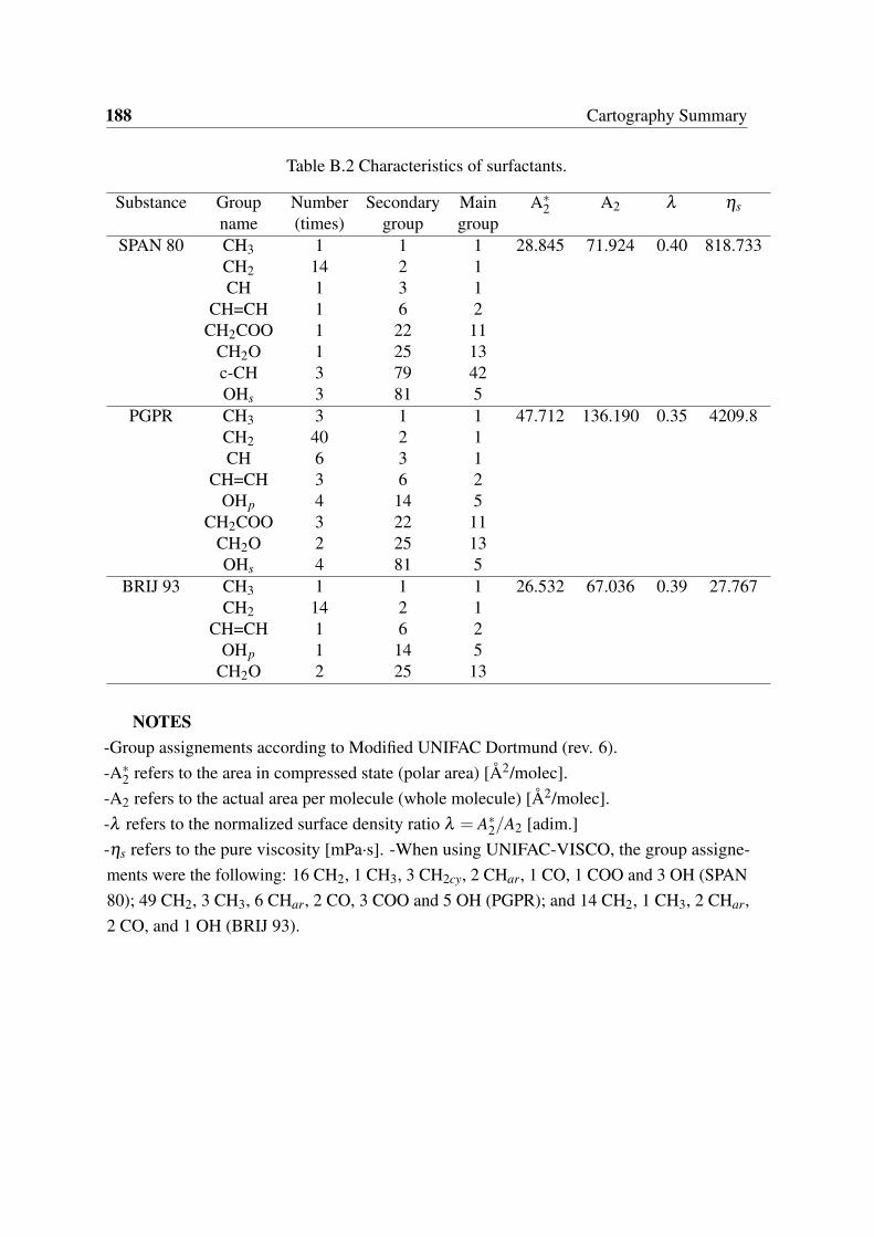
188 Cartography Summary
Table B.2 Characteristics of surfactants.
Substance Group Number Secondary Main A∗2 A2 λ ηs
name (times) group groupSPAN 80 CH3 1 1 1 28.845 71.924 0.40 818.733
CH2 14 2 1CH 1 3 1
CH=CH 1 6 2CH2COO 1 22 11
CH2O 1 25 13c-CH 3 79 42OHs 3 81 5
PGPR CH3 3 1 1 47.712 136.190 0.35 4209.8CH2 40 2 1CH 6 3 1
CH=CH 3 6 2OHp 4 14 5
CH2COO 3 22 11CH2O 2 25 13OHs 4 81 5
BRIJ 93 CH3 1 1 1 26.532 67.036 0.39 27.767CH2 14 2 1
CH=CH 1 6 2OHp 1 14 5
CH2O 2 25 13
NOTES-Group assignements according to Modified UNIFAC Dortmund (rev. 6).-A∗
2 refers to the area in compressed state (polar area) [Å2/molec].-A2 refers to the actual area per molecule (whole molecule) [Å2/molec].-λ refers to the normalized surface density ratio λ = A∗
2/A2 [adim.]-ηs refers to the pure viscosity [mPa·s]. -When using UNIFAC-VISCO, the group assigne-ments were the following: 16 CH2, 1 CH3, 3 CH2cy, 2 CHar, 1 CO, 1 COO and 3 OH (SPAN80); 49 CH2, 3 CH3, 6 CHar, 2 CO, 3 COO and 5 OH (PGPR); and 14 CH2, 1 CH3, 2 CHar,2 CO, and 1 OH (BRIJ 93).

Appendix C
Experimental annex
C.0.1 Preparation of experimental calibration curves
Verifications concerning the calibration standards were previously performed, in order tocheck if the values of of λmax were influenced or not by the substances present in theexperiments. All the oil substances (dodecane, hexadecane, isopropyl myristate and iso-propyl palmitate), active ingredient (mandelic acid), surfactants (SPAN 80 and BRIJ 93)and salt (NaCl) were purchased in Sigma Aldrich and used as received. Concerning thesurfactant PGPR, it was obtained from DANISCO. The water employed for all tests waspreviously deionized and mili-Q filtrated by a Millipore apparatus. On the one hand, different’stocksolutions’ were prepared according to the following procedure using SPAN 80 anddodecane. First, a volume of water was brought into contact with a volume of pure dodecaneoil in order to saturate with oil. The mixture was shaken vigorously using a magnetic stirrerduring 24h. After shaking, the two-phase dispersion was added to a separating funnel andallowed to separate both organic and aqueous layers during 24h. Following this, the aqueousphase was recovered and placed in a second separating funnel with surfactant SPAN 80in order to achieve saturation with surfactant. Again, a certain time for equilibration wasallowed (3 days) and the aqueous phase was taken. The absorption curves of the aqueousphases coming from the previous steps were measured by the UV-spectrometer using purewater as blank. In addition, a diluted solution of mandelic acid was also prepared by usingthe aqueous phase coming from the last step (after adding surfactant). Fig. C.1a showsthe typical spectras obtained when measuring these ’stocksolutions’. Fig. C.1b shows thetypical spectras obtained when only mandelic acid and water are present in the solution. Asone can see, the λmax for mandelic acid corresponds to a wavelength of 257 nm, however, itwas evinced that oil or surfactant, likely transferred to the aqueous solution from the organicphase, can also contribute to the absorbance signal. For example, after bringing into contact

190 Experimental annex
water, oil and surfactant, a λmax was shown around 273 nm. After mixing water with oil, theeffect was much less pronounced, no clear maximum peak was observed, but a magnificationeffect of 0.05 on the whole absorption curve was observed.
(a) (b)
Fig. C.1 a) Typical UV-spectra for liquid mixtures exmployed for calibration purposes in thiswork. b) UV-spectras when employing only mandelic acid and water.
These findings have important implications concerning the obtaining of a correct cali-bration curve, since that if there is an excessive magnification on the absorbance signal bycompounds distinct from the molecule of interest, the lecture of λmax could be seriouslymisleading. With the purpose of study and correcting these phenomena, series of calibra-tion curves were prepared using as solvent different stock solutions containing differentcombinations of substances solubilized; the first one containing only water; the second,water and salt; a third one water, salt and possible oil solubilized; and a last one containingwater, salt, oil and surfactant. The results of the calibration curves reading the absorbanceat a wavelength of 257 nm and considering pure water as blank are shown in Fig.C.2a. Asone can see, a baseline interference on the absorbance (0.4809 units) occured only whensurfactant was present in the solution and the considered blank was pure water. This effectwas independent of the concentration of the analyte, affecting the intercept of the calibrationcurve, but not its slope. All the other calibration lines agreed with a slope of approximately1.1 with a zero intercept. Fortunately, it was observed that in order to eliminate this effect,the stock solution employed as solvent for the preparation of the calibration standards canbe used as blank (Fig.C.2b). In this way, the rise of the signal produced by the concomitantsubstances (oil or surfactant present in the solution), can be corrected (See Fig. C.2a). As analternative (preferable in a practical way), it was also verified that dilutions higher than 1/15can generally decrease the baseline to zero (see Fig. C.2b). However, this would decrease

191
simultaneously the concentration of mandelic acid, therefore it would be only recommendedif the analyte concentration was greater enough to not result out of the detection limits of thetechnique.
(a) (b)
Fig. C.2 a) Calibration lines employing pure water as blank for UV lectures. b) Calibrationlines employing the respective stock solutions as blanks for UV lecture.
C.0.2 Preparation of samples for comparison of UNIFAC methods
The procedure for the preparation of the samples was the following. First, 6.5 mL aliquotesfrom a 0.5 M solution of mandelic acid were added to different labeled test tubes in order toobtain a final mass amount of 0.5 g of MA in each tube (with the exception of samples 19-24,where this mass amount was varied from 0.5 to 0.25). Subsequently, the solutions were madeup with deionized water until a total volume of approximately 8.5 mL (except samples 7-12,where volumes were allowed to vary from 7.5 to 10.5). Then, 0.5 g of pure dodecane oilwere weighted in every tube (besides those from 13-18, where the allowed variation wasfrom 0.5 to 3). As a last step, approximately 0.4 g of SPAN 80 surfactant was added by usinga syringe (with the exception of samples 1-6, where this amount was varied from 0.1 to 1.5).A Pasteur pippette was placed until the bottom of tubes with the intention of sampling theaqueous phase once the equlibrium was achieved. The upper part of the tube was completelysealed in order to avoid evaporation losses. It was observed that the time needed for thisequilibration, in the experimental conditions of this work (298 K), was about 1 day for mostof the samples used. After this time, each sample of aqueous phase obtained by the Pasteurpipettes was diluted 40 times with deionized water and the absorbance was measured at thewavelenght 257 nm by the UV-spectrometer. Table C.1 summarizes the characteristics ofsamples.

192 Experimental annex
Table C.1 Characteristics of samples in study for comparison of UNIFAC methods. Thesystem studied was: Mandelic acid + Water + SPAN 80 + Dodecane.
MA initialSample molarity φv moil/msur f . Kcd (pred.) Kcd (exp.) ε (error)
1 0.39 0.92 4.78 0.90 2.26 -60.082 0.37 0.91 2.22 1.21 1.78 -31.653 0.39 0.89 1.19 1.63 0.59 174.434 0.39 0.87 0.89 1.85 1.41 31.385 0.39 0.85 0.52 2.28 0.44 422.596 0.40 0.81 0.38 2.48 0.91 172.757 0.44 0.87 1.37 1.54 0.46 233.288 0.47 0.87 1.33 1.57 0.80 95.449 0.52 0.86 1.28 1.62 0.82 96.8510 0.39 0.88 0.97 1.78 0.36 398.6211 0.34 0.90 1.31 1.54 1.09 40.6312 0.31 0.91 1.32 1.52 1.72 -11.4913 0.39 0.67 7.21 0.79 0.18 348.7614 0.39 0.70 6.02 0.83 0.65 28.0815 0.39 0.74 4.99 0.88 1.13 -22.0716 0.39 0.78 3.80 0.97 0.73 31.3317 0.39 0.83 2.32 1.18 1.46 -18.9818 0.39 0.89 1.22 1.60 0.66 142.7319 0.39 0.88 1.31 1.55 1.59 -2.6920 0.35 0.88 1.44 1.47 0.51 186.0921 0.31 0.88 1.34 1.50 0.37 310.6222 0.27 0.89 1.26 1.53 0.63 142.6423 0.23 0.88 1.26 1.52 - -24 0.19 0.89 1.24 1.52 2.68 -43.4425 0.39 0.88 1.30 1.56 0.11 1358.1626 0.39 0.88 1.27 1.57 0.30 415.9027 0.38 0.88 1.35 1.53 1.39 10.1228 0.40 0.87 1.49 1.46 1.29 13.44
NOTES-The predicted distribution coefficients Kcd (pred.) shown in the table were obtained by usingModified UNIFAC Dortmund (Constantinescu, 2016). For the calculation of the experimentaldistribution coefficient Kcd (exp.), it was considered a total continuous phase volume (volumeof oil + volume of surfactant) same as the one at the moment of sample preparation.-Samples 25, 26, 27 and 28 were prepared with NaCl concentrations of 1, 2, 3 and 4%.-The relative error ε , was calculated according to the formula Kcd(pred.)−Kcd(exp.)
Kcd(exp.) x 100.-Empty values in table imply that mass balance for the continuous phase was negative.

193
C.0.3 Effect of salt content and blank/dilution media
The preparation of samples was carried out using a similar procedure to the one previouslyexplained (see C.0.2). However, different mandelic acid concentrations, NaCl content, aswell as oil/surfactant ratios were studied. Table C.2 summarizes the characteristics of allsamples. Representative examples of the typical third layers appearing in this test, are shownin Fig. C.3. The sample letter A refers to a 2% NaCl aqueous solution employed as dispersedphase. The letter B refers to a dispersed phase without salt. In addition, Fig. C.4 shows aglobal picture of all samples, before and after the equilibrium was achieved.
(a) (b) (c)
(d) (e) (f)
Fig. C.3 Samples at the end of equilibrium tests, φv ≈ 0.7 for all samples, oil/surfactantratios≈1, 7 and 15 for samples number 1, 2 and 3 respectively. Letter A means a 2% NaClcontent in the aqueous phase, letter B means that there is no salt.

194 Experimental annex
Table C.2 Characteristics of samples in study of effect of salt content and blank/dilutionmedia.
Water Stock Water StockMA inital Kcd Kcd Kcd ε ε
Sample molarity φv moil/msur f . (pred.) (exp.) (exp.) (error) (error)1A 8.55E-04 0.73 1.03 1.58 - - - -2A 8.60E-04 0.70 7.35 0.75 - - - -3A 8.61E-04 0.69 14.70 0.66 - - - -4A 8.56E-03 0.73 1.00 0.45 0.87 1.01 230.05 48.945A 8.62E-03 0.70 7.22 0.31 0.55 1.20 125.24 -41.686A 8.59E-03 0.70 14.61 0.47 1.40 1.68 31.17 -63.157A 8.75E-02 0.73 0.99 0.76 1.72 0.36 145.92 423.848A 8.75E-02 0.70 7.48 0.46 0.85 0.69 118.31 47.209A 8.69E-02 0.70 14.81 0.66 0.71 0.82 39.45 11.771B 8.51E-04 0.73 1.01 1.91 - - - -2B 8.57E-04 0.69 6.55 1.10 - - - -3B 8.55E-04 0.69 14.65 0.98 - - - -4B 8.59E-03 0.73 1.00 1.21 0.33 0.11 265.41 971.465B 8.52E-03 0.70 7.54 0.70 0.39 0.34 81.17 109.596B 8.58E-03 0.70 15.14 0.64 0.31 0.17 108.46 266.497B 8.59E-02 0.73 0.97 1.14 0.32 0.51 260.39 125.518B 8.55E-02 0.70 6.86 0.67 0.36 0.52 83.21 29.559B 8.57E-02 0.70 15.36 0.60 0.06 1.42 845.89 -57.85
NOTES-Two measurements were performed per sample to obtain two distribution coefficients, thefirst one employing as a blank and dilution media, pure water (Water), and the second,employing the respective stock solution (Stock).-The predicted distribution coefficients Kcd (pred.) shown in the table were obtained byusing Modified UNIFAC Dortmund (Constantinescu, 2016). For the calculation of theexperimental distribution coefficients Kcd (exp.), it was considered a total continuous phasevolume (volume of oil + volume of surfactant) same as the one at the moment of samplepreparation.-The relative error ε , was calculated according to the formula Kcd(pred.)−Kcd(exp.)
Kcd(exp.) x 100.-Empty values in table imply that mass balance for the continuous phase was negative.-The UV lecture of samples with salt and low and median concentrations of mandelic acid(from 1A to 6A), as well as samples without salt at low concentrations of mandelic acid(from 1B to 3B) were performed without dilution. A 1/15 dilution with the respective dilutionmedia was performed for the rest of samples.

195
(a)
(b)
(c)
(d)
Fig.
C.4
Sam
ples
for
dist
ribu
tion
coef
ficie
ntde
term
inat
ion.
The
sam
ple
lette
rA
refe
rsto
a2%
NaC
laqu
eous
solu
tion
empl
oyed
asdi
sper
sed
phas
e.T
hele
tterB
refe
rsto
asa
mpl
epr
epar
edw
ithou
tsal
t.T
heap
prox
imat
eoi
l/su
rfac
tant
ratio
empl
oyed
wer
eth
efo
llow
ing:
sam
ple
num
bers
1,4
and
7(r≈
1),2
,5an
d8
(r≈
7.5)
and
3,6
and
9(r≈
15).
Figu
res
a)an
db)
wer
eta
ken
right
afte
rsam
ple
prep
arat
ion.
Figu
res
c)an
dd)
afte
rthe
equi
libri
umw
asac
hiev
ed.
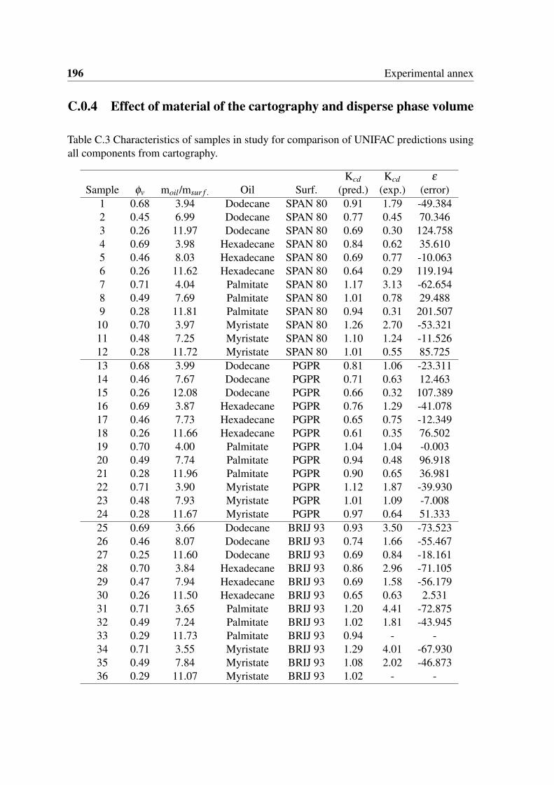
196 Experimental annex
C.0.4 Effect of material of the cartography and disperse phase volume
Table C.3 Characteristics of samples in study for comparison of UNIFAC predictions usingall components from cartography.
Kcd Kcd ε
Sample φv moil/msur f . Oil Surf. (pred.) (exp.) (error)1 0.68 3.94 Dodecane SPAN 80 0.91 1.79 -49.3842 0.45 6.99 Dodecane SPAN 80 0.77 0.45 70.3463 0.26 11.97 Dodecane SPAN 80 0.69 0.30 124.7584 0.69 3.98 Hexadecane SPAN 80 0.84 0.62 35.6105 0.46 8.03 Hexadecane SPAN 80 0.69 0.77 -10.0636 0.26 11.62 Hexadecane SPAN 80 0.64 0.29 119.1947 0.71 4.04 Palmitate SPAN 80 1.17 3.13 -62.6548 0.49 7.69 Palmitate SPAN 80 1.01 0.78 29.4889 0.28 11.81 Palmitate SPAN 80 0.94 0.31 201.507
10 0.70 3.97 Myristate SPAN 80 1.26 2.70 -53.32111 0.48 7.25 Myristate SPAN 80 1.10 1.24 -11.52612 0.28 11.72 Myristate SPAN 80 1.01 0.55 85.72513 0.68 3.99 Dodecane PGPR 0.81 1.06 -23.31114 0.46 7.67 Dodecane PGPR 0.71 0.63 12.46315 0.26 12.08 Dodecane PGPR 0.66 0.32 107.38916 0.69 3.87 Hexadecane PGPR 0.76 1.29 -41.07817 0.46 7.73 Hexadecane PGPR 0.65 0.75 -12.34918 0.26 11.66 Hexadecane PGPR 0.61 0.35 76.50219 0.70 4.00 Palmitate PGPR 1.04 1.04 -0.00320 0.49 7.74 Palmitate PGPR 0.94 0.48 96.91821 0.28 11.96 Palmitate PGPR 0.90 0.65 36.98122 0.71 3.90 Myristate PGPR 1.12 1.87 -39.93023 0.48 7.93 Myristate PGPR 1.01 1.09 -7.00824 0.28 11.67 Myristate PGPR 0.97 0.64 51.33325 0.69 3.66 Dodecane BRIJ 93 0.93 3.50 -73.52326 0.46 8.07 Dodecane BRIJ 93 0.74 1.66 -55.46727 0.25 11.60 Dodecane BRIJ 93 0.69 0.84 -18.16128 0.70 3.84 Hexadecane BRIJ 93 0.86 2.96 -71.10529 0.47 7.94 Hexadecane BRIJ 93 0.69 1.58 -56.17930 0.26 11.50 Hexadecane BRIJ 93 0.65 0.63 2.53131 0.71 3.65 Palmitate BRIJ 93 1.20 4.41 -72.87532 0.49 7.24 Palmitate BRIJ 93 1.02 1.81 -43.94533 0.29 11.73 Palmitate BRIJ 93 0.94 - -34 0.71 3.55 Myristate BRIJ 93 1.29 4.01 -67.93035 0.49 7.84 Myristate BRIJ 93 1.08 2.02 -46.87336 0.29 11.07 Myristate BRIJ 93 1.02 - -

197
C.0.5 Predicted and experimental release experiments
Table C.4 Characterization of SPAN 80 emulsions for release experiments.
No. Oil φm ro/s Ddroplet G’be f ore G’a f ter D (pred) D (exp) ε
1 D 0.91 1.07 12.39 1276 1489 1.28E-10 1.27E-10 1.232 D 0.91 2.58 12.96 410 500 1.66E-10 1.66E-10 -0.193 D 0.91 5.13 13.90 196 229 1.63E-10 1.70E-10 -4.334 D 0.93 1.02 12.93 2059 2110 1.01E-10 9.49E-11 5.995 D 0.93 2.37 13.91 800 976 1.24E-10 1.26E-10 -1.256 D 0.93 4.84 15.26 350 382 1.28E-10 1.33E-10 -4.117 D 0.95 1.00 13.49 3528 3690 7.18E-11 6.47E-11 10.978 D 0.95 2.71 15.06 1315 1673 8.83E-11 7.19E-11 22.879 D 0.95 5.39 17.45 674 849 8.30E-11 9.08E-11 -8.5810 H 0.91 1.03 9.22 1845 2174 6.88E-11 6.09E-11 13.0811 H 0.91 2.50 9.69 916 1033 1.13E-10 9.65E-11 17.1312 H 0.91 5.17 10.46 458 573 1.30E-10 1.23E-10 4.9713 H 0.93 1.01 9.57 2736 2917 5.38E-11 4.60E-11 17.0114 H 0.93 2.28 10.98 1925 1719 8.31E-11 7.07E-11 17.5615 H 0.93 4.63 12.92 955 1171 1.01E-10 7.83E-11 29.5016 H 0.95 1.02 9.96 5463 5218 3.82E-11 2.97E-11 28.7717 H 0.95 2.47 12.38 2780 2225 6.20E-11 5.49E-11 12.9118 H 0.95 5.04 16.61 1797 1776 7.00E-11 6.85E-11 2.0619 M 0.90 0.99 12.32 3568 4122 6.74E-11 9.18E-11 -26.5820 M 0.90 2.53 11.85 1882 2483 1.27E-10 1.64E-10 -22.7121 M 0.90 4.60 11.20 1226 1486 1.52E-10 2.52E-10 -39.7322 M 0.93 1.03 12.12 5219 6710 5.57E-11 8.91E-11 -37.5223 M 0.93 2.34 12.06 2546 2965 9.24E-11 1.51E-10 -38.8824 M 0.93 5.13 11.92 833 1049 1.18E-10 1.58E-10 -25.6025 P 0.90 1.01 9.57 3558 4212 4.25E-11 5.75E-11 -26.1526 P 0.90 2.47 9.84 2082 3064 7.63E-11 1.29E-10 -40.9127 P 0.91 5.18 10.26 1244 1508 9.21E-11 1.08E-10 -14.8528 P 0.93 0.98 9.95 4583 6036 3.25E-11 9.79E-11 -66.7829 P 0.93 2.43 9.95 3781 4014 5.90E-11 6.67E-11 -11.4830 P 0.93 4.84 9.94 1135 1228 7.21E-11 9.30E-11 -22.42
NOTES-D=dodecane; H=hexadecane; M=myristate; P=palmitate; S=SPAN 80.φm=dispersed phase mass fraction [adim.]; ro/s=oil/surfactant ratio moil/msur f . [adim.];Ddroplet=droplet diameter [µm]; G’=storage moduli before or after experiment [Pa]; D=fitteddiffusion coefficients for predicted (pred.) or experimental (exp.) curves [m2/s]; andε=relative error between D (pred.) and D (exp.).

198 Experimental annex
(a) No.1 (b) No.2 (c) No.3
(d) No.4 (e) No.5 (f) No.6
(g) No.7 (h) No.8 (i) No.9
(j) No.10 (k) No.11 (l) No.12
(m) No.13 (n) No.14 (o) No.15
Fig. C.5 Predicted and experimental release curves of SPAN 80 systems. Part (1/2).
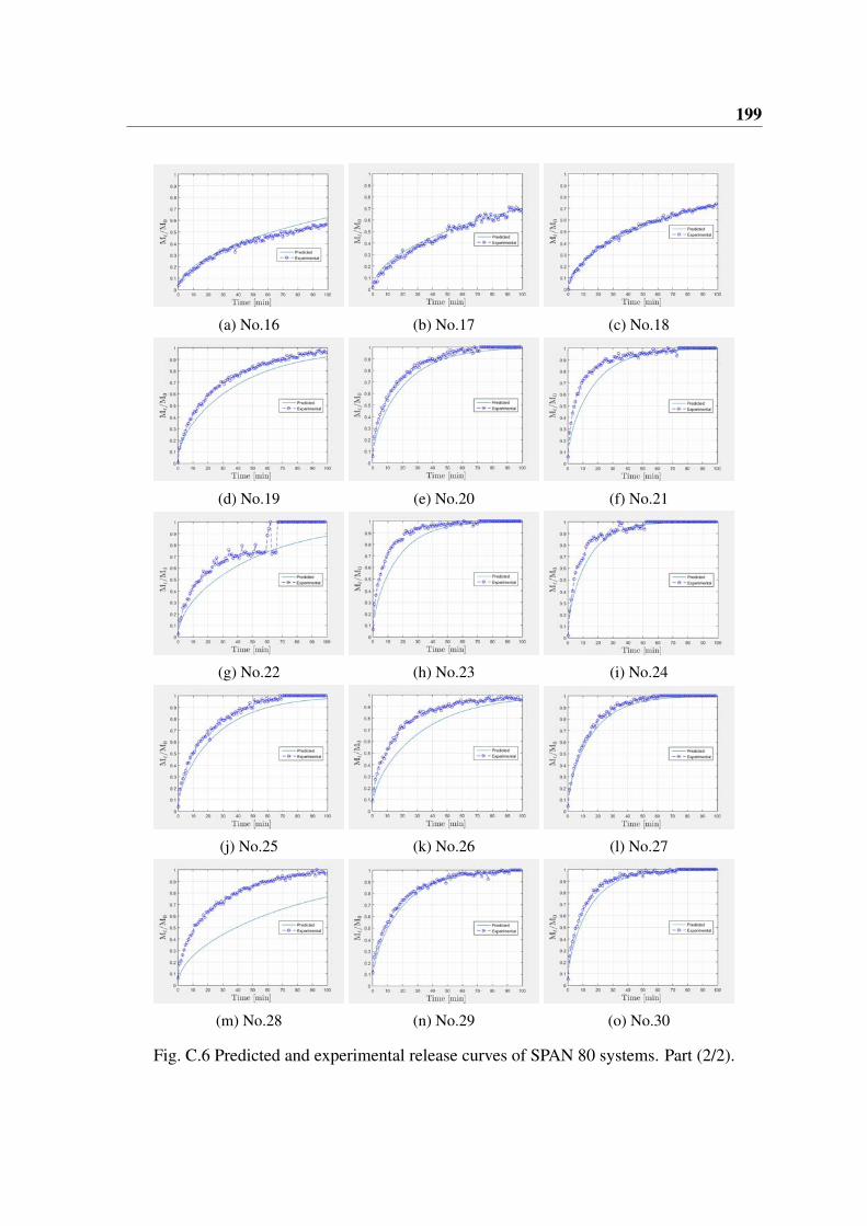
199
(a) No.16 (b) No.17 (c) No.18
(d) No.19 (e) No.20 (f) No.21
(g) No.22 (h) No.23 (i) No.24
(j) No.25 (k) No.26 (l) No.27
(m) No.28 (n) No.29 (o) No.30
Fig. C.6 Predicted and experimental release curves of SPAN 80 systems. Part (2/2).

200 Experimental annex
Table C.5 Characterization of PGPR emulsions for release experiments.
No. Oil φm ro/s Ddroplet G’be f ore G’a f ter D (pred.) D (exp.) ε
31 D 0.89 1.00 9.60 3730 5170 2.92E-10 2.05E-10 42.8332 D 0.90 2.53 9.79 1106 1246 2.53E-10 2.63E-10 -3.6433 D 0.90 4.89 10.47 289 337 2.05E-10 2.27E-10 -9.8834 D 0.92 1.00 9.76 3259 4020 2.20E-10 1.96E-10 12.3435 D 0.92 2.36 11.28 2189 2631 1.93E-10 2.28E-10 -15.3436 D 0.92 5.09 14.13 644 771 1.57E-10 1.72E-10 -8.7237 D 0.95 1.18 10.22 5565 6943 1.63E-10 1.33E-10 22.0538 D 0.95 2.90 13.44 2527 2438 1.32E-10 1.13E-10 16.3339 D 0.95 5.32 18.32 1281 1504 1.06E-10 1.45E-10 -26.8140 H 0.90 1.00 9.30 3766 4272 2.02E-10 1.70E-10 18.7941 H 0.90 2.57 9.30 2566 3110 2.09E-10 1.55E-10 34.8642 H 0.90 4.71 8.99 1060 1227 1.90E-10 2.11E-10 -9.8443 H 0.92 1.04 10.53 5221 6483 1.54E-10 1.09E-10 41.4444 H 0.92 2.55 11.00 5166 3023 1.61E-10 1.08E-10 49.0845 H 0.92 4.92 11.81 1525 1989 1.42E-10 1.08E-10 31.5246 H 0.95 0.99 11.56 1591 1191 1.07E-10 1.49E-10 -28.2947 H 0.95 2.68 12.87 3609 3804 1.07E-10 1.44E-10 -25.6648 H 0.95 4.69 14.37 2334 2788 9.54E-11 1.10E-10 -13.0249 M 0.90 1.01 9.37 4432 5352 1.46E-10 1.84E-10 -20.5850 M 0.88 2.60 8.86 3305 4000 2.31E-10 3.13E-10 -26.1551 M 0.87 4.84 8.08 1483 1486 2.37E-10 2.80E-10 -15.2552 M 0.91 1.02 9.39 6033 7379 1.44E-10 2.46E-10 -41.4453 M 0.92 2.35 10.33 3725 4110 1.55E-10 2.09E-10 -25.9254 M 0.92 5.13 11.86 2615 2244 1.52E-10 2.18E-10 -29.9355 P 0.90 0.99 9.59 4199 4391 9.22E-11 1.35E-10 -31.5956 P 0.90 2.60 10.12 3650 3903 1.22E-10 6.79E-11 79.4257 P 0.90 4.75 10.68 2734 3174 1.21E-10 2.62E-10 -53.6558 P 0.93 1.00 11.47 3354 3185 7.10E-11 1.32E-10 -46.0159 P 0.93 2.55 11.63 6204 4477 9.38E-11 3.29E-10 -71.4760 P 0.93 5.15 12.02 2722 2578 8.99E-11 2.12E-10 -57.56
NOTES-D=dodecane; H=hexadecane; M=myristate; P=palmitate; S=SPAN 80.φm=dispersed phase mass fraction [adim.]; ro/s=oil/surfactant ratio moil/msur f . [adim.];Ddroplet=droplet diameter [µm]; G’=storage moduli before or after experiment [Pa]; D=fitteddiffusion coefficients for predicted (pred.) or experimental (exp.) curves [m2/s]; andε=relative error between D (pred.) and D (exp.).

201
(a) No.31 (b) No.32 (c) No.33
(d) No.34 (e) No.35 (f) No.36
(g) No.37 (h) No.38 (i) No.39
(j) No.40 (k) No.41 (l) No.42
(m) No.43 (n) No.44 (o) No.45
Fig. C.7 Predicted and experimental release curves of PGPR systems. Part (1/2).

202 Experimental annex
(a) No.46 (b) No.47 (c) No.48
(d) No.49 (e) No.50 (f) No.51
(g) No.52 (h) No.53 (i) No.54
(j) No.55 (k) No.56 (l) No.57
(m) No.58 (n) No.59 (o) No.60
Fig. C.8 Predicted and experimental release curves of PGPR systems. Part (2/2).
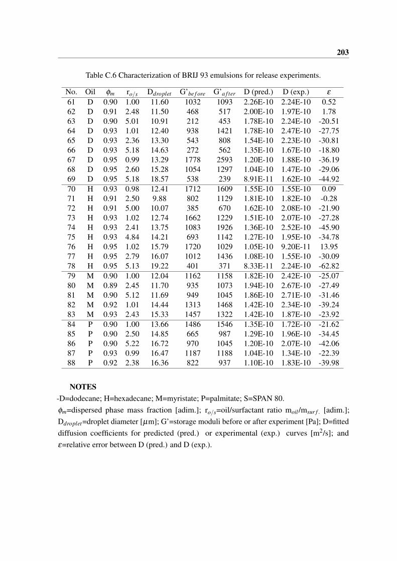
203
Table C.6 Characterization of BRIJ 93 emulsions for release experiments.
No. Oil φm ro/s Ddroplet G’be f ore G’a f ter D (pred.) D (exp.) ε
61 D 0.90 1.00 11.60 1032 1093 2.26E-10 2.24E-10 0.5262 D 0.91 2.48 11.50 468 517 2.00E-10 1.97E-10 1.7863 D 0.90 5.01 10.91 212 453 1.78E-10 2.24E-10 -20.5164 D 0.93 1.01 12.40 938 1421 1.78E-10 2.47E-10 -27.7565 D 0.93 2.36 13.30 543 808 1.54E-10 2.23E-10 -30.8166 D 0.93 5.18 14.63 272 562 1.35E-10 1.67E-10 -18.8067 D 0.95 0.99 13.29 1778 2593 1.20E-10 1.88E-10 -36.1968 D 0.95 2.60 15.28 1054 1297 1.04E-10 1.47E-10 -29.0669 D 0.95 5.18 18.57 538 239 8.91E-11 1.62E-10 -44.9270 H 0.93 0.98 12.41 1712 1609 1.55E-10 1.55E-10 0.0971 H 0.91 2.50 9.88 802 1129 1.81E-10 1.82E-10 -0.2872 H 0.91 5.00 10.07 385 670 1.62E-10 2.08E-10 -21.9073 H 0.93 1.02 12.74 1662 1229 1.51E-10 2.07E-10 -27.2874 H 0.93 2.41 13.75 1083 1926 1.36E-10 2.52E-10 -45.9075 H 0.93 4.84 14.21 693 1142 1.27E-10 1.95E-10 -34.7876 H 0.95 1.02 15.79 1720 1029 1.05E-10 9.20E-11 13.9577 H 0.95 2.79 16.07 1012 1436 1.08E-10 1.55E-10 -30.0978 H 0.95 5.13 19.22 401 371 8.33E-11 2.24E-10 -62.8279 M 0.90 1.00 12.04 1162 1158 1.82E-10 2.42E-10 -25.0780 M 0.89 2.45 11.70 935 1073 1.94E-10 2.67E-10 -27.4981 M 0.90 5.12 11.69 949 1045 1.86E-10 2.71E-10 -31.4682 M 0.92 1.01 14.44 1313 1468 1.42E-10 2.34E-10 -39.2483 M 0.93 2.43 15.33 1457 1322 1.42E-10 1.87E-10 -23.9284 P 0.90 1.00 13.66 1486 1546 1.35E-10 1.72E-10 -21.6285 P 0.90 2.50 14.85 665 987 1.29E-10 1.96E-10 -34.4586 P 0.90 5.22 16.72 970 1045 1.20E-10 2.07E-10 -42.0687 P 0.93 0.99 16.47 1187 1188 1.04E-10 1.34E-10 -22.3988 P 0.92 2.38 16.36 822 937 1.10E-10 1.83E-10 -39.98
NOTES-D=dodecane; H=hexadecane; M=myristate; P=palmitate; S=SPAN 80.φm=dispersed phase mass fraction [adim.]; ro/s=oil/surfactant ratio moil/msur f . [adim.];Ddroplet=droplet diameter [µm]; G’=storage moduli before or after experiment [Pa]; D=fitteddiffusion coefficients for predicted (pred.) or experimental (exp.) curves [m2/s]; andε=relative error between D (pred.) and D (exp.).

204 Experimental annex
(a) No.61 (b) No.62 (c) No.63
(d) No.64 (e) No.65 (f) No.66
(g) No.67 (h) No.68 (i) No.69
(j) No.70 (k) No.71 (l) No.72
(m) No.73 (n) No.74 (o) No.75
Fig. C.9 Predicted and experimental release curves of BRIJ 93 systems. Part (1/2).
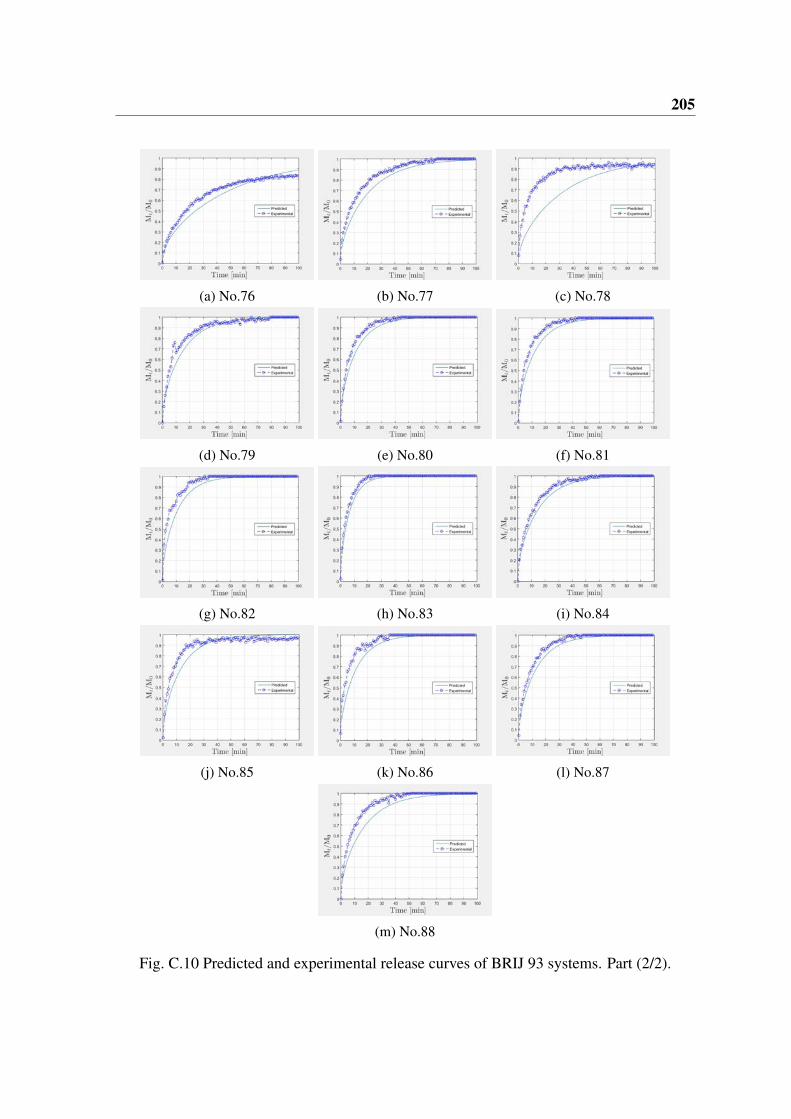
205
(a) No.76 (b) No.77 (c) No.78
(d) No.79 (e) No.80 (f) No.81
(g) No.82 (h) No.83 (i) No.84
(j) No.85 (k) No.86 (l) No.87
(m) No.88
Fig. C.10 Predicted and experimental release curves of BRIJ 93 systems. Part (2/2).
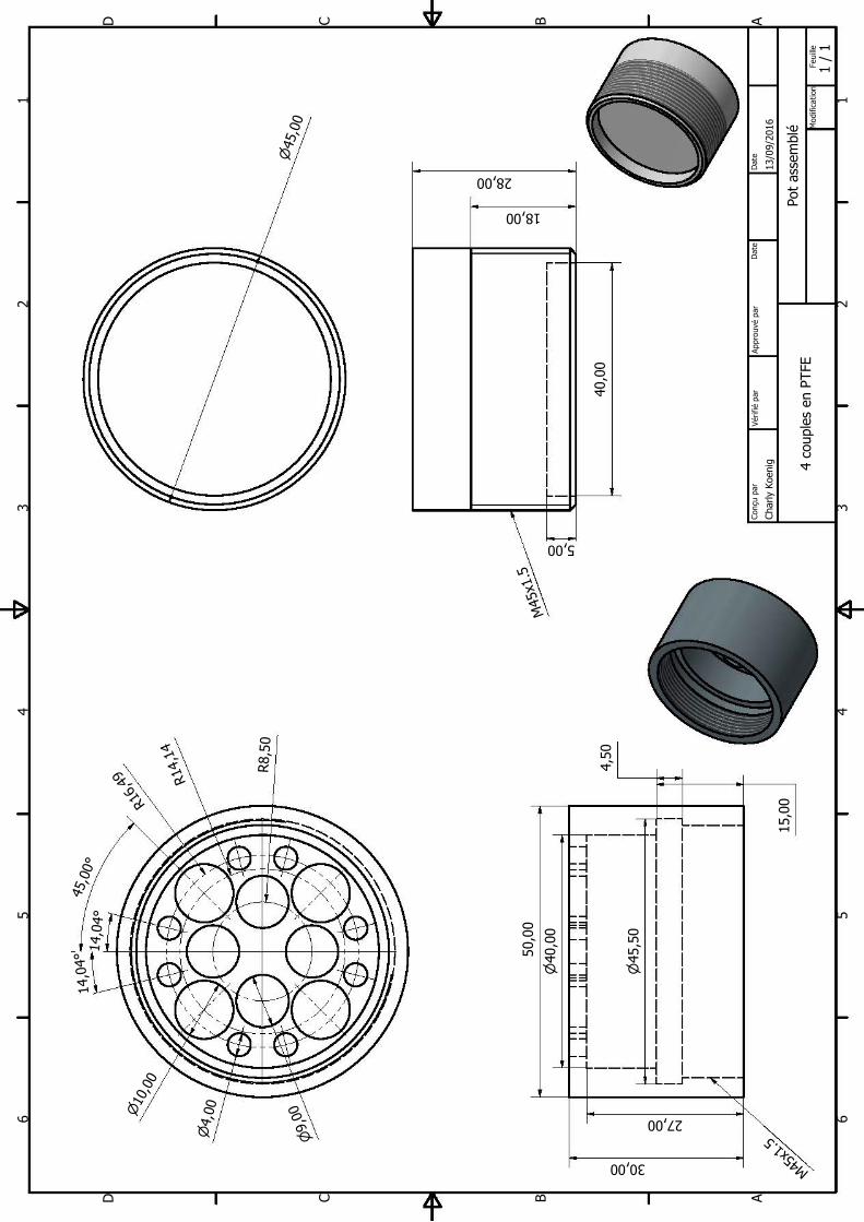
1 1
2 2
3 3
4 4
5 5
6 6
AA
BB
CC
DD
Pot
asse
mbl
é
4
coup
les
en P
TFE
Char
ly K
oeni
g13
/09/
2016
Conç
u pa
rVé
rifié
par
Appr
ouvé
par
Dat
e
1 /
1 M
odifi
catio
nFe
uille
Dat
e
30,00 M45x1
.5
50,0
0
10,
00
9,
00
4,
00
45
,00
40,0
0
5,00
18,00
M45
x1.5
28,00
4,50
15,0
0
45
,50
40
,00
27,00
R8,5
0
R14,
14
R16,
49
45,0
0°14
,04°
14,0
4°
1 ....
r ~ 1
1
1
1
1
1
1
1
1
1
1
1
1
! r 1.
~

207
Transfert de matière dans les milieux complexes.Ingénierie inverse: de la propriété d’usage au matériau
Mots clés: Ingénierie inverse, emulsion hautement concentrée, diffusion, rhéologie.
Au cours de la dernière décennie, l’utilisation croissante de nombreuses nouvelles technologiescomme des systèmes de livraison contrôlée a incité un développement empirique coûteux de systèmesnouveaux et efficaces. Pour faciliter une conception plus raisonnable et une optimisation, faisantface à l’ensemble de possibilités existantes, n’importe quelle solution qui pourrait semiautomatiserle développement de produits apporteraient l’aide précieuse aux utilisateurs (des scientifiques deformulation et des éducateurs). Ceci faciliterait l’importance essentielle de choisir les matériels justespour l’application correcte. Dans cette thèse, un projet à long terme concernant une génie inverseest proposé, commençant d’une propriété d’utilisation finale (libération contrôlée), la cible mondialeest de développer une méthodologie de conception de produit qui nous permet de déterminer lescaractéristiques optimales d’une formulation à préparer: les phases, la composition, le type d’interface,la taille et la distribution d’objets actuels, l’équilibre de phase, la diffusion dans des phases et lecaractère évolutionnaire du matériel. Dans la considération d’un exemple de commodité de systèmestructuré et dispersé: des émulsions fortement concentrées, le problème de design a été décomposédans un ordre hierachical de sous-problèmes ou des boîtes, combinant les modèles constitutifs quiévaluent le transport de masse de principe actif comme une fonction de paramètres de formulation etdes techniques assistées par ordinateur comme la modélisation moléculaire pour le volume/surfacede molécules, ou des modèles d’UNIFAC pour des prédictions d’équilibre aussi bien que pour desévaluations de viscosités de mélange. Un ultérieur design de factoriel d’expériences virtuelles apermis d’obtenir une description quantitative de la sortie selon les paramètres modèles et une analysecomposante principale a évalué l’importance des variables. En utilisant une cartographie basée surtrois tensio-actifs (pour SPAN 80, PGPR et BRIJ 93), quatre huiles (dodecane, hexadecane, isopropylmyristate et isopropyl palmitate) et l’acide mandelic comme le principe actif, le modèle ab initiophysicochimique a été expérimentalement validé. Les résultats montrent que le modèle mécanistesystématiquement prévoit la diffusion du principe actif d’émulsions à un moyen récepteur dans desparfaites ’sink’ conditions. Cette approche de génie inverse a montré pour être d’intérêt très élevé dansle domaine de formulation en permettant des études préliminaires examinantes rapides et robustes surune large gamme de composants aussi bien que des outils de prédiction précis et rigoureux optimiserla sortie contrôlée d’un système identifié. On cela recommande entièrement de mettre en œuvre sesextensions à d’autre semblable systèmes.

208 Experimental annex
Mass transfer within complex media.Reverse Engineering: From usage property to materialKeywords: Reverse engineering, highly concentrated emulsion, diffusion, rheology
In the past decade, the growing use of numerous novel technologies as controlled-delivery systemshas prompted a costly trial-and-error development of new and effective systems. In order to facilitatea more rational design and optimization, facing the set of existing possibilities, any solution thatcould semiautomate the product development would bring precious help to the users (formulationscientists and educators). This would facilitate the essential importance of choosing the right materialsfor the correct application. In this thesis, a long-term project concerning a reverse engineering isproposed, starting from a final usage property (controlled release), the global target is to developa product design methodology which allows us to determine the optimal features of a formulationto prepare: phases in presence, composition, interface type, size and distribution of current objects,phase equilibrium, diffusion within phases and evolutionary character of the material. Consideringa convenience example of structured-dispersed system: highly concentrated emulsions, the designproblem has been decomposed into a hierarchical sequence of subproblems or boxes, combiningconstitutive models that estimate the active ingredient mass transport as a function of formulationparameters and computer-aided techniques such as molecular modeling for volume/area of molecules,or UNIFAC models for equilibria predictions as well as for mixture viscosities estimations. Asubsequent full factorial design of virtual experiments has allowed to obtain a quantitative descriptionof the release depending on the model parameters, and a principal component analysis has assessedthe importance of the variables. Using a cartography focused on three surfactants (SPAN 80, PGPRand BRIJ 93), four oils (dodecane, hexadecane, isopropyl myristate and isopropyl palmitate) andmandelic acid as an active ingredient, the ab-initio physicochemical model has been experimentallyvalidated. Results show that the mechanistic model consistently predicts the diffusion of the activeingredient from emulsions to a release medium in perfect sink conditions. This reverse engineeringapproach is showing to be of very high interest in the domain of formulation by allowing fast androbust screening preliminary studies on a broad range of components as well as precise and rigorousprediction tools to optimize controlled release from an identified system. It is fully recommended toimplement its extensions to other similar disperse systems.
Copyright © 2022 FDOKUMEN