This content has been downloaded from IOPscience. Please scroll down to see the full text.

Download details:

IP Address: 27.24.158.131

This content was downloaded on 15/10/2013 at 23:26

Please note that terms and conditions apply.

Deterministic point inclusion methods for computational applications with complex geometry

View the table of contents for this issue, or go to the journal homepage for more

2008 Comput. Sci. Disc. 1 015004

(http://iopscience.iop.org/1749-4699/1/1/015004)

Home Search Collections Journals About Contact us My IOPscience

Deterministic point inclusion methods forcomputational applications with complex geometry

Ahmed Khamayseh1 and Andrew Kuprat2

1 Computer Science and Mathematics Division, MS 6367, Oak Ridge National Laboratory,Oak Ridge, TN 37831, USA2 Biological Sciences Division, Pacific Northwest National Laboratory, MSIN P7-58,Richland, WA 99352, USAE-mail: khamaysehak@ornl.gov and andrew.kuprat@pnl.gov

Received 14 August 2007, in final form 26 February 2008Published 20 November 2008Computational Science & Discovery 1 (2008) 015004 (22pp)doi:10.1088/1749-4699/1/1/015004

Abstract. A fundamental problem in computation is finding practical and efficientalgorithms for determining if a query point is contained within a model of a three-dimensionalsolid. The solid is modeled using a general boundary representation that can contain polygonalelements and/or parametric patches. We have developed two such algorithms: the first is basedon a global closest feature query, and the second is based on a local intersection query. Bothalgorithms work for two- and three-dimensional objects. This paper presents both algorithms,as well as the spatial data structures and queries required for efficient implementation ofthe algorithms. Applications for these algorithms include computational geometry, meshgeneration, particle simulation, multiphysics coupling, and computer graphics. These methodsare deterministic in that they do not involve random perturbations of diagnostic rays castfrom the query point in order to avoid ‘unclean’ or ‘singular’ intersections of the rays withthe geometry. Avoiding the necessity of such random perturbations will become increasinglyimportant as geometries become more convoluted and complex.

Computational Science & Discovery 1 (2008) 015004 www.iop.org/journals/csd© 2008 IOP Publishing Ltd 1749-4699/08/015004+22$30.00

Computational Science & Discovery 1 (2008) 015004 A Khamayseh and A Kuprat

Contents

1. Introduction 21.1. Preliminary information . . . . . . . . . . . . . . . . . . . . . . . . . . . . . . . . . . . . . . 3

2. Global point inclusion method 42.1. Synthetic normal method . . . . . . . . . . . . . . . . . . . . . . . . . . . . . . . . . . . . . 4

3. Directed point inclusion method 6

4. Geometric partitioning using an skd-tree 104.1. skd-tree construction . . . . . . . . . . . . . . . . . . . . . . . . . . . . . . . . . . . . . . . 114.2. Nearest boundary point query . . . . . . . . . . . . . . . . . . . . . . . . . . . . . . . . . . . 134.3. Line segment intersection query . . . . . . . . . . . . . . . . . . . . . . . . . . . . . . . . . 144.4. Bounding box intersection query . . . . . . . . . . . . . . . . . . . . . . . . . . . . . . . . . 15

5. Applications 155.1. Hybrid mesh generation and adaptivity . . . . . . . . . . . . . . . . . . . . . . . . . . . . . . 165.2. Field transfer in coupled multiphysics . . . . . . . . . . . . . . . . . . . . . . . . . . . . . . 18

6. Discussion 20

Acknowledgments 22

References 22

1. Introduction

A problem of practical importance for three-dimensional computational applications is determining if a querypoint is contained within a model of a solid physical object. In our applications, this query is executed animmense number of times on complex models with high accuracy demands.

The efficiency of this query depends largely on the way the solid is modeled. For example, if the solidis modeled using constructive solid geometry (CSG), as the Boolean combination of implicit surfaces, pointcontainment queries can be performed extremely efficiently. However, modeling detailed objects in this fashioncan be impractical, and this representation is not well supported by contemporary computer-aided design(CAD) tools.

Commonly, solids are modeled using a general boundary representation (b-rep) [8], which representsthe boundary of the solid with a set of surface patches. The details of this representation can be found insection 1.1, but it supports mixtures of polyhedral and smooth (e.g. trimmed parametric) models. This choiceof representation is compatible with the output of many CAD tools and other common formats.

These algorithms were designed for use in engineering applications that contain complex geometricmodels. These applications make immense numbers of point inclusion queries against a single model, so weare interested in minimizing the repeated query time. This would normally indicate an extensive preprocessingstep, but the model complexity places restrictions on the space and time requirements of any preprocessingstep that we use.

In two dimensions, the point inclusion (sometimes referred to as point location) problem has been studiedextensively as the ‘point-in-polygon’ problem [7, 16, 17]. There are two predominant approaches to thisproblem: parity tests and winding numbers. The parity test approach involves shooting a ray from the querypoint, and counting the number of intersections that the ray makes with the polygon boundary. If the numberof intersections is odd, the point is inside the polygon. If the ray intersects a vertex, care must be taken toincrement the intersection count correctly. The winding number approach determines the number of revolutionsmade by the boundary around the query point. Unfortunately, this algorithm is difficult to implement correctly,and tends to be computationally expensive. A technique for curvilinear polygons (as well as a good survey ofthe problem) is presented by Hui [10].

A more general planar problem is that of point inclusion within a planar subdivision, where each cell is asimple polygon. Rather than perform n point-in-polygon tests, it is better to treat the subdivision as a whole.Methods that take this approach include slabbing and trapezoidal maps [4]. The basic idea of these approaches

2

Computational Science & Discovery 1 (2008) 015004 A Khamayseh and A Kuprat

is to preprocess the planar subdivision into a set of simple geometric regions, ordered along an axis. Theordering is used to determine which region a query point is in, and the simplicity of the region allows for anefficient containment test.

As is still fairly common in computational geometry, algorithms for higher dimensional point inclusionproblems are still scarce. The parity test and winding number approaches to point-in-polygon queries haveanalogues in three dimensions, although the problems found in the planar case are exacerbated in this setting.The parity test is predominant and relies upon the condition that a ray cast from the query point does notintersect a vertex or an edge. If a ray does hit one of these entities, a new ray can be cast in a random directionfrom the query point in an attempt to find a ‘clean’ intersection with the interior of a patch.

If the boundary is a convex polyhedra, several approaches are available. The Dobkin–Kirkpatrickhierarchy [5] is a theoretically elegant approach, but is not efficient in practice. The same comments applyto the method of Chazelle and Dobkin [3]. Another technique involves projecting the surface and the querypoint onto two parallel planes. After the projection, two-dimensional point inclusion algorithms are usedto identify the facets to test the query point against [16]. Unfortunately, realistic models are rarely convex,and convex decomposition of polyhedra is a difficult process [1], so these methods are not practical for ourapplication.

A complex method for point inclusion in a convex spatial cell-complex was developed by Preparataand Tamassia [18]. This method combines a persistent data structure and a dynamic planar point inclusionalgorithm to create a sweep-plane algorithm, which effectively performs the containment test in twodimensions.

The approach taken in this paper, like the parity test, involves shooting a ray from the query point.However, in contrast to the parity test, only the first intersection of the ray with the geometry is of importance,and the singular case where the ray intersects a vertex or an edge is allowed—the ray need never be randomlyperturbed in this case. The approach assumes the existence of a normal at any point on the surface. For‘degenerate’ cases where there is not a unique normal, such as an edge or vertex of a polyhedron, some simplecalculations are performed to determine an appropriate normal. The efficiency of this approach depends ontwo items: the efficiency of the normal finding operation (henceforth, assumed to be O(1)) and the efficiencyof nearest neighbor searches between the query point and the b-rep model. In the method of section 2, the rayis shot from the query point to the closest point on the geometry. A ‘synthetic normal’ is constructed usingincident patch normals at the closest point and a point inclusion test involving this normal is devised andrigorously proved. We note that in [2] this method is presented and a proof of correctness given for the caseof triangulated meshes. This method has, in fact, been used in several meshing codes at Los Alamos NationalLaboratory since the mid-1990s [12].

In the method of section 3, we remove the requirement that the ray be shot to the closest point on thegeometry, greatly reducing search time. Techniques for minimizing the search costs in these two methods aredescribed in section 4.

1.1. Preliminary information

Formally, the solid is represented by the compact set S ⊂ R3, such that the affine hull of S isR3. The boundary∂S of S is assumed to be an orientable 2-manifold. The boundary ∂S =

⋃ni=1 Pi , is composed of one or more

surface patches, Pi . For the sake of simplicity, surface patches are assumed to be at least C1 continuous ontheir interiors: each point interior to a surface patch has a unique normal (e.g. simple planar polygons andparametric patches). This continuity restriction can be lifted by recursive application of the techniques of thispaper, but this case will not be addressed further. The restriction that the boundary ∂S is 2-manifold impliesthat the neighborhood of every point p ∈ ∂S is homeomorphic to a 2-disc. Geometrically, this means thatthe surface does not self-intersect, and that there are no gaps in the boundary. The points where two or moreboundary curves meet will be called vertices, and the region of a boundary curve between two vertices will becalled an edge.

For each patch Pi , we assume the existence of a function Ni : Pi 7→ S2 that returns the unit outwardfacing normal for a query point in Pi , where S2 is the unit sphere. For points on ∂ Pi , Ni returns a vector whichis the limit of normals for interior points approaching the boundary point; this limit exists due to the presumed

3

Computational Science & Discovery 1 (2008) 015004 A Khamayseh and A Kuprat

continuity of the surface. Along the boundaries, we also assume the existence of function Ti : ∂ Pi 7→ S2

that returns the unit tangent vector of the boundary curve at p. (However, we do not assume that Ti exists atboundary vertices.) We assume Ti is oriented so that Ni × Ti is a unit vector pointing into the patch Pi .

Given ∂S and Ni , we determine the location of the query point q ∈ R3 with respect to S by evaluatingthe normal at a surface point p ‘near’ q. By comparing the ray q − p with Ni (p), we can readily determine ifq is contained in ∂S. The following sections contain two algorithms for this query that differ primarily in theirdefinition of ‘near’. The first algorithm is based on a global nearest surface point and the second is based onthe nearest surface point along a given ray.

2. Global point inclusion method

Conceptually, this algorithm expands a sphere, centered at the query point q, until the sphere reaches theboundary of the solid S. Because the solid is a compact set, the entire ball bounded by the sphere has the samelocation (inside or outside) as the query point. Let p ∈ ∂S be a point where the sphere first meets the boundary(i.e. the point on ∂S closest to the query point). Comparing the surface normal at p to the vector r = q − pwill allow us to determine if the sphere approached the surface from inside or from outside. We will take theconvention that points on the boundary are considered to be outside the solid.

Methods for calculating the point closest to q will be given in section 4. We then compute an outward-pointing surface normal np at p. If p is in the interior of patch Pi , then np is simply Ni (p). However, if p ison an edge or vertex of ∂S, there are a set of normals {Ni (p)} defined by the patches sharing p. Methods forcalculating a normal in this case are given in the follow subsections, which also contain proofs that ray-normalcomparison will yield the correct result. Algorithm 2.1 describes the top-level method.

Algorithm 2.1. Global point inclusion test

Input: Boundary ∂SQuery point q

Find a point p ∈ ∂S closest to qr← q− pIf ‖r‖ = 0 then

return outsideCalculate a normal np at pIf r · np > 0 then

return outsideelse

return insideOutput: inside or outside

2.1. Synthetic normal method

Our first approach to computing a normal for a point p on an edge or a vertex involves calculating a weightedaverage of the normals in the neighborhood of p. We call the result of this calculation a synthetic normal. LetB(p, ε) be an ε-radius solid ball centered at p. Define the ε-neighborhood of p as N (p, ε) = B(p, ε) ∩ ∂S.

We define the synthetic normal np at p to be

np ≡ limε→0

∫N (p,ε)

n dS

‖∫N (p,ε)

n dS‖, (2.1)

where n is the outward normal on the surface N (p, ε). If N (p, ε) is C1 continuous, as it is if p is in theinterior of a patch i , this definition gives the classical normal Ni (p). Otherwise, we produce a synthetic normal:the weighted average of the normals {Ni (p)} at p. Due to the limit taken in (2.1), the neighborhood of p iseffectively the union of a finite number of planar polygonal regions. For example, if p is on an edge, theadjacent patches are represented by half-planes with normals Ni (p).

4

Computational Science & Discovery 1 (2008) 015004 A Khamayseh and A Kuprat

.. pq r▼

▼

▼

▼

▼

H (p)ε

SF

▲

▼ ε

SN

Pi

Figure 1. Intersection of hemisphere Hε(p) with polyhedron ∂S.

Thus, after determining if p lies in the interior of a patch, on the shared edge of two patches, or on theshared vertex of m patches, we can use the appropriate following expression:

1. Interior case: if p ∈ Pi then np = Ni (p).

2. Edge case: if p ∈ Pi ∩ Pj then np =Ni (p) + N j (p)

‖Ni (p) + N j (p)‖.

3. Vertex case: if p ∈ ∩mi=1 Pi then np =

∑θi Ni (p)

‖∑

θi Ni (p)‖.

Here Ni (p) is the outward normal on Pi and θi is the ‘inclusion angle’ at the vertex p of Pi . The inclusionangle is simply the angle between the two (linear) edges of Pi incident on the vertex. Note that in all threecases this definition for np is equivalent to the general definition in equation (2.1).

Lemma 2.1. Algorithm 2.1 produces a correct result if we take nP to be the synthetic normal at p.

Proof. First we examine the case where q is outside of S and show that r ·np > 0. Assume that p is a vertex of∂S and that p 6= q. By the limiting operation in (2.1) we can without loss of generality assume that the surfacepatches incident on p are planar. Since ∂S is, by definition, not self-intersecting, we can choose a small ballof radius ε, B(p, ε) that intersects no patches of ∂S other than {Pi }

mi=1, the set of patches sharing p. Divide

B(p, ε) into two hemispheres using the plane normal to q− p and passing through p. Let Hε(p) be the closed‘far’ hemisphere that is furthest from q (see figure 1). Since p is assumed to be the nearest point to q on ∂S,it must be true that

Pi ∩ B(p, ε) ⊆ Hε(p), 1 6 i 6 m. (2.2)

Now consider the solid B(p, ε) ∩ S. Since ∂S is not self-intersecting, it follows that the surfaceQε ≡ ∂(B(p, ε) ∩ S) is not self-intersecting for a small enough ε. Referring to the figure, we see that Qε

is the union of two surfaces of positive area:

‘near surface’ SN ≡ B(p, ε) ∩

m⋃i=1

Pi , and ‘far surface’ SF ≡ Qε \ SN. (2.3)

Note that SN ⊆ Hε(p) and SF ⊆ ∂ Hε(p). Suppose now that q is ‘outside’ S. The orientation of ∂S induces anorientation on Qε in which the direction of outward normals on the surface SN are the same for both ∂S and

5

Computational Science & Discovery 1 (2008) 015004 A Khamayseh and A Kuprat

Qε . With this orientation on Qε , the outward normals on SF point radially away from p, since SF ⊆ ∂ Hε(p).Now

r · np = r ·

∫N (p,ε)

n dS

‖∫N (p,ε)

n dS‖

= r ·

∫SN

n dS

‖∫

SNn dS‖

= r ·−

∫SF

n dS

‖−∫

SFn dS‖

since∫

SN∪SF

n dS = 0

=−

∫SF

r · n dS

‖∫

SFn dS‖

> 0,

since the integrand r · n is negative on SF. It can be seen that the same analysis will apply in the case, where pis on an edge. Finally, the edge and vertex cases in which q ∈ S, are essentially identical to the correspondingcases where q /∈ S except that we define Qε = ∂(B(p, ε) ∩ (R3

\S)). Thus, we have shown that in all casesthat algorithm 2.1 produces correct results when np is chosen to be the synthetic normal at p. ut

One particular advantage of the global point inclusion approach is when handling spatial queries ongeometries with cracked boundaries. In a typical application, the boundary represented geometric models orparts may not be topologically airtight. If however, one uses the parity test method to obtain point locationclassification, then this approach may yield the wrong query result as the ray; emanating from the query point,passes through the gaps of the geometric parts. Additionally, another well-known problem of the parity testapproach arises when the ray encounters the surfaces of the geometric model at a vertex, an edge, or nearlytangent to the surfaces. These deficiencies are, however, attributed the incorrect count of the number of ray-solid intersections. Given these issues, a typical implementation needs to cast many rays, in quasi-randomdirections, to statistically determine the correct number of intersections. Alternatively, all these pathologicalcases are deterministically resolved by our global point inclusion method since it is not affected by theseconditions. In fact, the boundary gaps are implicitly filled in by the sphere originating from the query point.

3. Directed point inclusion method

Although the point inclusion test of the previous section is relatively simple and is rigorous, the cost of findinga globally nearest surface point can be prohibitive. As an alternative, this section presents an algorithm that usesthe nearest surface point along a ray emanating from the query point. In contrast to the previous method, thisapproach has two advantages. Finding the closest surface intersection along the ray is generally less expensivethan finding the global minimum, since the lower dimensionality of the ray allows more opportunities forpruning a search. The second advantage is that there is an opportunity for a trivial reject test: if the ray doesnot intersect the surface, the query point must be outside.

Let v be a ray that originates at the query point q and intersects ∂S. Let p be the boundary point closestto q along v. From our assumptions, the open line segment qp lies completely inside or completely outside S.Since p is not guaranteed to be a closest boundary point to q, there are cases when the synthetic normal methodof section 2.1 fails, as shown in figure 2. Geometrically, the surface in the global point inclusion method isguaranteed to be ‘moving away’ from q, unlike this case, where no such guarantee exists.

A brute-force method of handling this situation would be to cast rays until p appears in the interior ofsome patch, but this can be very costly for sufficiently convoluted surfaces. However, a mathematical analysisof the intersection of q− p with N (p, ε) will allow us to obtain a rigorously correct inclusion test without rayperturbation.

In algorithm 3.1, we present our directed point inclusion test algorithm. After casting a ray from the querypoint q in some direction R̂, we find the point p ∈ ∂S on the ray closest to q. (If no such point exists, q is of

6

Computational Science & Discovery 1 (2008) 015004 A Khamayseh and A Kuprat

Algorithm 3.1. Directed point inclusion test

Input: Boundary ∂SQuery point q

Find the point p ∈ ∂S closest to q along some direction R.If p does not exist, or p = q, return outside.Let A be the list of indices of patches {Ai

} that contain p.Let r = −R = (q− p)/‖q− p‖.Case 1: |A| = 1, p is in the interior of a patch

q is outside iff r · NA1(p) > 0Case 2: |A| = 2, p is on a shared edge

Initialize emax ← |TA1(p) · r|tmax ←−∞

For i = 1, 2 doei ← TAi (p)

ni ← NAi (p)

a← r− ni (ni · r)If a · (ni × ei ) > 0 then [Note: ni × ei points inside Ai ]

t ← (a · r)/‖a‖if t > tmax then

tmax ← timax ← i

If tmax > emax thenq is outside iff r · nimax > 0

Elseq is outside iff r · (n1 + n2) > 0

Case 3: |A| > 2, p is on a shared vertexLet ei be the unique set of unit tangent vectors leading

away from p along the edges of A, ordered so that Ai is bounded by ei and ei+1

Initialize emax ←−∞

tmax ←−∞

For each i doIf (ei · r) > emax then

emax ← ei · rjmax ← i

ni ← (ei × ei+1)/‖ei × ei+1‖ [Note: ni × ei points inside Ai ]a← r− ni (ni · r)If a · (ni × ei ) > 0 and a · (ni × ei+1) < 0 then [Check a falls in Ai ]

t ← (a · r)/‖a‖if t > tmax then

tmax ← timax ← i

If tmax > emax thenq is outside iff r · nimax > 0

Elseq is outside iff r · (n jmax−1 + n jmax) > 0

Output: inside or outside

course outside.) Assume p 6= q. If p is in the interior of a patch Ai , we can test whether (p− q) · NAi (p) > 0in which case q is on the outside of a classical tangent plane at p and is thus outside. If however p is at theintersection of two or more patches, we perform tests to find the ray dmax that starts from p, lies in the surface∂S and makes the least angle with −R̂ = q−p

‖q−p‖ . (We define r̂ ≡ −R̂.) dmax lies either (1) in the interior of

7

Computational Science & Discovery 1 (2008) 015004 A Khamayseh and A Kuprat

.

.

p

q

n

r▼

▲

Figure 2. Ray tracing produces incorrect classification of q using synthetic normal methods.

patch Ai or (2) on an edge between patches Ai−1 and Ai and there is a corresponding synthetic normal Ndmaxassociated with dmax at p: respectively, either (1) the normal of the patch that contains dmax or (2) the syntheticnormal of the edge that contains dmax. Algorithm 3.1 uses the fact that

r̂ · Ndmax > 0 ⇐⇒ q outside S,

which is justified in the following lemma.

Lemma 3.1. Algorithm 3.1 is correct.

Proof. Let p be the first point in ∂S on a ray starting from q. Assume we do not have the trivial case p = q.Suppose p is a vertex of ∂S. We choose a point q∗ ∈ qp that is within a distance ε of p so that N (p, ε) doesnot contain any vertex other than p, does not contain portions of any patches other than those incident uponp, and these patches can be treated as being effectively planar within N (p, ε). We define the set of surfacedirections at p:

D(p) =

{x− p‖x− p‖

∣∣ x ∈ N (p, ε) \ p}.

We choose a maximal direction dmax such that if r̂ ≡ q−p‖q−p‖ , then

r̂ · dmax = maxd∈D(p)

r̂ · d.

Let L(p, dmax, ε) = {p + δdmax |δ ∈ [0, ε]} be the corresponding line segment in N (p, ε). Let θ =

arccos(r̂ · dmax).Assume first that θ < 90◦. Let C(q, p, θ) be the cone with axis qp, tip p, and cone angle θ . Then the

interior of S does not intersect the interior of C(q, p, θ), but L(p, max, ε) ⊂ N (p, ε) ∩ ∂C(q, p, θ). Weconclude that there is a point p∗ ∈ L(p, dmax, ε) such that p∗ is the nearest point in ∂S to q∗ (see figure 3).Thus, by lemma 2.1,

(q∗ − p∗) · np∗ > 0 ⇐⇒ q∗ outside S.

Here np∗ is the synthetic normal at p∗ and is either NAi (p) orNAi−1 (p)+NAi (p)

‖NAi−1 (p)+NAi (p)‖depending upon whether

p∗ ∈ L(p, dmax, ε) is in the interior of a patch Ai or on an edge between patches Ai−1 and Ai . (It is assumedthat the patches incident on p are ordered A1, A2, . . . as one cycles around p.) Now

(q∗ − p∗) · np∗ = (q∗ − p) · np∗ + (p− p∗) · np∗

= (q∗ − p) · np∗,

8

Computational Science & Discovery 1 (2008) 015004 A Khamayseh and A Kuprat

pq

p*

C(q,p, θ)

ε

θ

N(p,ε)

dmax

δS

q*

L(p,dmax,ε)

Figure 3. Figure for proof of lemma 3.1 when θ < 90◦.

since (p− p∗) ⊥ np∗ . Since r̂ ‖ (q∗ − p), we have that

r̂ · np∗ > 0 ⇐⇒ q outside S.

Thus algorithm 3.1 is correct for the p-vertex, θ < 90◦ case if it tests the synthetic normal np∗ (associatedwith L(p, dmax, ε)) against r̂ = q−p

‖q−p‖ . In fact, dmax lies within or on the boundary edge of some patch Ai

incident on p. If it lies withinAi , then dmax is in the direction of the orthogonal projection r̂−NAi (p)(NAi (p)·r̂

)and dmax dividesAi into two parts. Thus, the only possible choices for dmax are the edge directions ei (orientedradially outward from p) and the projections of r̂ (orthogonal to NAi (p)) that fall within the correspondingpatches Ai . Algorithm 3.1 considers these possible candidates and chooses the one with maximal dot productwith r̂. The synthetic normal associated with the maximal direction is then dotted with r̂ and inside/outsidestatus assigned to q based on this result. Thus algorithm 3.1 is correct for the p-vertex, θ < 90◦ case.

Now suppose p is at a vertex and θ > 90◦. Let q†= 2p − q. Then N (p, ε) ⊂ C(q†, p, φ), where

C(q†, p, φ) is the cone with axis q†p, tip p, and cone angle φ = 180◦ − θ . (If θ = 90◦, we takeC(q†, p, 90◦) to be the half-space containing q† whose boundary is normal to q†p and passes through p.)Then if q∗∗ = q∗ + εdmax, q∗∗ is not in C(q†, p, φ) and hence has the same inside/outside status as q∗ (andhence the same as that of q. Moreover, the nearest point on ∂S to q∗∗ (call it p∗) is again on L(p, dmax, ε) (seefigure 4) and so by lemma 2.1,

(q∗∗ − p∗) · np∗ > 0 ⇐⇒ q∗∗ outside S,

where np∗ is the synthetic normal at p∗. But

(q∗∗ − p∗) · np∗ = (q∗ − p) · np∗ + (q∗∗ − q∗) · np∗ + (p− p∗) · np∗

= (q∗ − p) · np∗,

since (q∗∗ − q∗) ⊥ np∗ and (p− p∗) ⊥ np∗ . Since r̂ ‖ (q∗ − p), we have that

r̂ · np∗ > 0 ⇐⇒ q outside S,

as in the θ < 90◦ case. Thus our algorithm behaves correctly in the p-vertex, θ > 90◦ case as well.

9

Computational Science & Discovery 1 (2008) 015004 A Khamayseh and A Kuprat

dmax

q pq*

q**

p*

+q

+qC( ,p,φ)

δS

N(p,ε)

ε

εdmax

L(p,dmax,ε)

φθ

Figure 4. Figure for proof of lemma 3.1 when θ > 90◦.

If p is on an edge, the correctness of the algorithm is seen similarly as in the above p-vertex case. If p isin the interior of a patch Ai , then

(q− p) · NAi (p) > 0 ⇐⇒ q outside S,

since (q− p) · NAi (p) > 0 implies that the outside of the tangent plane, classically defined at p, is visible.We conclude that in all cases, algorithm 3.1 is correct. ut

Choices for R̂. To complete the specification of algorithm 3.1, we must choose a direction R̂ to cast a rayfor each query point q. A standard choice (such as +x̂) is acceptable. However, in section 4.3, we choose adirection designed to minimize the work of the geometric search structure that we utilize for the ray-surfaceintersection.

As introduced above, it is worth noting, this algorithm performs best under the assumption that surfacegeometric models are free of cracked boundaries. Indeed, this point inclusion strategy is intended for airtightobjects, and the global point inclusion algorithm of section 2 will perform in a predictable fashion forsufficiently mild cracked boundaries. In particular, both algorithms’ performance is optimized in combinationwith the skd-tree partitioning and search algorithms presented in the next section. Furthermore, depending onthe geometric representation, there is a trade off between computational cost and rigorousness when usingeither of the algorithms.The global point inclusion algorithm can be computationally expensive even with aidof the skd-tree search algorithms. For example, this situation arises when querying points in the neighborhoodN (c, ε) center of a spherical model. It is conceivable the skd-tree would likely to return most if not all boundaryelements for closest points computation for further (and slower) processing. The computational cost pertainsto the exhaustive search and computation of the global closest boundary point, which in turn hinders theperformance of the algorithm. In contrast, for the same example, the skd-tree returns very few surface elementswhen the directed point inclusion method is utilized. In practice, the authors dedicate the global point inclusionalgorithm as a backup method to the directed point inclusion algorithm, and only employed when models withboundary gaps are encountered.

4. Geometric partitioning using an skd-tree

The most expensive step of the point inclusion algorithms presented in this paper is determining a closestboundary point to the query point. This expense can be diminished through the use of geometric search

10

Computational Science & Discovery 1 (2008) 015004 A Khamayseh and A Kuprat

structures. In order to be useful in the point inclusion algorithms, these structures should be able to answer thefollowing queries efficiently:

1. Given a query point q and the surface ∂S, what is the nearest point to q on ∂S?

2. Given a query ray r and a surface ∂S, what is the nearest point to q along r, if any?

One class of search structures that can answer these queries is known as a bounding volume hierarchy(BVH). Each node of a BVH structure contains a bounding volume for some subset of the boundary geometry.The nodes are generally arranged in an oriented tree, where child nodes bound non-empty subsets of theirparents’ geometry. The bounding volumes are selected to minimize the cost of query operations (e.g. proximity,intersection, or containment) while providing a close fit to the underlying geometry.

Bounding volume hierarchies come in many variations: swept spheres [14], OBB-trees [6], spheretrees [9, 20], and skd-trees [15] are all examples. We will present a BVH similar to the skd-tree, which has goodproperties for our computational application needs. Analyzing the asymptotic behavior of BVHs is difficult. Inthe best case, BVH queries can be answered in constant time. In the worst case, each node of the tree may haveto be visited, leading to O(n) work for the example of a binary tree with n leaf nodes. On average, the effort forintersection testing queries appears to be O(log2n), while nearest features queries appear to be considerablycheaper than O(n).

For our application, each surface patch Pi is enclosed by exactly one leaf node. We use isothetic (i.e. axis-aligned) boxes for our bounding volumes. The tree construction algorithm will be discussed in section 4.1, andthe skd-tree-based query algorithms for the point inclusion problem are described in section 4.3.

4.1. skd-tree construction

We now present the algorithm and a brief description of the method for constructing the skd-tree for a setof N surface patches. The skd-tree construction algorithm produces a link array L and a safety box array S.These arrays are linear representations of binary trees, and each contain 2N − 1 nodes. If node i is not a leafnode, the link element L i contains the index of where the two children of i are located—they are at adjacentlocations L i and L i + 1. If node i is a leaf node, L i is set to be (minus) the index of the patch it contains. Weassume the spatial dimension is d; usually d = 2 or 3. The safety box element Si contains the dimensionsof the ‘safety box’ containing the surface patches found below node i . By ‘safety box’ we mean the smallestbounding bound, inflated by ε on all 2d faces. The small inflation allows us to test intersection of a queryray against a safety box and be assured that non-intersection of the ray with the box implies non-intersectionof the ray with all the contents (patches) in the box—even when computations are susceptible to round-offerror. With this intent, we choose ε to be somewhat more than the diameter of the bounding box for the wholegeometry multiplied by the unit round-off error for the particular floating point representation being utilized.

Algorithm 4.1 is used to construct an skd-tree. We begin by computing the safety boxes for the individualsurface patches and storing them in a temporary array. We also store the centroids of each safety box in aseparate array. This is for computational efficiency and could be computed on demand later in the algorithm.We use an integer array perm that contains a permutation of the integers {1, . . . , N }. This permutation willbe altered as we create our balanced binary tree, and the final permutation indicates the order of the surfacepatches in the leaf nodes.

We use a stack to create the tree. The stack is initialized by pushing on the pair (1, 1 : N ). The firstelement of the pair is the node number. The second element is a range indicating the subset of permutationindices belonging to this node. In the initialization step, node 1 is the root node, and the root ‘covers’ all of thepermutation array.

The body of the construction algorithm begins by popping off the current (node, range) pair. If the range isof length one, the node is a leaf, and the algorithm creates a link entry referring to the surface patch containedby the safety box on this node. If the range contains more than one element, the node partitioning stage of thealgorithm begins. The goal of this stage is to partition the surface patches contained in the current safety boxinto two distinct sets. This is done by identifying the longest dimension of the safety box, say the dimensionparallel to the j th coordinate axis. The median value of the j th component of the centroids of the patch safety

11

Computational Science & Discovery 1 (2008) 015004 A Khamayseh and A Kuprat

Algorithm 4.1. skd-tree construction

Input: Surface patches Pi , 1 6 i 6 NSmall Distance ε

For each Pi , 1 6 i 6 NBi ← bounding box of Pi , inflated by ε

ci ← centroid of Bi

perm(i)← iAllocate tree safety box array S1:2N , and tree link array L1:2N

S1 ← bounding box of⋃N

i=1 Bi

Push (1, 1 : N ) onto the stack.next← 2Do until stack is empty

Pop (curr, imin : imax) off stackIf (imax = imin) then

Lcurr ←−perm(imax)Else

imed← b(imin + imax)/2cChoose the largest dimension j of Si (1 6 j 6 d)Reorder perm(imin : imax) so that

c jperm(k) 6 c j

perm(imed), k 6 imed

c jperm(k) > c j

perm(imed), k > imedLcurr ← next[The two children of node curr are located at Lcurr and Lcurr + 1]Snext+0 ← bounding box of

⋃imedk=imin Bperm(k)

Snext+1 ← bounding box of⋃imax

k=imed+1 Bperm(k)

Push (next + 0, imin : imed) onto the stackPush (next + 1, imed + 1 : imax) onto the stacknext← next + 2

Output: skd-tree consisting of S1:2N and L1:2N

boxes is identified (cf [13]), and the permutation subset is partially ordered about this value. New safety boxesare created for the nodes in the left half and the right half of the permutation subset, and the respective nodevalues are pushed on to the stack. The algorithm continues until the stack is empty.

We feel that the skd-tree construction technique represents a good balance of tree construction time andquery efficiency. Defining optimality for a BVH structure is challenging because of the relationship betweenthe spatial distribution of the geometric elements in the BVH and the spatial distribution (and extent) of queryelements. The construction algorithm presented above creates a height-balanced binary tree in the number ofgeometric elements: 2N − 1 nodes and a maximum path length of dlog2 Ne. Balancing in tree height worksbest when the geometric elements are approximately equal in extent and distributed uniformly across space.The process of actually building the tree takes O(N log2 N ) time, whereas, each query implemented requiresO(log2 N ) time.

Three spatial queries are currently implemented and presented here: closest elements to a point,intersection of a line segment with the elements, and intersection of a bounding box with the elements. Ineach case, a set of candidate elements are identified and returned by the skd-tree query. The user may need toperform an additional processing based on the type of element being used to determine ‘real’ closest elementsand intersections. For detailed discussion and presentation of the skd-tree and its applications in geometricsearch and query processing, the reader is referred to the article by Khamayseh and Hansen [11].

12

Computational Science & Discovery 1 (2008) 015004 A Khamayseh and A Kuprat

4.2. Nearest boundary point query

The first skd-tree query algorithm returns the ‘nearest boundary point’ (NBP): a point p ∈ ∂S such that‖ p − q ‖ is minimum over all points in ∂S for some query point q = (q1, q2, . . . , qd). This algorithmoperates by minimizing an upper bound du on the distance from the query point to the surface. Conceptually,the algorithm is shrinking a sphere until the interior of the sphere is empty. The sphere is represented by thebound du .

Before presenting the skd-tree nearest neighbor query, there is a supporting estimate that will be useful.It computes the minimum and maximum distance between a point and a safety box. For this discussion, we willrepresent the isothetic safety box B mathematically as the Cartesian product of intervals: B = 5d

i=1[ai , bi ],where the closed interval [ai , bi ] ⊂ R, ai 6 bi , represents the extent of B along the i th axis. The distancebetween a point q ∈ Rd and B is computed using the generalized Pythagorean theorem. The distance fromq to B is the length of the straight line path from q to the nearest point x ∈ B. The minimum and maximumdistance between q and B can be computed using:

MinDist(q, B) =

√√√√ d∑i=1

(max{0, ai − qi , qi − bi })2,

MaxDist(q, B) =

√√√√ d∑i=1

(max{qi − ai , bi − qi })2. (4.1)

Algorithm 4.2. Nearest boundary point query against skd-tree

Input: Surface patches Pi , 1 6 i 6 Nskd-tree consisting of S1:2N and L1:2N

Query point qInitialize du ← MaxDist(q, S1)

Push (1) onto the stack [1 is the root node][Assemble a list of candidate patches by traversing skd-tree]Do until stack is empty

Pop currNode off of the stackdmin ← MinDist(q, ScurrNode)

If dmin < du

dmax ← MaxDist(q, ScurrNode)

du ← min(du, dmax)

If currNode is a leafcurrPatch←−LcurrNode

Add (dmin, PcurrPatch) to the candidates listElse

Push the children of currNode onto the stack[Pare down candidates list]For each entry (d j , Pj ) in the candidates list do

If d j < du

d ← min(du, MinDist(q, Pj ))

p∗← point in Pj such that MinDist(q, Pj ) = ‖q− p∗‖If d < du then

du ← dp← p∗

return pOutput: a boundary point closest to q

13

Computational Science & Discovery 1 (2008) 015004 A Khamayseh and A Kuprat

Algorithm 4.2 operates by recursively computing the minimum (dmin) distance between the query pointand the safety boxes. The next step controls the recursion and the recording of candidate patches. If dmin > du,then recursion halts at this node since the node is outside of the current estimate. Otherwise, dmin 6 du, andsome surface patch covered by the current node is a candidate for being closest. In this case, we see if we canget a tighter upper bound du. Then, if the current node is an interior node, the algorithm continues recursivelywith its children. Otherwise, the algorithm adds the index patch and dmin to a candidates list. The minimumand maximum distances are computed using the equations of (4.1).

Once the skd-tree has been searched, the minimum distance between the patches in the candidates listand the query point is found. (For example, if the patches are planar triangles, the distance to the patch Pi isthe distance from q to p∗, where the closest point p∗ is readily located as being either in the interior, on theedges, or one of the vertices of the triangle.) Note that the candidates list may contain entries that are no longercandidates, since du shrinks during execution; the algorithm simply ignores patches whose dmin > du.

4.3. Line segment intersection query

In the directed point inclusion test of section 3, the first step was to find the closest surface point to the querypoint, along some direction. This is equivalent to shooting a ray r from q, looking at the intersections of r and∂S, and choosing the intersection closest to q.

This section presents an algorithm for performing this query, except that the ray is replaced with a directedline segment l = e + t (f − e), where t ∈ [0, 1]. For use in the directed point inclusion test, e ≡ q, and f canbe a point on the top-level safety box closest to q. This choice should minimize the number of intersectionsbetween l and ∂S, and maximize the probability of generating an outward-facing ray.

Algorithm 4.3. Line segment query against skd-tree

Input: Surface patches Pi , 1 6 i 6 Nskd-tree consisting of S1:2N and L1:2N

Query line segment l = {e + t (f− e) | t ∈ [0, 1], e, f ∈ Rd}

g← nulltmin ←∞

Push (1) onto the stack [1 is the root node]Do until stack is empty

Pop currNode off of the stackIf l ∩ ScurrNode 6= ∅ then

If currNode is a leaf thencurrPatch←−LcurrNode

If l ∩ PcurrPatch 6= ∅ thent ← the parameter value where l first intersects PcurrPatch

If t < tmin thentmin ← tg← e + t (f− e)

ElsePush children of currNode onto the stack

return gOutput: closest intersection point g or null if there is no intersection

Algorithm 4.3 operates by recursively testing for intersections between l and the safety boxes of an skd-tree. If l does not intersect a particular box B corresponding to a node i , l cannot intersect any box or surfacepatch in the subtree rooted at i , so that subtree can be dismissed from further consideration.

If the line segment l does intersect safety box B, one of two cases occurs. If i is an interior node, l isrecursively tested against the children of i . Otherwise, l is tested for intersection with the surface patch Penclosed by B. If l does intersect P , l is clipped against the patch, and the search continues.

14

Computational Science & Discovery 1 (2008) 015004 A Khamayseh and A Kuprat

To determine if and where l intersects a safety box, project each of the isothetic box extents [ai , bi ] ontothe parameter space of l. If all of the projected extents overlap in the interval [0, 1], the line segment mustintersect the box in Rd and the overlap interval gives the minimum and maximum intersection parameters, ofwhich the minimum is required by the directed point inclusion test.

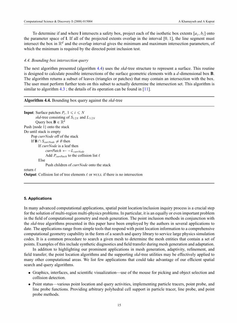
4.4. Bounding box intersection query

The next algorithm presented (algorithm 4.4) uses the skd-tree structure to represent a surface. This routineis designed to calculate possible intersections of the surface geometric elements with a d-dimensional box B.The algorithm returns a subset of leaves (triangles or patches) that may contain an intersection with the box.The user must perform further tests on this subset to actually determine the intersection set. This algorithm issimilar to algorithm 4.3 ; the details of its operation can be found in [11].

Algorithm 4.4. Bounding box query against the skd-tree

Input: Surface patches Pi , 1 6 i 6 Nskd-tree consisting of S1:2N and L1:2N

Query box B ∈ Rd

Push {node 1} onto the stackDo until stack is empty

Pop currNode off of the stackIf B ∩ ScurrNode 6= ∅ then

If currNode is a leaf thencurrPatch←−LcurrNode

Add PcurrPatch to the collision list `

ElsePush children of currNode onto the stack

return `

Output: Collision list of tree elements ` or null if there is no intersection

5. Applications

In many advanced computational applications, spatial point location/inclusion inquiry process is a crucial stepfor the solution of multi-region multi-physics problems. In particular, it is an equally or even important problemin the field of computational geometry and mesh generation. The point inclusion methods in conjunction withthe skd-tree algorithms presented in this paper have been employed by the authors in several applications todate. The applications range from simple tools that respond with point location information to a comprehensivecomputational geometry capability in the form of a search and query library to service large physics simulationcodes. It is a common procedure to search a given mesh to determine the mesh entities that contain a set ofpoints. Examples of this include synthetic diagnostics and field transfer during mesh generation and adaptation.

In addition to highlighting our prominent applications in mesh generation, adaptivity, refinement, andfield transfer; the point location algorithms and the supporting skd-tree utilities may be effectively applied tomany other computational areas. We list few applications that could take advantage of our efficient spatialsearch and query algorithms.

• Graphics, interfaces, and scientific visualization—use of the mouse for picking and object selection andcollision detection.

• Point status—various point location and query activities, implementing particle tracers, point probe, andline probe functions. Providing arbitrary polyhedral cell support in particle tracer, line probe, and pointprobe methods.

15

Computational Science & Discovery 1 (2008) 015004 A Khamayseh and A Kuprat

• Geometric processing—intersection, projection, computational topology, and ray casting.

• Mesh generation: point in body, adaptive mesh refinement, volume fraction calculation, advancing front,duplicate feature removal, material interface resolution (cell splitting) and mesh transformation.

• Multiphysics field transfer (or remapping): mapping a physics solution present on one mesh to another,topologically distinct mesh.

• Other physics applications—Monte Carlo, smooth particle hydrodynamics (SPH), hydrodynamic frontcollision, and front propagation methods.

The point in/out test is a query to determine if a particular set of domain coordinates lies inside or outsideof a body contained within the computational domain. Alternatively, this test may be viewed as a query todetermine which ‘part’ within the domain contains a particular location (if any). The mechanics of this test isbased on the particular representation of the domain geometry. Two models are possible.

1. If regions are defined in terms of b-rep parts that do not have an explicit relationship to some underlyingmesh discretizing the domain, it is necessary to use the part definition directly to determine the status ofthe query.

2. If the parts contained within the domain are explicitly associated with a computational mesh (e.g. a body-fitted mesh), the mesh elements contained within the body could share the spatial attributes associatedwith the body.

For the first case, only the basic part definition may be used to determine where a query point lies.The general problem, in this case, exists when the domain contains an arbitrary number of parts. Each part isassumed to be represented by some boundary definition; usually a list of surfaces (perhaps trimmed parametricsurfaces) that completely enclose the volume of the part. Further, the part definition is assumed to be airtight;the surfaces fit perfectly at seams such that there are no gaps or overlaps between surfaces and the volume iscompletely closed.

There are two possible states in which the query point may exist: (i) it is contained within one of the parts(that part, in turn, may be contained in another, and so on), or (ii) the location is outside of all the domain parts,in the interstitial region that separates the parts. In either case, to classify the status of the point (i.e. in or out)is to build the skd-tree of the parts or surfaces contained in the computational model. Thereafter, beginning atthe query point location, cast a ray in an arbitrary direction outward to the boundary of the problem domain todetermine whether the point is in or out using algorithm 3.1.

In the second case, where the model representation is associated with a mesh; the problem is significantlyless complex. It is only necessary to locate which mesh element contains the query point to know which part itis located in (or know that it is within the interstitial region). Such a spatial query requires a point-in-polyhedraquery test. To locate the query point in this case, the following steps are used:

1. Load the skd-tree with safety boxes enclosing the mesh elements.

2. Intersect the one-dimensional ray starting from the query point against the skd-tree.

3. Determine which element the query point lies in using algorithm 3.1, given the set of safety boxes returnedby the query.

This application requires a general spatial search if there is no a priori knowledge about the spatialrelationship of subsequent query locations (x, y, z). Often, these query locations may be spatially related; forexample, the first query may be a general query, but subsequent queries may involve points associated with theinitial query location (i.e. they may be the endpoint of a line that begins with the initial query point).

5.1. Hybrid mesh generation and adaptivity

One central application of the presented search and query capabilities is in the field of mesh generation. Ourmeshing efforts include the generation of polyhedral hybrid meshes with large number of elements that trulyrepresent complex multi-region geometries. These meshes provide more flexibility than traditional approaches

16

Computational Science & Discovery 1 (2008) 015004 A Khamayseh and A Kuprat

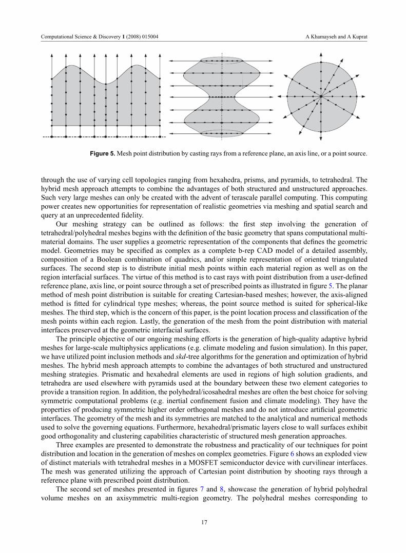
Figure 5. Mesh point distribution by casting rays from a reference plane, an axis line, or a point source.

through the use of varying cell topologies ranging from hexahedra, prisms, and pyramids, to tetrahedral. Thehybrid mesh approach attempts to combine the advantages of both structured and unstructured approaches.Such very large meshes can only be created with the advent of terascale parallel computing. This computingpower creates new opportunities for representation of realistic geometries via meshing and spatial search andquery at an unprecedented fidelity.

Our meshing strategy can be outlined as follows: the first step involving the generation oftetrahedral/polyhedral meshes begins with the definition of the basic geometry that spans computational multi-material domains. The user supplies a geometric representation of the components that defines the geometricmodel. Geometries may be specified as complex as a complete b-rep CAD model of a detailed assembly,composition of a Boolean combination of quadrics, and/or simple representation of oriented triangulatedsurfaces. The second step is to distribute initial mesh points within each material region as well as on theregion interfacial surfaces. The virtue of this method is to cast rays with point distribution from a user-definedreference plane, axis line, or point source through a set of prescribed points as illustrated in figure 5. The planarmethod of mesh point distribution is suitable for creating Cartesian-based meshes; however, the axis-alignedmethod is fitted for cylindrical type meshes; whereas, the point source method is suited for spherical-likemeshes. The third step, which is the concern of this paper, is the point location process and classification of themesh points within each region. Lastly, the generation of the mesh from the point distribution with materialinterfaces preserved at the geometric interfacial surfaces.

The principle objective of our ongoing meshing efforts is the generation of high-quality adaptive hybridmeshes for large-scale multiphysics applications (e.g. climate modeling and fusion simulation). In this paper,we have utilized point inclusion methods and skd-tree algorithms for the generation and optimization of hybridmeshes. The hybrid mesh approach attempts to combine the advantages of both structured and unstructuredmeshing strategies. Prismatic and hexahedral elements are used in regions of high solution gradients, andtetrahedra are used elsewhere with pyramids used at the boundary between these two element categories toprovide a transition region. In addition, the polyhedral/icosahedral meshes are often the best choice for solvingsymmetric computational problems (e.g. inertial confinement fusion and climate modeling). They have theproperties of producing symmetric higher order orthogonal meshes and do not introduce artificial geometricinterfaces. The geometry of the mesh and its symmetries are matched to the analytical and numerical methodsused to solve the governing equations. Furthermore, hexahedral/prismatic layers close to wall surfaces exhibitgood orthogonality and clustering capabilities characteristic of structured mesh generation approaches.

Three examples are presented to demonstrate the robustness and practicality of our techniques for pointdistribution and location in the generation of meshes on complex geometries. Figure 6 shows an exploded viewof distinct materials with tetrahedral meshes in a MOSFET semiconductor device with curvilinear interfaces.The mesh was generated utilizing the approach of Cartesian point distribution by shooting rays through areference plane with prescribed point distribution.

The second set of meshes presented in figures 7 and 8, showcase the generation of hybrid polyhedralvolume meshes on an axisymmetric multi-region geometry. The polyhedral meshes corresponding to

17

Computational Science & Discovery 1 (2008) 015004 A Khamayseh and A Kuprat

Figure 6. Exploded tetrahedral meshed regions of a MOSFET semiconductor device with curvilinearinterfaces.

individual material region are constructed using cylindrical and spherical point distribution type, respectively.The geometry of the mesh and its symmetries are matched to the analytical and numerical methods used tosolve the governing conservation equations. This type of meshing alleviates the problem degeneracy, say at thepoles; and preserves mesh smoothness, normal orthogonaliy and impedance (or mass) matching for preservingthe discrete accuracy of the simulation, both internal to the domain and near internal geometric interfaces.

5.2. Field transfer in coupled multiphysics

In addition to applications in mesh generation and refinement, the point location algorithms in conjunctionwith the skd-tree data structure presented in this study can be effectively applied to multiphysics solutiondata transfer. This process is often called remapping of physics field data from one donor source mesh toanother target recipient mesh, topologically distinct meshes. It is a common requirement in multiphysicsand adaptive analysis applications to transfer solution fields and their derivatives between meshes and/or toother applications. This process requires the evaluation of field variables and their derivatives at particulartarget locations, based on data associated with the donor mesh. For each target location, the solution transferprocess must (i) search and identify the mesh entities in the donor mesh from which data is required; (ii) queryand determine the spatial location of each target point on the donor mesh entities; (iii) compute the localisoparametric coordinates within the donor mesh for each of the target points; and (iv) evaluate the requiredfield components on the donor mesh at that location.

In some cases, the field may be preprocessed on the donor mesh to improve the accuracy of this data,and/or the level of continuity between mesh entities. Solution transfer is performed by integrating aspects ofspatial sort, search, query, interpolation of kernels (fields), and various implementations of geometry, mesh, andfield interfaces. Interpolation functions are required to support efficient field transfer operations that accountfor interacting meshes that are structured, unstructured, interfaced or overlapped and hybrid meshes.

We now present a case study of field remapping and transformation coupled with mesh adaptivityapplied to computational earth sciences and climate modeling. This study includes mapping of (lon-lat)orography field data across multiple planar/surface hybrid meshes. The initial non-smooth and irregularorography (satellite) data represents earth elevation height and considered an initial condition (atmospheredepth field and velocity) to the shallow-atmosphere computational model. Figure 9 shows a denseorography filed with (1 km) gridded resolution. The initial field data size was two gigabytes obtained fromhttp://www.ngdc.noaa.gov/mgg/topo/globe.html.

18

Computational Science & Discovery 1 (2008) 015004 A Khamayseh and A Kuprat

Figure 7. Exploded multi-material polyhedral mesh on an axialigned geometry.

Figure 8. Exploded multi-material hybrid volume mesh on a spherical-like geometry.

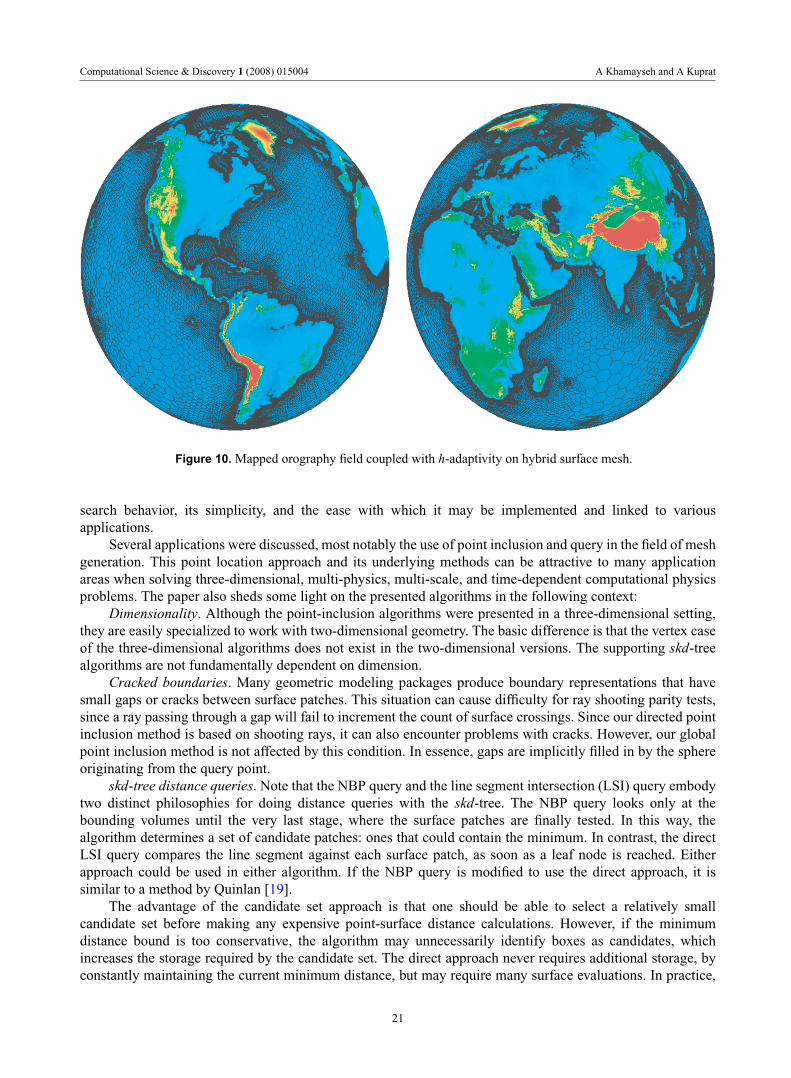
Orography plays an important role in determining the strength and location of the atmospheric jet streams.Its impact is most pronounced in the numerical simulation codes for the detailed regional climate studies.In addition, orography is a crucial parameter for prediction of many key climatic dynamics, elements, andmoisture physics, such as rainfall, snowfall and cloud cover. The phenomenon of climate variability is sensitiveto orographic effects which can be resolved by the generation of finer meshes in regions of high altitude. Wehave successfully introduced h-p adaptivity to a least-squares method with spherical harmonics basis functionsfor field mapping and mesh adaptation. The end mesh (figure 10) is much coarser at the sea level (50 km)and finer at the high altitude regions (1 km) with only a fraction of the original field data size. Moreover,the orography field was globally preserved to very small accuracy. The generation of adaptive meshes and the

19

Computational Science & Discovery 1 (2008) 015004 A Khamayseh and A Kuprat

Figure 9. Satellite data profile of earth elevation (top). Mapped orography field on h-adapted planarmesh (bottom).

smoothly mapped data for resolving orography field are used to approximate data field on the sphere for solvingclimate problems. In particular, field-based adaptive meshing approach proved best in finding differentiableapproximation of the orography field and computing the surface gradient of the mapped smoothed data.

Spatial search and query algorithms outlined in this paper are currently used in the geometry, meshing, andadaptivity efforts at Oak Ridge National Laboratory (ORNL), Pacific Northwest National Laboratory (PNNL),and Los Alamos National Laboratory (LANL). In addition, efforts are currently underway on integrating thesetools into the Interoperable Technologies for Advanced Petascale Simulations (ITAPS) library of Geometry,Mesh, Search and Query (GMSQ). The ITAPS center is one of the mathematics enabling technologies centersin the Department of Energy program on Scientific Discovery through Advanced Computing (SciDAC). Thepremise of the ITAPS technology focuses on developing advanced scalable interoperable software associatedwith geometry, mesh and field services. The center also provides integrated meshing/geometry tools forpartitioning and distributing the data for multiphysics applications.

6. Discussion

This paper develops a set of algorithms potentially useful for spatial search and query in various computationalapplications. Much of this paper focused on discussing the development of robust and efficient point inclusion(location) algorithms along with the skd-tree data structure. The skd-tree was introduced for its rapid general

20

Computational Science & Discovery 1 (2008) 015004 A Khamayseh and A Kuprat

Figure 10. Mapped orography field coupled with h-adaptivity on hybrid surface mesh.

search behavior, its simplicity, and the ease with which it may be implemented and linked to variousapplications.

Several applications were discussed, most notably the use of point inclusion and query in the field of meshgeneration. This point location approach and its underlying methods can be attractive to many applicationareas when solving three-dimensional, multi-physics, multi-scale, and time-dependent computational physicsproblems. The paper also sheds some light on the presented algorithms in the following context:

Dimensionality. Although the point-inclusion algorithms were presented in a three-dimensional setting,they are easily specialized to work with two-dimensional geometry. The basic difference is that the vertex caseof the three-dimensional algorithms does not exist in the two-dimensional versions. The supporting skd-treealgorithms are not fundamentally dependent on dimension.

Cracked boundaries. Many geometric modeling packages produce boundary representations that havesmall gaps or cracks between surface patches. This situation can cause difficulty for ray shooting parity tests,since a ray passing through a gap will fail to increment the count of surface crossings. Since our directed pointinclusion method is based on shooting rays, it can also encounter problems with cracks. However, our globalpoint inclusion method is not affected by this condition. In essence, gaps are implicitly filled in by the sphereoriginating from the query point.

skd-tree distance queries. Note that the NBP query and the line segment intersection (LSI) query embodytwo distinct philosophies for doing distance queries with the skd-tree. The NBP query looks only at thebounding volumes until the very last stage, where the surface patches are finally tested. In this way, thealgorithm determines a set of candidate patches: ones that could contain the minimum. In contrast, the directLSI query compares the line segment against each surface patch, as soon as a leaf node is reached. Eitherapproach could be used in either algorithm. If the NBP query is modified to use the direct approach, it issimilar to a method by Quinlan [19].

The advantage of the candidate set approach is that one should be able to select a relatively smallcandidate set before making any expensive point-surface distance calculations. However, if the minimumdistance bound is too conservative, the algorithm may unnecessarily identify boxes as candidates, whichincreases the storage required by the candidate set. The direct approach never requires additional storage, byconstantly maintaining the current minimum distance, but may require many surface evaluations. In practice,

21

Computational Science & Discovery 1 (2008) 015004 A Khamayseh and A Kuprat

we have found the candidate set approach, with an approximate ordering of candidates, to be the most efficientmethod.

Advantage of deterministic method. Our algorithms (2.1 and 3.1 supported by the skd-tree data structure)are currently in use in some existing mesh codes and they are competitive with other point inclusion algorithms.As applications, such as computational biology, geophysics and hydrodynamics, increasingly employ more andmore convoluted and complex meshes, it is more likely that rays cast from query points will intersect edges orvertices of the geometry (to within a given geometric tolerance). In extreme cases, methods that require cleanintersections of cast rays with the surface may bog down completely, and the advantage of the deterministicmethods we have presented will be increasingly realized.

Acknowledgments

The submitted manuscript has been authored by contractors of the US Government under contract no.DE-AC05-00OR22725. Accordingly, the US Government retains a non-exclusive, royalty-free license topublish or reproduce the published form of this contribution, or allow others to do so, for US Governmentpurposes.

© US Govt

References

[1] Bajaj C L and Dey T K 1992 Convex decomposition of polyhedra and robustness SIAM J. Comput. 21 339–64[2] Bærentzen J A and Aanæs H 2005 Signed distance computation using the angle weighted pseudonormal IEEE

Trans. Vis. Comp. Graphics 11 243–53[3] Chazelle B M and Dobkin D P 1980 Detection is easier than computation Proc. 12th ACM Symp. Theory of

Compututing (New York: ACM) pp 146–53 extended abstract[4] de Berg M, van Kreveld M, Overmars M and Schwarzkopf O 1997 Computational Geometry: Algorithms and

Applications (Berlin: Springer)[5] Dobkin D P and Kirkpatrick D G 1990 Determining the separation of preprocessed polyhedra—a unified approach

Proc. 17th Int. Colloq. Automata Lang. Program (Lecture Notes in Computer Science vol 443) (Berlin: Springer)pp 400–13

[6] Gottschalk S, Lin M C and Manocha D 1996 OBBTree: a hierarchical structure for rapid interference detectionProc. ACM SIGGRAPH ’96 pp 171–80

[7] Haines E 1994 Point in polygon strategies Graphics Gems IV ed P S Heckbert (New York: Academic) pp 24–46[8] Hoffmann C M 1997 Handbook of Discrete and Computational Geometry (Boca Raton, FL: CRC Press) chapter 47[9] Hubbard P M 1996 Approximating polyhedra with spheres for time-critical collision detection, ACM Trans. Gr. 15

179–210[10] Hui K C 1997 A robust point inclusion algorithm for regions bounded by parametric curve segments Computer-

Aided Design 29 771–8[11] Khamayseh A and Hansen G 2007 Use of the spatial kd-tree in computational physics applications Commun.

Comput. Phys. 2 545–76[12] Khamayseh A K, Kuprat A P and Henning P J 2003 Deterministic point inclusion methods for boundary

representation models Los Alamos National Laboratory Report LA-UR-03-2992[13] Knuth D E 1998 The Art of Computer Programming (vol 3) Searching and Sorting 2nd edn (Reading, MA:

Addison-Wesley)[14] Larsen E, Gottschalk S, Lin M C and Manocha D 1999 Fast proximity queries with swept sphere volumes Tech.

Report TR99-018, University of North Carolina, Chapel Hill, NC[15] Ooi B C 1990 Efficient Query Processing in Geographic Information Systems (Lecture Notes in Computer Science

vol 471) (Berlin: Springer)[16] O’Rourke J 1993 Computational Geometry in C (Cambridge: Cambridge University Press)[17] Preparata F P and Shamos M I 1985 Computational Geometry: An Introduction (New York: Springer)[18] Preparata F P and Tamassia R 1992 Efficient point location in a convex spatial cell-complex SIAM J. Comput. 21

267–80[19] Quinlan S 1994 Efficient distance computation between non-convex objects Proc. IEEE ICRA 1994, San Diego, CA

pp 602–7[20] Xavier P G 1996 A generic algorithm for constructing hierarchical representations of geometric objects Proc. IEEE

ICRA 1996 Minneapolis, MN 1996 4 3644–51

22