MPRAMunich Personal RePEc Archive

Determinants of Academic Attainment inthe US: a Quantile regression analysis oftest scores

Haile, Getinet and Nguyen, Ngoc Anh

Development and Policies Research Center (Hanoi) and

Policy Studies Institute (London)

2007

Online at http://mpra.ub.uni-muenchen.de/4626/

MPRA Paper No. 4626, posted 07. November 2007 / 04:04

[Paper under review by Education Economics]

Determinants of Academic Attainment in the US: a Quantile regression analysis of test scores

Getinet Astatike Haile∗ and Anh Ngoc Nguyen

Abstract We investigate the determinants of high school students’ academic attainment in maths, reading and science; focusing particularly on possible effects that ethnicity and family background may have on attainment. Using data from the NELS2000 and employing quantile regression techniques, we find two important results. First, the gaps in maths, reading and science test scores among ethnic groups vary across the conditional quantiles of the measured test scores. Specifically, Blacks and Hispanics tend to fare worse in their attainment at higher quantiles, particularly in science. Secondly, the effects of family background factors such as parental education and father’s occupation also vary across quantiles of the test score distribution. The implication of these findings is that the commonly made broad distinction on whether one is from a privileged/disadvantaged ethnic and/or family background may not tell the whole story that the academic attainment discourse has to note. Interventions aimed at closing the gap in attainment between Whites and minorities may need to target higher levels of the test score distribution. JEL Classification: I20, I21 Keywords: Educational attainment, Quantile regression, US

∗ Corresponding author: Getinet Haile, Policy Studies Institute, London W1W 6UP, UK; Tel: 44 2079117504; Fax: 44 2079117501; Email: haileg@psi.org.uk. Anh Nguyen would like to thank the ESRC for financial support.

2

1. Introduction

The educational attainment of individual students has been the focus of a large body

of empirical research (Hanushek 1986; Haveman and Wolfe 1995). There are several

reasons explaining the focus on educational attainment. First, there is a well

established link between education and how well a person succeeds in later life.

Numerous studies have pointed to the association between educational attainment and

post school earnings, employment and occupational status. Second, education is one

of the fundamental sources of long-term economic growth. The role of education on

economic growth and development is a topic of growing interest among economists

(Krueger and Lindahl 2001).

The bulk of the work related to modelling educational attainment is more or less

imbedded in the human capital theory and the household production model, which

were first introduced by Becker (1964) and later developed further by Leibowitz

(1994), Becker and Tomes (1979, 1986), Hanushek (1979, 1986). The educational

production function has become the main construct of the empirical literature to

identify the relative importance of measurable educational inputs. Analogous to firm

production, this framework relates contemporaneous child cognitive attainment with

the educational inputs from within the family as well as from the school. Most of the

previous empirical studies have estimated the education production model either by

using ordinary least squares (OLS) or ordinal logit/probit model depending on the

nature of data available. In these studies, a measure of educational attainment such as

test score is regressed on a range of explanatory variables [1].

3

While estimating how educational attainment is determined, “on average”, by various

explanatory variables is both useful and illuminating; it is quite possible that the

relationship between these explanatory variables and educational outcome of students

may differ across the distribution of students’ educational attainment. A natural and

relatively simple way to explore such differences across the distribution of students’

educational attainment is through quantile regression. By construction, quantile

regression answers the question of what is the marginal effect of an explanatory

variable at an arbitrary point on the conditional distribution of the dependent variable.

There are questions that can be addressed more fully by focusing on the tail of the

distribution rather than on the mean. In this paper, we are particularly interested in the

possible differences in the effect of ethnicity and family background across the

conditional quantiles of individual student’s academic attainment. As such, the

motivating question is whether the bottom of the distribution may systematically

differ from the top. Traditional techniques that focus on the effect of explanatory

variables on the mean are ill equipped to answer such questions.

A large gap in academic attainment (test scores) between white and black students in

the US has been documented in previous studies (Jencks and Phillips 1998; Cook and

Evans 2000; Krueger and Whitmore 2001; Fryer and Levitt 2002). The Black-White

test score gap has proven to be a remarkably robust empirical regularity, although the

gap has narrowed since 1970 (Cook and Evans 2000; Krueger and Whitmore 2001;

Huang and Hauser 2000; Hauser and Huang 1996). Even after controlling for a wide

range of covariates including family background and a measure of school inputs, a

substantial gap in test score persists (Huang and Hauser 2000) [2]. Possible

4

explanations for this gap include differences in family background and type of school

attended (Brooks-Gunn et al 1994; Cook and Evans 2000). This thread of research,

however, focused only on the differences between Black and White students at the

mean, neglecting potential differences across the distribution of test scores within

these groups. In addition, the possible differences between other ethnic groups, for

example Hispanics and Asian, remain largely unexplored. This study attempts to fill

these gaps in the existing research.

The main objectives of our paper are therefore to use the well-known US National

Educational Longitudinal Survey (NELS) to be able to: i/ extend the standard

empirical specification for students’ educational attainment using quantile regression

to explore possible differences in the explanatory power of a variety of determinants

of educational attainment across the conditional distribution of students’ academic

attainment and ii/ introduce further ethnic dimensions into the academic attainment

discourse which is dominated by distinctions between blacks and whites. The next

section of the paper presents the methodology and gives a further description of the

data used. Section 3 presents our estimation results and the final section concludes the

paper.

2. Methodology and data

If learning is the principal goal of education, then measures of scholastic attainment,

i.e. test scores, which involve a series of inputs, are the direct outcomes of the

educational process. The series of inputs into the educational process come not only

from the school attended but also from within the family. Hierarchical linear

5

modelling developed by Aitken and Longford (1986) has been used to model

educational attainment. This approach recognises the nested structure of the education

process, which is based on the assumption that students’ academic attainment are

influenced by the groups to which they belong. In an alternative approach, typically

taken by economists, educational attainment can be modelled within the framework of

educational production developed by Hanushek (1979, 1986, 1992). This approach

has been used extensively in empirical studies, most of which specify a variant of

educational production model in which students’ attainment (Yt) at time T is a

function of students’ previous attainment (Yt-1) and a vector of other covariates:

),( 1−= ttt YXfY (1)

As it stands equation (1) does not suggest linearity. However, applied work has often

assumed linear (or log-linear) functional form. This linearity assumption implies that

the effects of determinants are the same across the distribution of students’ academic

attainment. In our study, we follow the educational production approach but adopt the

quantile regression framework first developed by Koenker and Bassett (1978) to relax

the strict assumption of linearity in the effects of explanatory variables. Quantile

regression allows us to examine the effects of explanatory variables at different

quantiles of the test score distribution. Using this approach it is possible to estimate

models for a range of conditional quantile functions, including the conditional

median.

6

Similar to the estimation of the conditional mean regression, ,')|( βXxXYE ==

where β is obtained by solving 2' )(minargˆ βββ

∑ −=∈

iiR

Xyp

, the thθ quantile of the

conditional distribution of iy given X is defined as ),1,0(),()|( ' ∈= θθβθ ii XXyQ

where )|( XyQ iθ denotes the thθ quantile of the dependent variable conditioning on

the vector of covariates. As noted by Koenker and Bassett (1978), the estimation of

quantile regression is done by minimising the following equation:

{ } { }∑∑∑

∈<∈≥∈∈=−−+−

n

iRxyii

iixyii

iiR

uMinXyXyMink

iiii

k1::

' )(|'|)1(|| θθββββ

ρβθβθ (2)

where iy is the dependent variable, X is the vector of explanatory variables, β is

the vector of coefficients, θ is the quantile to be estimated, and (.)θρ is known as the

‘check function’ and defined as 0 )( ≥= iii uifuu θθθ θρθ and ii uu θθθ θρ )1()( −= if

0<iuθ . The minimisation problem can be solved by using linear programming

methods (Buchinsky, 1998). The coefficient vector may differ depending on the

particular quantile being estimated. This will allow us to examine (i) the differences in

academic attainment between ethnic groups at different quantile of the conditional

distribution of test scores after controlling for family background; and (ii) how the

effect of family background may vary across quantiles of the distribution of academic

attainment. By supplementing the estimation of the conditional mean functions with

the estimation of the conditional quantile functions, we expect to get a more complete

picture of the determination of students’ academic attainment.

As stated in the previous section, the data we use in this study is from the National

Educational Longitudinal Study (NELS 2000). The NELS, which began in 1988 with

7

a cross-sectional survey of eighth graders and which continued with four follow-up

interviews in 1990, 1992, 1994 and 2000, is a rich source of information on education

related variables. It provides detailed family background information, information on

students’ academic record as well as their high school experience. One important

feature of the NELS2000 is that various tests were administered to students before as

well as after they enter high school. This allows us to estimate the “value added” or

“growth” model of educational production function. Various measures of scholastic

outcome have been used by previous studies such as test score, dropout rates and

grade repetition. In this paper, we focus on standardised students’ test score in Maths,

Reading and Science as the dependent variables [3]. In addition to these test scores,

we also use a measure of composite test score in our study.

We concentrate first on differences between ethnic groups. As noted above, previous

studies have mostly investigated differences between black and white students (for

example, Krueger and Whitmore 2001). In this study, ethnic origin is observed for

five separate groups, namely non-Hispanic White, non-Hispanic Black, Hispanic and

Asian [4]. We are therefore able to investigate possible differences in academic

attainment of ethnic minority groups compared with white students, and how these

differences vary across the conditional distribution of test scores.

In addition to test scores, we have an extensive set of covariates to capture the effects

of family background, which are commonly found to be important in determining

attainment (Haveman and Wolfe 1995). They include parental education, parental

employment status, parental occupation, family size and family structure. Parental

education is often found to be very important in previous studies. Covariates on

8

family income, parental occupation and employment are used to control for the

availability of financial resources in the family which has been found to be important

determinant of academic attainment in previous studies (Hanushek 1992) [5]. Family

size is included since there is a trade-off between quantity and quality of children in

the household (Becker, 1991; Hanusheck 1992). Children are assumed to compete for

scarce resources within a family, i.e. parental time, financial and other resources.

Becker’s theory on the quantity and quality of children (Becker 1991; Becker and

Lewis 1973; Becker and Tomes 1976) suggests that the time parents allocate to each

child is decreasing with the number of siblings. In addition, researchers have found

that family structure plays a critical role (Mare 1980; Astone et al 1991; Manski et al

1992; Haveman et al 1991; Evans et al 1992) [6]. The presence of both parents in the

family home and the financial resources contributed by them explain, at least in part,

the benefit that students from intact families may reap. Findings from empirical

studies tend to lend support to the above hypotheses [7].

3. Empirical results and discussion

We have estimated quantil regressions separately for males and females at the 0.1,

0.25, 0.5, 0.75 and 0.9 quantiles. The estimation results obtained are presented in

Tables 2 – 7. As well as the quantile regressions, we estimate conditional mean

regressions in each case to be able to compare the two and to make comparisons with

findings in the literature handy. Our discussion focuses on differences between ethnic

groups across the conditional distribution of maths, reading and science test scores

and the effect of ethnicity and family background factors on academic attainment as

measured by test scores. Table 1 reports mean values of test scores in maths, reading

9

and science separately for males and females for each of the four ethnic groups

considered. The Table shows that there are noticeable differences among ethnic

groups in terms of academic attainment in the three subjects. Irrespective of gender,

Black and Hispanic students perform worse than their white and Asian counterparts

across the three subjects.

Our findings from the mean regressions reported in the first columns of Tables 2-7 are

in line with those obtained by previous studies. Previous attainment is generally found

to be significant determinant of (current) attainment in the three subjects, and this

finding holds across all equations we have estimated. Controlling for a range of other

factors, differences between ethnic groups remain to be statistically significant. Black

students, both males and females, are found to perform worse than their White

counterparts in all three subjects. Hispanic students are the next worse performers

when compared with White students. This pattern holds across the three subjects for

male Hispanic students but is restricted to attainment in science for females. There is

some evidence that Asian students perform better than White students in maths and

science but not in reading. In particular, Asian female students perform better than

their White counterparts in maths and science while Asian males do so only in maths

and marginally at that. In line with previous studies, we find that family background

factors such as parental education and occupation are important determinants of

students’ academic attainment across all equations we estimate as can be gathered

from the statistically significant coefficients relating to these characteristics.

The estimation results from the quantile regressions largely mimic those from the

mean regressions in terms of statistical significance but do indicate marked variations

10

in the observed effects across the quantiles we have estimated. The Black-White gap

in maths, reading and science test scores are found to be statistically significant and

more profound at higher quantiles of the conditional maths, reading and science test

scores than at the lower quantiles. These are findings that the mean regression results

reported in the first columns are unable to discern. The implication of this finding is

that when designing measures that are meant to close the Black-White gap, the focus

of any intervention should be targeted at higher levels of the test score distribution.

This is because at lower level of the test score distribution there does not exist a

statistically significant gap in attainment particularly with regards to maths and

reading test scores.

Looking at the results for other ethnic groups, we find that there are some differences

between the mean and quantile regression estimates. In contrast to results from the

mean regressions, Asian male students are only found to perform better than their

White counterparts in maths test only at the 0.9 quantile. On the other hand, Asian

female students are found to perform better than their White counterparts across all

quantiles as can be seen from the results at the 0.25, 0.5, 0.75 and 0.9 quantiles. In

reading, Asian males are not found to perform significantly differently to their White

counterparts. This is a finding that is corroborated by results from both the mean and

quantile regressions, excepting the result at the median quantile. Asian female

students, on the other hand, are statistically indistinguishable from their White peers

in terms of attainment in reading, which is in line with findings from the mean

regression. Our findings for Hispanics are similar to mean regression. In particular,

Hispanic male and female students are found to be performing worse than their white

counterparts around the median. In a similar fashion to Blacks, the gap between

11

Hispanics and Whites in science widens with the quantiles. Thus, at higher quantiles

the Hispanics-White gap is the greatest and these findings hold both for males and

females. In contrast, Asian males are not found to be significantly different in terms of

attainment in science, while Asian females perform better than Whites particularly at

higher quantiles.

With respect to the effect of family background factors, several interesting findings

are worth noting. First, similar to mean regression parental education is very

important. However, the effects of parental education on children’s maths, reading

and science test scores vary across the quantiles. With regards to maths scores, the

effect of parental education is stronger for both males and females. This effect of

parental education is stronger for males at higher quantiles while for females the

effect appears to be stronger at lower quantiels. The same pattern emerges regarding

the effect of parental education on reading scores of both males and females. In

contrast, the effect of parental education on attainment in science is found to be

similar for both males and females where it has stronger effects at higher quantiles.

Father’s occupation is found to have significant effect on attainment for female

students in the three subjects considered but the effect on male students is not found

to be as important. For female students, having father in high occupational status

(professional/managerial) improves their test score at the median and the surrounding

0.25 and 0.75 quantiles, but not at the other quantiles. This finding is in sharp contrast

to previous studies that mostly rely on mean regression. That father’s occupation is

found to have no effect on students’ attainment at the higher quantile may mean that

12

for well-performing students family financial resources as captured by father’s

occupation may not be too importance.

4. Conclusion

In this paper, we investigate the differences in academic attainment across ethnic

groups and the effect of family background factors on educational attainment. Using

data from the National Educational Longitudinal Study (NELS 2000) and employing

quantile regression techniques, we identify several interesting findings that previous

research which relies on mean regression has not brought to light. In particular, we

find that the gap in attainment in maths, reading and science tests between ethnic

groups is found to vary across the conditional quantiles of the measured test scores,

widening at higher quantiles. Our findings for the gap between Black and White as

well as Hispanics and White students in test scores from the three subjects suggest

that interventions that are meant to reduce such gaps in academic attainment among

these ethnic groups should take into account the relative location of students in the

test score distribution. Measures meant to close any attainment gap among ethnic

groups should be targeted at higher levels of the test score distribution for that is

where these gaps are at their maximum.

13

References Aitken, M. and N. Longford (1986) Statistical Modelling in School Effectiveness

Studies, Journal of the Royal Statistical Society, Series A, 149, pp. 1-43.

Astone, M. and S. McLanahan (1991) Family Structure, Parental Practices, and High

School Completion, American Sociological Review, 56, pp. 309-320.

Becker, G (1991) A Treatise on the Family Cambridge, Massachusetts: Harvard

University Press.

Becker, G and H. Lewis (1973) On the Interaction between the Quantity and Quality

of Children, Journal of Political Economy, 81 (2), pp.s279-s288.

Becker, G. and N. Tomes (1976) Child Endowments and the Quantity and Quality of

Children, Journal of Political Economy, 84 (4), pp. 143-162.

Becker, G. and N. Tomes (1979) An Equilibrium Theory of the Distribution of

Income and Intergenerational Mobility, Journal of Political Economy, 87 (6),

pp.1153-1186.

Becker, G. and N. Tomes (1986) Human Capital and the Rise and Fall of Families,

Journal of Labour Economics, 4 (3), pp. 1-39.

Becker, Gary S. (1964) Human Capital: A Theoretical and Empirical Analysis, with

Special Reference to Education, New York: National Bureau of Economic Research.

Brooks-Gunn, J., R. Gross, P. Klebanov, C. McCarton, M. McCormick, R. Breadley

and D. Scott (1994) Effects of Early Educational Intervention in Families, Who Do

and Who Do Not Receive Welfare: The Infant Health and Development Program,

14

Paper presented at research briefing, Board on Children and Families, December 5-6,

1994, Teachers College, Columbia University.

Buchinsky, M (1998) Recent advances in quantile regression models: A practical

guide for empirical research, Journal of Human Resources, 3, pp. 88-126.

Cook, M and W. Evans (2000) Families or schools? Explaining the convergence in

White and Black academic performance, Journal of Labor Economics, 18, pp. 729-

754.

Fryer, R. and S. Levitt (2002) Understanding the Balck-White test score gap in the

first two years of school, mimeo, NBER.

Hanushek, E. (1979) Conceptual and Empirical Issues in the Estimation of

Educational Production Functions, Journal of Human Resources, 14 (3), pp. 351-388.

Hanushek, E. (1986) The Economics of Schooling: Production and Efficiency in

Public Schools, Journal of Economic Literature, 24 (3), pp. 1141-1177.

Hanushek, E. (1992) The Trade-off Between Child Quantity and Quality, Journal of

Political Economy, 100 (1), pp. 84-117.

Hauser, R. and M. Huang (1996) Trends in Black-White test-score differentials,

mimeo, Institute for Research on Poverty, University of Wisconsin-Madison.

Haveman, R. and B. Wolfe (1995) The Determinants of Children’s Attainments: A

Review of Methods and Findings, Journal of Economic Literature, 33 (4), pp. 1829-

1878.

Haveman, R., B. Wolfe and J. Spaulding (1991) Childhood Events and Circumstances

Influencing High School Completion, Demography, 28 (1), pp. 133-157.

Huang, M. and R. Hauser (2000) Convergent trends in Black-White differentials in

the US: A Correction of Richard Lynn, mimeo, Institute for Research on Poverty,

University of Wisconsin-Madison.

15

Janson, W. and D. Neal (1998) Basic skills and the Black-White earnings gap, in

Jencks and Phillips (eds.) The Black-White Test Score Gap, Washington DC:

Brookings Institution Press.

Jencks, C. & M. Phillips (1998). The Black-White Test Score Gap Brookings

Institution Press

Jonsson, J. and Gahler, M. (1997) Family Dissolution, Family Reconstruction, and

Children’s Educational Careers: Recent Evidence from Sweden, Demography, 34(2),

pp. 277-293

Koenker, R and G. Bassett (1978) Regression quantiles, Econometrica, 46, pp. 33-50.

Krueger, A. and D. Whitmore (2001) Would Smaller Classes Help Close the Black-

White Achievement Gap? Working Paper #451, Princeton University,

http://www.irs.princeton.edu/pubs/pdfs/451.pdf

Krueger, A. and M. Lindahl (2001) Education for Growth: Why and for whom?

Journal of Economic Literature, 39 (4), pp. 1101-1136.

Leibowitz, A. (1974) Home Investment in Children, Journal of Political Economy, 82

(2), pp. 111-131.

Manski, C. F., G. D. Sandufer, S. McLanahan and D. Powers (1992) Alternative

Estimates of the Effect of Family Structure During Adolescence on High School

Graduation, Journal of The American Statistical Association, 87 (417), pp. 25-37.

Mare, R. D. (1980) Social Background and School Continuation Decisions, American

Statistical Association, 75, pp. 295-305

McLanahan, S. (1985) Family Structure and the Reproduction of Poverty, American

Journal of Sociology, 90 (4), pp. 873-901

Ribar, David C. (1994) Teenage Fertility and High School Completion, The Review of

Economics & Statistics, 76 (3), pp. 413-24.

16

Sander W. and A. Krautmann (1995) Catholic schools, dropout rates and educational

attainment, Economic Inquiry, 33, pp. 217-233.

Sander, W. (2001) The effects of Catholic schools on religiosity, education, and

competition, mimeo, Teachers College, Columbia University.

Smith, S. (1999) Do Better Schools Matter? Parental valuation of elementary

education, Quarterly Journal of Economics, May 1999, pp. 577-599.

Vartanian, T. and P. Gleason (1999) Do Neighbourhood Conditions Affect High

School Dropout and College Graduation Rates, Journal of Socioeconomics, 28, pp.

21-42.

17

Table 1: Attainment by Ethnicity

Maths Reading Science

Males Females Males Females Males Females

White 52.5 53.4 53.3 52 54 52

(9.5) (9.8) (9.2) (10.0) (10.5) (9.3)

No. 3625 3281 3661 3275 3637 4027

Black 45.7 45.3 47.8 45.2 46 46

(9.1) (8.8) (9.4) (10.1) (8.6) (8.0)

No. 418 357 482 355 418 559

Asian 57.1 56.8 55 53 55 52

(9.4) (10.2) (9.1) (10.2) (10.9) (9.7)

No. 329 32 331 324 361 384

Hispanic 46.3 47.6 48.2 46.6 48 46

(8.7) (9.2) (9.0) (9.2) (9.2) (7.8)

No. 635 533 635 533 606 747 Note: Standard deviations in parenthesis

18

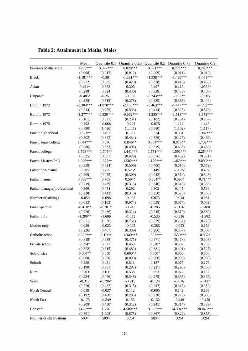
Table 2: Attainment in Maths, Males

Mean Quantile 0.1 Quantile 0.25 Quantile 0.5 Quantile 0.75 Quantile 0.9 Previous Maths score 0.795*** 0.827*** 0.828*** 0.821*** 0.771*** 0.700*** (0.008) (0.017) (0.012) (0.009) (0.011) (0.012) Black -1.181*** -0.301 -1.231*** -1.538*** -1.439*** -1.461*** (0.272) (0.585) (0.420) (0.328) (0.416) (0.455) Asian 0.491* 0.662 0.306 0.407 0.415 1.033** (0.289) (0.594) (0.436) (0.339) (0.433) (0.467) Hispanic -0.485* -0.251 -0.550 -0.743*** -0.652* -0.305 (0.255) (0.515) (0.373) (0.289) (0.368) (0.404) Born in 1972 -3.304*** -1.870*** -2.458*** -3.463*** -4.447*** -4.992*** (0.314) (0.725) (0.533) (0.414) (0.525) (0.578) Born in 1973 -1.277*** -0.820*** -0.962*** -1.285*** -1.518*** -1.372*** (0.161) (0.321) (0.231) (0.182) (0.234) (0.257) Born in 1975 0.492 -0.068 -0.293 -0.076 1.122 1.426 (0.790) (1.426) (1.111) (0.880) (1.102) (1.117) Parent high school 0.621** 0.497 0.173 0.374 0.381 1.387*** (0.302) (0.622) (0.434) (0.339) (0.427) (0.462) Parent some college 1.044*** 0.636 0.846** 0.934*** 0.976** 1.739*** (0.286) (0.583) (0.405) (0.319) (0.405) (0.438) Parent college 1.798*** 1.745** 1.441*** 1.571*** 1.591*** 2.254*** (0.335) (0.687) (0.479) (0.376) (0.482) (0.521) Parent Masters/PhD 1.806*** 1.677** 1.582*** 1.176*** 1.469*** 2.096*** (0.359) (0.724) (0.506) (0.400) (0.516) (0.572) Father non-manual 0.305 0.725 0.525* 0.149 -0.075 0.407 (0.209) (0.425) (0.309) (0.243) (0.314) (0.343) Father manual 0.596*** 0.705 0.564* 0.564** 0.596* 0.714** (0.219) (0.439) (0.315) (0.246) (0.313) (0.336) Father manager/professional 0.369 0.434 0.292 0.302 0.445 0.594 (0.228) (0.442) (0.316) (0.250) (0.328) (0.365) Number of siblings -0.050 -0.098 -0.098 -0.075 -0.014 0.081 (0.052) (0.103) (0.074) (0.058) (0.074) (0.082) Parent-partner -0.410** -0.781* -0.245 -0.285 -0.176 -0.408 (0.226) (0.436) (0.314) (0.245) (0.310) (0.339) Father only -1.299** -1.689 -1.055 -0.535 -0.516 -1.282 (0.551) (1.036) (0.751) (0.579) (0.737) (0.773) Mother only 0.029 -0.023 -0.025 -0.385 -0.053 0.159 (0.226) (0.467) (0.339) (0.266) (0.337) (0.360) Catholic school 1.352*** 1.166* 1.349*** 1.587*** 1.550*** 0.962* (0.318) (0.638) (0.471) (0.371) (0.478) (0.507) Private school 0.594* 0.571 0.453 0.670* 0.502 0.203 (0.322) (0.615) (0.482) (0.381) (0.491) (0.527) School size 0.000** 0.000 0.000** 0.000* 0.000 0.000 (0.000) (0.000) (0.000) (0.000) (0.000) (0.000) Suburb 0.220 0.421 0.511 0.187 0.077 0.176 (0.190) (0.381) (0.287) (0.227) (0.290) (0.306) Rural 0.203 0.166 0.538 0.253 0.077 0.152 (0.234) (0.446) (0.348) (0.275) (0.355) (0.367) West -0.312 -0.796* -0.215 -0.124 -0.076 -0.437 (0.220) (0.432) (0.315) (0.247) (0.317) (0.352) North Central 0.059 -0.037 0.112 -0.095 0.142 0.199 (0.192) (0.400) (0.285) (0.220) (0.279) (0.300) North East -0.173 -0.249 0.155 -0.152 -0.449 -0.426 (0.209) (0.430) (0.312) (0.245) (0.314) (0.339) Constant 9.473*** 1.776 4.500*** 8.525*** 14.304*** 20.049*** (0.591) (1.205) (0.875) (0.667) (0.822) (0.855) Number of observations 5094 5094 5094 5094 5094 5094

19

R2/Pseudo R2 0.81 0.52 0.58 0.59 0.57 0.53 Note: Standard errors are in parentheses; * significant at 10%; ** significant at 5%; *** significant at 1%. Table 3: Attainment in Maths, Females

Mean Quantile 0.1 Quantile 0.25 Quantile 0.5 Quantile 0.75 Quantile 0.9 Previous Maths score 0.818*** 0.819*** 0.839*** 0.838*** 0.805*** 0.776*** (0.007) (0.015) (0.011) (0.009) (0.010) (0.011) Black -0.792*** 0.036 -0.599* -1.111*** -1.051*** -0.827** (0.221) (0.424) (0.327) (0.286) (0.351) (0.411) Asian 0.804*** 0.422 0.646* 0.848*** 1.080*** 1.067*** (0.269) (0.501) (0.379) (0.331) (0.395) (0.456) Hispanic -0.338 -0.301 -0.651** -0.368 -0.363 -0.159 (0.213) (0.411) (0.312) (0.269) (0.324) (0.372) Born in 1972 -3.544*** -2.438*** -2.437*** -3.440*** -4.328*** -5.385*** (0.380) (0.748) (0.577) (0.502) (0.609) (0.706) Born in 1973 -0.981*** -0.959*** -0.778*** -0.875*** -1.142*** -0.879*** (0.149) (0.280) (0.208) (0.182) (0.221) (0.257) Born in 1975 0.784 -0.108 0.578 0.417 0.743 0.326 (0.577) (1.210) (0.882) (0.777) (0.925) (1.102) Parent high school 0.358 0.169 0.473 0.367 0.466 0.276 (0.245) (0.452) (0.344) (0.297) (0.355) (0.411) Parent some college 1.132*** 0.604 0.966*** 1.047*** 1.349*** 1.281*** (0.233) (0.437) (0.327) (0.281) (0.333) (0.384) Parent college 1.669*** 1.291*** 1.345*** 1.665*** 1.568*** 1.497*** (0.285) (0.547) (0.399) (0.346) (0.418) (0.482) Parent Masters/PhD 1.647*** 2.272*** 1.596*** 1.424*** 1.273*** 1.103*** (0.299) (0.605) (0.435) (0.377) (0.451) (0.518) Father non-manual 0.363** 0.325 0.783*** 0.535** 0.128 -0.269 (0.184) (0.354) (0.264) (0.228) (0.274) (0.319) Father manual 0.374** 0.348 0.649*** 0.449** 0.172 -0.127 (0.182) (0.349) (0.260) (0.226) (0.271) (0.313) Father Professional/manager 0.448** 0.792** 0.677** 0.393* 0.283 -0.160 (0.191) (0.363) (0.266) (0.235) (0.287) (0.336) Number of siblings -0.006 -0.079 -0.053 -0.031 0.029 0.061 (0.041) (0.077) (0.060) (0.052) (0.061) (0.072) Parent-partner -0.559*** -0.254 -0.621*** -0.379* -0.567** -0.610* (0.183) (0.342) (0.257) (0.225) (0.271) (0.317) Father only 0.050 0.059 0.091 0.173 0.244 -0.181 (0.623) (1.002) (0.770) (0.677) (0.812) (0.854) Mother only 0.030 -0.267 -0.148 0.408 0.408 -0.201 (0.197) (0.376) (0.276) (0.240) (0.290) (0.342) Catholic school 0.125 0.300 0.337 -0.148 -0.048 0.174 (0.273) (0.542) (0.416) (0.359) (0.423) (0.503) Private school -0.034 0.480 -0.138 -0.032 -0.118 -0.273 (0.287) (0.587) (0.434) (0.379) (0.455) (0.546) School size 0.000** 0.000 0.000** 0.000** 0.000 0.000 (0.000) (0.000) (0.000) (0.000) (0.000) (0.000) Suburb -0.278* -0.286 -0.176 -0.364* -0.347 -0.270 (0.167) (0.327) (0.244) (0.212) (0.255) (0.302) Rural -0.385* -0.337 -0.658 -0.583** -0.245 -0.554 (0.198) (0.381) (0.289) (0.252) (0.302) (0.350) West -0.300 -0.098 -0.391 -0.308 -0.164 0.068 (0.189) (0.350) (0.265) (0.233) (0.284) (0.333) North Central -0.112 0.020 -0.264 -0.193 -0.232 0.191 (0.162) (0.310) (0.234) (0.205) (0.246) (0.286) North East -0.017 -0.103 -0.170 0.147 0.135 -0.327 (0.183) (0.352) (0.263) (0.230) (0.278) (0.320) Constant 8.934*** 3.612*** 5.443*** 8.209*** 12.462*** 16.719*** (0.476) (0.934) (0.730) (0.618) (0.703) (0.785) Number of observations 5094 5094 5095 5094 5094 5095

20

R2/Pseudo R2 0.81 0.52 0.58 0.59 0.57 0.53 Note: Standard errors are in parentheses; * significant at 10%; ** significant at 5%; *** significant at 1%. Table 4: Attainment in reading, Males

Mean Quantile 0.1 Quantile 0.25 Quantile 0.5 Quantile 0.75 Quantile 0.9 Previous reading score 0.736*** 0.706*** 0.767*** 0.782*** 0.742*** 0.651*** (0.010) (0.020) (0.013) (0.010) (0.014) (0.016) Black -1.300*** -0.549 -0.950** -1.253*** -2.055*** -1.691*** (0.343) (0.734) (0.472) (0.369) (0.546) (0.638) Asian 0.501 -0.635 0.480 0.800** 0.672 0.620 (0.387) (0.745) (0.488) (0.381) (0.563) (0.675) Hispanic -0.903*** -0.524 -0.821* -1.221*** -0.623 -0.585 (0.316) (0.658) (0.421) (0.326) (0.473) (0.560) Born in 1972 -2.880*** -2.196** -2.115*** -2.474*** -4.101*** -3.705*** (0.406) (0.919) (0.593) (0.463) (0.678) (0.817) Born in 1973 -1.410*** -1.698*** -1.505*** -1.403*** -1.403*** -1.147*** (0.199) (0.407) (0.263) (0.205) (0.306) (0.363) Born in 1975 1.006 1.224 0.981 0.696 0.405 1.400 (0.933) (1.764) (1.248) (0.994) (1.446) (1.613) Parent high school 0.582 0.228 -0.060 0.361 1.254** 1.071 (0.358) (0.768) (0.489) (0.383) (0.565) (0.682) Parent some college 0.904*** 0.334 0.523 0.871** 1.729*** 1.415** (0.341) (0.730) (0.460) (0.361) (0.536) (0.648) Parent college 1.597*** 1.228 1.343** 1.019** 2.031*** 2.270*** (0.411) (0.872) (0.548) (0.426) (0.637) (0.772) Parent Masters/PhD 2.096*** 2.967*** 1.985*** 1.464*** 2.080*** 2.410*** (0.425) (0.885) (0.570) (0.451) (0.681) (0.818) Father non-manual 0.629** 0.386 0.423 0.976*** 0.546 0.180 (0.262) (0.551) (0.351) (0.274) (0.404) (0.483) Father manual 0.481* -0.125 0.092 0.639** 0.649 0.863 (0.268) (0.553) (0.356) (0.278) (0.411) (0.484) Father Professional/manager 0.544** -0.203 0.480 0.824*** 0.840** 0.351 (0.275) (0.534) (0.354) (0.282) (0.424) (0.506) Number of siblings -0.029 -0.012 0.057 -0.016 0.028 -0.036 (0.064) (0.129) (0.083) (0.065) (0.096) (0.118) Parent-partner -0.422 -0.647 -0.292 -0.572** -0.507 -0.463 (0.266) (0.531) (0.353) (0.277) (0.409) (0.481) Father only -0.617 -0.517 -0.708 -0.664 -0.685 -0.287 (0.650) (1.291) (0.845) (0.657) (0.966) (1.173) Mother only -0.452 -0.594 -0.668 -0.277 -0.663 -0.542 (0.285) (0.579) (0.383) (0.299) (0.446) (0.538) Catholic school 0.768* 0.314 1.266** 1.353*** 0.613 -0.376 (0.395) (0.808) (0.526) (0.422) (0.637) (0.753) Private school 1.466*** 2.340*** 2.094*** 1.359*** 1.540** 0.864 (0.415) (0.809) (0.539) (0.429) (0.647) (0.785) School size 0.000 0.000 0.000 0.000* 0.000 0.000 (0.000) (0.000) (0.000) (0.000) (0.000) (0.000) Suburb 0.042 -0.130 0.081 0.559** 0.193 -0.080 (0.243) (0.490) (0.326) (0.257) (0.380) (0.453) Rural -0.246 -0.488 0.117 0.309 -0.205 -0.525 (0.295) (0.583) (0.394) (0.312) (0.465) (0.554) West -0.645** -0.817 -0.780** -0.589** -1.036** -0.237 (0.278) (0.545) (0.352) (0.278) (0.416) (0.501) North Central -0.235 -0.087 -0.130 -0.232 -0.520 -0.708* (0.237) (0.490) (0.319) (0.248) (0.363) (0.428) North East -0.232 -0.018 -0.287 -0.134 -0.511 -0.579 (0.262) (0.550) (0.357) (0.277) (0.411) (0.484) Constant 12.711*** 7.350*** 7.511*** 9.946*** 15.843*** 24.789*** (0.703) (1.447) (0.961) (0.745) (1.040) (1.272) Number of observations 4490 4490 4490 4490 4490 4490

21

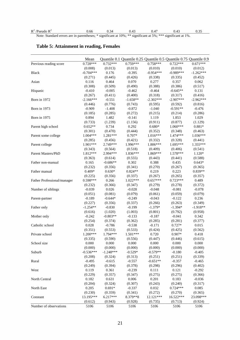
R2 /Pseudo R2 0.66 0.34 0.43 0.47 0.43 0.35 Note: Standard errors are in parentheses; * significant at 10%; ** significant at 5%; *** significant at 1%. Table 5: Attainment in reading, Females

Mean Quantile 0.1 Quantile 0.25 Quantile 0.5 Quantile 0.75 Quantile 0.9 Previous reading score 0.728*** 0.732*** 0.759*** 0.758*** 0.722*** 0.671*** (0.008) (0.013) (0.013) (0.010) (0.010) (0.012) Black -0.704*** 0.176 -0.395 -0.954*** -0.989*** -1.262*** (0.271) (0.445) (0.426) (0.338) (0.335) (0.452) Asian 0.116 0.464 0.070 0.277 0.357 0.062 (0.308) (0.509) (0.490) (0.388) (0.386) (0.517) Hispanic -0.410 -0.005 -0.462 -0.464 -0.645** 0.131 (0.267) (0.411) (0.400) (0.318) (0.317) (0.416) Born in 1972 -2.166*** -0.551 -1.658** -2.302*** -2.907*** -2.962*** (0.446) (0.776) (0.743) (0.595) (0.592) (0.816) Born in 1973 -0.909 -1.408 -0.872 -1.040 -0.591** -0.476 (0.185) (0.285) (0.272) (0.215) (0.214) (0.286) Born in 1975 0.894 1.482 -0.141 1.119 1.853 1.029 (0.733) (1.239) (1.156) (0.911) (0.877) (1.129) Parent high school 0.652** 0.734 0.292 0.680* 1.060*** 0.881* (0.301) (0.470) (0.444) (0.352) (0.348) (0.463) Parent some college 1.004*** 1.281*** 0.707* 1.016*** 1.474*** 1.036*** (0.285) (0.456) (0.421) (0.332) (0.328) (0.441) Parent college 1.901*** 2.749*** 1.996*** 1.806*** 1.695*** 1.355*** (0.343) (0.564) (0.518) (0.409) (0.406) (0.541) Parent Masters/PhD 1.812*** 2.994*** 1.836*** 1.869*** 1.578*** 1.120* (0.363) (0.614) (0.555) (0.443) (0.441) (0.588) Father non-manual 0.165 -0.686** 0.302 0.388 0.435 0.643* (0.232) (0.356) (0.341) (0.270) (0.267) (0.365) Father manual 0.409* 0.630* 0.824** 0.219 0.223 0.839** (0.225) (0.356) (0.337) (0.267) (0.265) (0.357) Father Professional/manager 0.598*** 0.266 1.022*** 0.657*** 0.723*** 0.489 (0.232) (0.366) (0.347) (0.279) (0.278) (0.372) Number of siblings -0.039 0.026 -0.028 -0.048 -0.081 -0.078 (0.051) (0.081) (0.079) (0.061) (0.059) (0.079) Parent-partner -0.189 -0.644* -0.249 -0.043 -0.122 0.236 (0.227) (0.356) (0.337) (0.266) (0.263) (0.349) Father only -1.254** -0.830 -0.199 -1.379* -1.394* -1.918** (0.616) (1.020) (1.003) (0.801) (0.792) (0.958) Mother only -0.242 -0.803** -0.133 -0.187 -0.041 0.342 (0.254) (0.374) (0.362) (0.285) (0.281) (0.377) Catholic school 0.028 -0.786 -0.538 -0.171 0.727* 0.015 (0.351) (0.553) (0.533) (0.424) (0.425) (0.562) Private school 1.200*** 1.794*** 1.501*** 0.720 0.907* 0.418 (0.335) (0.590) (0.556) (0.447) (0.446) (0.615) School size 0.000 0.000 0.000 0.000 0.000 0.000 (0.000) (0.000) (0.000) (0.000) (0.000) (0.000) Suburb -0.536*** -1.248*** -0.529* -0.579** -0.180 -0.405 (0.208) (0.324) (0.313) (0.251) (0.251) (0.339) Rural -0.495 -0.615 -0.557 -0.651** -0.357 -0.465 (0.249) (0.394) (0.378) (0.298) (0.296) (0.402) West 0.119 0.361 -0.239 0.111 0.121 -0.292 (0.229) (0.357) (0.347) (0.275) (0.275) (0.366) North Central 0.182 0.631 0.006 0.201 0.183 -0.036 (0.204) (0.324) (0.307) (0.243) (0.240) (0.317) North East 0.205 0.691* -0.337 0.032 0.724*** 0.085 (0.230) (0.359) (0.341) (0.272) (0.270) (0.365) Constant 13.195*** 6.217*** 8.379**8 12.121*** 16.522*** 23.098*** (0.612) (0.943) (0.928) (0.735) (0.713) (0.924) Number of observations 5106 5106 5106 5106 5106 5106

22

R2/Pseudo R2 0.68 0.41 0.47 0.48 0.44 0.37 Note: Standard errors are in parentheses; * significant at 10%; ** significant at 5%; *** significant at 1%. Table 6: Attainment in science, Males

Mean Quantile 0.1 Quantile 0.25 Quantile 0.5 Quantile 0.75 Quantile 0.9 Previous science score 0.638*** 0.646*** 0.713*** 0.682*** 0.623*** 0.544*** (0.011) (0.021) (0.012) (0.014) (0.012) (0.015) Black -3.720*** -2.613*** -2.740*** -3.957*** -3.744*** -4.975*** (0.371) (0.802) (0.471) (0.521) (0.480) (0.574) Asian 0.401 1.124 0.214 -0.008 0.753 0.235 (0.431) (0.811) (0.479) (0.537) (0.499) (0.597) Hispanic -1.981*** -1.128 -1.904*** -2.120*** -1.778*** -1.937*** (0.348) (0.729) (0.419) (0.458) (0.417) (0.496) Born in 1972 -3.657*** -1.928* -3.118*** -3.242*** -3.769*** -4.449*** (0.470) (0.999) (0.590) (0.651) (0.596) (0.714) Born in 1973 -1.035*** -1.275*** -0.637** -1.059*** -0.975*** -0.458 (0.222) (0.447) (0.256) (0.287) (0.263) (0.312) Born in 1975 1.442*** 0.196 2.002 2.254 1.212 0.746 (1.003) (1.989) (1.249) (1.387) (1.274) (1.396) Parent high school 1.084*** 0.379 1.114** 1.096** 1.282*** 1.474*** (0.401) (0.840) (0.483) (0.538) (0.488) (0.567) Parent some college 1.999*** 0.860 1.629*** 1.929*** 2.574*** 2.844*** (0.377) (0.803) (0.458) (0.506) (0.462) (0.539) Parent college 2.950*** 1.967** 2.594*** 2.987*** 2.812*** 3.523*** (0.453) (0.940) (0.540) (0.597) (0.547) (0.641) Parent Masters/PhD 3.948*** 3.086*** 3.268*** 3.929*** 3.951*** 4.599*** (0.480) (0.999) (0.569) (0.631) (0.589) (0.700) Father non-manual 0.187 0.141 -0.034 0.292 0.230 0.361 (0.293) (0.587) (0.346) (0.385) (0.353) (0.418) Father manual 0.798** 0.285 0.506 0.655 1.258*** 1.004** (0.305) (0.601) (0.349) (0.389) (0.356) (0.427) Father Professional/manager 0.629 0.937 0.339 0.305 1.025*** 0.955** (0.307) (0.619) (0.357) (0.396) (0.368) (0.441) Number of siblings -0.053 0.008 0.057 -0.158* -0.139* -0.124 (0.071) (0.145) (0.083) (0.092) (0.084) (0.105) Parent-partner -0.013 0.885 0.040 -0.410 0.178 0.138 (0.292) (0.597) (0.349) (0.389) (0.355) (0.419) Father only -1.489** 0.327 -1.114 -2.182** -1.617* -1.795* (0.695) (1.422) (0.826) (0.914) (0.845) (1.000) Mother only 0.204 -0.053 0.470 0.116 0.067 0.636 (0.318) (0.638) (0.377) (0.422) (0.384) (0.447) Catholic school -0.013 -0.471 1.018** 0.072 -0.283 -0.175 (0.427) (0.890) (0.517) (0.587) (0.534) (0.629) Private school 1.827*** 2.758*** 2.165*** 1.440** 0.940* 0.934 (0.455) (0.933) (0.543) (0.600) (0.544) (0.664) School size 0.000 0.000 0.001*** 0.000 0.000 0.000 (0.000) (0.000) (0.000) (0.000) (0.000) (0.000) Suburb -0.002 -0.678 0.368 0.411 0.429 -0.363 (0.269) (0.547) (0.321) (0.360) (0.330) (0.384) Rural 0.303 -0.133 0.569 0.536 0.272 -0.006 (0.323) (0.662) (0.393) (0.437) (0.396) (0.458) West -0.159 -0.957 -0.556 -0.347 0.488 0.261 (0.302) (0.585) (0.345) (0.391) (0.362) (0.427) North Central 0.403 0.255 0.131 0.291 0.800 0.493 (0.265) (0.531) (0.314) (0.347) (0.315) (0.375) North East 0.169 -0.934 -0.087 0.255 0.388 0.628 (0.305) (0.602) (0.350) (0.389) (0.354) (0.426) Constant 17.384*** 10.206*** 8.463*** 15.527*** 22.257*** 29.824*** (0.798) (1.568) (0.913) (1.031) (0.930) (1.122) Number of observations 4454 4454 4454 4454 4454 4454

23

R2/Pseudo R2 0.60 0.32 0.39 0.42 0.39 0.33 Note: Standard errors are in parentheses; * significant at 10%; ** significant at 5%; *** significant at 1%. Table 7: Attainment in science, Females

Mean Quantile 0.1 Quantile 0.25 Quantile 0.5 Quantile 0.75 Quantile 0.9 Previous science score 0.629*** 0.556*** 0.634*** 0.682*** 0.669*** 0.635*** (0.011) (0.017) (0.012) (0.014) (0.014) (0.017) Black -2.458*** -1.118** -1.950*** -2.285*** -2.868*** -3.673*** (0.295) (0.529) (0.393) (0.445) (0.459) (0.574) Asian 0.738* -0.032 0.022 0.867* 1.122** 1.802*** (0.394) (0.583) (0.448) (0.516) (0.525) (0.646) Hispanic -1.758*** -1.626*** -1.512*** -1.597*** -2.016*** -2.070*** (0.289) (0.465) (0.365) (0.421) (0.437) (0.534) Born in 1972 -1.235** -1.716* -1.169* -0.970 -1.123 -1.872* (0.531) (0.903) (0.677) (0.777) (0.790) (0.981) Born in 1973 -0.898*** -0.741** -0.712*** -0.975*** -0.959*** -1.522*** (0.198) (0.326) (0.247) (0.283) (0.290) (0.348) Born in 1975 2.079** -2.098 2.443** 3.110*** 2.213* 2.468* (0.916) (1.405) (1.045) (1.196) (1.225) (1.372) Parent high school 0.601** -0.112 -0.014 0.332 0.922* 2.047*** (0.307) (0.522) (0.402) (0.465) (0.476) (0.577) Parent some college 1.499*** 0.387 0.478 1.115** 1.958*** 3.031*** (0.289) (0.502) (0.383) (0.440) (0.449) (0.539) Parent college 3.316*** 2.845*** 2.176*** 2.897*** 3.764*** 4.437*** (0.373) (0.624) (0.475) (0.542) (0.552) (0.670) Parent Masters/PhD 3.732*** 3.601*** 2.632*** 3.172*** 3.607*** 4.463*** (0.400) (0.677) (0.517) (0.587) (0.593) (0.722) Father non-manual 0.250 0.135 0.540* 0.502 -0.146 -0.083 (0.250) (0.407) (0.311) (0.357) (0.365) (0.437) Father manual 0.877*** 0.713* 0.802*** 0.998*** 0.662* 0.843* (0.259) (0.411) (0.311) (0.353) (0.360) (0.436) Father Professional/manager 0.902*** 0.179 1.096*** 1.155*** 1.264*** 0.410 (0.268) (0.422) (0.320) (0.366) (0.374) (0.449) Number of siblings 0.011 -0.027 0.052 -0.013 -0.022 0.020 (0.057) (0.090) (0.069) (0.081) (0.082) (0.099) Parent-partner -0.405 -0.411 -0.431 -0.277 -0.140 -0.296 (0.260) (0.405) (0.306) (0.352) (0.357) (0.438) Father only 0.545 1.990* 1.303 0.232 -1.001 2.310* (0.764) (1.208) (0.915) (1.060) (1.100) (1.310) Mother only -0.353 -0.490 -0.212 -0.346 -0.337 -0.673 (0.269) (0.441) (0.328) (0.375) (0.384) (0.475) Catholic school 0.133 0.113 0.058 0.329 0.236 0.104 (0.409) (0.660) (0.495) (0.559) (0.567) (0.696) Private school 0.696* 1.949*** 1.309** 0.459 0.035 0.208 (0.395) (0.671) (0.516) (0.588) (0.594) (0.726) School size 0.000 0.000 0.000 0.000 0.000* 0.000 (0.000) (0.000) (0.000) (0.000) (0.000) (0.000) Suburb -0.567** -1.062*** -0.747*** -0.473 -0.397 -0.152 (0.233) (0.386) (0.291) (0.331) (0.337) (0.412) Rural -0.334 -1.067** -0.560 -0.097 0.049 -0.025 (0.279) (0.464) (0.348) (0.393) (0.394) (0.476) West 0.419 0.032 0.450 0.550 0.735* 0.779* (0.266) (0.413) (0.317) (0.365) (0.377) (0.458) North Central 0.968*** 0.360 0.892*** 1.302*** 1.474*** 0.691* (0.228) (0.366) (0.280) (0.320) (0.324) (0.391) North East 1.333*** 1.338*** 1.321*** 1.315*** 1.698*** 1.531*** (0.256) (0.420) (0.312) (0.358) (0.365) (0.445) Constant 16.090*** 14.042*** 12.517*** 13.303*** 17.043*** 22.391*** (0.694) (1.105) (0.831) (0.975) (0.989) (1.224) Number of observations 5063 5063 5063 5063 5063 5063

24

R2/Pseudo R2 0.58 0.28 0.34 0.39 0.39 0.37 Note: Standard errors are in parentheses; * significant at 10%; ** significant at 5%; *** significant at 1%. Notes

1. The value added model suggested by Hanusheck (1979, 1992) is frequently estimated, in which a

measure of educational attainment is regressed on previous attainment in addition to various

explanatory variables.

2. Huang and Hauser (2000) report that differences in family background and schooling account for

45% of differences in Black-White test score.

3. Sanders (2001) argues that mathematics is usually considered more school-specific and most

appropriate for studying the effect of Catholic schooling.

4. We do not include the American Indians group in our analysis due to small number of observations.

5. Other measures of family financial resources are also employed. These include ‘number of years in

poverty’ (Haveman and Wolfe 1991) ‘family ever in poverty’ (Vartanian et al 1999) ‘monthly AFDC

benefit’, ‘monthly food stamp benefit’ and ‘monthly Medicaid benefit’ (Ribar 1994).

6. These studies usually examine the impact of different kinds of family structure on the dropout

probability. Students from intact families are found to have a greater probability of graduating from

high school compared with students from non-intact families. Several models and hypotheses have

been proposed for the impact of family structure. They include firstly the family dissolution effect can

have a negative impact on children because of the emotional upheaval and the disturbed social relations

in a family during the process of divorce. This is the crisis model of divorce often found in the

sociology literature (Jonsson et al1997). Second, the economic deprivation hypothesis is always

referred to (McLanahan 1985; Manski et al 1992; Astone et al 1991). The absence of one of the parents

means loss of income and hence the financial resources needed to invest in children, thereby negatively

affecting children’s’ attainment. This is the Becker type of argument of investment in human capital

models. In addition, time constraints in single parent families are likely to have a negative effect on

achievement (Astone et al 1991). Finally, parents’ education and occupation are a fundamental source

of children’s aspirations. If the parent with higher education and/or social position leaves the

household, the child’s educational aspiration will be lower (Jonsson and Gahler 1997).

7. In an influential study Manski et al (1992) question the endogeneity of family structure. They

examine the effect of family structure on high school graduation with data from the US National

Longitudinal Study of Youth. The outcome variable is a binary variable indicating whether the

respondent revived a high school diploma or GED certificate by age 20. They first employ parametric

models to estimate the ‘treatment’ effect of family structure and then use non-parametric methods to

estimate the bounds of the parametric estimates. They find that the parametric estimates are consistent

with the non-parametric bounds and they conclude that family structure does have an important impact

on the probability of high school graduation. Leaving in an intact family increases the probability that a

child will graduate from high schools (Manski et al 1992).