StrucOpt manuscript No.(will be inserted by the editor)

Detecting the stress �elds in an optimal structure II:Three-dimensional case

A. Cherkaev and _I. K�u�c�uk

Abstract This paper is the second part of the investiga-tion on stress �elds in an optimal elastic structure. In the�rst part of this research, Cherkaev and K�u�c�uk (2001),we derived the necessary conditions for the stress �eldin optimal two-dimensional elastic structures and intro-duced a method to check if a structure is optimal. Inthis paper, we turn our attention to conditions of thestress �eld in optimal three-dimensional elastic struc-tures. We restate the necessary conditions for minimiza-tion of the stress energy in three-dimensional elasticity.We also show that the conditions are realized in optimalmicrostructres.

1

Introduction

The structures for optimal three-dimensional elasticitywere introduced and investigated in the papers: Gib-iansky and Cherkaev (1987); Lipton and Diaz (1995);Cherkaev and Palais (1997); Allaire et al. (1997); Olho�et al. (1998); K�u�c�uk (2001). The authors used the suf-�cient conditions (translation method) to compute thelower bound of the energy and demonstrated that theguessed structure correspond to this bound; this demon-stration proved simultaneously the optimality of struc-tures and bounds.

Here we investigate the �elds inside of optimal struc-tures using classical technique of the calculus of varia-tions. The method of structural variation was introducedin books Lurie (1975, 1993); we use a version of it devel-oped in a book Cherkaev (2000).

The stress �elds within an optimally designed elasticstructure satis�es certain conditions. These conditionsshow that the homogenized constitutive equations are on

Received: August 24, 1998

A. Cherkaev and _I. K�u�c�uk

Department of Mathematics, University of Utah, Salt LakeCity, Utah, USAe-mail: cherk@math.utah.edu and e-mail:kucuk@math.utah.edu

the boundary of ellipticity. Accordingly, the homogenizedenergy of an optimally designed elastic structure is on theboundary of quasiconvexity (see, for example, Cherkaev(2000)). Here, we derive and analyze the pointwise �eldsin optimal structures.

Most of the calculations are performed using MAPLE.If the derived formulas are too bulky, we do not dis-play them, here; instead we refer to �gures and the algo-rithm given in the Appendix. Detailed calculations canbe found in K�u�c�uk (2001).

2

Formulation of the Problem

Geometry Consider a domain that is divided intotwo subdomains 1 and 2. Suppose that the subdo-mains i are occupied by isotropic materials with bulkand shear moduli of �i and �i, respectively. Suppose alsothat the volumes of 1 and 2 are �xed:

Z

�d =M1

where �(x) is the characteristic function de�ned as fol-lows

�(x) =

�0 if x 2 1;

1 if x 2 2:(1)

Finally, assume that 1 and 2 are the cost of Material

1 and Material 2, respectively.

Elasticity Consider the elastic equilibrium in the do-main , assuming the absence of body forces; a load isapplied from the boundary �T of . A linearly elasticstructure at equilibrium satis�es elasticity equations;

r � �(x) = 0; � =1

2(ru+ (ru)T );

�(x) = S(x)�(x); (2)

where �(x), and �(x) are three-by-three stress and strain

tensors respectively, r =�

@@x; @@y; @@z

�is the gradient,

2

and S(x) is the compliance tensor, carrying informationabout the material properties and associating two �elds.

The energy of the elastic equilibrium is equal to

G(�;�) =1

2�(x) : S(x) : �(x); (3)

second-rank stress tensors �(x) belong to the set Fs(x)of statically admissible stress �elds

Fs(x) = f�(x) j r � �(x) = 0 in ;

�(x)n(x) = t(x) on �T g: (4)

Here, t(x) is given surface tractions; n(x) is the normalvector to the surface; and �T is the surface where thetraction is applied.

A fourth-rank material compliance tensor S(x) be-longs to the set of admissible compliance tensors, Sad;

S(x) = �(x)S1(�1; �1) + (1� �(x))S2(�2; �2); (5)

�i and �i are shear and bulk moduli of the i-th materialin the domain .

The equilibrium of the structure corresponds to theprinciple of minimum of total stress energy; equations(2) are the Euler-Lagrange equation for the variationalproblem

E(�) = min�(x)2Fs(x)

Z

G(�;�)d; (6)

where a solution �(x) delivers the the minimum of thetotal stress energy (or maximum sti�ness problem).

Optimal design Consider now a problem of optimalstructure: Find �(x) such that

J = min�(x)

W(�); W(�) = [E(�)+ 1�+ 2(1��)]; (7)

It is expected that a solution to the optimizationproblem (7) includes �ne-scale oscillations of the con-trol S(x) (see, for example, Cherkaev (2000)); in otherwords, the optimally designed structure is a composite

or a limit of rapidly oscillating sequences of the orig-inal controls. The optimal distribution of the two ma-terials can be described by a fastly oscillating sequencebetween the domains i. To deal with the fastly oscillat-ing solutions, relaxation techniques are developed. Therelaxation technique essentially replaces the original op-timization problem with another one that has a classicalsolution.

Here we investigate the �elds in the pure materialsregardless of how wiggle is the line dividing the regionsof them. Therefore, we do not use homogenization until�nal interpretation of results.

2.1

Notations for Calculations of Three-dimensional

Elastic Composite

Calculations in a three-dimensional problem can be te-dious unless appropriate notations are introduced. There-fore, the following basis is introduced to transform fourth-and second-rank tensors into six-by-six matrices or six-by-one vectors, respectably.

b(1) = i1 i1; b(5) = 1p2(i1 i3 + i3 i1);

b(3) = i3 i3; b(4) = 1p2(i2 i3 + i3 i2);

b(2) = i2 i2 b(6) = 1p2(i1 i2 + i2 i1);

(8)

where

i1 = (1 0 0)T ; i2 = (0 1 0)T ; and i3 = (0 0 1)T : (9)

are �xed reference Cartesian coordinates and dyadic prod-uct of two vectors, , is de�ned as

G = a b;

= a � bT or (10)

Gij = aibj

which is a second-rank tensor. Similarly, the dyadic prod-uct ofmth-rank tensor and kth-rank tensor results in cor-responding to (m+k)th-rank tensor. The transformationrules

Dij = b(i)��S����b(j)�� ; i; j = 1; 2: (11)

allow to express any stress tensor � as a six-dimensionalvector in the basis (8):

� = (�11 �22 �33p2�12

p2�13

p2�23)

T : (12)

Together with the notation (12), we shall use the follow-ing simpler notation in some calculations hereafter

s = (s1 s2 s3 s4 s5 s6)T : (13)

Similarly, any fourth-rank isotropic compliance tensor Scan be represented as six-by-six matrix

Di =

266666666664

d1 d2 d2 0 0 0

d2 d1 d2 0 0 0

d2 d2 d1 0 0 0

0 0 0 d3 0 0

0 0 0 0 d3 0

0 0 0 0 0 d3

377777777775

(14)

where

d1 =1

9

3�i + �i

�i�i; d2 = � 1

18

3�i � 2�i�i�i

; and d3 =1

2�i:

3

The matrix Di is nondiagonal. Although we used a newnotation D for a transformed compliance tensor, S willalso be used for transformed compliance tensors hereafterin accordance with the usual convention.

3

Variations

3.1

The Scheme of the Weierstrass Test

A necessary condition of optimality, namely, the Weier-strass test is used to investigate the optimal design. Thistest deals with the increment of the functional caused bythe special structural variation.

To perform the variation, we implant in�nitesimal el-lipsoidal inclusions �lled with an admissible material Snat a proximity of a point x in the domain h that isoccupied by a host material Sh. We compute the in-crement: The di�erence between the cost of the prob-lem in two con�gurations with and without inclusion. Ifthe examined structure is optimal, then the incrementis nonnegative. The increment depends on the shape ofthe region of variation and must stay nonnegative for allinclusions; therefore the strongest condition correspondsto such a shape that the increment reaches its minimalvalue which must be also nonnegative. If this condition isviolated, then the cost could be reduced by a variation,and the structure fails the test. The Weierstrass test wassuggested in the described form by Lurie in the bookLurie (1975).

3.2

Variation of Properties: Three Dimensions

To calculate the variation of properties, add a quasiperi-odic dilute composite of third-rank laminates to mate-rial Sh in a neighborhood of the point x in accord withCherkaev (2000). In these laminates, the inclusions aremade of material Sn, and the envelope is made of mate-rial Sh. In other words, we construct a third-rank lam-inate from the isotropic host medium contained in theenvelope. This matrix laminate composite of third-rankis characterized by its e�ective tensor S� given in Gibian-sky and Cherkaev (1997a), (see also Francfort and Murat(1986) and Cherkaev (2000)) as

S�(m) = Sh +m�(Sn + Sh)

�1 + (1�m)N 3rd(�)��1

;

(15)

where m is the volume fraction of the nuclei material;the matrix Si in the basis of (8) is given by (14); andmatrix N 3rd determines the geometry of the laminate:

N 3th(�) =3X

i=1

�iNi;

3Xi=1

�i = 1; �i � 0: (16)

where

Ni = pi(pT

i S1pi)�1pTi : (17)

The matrix projector pi maps the stress vector (4) intoits discontinuous part; it depends on the normal n to thelayers in the structure

pi = pi(n): (18)

Projection matrix pi in Ni's of (16) are given by (seeGibiansky and Cherkaev (1997a)):

p1 =

26666664

0 0 01 0 00 1 00 0 00 0 00 0 1

37777775; p2 =

26666664

1 0 00 0 00 1 00 0 00 0 10 0 0

37777775; and p3 =

26666664

1 0 00 1 00 0 00 0 10 0 00 0 0

37777775:

(19)

In (19), the projection matrices point to the discontin-uous components of stress �elds in (4). The laminationdirections nk in the structure (18) are directed along ik .

Substituting (14), (16), and (19) into (15); and usingthe following notations for �'s:

�1 = �; �2 = � and �3 = 1� �� �

in (15) result in

N 3rd =

26666664

(1� �)e1 �3e2 �e2 0 0 0�3e2 (1� �)e1 �e2 0 0 0�e2 �e2 (� + �)e1 0 0 00 0 0 �3e3 0 00 0 0 0 �e3 00 0 0 0 0 �e3

37777775:

(20)

where �3 = 1� (�+ �); e1 = 4 (3�h+�h)�h3�h+4�h;

e2 = 2 (3�h�2�h)�h3�h+4�h; and e3 = 2�h. The eigenvectors of

N 3rd are computed in the basis (8) that coincide withthe directions of lamination in R3 ; the inner parameters�i are responsible for relative elongation (intensities) ofthe inclusions.

Dilute inclusions The increment �S caused by the ar-ray of in�nitely dilute nuclei with material Sn and in-�nitesimal volume fraction �m(x) is given by

�m(x) =

�O(�); if kx� x0k < �;

0; if kx� x0k � �:�m 2 C1(); (21)

4

similarly to the two-dimensional case. The e�ective prop-erty of this composite becomes S�(m+ �m); it is calcu-lated by Taylor's expansion;

S�(m+ �m) = S�(m) + �md

dmS�(m) + o(�m):

If we substitute the value of S�(m) from (15) into thelast equation and compute

limm!0

S�(m+ �m) = Sh + �S;

we obtain

�S = V�m+ o(�m); (22)

where

V =�(Sn � Sh)�1 +N 3rd(�)

��1: (23)

Degeneration In contrast to the two-dimensional case,in three dimensions we meet several degenerative cases.Let us discuss them. The variation of (15) depends on twostructural parameters �1 and �2 (or, in other notations,on � and �), such that

�1 � 0; �2 � 0; �1 + �2 � 1:

If one of the �i's is zero or if �1 + �2 = 1, the struc-ture degenerates into a second-rank laminate with par-allel cylindrical inclusions.

The e�ective tensor S�(m) of a second-rank laminateis similar to (15) and is given by the formula:

S�(m) = Sh +m�(Sn � Sh)�1 + (1�m)N 2nd

i (�)��1

;

(24)

where N 2ndi (�) is

N 2ndi = (�j � �ij�i)Nj ; i; j = 1; 2; 3: (25)

Nj are de�ned in (17), and j is index of summation.Note that Einstein summation is used in (25), i.e., thereis a summation on the repeated index j; �ij is the Dirak�-function:

�ij =

�1; if i = j;

0; if i 6= j:(26)

If both �1 and �2 are zero (or if one of them is equal toone), the structure degenerates into a �rst-rank laminatefor which N 1st

i (�) =N3.

Calculations of �S these degenerative variations areperformed similarly to (23), usingN 2nd computed in theexpressions (25) or N 1st, respectively.

3.3

Increment

The increment of the functional consists of the direct costcaused by change of quantities of the used materials andthe increment of energy. The �rst term is easy to com-pute: Replacing the host material Sh (with the speci�ccost n) with the material of Sn (with the speci�c cost h) leads to the change in the total cost.

Variation of energy Let us compute the variation ofenergy in (6) caused by the Weierstrass-type variation ofproperties �S. For simplicity, we consider such a varia-tion that the axes of orthotropy of �S are codirected withthe principal axes of the stress tensor � (the expressionfor �S is given in (22)).

The increment of the energy �E is given by the quadraticform

�E(�; �) = sT�S(�; �)s; (27)

and the total cost of the variation is

�J �m = ( h � n + �E(�; �)) �m: (28)

The increment (27) depends on the shape of the inclu-sions, speci�cally, on control parameters � and � (elon-gations) of the inclusions in the laminates. In the degen-erative cases, the number of the parameters decreases.

Orientation of the inclusions As in two-dimensionalcase, we assume that the directions of laminates in thetrial structure are codirected with the principal axes ofthe stress tensor. We codirect our labor coordinate sys-tem with the principle axes of the stress; this yields to

s4 = s5 = s6 = 0:

Substituting the expressions for s and �S(�; �) (see (13)and (23)) into (27) transforms the increment in the form:

�E(�; �) = sT�S(�; �)s;

= sT V s �m;

=

�V1s

21 +V2s

22 +V3s

23 + 2V4s1s2

+2V5s1s3 + 2V6s2s3

��m: (29)

One can check that the coe�cients Vi depend on controls� and � as follows:

Vi =1

K

�V1i (�h; �n; �h; �n)�

2 +V2i (�h; �n; �h; �n)��

+V3i (�h; �n; �h; �n)�

2

�(30)

where K is a quadratic polynomial of � and �.

5

3.4

The Most Sensitive Variations

The analysis is similar to the two-dimensional case. Ifthe design is optimal, then all variations lead to the non-negative increment �J :

�J (Si;Sj ;�j) = h � n + �E(�; �) � 0; 8�; � 2 �

(31)

where �J (Si;Sj ;�i) is a variation caused by adding ma-terial Sj into material Si; �i is the �eld in material Si,and the set � is

� = f�; � j0 � � < 1; 0 � � < 1 and �+ � = 1g:(32)

If the condition (31) is violated, then the cost is reducedby the variation, and the design fails the test. Therefore,the optimal (most \dangerous") increment of energy (27)is

E = min�;�2�

�E(�; �): (33)

If

E > 0; (34)

then the increment �J > 0 for any variation and thestructure satis�es the test.

3.4.1

Calculations of Optimal Parameters

Since the geometric shape of the variation is adjustedto the �eld �, we consider optimal parameters � and� as functions of �. Here we compute the derivative of�E(�; �) given in (27), �nd optimal parameters, and cal-culate the optimal increment.

First we compute the derivative of the increment withrespect to � and � in the form:

@�E(�; �)

@�= sT

@V(�; �)

@�s;

= �sTV(�; �)@C(�; �)

@�V(�; �)sT; (35)

where C�1 = V; introduce a new variable v:

V(�; �)sT = v (36)

where v = (v1 v2 v3 v4 v5 v6). Since the variables s4; s5and s6 are equal to zero, v4 v5 and v6 are zeros too, asit follows from (36). Therefore, we will not pursue theterms involving v4; v5; and v6 hereafter.

After substituting the new variable v into (35), weobtain

@�E(�; �)

@�= �vT @N

3rd(�; �)

@�v; (37)

which amounts to the following quadratic equation for v

vT@N 3rd(�; �)

@�v = 0: (38)

Now we can repeat the same calculations for the deriva-tive of �E(�; �) with respect to � which amounts to thesecond quadratic equation:

vT@N 3rd(�; �)

@�v = 0: (39)

The next step is to solve the system of these equations(38) and (39) to determine the vector v. Substituting thissolution into (36) provides optimal values for � and �.We �nd that v belongs to one of the following sets;

V1 = V2 =

�vjv1 = v1; v2 = v3

�; (40)

and

V3 =

�vjv1 = U; v2 = v2; v3 = v3

�; (41)

where

U = �1

2

6v22�h + 2v22�h � 6v23�h � 2v23�h(v2 � v3)(3�h � 2�h)

: (42)

When one substitutes the vectors from V1 into (36),the optimal �'s and �'s are obtained as follows

�i =1

6

N�i

Di

; �i =1

6

N�i

Di

; (43)

where N�i ; N�i ; Di for i = 1; 2 are de�ned in AppendixA, and � and � are from the set � given in (32).

Similarly, when vectors from set V3 are substitutedinto (36), the following optimal values of �'s and �'s areobtained

�j =1

6

N�j

Dj

; �j =1

6

N�j

Dj

; (44)

whereN�j ; N�j ; Dj for j = 3; 4 are de�ned in AppendixA, and � and � are from the set � given in (32).

Degeneration If one of the parameters �i or �i com-puted in (43) and (44) is equal to zero or negative orif their sum is greater than one, then the optimal varia-tion corresponds to a second-rank laminates. In this case,computation of the optimal variation �E(�) follows from

6

(27) where (25) is used for the calculation of (23). Conse-quently, taking the �rst derivative of �E(�) with respectto � gives the following minimizing values of � for dif-ferent cases.

Case A: If �3 = 0, then �1 = �, �2 = 1 � � in (15).Thus, the optimal � is given by

�2R31 =1

2

A1�x +B1�y + C1�z

D1(�x + �y) + C1�z;

(45)

�2R32 =B2�x

(�x � �y)+

C2�y

(�x � �y)+

A2�z

(�x � �y):

Case B: If �2 = 0, then �1 = �, �3 = 1 � � in (15).Thus, the optimal � is given by

�2R21 =1

2

A1�x + C1�y +B1�z

D1(�x + �z) + C1�y;

(46)

�2R22 =B2�x

(�x � �z)+

A2�y

(�x � �z)+

C2�z

(�x � �z):

Case C: If �3 = 0, then �2 = �, �3 = 1 � � in (15).Thus, the optimal � is given by

�2R11 =1

2

C1�x +A1�y +B1�z

C1�x +D1(�y + �z);

(47)

�2R12 =A2�x

(�y � �z)+

B2�y

(�y � �z)+

C2�z

(�y � �z);

where

A1 = 3�h�n + 2�n�h + 2�n�h;

B1 = 2�n�h � 3�n�h � 6�h�h;

A2 =1

3

(�h + 3�n + 3�h)(��n�h + �n�h)

�h(��h + �n)(�n � 3�h � �h + 3�n);

B2 =1

6

B3

�h(��n + �h)(��h + �n � 3�h + 3�n);

C2 =1

6

C3

�h(�n � �h)(�n � �h � 3�h + 3�n);

B3 = (�2�2h�n + (14�n�h � 6�n�n + 3�h�n)�h

�3�n�h(�2�h + 2�n + 3�n))

C3 = (2(�n � 3�h)�2h + (6�n�n + 15�h�n � 18�2h

�2�n�h)�h � 3�n�h(3�n � 4�h))

C1 = 2(�n�h � �n�h); (48)

D1 = (�n�h � 3�h�h + 2�n�h):

Here, �2Rji denotes the optimal value of �i when �j = 0and the variation degenerates into a second-rank lami-nate. The energy increment is obtained by substitutionof the optimal values �2Rji into (27). The optimal varia-tion becomes a �rst-rank laminate if two of the optimalvalues of �i are zero or negative.

3.5

Necessary Conditions

The described condition (34) is satis�ed in permit a re-gion of �elds in materials, and they are violated if the�elds are outside of this permitted region. To describethe permitted regions we use the results of the Section3.4.1. The range of admissible �elds in an optimal struc-ture is derived similarly to the two-dimensional case.

In this section, we consider a well-ordered case, �1 <�2 and �1 < �2. We �x the volume fraction of the �rstmaterial m1 = m in the following calculations.

1. Suppose that a trial in�nitesimal inclusion of the sec-ond (strong) material S2 is placed into the domain1

occupied with the �rst (weak) material. The neces-sary condition �J (S1;S2;�1) is obtained by formula(31) as

�J (S1;S2;�1) = 2 � 1 + E(S1 ;S2;�1) � 0; (49)

where �1 is the tested �eld in the domain 1.To calculate E(S1 ;S2;�1), we use the algorithm givenin Appendix (C). The inequality (49) depends only onthe stress �eld �1 since S1 and S2 are given. The setof �elds �1 that satis�es the condition (49) is calledF1. If �1 2 F1, then the weak material S1 may beoptimal in the sense that it cannot be denoted by thedescribed variation. When the increment due to theinclusion of weak material into the strong material iscalculated, the formula (23) is used where subscript

h is 2.2. Similarly we analyze the necessary condition of opti-

mality of the (strong) material S2. The correspondingincrement �J (S2;S1;�2) is due to the inserting of atrial inclusion of the �rst (weak) material S1 into thedomain 2 occupied by the second (strong) material;the condition is given in (31).

�J (S2;S1;�2) = 1 � 2 + E(S2 ;S1;�2) � 0; (50)

where �2 is the �eld at a point of the domain 2. Tocalculate E(S2 ;S1;�2) we use the algorithm given inAppendix (C). The set of admissible �elds �2 thatsatis�es the condition (50) is called F2. If �2 2 F2,then the strong material S2 is optimal in the sensethat it cannot be denoted by the described variation.

Remark 1 When the increment due to the inclusion ofstrong material into the weak material is calculated, theformula (23) becomes

�S = �V�m+ o(�m); V =�(S2 � S1)�1 +�

��1

where subscript h in (23) is equal to one.

7

–12–10

–8–6

–4–2

02

46

810

12

–12–10 –8 –6 –4 –2 0 2 4 6 8 10 12

–10–8–6–4–2

02468

1012

Fig. 1 Assembly of bounds: The interior region (intersectionof ellipsoids) de�nes the bound of the set F1 (stress in theweak material), the outer region de�nes the zone F2 of op-timality of the stress in the strong material, and the regionbetween de�nes the forbidden region. One of the materialshas zero Poisson ratio.

The union F = F1[F2 of the two permitted sets doesnot coincide with the whole range of �. The remainingpart is called the forbidden region, Ff . In this region,none of the materials is optimal. An optimal structureshould be constructed in such a way that the local �eldsnever belong to Ff ; no matter what the external loadingis.

The calculation of the set F is based on the calcula-tions of the sets F1 and F2 in each material S1 and S2determined by (49) and (50), respectively.

4

Results

4.1

Range of Admissible Fields

The analysis above shows that the boundary of F is ancomposition of three parts: An elliptical, cylindrical andplane part. The elliptical and the cylindrical parts re-spectively are given by the following expressions

E1 = A3�2i +B3(�

2j + �2k) = 1; (51)

E2 = A4�2i +B4(j�j j+ j�kj)2 = 1; (52)

where triplets i; j and k corresponds to some directions ofx; y; z axes. The constants are determined by the materi-als' elastic properties; they correspond to optimal valuesof E(�; �) at � = 0, or � = 1.

0

0

y

z

15

−15

xσ

15

−15

σ

σ

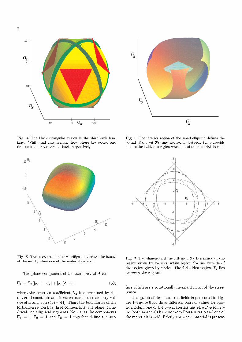
Fig. 2 The black triangular region is the third-rank lam-inate. White and gray regions show where the second and�rst-rank laminates are optimal, respectively. Both of the ma-terials have nonzero Poisson ratio.

yσ xσ

zσ

–15–10

–50

510

15

–15–10

–50

510

15

–15

–10

–5

0

5

10

15

Fig. 3 The interior region of the small ellipsoid de�nes thebound of the set F1, and the region between the ellipsoidsde�nes the forbidden region when one of the materials hasnonzero Poisson ratio.

Remark 2 The formula (52) shows the case when Poissonratio of materials is zero. This formula is modi�ed whenthe materials have an arbitrary Poisson ratio. In thiscase, the cylindrical and ellipsoidal parts are inclined onthe angle de�ned by the Poisson ration.

8

x

y

zσ

10

−10

−10

0

010

σ

σ

Fig. 4 The black triangular region is the third-rank lam-inate. White and gray regions show where the second and�rst-rank laminates are optimal, respectively.

xσyσ

zσ

–10–5

05

10

–10

–5

0

5

10

–10

0

10

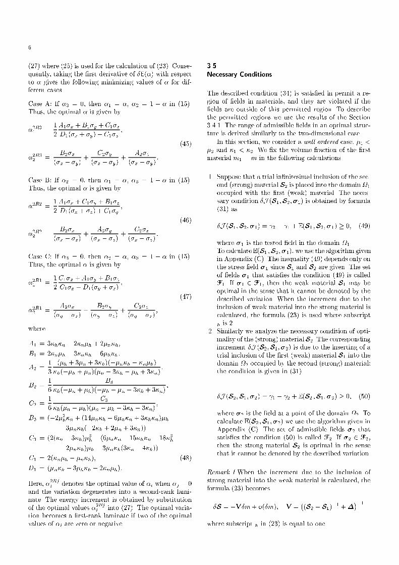
Fig. 5 The intersection of three ellipsoids de�nes the boundof the set F2 when one of the materials is void.

The plane component of the boundary of F is:

E3 = D2(j�xj+ j�y j+ j�z j)2j = 1 (53)

where the constant coe�cient D2 is determined by thematerial constants and it corresponds to stationary val-ues of � and � in (43)�(44). Thus, the boundaries of theforbidden region has three components; the plane, cylin-drical and elliptical segments. Note that the componentsE1 = 1; E2 = 1 and E3 = 1 together de�ne the sur-

σ

σ

σ

y

x

z

Fig. 6 The interior region of the small ellipsoid de�nes thebound of the set F1, and the region between the ellipsoidsde�nes the forbidden region when one of the materials is void.

xσyσ

–8

–6

–4

–2

0

2

4

6

8

–8 –6 –4 –2 2 4 6 8

Fig. 7 Two-dimensional case; Region F1 lies inside of theregion given by crosses, while region F2 lies outside ofthe region given by circles. The forbidden region Ff liesbetween the regions.

face which are a rotationally invariant norm of the stresstensor.

The graph of the permitted �elds is presented in Fig-ure 1{Figure 6 for three di�erent pairs of values for elas-tic moduli; one of the two materials has zero Poisson ra-tio, both materials have nonzero Poisson ratio and one ofthe materials is void. Brie y, the weak material is present

9

at the intersection of the three parts mentioned above,and the strong material is observed at the union of threecomponents.

Now we can formulate the underlying principle ofsti�ness optimization by a two-material structure.

4.2

Optimal Structures

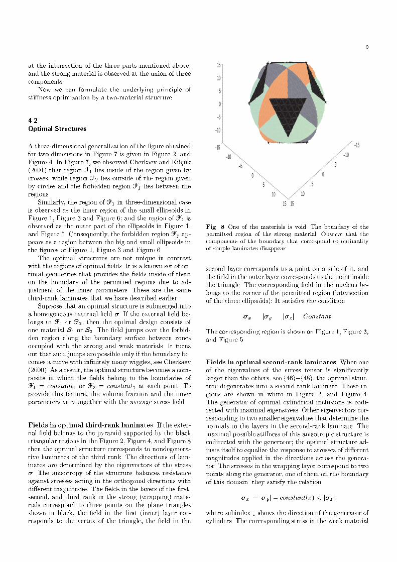
A three-dimensional generalization of the �gure obtainedfor two dimensions in Figure 7 is given in Figure 2, andFigure 4. In Figure 7, we observed Cherkaev and K�u�c�uk(2001) that region F1 lies inside of the region given bycrosses, while region F2 lies outside of the region givenby circles and the forbidden region Ff lies between theregions.

Similarly, the region of F1 in three-dimensional caseis observed as the inner region of the small ellipsoids inFigure 1, Figure 3 and Figure 6; and the region of F2 isobserved as the outer part of the ellipsoids in Figure 1,and Figure 5. Consequently, the forbidden region Ff ap-pears as a region between the big and small ellipsoids inthe �gures of Figure 1, Figure 3 and Figure 6.

The optimal structures are not unique in contrastwith the regions of optimal �elds. It is a known set of op-timal geometries that provides the �elds inside of themon the boundary of the permitted regions due to ad-justment of the inner parameters. These are the samethird-rank laminates that we have described earlier.

Suppose that an optimal structure is submerged intoa homogeneous external �eld �. If the external �eld be-longs to F1 or F2, then the optimal design consists ofone material S1 or S2. The �eld jumps over the forbid-den region along the boundary surface between zonesoccupied with the strong and weak materials. It turnsout that such jumps are possible only if the boundary be-comes a curve with in�nitely many wiggles, see Cherkaev(2000). As a result, the optimal structure becomes a com-posite in which the �elds belong to the boundaries ofF1 = constant1 or F2 = constant2 at each point. Toprovide this feature, the volume fraction and the innerparameters vary together with the average stress �eld.

Fields in optimal third-rank laminates If the exter-nal �eld belongs to the pyramid supported by the blacktriangular regions in the Figure 2, Figure 4, and Figure 8then the optimal structure corresponds to nondegenera-tive laminates of the third rank. The directions of lam-inates are determined by the eigenvectors of the stress�. The anisotropy of the structure balances resistanceagainst stresses acting in the orthogonal directions withdi�erent magnitudes. The �elds in the layers of the �rst,second, and third rank in the strong (wrapping) mate-rials correspond to three points on the plane trianglesshown in black, the �eld in the �rst (inner) layer cor-responds to the vertex of the triangle, the �eld in the

–15

–10

–5

0

5

10

15

–15

–10–5

05

10

15

–10

–5

0

5

10

15

Fig. 8 One of the materials is void. The boundary of thepermitted region of the strong material. Observe that thecomponents of the boundary that correspond to optimalityof simple laminates disappear.

second layer corresponds to a point on a side of it, andthe �eld in the outer layer corresponds to the point insidethe triangle. The corresponding �eld in the nucleus be-longs to the corner of the permitted region (intersectionof the three ellipsoids): It satis�es the condition

j�xj = j�yj = j�zj = Constant:

The corresponding region is shown on Figure 1, Figure 3,and Figure 5.

Fields in optimal second-rank laminates When oneof the eigenvalues of the stress tensor is signi�cantlylarger than the others, see (46)�(48), the optimal struc-ture degenerates into a second-rank laminate. These re-gions are shown in white in Figure 2, and Figure 4.The generator of optimal cylindrical inclusions is codi-rected with maximal eigenstress. Other eigenvectors cor-responding to two smaller eigenvalues that determine thenormals to the layers in the second-rank laminate. Themaximal possible sti�ness of this anisotropic structure iscodirected with the generator; the optimal structure ad-justs itself to equalize the response to stresses of di�erentmagnitudes applied in the directions across the genera-tor. The stresses in the wrapping layer correspond to twopoints along the generator, one of them on the boundaryof this domain. they satisfy the relation

j�xj+ j�yj = constant(x) < j�zj

where subindex z shows the direction of the generator ofcylinders. The corresponding stress in the weak material

10

Fig. 9 Permitted regions in badly-ordered case.

inside the cylinder belongs to the rib of its domain F; Itsatis�es the condition

j�xj = j�yj < j�z j:

Fields in optimal simple laminates The �elds in op-timal laminate belong to the points of elliptical surface.The �elds in both materials are constant, and they cor-respond to regular points on the elliptical components ofthe boundaries of the permitted sets.

Badly-ordered case When available materials are badly-ordered, the admissible set of stresses is restricted byelliptic hyperboloids, see Figure 9. The hyperbolic seg-ments of the boundaries replace spherical and cylindricalsegments of the boundaries for well-ordered case. In thiscase, the preferable material is de�ned not by the inten-sity of the loading, but by its type: an intensive shearloading requires the material with larger shear modulus,and an intensive bulk loading requires the other materialwith larger bulk modulus.

4.3

Topology Optimization

The asymptotic case when one of the materials is void isof special interest. The optimal design problem becomesa problem of determining of the shape of the materialframe in the design domain, or determining the numberand location of holes (voids) in a solid structure. Thisproblem is often called topology optimization problem.Our results can be easily reformulated for this case. Here

we show the results for the zero Poisson ratio materialto keep the notations simple.

De�ne the norm k�kT of the stress �eld as following:

k�kT =

� j�xj+ j�yj+ j�zj if j�xj+ j�yj � j�zj;(j�xj+ j�yj)2 + j�zj2 if j�xj+ j�yj > j�zj:

(54)

In an optimally designed body, the following conditionsare hold inside of the material:

k�kT =

8<:> C if the material is solid,= C if the material is involved in

an optimal structure.1(55)

where C is a positive constraint that depends on theamount of given material and of the intensity of externalloading, (see Figure 8).

The formulated result realizes the centuries-old ruleof rational design: the material should never be under-stressed. The material, however, may be overstressed sincewe cannot do better that place the solid material in theintensively stressed domain.

The optimal structures that realize this requirementare again non-unique, see for discussion in Cherkaev (2000).In particular, the laminate can be used as optimal struc-tures. The �rst-rank (simple) laminate is never optimalsince the structure would break apart in this asymptot-ical case. The properly adjusted second-rank laminatescorrespond to cylindrical parts of the surface in Figure 8.The third-rank laminate correspond to plane triangularregions. The volume fraction, orientation, and the geo-metric parameters of structures vary to make the �eldsin the material satisfy the conditions (55).

A

Terms Used in Section 3:4:1

In this appendix, we give explicit formulas for the termsand an algorithm used in Section 3.4.1. The terms usedin (43) and (44) is given as

B = 12(�v42 + 4v33v2 � v43 � 6v23v22 + 4v3v

32)�

3h

�36 (4v3v32 + 4v33v2 � v42 � 6v23v

22 � v43)�h�

2h (56)

�108 �6v23v22 � (v33v2 + v3v32)� 2(v42 + v43)

��2h�h:

N�1 = 2(3�h�h + �n�h + 3�n�h)�x �

(�z + �y)(6�h�h � 2�n�h + 3�n�h) (57)

N�1 = 2(3�h�h + 3�n�h + �n�h)�y �

(�x + �z)(6�h�h � 2�n�h + 3�n�h) (58)

11

D1 = �h(��h + �n)(�y + �x + �z) (59)

N�2 = ((�10�n + 18�h)�

2h � 2(�n�h + 3(�n � �h)�n)�h

� 6�n�h(�2�h + 3�n))�x � ((10�n � 6�h)�2h

+ (6�n�n � 10�n�h + 21�n�h � 18�2h)�h

� 3�n�h(�2�h + 3�n))(�y + �z); (60)

N�2 = ((12�n � 18�h)�

2h � (2�n�h � 15�n�h + 9�n�n

+ 6�2h)�h + 2�n�h(�h + 3�n))�x + 2(�h + 3�h)

(3�h + �h + 3�n)(�n � �h)�y + (18�3h

+ 6(�n � 3�n + 2�h)�2h � (9�n�n + 9�n�h

+ 10�n�h � 2�2h)�h + 2�n�h(�h + 3�n))�z ; (61)

D2 = (��n + �h)(��h + �n)((6�h � �h)�x

�(�y + �z)(3�h + �h)): (62)

N�3 = �2(��n + �h)(3�h + �h)(3�h + 3�n + �h)�x +

(18�3h � (18�n � 6�n � 12�h)�2h + (2�2h � 9�n�h

� 10�h�n � 9�n�n)�h2(3�n + �h)�n�h)�y +

((12�n � 18�h)�2h + (�9�n�n + 15�n�h

� 2�h�n � 6�2h)�h + 2(3�n + �h)�n�h)�z ; (63)

N�3 = ((2�h + 2�n)�

2h + (�9�n�h + 6�n�n � 10�n�h

+ 12�2h)�h + 3�h(�3�n�n + 2�n�h � 6�n�h

+ 6�2h))�x � 2(�h � �n)(3�h + �h)(3�h + �h

+ 3�n)�y + ((12�n � 18�h)�2h + (15�n�h � 6�2h

� 9�n�n � 2�h�n)�h + 2(�h + 3�n)�n�h)�z ; (64)

D3 = (�h � �n)(�h � �n)((3�h + �h)(�x + �y)

�(6�h � �h)�z) (65)

N�4 = �2(�h � �n)(3�h + �h)(3�h + 3�n + �h)�x

+ ((2�n � 6�h)�2h + (�2�h�n � 18�2h + 6�n�n

+ 15�n�h)�h + 3�h�n(�3�n + 4�h))�y +

((12�n � 18�h)�2h + (15�n�h � 6�2h � 9�n�n

� 2�h�n)�h + 2(�h + 3�n)�n�h)�z ; (66)

N�4 = ((18�h � 10�n)�

2h + (6�n�h � 2�n�h

� 6�n�n)�h � 6�n�h(3�n � 2�h))�y +

((18�h � 6�n)�2h + (�21�n�h + 10�n�h + 6�2h

+ 9�n�n)�h � 2�n�h(5�h + 3�n))(�x + �z); (67)

D4 = (�h � �n)(�h � �n)((3�h + �h)(�x + �z)

�(6�h � �h)�y): (68)

B

Formulas for Energies

The energy E1Ri for the �rst-rank laminate where �i = 1is de�ned as follows

E1R1 =

A�2x +B(�2y + �2z)� C(�y + �z)�x +D�y�z

18�2h(4�n + 3�n)�2h

E1R2 =

B(�2x + �2z) +A�2y � C(�x + �z)�y +D�x�z

18�2h(4�n + 3�n)�2h

E1R3 =

B(�2x + �2y) +A�2z � C(�x + �y)�z +D�x�y

18�2h(4�n + 3�n)�2h

where

A = (9(�h � �n)�n � 24�h�n + 27�2h)�2h �

�h(15�n�h � 4�h�n � 12�n�n)�h � 4�n�2h�n

B = (�9(�2n + �n�n � �n�h) + 12�h�n)�2h +

�h(4�h�n + 3�n�h � 6�n�n)�h � 4�n�2h�n

C = (3�h + 4�h)(3�h�n�h � 2�h�h�n � 3�h�n�n

+2�n�h�n)

D = (18�2n � 12�h�n + 9(�n � �h)�n)�2h +

2�h(3(�h � 2�n)�n + 4�h�n)�h � 8�n�2h�n

The energy E3Ri for the third-rank laminate where all �i'sin (15) are in the interval of (0; 1) is de�ned as follows

12

E3R1 =

(3�h + 4�h)(�y + �x + �z)2(�h � �n)

18�2h(3�n + 4�h);

E3R2 =

AA

DD

((3�h + �h)(�z + �y) + (�h � 6�h)�x)2

18�2h�2h

;

E3R3 =

AA

DD

((�6�h + �h)�z + (3�h + �h)(�x + �y))2

18�2h�2h

;

E3R4 =

AA

DD

((3�h + �h)(�x + �z) + (�h � 6�h)�y)2

18�2h�2h

;

where

DD = (�36�2h + (36�n � 24�h � 24�n)�h

+27�n�n + 21�n�h � 4�2h + 4�n�h;

AA = (3�h + 4�h)(�n � �h)(�n � �h):

C

Algorithm to Find Sets of Fields

In this section, we give an algorithm to obtain sets F1

given in (49) and F2 given in (50) for each material.Brie y, the optimal energy is calculated through the fol-lowing algorithm for any given material properties, notnecessarily restricted to well-ordered case.

E = proc(�i;Sj ;Si)

If �1; �2 and �3 2 (0; 1) E3R1

Elseif �1 = 0 then �2 = �2R11 and �3 = �2R12

If �2 2 (0; 1) then E2R11

Elseif �3 2 (0; 1) then E2R12

Elseif �2 = 0 and �3 = 1 then E1R3

Elseif �2 = 1 and �3 = 0 then E1R2

end

Elseif �1 = 1; �2 = 0 and �3 = 0 then E1R1

Elseif �2 = 0 then �1 = �2R21 and �3 = �2R22

If �1 2 (0; 1) then E2R21

Elseif �3 2 (0; 1) then E2R22

Elseif �1 = 0 and �3 = 1 then E1R3

Elseif �1 = 1 and �3 = 0 then E1R1

end

Elseif �2 = 1; �1 = 0 and �3 = 0 then E1R2

Elseif �3 = 0 then �1 = �2R31 and �2 = �2R32

If �1 2 (0; 1) then E2R31

Elseif �2 2 (0; 1) then E2R32

Elseif �1 = 0 and �2 = 1 then E1R2

Elseif �1 = 1 and �2 = 0 then E1R1

end

Elseif �3 = 1; �1 = 0 and �2 = 0 then E1R3 ;

end

The energies used in this algorithm and their notationalexplanations are given in (69) � (69).

References

Allaire, G., Bonnetier, E., Francfort, G. A., and Jouve, F.:1997, Numer. Math. 76(1), 27

Cherkaev, A. V.: 2000, Variational Methods for Structural

Optimization, Vol. 140, Springer-Verlag, New York; Berlin;Heidelberg

Cherkaev, A. V. and K�u�c�uk, I.: 2001, Structural Optimization,Submitted

13

Cherkaev, A. V. and Palais, R.: 1997, Structural Optimization

13(1), 1

Francfort, G. and Murat, F.: 1986, Arch. Rat. Mech. Anal.

94, 307

Gibiansky, L. V. and Cherkaev, A. V.: 1984, Design of Com-

posite Plates of Extremal Rigidity, Report 914, Io�e Physico-technical Institute, Acad of Sc, USSR, Leningrad, USSR, En-glish translation in Gibiansky and Cherkaev (1997a)

Gibiansky, L. V. and Cherkaev, A. V.: 1987, Microstructures

of Composites of Extremal Rigidity and Exact Estimates of

the Associated Energy Density, Report 1115, Io�e Physico-Technical Institute, Acad of Sc, USSR, Leningrad, USSR, En-glish translation in Gibiansky and Cherkaev (1997b)

Gibiansky, L. V. and Cherkaev, A. V.: 1997a, in A. V.Cherkaev and R. V. Kohn (eds.), Topics in the Mathemat-

ical Modelling of Composite Materials, Vol. 31 of Progressin nonlinear di�erential equations and their applications, pp95{137, Birkh�auser Boston, Boston, MA, Translation. Theoriginal publication in Gibiansky and Cherkaev (1984)

Gibiansky, L. V. and Cherkaev, A. V.: 1997b, in A. V.Cherkaev and R. V. Kohn (eds.), Topics in the Mathemat-

ical Modelling of Composite Materials, Vol. 31 of Progressin nonlinear di�erential equations and their applications, pp273{317, Birkh�auser Boston, Boston, MA

K�u�c�uk, I.: 2001, Ph.D. thesis, University of Utah

Lipton, R. and Diaz, A.: 1995, in N. Olho� and G. Roz-vany (eds.), Structural and Multidisciplinary Optimization,pp 161{168, Pergamon, Oxford, UK, 1995, Goslar, Germany

Lurie, K. A.: 1975, Optimal Control in Problems of Mathe-

matical Physics, Nauka, Moscow, Russia, in Russian

Lurie, K. A.: 1993, Applied Optimal Control Theory of Dis-

tributed Systems, Plenum Press, New York ,USA, New York

Olho�, N., Scheel, J., and R�nholt, E.: 1998, Structural Op-timization 16, 1