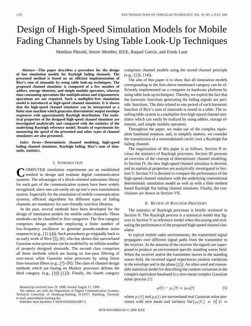
1178 IEEE TRANSACTIONS ON VEHICULAR TECHNOLOGY, VOL. 49, NO. 4, JULY 2000

Design of High-Speed Simulation Models for MobileFading Channels by Using Table Look-Up Techniques

Matthias Pätzold, Senior Member, IEEE, Raquel García, and Frank Laue

Abstract—This paper describes a procedure for the designof fast simulation models for Rayleigh fading channels. Thepresented method is based on an efficient implementation ofRice’s sum of sinusoids by using table look-up techniques. Theproposed channel simulator is composed of a few number ofadders, storage elements, and simple modulo operators, whereastime-consuming operations like multiplications and trigonometricoperations are not required. Such a multiplier-free simulationmodel is introduced as high-speed channel simulator. It is shownthat the high-speed channel simulator can be interpreted as afinite state machine which generates deterministic output envelopesequences with approximately Rayleigh distribution. The statis-tical properties of the designed high-speed channel simulator areinvestigated analytically and compared with the statistics of theunderlying Rayleigh reference model. Results of experiments formeasuring the speed of the presented and other types of channelsimulators are also presented.

Index Terms—Deterministic channel modeling, high-speedfading channel simulator, Rayleigh fading, Rice’s sum of sinu-soids, statistics.

I. INTRODUCTION

COMPUTER simulation experiments are an establishedmethod to design and evaluate digital communication

systems. The advantages of a block-oriented subroutine libraryfor each part of the communication system have been widelyrecognized, since one can easily set up one’s own transmissionsystem. Especially for the simulation of mobile communicationsystems, efficient algorithms for different types of fadingchannels are mandatory for user-friendly tool-box libraries.

In the past, several methods have been developed for thedesign of simulation models for mobile radio channels. Thesemethods can be classified in four categories. The first categorycomprises design methods employing a finite number oflow-frequency oscillators to generate pseudo-random noisesequences (e.g., [1]–[4]). Such procedures go originally back toan early work of Rice [5], [6], who has shown that narrowbandGaussian noise processes can be modeled by an infinite numberof properly designed sinusoids. The second class comprisesall those methods which are basing on low-pass filtering ofzero-mean white Gaussian noise processes by using lineartime-invariant filters (e.g., [7]–[9]). The class of channel designmethods which are basing on Markov processes defines thethird category (e.g., [10]–[12]). Finally, the fourth category

Manuscript received June 19, 1998; revised August 17, 1999.The authors are with the Department of Digital Communication Systems,

Technical University of Hamburg-Harburg, D-21071 Hamburg, Germany(e-mail: paetzold@tu-harburg.de).

Publisher Item Identifier S 0018-9545(00)03687-2.

comprises channel models using the stored channel principle(e.g., [13], [14]).

The aim of this paper is to show that all simulation modelscorresponding to the first above mentioned category can be ef-ficiently implemented on a computer or hardware platform byusing table look-up techniques. Thereby, we exploit the fact thatthe harmonic functions generating the fading signals are peri-odic functions. The data related to one period of each harmonicfunction of Rice’s sum of sinusoids is stored in a table. The re-sulting table system is a multiplier-free high-speed channel sim-ulator which can easily be realized by using adders, storage el-ements, and simple modulo operators.

Throughout the paper, we make use of the complex equiv-alent baseband notation, and, to simplify matters, we considerthe transmission of a nonmodulated carrier over a Rayleigh flatfading channel.

The organization of this paper is as follows. Section II re-views the statistics of Rayleigh processes. Section III presentsan overview of the concept of deterministic channel modeling.In Section IV, the new high-speed channel simulator is derived,and its statistical properties are analytically investigated in Sec-tion V. Section VI is devoted to compare the performance of thehigh-speed channel simulator with the underlying conventionaldeterministic simulation model as well as with a filter methodbased Rayleigh flat fading channel simulator. Finally, the con-clusions are drawn in Section VII.

II. REVIEW OF RAYLEIGH PROCESSES

The statistics of Rayleigh processes is briefly reviewed inSection II. The Rayleigh process is a statistical model that fig-ures in Section V as reference model when discussing and eval-uating the performance of the proposed high-speed channel sim-ulator.

In typical mobile radio environments, the transmitted signalpropagates over different signal paths from the transmitter tothe receiver. At the antenna of the receiver the signals are super-posed to produce an environment specific standing waves field.When the receiver and/or the transmitter moves in the standingwaves field, the received signal experiences random variationsin the envelope and in the phase [15]. An often used and reason-able statistical model for describing the random variations in thecomplex equivalent baseband is a zero-mean complex Gaussiannoise process [1]

(1)

where and are narrowband real Gaussian noise pro-cesses with zero mean and variance Var (

0018-9545/00$10.00 © 2000 IEEE

PÄTZOLD et al.: DESIGN OF HIGH-SPEED SIMULATION MODELS 1179

Fig. 1. Analytical model for Rayleigh processes.

). The Gaussian processes and are often as-sumed to be statistically independent. If that is the case, thecross-correlation function (CCF) of and is zero. Ingeneral, a real Gaussian noise process is completely describedby its mean and autocorrelation function (ACF) [16]. For an om-nidirectional receiving antenna in a two-dimensional isotropicscattering environment, it was shown in the pioneering work ofClark [17] that the ACF of can be represented by

(2)

where denotes the maximum Doppler frequency, andis the zeroth order Bessel function of the first kind. The Fouriertransform of (2) gives the Doppler power spectral density (PSD)

(3)

which is often called in literature Jakes PSD [1].A Rayleigh process, , is defined as the envelope of (1),

i.e.,

(4)

The probability density function (PDF) of is known asRayleigh density [16]

(5)

Furthermore, the corresponding cumulative distribution func-tion (CDF), defined by Prob , can be ex-pressed by [18]

(6)

The phase of defines a further random process, namely, with uniform distribution over the interval

, that is, the PDF of the phase becomes

(7)

Fig. 1 shows the structure of an analytical model for a Rayleighflat fading channel. Thereby, denotes a zero-meanwhite Gaussian noise (WGN) process with normalized vari-ance Var , and the transfer function of

each filter is adapted to the Doppler PSD (3) according to. Henceforth, we designate

channel design methods employing linear filter techniques asfilter methods.

III. OVERVIEW OF DETERMINISTIC CHANNEL MODELING

Aside from the filter method, there exists another fun-damental method for modeling narrowband Gaussian noiseprocesses: the Rice method. The principle of Rice’s method[5], [6] implies that a Gaussian noise process can bemodeled by a superposition of an infinite number of weightedharmonic functions with equidistant frequencies and randomphases according to

(8)

where the gains and discrete Doppler frequencies aregiven by

(9a)

(9b)

respectively. Thereby, the random phases are uniformlydistributed over the interval , and the quantity ischosen such that (9b) covers the whole frequency range of in-terest, where if . Equation (8) describes ananalytical model for Gaussian processes that cannot be imple-mented on a computer due to the infinite number of sinusoids.When is finite, we obtain another stochastic process

(10)

which is strictly speaking non-Gaussian distributed. But never-theless the PDF of is close to a Gaussian density ifis sufficient, say . Only in the limit , theprocess follows the ideal Gaussian distribution, and wemay write . It should be noted that is evennow a stochastic process due to the assumed random phases

. Its implementation on a computer can easily be performed

1180 IEEE TRANSACTIONS ON VEHICULAR TECHNOLOGY, VOL. 49, NO. 4, JULY 2000

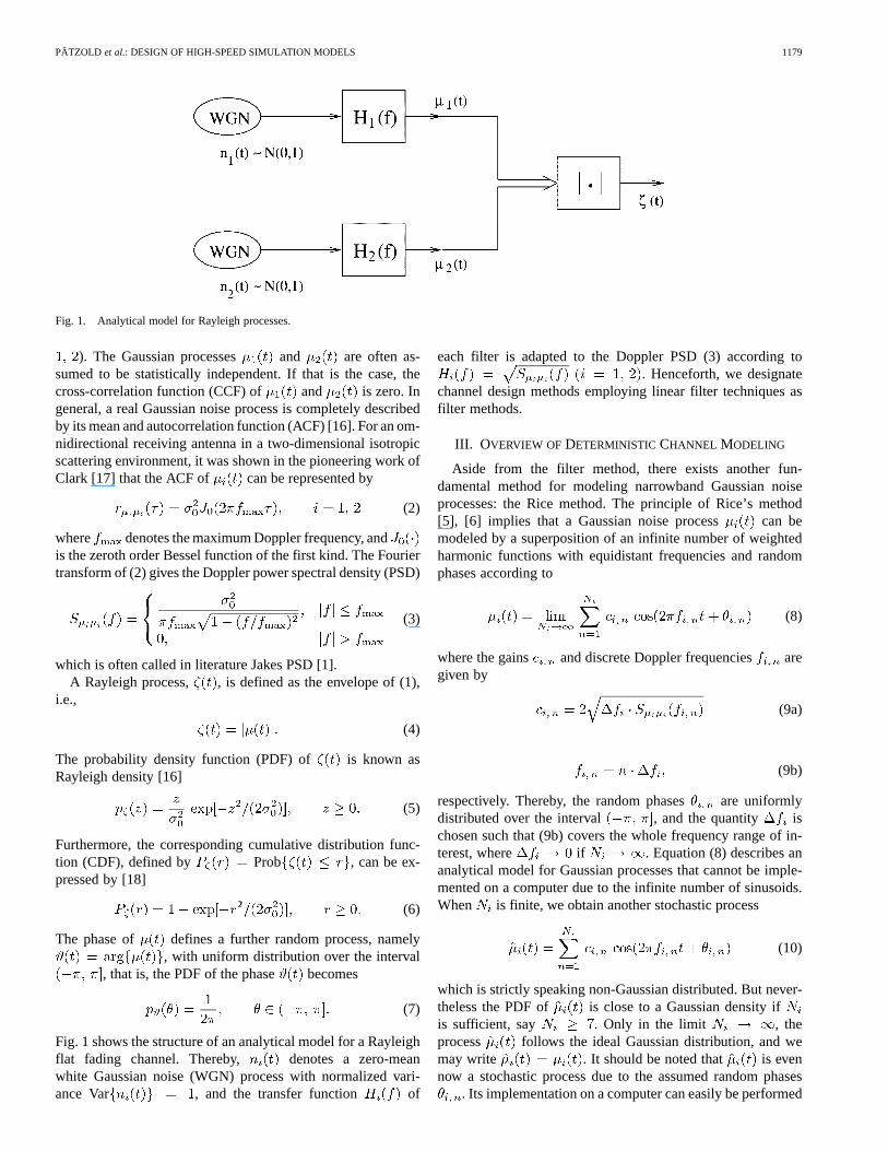
Fig. 2. Structure of deterministic Rayleigh processes (direct realization form).

and results in a stochastic simulation model. During the simu-lation, the phases and all other model parameters are keptconstant, so that is now neither more a random processbut a sample function which is per definition completely de-termined for all time . To distinguish between the stochasticprocess with random phases and the corresponding deter-ministic process (sample function), we use for the latter one thenotation

(11)

where the phases are now constant quantities, and thegains and discrete Doppler frequencies are—at themoment—furthermore given by (9a) and (9b), respectively.Let , then the deterministic process tends to asample function of the stochastic Gaussian process . Toemphasize this property, the function has been introducedin [19] asdeterministic Gaussian process. By analogy with (1)

(12)

is calledcomplex deterministic Gaussian process, and, conse-quently

(13)

represents adeterministic Rayleigh process[20]. A direct real-ization of deterministic Rayleigh processes leads to the time-continuous structure shown in Fig. 2.

The problem with (9a) and (9b) is now twofold. First, the pe-riod of is relatively small due to the equally spaced dis-crete Doppler frequencies . Second, the density ofis nonoptimal Gaussian distributed. From the central limit the-orem it follows that the density of is for a given numberof sinusoids only optimal Gaussian distributed bykeeping the power constraint if all gains are equal [19].This equal gain requirement is not fulfilled when Rice’s orig-inal method is used as can be seen immediately by substituting(3) in (9a). To overcome the problems caused by (9a) and (9b)several new methods for the computation of the model param-eters have been proposed in recent years. Forexample, the Monte Carlo method [21], [2], the method of equalareas [4], the -norm method [19], and the method of exactDoppler spread [19]. Even the in-phase and quadrature compo-nents of the well-known Jakes simulator (see [1, p. 70]) can bebrought onto the form (11) [22]. For short, we restrict our in-vestigations in the sequel to the method of exact Doppler spread(MEDS) and the Jakes method (JM).

1) Parameters by Using the MEDS [19]:Applying theMEDS to the Jakes PSD (3) gives the following closed formsolutions for the gains and discrete Doppler frequencies

(14a)

(14b)

PÄTZOLD et al.: DESIGN OF HIGH-SPEED SIMULATION MODELS 1181

for all . The phases areobtained by taking drawings from a random generatoruniformly distributed over the interval . Thereby, thenumber of sinusoids and are in general related by

what guarantees the design of zero cross-corre-lated deterministic Gaussian processes and .

Parameters by Using the JM [1]:When the JM is used, thegains , discrete Doppler frequencies , and phasescan be expressed in closed form as follows [22]:

,

,

(15a)

,

(15b)

(15c)

where . According to the JM, the discreteDoppler frequencies and are identical for all

, and, thus, the processes andare correlated.

Of further interest are some basic statistical properties of de-terministic processes like the ACF, PSD, CCF, PDF, and CDF.The statistics of deterministic processes has been investigatedin detail in [19]. Here, we only present some basic results as faras they are of importance for the understanding of the rest of thepaper.

A. ACF, PSD, and CCF

The ACF and the corresponding Doppler PSDof the deterministic Gaussian process may be

represented by [19]

(16a)

(16b)

respectively. For the MEDS, one can show by putting (14a) and(14b) in (16a) that tends to if .This is in contrast to the JM, where the inequality

holds even if , as can be proved by substi-tuting (15a) and (15b) in (16a). The CCF of the deter-ministic Gaussian processes and is given by [19]

ifif

(17)

for all and , whereindicates the minimum value of and , i.e.,

. For the MEDS it can easily be guaranteedthat the designed processes and are uncorrelated,i.e., , e.g., by defining . Forthe JM, where is per definition equal to , we obtain

.

B. PDF and CDF

General analytical expressions for the density of the envelopeand phase of complex determin-

istic Gaussian processes have been de-rived in [19]. There the following results are presented:

(18a)

(18b)where

(19)

denotes the PDF of the deterministic Gaussian processasintroduced by (11). Note that , and thus andare only functions of the gains and the number of sinusoids

. From the central limit theorem it follows for both methods(MEDS and JM) that (19) tends in the limit to aGaussian density with zero mean and variance. Hence, when

then it follows immediately from the expressions(18a) and (18b) that approaches the Rayleigh density (5),whereas approaches the uniform density (7). However, forfinite values of , we may write and

, thereby it is worth mentioning that the approximationsare better for the MEDS than for the JM.

After performing some algebraic manipulations, we can ob-tain from (18a) the following CDF Prob of

:

(20)

1182 IEEE TRANSACTIONS ON VEHICULAR TECHNOLOGY, VOL. 49, NO. 4, JULY 2000

Fig. 3. Structure of the high-speed channel simulator.

Thus, the above result enables an analytical investigation of theCDF of deterministic Rayleigh processes . It should be clearthat we may write if .

IV. DESIGN OFHIGH-SPEEDCHANNEL SIMULATORS

An efficient implementation of the conventional deterministicmodel described in Section III can be achieved by applying tablelook-up techniques. Each sinusoidal function in (11) issubstituted by a table which stores the data related to one periodof . For the resulting discrete-time simulation model, anaddress generator is required to have access to the registers ofthe tables. The outputs of each block of tables are addedin order to obtain an equivalent discrete-time realization of thedeterministic Gaussian processes ( ). Fig. 3 showsthe discrete-time structure of the resulting tables system.

The equivalent discrete-time realization of the deterministicGaussian processes is called discrete deterministicGaussian process which can be expressed by

(21)

where denotes the sampling interval. Obviously, the discretedeterministic Gaussian process is obtained by samplingthe continuous-time deterministic Gaussian process at

, whereby additionally the discrete Dopplerfrequencies and phases are replaced by and ,respectively. It will be shown below that the new parameters

and are slightly modified versions of the original pa-rameters and , in the order mentioned.

In general, a Rayleigh process is obtained by taking theabsolute value of a complex Gaussian noise process. Accordingto our method, we can approximately model the statistics ofa sample function of a Rayleigh process by combining tworeal table blocks to a so-calleddiscrete complex deterministicGaussian process

(22)

and then taking at each instantthe absolute value according to

(23)

where is nameddiscrete deterministic Rayleigh process.The table that corresponds to the sinusoidal function

is referred in Fig. 3 as Tab . The number of entries of the tableTab corresponds to the table length which will be denoted as

. To find an expression for the table length , recall thatit is sufficient to store only one period of the underlying sinu-soidal function . Thereby, we have to take into account

PÄTZOLD et al.: DESIGN OF HIGH-SPEED SIMULATION MODELS 1183

Fig. 4. Evaluation of the relative error" according to (26) forf = 91

Hz as function of the sampling intervalT .

the influence of the sampling interval . In order to obtain forany given sampling interval an integer number for the tablelength , the discrete Doppler frequency of the originalsinusoid has to be slightly modified according to

round(24)

where is the sampling frequency, and the operation rounddenotes the nearest integer to. The period of the resulting dis-crete-time sinusoid corresponds to the table lengthwhich is now given by

round (25)

By selecting a sufficiently large value for the sampling fre-quency , the modified discrete Doppler frequency

is very close to the original quantity . The quality ofthe approximation and, consequently, of the statis-tics of the resulting discrete-time simulation model, depends onthe sampling frequency . A measure for the approximationerror is the relative error of , i.e.,

(26)

The behavior of is shown in Fig. 4 over the sampling in-terval for a discrete Doppler frequency of 91 Hz. Thepresented result shows us that the relative error is less than

5% if the sampling interval is less than . Note thatit follows from (24) that we may write if

.The complexity of the tables system is closely related with

the tables lengths . From (25), we realize that is pro-portional to the sampling frequency. Hence, a compromisebetween the precision and the complexity of the tables systemmust be found by choosing an adequate value for. Experi-mental results have revealed that an adequate value for the sam-pling frequency is given if is within the range of

.

Since the number of samples of the discrete sinusoidstored in the table Tab is , then the phase can onlytake values from a discrete set of equidistant phases withinthe interval , i.e.,

(27)whereby each of these values corresponds to a specific initialposition in the table Tab . The phases are chosen fromthe above set in such a way that is nearest to .Hence, it follows for that we may write .

From the fact that and are tending to and ,respectively, if approaches to zero, it follows:if . Moreover, by taking the results of Section III intoaccount, we can say that tends to a sample function of theGaussian process if and .

A. Tables System

The tables system is composed of tables, wherebyeach one is equivalent to a sinusoidal function in the con-ventional deterministic model. The data stored in the tablescontain the full information to compute the correspondingdiscrete deterministic Gaussian process at any instant

.The entry of the table Tab at position

corresponds to the value of thediscrete-time sinusoidal function at instant , i.e.,

(28)

where and . If the entries of thetable Tab are sequentially read from the beginning, then thetable output sequence is , , , ,

, , and, therefore, the discrete-time si-nusoid can completely be reconstructed for all

.The address generator (AG) shown in Fig. 3 is required to

enable the access to the data stored in the tables. The number ofaddresses that the AG generates is , i.e., one addressfor each table. Let us denote the address of the table Tabatinstant by , then the way of operation of the AG caneasily be described as follows. At instant, the AG points to acertain register in the table at position . At the nextinstant , the generated address corresponds to the positionof the next lower register in the table shown in Fig. 3. When thelast position of the table is reached, then the AG points at thenext instant to the first register again.

Let us start from the initial addresses which are deter-mined by the phases , then we can compute recursively theaddresses at each instant by using

(29)

for all , where the notationdenotes the modulo operation. It should be mentioned that themodulo operation has been introduced here only for mathemat-ical convenience. Its implementation on a computer can easilybe achieved by using an adder and an operation.

1184 IEEE TRANSACTIONS ON VEHICULAR TECHNOLOGY, VOL. 49, NO. 4, JULY 2000

B. Matrix System

The new implementation form of the conventional determin-istic model can also be interpreted as a matrix system. There-fore, we define a matrix for the block of tables which de-termine the discrete deterministic Gaussian process

. The number of rows of the matrix is equal to thenumber of tables . Thereby, the th row of contains thedata of the table Tab . Hence, the length of the largest tabledefines the number of columns of , i.e.,

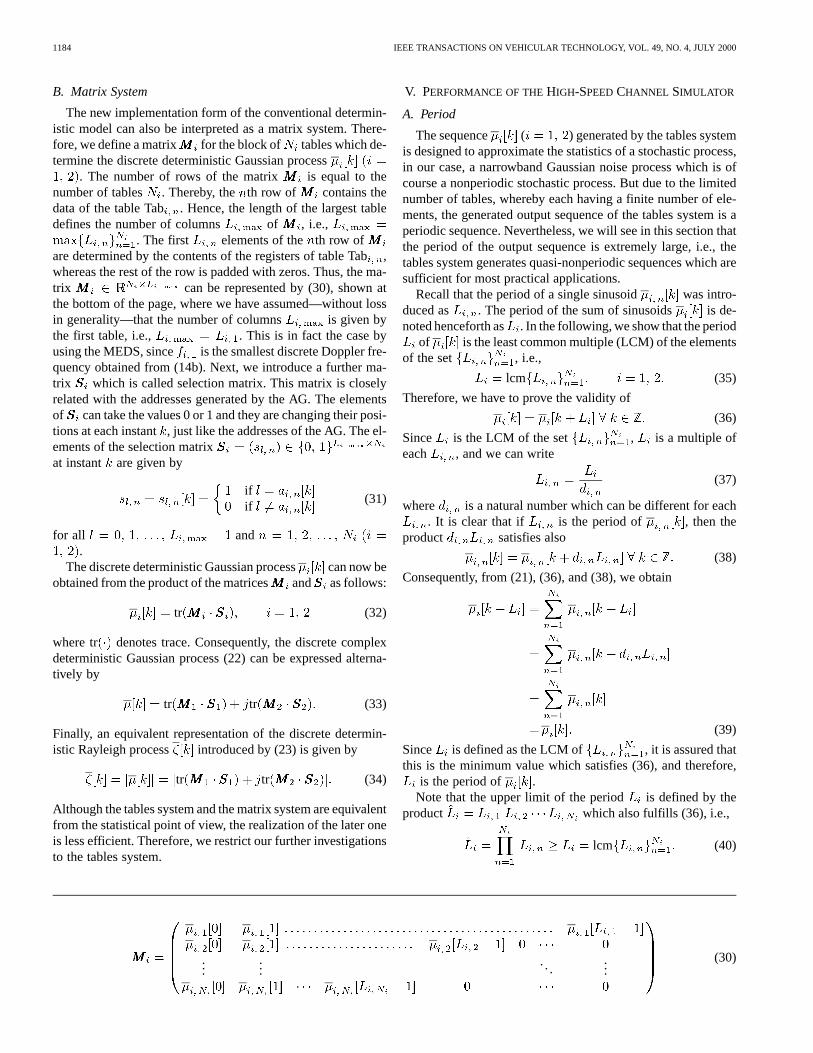
. The first elements of the th row ofare determined by the contents of the registers of table Tab,whereas the rest of the row is padded with zeros. Thus, the ma-trix can be represented by (30), shown atthe bottom of the page, where we have assumed—without lossin generality—that the number of columns is given bythe first table, i.e., . This is in fact the case byusing the MEDS, since is the smallest discrete Doppler fre-quency obtained from (14b). Next, we introduce a further ma-trix which is called selection matrix. This matrix is closelyrelated with the addresses generated by the AG. The elementsof can take the values 0 or 1 and they are changing their posi-tions at each instant, just like the addresses of the AG. The el-ements of the selection matrixat instant are given by

ifif

(31)

for all and.

The discrete deterministic Gaussian process can now beobtained from the product of the matrices and as follows:

tr (32)

where tr denotes trace. Consequently, the discrete complexdeterministic Gaussian process (22) can be expressed alterna-tively by

tr tr (33)

Finally, an equivalent representation of the discrete determin-istic Rayleigh process introduced by (23) is given by

tr tr (34)

Although the tables system and the matrix system are equivalentfrom the statistical point of view, the realization of the later oneis less efficient. Therefore, we restrict our further investigationsto the tables system.

V. PERFORMANCE OF THEHIGH-SPEEDCHANNEL SIMULATOR

A. Period

The sequence ( ) generated by the tables systemis designed to approximate the statistics of a stochastic process,in our case, a narrowband Gaussian noise process which is ofcourse a nonperiodic stochastic process. But due to the limitednumber of tables, whereby each having a finite number of ele-ments, the generated output sequence of the tables system is aperiodic sequence. Nevertheless, we will see in this section thatthe period of the output sequence is extremely large, i.e., thetables system generates quasi-nonperiodic sequences which aresufficient for most practical applications.

Recall that the period of a single sinusoid was intro-duced as . The period of the sum of sinusoids is de-noted henceforth as . In the following, we show that the period

of is the least common multiple (LCM) of the elementsof the set , i.e.,

lcm (35)

Therefore, we have to prove the validity of

(36)

Since is the LCM of the set , is a multiple ofeach , and we can write

(37)

where is a natural number which can be different for each. It is clear that if is the period of , then the

product satisfies also

(38)

Consequently, from (21), (36), and (38), we obtain

(39)

Since is defined as the LCM of , it is assured thatthis is the minimum value which satisfies (36), and therefore,

is the period of .Note that the upper limit of the period is defined by the

product which also fulfills (36), i.e.,

lcm (40)

......

. . ....

(30)

PÄTZOLD et al.: DESIGN OF HIGH-SPEED SIMULATION MODELS 1185

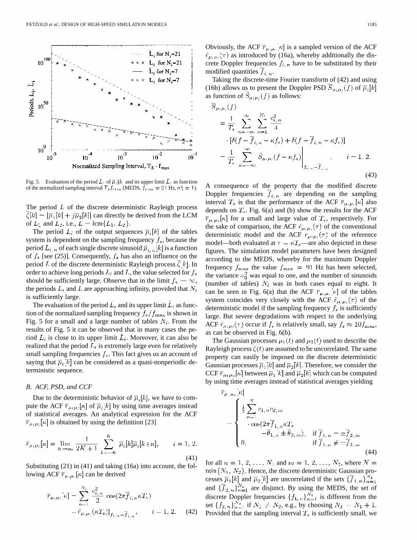
Fig. 5. Evaluation of the periodL of � [k] and its upper limit̂L as functionof the normalized sampling intervalT f (MEDS,f = 91 Hz,� = 1).

The period of the discrete deterministic Rayleigh processcan directly be derived from the LCM

of and , i.e., lcm .The period of the output sequences of the tables

system is dependent on the sampling frequency, because theperiod of each single discrete sinusoid is a functionof [see (25)]. Consequently, has also an influence on theperiod of the discrete deterministic Rayleigh process . Inorder to achieve long periods and , the value selected forshould be sufficiently large. Observe that in the limit ,the periods and are approaching infinity, provided thatis sufficiently large.

The evaluation of the period and its upper limit as func-tion of the normalized sampling frequency is shown inFig. 5 for a small and a large number of tables. From theresults of Fig. 5 it can be observed that in many cases the pe-riod is close to its upper limit . Moreover, it can also berealized that the period is extremely large even for relativelysmall sampling frequencies. This fact gives us an account ofsaying that can be considered as a quasi-nonperiodic de-terministic sequence.

B. ACF, PSD, and CCF

Due to the deterministic behavior of , we have to com-pute the ACF of by using time averages insteadof statistical averages. An analytical expression for the ACF

is obtained by using the definition [23]

(41)Substituting (21) in (41) and taking (16a) into account, the fol-lowing ACF can be derived

(42)

Obviously, the ACF is a sampled version of the ACFas introduced by (16a), whereby additionally the dis-

crete Doppler frequencies have to be substituted by theirmodified quantities .

Taking the discrete-time Fourier transform of (42) and using(16b) allows us to present the Doppler PSD ofas function of as follows:

(43)

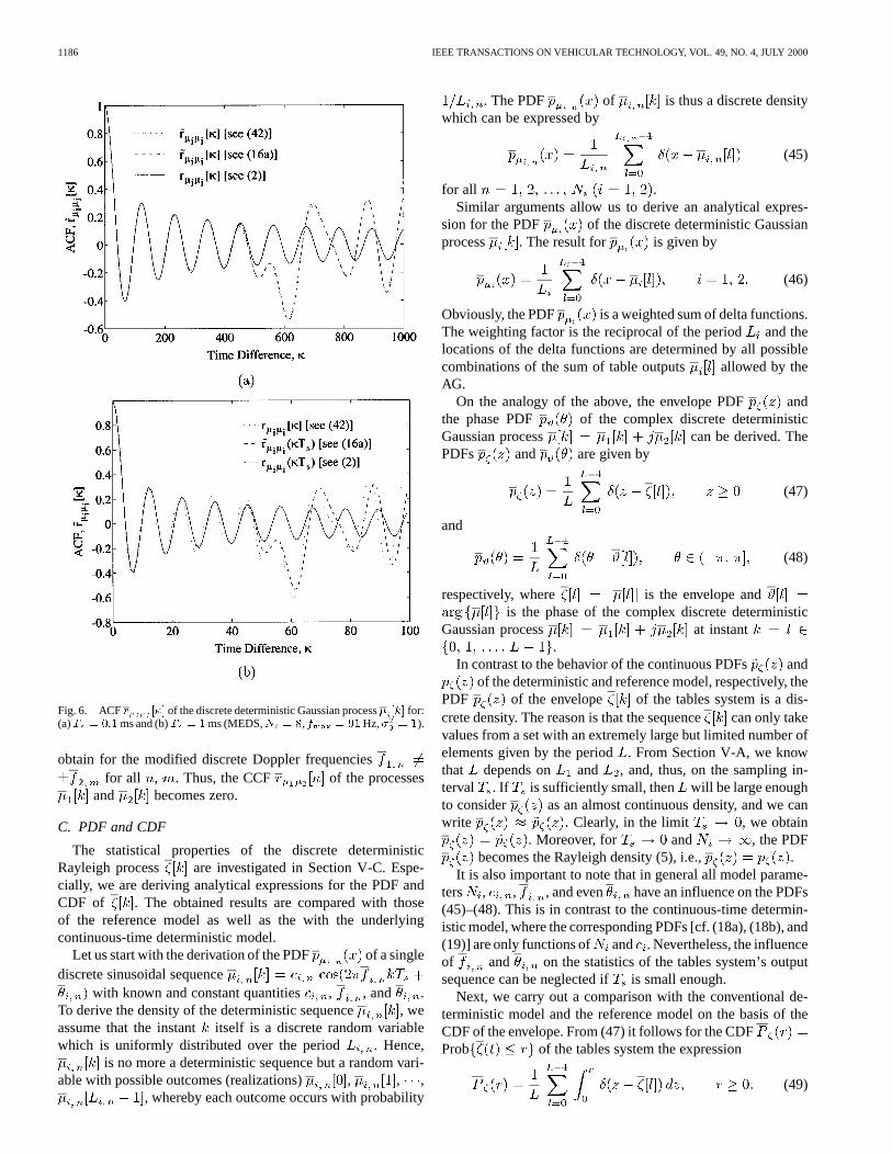
A consequence of the property that the modified discreteDoppler frequencies are depending on the samplinginterval is that the performance of the ACF alsodepends on . Fig. 6(a) and (b) show the results for the ACF

for a small and large value of , respectively. Forthe sake of comparison, the ACF of the conventionaldeterministic model and the ACF of the referencemodel—both evaluated at —are also depicted in thesefigures. The simulation model parameters have been designedaccording to the MEDS, whereby for the maximum Dopplerfrequency the value Hz has been selected,the variance was equal to one, and the number of sinusoids(number of tables) was in both cases equal to eight. Itcan be seen in Fig. 6(a) that the ACF of the tablessystem coincides very closely with the ACF of thedeterministic model if the sampling frequencyis sufficientlylarge. But severe degradations with respect to the underlyingACF occur if is relatively small, say ,as can be observed in Fig. 6(b).

The Gaussian processes and used to describe theRayleigh process are assumed to be uncorrelated. The sameproperty can easily be imposed on the discrete deterministicGaussian processes and . Therefore, we consider theCCF between and which can be computedby using time averages instead of statistical averages yielding

ifif

(44)

for all and , where. Hence, the discrete deterministic Gaussian pro-

cesses and are uncorrelated if the setsand are disjunct. By using the MEDS, the set ofdiscrete Doppler frequencies is different from theset if , e.g., by choosing .Provided that the sampling interval is sufficiently small, we

1186 IEEE TRANSACTIONS ON VEHICULAR TECHNOLOGY, VOL. 49, NO. 4, JULY 2000

Fig. 6. ACFr [�] of the discrete deterministic Gaussian process� [k] for:(a)T = 0:1ms and (b)T = 1ms (MEDS,N = 8,f = 91Hz,� = 1).

obtain for the modified discrete Doppler frequenciesfor all , . Thus, the CCF of the processes

and becomes zero.

C. PDF and CDF

The statistical properties of the discrete deterministicRayleigh process are investigated in Section V-C. Espe-cially, we are deriving analytical expressions for the PDF andCDF of . The obtained results are compared with thoseof the reference model as well as the with the underlyingcontinuous-time deterministic model.

Let us start with the derivation of the PDF of a singlediscrete sinusoidal sequence

with known and constant quantities , , and .To derive the density of the deterministic sequence , weassume that the instant itself is a discrete random variablewhich is uniformly distributed over the period . Hence,

is no more a deterministic sequence but a random vari-able with possible outcomes (realizations) , , ,

, whereby each outcome occurs with probability

. The PDF of is thus a discrete densitywhich can be expressed by

(45)

for all .Similar arguments allow us to derive an analytical expres-

sion for the PDF of the discrete deterministic Gaussianprocess . The result for is given by

(46)

Obviously, the PDF is a weighted sum of delta functions.The weighting factor is the reciprocal of the periodand thelocations of the delta functions are determined by all possiblecombinations of the sum of table outputs allowed by theAG.

On the analogy of the above, the envelope PDF andthe phase PDF of the complex discrete deterministicGaussian process can be derived. ThePDFs and are given by

(47)

and

(48)

respectively, where is the envelope andis the phase of the complex discrete deterministic

Gaussian process at instant.

In contrast to the behavior of the continuous PDFs andof the deterministic and reference model, respectively, the

PDF of the envelope of the tables system is a dis-crete density. The reason is that the sequencecan only takevalues from a set with an extremely large but limited number ofelements given by the period. From Section V-A, we knowthat depends on and , and, thus, on the sampling in-terval . If is sufficiently small, then will be large enoughto consider as an almost continuous density, and we canwrite Clearly, in the limit , we obtain

. Moreover, for and , the PDFbecomes the Rayleigh density (5), i.e., .

It is also important to note that in general all model parame-ters , , , and even have an influence on the PDFs(45)–(48). This is in contrast to the continuous-time determin-istic model, where the corresponding PDFs [cf. (18a), (18b), and(19)] are only functions of and . Nevertheless, the influenceof and on the statistics of the tables system’s outputsequence can be neglected if is small enough.

Next, we carry out a comparison with the conventional de-terministic model and the reference model on the basis of theCDF of the envelope. From (47) it follows for the CDFProb of the tables system the expression

(49)

PÄTZOLD et al.: DESIGN OF HIGH-SPEED SIMULATION MODELS 1187

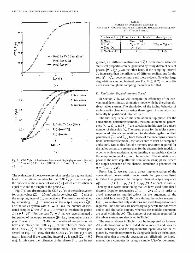
Fig. 7. CDFP (r) of the discrete deterministic Rayleigh process�[k] for: (a)T = 0:5 ms and (b)T = 5 ms (MEDS,N = 7, N = 8, f = 91 Hz,� = 1).

The evaluation of the above expression results for a given signallevel in a rational number for the CDF that is simplythe quotient of the number of values which are less than orequal to and the length of the period.

Fig. 7(a) and (b) presents the CDF of the tables systemfor small values ( ms) and large values ( ms) ofthe sampling interval , respectively. The results are obtainedby simulating samples of the output sequence .For the tables system with ms, the number of eval-uated samples was which is less than the period

. For the case ms, we have simulated afull period of the output sequence , i.e., the number of sam-ples was . For the sake of comparison, wehave also plotted the CDF of the reference model andthe CDFs of the deterministic model. The results pre-sented in Fig. 7(a) show that the CDFs and arenearly identical if the sampling interval is small (ms). In this case, the influence of the phases can be ne-

TABLE INUMBER OF OPERATIONS REQUIRED TO

COMPUTE ~�[k] (CONVENTIONAL DETERMINISTIC SIMULATION MODEL) AND

�[k] (TABLES SYSTEM)

glected, i.e., different realizations of with almost identicalstatistical properties can be generated by using different sets ofphases . On the other hand, if the sampling interval

increases, then the influence of different realizations for thesets becomes more and more evident. Note that largedegradations can be obtained [see Fig. 7(b)] ifis nonsuffi-cient even though the sampling theorem is fulfilled.

D. Realization Expenditure and Speed

In Section V-D, we will compare the efficiency of the con-ventional deterministic simulation model with the therefrom de-rived tables system. The simulation of the fading behavior ofmobile radio channels by using these types of simulators canbasically be partitioned into two steps.

The first step is called the simulation set-up phase. For theconventional deterministic model, the simulation model param-eters ( , , and ) are calculated in this step for a givennumber of sinusoids . The set-up phase for the tables systemrequires additional computations. Besides deriving the modifiedparameters and from those of the underlying conven-tional deterministic model, the tables entries must be computedand stored. Due to this fact, the memory resources required forthe tables system are greater than for the deterministic model. Inorder to achieve moderate tables lengths, a reasonable value forthe sampling interval has to be selected. The simulation runphase is the next step after the simulation set-up phase, wherethe output sequence of the channel simulator is generated for

.From Fig. 2, we see that a direct implementation of the

conventional deterministic model needs the operations listedin Table I to generate the complex channel output sequence

at each instant .Thereby, it is worth mentioning that we have used normalizeddiscrete Doppler frequencies in order toavoid unnecessary multiplications in the argument of thesinusoidal functions (11). By considering the tables system inFig. 3, we realize that only additions and modulo operations arerequired. The additions are necessary to generate the addressesand to add the table outputs, whereas the modulo operationsare used within the AG. The number of operations required forthe tables system are also listed in Table I.

The results shown in Table I can be interpreted as follows.All multiplications can be avoided, the number of additions re-main unchanged, and the trigonometric operations can be re-placed by modulo operations by using table look-up techniques.Remember that a modulo operation can efficiently be imple-mented on a computer by using a simple command.

1188 IEEE TRANSACTIONS ON VEHICULAR TECHNOLOGY, VOL. 49, NO. 4, JULY 2000

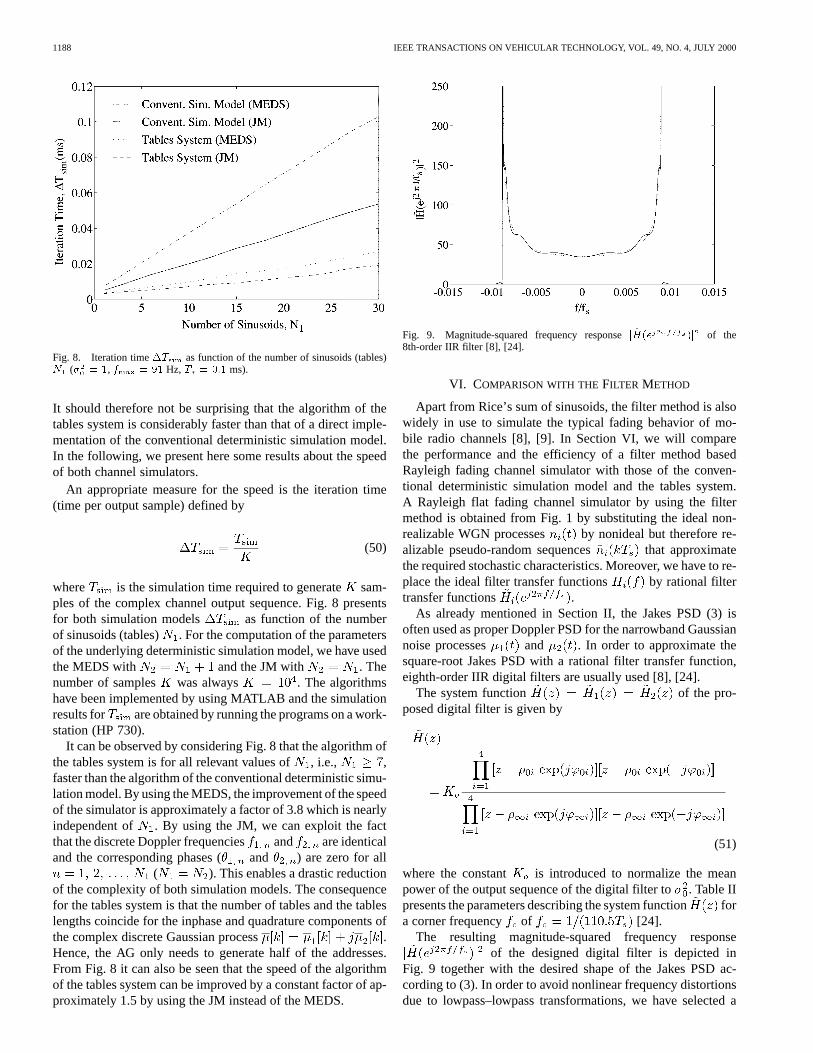
Fig. 8. Iteration time�T as function of the number of sinusoids (tables)N (� = 1, f = 91 Hz, T = 0:1 ms).

It should therefore not be surprising that the algorithm of thetables system is considerably faster than that of a direct imple-mentation of the conventional deterministic simulation model.In the following, we present here some results about the speedof both channel simulators.

An appropriate measure for the speed is the iteration time(time per output sample) defined by

(50)

where is the simulation time required to generatesam-ples of the complex channel output sequence. Fig. 8 presentsfor both simulation models as function of the numberof sinusoids (tables) . For the computation of the parametersof the underlying deterministic simulation model, we have usedthe MEDS with and the JM with . Thenumber of samples was always . The algorithmshave been implemented by using MATLAB and the simulationresults for are obtained by running the programs on a work-station (HP 730).

It can be observed by considering Fig. 8 that the algorithm ofthe tables system is for all relevant values of, i.e., ,faster than the algorithm of the conventional deterministic simu-lation model. By using the MEDS, the improvement of the speedof the simulator is approximately a factor of 3.8 which is nearlyindependent of . By using the JM, we can exploit the factthat the discrete Doppler frequencies and are identicaland the corresponding phases ( and ) are zero for all

( ). This enables a drastic reductionof the complexity of both simulation models. The consequencefor the tables system is that the number of tables and the tableslengths coincide for the inphase and quadrature components ofthe complex discrete Gaussian process .Hence, the AG only needs to generate half of the addresses.From Fig. 8 it can also be seen that the speed of the algorithmof the tables system can be improved by a constant factor of ap-proximately 1.5 by using the JM instead of the MEDS.

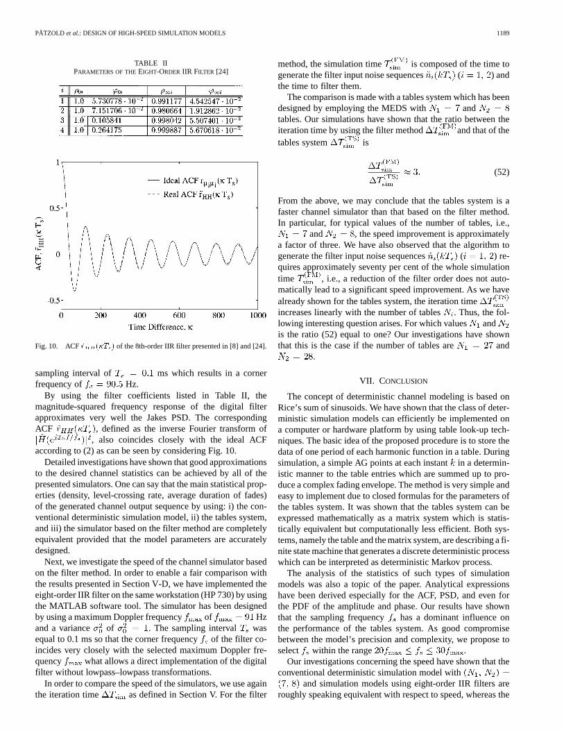
Fig. 9. Magnitude-squared frequency responsej ~H(e )j of the8th-order IIR filter [8], [24].

VI. COMPARISON WITH THEFILTER METHOD

Apart from Rice’s sum of sinusoids, the filter method is alsowidely in use to simulate the typical fading behavior of mo-bile radio channels [8], [9]. In Section VI, we will comparethe performance and the efficiency of a filter method basedRayleigh fading channel simulator with those of the conven-tional deterministic simulation model and the tables system.A Rayleigh flat fading channel simulator by using the filtermethod is obtained from Fig. 1 by substituting the ideal non-realizable WGN processes by nonideal but therefore re-alizable pseudo-random sequences that approximatethe required stochastic characteristics. Moreover, we have to re-place the ideal filter transfer functions by rational filtertransfer functions .

As already mentioned in Section II, the Jakes PSD (3) isoften used as proper Doppler PSD for the narrowband Gaussiannoise processes and . In order to approximate thesquare-root Jakes PSD with a rational filter transfer function,eighth-order IIR digital filters are usually used [8], [24].

The system function of the pro-posed digital filter is given by

(51)

where the constant is introduced to normalize the meanpower of the output sequence of the digital filter to. Table IIpresents the parameters describing the system functionfora corner frequency of [24].

The resulting magnitude-squared frequency responseof the designed digital filter is depicted in

Fig. 9 together with the desired shape of the Jakes PSD ac-cording to (3). In order to avoid nonlinear frequency distortionsdue to lowpass–lowpass transformations, we have selected a

PÄTZOLD et al.: DESIGN OF HIGH-SPEED SIMULATION MODELS 1189

TABLE IIPARAMETERS OF THEEIGHT-ORDER IIR FILTER [24]

Fig. 10. ACF~r (�T ) of the 8th-order IIR filter presented in [8] and [24].

sampling interval of ms which results in a cornerfrequency of Hz.

By using the filter coefficients listed in Table II, themagnitude-squared frequency response of the digital filterapproximates very well the Jakes PSD. The correspondingACF , defined as the inverse Fourier transform of

, also coincides closely with the ideal ACFaccording to (2) as can be seen by considering Fig. 10.

Detailed investigations have shown that good approximationsto the desired channel statistics can be achieved by all of thepresented simulators. One can say that the main statistical prop-erties (density, level-crossing rate, average duration of fades)of the generated channel output sequence by using: i) the con-ventional deterministic simulation model, ii) the tables system,and iii) the simulator based on the filter method are completelyequivalent provided that the model parameters are accuratelydesigned.

Next, we investigate the speed of the channel simulator basedon the filter method. In order to enable a fair comparison withthe results presented in Section V-D, we have implemented theeight-order IIR filter on the same workstation (HP 730) by usingthe MATLAB software tool. The simulator has been designedby using a maximum Doppler frequency of Hzand a variance of . The sampling interval wasequal to 0.1 ms so that the corner frequencyof the filter co-incides very closely with the selected maximum Doppler fre-quency what allows a direct implementation of the digitalfilter without lowpass–lowpass transformations.

In order to compare the speed of the simulators, we use againthe iteration time as defined in Section V. For the filter

method, the simulation time is composed of the time togenerate the filter input noise sequences ( ) andthe time to filter them.

The comparison is made with a tables system which has beendesigned by employing the MEDS with andtables. Our simulations have shown that the ratio between theiteration time by using the filter method and that of thetables system is

(52)

From the above, we may conclude that the tables system is afaster channel simulator than that based on the filter method.In particular, for typical values of the number of tables, i.e.,

and , the speed improvement is approximatelya factor of three. We have also observed that the algorithm togenerate the filter input noise sequences ( ) re-quires approximately seventy per cent of the whole simulationtime , i.e., a reduction of the filter order does not auto-matically lead to a significant speed improvement. As we havealready shown for the tables system, the iteration timeincreases linearly with the number of tables. Thus, the fol-lowing interesting question arises. For which valuesandis the ratio (52) equal to one? Our investigations have shownthat this is the case if the number of tables are and

.

VII. CONCLUSION

The concept of deterministic channel modeling is based onRice’s sum of sinusoids. We have shown that the class of deter-ministic simulation models can efficiently be implemented ona computer or hardware platform by using table look-up tech-niques. The basic idea of the proposed procedure is to store thedata of one period of each harmonic function in a table. Duringsimulation, a simple AG points at each instantin a determin-istic manner to the table entries which are summed up to pro-duce a complex fading envelope. The method is very simple andeasy to implement due to closed formulas for the parameters ofthe tables system. It was shown that the tables system can beexpressed mathematically as a matrix system which is statis-tically equivalent but computationally less efficient. Both sys-tems, namely the table and the matrix system, are describing a fi-nite state machine that generates a discrete deterministic processwhich can be interpreted as deterministic Markov process.

The analysis of the statistics of such types of simulationmodels was also a topic of the paper. Analytical expressionshave been derived especially for the ACF, PSD, and even forthe PDF of the amplitude and phase. Our results have shownthat the sampling frequency has a dominant influence onthe performance of the tables system. As good compromisebetween the model’s precision and complexity, we propose toselect within the range .

Our investigations concerning the speed have shown that theconventional deterministic simulation model with

and simulation models using eight-order IIR filters areroughly speaking equivalent with respect to speed, whereas the

1190 IEEE TRANSACTIONS ON VEHICULAR TECHNOLOGY, VOL. 49, NO. 4, JULY 2000

tables system is approximately three times faster, what legiti-mates us to designate the tables system as high-speed channelsimulator.

REFERENCES

[1] W. C. Jakes, Ed.,Microwave Mobile Communications. Piscataway,NJ: IEEE Press, 1993.

[2] P. Höher, “A statistical discrete-time model for the WSSUS multipathchannel,”IEEE Trans. Veh. Technol., vol. 41, pp. 461–468, Nov. 1992.

[3] P. M. Crespo and J. Jiménez, “Computer simulation of radio channelsusing a harmonic decomposition technique,”IEEE Trans. Veh. Technol.,vol. 44, pp. 414–419, Aug. 1995.

[4] M. Pätzold, U. Killat, and F. Laue, “A deterministic digital simulationmodel for Suzuki processes with application to a shadowed Rayleighland mobile radio channel,”IEEE Trans. Veh. Technol., vol. 45, pp.318–331, May 1996.

[5] S. O. Rice, “Mathematical analysis of random noise,”Bell Syst. Tech. J.,vol. 23, pp. 282–332, Jul. 1944.

[6] , “Mathematical analysis of random noise,”Bell Syst. Tech. J., vol.24, pp. 46–156, Jan. 1945.

[7] E. Lutz and E. Plöchinger, “Generating Rice processes with given spec-tral properties,”IEEE Trans. Veh. Technol., vol. VT-34, pp. 178–181,Nov. 1985.

[8] H. Brehm, W. Stammler, and M. Werner, “Design of a highly flexibledigital simulator for narrowband fading channels,” inSignal ProcessingIII: Theories and Applications. Amsterdam, The Netherlands: Else-vier Science Publishers (North-Holland), EURASIP, Sep. 1986, pp.1113–1116.

[9] S. A. Fechtel, “A novel approach to modeling and efficient simulationof frequency-selective fading radio channels,”IEEE J. Select. AreasCommun., vol. 11, pp. 422–431, Apr. 1993.

[10] F. Swarts and H. C. Ferreira, “Markov characterization of channels withsoft decision outputs,”IEEE Trans. Commun., vol. 41, pp. 678–682,May 1993.

[11] H. S. Wang and N. Moayeri, “Finite-state Markov channel—A usefulmodel for radio communication channels,”IEEE Trans. Veh. Technol.,vol. 44, pp. 163–171, Feb. 1995.

[12] W. Turin and R. Nobelen, “Hidden Markov modeling of fading chan-nels,” inProc. IEEE 48th Veh. Technol. Conf., Ottawa, ON, Canada, May1998, pp. 1234–1238.

[13] J. Hagenauer and W. Papke, “The stored channel—A simulation methodfor fading channels (in German),”FREQUENZ, vol. 36, pp. 122–129,April/May 1982.

[14] , “Data transmission for maritime and land mobiles using storedchannel simulation,” inProc. IEEE 32nd Veh. Technol. Conf., San Diego,CA, 1982, pp. 379–383.

[15] Y. Akaiwa,Introduction to Digital Mobile Communication. New York:Wiley, 1997.

[16] A. Papoulis,Probability, Random Variables, and Stochastic Processes,3rd ed. New York: McGraw-Hill, 1991.

[17] R. H. Clarke, “A statistical theory of mobile-radio reception,”Bell Syst.Tech. J., vol. 47, pp. 957–1000, Jul./Aug. 1968.

[18] J. Proakis,Digital Communications, 3rd ed. New York: McGraw-Hill,1995.

[19] M. Pätzold, U. Killat, F. Laue, and Y. Li, “On the statistical propertiesof deterministic simulation models for mobile fading channels,”IEEETrans. Veh. Technol., vol. 47, pp. 254–269, Feb. 1998.

[20] M. Pätzold,Mobile Fading Channels—Modeling, Analysis, and Simula-tion (in German). Wiesbaden, Germany: Vieweg, 1999.

[21] H. Schulze, “Stochastic models and digital simulation of mobile chan-nels (in German),” inU.R.S.I/ITG Conf. in Kleinheubach 1988, vol. 32,Darmstadt, Germany (FR), 1989, Proc. Kleinheubacher Reports of theGerman PTT, pp. 473–483.

[22] M. Pätzold and F. Laue, “Statistical properties of Jakes’ fading channelsimulator,” in Proc. IEEE 48th Veh. Technol. Conf., Ottawa, ON,Canada, May 1998, pp. 712–718.

[23] A. V. Oppenheim and R. W. Schafer,Digital Signal Pro-cessing. Englewood Cliffs, NJ: Prentice-Hall, 1975.

[24] R. Häb, “Coherent reception by data transmission over frequency-non-selective fading channels,” Ph.D. dissertation (in German), Rheinisch-Westfälische Technische Hochschule Aachen, Aachen, Germany, Apr.1988.

[25] I. S. Gradstein and I. M. Ryshik,Tables of Series, Products, and Inte-grals, 5th ed. Frankfurt, Germany: Harri Deutsch, 1981, vol. I/II.

Matthias Pätzold (M’94–SM’98) was born inEngelsbach, Germany, in 1958. He received theDipl.-Ing. and Dr.-Ing degrees in electrical engi-neering from Ruhr-University Bochum, Bochum,Germany, in 1985 and 1989, respectively. In1998, he received the Dr.-Ing. habil. degree incommunications from the Technical University ofHamburg-Harburg.

From 1990 to 1992, he was with ANT Nachricht-entechnik GmbH, Backnang, where he was engagedin digital satellite communications. Since 1992,

he has been with the Digital Communication Systems Department at theTechnical University Hamburg-Harburg, Hamburg, Germany, where he is aPrivate Educator. He is author of the bookMobile Radio Channels—Modeling,Analysis, and Simulation(in German) (Wiesbaden: Vieweg, 1999). His currentresearch interests include mobile radio communications, especially multipathfading channel modeling, channel parameter estimation, and coded-modulationtechniques for fading channels.

Dr. Pätzold received 1998 Neal Shepherd Memorial Best Propagation PaperAward from the IEEE Vehicular Technology Society.

Raquel García was born in Madrid, Spain, in1973. She received the engineering degree from theEscuela Técnica Superior de Ingenieros de Teleco-municación (ET-SIT), Universidad Politécnica deMadrid (UPM), Madrid in 1998.

From 1997 to 1998, she was with the Digital Com-munication Systems Department at the TechnicalUniversity of Hamburg-Harburg, Germany, workingin the field of mobile radio channel modeling.In 1998, she joined Telefónica Investigación yDesarrollo in Madrid, where she is working in the

Radiocommunication Research Group. Her research interests include mobilecommunications, especially channel modeling and radio propagation modeling.

Frank Laue was born in Hamburg, Germany, in 1961. He received hisDipl.-Ing. (FH) degree in electrical engineering from the FachhochschuleHamburg, Hamburg, Germany, in 1992.

Since 1993, he has been a CAE Engineer at the Digital Communications Sys-tems Department at the Technical University of Hamburg-Harburg, Hamburg,where he is involved in mobile radio communications.