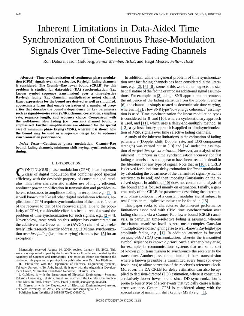
1470 IEEE TRANSACTIONS ON SIGNAL PROCESSING, VOL. 50, NO. 6, JUNE 2002

Inherent Limitations in Data-Aided TimeSynchronization of Continuous Phase-Modulation

Signals Over Time-Selective Fading ChannelsRon Dabora, Jason Goldberg, Senior Member, IEEE, and Hagit Messer, Fellow, IEEE

Abstract—Time synchronization of continuous phase modula-tion (CPM) signals over time selective, Rayleigh fading channelsis considered. The Cramér–Rao lower bound (CRLB) for thisproblem is studied for data-aided (DA) synchronization (i.e.,known symbol sequence transmission) over a time-selectiveRayleigh fading (i.e., Gaussian multiplicative noise) channel.Exact expressions for the bound are derived as well as simplified,approximate forms that enable derivation of a number of prop-erties that describe the bound’s dependence on key parameterssuch as signal-to-noise ratio (SNR), channel correlation, samplingrate, sequence length, and sequence choice. Comparison withthe well-known slow fading (i.e., constant) channel bound isemphasized. Further simplifications are obtained for the specialcase of minimum phase keying (MSK), wherein it is shown howthe bound may be used as asequence design toolto optimizesynchronization performance.

Index Terms—Continuous phase modulation, Cramér–Raobound, fading channels, minimum shift keying, synchronization,timing.

I. INTRODUCTION

CONTINUOUS phase modulation (CPM) is an importantclass of digital modulation that combines good spectral

efficiency with the desirable property of constant signal mod-ulus. This latter characteristic enables use of highly efficient,nonlinear power amplification in transmission and provides in-herent robustness to amplitude fading in reception, e.g., [1]. Itis well known that like all other digital modulation schemes, ap-plication of CPM requires synchronization of the time referenceof the receiver to that of the received signal. Due to the popu-larity of CPM, considerable effort has been directed toward theproblem of time synchronization for such signals, e.g., [2]–[4].Nevertheless, most work on this subject has concentrated onthe additive white Gaussian noise (AWGN) channel with rela-tively little research directly addressing CPM time synchroniza-tion overfast fading(i.e., time-varying) channels (see [5] for anexception).

Manuscript received August 14, 2000; revised January 15, 2002. Thiswork was supported in part by the Israeli Science Foundation founded by theAcademy of Sciences and Humanities. The associate editor coordinating thereview of this paper and approving it for publication was Dr. Inbar Fijalkow.

R. Dabora was with the Department of Electrical Engineering-Systems,Tel Aviv University, Tel Aviv, Israel. He is now with the Algorithms Develop-ment Group, Millimetrix Broadband Networks, Tel Aviv, Israel.

J. Goldberg is with the Department of Electrical Engineering—Systems,Tel Aviv University, Tel Aviv, Israel, and also with the Cellular Communica-tions Division, Intel, Petach Tikva, Israel (e-mail: jason@eng.tau.ac.il).

H. Messer is with the Department of Electrical Engineering—Systems,Tel Aviv University, Tel Aviv, Israel (e-mail: messer@eng.tau.ac.il).

Publisher Item Identifier S 1053-587X(02)04397-0.

In addition, while the general problem of time synchroniza-tion over fast fading channels has been considered in the litera-ture, e.g., [2], [6]–[8], some of this work either neglects the sta-tistical nature of the fading or imposes additional signal assump-tions. For example, in [2], a high SNR approximation removesthe influence of the fading statistics from the problem, and in[6], the channel is simply treated as deterministic time varying,whereas in [8], a low SNR type “low energy coherence” assump-tion is used. Time synchronization for linear modulation typesis considered in [9] and [10], where a cyclostationary approachis used, and [11], which uses a delay-and-multiply method. In[12], a cyclostationary approach is applied to blind synchroniza-tion of MSK signals over time selective fading channels.

A study of the inherent limitations in the estimation of fadingparameters (Doppler shift, Doppler rate, and LOS componentstrength) was carried out in [13] and [14] under the assump-tion ofperfect time synchronization. However, an analysis of theinherent limitationsin time synchronization accuracy for fastfading channels does not appear to have been treated in detail inthe literature for any type of signal. Note that in [10], a CRLBis derived for blind time-delay estimation forlinear modulationby calculating the covariance of the transmitted signal (which isrestricted to be real) and then imposing Gaussianity on the re-ceived signal. In addition, [10] does not contain an analysis ofthe bound and is focused mainly on estimation. Finally, a gen-eral study of the CRLB for parameters describing the determin-istic phase component of a constant modulus signal subject toreal Gaussian multiplicative noise can be found in [15].

This paper seeks to characterize the inherent performancelimitations associated with CPM time synchronization overfading channels via a Cramér–Rao lower bound (CRLB) anal-ysis. In particular, time-selective fading is assumed, whereinthe channel manifests itself as zero mean complex Gaussian“multiplicative noise,” giving rise to well-known Rayleigh-typeamplitude fading, e.g., [1]. In addition, attention is focusedon data-aided (DA)synchronization, wherein the transmittedsymbol sequence is knowna priori. Such a scenario may arise,for example, in communications systems that use some sortof known pilot transmission to synchronize the receiver to thetransmitter. Another possible application is burst transmissionwhere a known preamble is transmitted every burst (or everyfew bursts) to allow correction of the receiver’s reference clock.Moreover, the DA CRLB for delay estimation can also be ap-plied to decision-directed (DD) estimation, where it constitutesa relatively looser lower bound since DD synchronization isprone to bursty type of error events that typically cause a largererror variance. General CPM is considered along with thespecial case of minimum shift keying (MSK) e.g., [1].

1053-587X/02$17.00 © 2002 IEEE

DABORA et al.: INHERENT LIMITATIONS IN DATA-AIDED TIME SYNCHRONIZATION 1471

The paper is structured as follows. Section II reviews CPMand MSK, compares two fast-fading channel correlationmodels, and specifies the overall model for the received data.The problem to be solved is formulated, and the well-knownslow fading channel model is briefly reviewed. In Section III,explicit, exact, and approximate expressions for the CRLB arepresented for both the slow fading and fast fading bounds forgeneral CPM as well as MSK. Section IV derives a variety ofproperties that describe the bound’s dependence on a numberof key parameters such as SNR, channel correlation, andsequence length. Section V presents numerical examples toillustrate the results. Section VI introduces an application of thebound for synchronization sequence design. Last, Section VIIsummarizes the work.

II. M ODELING AND PROBLEM FORMULATION

Begin by considering a general, discrete-time complex base-band signal received over a time-selective fading channel andsampled at sampling interval

(1)

where , , and are the basebandequivalent time-varying channel, transmitted signal, and addi-tive noise components, respectively. The channel componentwill be assumed to be a realization of a zero mean, stationarycircular, complex Gaussian random process

of correlation sequence with. Gaussianity of the channel gives rise to the well-known

Rayleigh distributed amplitude fading. The received signal com-ponent is simply the transmitted signal subject to a delay

. The additive noise is assumed to be a realization of a sequenceof independent, identically distributed (IID) zero mean, circular,complex Gaussian random variables .

Before formulating the exact problem to be solved, CPM isbriefly reviewed, and distinct parametric forms of the channelcorrelation sequence are presented.

A. Continuous Phase Modulation

The continuous time complex envelope of a CPM waveformmay be written as, e.g., [16]

(2)

wheresymbol energy;symbol duration;information bearing phase;arbitrary phase shift (which can be incorporated intothe fading process and is thus taken to be zero).

The information-bearing phase component can be expressed as

(3)

where is an infinitely longsequence of -ary data symbols, each taking one of the values

(4)

where is assumed even. The variableand the functionare referred to as the modulation index and the frequency pulseshape, respectively.

MSK signaling is a special case of CPM formed by settingand while employing the “1REC” frequency

pulse shape

(5)

It is noted that MSK may be viewed as a form of binary con-tinuous-phase frequency shift keying (CPFSK), where one oftwo frequencies and [such that ] istransmitted every seconds. MSK can also be represented interms of linear modulation, e.g., [17]

(6)

where and are the bit period and bit energy, respectively,which, for MSK, satisfy and . As canbe seen, and are generated from the original bitstream by taking only the odd bits for and multiplyingthem with a rectangular pulse train with pulse length of. Thesame is done for with the even bits; however, isalso staggered by with respect to . The relation betweenthe two representations in (3) and (6) is given by .

B. Fading Modeling and Fading Statistics

The Rayleigh fading model is commonly employed inso-called nonline-of-sight (NLOS) propagation conditions,where multiple signal components arrive at the receiverindi-rectly via scattering, diffraction, and reflection effects, e.g.,[1]. If the RMS variation in the arrival time of these channelcomponents is less than a symbol period, then the effect of thechannel can be approximated as purelymultiplicative, givingrise to the model in (1).

Motion of the receiver, the transmitter, or objects present inthe propagation environment all contribute to the time-varyingnature of the channel. Under the zero mean, stationary, circularcomplex Gaussian model of (1), the time-varying nature of thechannel is completely characterized by its correlation sequenceor, equivalently, its Doppler spectrum. A commonly used modelfor land-mobile communications scenarios with isotropic scat-tering and horizontal propagation is the “U-shaped” JakesDoppler spectrum [18]

otherwise

(7)

1472 IEEE TRANSACTIONS ON SIGNAL PROCESSING, VOL. 50, NO. 6, JUNE 2002

where is the maximum Doppler shift in radians per second,which, for the above model, also corresponds to the Dopplerbandwidth . The associated correlation sequence is

(8)

where is the zero-order Bessel function of the first kind.Though common, this representation of the fading process cor-relation was not found to enable derivation of CRLB expres-sions that give analytical insight into the CPM time synchro-nization problem.1 Thus, for the sake of analytical tractability,the channel will be modeled as an autoregressive process (e.g.,[14]) of order one (AR1)2

(9)

where is IID.Although the results obtained with this simplified model are

not numerically identical to the results obtained with the Jakesmodel, theanalyticalinsight obtained under the AR1 model alsoapplies to the Jakes model (see Sections V and VI). Under thismodel, the channel correlation function may be written as

(10)

where is the correlation parameter of the continuous timefading process, and can be viewed as an “effectivecorrelation parameter” induced by the channel as well as thesampling rate. Thus, for , we model the channel as anuncorrelated fading process, and with , we model thechannel as a realization of a single random variable. The cor-responding Doppler spectrum is given by

(11)

where, for this spectrum, the Doppler bandwidth will bedefined as the 3-dB bandwidth of the spectrum, which is easilyshown to be

[Hz] (12)

Note that for both the Jakes and AR1 correlation models, theamplitude of the fading process is Rayleigh distributed, and thephase is uniformly distributed over . To aid in visual-izing the differences between the two models, Fig. 1 presentstheir respective temporal correlation functions. The graphs weredrawn for normalized time-Doppler product of and

. The value of that corresponds to this time-dopplerproduct, when , is . As can beseen from the figure, the correlation produced by the AR1 modellacks the oscillations present in the Jakes model; therefore, thereis no strong peak at , and the spectrum decays more slowlywith frequency.

1While relatively simple, low-order Taylor series approximations of (8) werefound to be of poor accuracy.

2Note that at least for frequency estimation, both [14] and [19] claim that theactual shape of the Doppler spectrum has no noticeable effect on performance.

Fig. 1. Temporal correlation of the fading process forB T = 0:1 for theJakes model and for the AR1 fading correlation model.

C. Statistics of the Received Signal

Assume an observation interval of samples giving rise to, which, from (1), may be written in matrix form as

diag

(13)

with denoting the transpose operation, and diagde-noting a diagonal matrix of specified diagonal elements.Note that the diagonal elements of are the sampledmodulated sequence, which depends on thetransmittedsymbols and on the modulationscheme. For MSK, it is convenient to define abit vector

. We now calculate the statistics ofthe received signal.

Since the transmitted signalis known, of (13) is a sum oftwo zero-mean complex Gaussian random vectors, and hence,

is also a zero-mean complex Gaussian random vector withcorrelation matrix given by

(14)

whereconjugate transposition;

identity matrix,fading channel correlation matrix.

The specific fading channel correlation matrix depends onthe fading statistics. For the AR1 model, use of (10) yields thefollowing correlation matrix:

......

.... . .

...

(15)

DABORA et al.: INHERENT LIMITATIONS IN DATA-AIDED TIME SYNCHRONIZATION 1473

whose inverse will be important in the sequel, e.g., [14]

......

.... ..

...

(16)

It should be noted that such a model was used for the spatialcorrelation in [20] for the case of angle estimation with an arrayof sensors where the data is corrupted byspatialmultiplicativenoise.3

The probability density function (PDF) for the received signalcan now be written as

(17)

where denotes the determinant of a matrix.Before formally stating the problem to be solved, it should

be noted that since it is impossible to distinguish between thefading channel power and the signal power , wewill use to represent their product (i.e., the signal power isnormalized to one) such that SNR is defined as .

D. Estimation Problem

The estimation problem can now be formulated as follows:Given a received signalwith PDF (17), which is parameterizedby an unknown parameter vector, estimate the time delay.In this problem, is the parameter of interest, and the threeremaining parameters arenuisanceparameters.

In the sequel, the results for the fast fading channel will becompared with those of theslow fadingcase described by, e.g.,[21]

(18)

with unknown parameter vector and corre-lation matrix .

III. B OUND EXPRESSIONS

Consider a data vectorand its likelihood function ,which is dependent on a parameter vector. Under a set of reg-ularity conditions, the CRLB for the mean square error of anyunbiased estimator of the th parameter is given by, e.g.,[22]

(19)

where the matrix is known as the Fisher information matrix(FIM), which, for the current statistical model, is given by [22]

tr (20)

3In addition to differences in the parameterization ofS, note that since, in[20], there is no temporal channel correlation, the Fisher information increasesproportionally with time. However, for the temporal problem, this is not thecase; the samples are statistically dependent. Thus, the covariance matrix dimen-sion increases with the sample size, and the increase in the Fisher informationnow depends on “how fast” the channel correlation decreases, which motivatesa specific analysis of the bound for the temporal case.

where tr denotes the trace of a matrix. The remainder of thissection uses (20) and approximations thereof to obtain expres-sions for the CRLB for the time synchronization parameter inslow and fast fading channels.

A. Slow Fading

Recall that parameter vector for the slow fading case of (18)contains three elements: . It is not difficult toshow that the constant modulus property of CPM signal yieldsa FIM of the form [23]4

(21)

which means that the error in the estimation ofis asymptoti-cally uncorrelatedwith the errors of the estimation of the nui-sance parameters and that the bound onmay be written asCRLB . Straightforward calculations indicate that

may be written in a form analogous to that for bearing es-timation, e.g., [23]

(22)

where is the projection matrix onto the subspace orthogonalto the signal subspace (spanned by), and . This im-plies that the bound is determined by the norm of the projectionof on the signal subspace’s orthogonal complement and thatfor minimum error, the derivative of the signal vectorshouldbe orthogonal to the signal vector itself. Note that for asymptot-ically high SNR, the bound tends to zero.

The bound can also be written in terms of the phase as

(23)

which, for MSK, yields, via (6)

(24)

4Note that calculation of the bound on� (for either slow or fast fading) re-quires the elements of the (respective) data covariance to be differentiable withrespect to� . More specifically, the samples of the CPM signal should not occurat times where the complex envelope has no derivative. For MSK, for example,(6), this occurs everyT . Therefore, in general, this analysis is valid for MSK, aslong as the (unsynchronized) receiver does not sample exactly at the transitioninstances (which happens with probability zero). Moreover, many CPM for-mats have continuous derivatives with respect to the time [e.g., Gaussian MSK(GMSK)]; therefore, this question does not even arise.

1474 IEEE TRANSACTIONS ON SIGNAL PROCESSING, VOL. 50, NO. 6, JUNE 2002

B. Fast Fading

Bound expressions for the fast fading case are now presented.Begin by noting that application of the matrix inversion lemmato the data covariance together with the constant modulusproperty of CPM (implying ) yields

(25)

Use of (25) in (20) followed by simple manipulations leadsto the fact that, as in the slow fading case, the asymptotic errorin the delay parameter is decoupled from those of the nuisanceparameters (see Appendix B)

(26)

yielding CRLB . It is emphasized that this result isvalid for any type of fading correlation (e.g., Jakes, AR) whenthe fading process is complex normal and of zero mean. In ad-dition, note that this asymptotic decoupling both in the slow andfast fading scenarios implies that there is no inherent accuracypenalty due to the absence ofa priori knowledge of the signaland noise power (as well as the channel correlation parameterfor the fast fading case). To proceed, a variety of approximationsare now considered.

1) Zero-Order High SNR Approximation:Begin by consid-ering the “zero-order” high SNR approximation to the data co-variance, which is similar to [20] and [24], by simply neglectingthe noise term such that

(27)

Plugging (27) into (20) and using the fact that

(28)

yields the following expression for the FIM element for atasymptotically high SNR:

tr (29)

where . Remembering that ,the following diagonal matrix will be defined:

(30)

such that

(31)

The second element in the trace in (29) yields

(32)

and using tr tr , we can write the first element of(29) as tr tr . Tediousbut straightforward calculations yield a final expression of theform (see Appendix C)

(33)

which can be seen to depend only on the transmitted sequenceand the channel correlation parameter. Most importantly, incontrast to the slow fading case, it is evident from (33) thatthe bound on does notgo to zero for asymptotically highSNR; there is an inherent asymptotic error generated due to therandom fading channel process. It also appears that the boundis not valid when since is a rank one matrix andis, therefore, noninvertible. If it is knowna priori that(corresponding toslow fading), then the CRLB analysis is tobe formulated accordingly as in Section III A.

For MSK, observe that

(34)

Plugging (34) into (29) yields

(35)

where the placement of the factor on the right-hand side of(35) yields a bit period normalized version of the bound. It canbe seen that counts changes in the transmitted I andQ signal components. When there is a change in the bit valuesbetween consecutive samples in either the I or Q components,the associated equals 1; otherwise, equals 1 . De-pending on the transmitted bit sequence, the value ofcan rangebetween for the worst-case sequence and forthe best-case sequence (see Section VI).

2) First-Order High SNR Approximation:A “first-order”high SNR approximation to the inverse of the data covariancecan be obtained by writing the first-order Taylor expansion for

around (similarly to [15] and[20])5

5Actually,� R = (1=�(1� � ))R ,R = � (1� � )R [see(16)], and therefore, the first-order high SNR approximation requires that�(1�� ) ! 1.

DABORA et al.: INHERENT LIMITATIONS IN DATA-AIDED TIME SYNCHRONIZATION 1475

(36)

Now, can be approximated as

(37)

Inserting (37) and (28) in (20) and using the fact thatyields, after simple manipulations

tr (38)

The first-order high SNR expression is seen to be the zero-orderhigh SNR expression minus an SNR dependent term.

3) Low SNR Approximation:First, note that the constantmodulus property enables expression of the inverse of the datacovariance as

A low SNR approximation can be obtained by performing afirst-order Taylor series expansion of about

, yielding

(39)

Plugging (39) and (28) into (20) yields the following low SNRapproximation for the Fisher information:

tr

(40)Using (30) and (31) gives

(41)

Unlike the zero-order high SNR case, depends on SNRand the transmitted sequence.

IV. BOUND PROPERTIES

This section uses the results of the previous section to obtain aseries of bound properties for the slow and fast fading channels.

A. Slow Fading

Property 1: For sufficiently high SNR, the bound on delayestimation for slow fading is approximately inversely propor-tional to SNR.

Proof: Follows from direct inspection of (22).Property 2: The bound on delay estimation for slow fading

is monotonically nonincreasing function of the sample size.Proof: See Appendix D.

B. Fast Fading

Property 1: In contrast to the slow fading case, for low SNR,the fast fading bound is proportional to (decreasingrapidly with SNR), whereas for high SNR, the fast fading boundis proportional to for some constant (decreasingmuch more slowly with SNR).

Proof: The low and high SNR parts of the property followimmediately from (40) and (38), respectively.

Property 2: At high SNR, the bound on delay estimationfor fast fading is monotonically nonincreasing function of thesample size .

Proof: Examining (33), it is seen that appears only inthe signal-dependent factor. Define

(42)

To show that , write

which completes the proof.Property 3: For sufficiently low and sufficiently high SNR,

the bound on delay estimation is a monotonically decreasingfunction of the channel correlation parameter () which variesfrom infinity (at ) to the slow fading bound (at ).

Proof: Monotonicity can be proven directly from (33),which (at least for high SNR) indicates that the bound’s depen-dence on the channel correlation parameter is contained in theterm , which, for , is a monotonicallyincreasing function of .

The fact that the bound tends to infinity at is also seenfrom the above channel-dependent term or, more generally, bythe fact that as , can be approximated assuch that

(43)

where the last equality follows from the constant modulus prop-erty of CPM. This means that as , or, equiva-lently, that the bound is infinite. This property is very intuitivesince, as goes to zero, the channel becomes increasingly morewhite—decorrelating the signal samples to the point where thereis no structure on which an estimator can synchronize.

In the case of asymptotically high SNR, convergence of thefast fading bound to the slow fading bound astends to oneagain follows from the bound term of (33), whichapproaches infinity. This implies that the CRLB tends to zero, asdoes the slow fading bound for asymptotically increasing SNR.

1476 IEEE TRANSACTIONS ON SIGNAL PROCESSING, VOL. 50, NO. 6, JUNE 2002

For low SNR, monotonicity can be proven directly from thefast-fading FIM element for, , which is given by (41).Next, to prove convergence to the slow fading bound, examineagain (41). When approaches 1, (41) becomes

(44)

Inserting as defined in (30), we can write

(45)

Examining expressed in terms of the phase (23)

(46)

we see that as , (since), and the resulting expression is identical to (45), thus

completing proof of the property.Property 4 (for MSK Only):For asymptotically high SNR,

the bound on delay estimation for MSK over a fast-fadingchannel decreases as the sampling rate increases.

Proof: See Appendix A

V. NUMERICAL EXAMPLE

This section presents numerical examples that illustrate thebehavior of the CRLB on as a function of SNR, time-dopplerproduct, sampling rate, and sample size. A nominal MSK modu-lation scenario is considered with a bit rate ofKBPS, a sampling rate of , an AR1 fading channelmodel with (corresponding to ), an SNRof dB, and an alternating bit sequence of lengthbits. Graphs of the exact and approximate forms of the squareroot of the CRLB are plotted as one of the above listed param-eters is varied from its nominal value.

Begin with Fig. 2, which presents a comparison of the boundon delay estimation calculated with the Jakes and the AR1 cor-relation model. Examining the figure, it can be seen that whilethe Jakes bound is lower than the AR1 bound, both exhibit thesametypeof behavior versus SNR. This was also found to bethe case for a wide variety of scenarios (not shown).

Next, Fig. 3 presents the bound on delay estimation versusSNR. Fig. 3(a) plots the bound for SNRs ranging from15to 30 dB, whereas Fig. 3(b) zooms in on the high SNRs.Examining the figure, we observe a slow and fast fadingCRLB dependence on SNR as predicted by Property 1 inSections IV-A and B, respectively. In particular, note how the

Fig. 2. Exact bounds on delay estimation for DA time synchronization with afast fading channel versus SNR size for the Jakes and AR1 correlation modelR = 100 KBPS, SNR= 15 dB,T = (T =2), B T = 0:1.

fast-fading bound decreases more rapidly for low SNR than theslow-fading bound. At higher SNR, however, the fast-fadingbound decreases more slowly than the slow-fading bound. Wecan also see [Fig. 3(b)] that the fast-fading bound arrives atsome nonzero asymptotic value (see Property 1, Section IV-B)for asymptotically increasing SNR, whereas the slow-fadingbound drops to zero as SNR increases. Additionally, weobserve that the first-order high SNR approximation is betterthan the zero-order high SNR approximation for SNRs that arehigher than 14 dB. However, for lower SNRs, the first-orderapproximation yields performance that is far inferior to thatof the zero-order approximation. To understand why, recallthat the zero-order high SNR approximation for the inverse ofthe correlation matrix is . This formula ismeaningful at all SNRs, which implies that the approximatebound will deteriorate gradually as the SNR decreases. Thefirst-order high SNR approximation for the inverse of thecorrelation matrix is . Thisapproximation is better than the zero-order approximationat moderate to high SNR; however, at some point when theSNR decreases, the second term becomes dominant, making

negative definite, which means that the approximationcollapses. The SNR at which the approximation collapses isalso determined by the correlation parameter[we requirethat will be large enough]. At SNRs near the col-lapse of the approximation, the first-order approximation willdeteriorate faster than the zero-order high SNR approximation.Finally, we note that for sufficiently high SNR, the SNR doesnot have a significant effect on the fast-fading bound on delayestimation, and the zero-order high SNR approximation givesquite good results, even for SNRs as low as 10 dB.

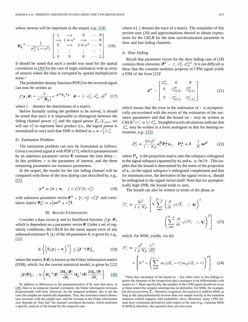
Fig. 4 presents the behavior of the CRLB versus the samplesize . It is seen that as increases, the bound decreasesfor both slow-fading and fast-fading channels, as predicted byProperty 2 in Sections IV-A and B for slow fading and fastfading, respectively. Note that the bound is not necessarily amonotonically decreasing function as in Fig. 4 and that thereare sequences for which the inclusion of additional symbols

DABORA et al.: INHERENT LIMITATIONS IN DATA-AIDED TIME SYNCHRONIZATION 1477

Fig. 3. Bounds on delay estimation for DA time synchronization with a fast-fading channel versus SNR,R = 100 KBPS,K = 31 bits, T = (T =2),B T = 0:1.

Fig. 4. Bounds on delay estimation for DA time synchronization with afast-fading channel versus sample size,R = 100 KBPS, SNR= 15 dB,T = (T =2),B T = 0:1.

will not decrease the bound. We give an example of such a“bad” sequence in Section VI.

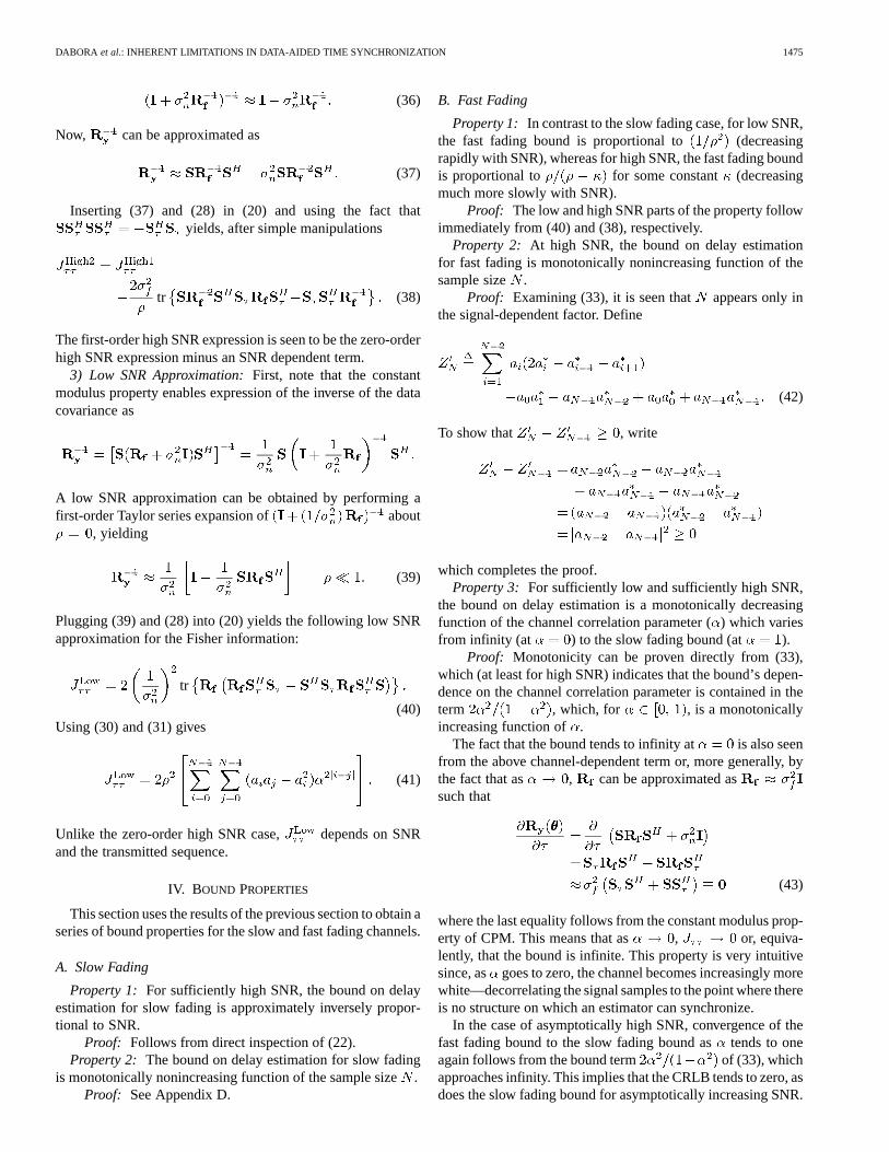
Next, Fig. 5 presents the dependence of the bound on thetime-Doppler product. The figure indicates that the bound in-creases as the time-Doppler product increases. This is consistentwith Property 3 of Section IV-B, which predicts that asin-creases toward unity (i.e., the time-Doppler product approacheszero for fixed bit rate), the bound decreases, whereas asde-creases toward zero (i.e., the time-Doppler product increasesto infinity), the bound increases to infinity. The time-Dopplerproduct has a significant effect on the bound. This is becausethe fading becomes more uncorrelated as increases, suchthat the received signal phase becomes increasingly more white,making it difficult to extract timing information. We also seefrom Fig. 5 that the first-order high SNR approximation breaksdown, even though only is varied, whereas the SNR remainsconstant. The reason is that the first-order high SNR approxi-mation actually requires that will be large enough for

Fig. 5. Bounds on delay estimation for DA time synchronization with afast-fading channel versus time-Doppler product,R = 100 KBPS,K = 31bits,T = (T =2), SNR= 15 dB.

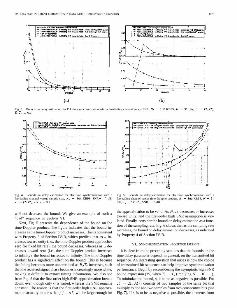
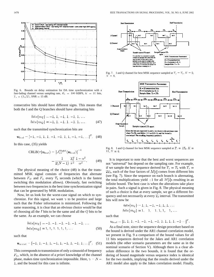
the approximation to be valid. As decreases, increasestoward unity, and the first-order high SNR assumption is vio-lated. Finally, consider the bound on delay estimation as a func-tion of the sampling rate. Fig. 6 shows that as the sampling rateincreases, the bound on delay estimation decreases, as indicatedby Property 4 of Section IV-B.

VI. SYNCHRONIZATION SEQUENCEDESIGN

It is clear from the preceding sections that the bounds on thetime delay parameter depend, in general, on the transmitted bitsequence. An interesting question that arises is how the choiceof transmitted bit sequence can help improve synchronizationperformance. Begin by reconsidering the asymptotic high SNRbound expression (35) when (implying ).To minimize the bound, is to be as negative as possible. For

, consists of two samples of the same bit thatmultiply to one and two samples from two consecutive bits (seeFig. 7). If is to be as negative as possible, the elements from

1478 IEEE TRANSACTIONS ON SIGNAL PROCESSING, VOL. 50, NO. 6, JUNE 2002

Fig. 6. Bounds on delay estimation for DA time synchronization with afast-fading channel versus sampling rate,R = 100 KBPS,K = 31 bits,T = (T =2), SNR= 15 dB.

consecutive bits should have different signs. This means thatboth the I and the Q branches should have alternating bits

(47)

such that the transmitted synchronization bits are

(48)

In this case, (35) yields

CRLB

(49)

The physical meaning of the choice (48) is that the trans-mitted MSK signal consists of frequencies that alternatebetween and every seconds (which is the fastestswitching this modulation allows). Obviously, fast switchingbetween two frequencies is the best time synchronization signalthat can be generated by MSK modulation.

Now, let us look for the worst-case signal on which to syn-chronize. For this signal, we want to be positive and largesuch that the Fisher information is minimized. Following thesame reasoning, it is clear that an obvious choice would be thatof choosing all the bits to be the same and all thebits to bethe same. As an example, we can choose

(50)

such that

(51)

This corresponds to transmission of only a sinusoid of frequency, which, in the absence ofa priori knowledge of the channel

phase, makes time synchronization impossible. Here,, and the bound for this case is infinite.

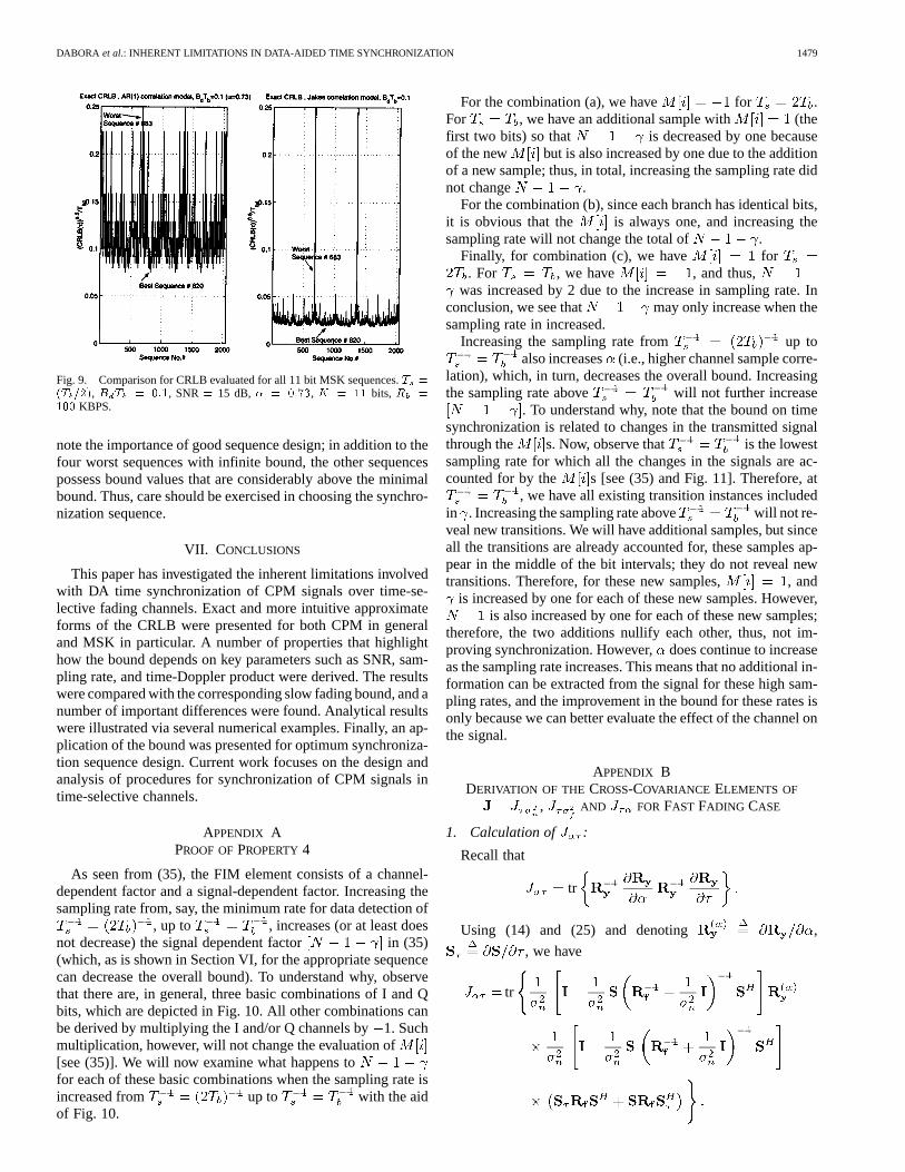
Fig. 7. I and Q channel for best MSK sequence sampled atT = T .K = 9,N = 8.

Fig. 8. I and Q channel for best MSK sequence sampled atT = 2T .K =12,N = 6.

It is important to note that the best and worst sequences arenot “universal” but depend on the sampling rate. For example,if we sample the best sequence derived for with

, each of the four factors of comes from different bits(see Fig. 7). Since the sequence on each branch is alternating,the total multiplications yield 1 for all s resulting in aninfinite bound. The best case is when the alterations take placein pairs. Such a signal is given in Fig. 8. The physical meaningof such a choice is that at every sample, we get a different fre-quency and not necessarily at everyinterval. The transmittedbits will now be

such that

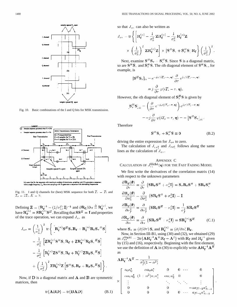
As a final note, since the sequence design procedure based onthe bound is derived under the AR1 channel correlation model,we present in Fig. 9 a comparison of the bound values for all11 bits sequences derived for the Jakes and AR1 correlationmodels (the other scenario parameters are the same as in thenominal scenario of Section V). Although there is a clear ab-solute difference in the two bounds, it is found that the or-dering of bound magnitude versus sequence index is identicalfor the two models, implying that the results derived under theAR1 model also apply to the Jakes correlation model. Finally,

DABORA et al.: INHERENT LIMITATIONS IN DATA-AIDED TIME SYNCHRONIZATION 1479

Fig. 9. Comparison for CRLB evaluated for all 11 bit MSK sequences.T =

(T =2), B T = 0:1, SNR= 15 dB,� = 0:73, K = 11 bits, R =100 KBPS.

note the importance of good sequence design; in addition to thefour worst sequences with infinite bound, the other sequencespossess bound values that are considerably above the minimalbound. Thus, care should be exercised in choosing the synchro-nization sequence.

VII. CONCLUSIONS

This paper has investigated the inherent limitations involvedwith DA time synchronization of CPM signals over time-se-lective fading channels. Exact and more intuitive approximateforms of the CRLB were presented for both CPM in generaland MSK in particular. A number of properties that highlighthow the bound depends on key parameters such as SNR, sam-pling rate, and time-Doppler product were derived. The resultswere compared with the corresponding slow fading bound, and anumber of important differences were found. Analytical resultswere illustrated via several numerical examples. Finally, an ap-plication of the bound was presented for optimum synchroniza-tion sequence design. Current work focuses on the design andanalysis of procedures for synchronization of CPM signals intime-selective channels.

APPENDIX APROOF OFPROPERTY4

As seen from (35), the FIM element consists of a channel-dependent factor and a signal-dependent factor. Increasing thesampling rate from, say, the minimum rate for data detection of

, up to , increases (or at least doesnot decrease) the signal dependent factor in (35)(which, as is shown in Section VI, for the appropriate sequencecan decrease the overall bound). To understand why, observethat there are, in general, three basic combinations of I and Qbits, which are depicted in Fig. 10. All other combinations canbe derived by multiplying the I and/or Q channels by1. Suchmultiplication, however, will not change the evaluation of[see (35)]. We will now examine what happens tofor each of these basic combinations when the sampling rate isincreased from up to with the aidof Fig. 10.

For the combination (a), we have for .For , we have an additional sample with (thefirst two bits) so that is decreased by one becauseof the new but is also increased by one due to the additionof a new sample; thus, in total, increasing the sampling rate didnot change .

For the combination (b), since each branch has identical bits,it is obvious that the is always one, and increasing thesampling rate will not change the total of .

Finally, for combination (c), we have for. For , we have , and thus,

was increased by 2 due to the increase in sampling rate. Inconclusion, we see that may only increase when thesampling rate in increased.

Increasing the sampling rate from up toalso increases (i.e., higher channel sample corre-

lation), which, in turn, decreases the overall bound. Increasingthe sampling rate above will not further increase

. To understand why, note that the bound on timesynchronization is related to changes in the transmitted signalthrough the s. Now, observe that is the lowestsampling rate for which all the changes in the signals are ac-counted for by the s [see (35) and Fig. 11]. Therefore, at

, we have all existing transition instances includedin . Increasing the sampling rate above will not re-veal new transitions. We will have additional samples, but sinceall the transitions are already accounted for, these samples ap-pear in the middle of the bit intervals; they do not reveal newtransitions. Therefore, for these new samples, , and

is increased by one for each of these new samples. However,is also increased by one for each of these new samples;

therefore, the two additions nullify each other, thus, not im-proving synchronization. However,does continue to increaseas the sampling rate increases. This means that no additional in-formation can be extracted from the signal for these high sam-pling rates, and the improvement in the bound for these rates isonly because we can better evaluate the effect of the channel onthe signal.

APPENDIX BDERIVATION OF THE CROSS-COVARIANCE ELEMENTS OF

, AND FOR FAST FADING CASE

1. Calculation of :

Recall that

tr

Using (14) and (25) and denoting ,

, we have

tr

1480 IEEE TRANSACTIONS ON SIGNAL PROCESSING, VOL. 50, NO. 6, JUNE 2002

Fig. 10. Basic combinations of the I and Q bits for MSK transmission.

Fig. 11. I and Q channels for (best) MSK sequence for bothT = T andT = 2T . K = 9.

Defining and , wehave . Recalling that and propertiesof the trace operation, we can expand as

tr

Now, if is a diagonal matrix and and are symmetricmatrices, then

tr tr (B.1)

so that can also be written as

tr

Next, examine . Since is a diagonal matrix,so are and . The th diagonal element of , forexample, is

However, the th diagonal element of is given by

Therefore

(B.2)

driving the entire expression for to zero.The calculation of and follows along the same

lines as the calculation of .

APPENDIX CCALCULATION OF FOR THEFAST FADING MODEL

We first write the derivatives of the correlation matrix (14)with respect to the unknown parameters

(C.1)

where , and .Now, in Section III-B1, using (30) and (32), we obtained (29)

as tr with and givenby (15) and (16), respectively. Beginning with the first element,we use the definition of in (30) to explicitly writeas

......

.... . .

...

DABORA et al.: INHERENT LIMITATIONS IN DATA-AIDED TIME SYNCHRONIZATION 1481

The next step is to multiply this matrix with . Since we per-form the trace operation on the resulting matrix, we will calcu-late only the diagonal elements of

diag

where diag denotes “the diagonal elements of.” The finalstep is to sum these elements with those of (32) resulting in (33)

APPENDIX DPROOF OFPROPERTY2 FOR THESLOW FADING BOUND

We begin with the expressed in term of the phase (23),where for ease of notation, we replacewith . The resulting expression is

(D.1)

Examining this expression, we conclude that in order to provethe property, it is enough to show that

is a nondecreasing function of or, equivalently,, .Begin by writing the difference explicitly

That is

(D.2)

The first two elements can be expanded as

Plugging this back into (D.2), we are now required to prove that

Expanding and then collecting, we get

The last expression is obviously non-negative, implying thatincreasing the number of samples does not decrease the,which proves the property.

1482 IEEE TRANSACTIONS ON SIGNAL PROCESSING, VOL. 50, NO. 6, JUNE 2002

REFERENCES

[1] T. S. Rappaport,Wireless Communications—Principles and Prac-tice. Englewood Cliffs, NJ: Prentice-Hall, 1996.

[2] U. Mengali and A. D’Andrea,Synchronization Techniques for DigitalReceivers (Application of Communication Theory). New York:Plenum, 1997.

[3] U. Mengali, A. N. D’Andrea, and M. Morelli, “Symbol timing esti-mation with CPM modulation,”IEEE Trans. Commun., vol. 44, pp.1362–1371, Oct. 1996.

[4] T. Aulin and C.-E. Sundberg, “Synchronization properties of contin-uous phase modulation,” inProc. Global Telecommun. Conf., Miami,FL, Nov. 1982, pp. D7.1.1–D7.1.7.

[5] F. Patenaude, J. H. Lodge, and P. A. Galko, “Symbol timing trackingfor continuous phase modulation over fast flat-fading channels,”IEEETrans. Veh. Technol., vol. 40, pp. 615–626, Aug. 1991.

[6] K. Goethals and M. Moeneclaey, “Tracking performance of ML-ori-ented NDA symbol synchronizers for nonselective fading channels,”IEEE Trans. Commun., vol. 43, pp. 1179–1184, Feb./Mar./Apr. 1995.

[7] H. L. Van Trees,Detection, Estimation, and Modulation Theory—PartIII . New York: Wiley, 1971.

[8] S. S. Soliman and R. A. Scholtz, “Synchronization over fading disper-sive channels,”IEEE Trans. Commun., vol. 36, pp. 499–505, Apr. 1988.

[9] F. Gini and G. B. Giannakis, “Frequency offset estimation and symboltiming recovery in flat-fading channels: A cyclostationary approach,”IEEE Trans. Commun., vol. 46, pp. 400–411, Mar. 1998.

[10] M. Ghogho, A. Swami, and T. Durrani, “On blind carrier recovery intime-selective fading channels,” inProc. 33rd Asilomar Conf. Signals,Syst., Comput., vol. 1, Pacific Grove, Oct. 1999, pp. 243–247.

[11] K. E. Scott and E. B. Olasz, “Simultaneous clock phase and frequencyoffset estimation,”IEEE Trans. Commun., vol. 43, pp. 2263–2270, July1995.

[12] A. Swami, M. Ghogho, and T. Durrani, “Blind synchronization andDoppler spread estimation for MSK signals in time-selective fadingchannels,” inProc. ICASSP, vol. 5, Istanbul, Turkey, June 2000, pp.2665–2668.

[13] M. Ghogho and A. Swami, “CRB’s and estimators for the parameters oftime selective fading channels,” inProc. SPWAC, Annapolis, MD, May1999, pp. 407–410.

[14] F. Gini, M. Luise, and R. Reggiannini, “Cramer–Rao bounds in the para-metric estimation of fading radiotransmission channels,”IEEE Trans.Commun., vol. 46, pp. 1390–1398, Oct. 1998.

[15] J. M. Francos and B. Friedlander, “Bounds for estimation of multicom-ponent signals with random amplitude and deterministic phase,”IEEETrans. Signal Processing, vol. 43, pp. 1161–1172, May 1995.

[16] T. Aulin and C.-E. W. Sundberg, “Continuous phase modulation—PartI: Full response signaling,”IEEE Trans. Commun., vol. COMM-29, pp.196–209, Mar. 1981.

[17] H. Taub and D. L. Schilling,Principles of Communication Systems, 2nded. New York: McGraw-Hill, 1986.

[18] W. C. Jakes,Microwave Mobile Communications. New York: Wiley,1974.

[19] M. Moeneclaey, H. Meyr, and S. A. Fechtel,Digital CommunicationReceivers: Synchronization, Channel Estimation and Signal Pro-cessing. New York: Wiley, 1997.

[20] O. Besson, F. Vincent, P. Stoica, and A. B. Gershman, “Approximatemaximum likelihood estimators for array processing in multiplicativenoise environments,”IEEE Trans. Signal Processing, vol. 48, pp.2506–2518, Sept. 2000.

[21] C. B. Chang and R. W. Miller, “A modified Cramer–Rao bound andits applications,”IEEE Trans. Inform. Theory, vol. IT-24, pp. 398–400,May 1978.

[22] S. M. Kay,Fundamentals of Statistical Signal Processing: EstimationTheory. Englewood Cliffs, NJ: Prentice-Hall, 1993.

[23] P. Stoica and A. Nehorai, “Performance study of conditional and uncon-ditional direction-of-arrival estimation,”IEEE Trans. Acoust., Speech,Signal Processing, vol. 38, pp. 1783–1795, Oct. 1990.

[24] J. Goldberg, G. Fuks, and H. Messer, “Bearing estimation in a Riceanchannel—Part I: Inherent accuracy limitations,”IEEE Trans. SignalProcessing, vol. 49, pp. 925–937, May 2001.

Ron Daborawas born in Tel Aviv, Israel, in 1972. Hereceived the B.Sc. and M.Sc. degrees, both with highdistinction, in electrical engineering from Tel AvivUniversity in 1994 and 2000, respectively.

Since 2000, he has been with Millimetrix Broad-band Networks, Israel, where he is a member of theAlgorithms Development Group.

Jason Goldberg(SM’99) was born in New Haven,CT, in 1965. He received the B.S.E.E. (with high dis-tinction) and Ph.D. degrees in electrical engineeringfrom Worcester Polytechnic Institute, Worcester,MA, and the University of London, London, U.K.,in 1988 and 1993, respectively.

From 1993 to 1996, he was a PostdoctoralResearcher at Polytechnic University of Catalonia,Barcelona, Spain. Since 1996, he has been aresearcher at Tel Aviv University, Tel Aviv, Israel,in the area of statistical and array signal processing.

In 1998, he also joined the Research Group at the Cellular CommunicationsDivision of Intel, Petach Tikva, Israel, where he works on the design andanalysis of algorithms for wireless communications.

Hagit Messer(F’00) received the B.Sc, M.Sc., and Ph.D. degrees in electricalengineering from Tel Aviv University, Tel Aviv, Israel, in 1977, 1979, and 1984,respectively.

Since 1977, she has been with the Department of Electrical Engi-neering—Systems at the Faculty of Engineering, Tel Aviv University, first asa Research and Teaching Assistant and then, after a one-year post-doctoralappointment at Yale University (from 1985 to 1986), as a Faculty Member.Her research interests are in the field of signal processing and statisticalsignal analysis. Her main research projects are related to tempo-spatial andnon-Gaussian signal detection and parameter estimation.

Dr. Messer was an Associate Editor for the IEEE TRANSACTIONS ONSIGNAL

PROCESSINGfrom 1994 to 1996, and she is now an Associate Editor for the IEEESIGNAL PROCESSINGLETTERS. She is a Member of the Technical Committee ofthe IEEE Signal Processing Society for Signal Processing, Theory, and Methodsand a co-organizer of the IEEE workshop HOS’99. Since 2000, she has been theChief Scientist of the Israeli Ministry of Science, Culture, and Sport.