DESIGN, MODELING, AND CONTROL OF AUTOMOTIVE ...

DESIGN, MODELING, AND CONTROL OF AUTOMOTIVE POWER

TRANSMISSION SYSTEMS

A DISSERTATION

SUBMITTED TO THE FACULTY OF THE GRADUATE SCHOOL

OF THE UNIVERSITY OF MINNESOTA

BY

Xingyong Song

IN PARTIAL FULFILLMENT OF THE REQUIREMENTS

FOR THE DEGREE OF

DOCTOR OF PHILOSOPHY

Professor Zongxuan Sun, Advisor

June, 2011

i

Acknowledgement

I would like to express my sincere gratitude to the people who made a significant

difference in the successful completion of my doctoral study at the University of

Minnesota.

First and foremost, I would like to thank my advisor, Professor Zongxuan Sun, for

the extraordinary vision, competence, dedication, generosity, knowledge and guidance he

provided me throughout my time at the University of Minnesota. I feel forever grateful to

be his first Ph.D. student. His energy and consistent support encouraged me towards

completion of my doctoral study. I sincerely appreciate the invaluable insights and

continuous inspiration provided by him. What’s more, I will never forget the time he

spent in reviewing my research outcome, checking the technical details and proof reading

the paper drafts. Step by step, he taught me how to express logically and concisely, and

demonstrated to me how to become an independent researcher.

I would also like to extend my thanks to my other committee members, Professor

Perry Li, Professor Tryphon Georgiou, and Professor Rajesh Rajamani. I’m sincerely

grateful to Professor Li for his invaluable advice during my research and coursework, and

to Professor Georgiou for his patience whenever I asked questions in his control theory

lecture, and to Professor Rajamani for his very helpful advice when I just came to

University of Minnesota for graduate study. In addition, I also would like to thank

Professor Kim Stelson for serving as my Preliminary exam committee and his time for

evaluating my research proposal. Besides, I also want to thank Dr. Pete Seiler for the

technical discussion on LPV control.

I would also like to acknowledge the financial supports from General Motors

Research Center. And I would like to express my sincere gratitude to Dr. Kumar

Hebbale and Dr. Chi-Kuan Kao in General Motors Research Center for their constructive

comments on my research results.

Besides, I also want to thank my friends and colleagues in my lab, with whom I had

the privilege to work and spend time together, including but not limited to Zhen Zhang,

ii

Yu Wang, Pradeep Gillella, Azrin Zulkefli, Chien-Shin Wu, Ke Li, Adam Heinzen, Ali

Sadighi, and Matt McCuen, etc. I am grateful for their friendship which made my life

easier, happier, and warmer during the long-lasting Minnesota winters

Last but certainly not least, my greatest gratitude goes to my family for their love

and long-lasting support. From my parents, Zhenyuan Song and Lanying Cui, I received

the most encouragement and strength whenever challenges arose. I’m sincerely grateful

for all these years together, and all the happiness we have enjoyed. In addition, my

deepest and sincerest gratitude go to my beloved wife, Shuang Li, for her love,

understanding, devotions, supports, and encouragements during my study. She has

always been an irreplaceable resource of wisdom and strength for me. I feel extremely

fortunate to meet and go through all these incredible years with her together.

iii

Abstract

This thesis focuses on investigating the design, modeling and control methodologies,

which can enable smooth and energy efficient power transmission for conventional,

hybrid and future automotive propulsion systems.

The fundamental requirements of the modern power transmission system are: (1). It

should be able to shift the torque transmission ratio efficiently and smoothly to enable the

fuel efficient operation of the power source. (2). It should be able to reject/damp out the

power source torque oscillation in an energy saving fashion to avoid rough torque

transfer to the driveline. Critical factors determining the successful power transmission

include the appropriate control of the power transfer key components (clutches), the

optimal power transmission coordination with the automotive driveline system, and the

capability to smooth out the power source input oscillation in a fuel efficient fashion. To

meet these resolutions, this thesis will investigate the enabling design and control

methodologies for power transmission in three levels: the fundamental clutch level, the

intermediate driveline level, and the entire propulsion system level.

First, the clutch level design is investigated in two categories: open loop control and

closed loop control. For the open loop, two key issues are addressed. One is to ensure

the consistent initial condition with optimal valve structure design, and the other is the

clutch fill process optimization using a customized dynamic programming with reduced

computational cost for stiff hydraulic system. For the closed loop control case, the

solutions are further divided into two groups. One is to enable feedback with pressure

sensor measurement, and the other is to close the control loop without any sensor.

Through experiments, both methods are shown to enable precise, fast and robust clutch

actuation.

Second, the driveline level design considers optimizing the power transmission

coordination with the driveline. Optimal conditions to achieve efficient and smooth

torque transfer are formulated. The nonlinear optimization is then solved using the

Dynamic Programming.

iv

Finally, in the propulsion system level, the engine start/stop torque oscillation

rejection problem for hybrid vehicle and future advanced combustion system is

discussed. Through proper formulation, this problem can be treated as disturbance

rejection for a linear parameter varying (LPV) system under the internal model principle.

To experimentally implement the state of the art controller design, two problems should

be solved. First, the vibration signal is periodic with changing magnitude, whose

generating dynamics has not been studied before and needs to be derived. Second, the

current linear time varying internal model control is lack of robustness, and the design

method of a low order yet robust internal model stabilizer is still unavailable. This thesis

proposes promising approaches to address this fundamental bottleneck issue in the time

varying internal model control theory, which is one of the key contributions in this thesis.

The proposed stabilizer synthesis method is treated in a general form, and can potentially

be applied to other applications beyond the automotive field as well. Experimental

results are also shown to validate the effectiveness of the proposed algorithm.

In summary, the contributions of this thesis span from the control applications to the

fundamental control theory. Application wise, this thesis formulates the smooth and

efficient power transmission design and control problem in three levels, and proposes

design, dynamics analysis and control methodologies to address the critical challenges in

each level respectively. For control theory, a robust and low order stabilizer synthesis

method is proposed to enable reference tracking/disturbance rejection based on linear

time varying internal model principle. This stabilizer design addresses one of the most

critical issues in the linear time varying internal model control synthesis, which facilitates

experimental investigation of the internal model controller in the LTV setting.

v

Contents

List of Tables xii

List of Figures xiii

Chapter 1 Introduction 1

1.1 Background and Motivation........................................................................ 1

1.2 Research Objectives………………..……………………………….…….. 2

1.3 Dissertation Organization and Overview………………..…………..……. 5

1.4 References in Chapter 1………………..………………..…………..……. 9

Chapter 2 The Clutch Level Design -- Modeling, Analysis

and Optimal Design of the Automotive

Transmission Ball Capsule System 11

2.1 Introduction.................................................................................................. 11

2.2 System Modeling......................................................................................... 14

2.2.1 Dynamic Model…………………………….................................. 15

2.2.2 Derivation of the Throttling Area…………................................... 19

2.2.3 Reduced Order Model………….…………................................... 24

2.3 System Dynamics Analysis......................................................................... 25

2.3.1 Analysis for System with Constant Capsule Angle........................ 25

2.3.2 Analysis for System with Variable Capsule Slope Angle.............. 29

2.4 Optimal Design For the Ball Capsule System............................................. 32

2.4.1 Formulation of Ball Capsule Optimal Design Problem.................. 32

2.4.2 System Model Discretization……………………….………......... 33

vi

2.4.3 Optimal Design Using the Dynamic Programming Method…….. 35

2.5 Case Studies and Simulation Results………............................................... 37

2.6 Conclusion……………………………..………......................................... 43

2.7 References in Chapter 2..……………..………........................................... 45

Chapter 3 The Clutch Level Design -- Transmission Clutch

Fill Control Using a Customized Dynamics

Programming Method 47

3.1 Introduction.................................................................................................. 47

3.2 Problem Description.................................................................................... 50

3.2.1 System Modeling............................................................................ 50

3.2.2 Formulation of the Clutch Fill Control Problem............................ 53

3.3 Optimal Control Design............................................................................... 55

3.3.1 System Model Discretization.......................................................... 56

3.3.2 Applicability of Conventional Numerical Dynamic Programming

to the Optimal Clutch Fill Control.................................................. 56

3.3.3 Optimal Control Using a Customized Dynamic Programming

Method............................................................................................ 57

3.4 Simulation and Experimental Results.......................................................... 63

3.4.1 Experimental Setup…………......................................................... 63

3.4.2 System Identification...................................................................... 64

3.4.3 Clutch Fill Simulation and Experimental Results…...................... 66

3.5 Conclusion................................................................................................... 71


vii

Chapter 4 The Clutch Level Design -- Pressure Based Closed

Loop Clutch Control 77

4.1 Introduction.................................................................................................. 77

4.2 System Dynamics Modeling………………………………………............ 82

4.2.1 Modeling of the Proportional Pressure Reducing Valve................ 83

4.2.2 Mechanical System Modeling…………........................................ 85

4.2.3 Modeling of the Clutch Chamber Pressure Dynamics................... 86

4.2.4 Overall System Dynamics Model................................................... 87

4.3 Robust Nonlinear Controller and Observer Design.................... 90

4.3.1 Sliding Mode Controller Design for Pressure Control…............... 90

4.3.2 Observer Design………………………….………....... 93

4.4 Model Identification and Uncertainty Bound Estimation…………........... 95

4.4.1 Experimental System Description…………………….…............. 96

4.4.2 Pressure Reducing Valve Dynamic Model Identification.............. 97

4.4.3 Mechanical Actuator Dynamic Model Identification..................... 99

4.4.4 Chamber Pressure Dynamic Model Identification......................... 100

4.5 Experimental Result……………………………………………................ 102

4.6 Conclusion………………………………………………………............... 111


Chapter 5 The Clutch Level Design – Design, Modeling and

Control of a Novel Automotive Transmission

Clutch Actuation System 116

5.1 Introduction.................................................................................................. 116

viii

5.2 System Design and Working Principle…..……………………….............. 118

5.2.1 System Design and Working Principle…………………...…........ 118

5.2.2 Advantages of the New Mechanism…........................................... 120

5.3 Mechanical Design and System Modeling…………………….................. 121

5.3.1 Mechanical System Design………………………………............ 121

5.3.2 IFS Modeling……………….……………………………..…....... 122

5.4 Simulation and Experimental Results…………………..……................. 126

5.5 Conclusion……………………………………………............................. 130


Chapter 6 The Driveline Level Design -- Automated Manual

Transmission (AMT) Optimal Clutch Engagement 134

6.1 Introduction.................................................................................................. 134

6.2 System Modeling......................................................................................... 136

6.2.1 Driveline Modeling………………................................................. 136

6.2.2 Clutch Dynamics…….................................................................... 138

6.3 AMT Control System………...................................................................... 139

6.3.1 Engine Control………………........................................................ 139

6.3.2 Gearshift Logic Control.................................................................. 140

6.3.3 Synchronization Control………………………….….................... 140

6.3.4 Clutch Control…………................................................................ 140

6.3.5 Optimal Clutch and Engine Torque During the Clutch

Engagement…………………………………………………….... 143

6.4 Simulation Results and Case Study............................................................. 147

ix

6.5 Conclusion………....................................................................................... 156


Chapter 7 The Propulsion System Level Design -- Tracking

Control of Periodic Signals With Varying

Magnitude And Its Application To Hybrid

Powertrain 160

7.1 Introduction................................................................................................. 160

7.2 Tracking Control of Periodic Signal With Time Varying Amplitude…..... 164

7.3 Application of Amplitude Varying Periodic Signal Repetitive Control on

Hybrid Powertrain Vibration Reduction...................................................... 166

7.3.1 Formulation of the Vibration Rejection Problem........................... 167

7.4 Rotational Angle Based Control……………………………...................... 171

7.4.1 Plant Dynamics Model…...…........................................................ 171

7.4.2 Conversion of the Plant Model to Angle Domain.......................... 173

7.4.3 Internal Model Controller Design…….………….…..................... 174

7.5 Simulation Results………........................................................................... 175

7.6 Conclusion……….……….......................................................................... 180


Chapter 8 The Propulsion System Level Design – Robust

Stabilizer Design for Linear Parameter Varying

(LPV) Internal Model Control System 183

8.1 Introduction.................................................................................................. 183

8.2 Existing Linear Parameter Varying System Control Design

Methods……………………………………………………………….….. 186

x

8.3 Robust Stabilization for LPV Internal Model Controller............................ 189

8.3.1 Preliminaries………………………………………....................... 189

8.3.2 Parameter Dependent Input Gain Injection Problem

Formulation………..………………………………...................... 191

8.3.3 Time Varying Internal Model Stabilization Using Input Gain

Injection…..………..………………………………...................... 192

8.3.4 LMI Formulation to Synthesize Parameter Dependent Input

Injection Gain Vector K(ω)…..…………..………........................ 197

8.3.5 Robust Input Gain Injection Controller Design….......................... 202

8.3.6 Additional Control Gain Constraints…………..…........................ 204

8.4 Experimental Investigation and Results……………….............................. 205

8.4.1 System Dynamics Modeling and Controller Design...................... 207

8.4.2 Experimental Results and Discussion….………........................... 211

8.5 Conclusion……………………………….……………….......................... 217

8.6 Appendix in Chapter 8………………….………………............................ 218


Chapter 9 Conclusion, Contributions Summary and Future

Work 225

9.1 Conclusion…………………………………………................................... 225

9.2 Contributions Summary……………………………………....................... 225

9.2.1 Contributions in Power Transmission Applications....................... 226

9.2.2 Contributions in Control Theory……..….………......................... 227

9.3 Future Work……………………………………………............................ 227

xi

Bibliography 229

xii

List of Tables

2.1. Parameter Values of System Dynamic Model 37

3.1. Parameter Values of the System Dynamic Model 67

4.1 parameter values for system dynamics 103

5.1. System Parameters 130

6.2. The AMT System Dynamic Model Parameters 148

7.1. Parameter Values of the System Dynamic Model 175

8.1. System Parameters 217

xiii

List of Figures

2.1 Automotive Transmission Clutch and Ball Capsule System 13

2.2. Schematic Diagram of the Ball Capsule System 15

2.3. Schematic Diagram of the Ball Capsule System 18

2.4. Fluid centrifugal pressure 18

2.5. Geometric representation of the ball capsule system; a.

Capsule and Ball Geometries; b. Integration of the minimum

distance; c. β and φ relationship 23

2.6. Theoretical and ProE Ath values comparisons 23

2.7. Simulation result comparison between 2nd

and 4th

order model 25

3.1. Scheme diagram of a six speed automatic transmission 48

3.2. Schematic diagram of a clutch mechanism 49

3.3. Stick friction diagram 52

3.4. Desired trajectory of x2 53

3.5. Shifted trajectory of x2 55

3.6. State space quantization 61

3.7: Clutch fill experimental setup 63

3.8. The hydraulic circuit scheme diagram 64

3.9. Experiments for measuring the stick friction Fstatic 65

3.10. System identification model verification 66

3.11. Optimal input pressure and the experimental tracking results 68

xiv

3.12. Experimental results for clutch displacement, velocity and

input flow rate 68

3.13. Clutch fill repeatability test (a). five groups of displacement

profiles. (b) histogram of data error comparing with optimal

trajectory 69

3.14. Clutch fill robustness test 69

3.15. Histogram of clutch fill piston final position 69

3.16. Experimental data demonstrating clutch fill robustness on time delay 70

3.17. Optimal and non-optimal clutch fill velocities profile comparison 71

4.1. Clutch system diagrams; (a). Scheme diagram of a six speed automatic

transmission; (b). Clutch actuation mechanism; (c). Schematic clutch

characteristic curves for dry and wet clutches 78

4.2. Hydraulic circuit diagram of the clutch actuation system 83

4.3. Cross sectional view of the proportional pressure reducing valve 83

4.4. Controller Design Structure 93

4.5. Cross - section of the clutch assembly 96

4.6. Least square approximation of valve parameters 98

4.7. The control valve spool position vs opening orifice area model and its

uncertainty boundary; (a) Input pressure profile; (b) Displacement modeling

error. 99

4.8. Mechanical system identification model verification; (a) Input pressure

profile; (b) Displacement modeling error. 100

4.9. The clutch characteristic curve. ( The wet clutch pack squeezed

displacement vs the corresponding pressure inside the clutch chamber) 100

xv

4.10. Pressure dynamics model matching result 101

4.11. Uncertainty bound of the pressure dynamics model 102

4.12. The experimental setup for pressure based clutch actuation. (Only

pressure is used in the real time feedback, and other sensors are installed for

dynamic modeling purpose.) 104

4.13.The nonlinear observer estimation results; (a) Estimation with accurate

initial state; (b) Estimation with inaccurate initial state 105

4.14. The estimation with clutch fill mechanical dynamics perturbation; (a)

Estimation with low L2 gain in clutch fill; (b) Estimation with high L2 gain in

clutch fill 105

4.15. Pressure tracking for clutch fill and clutch engagement 106

4.16. Control input and the flow-in rate for clutch control; (a). Pressure

control input for clutch fill and clutch engagement; (b). Flow rate for clutch

fill and clutch engagement control 107

4. 17. Successful (a) and failed (b) pressure tracking during the clutch fill 108

4.18. Pressure chattering effect due to large uncertainty bound 109

4.19. Control input and flow rate data; (a). Pressure control input for clutch

fill and clutch engagement; (b). Flow rate for clutch fill and clutch

engagement control 109

5.1 Schematic diagram of transmission clutch system 117

5. 2. IFS system design and working principle; a. Schematic diagram of the

proposed clutch actuation control system; b. Piston and IFS motion during

clutch fill 120

5.3. Feedback control diagram 121

5.4. IFS system mechanical design drawing 124

xvi

5.5. IFS clutch actuation test bed 127

5.6. Multiple tests for clutch piston displacement and the dynamics modeling

error of the clutch piston motion 128

5.7. Intermediate actuation chamber pressure 128

5.8. IFS chamber pressure 128

5.9. IFS spool displacement 129

6.1. The AMT schematic diagram 135

6.2. The clutch operation diagram 139

6.3. The control scheme of AMT system 140

6.4. DP Algorithm 146

6.5. Simulink Model Blocks 148

6.6. Controller Switch Logic 150

6.7. The throttle input and gearshift scheduling 151

6.8. The AMT simulation results 153

6.9. Trajectories of ωc and ωe 154

6.10. Optimal trajectory of ωe – ωc 154

6.11. Optimal trajectory of Tc 155

6.12. Optimal trajectory of Te 155

6.17. Energy loss comparison 156

7.1. Schematic Diagram of Hybrid Powertrain 162

7.2. Engine Torque Oscillation in Time and Angle Domain 163

xvii

7.3. Internal Model Controller Construction 166

7.4. Block Diagram of the Hybrid System 167

7.5. Control Block Diagram for vibration reduction 168

7.6. Magnitude Varying Periodic Velocity Variation 169

7.7. Transformed Control Block Diagram for vibration reduction 172

7.8 (a). Engine Speed Profile; 7.8 (b). Tracking Result Using the Generating

Dynamics From Traditional Repetitive Control; 7.8(c). Tracking Result Using

the Developed Generating Dynamics 178

7.9 (a). Steep Engine Speed Profile; 7.9(b). Tracking Result Using the

Generating Dynamics From Traditional Repetitive Control; 7.9(c). Tracking

Result Using the Developed Generating Dynamics 180

8.1. Block diagram of the feedback controller from [5]. 185

8.2. Stabilizer construction for internal model control system 193

8.3. Control loop with unstructured plant dynamics uncertainty 203

8.4 (a). Picture of hydrostatic dynamometer system; 8.4 (b). Schematic

diagram of the hydrostatic dynamometer 207

8.5 Time varying input injection gains 212

8.6 (a). Pressure tracking with 4.8Hz/sec frequency variation rate; 8.6 (b).

Pressure tracking error vs shifted reference; 8.6 (c). Valve control input 215

8.7 (a). Zoom-in view of pressure tracking at the start with 0.79Hz/sec

frequency variation rate; 8.7 (b). zoom-in view at 161 sec; 8.7 (c). zoom-in

view at 173 sec; 8.7 (d). Valve control input for pressure tracking with

0.79Hz/sec frequency variation rate 216

8.8 (a). Tracking failure for aggressive frequency variation reference due to

parameter perturbation ; 8.8 (b). Valve control input 217

1

Chapter 1

Introduction

1.1 Background and Motivation

This thesis focuses on investigating the design, modeling and control methodologies,

which can enable smooth and energy efficient power transmission for conventional,

hybrid and future automotive propulsion systems.

Automotive propulsion system typically involves power generation [1-2]1 and power

transmission [3-5]. The fundamental requirement of any type of automotive propulsion is

smooth propulsion performance, high energy efficiency and low emissions. To fulfill

these requirements, the main challenges are to enable the clean energy conversion of the

power source, and at the same time transfer the power to the driveline in an efficient and

smooth fashion. First, the efficient power generation highly depends on the operation

condition of the power source [1-2]. The typical optimal operation condition of an

engine lies in a small range of torque and speed [4]. While the performance criteria of

the propulsion system require a wide driveline torque output and speed range, it is

inevitable to have an intermediary mechanism [3-8] between the power source (engine)

and the automotive driveline to enable different operating conditions. Second, the

modern and future automotive propulsion systems seek an aggressive energy

management strategy and advanced energy conversion technique [1-2]. These

technologies often result in higher torque oscillation and thus bring in great challenges to

the smooth torque transfer. For example, the optimal energy management strategy for

hybrid powertrain requires frequent start and stop of the engine [9, 10], which could

generate large engine torque pulses and thus cause driveline vibration. Similarly, many

advanced fuel efficient combustion technologies with a short combustion duration, such

as homogenous charge compression ignition (HCCI) [1-2] for future automotive

propulsion, will generate large torque pulsations and have the same issue for triggering

1 The reference number refers to the reference lists at the end of each chapter. This applys to all the

reference numbers throughout the thesis.

2

driveline vibrations. Clearly, without a smooth power transmission means, those

advanced technologies cannot be effectively implemented.

Therefore, the fundamental requirements of the modern power transmission system

are: (1). It should be able to shift the torque transmission ratio efficiently and smoothly to

enable the fuel efficient operation of the power source. (2). It should be able to

reject/damp out the power source torque oscillation in an energy efficient fashion to

avoid rough torque transfer to the driveline. To meet these two objectives, various kinds

of power transmission devices have been developed. Emerging technologies [3, 4] such

as six or more speeds automatic transmission (AT), continuously variable transmission

(CVT), dual clutch transmission (DCT), automated manual transmission (AMT), and

electrically variable transmission (EVT) have appeared in the market. The newly

developed hybrid power train technology is in fact an electrically variable transmission,

which can optimize the engine operation condition with the aid of electric

motors/generators. However, with these transmission technologies, the system dynamics

become much more complicated. What’s more, the advanced combustion (HCCI, etc) of

current liquid fuel or even the alternative fuel will bring in more critical control

challenges on the future power transmission. Therefore, with the stringent emission and

fuel economy requirements, it becomes increasingly important to incorporate appropriate

feedback control methodologies in the system propulsion and power transfer. This

incorporation not only lies in the appropriate control algorithm, but could also be the

mechanical/hydraulic design aided by the feedback control concept.

1.2 Research Objectives

A successful power transmission is determined by many factors. Specifically, it

depends on the operation of its enabling and most fundamental mechanism, such as

transmission clutches; it depends on its optimal coordination with the automotive

driveline system; it also depends on the capability to smooth out the power source input

in a fuel efficient fashion, such as input torque oscillation rejection. In other words, the

actuation of the clutch system itself should be smooth and efficient; the power

transmission coordination with the driveline should be smooth and efficient; and the

power source oscillation rejection should be smooth and efficient as well. Considering

3

these factors, this thesis will investigate the enabling design and control methodologies

for power transmission in three different levels: the fundamental clutch level, the

intermediate driveline level, and the entire propulsion system level. The problems in

each level are unique, but also interconnected.

First of all, as a complex mechanical system, the power transmission system should

maintain the optimal operation itself. This further requires the proper function of the key

components enabling the power transmission. The clutch is one of the critical

components for most power transfer devices, such as the automatic transmission [4-8],

the automated manual transmission [11], dual clutch transmission [12] and even some

hybrid vehicle transmissions [13-15]. They are connected to the engine and the driveline

respectively and the surfaces are covered with friction material. By engaging or

disengaging the clutches, the power source will be either connected or separated from the

driveline. A smooth and efficient control of the clutch actuation is critical; otherwise it

will cause driveline vibration. This thesis will discuss the clutch level design and control

based on a specific example: the clutch to clutch shift problem in a six speed automatic

transmission, while the principle and approaches can be applied to many other types of

transmissions like multi-mode hybrid transmissions. Specifically, we will investigate the

clutch control methods in two categories: open loop and closed loop control.

The benefits of the open loop clutch control are its hardware compactness and low

cost. Its main challenges lie in two aspects: consistent initial condition and optimal

control process. First, typically the clutch motion happens in an extremely short time

(about 0.2 second). To precisely control the optimal process from the start in open loop, it

is crucial to ensure consistent initial condition. It is observed that the design of a so

called ball capsule system is crucial to ensure the initial condition reliability. In this

thesis, the ball capsule system structure and dynamics are analyzed and optimally

designed. Second, to realize the clutch to clutch shift in open loop, the pre-shift process

called clutch fill, which highly affects the later shift and engagement, should be

optimized. The optimization process is challenging as stiff hydraulic dynamics result in

computational intensive optimization. This thesis then presents a customized dynamic

programming algorithm, which can successfully avoid the stiffness problem.

4

In addition, for the closed loop clutch control, the main challenges are to form a

feedback loop in a structurally compact, precise and robust fashion. Two different

approaches are proposed. One method is to close the control loop with a pressure sensor,

while the other method is to form the feedback without any sensor at all. For the pressure

sensor based control, the sensor is mounted in the clutch chamber and then the clutch

motion and torque transfer are controlled based on the pressure regulation using a sliding

mode controller and an observer. For the feedback control with no sensor measurement,

a new clutch control hydra-mechanical mechanism, which includes an internal feedback

structure, is proposed. The closed loop control is based on pure hydra-mechanical

components, and is proved to be precise, robust, and cost efficient.

Second, a successful clutch actuation alone is not enough. Its coordination with the

driveline is another critical factor. Failure in coordination will result in a less efficient or

perturbed power transmission. Specifically, the desired clutch and driveline coordination

should ensure smooth vehicle launch and gearshift without lurch, and minimize energy

loss due to the clutch slip. To achieve this goal, we applied Dynamic Programming

method to design the optimal clutch and engine velocity/torque trajectory during

gearshift. The method is shown to provide optimal solution given non-quadratic cost

function and the nonlinear dynamic model. In particular, in this thesis, we will study the

driveline level control based on the automated manual transmission (AMT) optimal

clutch engagement problem.

Finally, beyond the self regulation, a successful power transmission design should

also enable the efficient operation of the power source and reject the potential driveline

vibration triggered by the input torque pulses. To be specific, the aggressive energy

management of the hybrid powertrain, the advanced clean combustion like HCCI and etc

require a power transmission mechanism with efficient vibration rejection capability. To

realize this, it is necessary to understand the torque output characteristic from the power

source and the driveline resonance dynamics as well. In other words, the oscillation

rejection needs to be investigated from the integrated system level point of view with an

appropriate understanding of the whole propulsion system. As a representative example,

the power split hybrid system [16] is studied in this thesis. The fuel efficient operation of

5

the hybrid vehicle requires frequent start and stop of the engine, which will induce large

engine torque pulses and can easily cause driveline vibration. Thus the power transfer

control with the energy efficient vibration reduction is crucial. Through proper

formulation, this problem can be treated as disturbance rejection for a linear parameter

varying (LPV) system under the internal model principle. To experimentally implement

the state of the art controller design method, two problems should be solved. First, the

vibration signal is periodic with changing magnitude, whose generating dynamics has not

been studied before and needs to be derived. Second, the current state-of-the-art linear

parameter varying (LPV) internal model based control design is lack of robustness, and

the robust internal model stabilizer synthesis is still unavailable. This thesis proposes

promising approaches to address this fundamental issue in the time varying internal

model control theory, which is one of the key contributions in this thesis. The proposed

stabilizer synthesis method is treated in a general form, and can potentially be applied to

other applications beyond the automotive field as well.

1.3 Dissertation Organization and Overview

In summary, this thesis proposes design, dynamics analysis and control

methodologies, which can enable smooth and energy efficient propulsion and power

transfer. The proposed approaches are presented based on specific examples in three

consecutive levels: clutch level, driveline level and propulsion system level. First, the

clutch level design is presented from chapter 2 to chapter 5. Chapter 2 discusses the

consistent initial condition for open loop clutch control. Chapter 3 presents the open loop

clutch control process optimization. Chapter 4 shows the closed loop clutch control with

only pressure feedback. And Chapter 5 introduces a closed loop clutch control method

without any sensor measurement. Second, the driveline level design is presented in

Chapter 6 using the automated manual transmission driveline coordination as an example.

Finally,

The organization of this thesis will be presented in detailed as the following.

Chapter 2: Clutch Level Design (Clutch Fill Initial Condition Control): Ball Capsule

Dynamics Analysis and Optimal Design

6

In this chapter, the ball capsule dynamics is modeled, in which the derivation of the

ball capsule throttling area is considered novel and critical because of its asymmetrical

nature. Following this, the ball capsule’s intrinsic positive feedback structure is also

revealed, which is considered to be the key to realize a fast response. Moreover, through

the system dynamics analysis, the slope angle of the capsule is found to be an effective

control parameter for system performance and robustness. To this end, the optimal shape

of the capsule is designed using Dynamic Programming to achieve the desired

performance.

Chapter 3: Clutch Level Design ( Open Loop Clutch Control Process Optimization):

Optimal Clutch Fill Control Using a Customized Dynamic Programming

In this chapter, we present a systematic approach to evaluate the clutch fill dynamics

and synthesize the optimal pressure profile. First, a clutch fill dynamic model, which

captures the key dynamics in the clutch fill process, is constructed and analyzed. Second,

the applicability of the conventional numerical Dynamic Programming (DP) method to

the clutch fill control problem, which has a stiff dynamic model, is explored and shown

to be inefficient. Thus we developed a new customized DP method to obtain the optimal

and robust pressure profile subject to specified constraints. The customized DP method

not only reduces the computational burden significantly, but also improves the accuracy

of the result by eliminating the interpolation errors. To validate the proposed method, a

transmission clutch fixture has been designed and built in the laboratory. Both simulation

and experimental results demonstrate that the proposed customized DP approach is

effective, efficient and robust for solving the clutch fill optimal control problem.

Chapter 4: Clutch Level Design ( Closed Loop Control With Pressure Feedback)

:Pressure Based Clutch Control for Automotive Transmissions

In this chapter, we investigated the closed loop clutch control enabled by a pressure

sensor in the clutch chamber. The main challenges of the pressure based clutch control lie

in the complex dynamics due to the interactions between the fluid and the mechanical

systems, the on/off behavior of the clutch assembly, the time varying clutch loading

condition, and the required short time duration for a clutch shift. To enable precise

pressure based control, this chapter presents the contributions in three aspects. First, a

7

clutch dynamic model is constructed and validated, which precisely captures the system

dynamics in a wide pressure range. Second, a sliding mode controller is designed to

achieve robust pressure control while avoiding the chattering effect. Finally, an observer

is constructed to estimate the clutch piston motion, which is not only a necessary term in

the nonlinear controller design but also a diagnosis tool for the clutch fill process. The

experimental results demonstrate the effectiveness and robustness of the proposed

controller and observer.

Chapter 5: Clutch Level Design (Closed Loop Control Without Sensor

Measurement): Hydra-mechanical Based Internal Feedback Mechanism

Development for Clutch Control

This chapter considers the closed loop clutch control without electronic sensor

measurement. To address this problem, a new clutch actuation mechanism is proposed,

which realizes an internal feedback structure. The proposed mechanism is novel as it

embeds all the control elements in the orifice area regulation, which successfully solves

the precise and robust control of the hydraulic system with nonlinear dynamics. In this

paper, we first present the working principle of the new clutch actuation mechanism.

Then, the mechanical system design is shown and the system dynamic model is built. To

this end, the proposed internal feedback control mechanism is fabricated and validated in

a transmission testing fixture. The new mechanism performance is finally presented

through a series of simulation and experimental results.

Chapter 6: Driveline Level Design: Automated Manual Transmission Optimal

Clutch Engagement Analysis

In this chapter, the optimal clutch engagement problem for the automated manual

transmission system is formulated. To realize an energy efficient and smooth clutch

engagement, the possibility of using the Dynamic Programming method to generate the

optimal clutch and engine torque control inputs is investigated. In particular, the

controllability of the AMT system is studied to determine the number of control inputs

necessary for the optimal control, and the Dynamic Programming is applied to solve the

optimization problem.

8

Chapter 7: Propulsion System Level: Hybrid Vehicle Vibration Rejection Using

Angle Based Time Varying Repetitive Control

This chapter presents the hybrid vehicle vibration rejection problem. The key

contributions are to formulate the internal model control approach for periodic signal

with magnitude variation, and then apply the angle based repetitive control for LPV plant

to fulfill the energy efficient vibration rejection. By proper formulation, the oscillation

disturbance signal is periodic with magnitude variation. As will be revealed in this

chapter, the generating dynamics of this kind of signals is time varying, and thus simply

embedding its generating dynamics as the internal model controller will no longer ensure

asymptotic performance. To enable successful vibration reduction, the generating

dynamics of this unique signal is first derived, and then its corresponding controller

design method is presented. After a series of simulations and case studies, the proposed

control framework is demonstrated to be a promising solution for the hybrid powertrain

vibration reduction problem.

Chapter 8: Propulsion System Level: Robust Stabilizer Design for Linear

Parameter Varying (LPV) Internal Model Control System

This chapter focuses on a low order robust stabilizer synthesis for a general linear

parameter varying internal model control problem. The existing stabilization approaches

are either lack of robustness or results in too high stabilizer order, which limit the further

studies in experiments. The method proposed in this chapter overcomes this bottleneck

by taking advantage of the unique structure of the time varying internal model control

system. Instead of using a dynamic stabilizer with high order, the approach using a

sequence of time varying gains will be presented. A critical issue addressed is to avoid

the non-convex optimization associated with the time varying gain synthesis and then

convert the stabilizer design into a series of Linear Matrix Inequality (LMI) constraints.

Experimental studies are then conducted on the hydrostatic dynamometer system and

prove the robustness and computational efficiency of the proposed approach.

9

References in Chapter 1

[1] T. Kuo. Valve and fueling strategy for operating a controlled auto-ignition

combustion engine. In SAE 2006 Homogeneous Charge Compression Ignition

Symposium, pp. 11-24, San Ramon, CA, 2006.

[2] T. Kuo, Z. Sun, J. Eng, B. Brown, P. Najt, J. Kang, C. Chang, and M. Chang. Method

of HCCI and SI combustion control for a direct injection internal combustion engine.

U.S. patent 7,275,514, 2007.

[3] Wagner, G., “Application of Transmission Systems for Different Driveline

Configurations in Passenger Cars”, SAE Technical Paper 2001-01-0882.

[4] Sun, Z. and Hebbale, K., “Challenges and Opportunities in Automotive Transmission

Control”, Proceedings of 2005 American Control Conference, Portland, OR, USA,

June 8-10, 2005.

[5] Lee, C.J., Hebbale, K.V. and Bai, S., “Control of a Friction Launch Automatic

Transmission Using a Range Clutch”. Proceedings of the 2006 ASME International

Mechanical Engineering Congress and Exposition, Chicago, Illinois, 2006.

[6] Hebbale, K.V. and Kao, C.-K., “Adaptive Control of Shifts in Automatic

Transmissions”. Proceedings of the 1995 ASME International Mechanical

Engineering Congress and Exposition, San Francisco, CA, 1995.

[7] Bai, S., Moses, R.L, Schanz, Todd and Gorman, M.J. “Development of A New

Clutch-to-Clutch Shift Control Technology”. SAE Technical Paper 2002-01-1252.

[8] Marano, J.E, Moorman, S.P., Whitton, M.D., and Williams, R.L. “Clutch to Clutch

Transmission Control Strategy”. SAE Technical Paper 2007-01-1313/

[9] S. Tomura, Y. Ito, K. Kamichi, and A. Yamanaka. Development of vibration reduction

motor control for series-parallel hybrid system. In SAE Technical Paper Series 2006-

01-1125, 2006.

[10] S. Kim, J. Park, J. Hong, M. Lee and H. Sim. Transient control strategy of hybrid

electric vehicle during mode change. In SAE Technical Paper Series 2009-01-0228,

2009

10

[11] Glielmo, L. Iannelli, L. Vacca, V. and Vasca, F. “Gearshift Control for Automated

Manual Transmissions”, IEEE/ASME Transactions on Mechatronics, VOL 11, No.

1, Feb., 2006.

[12] Zhang, Y., Chen, X., Zhang, X., Jiang, H., and Tobler, W., “Dynamic Modeling and

Simulation of a Dual-Clutch Automated Lay-Shaft Transmission”, ASME Journal of

Mechanical Design Vol. 127, Issue. 2, pp. 302-307, March, 2005.

[13] T. Goro, et al. Development of the hybrid system for the Saturn VUE hybrid. SAE

technical paper 2006-01-1502.

[14] M. Levin, et. al. Hybrid powertrain with an engine-disconnection clutch. In SAE

Technical Paper Series 2002-01-0930, 2002.

[15] T. Grewe, B. Conlon, and A. Holmes. Defining the General Motors 2-Mode Hybrid

Transmission. SAE technical paper 2007-01-0273.

[16] J. Liu, and H. Peng. Modeling and control of a power-split hybrid vehicle. IEEE

Transactions on Control Systems Technology, vol. 16 (6) pp. 1242-1251, 2008.

11

Chapter 2

The Clutch Level Design--Modeling, Analysis and Optimal

Design of the Automotive Transmission Ball Capsule System

This chapter investigates the initial condition control for open loop clutch operation.

To have a precise open loop actuation, it is critical that the initial conditions of the clutch

fill process do not change from cycle to cycle. It will be revealed that the initial

condition consistency depends on a small valve system called ball capsule system. In the

following the modeling, dynamics analysis and optimal design of this miniature valve

system will be presented in detail.

2.1. Introduction

To reduce vehicle fuel consumption and tailpipe emissions, automotive

manufacturers have been developing new technologies for powertrain systems. In the

transmission area, emerging technologies [1, 2] such as six or more speeds automatic

transmission (AT), continuously variable transmission (CVT), dual clutch transmission

(DCT), automated manual transmission (AMT), and electrically variable transmission

(EVT) have appeared in the market. The basic function of any type of automotive

transmissions is to transfer the engine torque to the vehicle with the desired ratio

smoothly and efficiently. The commonly used actuation device for gear shifts in

transmissions is electro-hydraulically actuated clutch. In automatic and hybrid

transmissions, the most common configuration is to use wet clutches with hydraulically

actuated pistons. This is mainly due to the high power density of electro-hydraulic

systems.

Recently with the introduction of six or more speeds automatic transmissions, the

clutch to clutch shift control technology [3-6] has once again attracted a lot of research

and development efforts. This clutch shift control technology is the key enabler for a

compact, light, and low cost automatic transmission design. This technology uses

pressure control valves to control the clutch engagement and disengagement processes of

the oncoming and off-going clutches. A critical challenge for the clutch shift control is the

12

synchronization of the oncoming and off-going clutches, which is highly dependent on

the oncoming clutch fill time.

A schematic diagram of the transmission clutch system is shown in Figure 2.1. To

engage the clutch, high pressure fluid flows into the clutch chamber and pushes the piston

towards the clutch pack until they are in contact. This process is called the clutch fill. At

the end of the clutch fill process, the clutch pack is ready to be engaged to transfer the

engine toque to the vehicle driveline. The difficulty in realizing a precise clutch fill time

lies in the fact that a pressure feedback control loop could not be formed due to the lack

of a pressure sensor inside of the clutch chamber. Therefore, it is necessary to control the

clutch fill in an open loop fashion, which highly depends on the initial conditions of the

clutch system. To control the clutch fill process precisely, it is therefore critical that the

initial conditions of the clutch fill process do not change from cycle to cycle. However, as

the whole clutch system rotates around the central shaft (Figure 2.1), the centrifugal force

will keep a certain amount of fluid at the ceiling of the clutch chamber. The fluid pressure

induced by the rotation of the leftover fluid will push on the piston and will therefore

affect the initial conditions of the clutch fill process in the following cycle. To dissipate

the leftover fluid and subsequently release the centrifugal force induced pressure, a ball

capsule system is introduced and mounted on the clutch chamber as shown in Figure 2.1.

The ball capsule system consists of a ball and a capsule. Together with the whole

clutch system, the capsule rotates around the central shaft (Figure 2.1). The centrifugal

force acting on the ball keeps the ball in contact with the capsule ceiling, so that the ball

can rotate along the capsule inner wall between the open position and the closed position.

The opening and closing of the ball capsule system is controlled by the fluid pressure

inside the clutch chamber and the centrifugal force. When the fluid pressure inside the

chamber is below a specific level, the sum of moments acting on the ball at the contact

point will push the ball to rotate along the capsule inner wall from the closed position to

the open position. The fluid inside the clutch chamber then can flow out to the exhaust

through the opening area between the ball and the inner wall of the capsule. On the other

hand, when the fluid pressure inside the chamber is high enough, the ball will rotate to

the closed position and seal off the exhaust port.

13

The performance of the ball capsule system is crucial for clutch engagement and

disengagement processes. As shown in Figure 2.1, when the clutch disengages, the piston

is pushed to the left by the spring force, and the fluid inside the clutch chamber is

dissipated through the inlet orifice. At this time, the pressure inside the clutch chamber

drops, and the ball capsule needs to open to allow the fluid held by the centrifugal force

at the ceiling of the chamber to flow out to the exhaust. When the clutch fill process

starts, the pressurized fluid enters the clutch chamber through the inlet orifice. When this

happens, the ball needs to close quickly in order to build up the pressure inside of the

clutch chamber. In addition to these requirements, the system also needs to be robust and

able to avoid undesirable ball chattering between the open and closed positions. In this

chapter, the dynamics of the ball capsule system will be modeled and the stability of the

system will be analyzed, in order to provide the optimal capsule design to achieve the

desired performance.

rb

Open PositionExhaust

Fluid Inlet

Piston

Clutch

Chamber

Orifice

Closed Position

Rotational axis

(center of shaft )

Clutch

Pack

Spring

ω

Figure 2.1. Automotive Transmission Clutch and Ball Capsule System

One of the objectives of this study is to realize swift response of the ball capsule

system during clutch engagement and disengagement. Since the clutch fill process

usually takes a fraction of a second [2], the response of the ball capsule system must be

14

fast enough to allow pressure to build up inside the clutch chamber. In order to

understand and characterize the ball dynamics in such a short time period and its effects

on the clutch chamber pressure, the dynamics of the ball capsule system is modeled. The

main challenge in building the dynamic model is deriving the fluid throttling area, which

is the opening area between the ball and the capsule inner wall. Based on the dynamic

model, an intrinsic positive feedback structure in the system is found. This is in fact

desirable since the unstable characteristic of the ball capsule system results in the

exponential increase of the ball rotational speed, which ensures quick response.

Another objective of the ball capsule design is to prevent high impact speed when

the ball closes the exhaust, which will otherwise cause noise and wears. In addition, the

ball capsule system must be robust, in other words, once the exhaust is closed, it should

remain closed until the clutch is disengaged. If there are pressure variations inside of the

chamber, the ball capsule should not open and the ball must not chatter between the open

and closed positions, which will otherwise adversely influence the clutch fill process. By

analyzing the dynamics of the system, it is found that the desired performance can be

realized by a proper design of the capsule inner wall profile. To this end, a robust design

for the ball capsule system with variable slope angles using the dynamic programming

method is proposed.

The rest of this chapter is organized as follows. Section 2.2 presents the system

dynamic model. Section 2.3 analyzes the intrinsic positive feedback structure of the ball

capsule system. Section 2.4 presents the discrete model of the system and formulates the

ball capsule design problem as an optimization problem. To this end, the Dynamic

Programming method is applied to redesign the shape of the ball capsule inner wall.

Section 2.5 presents case studies and simulation results.

2.2. System Modeling

Figure 2.2 shows the schematic diagram of the ball capsule system. The capsule

rotates around the central shaft (see Figure 2.1) together with the clutch system. The

centrifugal force acting on the ball Fc induced by the rotational motion, keeps the ball in

contact with the capsule ceiling. Since the centrifugal force is normally much larger than

the weight of the ball, the following modeling will be based on the assumption that the

15

ball "rolls" without sliding on the capsule wall. When clutch fill starts, the transmission

fluid with pressure PS from the pump enters the clutch chamber through an orifice, Aorf..

P1 is the fluid pressure inside the chamber V1 between the orifice Aorf and the throttling

area Ath. Ath is the smallest opening area between the ball and the capsule inner wall,

which changes with the motion of the ball. P2 is the fluid pressure inside the chamber V2

between the throttling area Ath and the exhaust orifice Aex. If large enough, the pressure

difference between P1 and P2 will overcome the torque induced by the centrifugal force

Fc and pushes the ball to rotate along the capsule inner wall towards the exhaust port

which is the closed position. Pc is the fluid centrifugal pressure induced by the rotation

of the chamber, and the fluid pressure outside of the exhaust is assumed to be

atmospheric, Patm.

Figure 2.2. Schematic Diagram of the Ball Capsule System

2.2.1 Dynamic Model

The ball capsule system model could be expressed as:

16

( ) ( ) ( )

( )

( )

1 2

.

1 1 2

1

.

2 2 3

2

( ) cos ( ) cos sinc eff b c eff b c b

v

Jv P P A r P P A r F r

P q qV

P q qV

θ

α α α

β

β

=

= + − + −

= −

= −

�

�

(2.1)

where

( )1 1

2d orf S

oil

q C A P Pρ

= − (2.2)

( )2 1 2

2d th

oil

q C A P Pρ

= − (2.3)

( )3 2

2d ex c atm

oil

q C A P P Pρ

= + − (2.4)

( )( )2

coseff bA rπ α= (2.5)

( )3 24

3c b steel oil cF r rπ ρ ρ ω= − (2.6)

( ) ( )cos sincp cap b b br r r r rα θ α= − + − (2.7)

22

2

sinsin sin(2 ) 1 sin tan

2 2

( tan )( )sin(2 )cos( )

2 cos sin

lift

th b lift lift

lift b

lift

b

xA r x x

x rx

r

απ α α π α α

π αα α

α α

= ⋅ + ⋅ + ⋅ − ⋅

− +

(2.8)

( ) ( )cos sin cos( )cos( )

tan( ) tan( )

cap b b b bcp b

lift

r r r r rr rx

α θ α αα

α α

− + − − ×− × = = (2.9)

17

θ is the rotational angle of the ball, v is the ball rotational velocity, rb is the radius of the

ball, and α is the angle of the capsule wall. q1, q2 and q3 are the flow rates at the

corresponding orifices. ω is the clutch system rotational speed, rc is the distance from the

center of the ball to the axis of the transmission (shown in Figure 2.3), rcp is the distance

between the contact point C and the capsule axis, and rcap is the capsule radius shown in

Figure 2.2. Aeff in Eq(2.5) is the area on the ball where the forces acting on the ball due to

pressures P1 and P2 are in effect. This is because, the border line between V1 and V2 on

the ball is assumed to be the vertical line that lies on the points where the radius of the

ball is perpendicular to the surface of the capsule ramp. As a result, the sum of P1 and PC

acts on both sides of the shaded surfaces of the ball in Figure 2.2, thus cancelling the

forces acting on both sides of the surfaces. The remaining area, called Aeff, is therefore the

effective area on which P1 and P2 act against each other. Eq(2.6) is the centrifugal force

acting on the ball due to the rotation of the clutch system. The second equation in Eq(2.1)

is the net moment acting on the ball at the contact point of the ball with the capsule ramp,

denoted as point C. The third equation in Eq(2.1) corresponds to the transient pressure

dynamics of P1 in volume V1, as a result of the flow rate in, q1 through Aorf shown in

Eq(2.2) and the flow rate out, q2 through Ath shown in Eq(2.3). Similarly, the fourth

equation in Eq(2.1) is the transient pressure dynamics of P2 in volume V2. Eq (2.8) and

(2.9) are equations to calculate the throttling area Ath, the derivation of which will be

presented in the next session.

Suppose at the initial condition, the ball is at the top corner of the inner surface of the

capsule (Figure 2.3) and the value of rc at this position is rc_initial. By trigonometry, rc can

be expressed as:

( )_ _ sinc c initial c initial br r h r r θ α= − = − (2.10)

18

rb

( )sinbh rθ α=

bs rθ=

α

Axis of capsule

Point of contact

crcr

_initial

rb

Rotational axis

Figure 2.3. Schematic Diagram of the Ball Capsule System

The centrifugal fluid pressure Pc, shown in Figure 2.4, due to the centrifugal force is

a function of rc and can be expressed as:

( )222

2stc

oil

c rrP −= ωρ

where rst is the starting level of the fluid. Considering that the size of the capsule system

is relatively small compared to the transmission system, Pc could be assumed to be

constant.

Figure 2.4. Fluid centrifugal pressure

19

2.2.2 Derivation of the Throttling Area

Most of the throttling areas in fluid system modeling are symmetric [7]. However, in

the ball capsule system, the derivation of the throttling area Ath between the ball and the

capsule inner surface is not straightforward because the ball is not concentric with the

conical capsule.

As shown in Figure 2.5(a), the capsule surface is a cone surface and could be

represented using cone geometry function as:

Cone surface: 2 2 2 2tany z x α+ = (2.11)

Similarly, the ball surface is a sphere surface centered at Oi (xi,yi,0), and could be

represented as:

Sphere surface: 2222 )()(bii

rzyyxx =+−+− (2.12)

The y-component and z-component of a line OP along the cone surface (Figure.

2.5(a)) can be described in terms of the x-component by using the two equations,

Line OP: tan cosy x α β= (2.13)

tan sinz x α β= (2.14)

To find the throttling area Ath, which is the smallest area between the ball (sphere

surface) and the capsule (cone surface), first the minimum distance from the line OP on

the cone surface to the sphere surface need to be obtained. The shortest distance from a

line to a sphere is also the shortest distance from the sphere center to the line minus the

sphere radius (line AD in Figure. 2.5(b)).

As the ball rotates along the ball capsule surface, its center trajectory is represented

as:

tan seci i by x rα α= − (2.15)

The squared distance between point (x, y, z) on line OP and the center of the ball

(xi,yi,0) is

20

2 2 2 2 2 2 2( ) ( ) ( ) ( tan cos ) ( tan sin )i i i id x x y y z x x x y xα β α β= − + − + = − + − + (2.16)

Differentiating equation (2.16) and equating it to zero leads to the nearest point on

the line OP to the center of the ball

2( tan cos )cosi ix x y α β α= + (2.17)

( tan cos )sin cos cosi iy x y α β α α β= + (2.18)

( tan cos )sin cos sini iz x y α β α α β= + (2.19)

The nearest point is denoted as point D, and the shortest distance as OiD.

Substituting equations (2.17-2.19) into (2.16) yields

2 2 2 2 2 2sin 2 sin cos cos (1 sin cos )i i i i iO D x x y yα α α β α β= − + − (2.20)

Subtracting the radius of the ball from OiD results in the shortest distance from the line

OP to the surface of the sphere

i bAD O D r= − (2.21)

The throttling area, which is shown as the shaded area in Figure 2.5(b), can be divided

into infinitely many trapezoidal elements as illustrated by ADEF in Figure 2.5(b). The

lengths of the arcs AF and DE are:

� cosbAF r dα ϕ= ⋅ and � ( )cosiDE O D dα ϕ= ⋅

Therefore the area of the trapezoidal element ADEF can be calculated as

� � ( ) cos cos( ) ( )

2 2

i bDE AF O D rdA AD AD d

α αϕ

+ += ⋅ = ⋅ ⋅ (2.22)

Since OiD is a function of β, the relationship between β and φ need to be derived to

integrate dA. The relationship between the angle β and φ is shown in Figure 2.5(c).

21

BB’ is the cross sectional view of the ball capsule system at point A, which is

perpendicular to the x axis. The inner circle on BB’ represents the cross sectional surface

of the ball, and the outer circle is the cross section of the cone. According to sines law, in

triangle O’O’iA

sin( ) sin( )

' ' 'i iO O O A

ϕ β β−=

Since O’ and O’i are very close in the ball capsule system, φ-β is small. Therefore the

following approximation can be made

sin( ) ( )ϕ β ϕ β− = −

sin( ) sin( )( ) ( ) ( )

' ' ' ' 'i i i

d d dO O O O O A

ϕ β ϕ β β− −= =

Consequently

cos( )' ' 'i i

d d d

O O O A

ϕ β ββ

−=

Hence ' '

[cos( ) 1]'

i

i

O Od d

O Aϕ β β= +

From equation (2.22)

� � ( ) cos cos ' '( ) ( ) [cos( ) 1]

2 2 '

i b i

i

DE AF O D r O OdA AD AD d

O A

α αβ β

+ += ⋅ = ⋅ ⋅ + ⋅

The throttling area then can be calculated as the convolution of dA about the x-axis,

22

2

sinsin sin(2 ) 1 sin tan

2 2

( tan )( )sin(2 )cos( )

2 cos sin

lift

th b lift lift

lift b

lift

b

xA dA r x x

x rx

r

απ α α π α α

π αα α

α α

= = ⋅ + ⋅ + ⋅ − ⋅

− +

∫

Where ααθα csc)cos(csc bbinbilift rrxrxx −−=−=

22

xi is the distance between the cone vertex O and the ball center Oi along the x-axis, xin is

xi value at the initial position and θ is the rotational angle of the ball. By representing xin

using rcap and rb, the above equation for xlift can be transformed into equation (2.9).

To verify the above formula, the throttling areas are drawn and measured in Pro-

Engineer software. Figure 2.6 shows a good match between the Ath values obtained from

ProE and those from Equation (2.8), where yi is the vertical coordinate of the ball center

defined in Equation (2.15).

(a) Capsule and Ball Geometries

23

Figure 2.5. Geometric representation of the ball capsule system

Figure 2.6. Theoretical and ProE Ath values comparisons

(b) Integration of the

minimum distance (c) β and φ relationship

24

2.2.3 Reduced Order Model

By now, the dynamic modeling for the ball capsule system is completed. However,

the Dynamic Programming method, which will be used for the capsule inner wall profile

design later would suffer from heavy computational burden if the order of the system is

high. Thus, it is desirable to reduce the order of the model while still capturing the main

dynamics of the system. Since the bulk modulus of the fluid is significantly larger

compared to the fluid volume, it is reasonable to assume that the volumetric flow rates

are the same across the whole capsule from the orifice to the exhaust (q1=q2=q3),

resulting in a second order model which can be expressed as:

( ) ( )1 2( ) cos sineff b c b

v

Jv P P A r F r

θ

α α

=

= − −

�

� (2.23)

where

22

1 2 222

2 2

2

2 222

2 2

2

1( )

1( ( ))

1

1 (1

orf th

s atm c

ex th exorfth

th ex ex

th

s s atm c

th exorfth

th ex ex

s

orf

ex

A AP P P P

A A AAA

A A A

AP P P P

A AAA

A A A

PA A

A

= + −

+ + +

= − − −

+ +

+

= −

+ +

[ ]2

2

( )

)

s atm c

ex

th

P P P

A

− +

(2.24)

( )2

2 1

orf

s atm c

ex

AP P P P P

A

= − + −

(25)

As validated by a series of simulation results (see Figure 2.7), the second order ball

capsule model has been shown to be a good approximation of the fourth order ball

capsule model, and therefore will be used in the following analysis and design sections.

25

0 0.1 0.2 0.3 0.4 0.5 0.6 0.7 0.8 0.9 10

0.05

0.1

0.15

0.2Angular Position vs time

time (ms)

Angula

r P

ositio

n (

rad) 2nd-order Position

4th-order Position

0 0.1 0.2 0.3 0.4 0.5 0.6 0.7 0.8 0.9 10

100

200

300

400Angular Velocity vs time

time (ms)

Angula

r V

elo

city (

rad/s

)

2nd-order Velocity

4th-order Velocity

Figure 2.7. Simulation result comparison between 2nd and 4th order model

2.3. System Dynamics Analysis

In this section the stability of the ball capsule system is analyzed as it will provide

insight on the design of the system. As can be seen from Figure 2.7, the rotational speed

of the ball continues to increase, which results in a quick response of the ball capsule

system. The reason for the exponentially increasing velocity is due to an intrinsic positive

feedback structure of the system, and the unstable characteristic is the key enabler of the

quick response of the ball capsule system.

2.3.1 Analysis for System with Constant Capsule Angle

In this section only the capsule with a single slope angle is considered (as shown in

Figure 2.2), which is the simplest way to design the capsule system. Since P1 and P2 both

depend on the throttling area Ath, which in turn is determined by θ, the ball capsule

system can be represented as a closed loop feedback system shown in Figure 2.8.

26

( ) ( )1 2( ) cos sin

eff b C b

v

Jv P P A r F r

θ

α α

=

= − −

�

�

( )th

A θ

θ

thA

Figure 2.8. System dynamics of ball capsule system

Suppose the rotational angle θ increases when the ball rotates clockwise to the

exhaust, and decreases when rotating counterclockwise (see Figure 2.2). As θ increases,

Ath decreases (Eq. 2.8 and Eq. 2.9), and consequently P1 goes up (Eq. 2.24), while P2

drops (Eq. 2.25), resulting in the rise of (P1-P2). Furthermore, the centrifugal force Fc will

drop due to the decrease of rc. Pc is assumed to be constant during this process. Based on

the above analysis, it can be seen that the angular acceleration of the ball will increase

(Eq. 2.23), which further propels the increase of v and θ. Therefore v and θ will keep

increasing until the ball reaches the exhaust port. This reveals the physical mechanism of

the unstable dynamics of the ball capsule system, and a proof based on Chetaev’s

theorem [8] is given as follows.

Given a fixed input pressure Ps and a fixed α value, by solving

( ) ( )1 2

0

( ) cos sin 0eff b c b

v

Jv P P A r F r

θ

α α

= =

= − − =

�

� (2.26)

we can get an equilibrium point:

0

0eqx

θ =

Assume θ0 >0.

For the ball capsule system described by (2.23), define a continuously differentiable

function

0( ) ( )V x vθ θ= − (2.27)

27

U

U

θ

v

Br

[ ]0, 0

T

θ

R

R

Figure 2.9. Region for U

As shown in Figure 2.9, the circle Br is a region on the state space around the

equilibrium point [θ0, 0]T with a radius of r, which can be as large as possible. Let the set

U = {x∈Br | V(x) > 0 except at [θ0, 0]T }, containing the first and third quadrants on the

coordinates. The boundary of U is the two coordinate axes, on which V(x)=0. Next, let

the set R = {x∈Br | V(x) < 0}, containing the second and fourth quadrant.

Theorem 1: For every point x inside the state space except the origin [θ0, 0]T,

2

0 0( ) ( ) ( ) 0V x v v v vθ θ θ θ θ= + − = + − >�� (2.28)

Proof: if θ >θ0, based on Equations (2.8) and (2.9), Ath(θ) < Ath(θ0). From Equation

(2.24), P1(θ) > P1(θ0), and from Equation (2.25) P2(θ) < P2(θ0). Therefore,

[P1(θ)-P2(θ)] > [P1(θ0)-P2(θ0)] (2.29)

In addition, from Equation (2.10), rc(θ) < rc(θ0). Then based on Equation (2.6),

Fc(θ) < Fc(θ0) (2.30)

From Equations (2.23), (2.29) and (2.30), it can be concluded that

0( ) ( ) 0Jv Jvθ θ> =� �

Therefore

( ) 0v θ >� , and 2

0 0( ) ( ) ( ) 0V x v v v vθ θ θ θ θ= + − = + − >��

If θ <θ0, using the same approach gives

28

( ) 0v θ <� , and 0( ) 0θ θ− <

so 2

0 0( ) ( ) ( ) 0V x v v v vθ θ θ θ θ= + − = + − >��

If θ =θ0, 2

0 0( ) ( ) 0V x v v vθ θ θ= + − = >�� if v is not equal to zero. If v=0, then ( ) 0V x =� .

Therefore, ( ) 0V x >� for every x in the state space except the origin [θ0, 0]T. ■

Theorem 2: If the initial state is in region U as shown in Figure 2.9, then the state

trajectory x(t) will leave U through the circle Br. If the initial state starts at the axes, then

x(t) will enter region U. If the state is at region R, then x(t) will have three possible

trajectories depending on the system dynamics. It will eventually enter the first quadrant,

or the third quadrant, or stop at the origin [θ0, 0]T, which is the equilibrium point.

Proof: As V(x) is continuously differentiable in the set U and ( ) 0V x >� in U, according to

Chetaev’s theorem [8], any state trajectory x(t) starting in U must leave U through the

circle Br and therefore be unbounded. Hence the origin is unstable.

The trajectory of the state x(t) can also be analyzed if the initial state x0 lies outside

of the region U. Suppose the initial state starts on the axis excluding the origin [θ0, 0]T. In

this case, V(x0)=0 and ( ) 0V x >� , then

00

( ( )) ( ) ( ( )) 0t

V x t V x V x dτ τ= + >∫ � (2.31)

indicates that x(t) will not stay on the axis where V(x)=0 or enter the region R where

V(x)<0. x(t) will then enter the region U where V(x)>0.

If the initial position x0 starts in the second or the fourth quadrant (region R where

V(x)<0), the dynamic state x(t) must leave this region as well. In this case,

0 0( ) ( ) 0V x vθ θ= − < (2.32)

Define a compact set {x∈R and axV −≤)( }, and then the continuous function )(xV� has

a minimum over the compact set, i.e. 0)()( 0

2 >≥−+= γθθvvxV �� [8], where γ,a are

positive numbers. Therefore

txVdxVxVtxVt

γττ∫ +≥+=0

00 )())(()())(( � (2.33)

29

This indicates that x(t) will eventually leave the above defined compact set. Since this can

happen for an arbitrarily small number a , and also noting that the acceleration v� and the

displacement )( 0θθ − have the same sign (as shown in Theorem 1), x(t) will eventually

enter the first quadrant, or the third quadrant, or stop at the origin. ■

The ball capsule system is shown to be unstable from the above analysis. In fact, the

unstable characteristic is crucial for the ball capsule system performance because it

ensures quick response and fast closure of the ball capsule system. Once the input

pressure Ps is large enough, the ball starts to rotate, and will continue with increasing

speed until it stops at the exhaust. However, as the rotational speed continues to increase,

the speed could get too high when the ball reaches the exhaust and causes collision that

may result in wears and noise.

In addition, the ball capsule system should be robust, which means that once it is

closed it should remain closed until the clutch is disengaged. If the pressure inside the

chamber oscillates, the ball capsule should not open and chatter between the open and

closed positions, which otherwise will adversely influence the clutch fill process. When

the ball is at the open position, the input pressure PS required to rotate the ball towards

the exhaust depends on the slope angle of the capsule at the open position. Similarly, at

the closed position, the pressure P1 required to hold the ball in place is also a function of

the capsule slope angle at the exhaust port. To avoid ball chattering, it is desirable to have

different capsule slope angles. Thus, a capsule shape with variable capsule slope angle is

proposed.

2.3.2 Analysis for System with Variable Capsule Slope Angle

If the angle of the capsule inner wall is not constant, then the system will have

multiple equilibrium points as shown in Figure 2.10(a). The multiple equilibrium points

on the state space are shown in Figure 2.10(b). When the ball rotates in region I as shown

in Figure 2.10(a), its states [θ, v]T lie in region I of the state space as shown in Figure

2.10(b). Similarly, when the ball enters region II on the capsule, its states move to region

II of the state space. Region I and Region II are divided into four quadrants respectively

based on the locations of the equilibrium points O1 and O2.

30

Suppose the initial state x0 is on the axis of θ shown in Figure 2.10(b), which means

that the velocity of the ball is zero at the initial condition, then based on theorem 2 the

trajectory of x(t) will move to quadrant 1 with increasing θ and v, which equally means

that the ball rotates in the positive direction with positive velocity in region I of the

capsule. Eventually the ball will leave region I and reach region II as shown in Figure

2.10(a), which corresponds to the state x(t) arriving at point A in Figure 2.10(b). The

angle of the capsule changes, and so does the location of equilibrium point. Therefore the

trajectory of x(t) in region II need to be considered based on the position of the

equilibrium point O2 shown in Figure 2.10(b). As a result, x(t) arrives in the second

quadrant of region II. Then according to Theorem 2, there will be three possible

trajectories of the state x(t), depending on the position of the equilibrium point O2.

Trajectory 1: Based on the analysis in Theorem 2, if x(t) reaches the equilibrium

point O2, then it will stay there assuming no disturbance. In this case, the ball will stay at

the equilibrium point in region II, which is not desirable because the ball would not close

the capsule.

Trajectory 2: If the state x(t) does not stay at the equilibrium point, then x(t) will

either move to the first quadrant or the third quadrant of region II depending on the

location of the equilibrium point O2. If designed properly, x(t) will enter the first quadrant

of region II and continue with increasing speed until the ball reaches the exhaust, and the

final velocity of the ball could be controlled by choosing the position of equilibrium point

O2. This is the desirable trajectory because the equilibrium points can be chosen by

designing the capsule inner wall profile to control the final velocity of the ball before it

reaches the exhaust.

Trajectory 3: If x(t) enters the third quadrant of region II, then based on Theorem 2

it will eventually go back to region I, which means that the ball will rotate backward to

region I on the capsule. Again, the trajectory of x(t) in region I need to be considered

based on the location of O1. Similar to previous analysis, x(t) enters the fourth quadrant

of region I, and may later go to either point E (a point in the first quadrant), point F (a

point in the third quadrant) or the equilibrium point O1, all of which are undesirable as

the ball will not close the exhaust. In particular, if the state x(t) goes to point E, it will

31

move in the first quadrant of region I again, and repeat the paths analyzed previously.

This is the case where the ball oscillates between region I and region II.

Equilibrium point

Positive direction of and vθ

O1

Region I

Region II

O2Equilibrium point

(a) A capsule system with two different slope angles.

θ

v v’

x0

A

B

C

D

E

F

Region I Region II

O1O2

exhaust

Quadrant 1Quadrant 2

Quadrant 3 Quadrant 4

Quadrant 1Quadrant 2

Quadrant 3 Quadrant 4

(b) Coordinates of the state space and the state transit portrait

Figure 2.10. Ball Capsule System with Multiple Slope Angles

From the analyses above, the trajectory of x(t) is determined by the location of the

equilibrium points. According to equation (2.26), the equilibrium point is related to the

32

capsule angle α. Therefore the dynamics of the ball capsule system can be affected by the

capsule slope angle α. In other words, the capsule slope angle α could be regarded as a

control input to the ball capsule dynamic system. Subsequently, it is proposed that the

angle and shape of the capsule are redesigned to obtain the desired performance.

2.4. Optimal Design For the Ball Capsule System

So far, the ball capsule system dynamics have been modeled and analyzed. To

achieve the desired performance, there have to be control means to affect its dynamic

behavior. As shown before, one of the control means is to design the capsule inner wall

profile. In this section, the capsule profile design problem is converted into a nonlinear

optimization problem, and then the Dynamic Programming method is applied to solve it.

2.4.1 Formulation of Ball Capsule Optimal Design Problem

To achieve the desired ball capsule performance, the optimal design is constrained

by the appropriate choice of the initial conditions Xinitial and final conditions Xfinal, which

are chosen to meet specific design requirements. Additionally, among all the ball capsule

profiles satisfying the above constraints, the one that has the minimum change of capsule

slope angle is desirable. This will result in a smooth shape of the capsule wall, which in

turn reduces the manufacturing cost. The total time Tfinal for the ball to move from the

open position to the closed position is also preferred to be as small as possible.

N=Tfinal/∆t is defined as the number of steps from the initial state to the final state.

Note that Tfinal is not predetermined, but needs to be optimized. Now, the ball capsule

design problem is ready to be formulated as an optimization problem that will achieve the

above objectives. The cost function of the optimization problem is:

2 2 2

1 2 3 4

1

( ( ) ( 1)) ( (0) ) ( ( ) ) ( )N

initial final final

k

g k k X X X N X Tλ α α λ λ λ=

= − − + − + − +∑ (2.34)

In particular, the first term of the cost function ensures the increment of the capsule slope

angle to be as small as possible at each time step. The last three terms ensures that the

system will start from the specified initial conditions and reach the desired final

conditions at minimal time Tfinal. λ1, λ2, λ3 and λ4 are the weighting factors. Consequently,

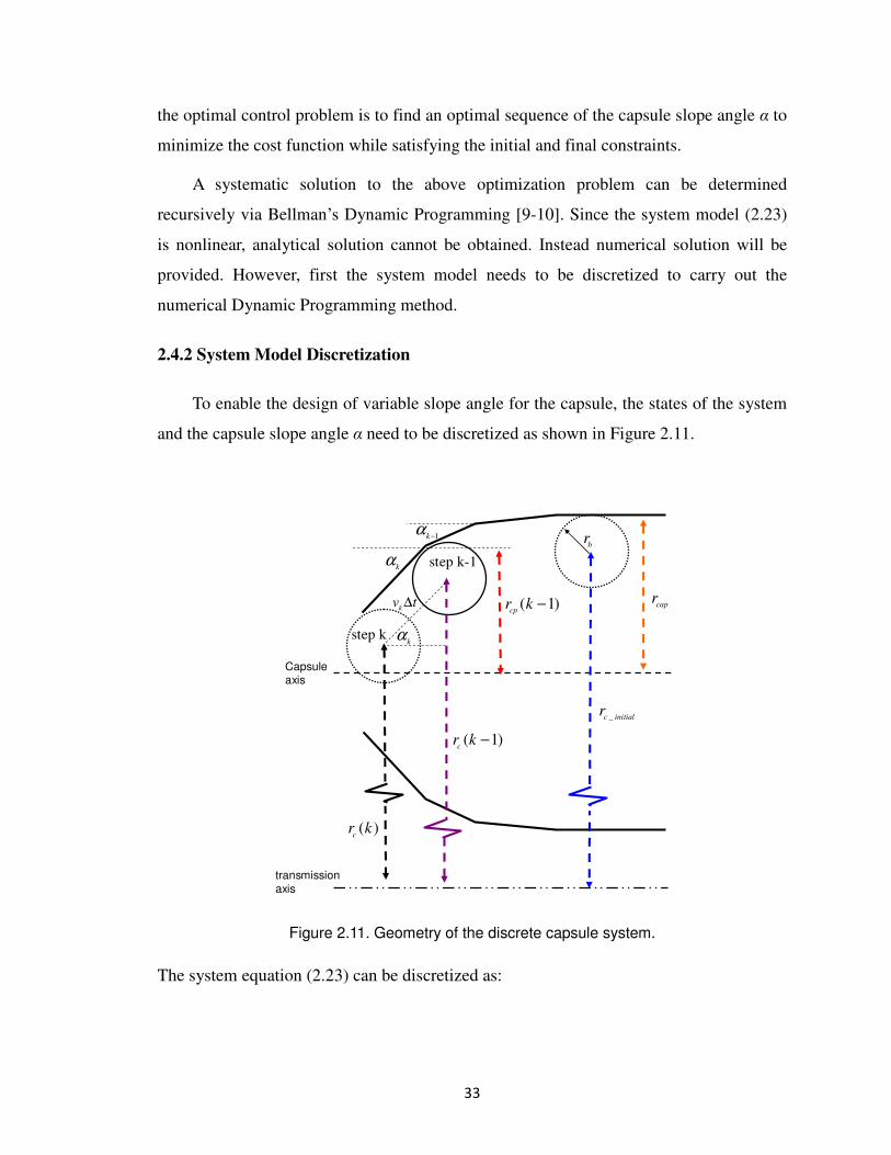
33

the optimal control problem is to find an optimal sequence of the capsule slope angle α to

minimize the cost function while satisfying the initial and final constraints.

A systematic solution to the above optimization problem can be determined

recursively via Bellman’s Dynamic Programming [9-10]. Since the system model (2.23)

is nonlinear, analytical solution cannot be obtained. Instead numerical solution will be

provided. However, first the system model needs to be discretized to carry out the

numerical Dynamic Programming method.

2.4.2 System Model Discretization

To enable the design of variable slope angle for the capsule, the states of the system

and the capsule slope angle α need to be discretized as shown in Figure 2.11.

kα

1kα

−

( )c

r k

capr( 1)

cpr k −

_c initialr

Capsule axis

transmission

axis

br

step k-1

kα

kv t∆

step k

( 1)c

r k −

Figure 2.11. Geometry of the discrete capsule system.

The system equation (2.23) can be discretized as:

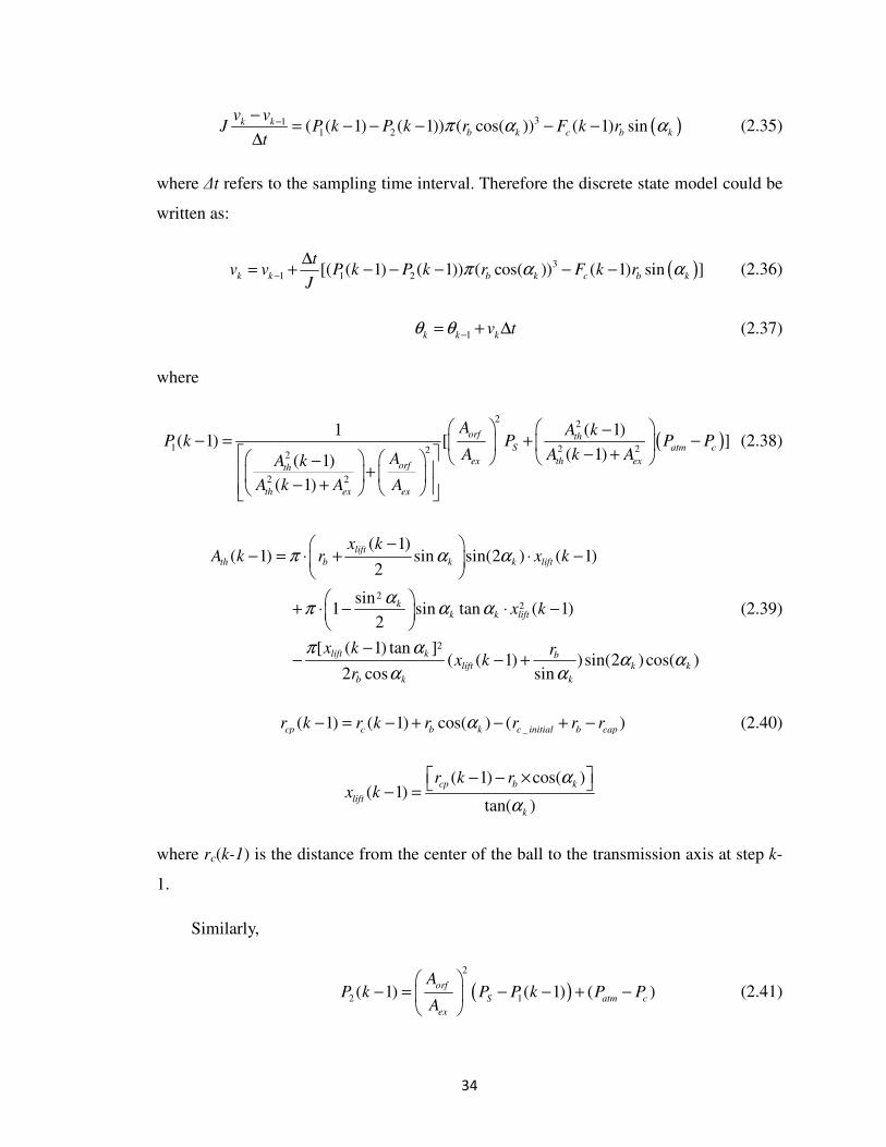
34

( )311 2( ( 1) ( 1)) ( cos( )) ( 1) sink k

b k c b k

v vJ P k P k r F k r

tπ α α−−

= − − − − −∆

(2.35)

where ∆t refers to the sampling time interval. Therefore the discrete state model could be

written as:

( )3

1 1 2[( ( 1) ( 1)) ( cos( )) ( 1) sin ]k k b k c b k

tv v P k P k r F k r

Jπ α α−

∆= + − − − − − (2.36)

1k k kv tθ θ −= + ∆ (2.37)

where

( )2

2

1 2 222

2 2

( 1)1( 1) [ ]

( 1)( 1)

( 1)

orf th

S atm c

ex th exorfth

th ex ex

A A kP k P P P

A A k AAA k

A k A A

−− = + −

− + − +

− +

(2.38)

22

2

( 1)( 1) sin sin(2 ) ( 1)

2

sin1 sin tan ( 1)

2

[ ( 1) tan ]( ( 1) )sin(2 )cos( )

2 cos sin

lift

th b k k lift

k

k k lift

lift k b

lift k k

b k k

x kA k r x k

x k

x k rx k

r

π α α

απ α α

π αα α

α α

− − = ⋅ + ⋅ −

+ ⋅ − ⋅ −

−− − +

(2.39)

_( 1) ( 1) cos( ) ( )cp c b k c initial b cap

r k r k r r r rα− = − + − + − (2.40)

( 1) cos( )( 1)

tan( )

cp b k

lift

k

r k rx k

α

α

− − × − =

where rc(k-1) is the distance from the center of the ball to the transmission axis at step k-

1.

Similarly,

( )2

2 1( 1) ( 1) ( )orf

S atm c

ex

AP k P P k P P

A

− = − − + −

(2.41)

35

3 24( 1) ( ) ( 1)

3c b stl oil c

F k r r kπ ρ ρ ω− = ⋅ − − (2.42)

Finally, rc(k), which is the distance between the center of the ball to the transmission axis

at step k, could be derived if the slope angle αk at step k is known:

( ) ( 1) ( )sin( )c c k k

r k r k v t α= − − ∆ (2.43)

In the discrete model, rc(k) is used to represent the position of the ball.

In summary, equation (2.36) and equation (2.43) together could be expressed as

1[ ( ), ] ( ( 1), , )c k c k k

r k v f r k v α−= − (2.44)

The variable αk, which is the slope angle of the capsule at step k, could be regarded as the

control input.

2.4.3 Optimal Design Using the Dynamic Programming Method

Since in this problem the initial condition is specified instead of the final conditions

(Tfinal needs to be determined), the forward dynamic programming [11], which is a dual

approach to backward dynamic programming [12] is used. The standard numerical

Dynamic Programming approach requires state space discretization and interpolation,

which brings in high computational burden. Therefore the discrete forward dynamic

programming method introduced in [11] is implemented and at the same time the state

space is discretized into regions, which has been presented in [13].

First, at each step k, α is discretized into L discrete values {αk 0

, αk 1

,…αk j…αk

L} as

shown in Figure 2.12. In addition, for each discrete value of αk, discrete regions can be

generated on the plane of rc and v shown as the black and white blocks. According to

equation (2.44), only the predetermined discrete values for αk at each step need to be

generated, and then the values of rc(k-1), vk-1 from previous step together with αk will be

used to obtain the values for rc(k), vk. Then, X(k)=[αk, rc(k), vk]T is defined. As shown in

Figure 2.12, {X0(k-1), X

1(k-1),…X

i(k-1),…X

Lk-1(k-1)} are the possible discrete states

calculated from step k-1. Then suppose from

36

( )[ , ] ( ( 1), ( ))i i i j

c kr k v f X k kα= − (2.45)

rci(k) and vk

i are found and suppose that [αk

j, rc

i(k), vk

i]

T lies in region A in Figure 2.12.

Subsequently, the vector [αk j, rc

i(k), vk

i]

T can be assigned as the value for region A, and

[αk j, rc

i(k), vk

i]

T is memorized as one of the discrete states for step k. Moreover, the cost

function can be calculated based on [αk j, rc

i(k), vk

i]

T as:

2

1 1 1ˆ( , ( ), ) [ ( ) ( ( 1)]j i i j i i

k k c k k k kJ r k v J X kα λ α α − −= − + − (2.46)

In the subsequent calculation, if [αk j, rc

i+c(k), vk

i+c]

T obtained from f(X

i+c(k-1), αk

j) also

falls into region A, then the cost function is recalculated again based on [αk j

, rci+c

(k),

vki+c

]T

as:

2

1 1 1ˆ( , ( ), ) [ ( ) ( ( 1)]j i c i c j i c i c

k k c k k k kJ r k v J X kα λ α α+ + + +

− −= − + − (2.47)

Then if Jk(αk j, rc

i(k), vk

i) is larger than Jk(αk

j, rc

i+c(k), vk

i+c), the value of region A should

be reassigned as [αk j, rc

i+c(k), vk

i+c]

T, and at the same time [αk

j, rc

i(k), vk

i]

T in the discrete

value space would be replaced by [αk j, rc

i+c(k), vk

i+c]

T. But if Jk(αk

j, rc

i(k), vk

i) is smaller

than Jk(αk j

, rci+c

(k), vki+c

), [αk j

, rci+c

(k), vki+c

]T would be discarded and the process

resumes.

Finally, after the minimum cost function for each state has been obtained, it is easy to

get the optimal sequence of capsule slope angle α=[α0,…., αN] which will minimize the

total cost value.

37

v rc

rcv

v

αk0

…...

…...

…...

…...

A

X0(k-1)

Xi(k-1)

Xi+c(k-1)

XLk-1(k-1)

rc

αkj

αkL

αk

Figure 2.12. State space quantization for DP

2.5. Case Studies And Simulation Results

In this section, three possible capsule designs are considered and simulation results

are provided for comparison. The system dynamic model is constructed in

Matlab/SIMULINK environment, and the parameters of the model are shown in Table

2.1.

Table 2.1. Parameter Values of System Dynamic Model

β 17000(bar) ρoil 813.79 (kg/ m3)

Cd 0.7 rst 37.3126 (mm)

ρsteel 7778.05(kg/m3) Aorifice 3.0434 (mm2)

rb 1.9812(mm) ω 2000 (rpm)

Patm 1(bar) rc_initial 56.947 (mm)

Aex 5.8( mm2) rc_final 56.832 (mm)

rcap 2.1 (mm)

The three capsule design profiles are shown in Figure 2.13. The design in Figure

2.13(a), which is the current design of the ball capsule, has a flat surface at the ceiling

38

and an angled wall near the exhaust to hold the ball. Note that, this design can be

considered as a special case of the variable slope angle ball capsule system analyzed in

section 2.3.2. Figure 2.13(b) presents a single slope capsule design，which is analyzed in

section 2.3.1. Figure 2.13(c) shows the optimal capsule design using the Dynamic

Programming method.

The input pressure Ps used in the simulation is 1.2×105

Pa. Figure 2.14 shows the

angular velocity of the ball as it rotates towards the closed position. Figure 2.15 presents

the change of the distance rc , which is the distance between the center of the ball to the

transmission rotational axis, with respect to time. Note that rc at the opening position is

56.947 mm for all three designs, and is 56.832 mm at the exhaust. Figure 2.16 shows the

actuation torque acting on the ball versus time. The actuation torque is defined as

Tor = ( ) ( )1 2( ) cos sineff b c b

P P A r F rα α− − . (2.48)

If the actuation torque is negative at the exhaust, the ball cannot be held at the closed

position and will rotate backward. Figure 2.17 shows the throttling area during the ball

motion.

2.5.1 Case Study I: The Current Capsule Design

For the current capsule design, as shown in Figure 2.14, the ball angular velocity

jumps to a high value, and closes the exhaust quickly. However, at the closed position,

the actuation torque Tor (2.48) is negative as shown in Figure 2.16, which means the ball

could not be held at the exhaust. Thus the ball will rotate backwards, and keep chattering

between the closed position and the open position, which is undesirable for the clutch fill

process. The cause of this chattering phenomenon is the improper design of the slope

angles at the opening position and the closed position. According to the previous analysis

of the system dynamics, the slope angle at the opening position determines the minimum

input pressure Ps (triggering pressure) required to start the ball motion toward the

exhaust, and the slope angle at the closed position determines the minimum input

pressure Ps (holding pressure) required to hold the ball at the exhaust. Figure 2.18 shows

the triggering pressure and holding pressure as a function of the slope angle. It can be

seen that a relatively small input pressure can trigger the start of the ball motion toward

39

the exhaust if the capsule slope angle at the opening position is small (0 degree for

current design). However, if the slope angle at the closed position is large (36.73 degrees

for current design), then the small input pressure will not be enough to hold the ball at the

exhaust, which causes chattering and is exactly the problem associated with the current

capsule design.

2.5.2 Case Study II: The Capsule Design with Single Slope Angle

For the capsule with single slope angle, the ball angular velocity goes up quickly as

shown in Figure 2.14. The angular velocity reaches its peak value before closing off the

exhaust. Note that during the closing process, the throttling area Ath continues to drop,

which acts as the intrinsic feedback to the system dynamics and explains the fast response

of the ball capsule system. Once the capsule is closed, the ball will be held at the closing

position because the actuation torque Tor (2.48) is positive as shown in Figure 2.16.

Therefore this design avoids the chattering problem.

Even though the chattering problem is avoided, the single slope capsule design does

not have any flexibility of controlling the ball capsule system dynamics. If the slope

angle is small, then the ball angular velocity may increase too fast and cause high impact

at the exhaust. In addition, the added length of the capsule due to the small slope angle is

also a concern for packaging. Moreover, as shown in Figure 2.18, if the slope angle is too

large, the triggering pressure will be high, which will waste a lot flow before the ball

capsule can be closed. Another drawback of this design is that, although the single slope

capsule avoids the chattering problem when the input pressure is constant, it does not

ensure robust performance. As shown in Figure 2.18, the difference between the

triggering pressure and the holding pressure is insignificant. Therefore, if there are some

perturbations in the input pressure Ps, the ball will oscillate between the open and closed

positions. Consequently, to add control means to the ball angular velocity and also to

improve system robustness, the capsule design with multiple slope angles is proposed.

40

2.5.3 Case Study III: The Capsule Design with Multiple Slope Angles

To ensure robust performance, the capsule angles at the opening position and at the

exhaust need to be designed appropriately. The capsule angle at the closed position

(Region C in Figure (2.13c)) is designed to be smaller than that at the open position

(Region A in Figure (2.13c)). As shown in Figure (2.18), this design will raise the gap

between minimum triggering pressure and the minimum holding pressure, and thus

increase system robustness. In addition, to avoid noise and wears at the exhaust, the

impact speed at the exhaust is designed to be 200 rad/sec, which is another constraint in

our optimal design. Furthermore, to make manufacturing easier, the number of different

slope angles should be as small as possible. The weighting values selected for the

Dynamic Programming cost function are: λ1=100, λ2=1, λ3=1, λ4=15. Based on the above

constraints, the Dynamic Programming method is used to obtain the optimal values for

the slope angles and the length of each angled section as shown in Figure 2.13 (c).

For the capsule design shown in Figure 2.13 (c), when the ball is closing the capsule,

the ball angular velocity increases initially in region A, because the actuation torque Tor

(2.48) at the beginning is positive as shown in Figure 2.16. When the ball enters region B,

the actuation torque becomes negative due to the large slope angle of region B, resulting

in a decrease in the angular velocity, which is actually the case analyzed in section 2.3.2.

Finally, the ball enters region C and stops at the exhaust. The final angular velocity could

be controlled by designing the slope angles. In addition, as shown in Figure 2.15, the ball

is held at the exhaust, which is ensured by proper design of the slope angles at the open

and closed positions. Again, the intrinsic feedback of the throttling area Ath ensures the

fast closing of the capsule as shown in Figure 2.17.

During clutch disengagement, when the fluid is released from the clutch chamber,

the pressure inside the chamber will drop. When the pressure inside of the clutch chamber

is lower than the minimum pressure to hold the ball at the exhaust, the ball will rotate

back towards the open position. The opening process is also unstable and the rotating

speed of the ball will increase as well. Once the ball reaches the open position (region A),

the centrifugal force will hold the ball at the open position. Since the slope angle at the

open position is designed to be larger than that at the exhaust, the moment from the

41

centrifugal force at the open position will be larger. Moreover, the pressure in the clutch

chamber will be low during the clutch disengagement. Therefore, the centrifugal force

will be large enough to hold the ball still at the open position to avoid ball chattering.

36.73 deg

(a) Current capsule design

(b) Single slope capsule

30 deg

(c) Capsule design from DP

30 deg

40 deg

27.69 deg

A

BC

Figure 2.13. Ball Capsule Design

0 1 2 3 4 5 6 7 8-200

-100

0

100

200

300

400

500

600

Time [mili sec]

velo

cit

y [

ra

d/s

]

The ball angular velocity (rad/s)

current design

single slope

from DP

Figure 2.14. Angular velocity of the ball

42

0 1 2 3 4 5 6 7 856.82

56.84

56.86

56.88

56.9

56.92

56.94

56.96

56.98

Time [mili sec]

rc [

mm

]

The trajectory of the ball center

current design

single slope

from DP

Figure 2.15. The trajectory of the ball center rc

0 1 2 3 4 5 6 7 8-2

0

2

4

6

8

10

12

14

16x 10

-4

Time [mili sec]

To

rq

ue [

Nm

]

The torque(Newton.meter)

current design

single slope

from DP

Figure 2.16. Actuation torque on the ball

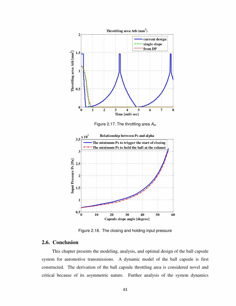
43

0 1 2 3 4 5 6 7 80

0.5

1

1.5

2

Time [mili sec]

Th

ro

ttli

ng

area

Ath

[m

m2]

Throttling area Ath (mm2)

current design

single slope

from DP

Figure 2.17. The throttling area Ath

0 10 20 30 40 50 600.5

1

1.5

2

2.5

3

3.5x 10

5

Capsule slope angle [degree]

Inp

ut

Press

ure P

s [P

a]

Relationship between Ps and alpha

The minimum Ps to trigger the start of closing

The minimum Ps to hold the ball at the exhaust

Figure 2.18. The closing and holding input pressure

2.6. Conclusion

This chapter presents the modeling, analysis, and optimal design of the ball capsule

system for automotive transmissions. A dynamic model of the ball capsule is first

constructed. The derivation of the ball capsule throttling area is considered novel and

critical because of its asymmetric nature. Further analysis of the system dynamics

44

reveals that the ball capsule contains an intrinsic positive feedback structure, and thus is

unstable. This unique and interesting property is the key to ensure a fast response. In

addition, it is found that the shape of the capsule is an effective control parameter for the

performance and robustness of the ball capsule system, and that the capsule with multiple

slope angles rather than the current design could render desired performance. To provide

an optimal design of the ball capsule, the problem is then formulated as a constrained

optimization problem and is solved using Dynamic Programming method. Case studies

and simulation results show the effectiveness of the proposed design methods.

45

References In Chapter 2

[24] Song, X., Zulkefli, A., Sun, Z. and Miao, H., “Transmission Clutch Fill Control

Using A Customized Dynamic Programming Method”, Proceedings of the 2008

ASME Dynamic System and Control Conference, DSCC 2008-2166, Ann Arbor,

Michigan, 2008.


Configurations in Passenger Cars”, SAE Technical Paper 2001-01-0882.

[2] Sun, Z. and Hebbale, K., “Challenges and Opportunities in Automotive Transmission

Control”, Proceedings of 2005 American Control Conference, Portland, OR, USA,

June 8-10, 2005.

[3] Hebbale, K. and Kao, C, “Adaptive Control of Shifts in Automatic Transmissions”,

Proceedings of the 1995 ASME International Mechanical Engineering Congress and

Exposition, San Francisco, CA, 1995.

[4] Bai, S., Moses, R., Schanz, T. and Gorman, M. “Development of A New Clutch-to-

Clutch Shift Control Technology”, SAE Technical Paper 2002-01-1252.

[5] Marano, J., Moorman, S., Whitton, M., and Williams, R. “Clutch to Clutch

Transmission Control Strategy”, SAE Technical Paper 2007-01-1313.

[6] Han, W. and Yi, S., “A Study of Shift Control Using the Clutch Pressure Pattern in

Automatic Transmission”, Proceedings of the IMechE, Part D: Journal of

Automobile Engineering, Volume 217, Number 4/2003, pp 289-298.

[7] Manring, N., 2005, Hydraulic Control Systems, John Wiley & Sons, Hoboken, New

Jersey.

[8] Khalil, H., 2002, Nonlinear Systems (Third Edition), Prentice-Hall Inc., New Jersey.

[9] Bellman, R., 1957, Dynamic Programming, Princeton University Press, New Jersey.

[10] Bellman, R. and Dreyfus, S., 1962, Applied Dynamic Programming, Princeton

University Press, New Jersey.

46

[11] John, H. and Lapidus, L., “Aspects of the Forward Dynamic Programming

Algorithm”, I&EC Process Design and Development, 1968.

[12] Larson, R. and Casti, J., 1978, Principles of Dynamic Programming: Basic

Analytical and Computational Methods, Marcel Dekker Inc., New York and Basel.




Michigan, 2008.

47

Chapter 3

The Clutch Level Design-- Transmission Clutch Fill Control

Using a Customized Dynamic Programming Method

After maintaining a consistent initial condition as presented in Chapter 2, the second

critical factor for the efficient open loop clutch control is the clutch fill actuation process

optimization. In this chapter, we present a systematic approach to evaluate the clutch fill

dynamics and synthesize the optimal control pressure profile.

3.1. Introduction

The automotive transmission, as a key component of the vehicle propulsion system

[1], is designed to transfer the engine torque to the vehicle driveline with desired ratio

smoothly and efficiently. The main components of a typical automatic transmission

include the torque converter, the planetary gear set and the clutch system. The power

transfer and gearshift is in fact realized by engaging and disengaging the clutch systems.

Figure 3.1 shows a simplified schematic diagram of a six speed automatic transmission

[2], with five sets of clutch packs. Clutches are connected to specific gears of the

planetary gear set, and different gear ratio is realized by engaging the corresponding

clutches. During the gear shift, one set of clutch (on-coming clutch) needs to be engaged

and another set (off-going clutch) needs to be disengaged [2], which is called clutch to

clutch shift [3-7]. For a smooth clutch to clutch shift, precise synchronization of the on-

coming clutch and off-going clutch is critical, which otherwise will cause undesirable

torque interruption and oscillation [3]. To ensure precise synchronization, before clutch

engagement, it is necessary to actuate the oncoming clutch to a position where the clutch

packs are just in contact. This process is called clutch fill and plays an important role for

the clutch to clutch shift technology.

48

Figure 3.1. Scheme diagram of a six speed automatic transmission

The commonly used clutch actuation devices in transmissions are electro-

hydraulically actuated clutches. This attributes mainly to the high power density of

electro-hydraulic systems. A schematic diagram of a typical transmission clutch

actuation system is shown in Figure 3.2. Once the clutch is to be engaged, pressurized

fluid flows into the clutch chamber and pushes the clutch piston towards the clutch packs

until they are in contact (clutch fill). At the end of the clutch fill process, the input

pressure Ps is further increased, which then squeezes the clutch piston to the clutch packs

and transfers the engine toque to the vehicle driveline. It is imperative to control the

clutch piston to reach the clutch packs within a specified clutch fill time because an

improper clutch fill process can result in either an under-fill or an over-fill [3], both of

which can cause the failure of the clutch shift synchronization and therefore negatively

affect the clutch shift quality. Therefore, designing the clutch fill pressure command is

critical to achieve a fast and precise clutch fill and a smooth start to the clutch

engagement process. Moreover, it is desirable to synthesize the clutch fill pressure to

reduce the peak flow demand during the clutch fill process. This feature would enable a

smaller transmission pump to improve vehicle fuel economy [8]. However, there are two

main challenges associated with the clutch fill control design. First, even small errors in

calculating the clutch fill pressure and fill time could lead to an over-fill or an under-fill,

which will adversely impact the shift quality. Second, currently there is no pressure

sensor inside the clutch chamber, and consequently a pressure feedback control loop

could not be formed. Therefore, it is necessary to design an open loop pressure control

49

profile, which should be optimal in the sense of peak flow demand and also robust in

terms of clutch fill time. Clearly, the traditional approach based on manual calibration is

not effective to achieve the above objectives. In this chapter, we will present a systematic

approach to solve this problem.

Clutch

Seal

Piston

Return

Spring

pp

ps

Wave

Plate

Piston

Seal

Clutch

Piston

Return

Spring

Orifice

Clutch

Packs

Ps

Pp

xp

Figure 3.2. Schematic diagram of a clutch mechanism

To enable a systematic and model based control design, a precise clutch fill dynamic

model is necessary. It should capture the key dynamics of the clutch fill process, which

are not identical to those of the clutch engagement process [9-11]. Based on the clutch fill

dynamic model, a systematic approach for this control problem can be determined

recursively via Bellman’s Dynamic Programming (DP) method [12-13]. Researchers in

vehicle control field have successfully applied Dynamic Programming to various optimal

control problems [14-16]. For example, Kim and co-authors [15] used Dynamic

Programming (DP) method to obtain the optimal gear shift and throttle control that

maximizes fuel economy while satisfying the power demand. Kang and co-authors [16]

have applied optimal control method to lean burn engines using numerical DP approach.

However, different from applications above, the clutch actuation system contains high

frequency and stiff dynamics [10, 11], which requires a very fast sampling rate for the

discretized model. As a result, the large number of steps, along with the curse of

dimensionality [17] associated with conventional numerical DP method, prohibits its

efficient implementation for the clutch fill control problem. Furthermore, the

conventional numeric DP algorithm suffers from interpolation errors, which will affect

the accuracy of the final results. Therefore, we have proposed a customized numerical

50

Dynamic Programming approach, which has successfully solved the above problems and

generated satisfactory results. The customized DP method transforms the stiff dynamic

model into a non-stiff one by a unique model structure transformation and state

discretization, and thus enables the reduction of the discrete sampling steps.

Furthermore, by discretizing the state space into regions rather than discrete nodes, the

interpolation error is avoided. Finally, the customized DP only searches the optimal

solution within the reachable discrete states, which dramatically reduces the searching

space and therefore mitigates the curse of dimensionality problem [17].

To validate the proposed control methodology, a transmission clutch fixture and

hydraulic control circuit are designed and built to facilitate the experimental investigation

of the optimal clutch fill control. Through a series of experiments, the dynamic model

parameters are identified. To this end, the optimal clutch fill input pressure designed by

the customized dynamic programming is implemented to achieve the optimal clutch fill

performance.

The rest of the chapter is organized as follows. Section 3.2 presents the system

model and formulates the clutch fill control problem as an optimization problem. Section

3.3 first investigates the applicability of conventional numerical Dynamic Programming

approach and then presents the customized numeric DP method. Experimental setup,

system identification and the clutch fill experimental results are presented in section 3.4.

Conclusion is provided in section 3.5.

3.2. Problem description

In this section, we first model the transmission clutch actuation system and then

formulate the clutch fill control problem as an optimization problem.

3.2.1 System Modeling

As shown in Figure 3.2, ps is the supply pressure command and also the control

input to the system, pp is the pressure inside the clutch chamber, and xp is the clutch

piston displacement. The pressurized fluid flows into the clutch chamber and pushes the

clutch piston to the right, and finally contacts the clutch pack. We call this process clutch

fill. The dynamics associated with clutch fill can be modeled as:

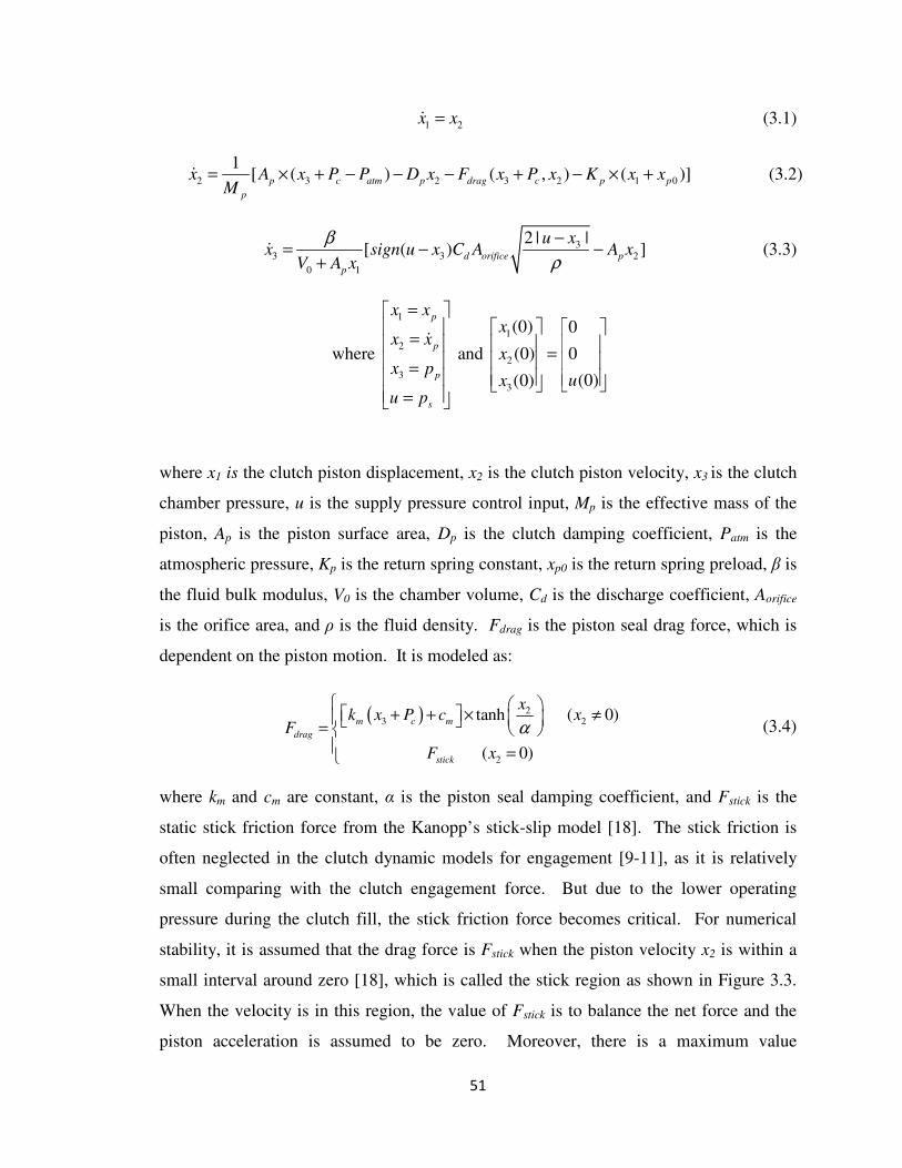
51

1 2x x=� (3.1)

2 3 2 3 2 1 0

1[ ( ) ( , ) ( )]p c atm p drag c p p

p

x A x P P D x F x P x K x xM

= × + − − − + − × +� (3.2)

33 3 2

0 1

2 | |[ ( ) ]d orifice p

p

u xx sign u x C A A x

V A x

β

ρ

−= − −

+� (3.3)

where

1

2

3

p

p

p

s

x x

x x

x p

u p

=

= = =

�

and

1

2

3

(0) 0

(0) 0

(0)(0)

x

x

ux

=

where x1 is the clutch piston displacement, x2 is the clutch piston velocity, x3 is the clutch

chamber pressure, u is the supply pressure control input, Mp is the effective mass of the

piston, Ap is the piston surface area, Dp is the clutch damping coefficient, Patm is the

atmospheric pressure, Kp is the return spring constant, xp0 is the return spring preload, β is

the fluid bulk modulus, V0 is the chamber volume, Cd is the discharge coefficient, Aorifice

is the orifice area, and ρ is the fluid density. Fdrag is the piston seal drag force, which is

dependent on the piston motion. It is modeled as:

( ) 23 2

2

tanh ( 0)

( 0)

m c m

drag

stick

xk x P c x

F

F x

α

+ + × ≠ = =

(3.4)

where km and cm are constant, α is the piston seal damping coefficient, and Fstick is the

static stick friction force from the Kanopp’s stick-slip model [18]. The stick friction is

often neglected in the clutch dynamic models for engagement [9-11], as it is relatively

small comparing with the clutch engagement force. But due to the lower operating

pressure during the clutch fill, the stick friction force becomes critical. For numerical

stability, it is assumed that the drag force is Fstick when the piston velocity x2 is within a

small interval around zero [18], which is called the stick region as shown in Figure 3.3.

When the velocity is in this region, the value of Fstick is to balance the net force and the

piston acceleration is assumed to be zero. Moreover, there is a maximum value

52

constraint for the stick friction. If the net force exceeds the maximum stick friction, the

piston will accelerate. The maximum stick friction, which is noted as Fstatic, is

proportional to the clutch chamber pressure and can be modeled as:

( )3static s c sF k x P c= + + (3.5)

where ks and cs are constant.

Fstatic

Fstick

Small interval

velocity x2

Figure 3.3. Stick friction diagram

In addition, Pc is the centrifugal force induced pressure generated from the rotation

of the clutch assembly [19]. The fluid pressure distribution Pct due to the centrifugal

force at any radius r can be expressed as:

( )222

2stct rrP −= ω

ρ (3.6)

where ω is the clutch system rotational speed and rst is the starting fluid level [20]. The

average fluid centrifugal pressure Pc on the effective piston area Ap can be expressed as:

2

po

pi

r

ct

r

c

p

P rdr

PA

π⋅

=

∫ (3.7)

where rpi and rpo are the piston inner and outer radius respectively.

53

3.2.2 Formulation of the Clutch Fill Control Problem

To enable a fast and precise clutch fill, the clutch piston must travel exactly the

distance d, which is required for the piston to contact the clutch pack, in the desired

clutch fill time T. Also, at time T, the piston velocity x2 should be zero, and the pressure

force inside the chamber must be equal to the spring force in order to keep the piston in

contact with the clutch pack. These requirements can translate into a set of final

conditions that the system must satisfy:

0

1 2 3

( )( ) , ( ) 0 ( )

p p

atm c

p

K d xx T d x T and x T P P

A

× += = = + − (3.8)

where d is the desired clutch stroke, and x1(T), x2(T) and x3(T) are the final states.

Among the controls that can bring the clutch from initial states to the final states (3.8),

we would like to take the one that has minimum peak flow demand. This will enable a

smaller displacement transmission pump, which in turn will improve the vehicle fuel

economy and reduce cost [8]. To reduce the peak flow demand, we need to minimize the

peak value of the piston velocity x2 during the clutch fill process since the clutch fill flow

is proportional to the piston velocity. Therefore, x2 should quickly approach the average

velocity, and stay at the average velocity as long as possible, and at the end goes to the

final state conditions as shown in Figure 3.4. Note that the total area enclosed by the x2

trajectory should be the piston displacement d.

x2 (m/s)

t (s)

Desired trajectory of x2

Piston velocity versus time

x2 (m/s)

t (s)


x2 (m/s)

t (s)


Piston velocity versus time

Figure 3.4. Desired trajectory of x2

54

In addition, the piston velocity can not increase too fast at the beginning of the clutch

fill. Before the clutch starts moving, the clutch chamber pressure increases and therefore

the stick friction on the clutch piston also increases. The stick friction will reach its

maximum value Fstatic and then the clutch piston will move. Once moving, the piston

drag force will switch from stick friction to drag force in motion, which is smaller than

the Fstatic. This friction force transient is non-smooth and nonlinear [18], which makes it

difficult to track and control a fast changing piston velocity profile given the fact that

currently there is no feedback sensor for the clutch fill process. Therefore, in Figure 3.5,

the initial velocity of the clutch fill is designed to be small for a short duration and then

rise quickly to its peak value.

However, the above considerations have not taken system robustness into account.

In particular, the solenoid valve, which is used to generate the input pressure command u,

has time delay and subsequently results in the shift of x2 trajectory as shown in Figure 3.5.

Note that the final time T is fixed, so the piston could not travel to the desired distance d

due to the shift and the difference between the desired trajectory and the shifted one will

be:

( )2

T

T T

d x t dt

−∆

∆ = ∫ (3.9)

Therefore, to minimize ∆d, the value of x2(t) between time T-∆T and T should be as

small as possible as shown in Figure 3.5, and we can claim that the unique trajectory of x2

will enhance the robustness of the system for time delay. In addition, from (3.8), we can

see that the clutch fill final states are determined by the spring stiffness Kp, the piston

area Ap, the spring preload xpo and the centrifugal pressure Pc. Kp, Ap, and xpo can be

measured accurately and will not change much with the environment. Pc can also be

accurately determined based on the transmission rotational speed, and it in fact has less

influence on the final condition due to its small magnitude comparing with the other

forces. Therefore the final states of the clutch fill system are quite robust.

55

x2 (m/s)

t (s)


TΔT

Shifted trajectory of x2

T20

T1

vm

Figure 3.5. Shifted trajectory of x2

Now we are ready to formulate the clutch fill control as an optimization problem.

The cost function of the optimization problem is:

1 2

1 2

2 2 2 2

2 1 2 2 2 3 1

0

02 2

4 2 5 3

[ ( ) ] [ ( ) ] [ ( ) ] [ ( ) ]

( )[ ( ) 0] { ( ) [ ]}

T T T

m m

T T

p p

atm c

p

dg x t v dt x t dt x t v dt x T d

T

K d xx T x T P P

A

λ λ λ

λ λ

= − + − + − + −

++ − + − + −

∫ ∫ ∫ (3.10)

In particular, the first term of the cost function ensures the piston to start with a low

velocity vm. The second term ensures that the velocity x2 remains close to the average

velocity d/T, which will minimize the peak value of x2 and therefore the peak flow

demand. The third term ensures x2 to be as small as possible (close to zero) from time T2

to final time T, which will enhance system robustness. The last three terms ensures that

the system will reach the specified final conditions in the required time T. λ1, λ2, λ3, λ4,

and λ5 are the weighting factors.

3.3. Optimal Control design

A systematic solution to the above optimization problem can be determined

recursively via Bellman’s Dynamic Programming. Since the system model (3.1-3.3) is

nonlinear, analytical solution cannot be obtained. Instead numerical solution will be

provided. But first we need to discretize the system model to carry out the numerical

Dynamic Programming method.

56

3.3.1 System Model Discretization

We discretize the system model (3.1-3.3) as follows:

( ) ( ) ( )1 2 11x k tx k x k+ = ∆ + (3.11)

( ) ( )

( )

2 2 3 2

3 2 1 0

( 1) ( ) { [ ]

, ( ) [ ( ) ]}

p c atm p

p

drag c p p

tx k x k A x k P P D x k

M

F x k P x k K x k x

∆+ = + + − − −

+ − × +

(3.12)

( )( )

( )( )

( ) ( )3

3 3 2 3

0 1

2 ( )1 { ( ) }

d orifice p

p

u k x ktx k sign u k x k C A A x k x k

V A x k

β

ρ

−∆+ = − × − + +

(3.13)

where ∆t refers to the sampling time interval. For presentation simplicity, define f as the

simple representation of the state space model (3.11-3.13), and define X(k)=[x1(k), x2(k),

x3(k)]T.

We define N=T/∆t as the number of steps from the initial state to the final state. And

the cost function (3.10) becomes:

1 2

1 2

12 2 2

2 1 2 2 2

0 1 1

02 2 2

3 1 4 2 5 3

( ) [ ( ) ] [ ( ) ] [ ( ) ]

( )[ ( ) ] [ ( ) 0] { ( ) [ ]}

N N N

m m

k k N k N

p p

atm c

p

dg X x k v t x k t x k v t

T

K d xx N d x N x N P P

A

λ λ

λ λ λ

−

= = + = +

= − ∆ + − ∆ + − ∆ +

+− + − + − + −

∑ ∑ ∑ (3.14)

Consequently, the optimal control problem is to find an optimal control input u to

minimize the cost function

( ) min ( )u U

J X g X∈

= (3.15)

where X=[X(0), ….. X(N)], u=[u(0),…., u(N)], and U represents the set of feasible control

inputs.

3.3.2 Applicability of Conventional Numerical Dynamic Programming to the

Optimal Clutch Fill Control

In this section, the applicability of conventional numeric Dynamic Programming for

57

the clutch fill control problem is explored. To convert the Dynamic Programming into a

finite computational problem, the standard method is to use state space quantization and

interpolation [12, 13, 16]. Though widely applied in numerical DP applications, the

conventional numerical DP algorithm is not suitable for solving the clutch fill control

problem. The system model (3.11-3.13) includes stiff dynamic equations [21], which is a

typical feature having the presence of rapidly changing transients [21]. The stiffness of

the system can be manifested mathematically by evaluating the Jacobian matrix of the

linearized form of the dynamic model (11-13) along its state trajectories [21]. This

stiffness feature will require DP to have a very high sampling rate. Typical ways to deal

with stiff dynamic equations like A-stable method [22] and newton’s iterative method are

not desirable in this application.

Besides, the conventional numerical Dynamic Programming also requires state space

discretization and interpolation, which also results in high computational burden. In

addition, the possible states for each step are discretized before the Dynamic

Programming process, but some of those are not reachable at all [16]. This is because the

system dynamics have already set constraints between x1(k), x2(k), x3 (k) and x1(k+1),

x2(k+1) and x3 (k+1), so the states can be reached only if they satisfy the specific dynamic

relationship. Consequently, certain quantified discrete states are actually not needed in

the Dynamic Programming process. Furthermore, the interpolation [16] used to calculate

the cost function will cause approximation errors. And the approximation errors will

propagate as the time step increases. It has been indicated that the interpolation error

tends to increase almost linearly [17].

3.3.3 Optimal Control Using a Customized Dynamic Programming Method

As shown above, the conventional numerical DP algorithm with interpolation is not

suitable to solve the clutch fill control problem. In this section, we present a customized

numerical Dynamic Programming method, which can generate an accurate optimal

control sequence with much reduced computational burden.

First, it is desirable to avoid the stiffness and sampling interval constraint associated

with the clutch fill dynamic model. One possible way to realize this is to have a proper

58

inversion of the model structure and therefore change its stiff characteristic. Given the

structure of the system model (11-13), if x1(k+1), x2(k+1), x3(k+1), and x2(k) are known,

we can calculate the values of x1(k), x3(k) and the input u(k) as follows:

( ) ( ) ( )1 1 2 11 ( )x k x k tx k R k= + − ∆ = (3.16)

( )3 2 ( )x k R k= (3.17)

( )2

3 3( ) ( )( ) ( )2

d orifice

Wu k sign W x k R k

C A

ρ= + = (3.18)

where

( ) ( )( )

( )0 1

3 3 2

[ ][ 1 ]

p

p

V A x kW x k x k A x k

tβ

+= + − × +

∆

The equation R2(k) determines the in-chamber pressure x3(k) in the step k and involves

the drag force Fdrag term, which has different models depending on the piston velocity x2.

When x2(k) is not zero, Fdrag can be obtained from equation (3.4) and R2(k) is:

( )( ) ( )

( ) ( )( )

2 2 2

2

2

2 1 0

1( ) {[ 1 ]

tanh[ ]

( ) [ ] ( ) tanh[ ]}

p

p m

p c atm p p p m m c

MR k x k x k

x k tA k

x kA P P D x k K x k x c k P

α

α

= × + − × −∆

− ×

− + + + + +

When x2(k) is zero but x2(k+1) is nonzero, which means that the piston starts moving, the

Fdrag is assumed to be the maximum static friction Fstatic in (3.5) and R2(k) becomes:

( ) ( )

( ) ( )

2 2 2

2 1 0

1( ) {[ 1 ]

( ) [ ] ( )}

p

p s

p c atm p p p s s c

MR k x k x k

A k t

A P P D x k K x k x c k P

= × + − × −− ∆

− + + + + +

When both x2(k) and x2(k+1) are zero, which means that the piston stays static, the

chamber pressure x3(k) variation is assumed to be small and R2(k) becomes:

2 3( ) ( 1)R k x k= +

For notation simplicity, we can denote Eq. (3.16), (3.17) and (3.18) as [x1(k), x3(k),

59

u(k)]=R[x1(k+1), x2(k+1), x3(k+1), x2(k)]. Note that as x2(k) is now predetermined in the

inverse dynamic model (3.16-3.18), it could be regarded as an input, and the new

unknown states become [x1(k), x3(k), u(k)]. Therefore, the Jacobian matrix of (3.16-3.18)

during clutch motion becomes:

1 2 3 2

1 3 1

3 3

1 3

1 0 0

[ ( ), ( ), ( )] ( )0 0

[ ( 1), ( 1), ( 1)] ( 1)

( ) ( )0

( 1) ( 1)

T

T

R k R k R k R k

x k x k u k x k

R k R k

x k x k

∂ ∂

= ∂ + + + ∂ +

∂ ∂

∂ + ∂ +

(3.19)

The eigenvalues of (19) are always inside or on the unit circle regardless of the

value of ∆t, which means the dynamic model (3.16-3.18) is not stiff [21] and therefore

the sampling interval constraint can be avoided. Note that the above model

transformation still requires the predetermined value for x1(k+1), x2(k+1), x3(k+1), and

x2(k). Interestingly, as the Dynamic Programming is implemented in a backward fashion,

x1(k+1), x2(k+1) and x3(k+1) were calculated in the previous step, and x2(k) can be

discretized into finite grids and predetermined in advance. Note that not all model

inversion will result in non-stiff dynamics. For example, the inverse model X(k)=

X(k+1)-f [X(k+1),u(k)] ×∆t ( f is the dynamic model (3.11-3.13)) using the backward

Euler method is still stiff [22].

Therefore, instead of making combinations of predetermined discrete values of x1(k),

x2(k) and x3(k) in the conventional DP [16], we only need to generate the predetermined

discrete values for x2(k) at each step, and then use the values of x1(k+1), x2(k+1), x3(k+1)

from previous step together with x2(k) to obtain the values for x1(k) and x3(k).

Consequently, unlike the conventional DP, which searches the entire quantified discrete

state space (the combinations of predetermined discrete grids) [16], the discrete states to

search are determined by the system dynamics (3.16-3.18), and therefore all the discrete

states searched in the DP computation are reachable.

However, although the discrete states generated by the above method are all

reachable, the number of discrete states will increase from step to step. Suppose the

60

number of discrete states at step k+1 is Lk+1, and the number of discrete values of x2(k) at

step k is L, then the total number of discrete states generated for step k would be

Lk=Lk+1×L. So the number of states will grow very quickly after N steps. To avoid this

problem, instead of discretizing the state space into specific discrete values, the

customized Dynamic Programming algorithm divides the state space into several regions.

As shown in Figure 3.6, {x20(k), x2

1(k),…x2

j(k)…x2

L(k)} are the discrete values of x2 at

step k, and {X0(k+1), X

1(k+1),…X

i(k+1),…X

Lk+1(k+1)} are the possible discrete states

calculated from step k+1. In addition, for each discrete value of x2(k), we can generate

several discrete regions on the plane of x1 and x3 shown as the black and white blocks in

Figure 3.6. Then suppose from

( ) ( )1 3 2[ , , ( )] [ ( 1), ( )]i i i i jx k x k u k R X k x k= + (3.20)

we get x1i(k) and x3

i(k), and suppose that [x1

i(k), x2

j(k), x3

i(k)]

T lies in region A in Figure

3.6. Subsequently, we can assign the vector [x1i(k), x2

j(k), x3

i(k)]

T as the value of region A,

and also memorize [x1i(k), x2

j(k), x3

i(k)]

T as one of the discrete states for step k. Moreover,

we can calculate the cost function based on [x1i(k), x2

j(k), x3

i(k)]

T as:

2

1 2 3 2 1

ˆ[ ( ), ( ), ( )] [ ( ) ] [ ( 1)]i j i j i

k e kJ x k x k x k x k v J X kλ

+= − + + (3.21)

where 1

ˆk

J+

is the cost function of state Xi(k+1) at step k+1. Here we also define two

symbols v and λe, which are equal to vm in (3.10) and 1 respectively when step k ≤ N1, are

equal to d/T and λ1 respectively when step k ≤ N2, and are equal to vm and λ2 respectively

when k > N2.

61

x1

x3

x2

x1

x1x3

x3

x20(k)

x2j(k)

…...

…...

x2L(k)

…...

…...

A

X0(k+1)

Xi(k+1)

Xi+c(k+1)

XLk+1(k+1)

x1

x3

x2

x1

x1x3

x3

x20(k)

x2j(k)

…...

…...

x2L(k)

…...

…...

A

X0(k+1)

Xi(k+1)

Xi+c(k+1)

XLk+1(k+1)

Figure 3.6. State space quantization

In the following calculation, if [x1i+c

(k), x2j(k), x3

i+c(k)]

T obtained from R[X

i+c(k+1),

x2j(k)] also lies in region A, we then calculate the cost function again based on [x1

i+c(k),

x2j(k), x3

i+c(k)]

T as:

2

1 2 3 2 1

ˆ[ ( ), ( ), ( )] [ ( ) ] [ ( 1)]i c j i c j i c

k e kJ x k x k x k x k v J X kλ+ + +

+= − + + (3.22)

If Jk[x1i(k), x2

j(k), x3

i(k)] is larger than Jk[x1

i+c(k), x2

j(k), x3

i+c(k)], we should reassign the

value of region A as [x1i+c

(k), x2j(k), x3

i+c(k)]

T, and at the same time [x1

i(k), x2

j(k), x3

i(k)]

T

in the discrete space will be replaced by [x1i+c

(k), x2j(k), x3

i+c(k)]

T. But if Jk[x1

i(k), x2

j(k),

x3i(k)] is smaller than Jk[x1

i+c(k), x2

j(k), x3

i+c(k)], [x1

i+c(k), x2

j(k), x3

i+c(k)]

T will be

disregarded and the process goes on.

We summarize the proposed customized Dynamic Programming algorithm as

follows:

First, x2(k) is discretized into a finite grid with size L, and the x1 and x3 plane

corresponding to each discrete x2j(k) is discretized into L×L regions.

1 2

2 2 2 2 2

1 2

( ) { ( ), ( ),..., ( ),..., ( )}

( ) { ( ), ( ),... ( ),..., ( )}

j L

h L L

j j j j j

x k x k x k x k x k

region k reg k reg k reg k reg k×

∈

∈ (3.23)

where regionj(k) refers to the discrete regions on x1--x3 plane corresponding to specific

x2j(k). Also define λ as a diagonal matrix whose diagonal elements are the weighting

62

factors λ3, λ4, λ5 in Eq (3.14).

Step N-1, for 1≤ j ≤ L,

( ) ( )1 3 2[ 1 , 1 , ( 1)] [ _ , ( 1)]jx N x N u N R X final x N− − − = − (3.24)

( ) ( )1 2 3( 1) [ 1 , ( 1), 1 ]j j

X N x N x N x N− = − − − (3.25)

2

1 2 2[ ( 1)] [ ( 1) ]

{ [ ( 1), ( 1)] } { [ ( 1), ( 1)] }

j j

N m

j T j

final final

J X N x N v

f X N u N X f X N u N X

λ

λ

−− = − − +

− − − − − − (3.26)

Step k, for 0≤ k <N-1, for 1≤ j ≤ L, and for 1≤ i ≤Lk+1

( ) ( )1 3 2[ , ( ), ] [ ( 1), ( )]i jx k x k u k R X k x k= + (3.27)

( ) ( )1 2 3[ , ( ), ]j

tempX x k x k x k= (3.28)

If ( )h

temp jX reg k∈ , then

2

_ 2 1[ ( ) ] [ ( 1)]

j i

k temp e kJ x k v J X kλ

+= − + + (3.29)

If _ 2

[ ( ), ( )]j h

k temp k jJ J x k reg k< , then

2 _[ ( ), ( )]

j h

k j k tempJ x k reg k J= (3.30)

( ) ( )1 2 3( ) [ , ( ), ]h j

j tempX k X x k x k x k= = (3.31)

Finally, after we have obtained the minimum cost function for each reachable state,

we can easily get the optimal sequence of control input u=[u(0),…., u(N)] which would

minimize the total cost function.

In summary, the proposed algorithm has three advantages over the conventional

numerical DP algorithm. First, the system dynamic model is transformed from stiff

equations into non-stiff equations. Thus, we can use a smaller number of steps (N=800 in

our simulation) for DP. Second, all the states in the process are reachable, so by getting

states x1(k) and x3(k) directly from x1(k+1), x2(k+1), x3(k+1) and x2(k) using Eq (3.20),

1ˆ

kJ + in (3.21) can be directly matched with Jk+1[x1(k+1), x2(k+1), x3(k+1)], therefore

eliminating the approximation errors caused by interpolation in the conventional

63

Dynamic Programming [16]. Third, as not all the discrete regions need to be considered

during the process, the curse of dimensionality [17] problem is mitigated.

3.4. Simulation and Experimental results

3.4.1 Experimental Setup

To validate the proposed optimal clutch fill control, a transmission clutch fixture is

designed and built as shown in Figure 3.7. The main parts include a servo motor, an

automotive transmission pump, a pilot-operated proportional relief valve, a proportional

reducing/relieving valve, two pressure sensors, a clutch mounting device/fixture, two

displacement sensors, a flow meter, a power supply unit with servo amplifier and an

XPC-target real time control system.

Power Supply Unit

with Servo Amplif ier

Displacement

Sensor

Clutch Fixture

PC with I/O

Terminal Boards

Pilot-Operated

Proportional

Relief Valve

Pressure

Sensors

Proportional

Reducing/

Relieving Valve

Pump Motor

Figure 3.7: Clutch fill experimental setup

The hydraulic circuit diagram is shown in Figure 3.8. A pump with a 2-stage pilot

operated relief valve provides the high pressure fluid. A servo amplifier unit controls the

speed of the pump motor. A proportional reducing/relieving valve is used to control the

fluid to the clutch chamber.

64

Pilot-Operated

Proportional Servo

Relief Valve

Displacement

Sensor

Pump Motor

Safety

Valve

Proportional

Reducing/Relieving

Valve

Clutch

Pressure

Sensors

I/O Board

PC

Figure 3.8. The hydraulic circuit scheme diagram

To measure the motion of the clutch fill process, the clutch system has been

instrumented with displacement, pressure and flow sensors. The clutch piston

displacement is measured by two different displacement sensors 180 degrees apart. A

micro gauging differential variable reluctance transducer (MGDVRT) is mounted on one

location of the clutch piston and a laser sensor is mounted 180 degree apart. Due to the

rubber sealing and manufacturing tolerance, the friction around the circular piston is not

necessarily balanced. This may cause the piston to twist around the shaft while moving.

Therefore it is necessary to measure the piston motion at different locations

simultaneously and calculate the average piston displacement. In addition, the clutch

system input pressure is measured using an Omega pressure sensor PX209-030G5V with

measurement range from 0 to 30 psi and the resolution of 0.075 psi, and a Max-

machinery flow meter G015 with the range from 0.15 to 15 lpm and the time constant of

1.7 ms is used to measure the input flow rate.

3.4.2. System identification

To implement the dynamic programming and optimal control, the parameters of the

clutch system model (1-3) need to be identified. The effective mass of the piston Mp, the

65

piston surface area Ap, the return spring constant Kp, the preload distance of the return

spring xp0, the stick friction peak value Fstatic, the orifice area Aorifice, the fluid density ρ,

the discharge coefficient Cd, the bulk modulus β and the clutch chamber volume V0 can

be measured or obtained directly. As the clutch is not rotating in the lab experimental

setup, the centrifugal pressure Pc is zero.

The Fstatic, which is the maximum drag force when the clutch stays static, is measured

by recording the clutch chamber pressure at the start of the piston motion. In the

experiment, the clutch piston is kept static at the specific travel distance and then moves

to the next position as shown in Figure 3.9. The minimum pressure Pmin required to

move the piston at the specified position is obtained as pointed by the arrow in Figure

3.9. Therefore Fstatic in the corresponding chamber pressure can be calculated by

min 1( )static p p po

F P A K x x= × − × + (3.32)

9 9.1 9.2 9.3 9.4 9.5 9.6 9.7 9.8 9.9 10-0.1

0

0.1

0.2

0.3

Time (s)

Dis

pla

cem

ent

(mm

)

9 9.1 9.2 9.3 9.4 9.5 9.6 9.7 9.8 9.9 101.5

1.6

1.7

1.8

1.9

2x 10

5

Time (s)

Pre

ssure

(P

a)

Figure 3.9. Experiments for measuring the stick friction Fstatic

66

0 0.5 1 1.5 2 2.5 31.2

1.4

1.6

1.8

2

time (second)

pre

ssure

(bar)

0 0.5 1 1.5 2 2.5 3-0.2

-0.1

0

0.1

0.2

time (second)

Modelin

g e

rror

(mm

)

(a) Input pressure profile. (b) Modeling error.

Figure 3.10. System identification model verification

The remaining model parameters, the damping coefficient Dp, the piston seal

damping coefficient α, and the piston seal drag force Fdrag while the piston is moving, are

identified using the least square estimation approach [23]. The identified model is then

compared with the experimental data using the input pressure profile shown in Figure

3.10(a), and the modeling error is shown in Figure 3.10 (b). Finally, the measured and

identified parameter values are presented in Table 3.1.

3.4.3. Clutch Fill Simulation and Experimental Results

In this section, both simulation and experimental results are reported to validate the

proposed control method. An optimal input pressure is derived to achieve the desired

clutch fill velocity profile using the customized dynamic programming method. The

desired final state conditions are x1(T)=d=0.000725 (m), x2(T) =0 (m/s), x3(T) =1.91 ×

105 (Pa). Figure 3.11 (solid red line) shows the optimal control input. The total steps for

DP is 800. The number of discrete values for x2(k) at each step is 100, and the number of

discrete regions for each discrete x2(k) value is 100×100. For the customized DP method,

we only evaluate the states that can be reached. The computation time for the customized

DP method is 22 minutes with a 1.86GHZ computer.

67

TABLE 3.1. PARAMETER VALUES OF THE SYSTEM DYNAMIC MODEL

Mp

xp0

Kp

Dp

Ap

α

V0

km

cm

0.4 (kg)

1.5928 (mm)

242640 (N/m)

135.4 (N/m/s)

0.00628 (m2)

4.1054e-6(m/s)

7.8e-5 (m3)

0.001517 (m2)

5.22 (N)

T

∆t

Aorifice

ρ

Cd

Patm

β

ks

cs

0.3 (s)

0.000375 (s)

2.0442e-5 (m2)

880 (kg/ m3)

0.7

1 (bar)

1625 (bar)

0.00153(m2)

5.26(N)

The resulting optimal control input pressure is then implemented in the experiment to

verify its performance as shown Figure 3.11 (dashed blue line). Due to the short time

duration (0.3 second) and total displacement (0.725 mm), precise pressure and motion

control of the clutch fill process is very challenging. In addition, the clutch mechanism is

extremely sensitive to pressure rise in the clutch chamber when the clutch piston starts to

move which adds up to the intricacy of controlling the clutch piston motion. This is

because the current clutch design behaves as an on/off switch during the clutch fill

process, where the input pressure required to start the piston motion is only 0.3 bar lower

than the final pressure (see Figure 3.11). Despite of these challenges, the clutch piston

displacement, velocity and the input flow profiles from the experiments exhibit optimal

shape as shown in Figure 3.12. The experimental velocity profile in Figure 3.12 (b) is

obtained by numerical differentiation of the displacement data, and its optimal shape can

be further verified by the smooth input flow rate shown in Figure 3.12 (c).

The repeatability issue is also verified using multiple experiments with the same

desired pressure inputs shown in Figure 3.11. The experimental results in Figure 3.13

exhibits good repeatability. Specifically, Figure 3.13 (a) presents the piston

displacements from five groups of experiments, which clearly show that all the

displacement trajectories have similar optimal shape and can overlap each other. Figure

3.13 (b) shows the error histogram of all the data points in the five trajectories comparing

68

with the desired one, which again exhibits good repeatability.

0 0.05 0.1 0.15 0.2 0.25 0.31.5

1.6

1.7

1.8

1.9

2

2.1

time (second)

pre

ssure

(bar)

Experimental pressure

Reference pressure from DP

Figure 3.11. Optimal input pressure and the experimental tracking results

0 0.05 0.1 0.15 0.2 0.25 0.30

0.2

0.4

0.6

0.8

(a) time (second)

Dis

pla

cem

ent

(mm

) Experimental

Simulated from DP

0 0.05 0.1 0.15 0.2 0.25 0.30

2

4

6

Velo

city (

mm

/s)

(b) time (seond)

0 0.05 0.1 0.15 0.2 0.25 0.30

1

2

3

4

5

(c) time (second)

flow

rate

(lp

m)

Figure 3.12. Experimental results for clutch displacement, velocity and input flow rate

69

0 0.05 0.1 0.15 0.2 0.25 0.3

0

0.2

0.4

0.6

0.8

(a) time(second)

dis

pla

cem

ent

(mm

)

exp 1

exp 2

exp 3

exp 4

exp 5

-0.25 -0.2 -0.15 -0.1 -0.05 0 0.05 0.1 0.15 0.2 0.250

20

40

60

(b) error(mm)

num

ber

of

tim

es

Figure 3.13. Clutch fill repeatability test (a). five groups of displacement profiles. (b)

histogram of data error comparing with optimal trajectory

0 0.05 0.1 0.15 0.2 0.25 0.30

0.2

0.4

0.6

0.8

time (second)

Dis

pla

cem

ent

(mm

)

+5% model error

-5% model error

+10% model error

-10% model error

(Piston displacement trajectories with 5% perturbation ( red solid line ), 10% parameter perturbation (black

dotted line),-5% parameter perturbation (green solid line), and -10% perturbation ( dashed purple line ).)

Figure 3.14. Clutch fill robustness test

-0.025 -0.02 -0.015 -0.01 -0.005 0 0.005 0.01 0.015 0.02 0.0250

2

4

6

8

10

piston final displacement (mm)

num

ber

of

tim

es

Figure 3.15. Histogram of clutch fill piston final position

We also added ±5% and ±10% perturbations to the dynamic model parameters (Dp, α,

β, Fdrag, ρ, Vo, Aorifice) and simulated the system performance using the designed control

70

input in Figure 3.11. The trajectories shown in Figure 3.14 arrived in acceptable intervals

around the desired final states and thus demonstrated system robustness against those

model parameter variations. In addition, random perturbations within ±10% interval are

also added to those model parameters, and the resulted piston final displacements at the

end of the clutch fill are collected through 100 tests. The clutch fill final piston position

errors are then projected into a histogram shown in Figure 3.15. The histogram shows

that most of the clutch trajectories finally arrive within a small interval around 0.725mm,

which is the desired displacement of the clutch fill.

The influence of the time delay caused by the solenoid valve was explored as well.

The desired optimal clutch fill piston displacement is compared to that with solenoid

valve delay in Figure 3.16. Because of the unique velocity profile proposed in Figure 3.5,

the clutch fill with solenoid delay can still reach the final position within the required

clutch fill duration (0.3 second).

0 0.05 0.1 0.15 0.2 0.25 0.30

0.2

0.4

0.6

0.8

time(second)

dis

pla

cem

ent

(mm

)

Desired optimal displacement

delayed displacement profile

Figure 3.16. Experimental data demonstrating clutch fill robustness on time delay

Comparison with a non-optimal clutch fill process is also shown in Figure 3.17. It

can be seen that the non-optimal approach results in a high clutch piston velocity spike,

which represent the high peak flow demand that could only be met with a larger and less

fuel efficient pump.

71

0 0.05 0.1 0.15 0.2 0.25 0.3

0

5

10

15

20

25

30

time (second)

velo

city (

mm

/s)

Optimal clutch fill

Non-optimal clutch fill

Figure 3.17. Optimal and non-optimal clutch fill velocities profile comparison

3.5. Conclusion

This chapter presents a systematic approach for transmission clutch fill control using

a new customized Dynamic Programming method. The objective of the clutch fill

control is to enable a fast and precise clutch fill and reduce the peak flow demand. We

formulated this problem into a constrained optimization problem. To reduce the

computational burden and eliminate the interpolation errors in the conventional numerical

DP method, a customized Dynamic Programming method was proposed. The

customized DP algorithm transforms the original stiff system dynamic model to a non-

stiff one and thus avoids the large number of steps required by the sampling time of the

discretized clutch model. Furthermore, comparing with the conventional DP, it is free of

interpolation error and reduces the computational burden by selectively searching the

reachable states. To validate the optimal control, a transmission clutch fixture is

designed and built for experimental investigation. A dynamic model that captures the key

clutch fill dynamics is constructed and identified with the experimental data. Finally,

simulation and experimental results show the effectiveness of the proposed control

method.

72



Configurations in Passenger Cars”. SAE Technical Paper 2001-01-0882.




[3] Sun, Z. and Kumar, H., “Challenges and opportunities in automotive transmission

control”. Proceedings of 2005 American Control Conference, Portland, OR, USA,

June 8-10, 2005.







Transmission Control Strategy”. SAE Technical Paper 2007-01-1313

[7] Han, W. and Yi, S.J., “A Study of Shift Control Using the Clutch Pressure Pattern in

Automatic Transmission.” Proc. Instn Mech. Engrs Part D: Journal of Automobile

Engineering. Volume 217, Number 4/2003, pp 289-298

[8] Miao, H., Sun, Z., Fair, J., Lehrmann, J., Harbin, S. “Modeling and Analysis of the

Hydraulic System for Oil Budget in an Automotive Transmission”. Proceedings of

ASME 2008 Dynamic Systems and Control Conference, Ann Arbor, Michigan, USA,

October 20-22, 2008

[9] Montanari, M., Ronchi, F., Rossi, C., Tilli, A., Tonielli, A., “Control and

Performance Evaluation of a Clutch Servo System With Hydraulic Actuation”,

Journal of Control Engineering Practice, Vol. 12, Issue 11, pp. 1369-1379, Nov, 2004

73

[10] Horn, J., Bamberger, J., Michau, P., Pindl, S., “Flatness-based Clutch Control for

Automated Manual Transmissions”, Journal of Control Engineering Practice, Vol. 11,

Issue 12, pp. 1353-1359, Dec, 2003

[11] Glielmo, L., Iannelli, L., Vacca, V., “Gearshift Control for Automated Manual

Transmissions”, IEEE/ASME Transactions on Mechatronics, Vol. 11, No.1, pp. 17-

26, Feb., 2006.

[12] Bellman, R. E. (1957). Dynamic programming. Princeton University Press, New

Jersey.

[13] Bellman, R. E. and Dreyfus, S. E. (1962). Applied dynamic programming. Princeton


[14] I. Kolamanovsky, I. Siverguina, and B. Lygoe, “Optimization of Powertrain

Operating Policy for Feasibility Assessment and Calibration: Stochastic Dynamic

Programming Approach,” Proceedings of the American Control Conference,

Anchorage, AK, pp 1425-1430, May 8-10, 2002

[15] Daekyun Kim, Huei Peng, Shushan Bai, and Joel M. Maguire. “Control of Integrated

Powertrain with Electronic Throttle and Automatic Transmission.” IEEE

Transactions on Control Systems Technology, Vol. 15, Issue 3, pp. 474 – 482, May

2007

[16] J.M. Kang, I. Kolmanovsky and J.W. Grizzle, “Dynamic Optimization of Lean Burn

Engine Aftertreatment.” ASME Transactions on Journal of Dynamic Systems,

Measurement, and Control, Vol. 123/153, pp. 153-160, June 2001

[17] De Madrid, A.P. Dormido, S., and Morilla, F., “Reduction of the Dimensionality of

Dynamic Programming: A Case Study,” Pro. Of 1999 American Control Conference,

pp 2852-2856, June 1999

[18] Karnopp, D., “Computer Simulation of Stick-Slip Friction in Mechanical Dynamic

Systems”, ASME Transactions on Journal of Dynamic Systems, Measurement, and

Control, Vol. 107, No. 1, pp. 100-103, March 1985

[19] Song, X., Zulkefli, A., Sun, Z. and Miao, H., “Modeling, Analysis, and Optimal

Design of the Automotive Transmission Ball Capsule System”, ASME Transactions

74

on Journal of Dynamic Systems, Measurement and Control, Vol. 132, 021003,

March, 2010.

[20] Song, X., Sun, Z., Yang, X., Zhu, G., “Modeling, Control and Hardware-in-the-Loop

Simulation of an Automated Manual Transmission”, Proc. Instn Mech. Engrs Part D:

Journal of Automobile Engineering, Vol. 224, No. 2, pp.143-160, 2010.

[21] Hairer, E., Wanner, G., 1996. Solving Ordinary Differential Equations II (second

edition), Springer Series in Computational Mathematics

[22] Gautschi, W., 1997. Numerical Analysis: An Introduction, Birkhauser Boston

[23] Crassidis, J.L. and Junkins, J.L. “Optimal Estimation of Dynamic Systems”.

Chapman and Hall/CRC Applied Mathematics and Nonlinear Science Series, CRC

Express LLC, 2004.

75

NOMENCLATURE IN CHAPTER 3

C35R: clutch corresponding to gear ratio 3, 5, and reverse gear.

CB26: clutch corresponding to gear ratio 2 and 6.

CB1R: clutch corresponding to gear 1 and reverse gear.

C1234: clutch corresponding to gear 1, 2,3 and 4.

C456: clutch corresponding to gear 4, 5, and 6.

S1, S2, S3: sun gear in the planetary gear set.

R3, R12: ring gear in the planetary gear set.

ps: supply pressure

pp: pressure inside the clutch chamber

xp: clutch piston displacement

u: input pressure, = ps

x1: state, clutch piston displacement, = xp

x2: state, clutch piston velocity

x3: state, pressure inside the clutch chamber, = pp

X: =[x1(k), x2(k), x3(k)]T

X_final: clutch fill final states

Mp: effective mass of the piston

Ap: piston surface area

Dp: clutch damping coefficient

Patm: atmosphere pressure

Kp: return spring constant

xp0: return spring preload

β: the fluid bulk modulus

V0 : the clutch chamber volume

Cd: discharge coefficient

76

Aorifice: the orifice area

ρ: the fluid density

Fdrag is the piston seal drag force

km: drag force equation constant

cm: drag force equation constant

ks: static friction equation constant

cs: static friction equation constant

α : the piston seal damping coefficient

Fstick : the static stick friction force

Fstatic : maximum stick friction

Pc: centrifugal pressure

rpi and rpo : the piston inner and outer radius respectively

d: desired clutch stroke

∆T: valve time delay

T: final time

λ1, λ2, λ3, λ4, and λ5 : the weighting factors for cost function

v & λe: two symbols defined under Eq (21).

N: number of steps in dynamic programming

g: total cost function

J: minimized cost function

vm: a reference low velocity in Eq (10)

f: discrete state space model

R: customized DP transformation function.

reg: customized DP discretized region.

L: number of discretized values for a single state in DP

∆t: discrete dynamics time step interval

77

Chapter 4

The Clutch Level Design-- Pressure Based Closed Loop Clutch

Control

Both Chapters 1 and 2 investigate the clutch control approaches in an open loop

fashion. This is a viable solution in most of the current automatic transmission clutch

systems due to cost and compactness concern. With the increasing demand of

transmission efficiency and performance, and also to enable aggressive mode shifts for

multi-mode hybrid transmission, a more precise clutch shift control is necessary, which

calls for the closed loop clutch control. This chapter will be devoted to exploring the

possible robust clutch control means based on potential feedback sensors.

4.1 Introduction

With the increasing demand for fuel efficiency and reduced emissions, new

technologies have emerged in the automotive transmission systems [1-3]. Clutch to

clutch shift control [3-7] is a key enabler for fuel efficient, compact and low cost

transmission designs, including automatic transmissions [3], dual clutch transmissions

[8], and hybrid transmissions [9-11]. Specifically, Figure 1(a) shows a simplified

schematic diagram of a six speed automatic transmission [2], with five sets of clutch

packs and three planetary gear sets. During the gear shift, one clutch (on-coming clutch)

needs to be engaged while another (off-going clutch) needs to be disengaged [2]. This

process is called clutch-to-clutch shift [4-7]. For a smooth clutch-to-clutch shift, proper

control of two consecutive processes is necessary. First, precise coordination of the on-

coming clutch and off-going clutch is critical, which otherwise will cause undesirable

torque interruption and oscillations [3]. To ensure precise synchronization, before clutch

engagement, it is necessary to fill the oncoming clutch to a position where the clutch

packs are just in contact. This process is called clutch fill. Second, during the clutch

engagement process, which typically occurs right after the clutch fill, smooth and precise

torque control is crucial.

78

(a). Scheme diagram of a six speed automatic transmission

Fluid Inlet

Piston

Clutch Chamber

Orifice

Rotational axis

(center of shaft )

Clutch Pack

Spring

Fluid Inlet

Piston

Clutch Chamber

Orifice

Rotational axis

(center of shaft )

Clutch Pack

Spring

ball capsule valve

(b). Clutch actuation mechanism

0 1 2 3 4 5 6 7 8 950

100

150

200

250

Clu

tch T

orq

ue (

New

ton.m

)

Clutch Displacement(mm)

Wet clutch Dry clutch

(c). Schematic clutch characteristic curves for dry and wet clutches

Fig. 4.1. Clutch system diagrams

79

The commonly used clutch actuation device in transmissions is an electro-hydraulically

actuated clutch. Figure 4.1(b) shows a schematic diagram of a typical transmission clutch

actuation system. When the clutch is to be engaged, pressurized fluid will flow into the

clutch chamber and pushes the clutch piston forward until they are in contact (clutch fill).

At the end of the clutch fill, the input pressure is further increased, which then squeezes

the clutch piston to the clutch packs. It is important to control the clutch piston to reach

the clutch packs within a specified time because an improper clutch fill can cause the

failure of the clutch shift synchronization and then affect shift quality.

In this chapter, we will specifically study the hydraulically actuated “wet” clutch,

which is widely applied in the planetary gear automatic transmissions [3] and hybrid

transmissions [9-11]. This attributes mainly to the high power density of electro-

hydraulic systems and the heat dissipation ability of “wet” clutches. The control of “wet”

clutches is unique comparing with its counterpart “dry” clutch, which will be further

analyzed in the following paragraphs. Currently there is no pressure sensor inside the

clutch chamber, and therefore the clutch control in the automatic transmissions is either

in an open loop fashion or controlled using speed signal as the feedback. However, the

speed signal can only be used as the feedback variable during the clutch engagement, but

not for the clutch fill. With the increasing demand of transmission efficiency and

performance, a more precise clutch shift control is necessary, which calls for a more

effective closed loop clutch control. There are two possible ways of measuring the clutch

motion directly: by measuring the clutch piston displacement or measuring the pressure

inside the clutch chamber. In this chapter, the pressure feedback is selected for “wet”

clutch control due to three reasons. First, although the transferred torque can be

calculated from the clutch pack displacement, the displacement vs torque curve for “wet”

clutch is very steep comparing with “dry” clutch [12,27] as shown in Figure 4.1(c), which

makes it difficult to obtain an accurate torque estimate from the displacement. In

contrast, the pressure based information can be directly related to the transferred torque

during the clutch engagement. Second, with a compact transmission design, it is very

difficult to package a displacement sensor that moves with the clutch piston. Third, for

the wet clutch used in automatic transmissions, the total displacement of the clutch piston

80

is about 1~2 mm, and a high resolution displacement sensor for such a small range is

usually cost prohibitive for mass production.

Previous research works [12-15] on clutch control mainly focus on the “dry” clutch

engagement control, which has a longer clutch piston stroke comparing with the “wet”

clutch. Reference [12] introduces the automated manual transmission control with a PID

controller. Ref [13] presents a switching approach between a local controller and a global

controller with a pneumatic actuator and an on/off valve. Ref [14] considers dry clutch

engagement position tracking problem using dynamics inversion and backstepping. In

reference [15], a flatness based displacement tracking controller is designed for

automated manual transmission dry clutch engagement based on the fact that the relative

degree of its nonlinear system is equal to the system order. Although showing promising

results, approaches used in [12-15] focus on engagement control and all require

displacement feedback, and therefore cannot be directly applied to wet clutch fill and

engagement control. In addition, reference [16] presents an H-infinity control design for

regulating clutch rotational slipping speed and its implementation with a virtual clutch

model. Reference [17] and [18] report the backstepping design and a reduced order

nonlinear observer respectively for the clutch slipping control using the clutch rotational

speed as the feedback signal. Both references [17] and [18] report interesting simulation

results. However, slip speed feedback [16-18] cannot be used for the clutch fill phase, and

it is not a direct feedback on the transferred torque comparing with the pressure feedback.

This chapter focuses on pressure based control for the clutch fill and engagement of

“wet” clutch packs in automatic or hybrid transmissions. Comparing with the intensively

researched “dry” clutch displacement based engagement control [12-15], this control has

several challenges. First, the “wet” clutch system has a much shorter stroke, which

demands for very precise position and pressure (torque) control. On the one hand, the

dynamics modeling from the beginning of the clutch fill (low pressure) to the end of the

clutch engagement (intermediate to high pressure) covers a wider pressure range, which

results in several unique dynamic phenomena. On the other hand, the clutch fill process

has a very short stroke and it demonstrates an on/off behavior, where the activating

pressure is very close to the final pressure. With a small difference in pressure range and

less than 1 mm of clutch piston travel, precise control of the piston motion to avoid either

81

“over-fill” or “under-fill” [3] becomes very challenging. Second, the modeled system

dynamics are highly nonlinear with a single relative degree and second order internal

dynamics, and applying a systematic nonlinear robust control to achieve precise pressure

tracking is challenging. Although the sliding mode control is a potential candidate for the

robust control design with this specific dynamic structure, its chattering effect due to high

gain is still troublesome in reality. Therefore a systematic approach to design the gain for

this application is necessary. Third, only measuring the pressure without the piston

displacement makes the control difficult. On the one hand, it is hard to diagnose the

clutch fill process, which usually requires the piston position data. On the other hand, a

higher sliding mode gain is necessary due to the lack of the internal dynamics state

information (piston displacement and velocity), as otherwise a dynamic loading variation

caused by the start of the piston motion will result in a sudden pressure drop and

subsequently the pressure tracking failure during this transient. Clearly an appropriate

method of estimating the piston motion is required.

To address the above challenges, this chapter presents a systematic approach for

modeling and controlling of wet clutches with pressure feedback. First, the system

dynamic model is explored. Specifically, the proportional pressure reducing valve

dynamics, the mechanical actuator dynamics, and the wet clutch pressure dynamics are

constructed and validated with extensive experiments. Several unique phenomena are

revealed for the system dynamics. Due to the wide range of pressure change, variation of

the bulk modulus is critical. Due to the design of the clutch piston assembly, it is

observed that the clutch piston may twist around the shaft, which presents a challenge for

measuring the piston displacement at one location. This observation is critical for the

dynamics modeling to decide the start of the piston motion. Second, a sliding mode

controller is designed to regulate the clutch chamber pressure. To avoid the chattering

effect, precise and less conservative estimation of the system unmodeled dynamics is

crucial. This can be obtained from the experimental data in the first step. The gain of the

sliding mode control is then designed based on the bounds of the unmodeled dynamics to

ensure robust tracking while avoid chattering. Finally, an observer for piston motion is

built based on the pressure measurement. The piston displacement and velocity

estimation is not only a necessary compensation term to alleviate the sliding mode

82

controller high gain demand, but also a diagnosis tool for detecting the start and end of

the clutch fill process.

To validate the proposed modeling and control approach, a transmission clutch fixture

and hydraulic control circuit are designed and built. Through a series of experiments, the

dynamic model parameters are identified. To this end, the robust pressure controller and

observer are designed and implemented. Experimental results show the precise tracking

performance of the clutch chamber pressure, as well as comparisons with various control

configurations.

The rest of the chapter is organized as follows. Section 4.2 presents the system

dynamics modeling. Section 4.3 presents the sliding mode based nonlinear control and

the observer design. Section 4.4 describes the experimental system setup and the dynamic

model identification. Experimental results demonstrating the control performance are

shown in section 4.5. Conclusion is provided in section 4.6.

4.2 System Dynamics Modeling

Figure 4.2 shows a simplified schematic diagram of the clutch actuation system. The

main components include a pump, hydraulic control valves, a clutch assembly, pressure

and displacement sensors. The proportional pressure reducing valve controls the flow in

and out of the clutch chamber. When the clutch fill begins, the valve will connect the

clutch chamber to the high pressure source, which is regulated by a relief valve, and the

high pressure fluid flows into the chamber and pushes the piston towards the clutch pack.

Once the clutch fill ends, the valve will control the chamber pressure to further increase

until the clutch packs are fully engaged. When the clutch is disengaged, the proportional

pressure reducing valve connects the clutch chamber to the tank, and the clutch return

spring pushes the clutch piston back to the disengaged position. The clutch dynamic

model consists of the valve dynamics, the clutch mechanical actuator dynamics, and the

clutch chamber pressure dynamics, which will be presented in the following sessions.

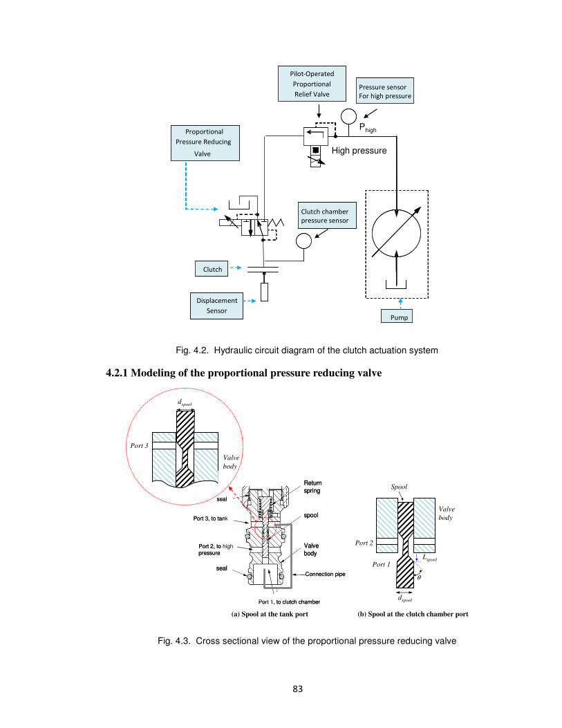
83

Pilot-Operated

Proportional

Relief Valve

Displacement

SensorPump

Proportional

Pressure Reducing

Valve

Clutch

High pressure

Phigh

Pressure sensor

For high pressure

Clutch chamber

pressure sensor

Fig. 4.2. Hydraulic circuit diagram of the clutch actuation system

4.2.1 Modeling of the proportional pressure reducing valve

Lspool

dspool

Port 2

Port 1

Spool

Valve

body

(a) Spool at the tank port (b) Spool at the clutch chamber port

dspool

Port 3

Port 1

Valve

body

Return spring

spool

Valve body

seal

Port 1, to clutch chamber

Port 3, to tank

Port 2, to high pressure

Connection pipe

seal

Return spring

spool

Valve body

seal

Port 1, to clutch chamber

Port 3, to tank

Port 2, to high pressure

Connection pipe

seal

θ

Fig. 4.3. Cross sectional view of the proportional pressure reducing valve

84

The valve used to control the clutch chamber pressure is a three way two position

proportional pressure reducing valve. Figure 4.3 (a) shows its cross section. Port 1 is

connected to the clutch chamber with pressure Pr, port 2 is connected to the supply

pressure Phigh, and port 3 is connected to the tank. The orifice between the clutch

chamber (port 1) and the supply pressure (port 2) is determined by the spool position,

which is controlled by the input voltage.

When there is no control voltage, the spool is kept at the top position by the return

spring. At this position port 3 is connected to port 1. Therefore the fluid inside the clutch

chamber will flow to the tank. When a positive voltage is exerted on the magnetic coil,

the induced magnetic force will push the spool towards port 1. As the spool connects

port 1 to port 2, the high pressure fluid will flow into the clutch chamber. The increased

pressure in port 1 will push the spool upward and eventually close the orifice between

port 1and port 2. Clearly, the spool position is determined by the magnetic force Fmag,

the returning spring force Fspring, and the chamber pressure Pr.

The spool dynamics can be described as:

1[ ( ) ( )

]

spool spool

spool mag spring spool pre load

spool

spool spool spool r

L v

v F Vol K L LM

D v A P

−

=

= − +

− −

�

� (4.1)

where max minmin

max

( ) ( )mag f f

i iF Vol K i K Vol i

Vol

−= × = × + (4.2)

Lspool is the spool position, vspool is the spool velocity, Mspool is the spool mass, Kspring is

the spool spring constant, Aspool is the cross sectional area of the spool, and Dspool is the

damping coefficient. Lpre-load is the spool position where the orifice between port 1 and

port 2 is just closed. Fmag is the magnetic force, which is determined by the coil magnetic

constant Kf and the current i. The current i is generated by the power amplifier and can

be calculated using the input voltage Vol. imax and imin are the maximum and minimum

current that can be generated from the power amplifier, and Volmax is the maximum

control voltage corresponding to imax.

85

As shown in Figure 4.3 (b), given the spool position Lspool, the orifice area Aorifice

between the high pressure port 2 and chamber pressure port 1 is:

( )( ) sin( ) sin cosorifice spool spool spool spool

A L L d Lπ θ θ θ= × − (4.3)

where dspool is the diameter of the spool, and θ is the spool surface slant angle as shown

in Figure 3(b).

Similarly, as shown in Figure 4.3 (a), the orifice area Adump between the tank port 3 and

the pressure port 1 is:

( )( ) sin( ) sin cosdump spool spool spool spool

A L L d Lπ θ θ θ= − × + (4.4)

Then the flow dynamics across the valve orifice is:

2( ) ( ) ,

0

( , ) 0 , 0

2( ) , 0

h r

h r d orifice spool

spool

spool r spool

r

d dump spool spool

P Psign P P C A L

L

Q L P L

PC A L L

ρ

ρ

−−

>

= = − <

(4.5)

where ρ is the fluid density, Cd is the discharge coefficient, Aorifice is the orifice area

connecting the clutch chamber (port 1) and the supply pressure (port 2), and Adump is the

orifice area connecting the clutch chamber (port 1) and the tank (port 3). When the spool

position Lspool > 0, the clutch chamber is connected to the high pressure. When the spool

position Lspool < 0, the clutch chamber is connected to the tank.

4.2.2 Mechanical System Modeling

The dynamics of clutch motion can be modeled as [20]:

1 2x x=� (4.6)

86

2 2

2 1 0

1[ ( )

( , ) ( )]

p r c atm p

p

drag r c res p

x A P P P D xM

F P P x F x x

= × × + − −

− + − +

�

(4.7)

where x1 is the clutch piston displacement, x2 is the clutch piston velocity, Mp is the

effective mass of the piston, Ap is the piston surface area, Dp is the clutch damping

coefficient, Patm is the atmospheric pressure, xp0 is the return spring preload. Pc is the

centrifugal force [21,22] induced pressure generated from the rotation of the clutch

assembly.

Fres is the displacement dependent resistance force. During the clutch fill, the

resistance force comes from the return spring, thus the force Fres depends on the spring

stiffness constant Kcs. During the clutch engagement, the resistance force is due to the

squeezing of the clutch pack, and therefore, the resistance force Fres can be modeled as:

1 0 1

1 0 1

( ) ( )

( ) ( )

cs p fill

res

en p fill

K x x x xF

F x x x x

× + ≤=

+ > (4.8)

where the function Fen(x1+xp0) include both spring force and the nonlinear clutch pack

reaction force, xfill is the clutch piston position at the end of the clutch fill.

Fdrag is the piston seal drag force, which is dependent on the piston motion. It is

modeled as:

( ) ( )2 2

2

( 0)

( 0)

m r c m

drag

stick

k P P c sign x xF

F x

+ + × ≠ = =

(4.9)

where km and cm are constant, and Fstick is the static stick friction force from the

Kanopp’s stick-slip model [23]. Further detail of the mechanical dynamic model can be

found in our recent work [20].

4.2.3 Modeling of the clutch chamber pressure dynamics

When the orifice between the high pressure port and the clutch chamber is open, the

fluid will flow into the clutch chamber, which results in the pressure rise in the chamber.

The pressure dynamics is modeled as:

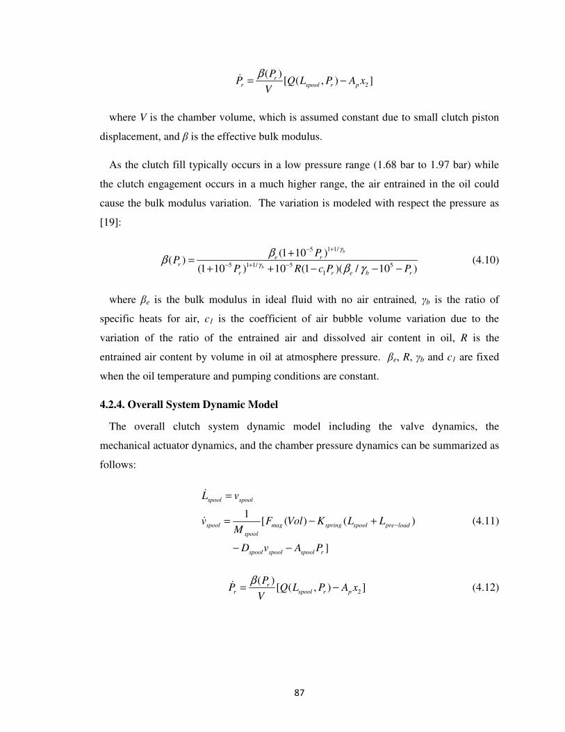
87

2

( )[ ( , ) ]r

r spool r p

PP Q L P A x

V

β= −�

where V is the chamber volume, which is assumed constant due to small clutch piston

displacement, and β is the effective bulk modulus.

As the clutch fill typically occurs in a low pressure range (1.68 bar to 1.97 bar) while

the clutch engagement occurs in a much higher range, the air entrained in the oil could

cause the bulk modulus variation. The variation is modeled with respect the pressure as

[19]:

1 1/5

1 1/5 5 5

1

(1 10 )( )

(1 10 ) 10 (1 )( / 10 )

b

b

e r

r

r r e b r

PP

P R c P P

γ

γ

ββ

β γ

+−

+− −

+=

+ + − − − (4.10)

where βe is the bulk modulus in ideal fluid with no air entrained, γb is the ratio of

specific heats for air, c1 is the coefficient of air bubble volume variation due to the

variation of the ratio of the entrained air and dissolved air content in oil, R is the

entrained air content by volume in oil at atmosphere pressure. βe, R, γb and c1 are fixed

when the oil temperature and pumping conditions are constant.

4.2.4. Overall System Dynamic Model

The overall clutch system dynamic model including the valve dynamics, the

mechanical actuator dynamics, and the chamber pressure dynamics can be summarized as

follows:

1[ ( ) ( )

]

spool spool

spool mag spring spool pre load

spool

spool spool spool r

L v

v F Vol K L LM

D v A P

−

=

= − +

− −

�

� (4.11)

2

( )[ ( , ) ]r

r spool r p

PP Q L P A x

V

β= −� (4.12)

88

1 2x x=� (4.13)

2 2

2 1 0

1[ ( )

( , ) ( )]

p r c atm p

p

drag r c res p

x A P P P D xM

F P P x F x x

= × × + − −

− + − +

�

(4.14)

Further investigation reveals that the time constant of the pressure reducing valve is far

less than the time constant of the clutch actuation system pressure dynamics, which

means that the dynamic behavior of the reducing valve can be neglected. This fact can be

well exhibited from the experimental data shown in Figure 4.10(a) and (c). A step

voltage is applied to the valve at 0.07 second. On the one hand, Figure 4.10 (c) shows the

measurement of the flow rate through the valve opening orifice. Once the step signal is

on, the valve quickly opens to its full orifice, which is reflected from the near step jump

of the flow rate measurement close to 0.08 second and indicate that the valve time

constant is around 10 ms. On the other hand, Figure 4.10(a) shows the pressure dynamics

profile inside the clutch chamber. With a near step flow rate input shown in Figure

4.10(c), the pressure inside the clutch chamber slowly increases to its peak value in

almost 0.4 second, which indicates the time constant to be around 320 ms in this case.

This slow response is partially due to a low bulk modulus value at the low pressure.

Therefore, to simplify the control design, the proportional valve spool dynamics is

converted into a static mapping,

1[ ( ) ]spool mag spring pre load spool r

spring

L F u K L A PK

−= − × − (4.15)

Here, we denote u =Vol as the control input to the proportional valve.

Therefore, the system dynamics (4.11-4.12) becomes:

2

( )[ ( , ) ]r

r r p

PP Q u P A x

V

β= −� (4.16)

89

where

2( ) ( ) ,

( , ) 0

( , ) 0 , ( , ) 0

2( ) , ( , ) 0

h r

h r d orifice spool

spool r

r spool r

r

d dump spool spool r

P Psign P P C A L

L u P

Q u P L u P

PC A L L u P

ρ

ρ

−−

>

= = − <

(4.17)

Finally the reduced order system dynamics include Eqs (4.13) - (4.17).

In addition, for a given flow rate q, the required control input u can also be determined

based on Eqs (4.3), (4.4), (4.15) and (4.17). This relationship will be used in the next

section and the mapping from q to u can be written as:

maxmin

max min

( , )

( )

r

spool spring spring pre load spool r

f

U q P

L K K L A PVoli

i i K

−

=

+ +× −

−

(4.18)

where

2

2

4 cos( )

2( )

, 0sin(2 )

0 , 0

4 cos( )

2

, 0sin(2 )

spool spool

h r

h r d

spool

spool spool

r

d

qd d

P Psign P P C

q

L q

qd d

PC

q

θ

πρ

θ

θ

πρ

θ

− −

− − >

= = − + +

<

(4.19)

Eq. (4.19) is to calculate the spool position Lspool corresponding to a specific valve

opening orifice based on Eq. (4.3) and Eq. (4.4). The relationship between equation

(4.17) and (4.18) can be written as Q{ U (q, Pr ), Pr }= q.

90

4.3. Robust Nonlinear Controller and Observer Design

4.3.1. Sliding Mode Controller Design for Pressure Control

The clutch system (4.13-4.17) is a third order nonlinear system. As both the control

input u (the valve voltage) and the control output Pr (the chamber pressure) appear in the

dynamic equation (4.16), the system has a nonlinear dynamics with relative degree 1 [24].

Eq. (4.13) and (4.14) are the system internal dynamics, the equilibrium point of which is

asymptotically stable (The proof is straightforward, thus is omitted here). Therefore the

nonlinear system is minimum phase [24]. Note that the internal dynamics in this

application is a spring mass damper system, therefore the minimum phase feature also

suggests that the whole system will be stabilized as long as the states other than the

internal dynamics states could be stabilized. This unique feature suggests applying the

sliding mode controller, which can ensure system robustness with a relatively low order

controller design [24].

Define the tracking error e2 as the difference between the desired pressure trajectory r

and the actual measurement Pr.

2 re P r= − (4.20)

And define another error term e1, the derivative of which is equal to e2.

1 2e e=� (4.21)

With the pressure dynamics in (4.16), we have

2

2 2 1

2 1 2

( )[ ( , ) ( , ) ] ( )

( ) ( ) ( )( , ) ( ) ( , )

r

r

r r p r

r r r

r p r r

e P r

PQ u P u P A x P r

V

P P PQ u P A x r P u P

V V V

β

β β β

= −

= + ∆ − + ∆ −

= − − + ∆ + ∆

��

�

�

(4.22)

where ∆1(Pr) represents the model uncertainty of the pressure dynamics (4.16), and

∆2(u, Pr) represents the model uncertainty of the pressure reducing valve flow dynamics

(4.17). Bounds of the uncertainty terms will be obtained experimentally in the later

session.

91

Define the sliding surface S as:

1 1 2S k e e= + (4.23)

where k1 is a weighting parameter.

Then the controller can be designed as:

1 2 2

( ){ [ ] , }

( )

r p

u r

r

P AVu U k e x r v P

P V

β

β= − × − − −� (4.24)

where U is defined in Eq. (4.18), vu is a controller term to be designed later. As the

piston velocity x2 can not be measured directly due to the lack of a displacement and

velocity sensor, an observer is needed to estimate x1 and x2. The estimated states can not

only be fed back to the controller (4.24), but also used to evaluate the piston displacement

and therefore the clutch fill status. The observer design for piston motion will be

presented in the next session. With the observed x2, the control input becomes:

1 2 2

1 2 2 3 2

( )ˆ{ [ ] , }

( )

( )ˆ{ [ ( ( )) ] , }

( )

r p

u r

r

r p

u r

r

P AVu U k e x r v P

P V

P AVU k e x x r v P

P V

β

β

β

β

= − × − − −

= − × − × + ∆ − −

�

�

(4.25)

where 2x̂ is the estimate of x2 and 3 2ˆ( )x∆ is the estimation error.

Then the sliding surface becomes

1 1 2

1 2 2

S k e e

k e e

= +

= +

� � �

� (4.26)

By substituting Eq (4.22) and Eq (4.25) into (4.26), it becomes

2

( )ˆ( , , )r

u r

PS v u P x

V

β= + ∆� (4.27)

where 2 1 2 3 2

( )( )ˆ ˆ( , , ) ( ) ( , ) ( )

r pr

r r r

P APu P x P u P x

V V

ββ∆ = ∆ + ∆ + ∆

92

With Vlp=(1/2)S2 as the Lyapunov function for Eq (4.27), we have

( )

( )

r

lp u

r

u

PV SS v S S

V

Pv S S

V

β

β

= = + ∆

≤ + ∆ ×

��

(4.28)

if 2 0ˆ( , )

( )r u

r

VP x v

Pψ λ

β

∆×≤ + , (4.29)

where 2ˆ( , )

rP xψ is a positive continuous function, and 0λ is a real number in the

[0,1) interval.

Then vu can be designed as:

2ˆ( , ) ( )

u rv P x sign Sγ= − (4.30)

where 2ˆ( , )

rP xγ is the controller gain, and design 2

2 0

0

ˆ( , )ˆ( , )

1

r

r

P xP x

ψγ γ

λ≥ +

−, γ0 > 0.

Substituting Eq. (4.29) and (4.30) into (4.28) gives [24]:

2 2 0 2

0 0

( )

( )ˆ ˆ ˆ[ ( , ) ( , ) ( , )]

( )(1 )

0

r

lp u

r

r r r

r

PV v S S

V

PP x P x P x S

V

PS

V

β

βγ ψ λ γ

βγ λ

≤ + ∆ ×

≤ × − + +

≤ − × × −

<

�

which proves the convergence of this controller design.

Finally, the controller is given as following:

1 2 2 2

( )ˆ ˆ{ [ ] ( , ) ( ), }

( )

r p

r r

r

P AVu U k e x r P x sign S P

P V

βγ

β= − × − × − +� (4.31)

In the real time implementation, to suppress the chattering problem, the sign function in

(4.31) is approximated by a high slope saturation function as [24]

93

( )S

sign S satσ

=

where σ is a constant positive number. The control structure can therefore be

summarized in Figure 4.4.

As shown in (4.31), implementation of the controller requires the uncertainty bound

and the velocity estimation. A conservative uncertainty bound will make the controller

gain γ too large, and thus result in chattering. Therefore a proper estimation of the model

uncertainty is critical and will be presented in section 4. In addition, the piston velocity

estimate 2x̂ is actually a compensation term in the controller design (4.31), and it will

influence the pressure tracking performance especially during the clutch fill, where the

piston velocity is higher. Besides, the clutch fill status can also be evaluated based on the

piston motion estimate. Therefore a piston motion observer is necessary and will be

presented in the following section.

Sliding Mode Controller

Nonlinear

Observer

Plant Dynamics

u chamber pressure output

clutch piston

displacement

Clutch fill

diagnosis

ref pressure

piston velocity 2

x̂

1̂x

Fig. 4.4. Controller Design Structure

4.3.2. Observer Design

The observer is designed to estimate the clutch piston displacement x1 and velocity x2

given only the pressure measurement Pr. As shown below, given the unique system

dynamics, the observer design can be transformed into a linear observer design problem.

During the clutch fill process, the piston velocity x2 is nonzero and the drag force Fdrag

(Eq. 4.9) is only a function of the pressure. Also, the resistance force Fres (Eq. 4.8) is the

return spring force and thus is linear as well. Suppose y is the measurement of the

chamber pressure Pr. The observer for the clutch fill process is designed as:

94

1 2 1 2

2 2

1 0 2 2

ˆ ˆ ˆ( ( , ) )( )

1ˆ ˆ[ ( ) ( )

ˆ ˆ( )] ( ( , ) )( )

p

p c atm p drag c

p

cs p p

Vx x L y Q u y A x

y

x A y P P D x F y PM

VK x x L y Q u y A x

y

β

β

= + × − +

= × + − − − +

− × + + × − +

� �

�

�

(4.32)

Suppose the estimation error is denoted as

1 1 1

2 2 2

ˆ

ˆ

x x

x x

ε

ε

= −

= − (4.33)

Combining (4.32) and (4.13-4.16), we have:

1 2 1 2

2 1 2 2

2 1 2

2 2 1 2 2

ˆ( ( , ) )( )

ˆ( )

1[ ]

p

p p

p

p cs p

p

VL y Q u y A x

y

L A x A x

L A

D K L AM

ε εβ

ε

ε ε

ε ε ε ε

= − − +

= − − +

= +

= − − +

� �

�

(4.34)

From which we can get:

1

1 1

22 2

0 1

( )

p

pcs

p

p p

L A

DKL A

M M

ε ε

ε ε

+

= − −

�

� (4.35)

Therefore the observer design problem becomes a linear observer design problem by

incorporating the derivative of the pressure measurement. The estimation error will

converge to zero if the observer gain L1 and L2 are selected so that the eigenvalues of the

error dynamics (Eq 4.35) is on the left half plane. This will ensure the asymptotic

stability of the observer error dynamics (Eq 4.35). Besides, the piston initial position

might differ from the initial state of the observer, so the observer gain should be designed

to enable fast error convergence as well.

During the clutch engagement, the resistance force Fres (Eq. 4.8) is nonlinear. However,

the experimental calibration (to be shown in Figure 4.9) reveals that the wet clutch

characteristic curve can be approximated with two straight lines. Therefore the observer

95

for clutch engagement can adopt the same structure as (4.32):

1 2 1 2

2 2

1 1 0 2 2

ˆ ˆ ˆ( ( , ) )( )

1ˆ ˆ[ ( ) ( )

ˆ ˆ ˆ( ) ( )] ( ( , ) )( )

p

p c atm p drag c

p

en p p

Vx x L y Q u y A x

y

x A y P P D x F y PM

VK x x x L y Q u y A x

y

β

β

= + × − +

= × + − − − +

− × + + × − +

� �

�

�

(4.36)

where Ken is the stiffness parameter characterizing the clutch characteristic curve

approximated by two straight lines.

Finally, as the observer design includes the derivative of the pressure measurement, in

practice, the values of L1 and L2 are constrained to avoid the amplification of the

measurement noise.

4.4. Model Identification and Uncertainty Bounds Estimation

The successful implementation of the sliding mode controller and the nonlinear

observer depends on the precise characterization of system dynamics. Specifically, to

avoid unnecessary high gain in the control design, which could cause chattering, a non-

conservative bound of the unmodeled dynamics is critical. This section will thus focus

on the dynamic model parameter identification and obtaining the uncertainty bounds for

the identified model. Experimental setup will be described first, and the system

parameters will be identified for the pressure reducing valve dynamics, the mechanical

actuator dynamics, and the pressure dynamics respectively.

96

4.4.1. Experimental System Description

Magnetic displacement sensor

Clutch shell

Clutch pack

Pressure sensor

Clutch piston

Clutch fixture

Clutch chamber

Fluid input

Seal

Spring

Laser displacement

sensor

Flow meter

In chamber

pressure sensor

Inlet pressure

sensor

Fig. 4.5. Cross - section of the clutch assembly

A transmission clutch fixture as shown in Figure 4.2 has been designed and built. The

clutch assembly is instrumented with several sensors as shown in Figure 4.5. The clutch

piston displacement is measured by two different displacement sensors 180 degrees apart.

A micro gauging differential variable reluctance transducer (MGDVRT) is mounted on

one location of the clutch piston and a laser sensor is mounted 180 degree apart. Note

that the displacement information will only be used for the dynamics modeling and

control performance validation, but not for the feedback control. The only feedback

signal used for clutch control is the pressure measurement. Given the compact structure

of the clutch system and the small travel distance (1 mm) of the clutch piston, the

displacement sensor must have a small size but high resolution (1.5 µm). The

displacement sensors are calibrated with a micrometer to ensure accurate readings. The

clutch system input pressure is measured using an Omega pressure sensor PX209-

300G5V with measurement range from 0 to 20.7 bar and the resolution of 0.052 bar. The

flow rate is measured using a Max Machinery G015 flow meter with 0.15 to 15 lpm

measurement range and 1.7ms time constant.

97

4.4.2. Pressure Reducing Valve Dynamic Model Identification

The valve dynamics identification includes two parts. One is to estimate the

parameters in equation (4.15) for the spool position Lspool. The other one is to identify the

function that relates the Lspool with the valve opening orifice.

For the proportional pressure reducing valve shown in Figure 4.3, the spool position is

controlled by the coil magnetic force, the spring force, and the pressure force at the valve

output port. Once a constant positive voltage is exerted on the valve, the magnetic force

will counteract the spring force and push the valve to open. Then the pressure inside the

clutch chamber will increase, which counteracts the magnetic force. When the pressure

Pr in the chamber rises to a certain level, the orifice will be closed. For a given input

voltage, there is a corresponding chamber pressure Pr. The spool equation (4.15) can

therefore be formed for different pairs of Pr and voltage u.

1 1max minmin

max

max minmin

max

( )

( )

f spring pre load spool r

n n

f spring pre load spool r

i iK u i K L A P

u

i iK u i K L A P

u

−

−

−× + − =

−× + − =

� (4.37)

As the valve spring stiffness Kspring and the spool cross sectional area Aspool can be

obtained from the manufacturing data, the unknown magnetic constant Kf and the spring

pre-load Lpre-load can be calibrated using the least square method from experimental

measurement as shown in Figure 4.6. The horizontal axis in Figure 4.6 is the current

value max min max min(( ) / )i i u u i− × + corresponding to each control voltage u, and its vertical

axis is the pressure force AspoolPr. The magnetic constant Kf is the slope of the fitting

line, and the preload Lpre-load can be calculated from its intersection with the pressure axis.

With the above identified spool constants, the spool position can be calculated from

equation (4.15) given a certain control input u. Note that calibrating the case of positive

spool displacement is enough because negative spool position (clutch chamber

connecting to the tank in Figure (4.3) can be obtained only by setting the valve input

voltage u to zero due to the valve design. In addition, the function relating the spool

98

position Lspool to the orifice area Aorifice can be identified using the flow rate together with

the pressure measurement.

( )2( )

orifice spool

h rd

QA L

P PC

ρ

=−

(4.38)

where Q is the flow in rate measured by the flow meter between the pressure reducing

valve and the clutch chamber. The modeled spool position Lspool vs valve opening orifice

area Aorifice plot is shown in Figure 4.7. Different groups of experiments are conducted,

and the data are all projected on Figure 4.7. Therefore the uncertainty bound ∆(Lspool) can

be determined through the experimental data.

450 500 550 600 650 700 7501

2

3

4

5

6

7

Control Current (mA)

Pre

ssure

Forc

e (

N)

Calibration Data

Fig. 4.6. Least square approximation of valve parameters

99

0 0.5 1 1.5 2 2.5 3 3.5 4 4.5

x 10-3

0

0.5

1

1.5

2

2.5x 10

-6

Spool Position (m)

Opennin

g O

rifice(m

2)

Fig. 4.7. The control valve spool position vs opening orifice area model and its uncertainty

boundary

4.4.3. Mechanical Actuator Dynamics Model Identification

For the mechanical actuator model in Eq (4.13-4.14), the effective mass of the piston

Mp, the piston surface area Ap, the return spring constant Kp, the preload distance of the

return spring xp0, the stick friction Fstick can be measured and calibrated as reported in

reference [20]. The remaining model parameters, the damping coefficient Dp, and the

piston seal drag force Fdrag while the piston is moving, are identified using the least

square iteration estimation approach [25]. The identified model is then compared with

the experimental data using the input pressure profile shown in Figure 4.8(a), and the

modeling error is shown in Figure 4.8(b). Further details of the clutch fill mechanical

model identification can be found in our recent work [20].

Experimental Data

Uncertainty boundary

100

0 0.5 1 1.5 21.2

1.4

1.6

1.8

2

2.2

time (second)

pre

ssure

(bar)

0 0.5 1 1.5 2-0.2

-0.1

0

0.1

0.2

time (second)

Modelin

g e

rror

(mm

)

(a) Input pressure profile. (b) Displacement modeling error.

Fig. 4.8. Mechanical system identification model verification

In addition to the above mechanical actuator dynamics during clutch fill, the clutch

pack displacement vs pressure characteristic curve is measured as shown in Figure 4.9.

This curve is critical for the clutch engagement dynamics.

0 0.05 0.1 0.15 0.2 0.25 0.3 0.352

4

6

8

10

squeezing amount (mm)

pre

ssure

(bar)

Fig. 4.9. The clutch characteristic curve. ( The wet clutch pack squeezed displacement vs the

corresponding pressure inside the clutch chamber)

4.4.4. Chamber Pressure Dynamics Model Identification

According to Eq. (4.16), the pressure dynamics is determined by the input flow rate and

the output flow rate. The input flow rate is dependent on the valve dynamics identified

101

previously, and the output flow rate is calculated based on the measured piston

displacement. Due to the rubber sealing and manufacturing tolerance, the friction around

the circular piston is not necessarily balanced. This may cause the piston to twist around

the shaft. Therefore it is necessary to measure the piston motion at different locations

simultaneously and calculate the average piston displacement as shown in Figure 4.10(b).

This observation is important for the dynamics modeling to detect when the clutch piston

starts moving, which is crucial for the nonlinear observer estimation and the controller

performance as will be explained later in section 4.5. The pressure dynamic model

matching results are shown in Figure 4.10(a), and Figure 4.10(c) shows the flow rate into

the clutch chamber. To characterize the model uncertainties, the pressure derivative error

between the identified pressure dynamic model and multiple groups of representative

experimental results are shown in Figure 4.11. The uncertainty bound of the pressure

dynamic model can therefore be obtained.

0 0.05 0.1 0.15 0.2 0.25 0.3 0.35 0.4 0.45 0.5

2

4

6

8

10

12

time (second)

Input

pre

ssure

(bar) Real Pressure

Simulated Pressure

0 0.05 0.1 0.15 0.2 0.25 0.3 0.35 0.4 0.45 0.50

0.5

1

time (second)

Pis

ton D

ispla

cem

ent

(mm

)

Displacement Reading 1

Displacement Reading 2

Average Displacement

0 0.05 0.1 0.15 0.2 0.25 0.3 0.35 0.4 0.45 0.50

1

2

3

4

time (second)

Flo

w R

ate

(lit

er/

min

)

Fig. 4.10. Pressure dynamics model matching result

(a)

(b)

(c)

102

0 2 4 6 8 10 12

x 105

-70

-60

-50

-40

-30

-20

-10

0

10

20

30

Pressure (Pa)

Err

or/

Pre

ssure

(1/s

)

Fig. 4.11. Uncertainty bound of the pressure dynamics model

4.5. Experimental Results

In this section, experimental results are presented to validate the proposed control

methods. A picture of the experimental setup is shown in Figure 4.12. The measured and

identified parameter values are shown in Table 4.1.

The sliding mode controller together with the nonlinear observer is implemented on the

clutch fixture. The continuous time controller is converted into a discrete controller with

a sampling rate of 1ms.

The observer estimation result is shown in Figure 4.13(a) comparing with the average

displacement measured by the displacement sensors. As we only have pressure

measurement in the real time feedback control, the clutch piston displacement

information is not available directly. Then the observer displacement estimate could be

used to diagnose the clutch fill status. For example, the clutch fill should finish within

250 ms and the piston should travel up to 0.7 mm at the end of the clutch fill. If the

observer estimation at the end of clutch fill is not close the desired value, then further

pressure control action is expected to amend the clutch fill status.

( )error

r

P

P

�

Experimental Data

Uncertainty boundary

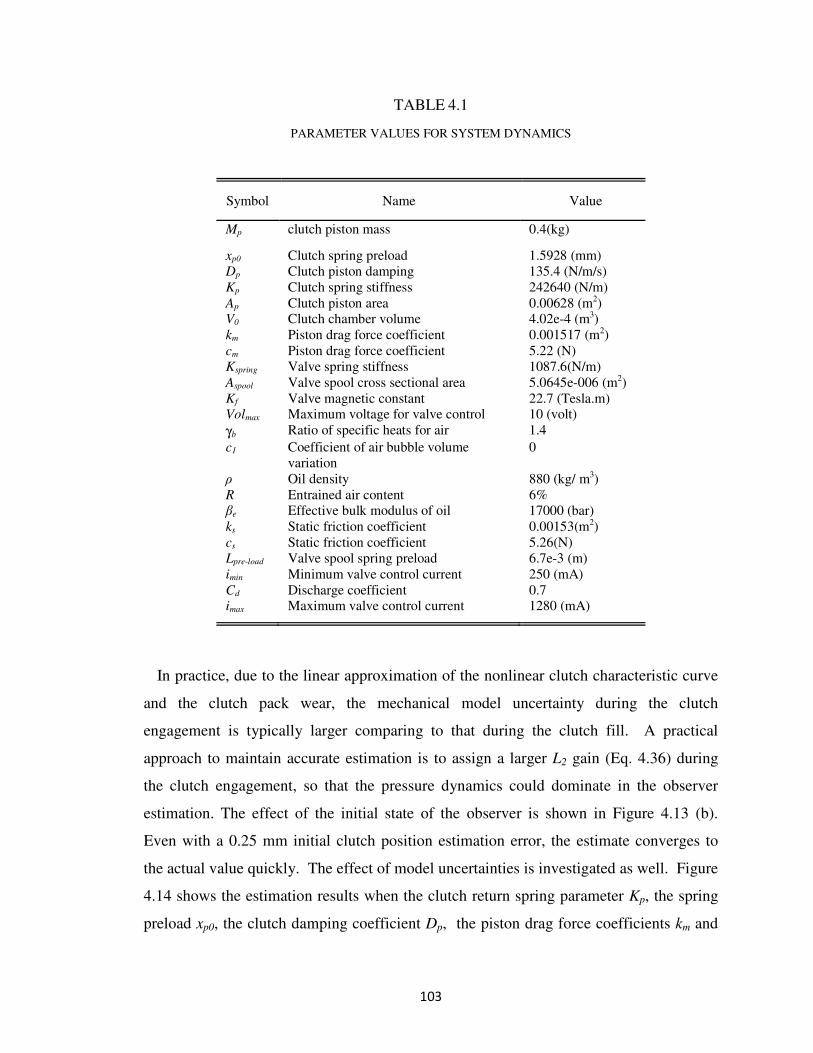
103

TABLE 4.1

PARAMETER VALUES FOR SYSTEM DYNAMICS

Symbol Name Value

Mp clutch piston mass 0.4(kg)

xp0 Clutch spring preload 1.5928 (mm)

Dp Clutch piston damping 135.4 (N/m/s)

Kp Clutch spring stiffness 242640 (N/m)

Ap Clutch piston area 0.00628 (m2)

V0 Clutch chamber volume 4.02e-4 (m3)

km Piston drag force coefficient 0.001517 (m2)

cm Piston drag force coefficient 5.22 (N)

Kspring Valve spring stiffness 1087.6(N/m)

Aspool Valve spool cross sectional area 5.0645e-006 (m2)

Kf Valve magnetic constant 22.7 (Tesla.m)

Volmax Maximum voltage for valve control 10 (volt)

γb Ratio of specific heats for air 1.4

c1 Coefficient of air bubble volume

variation

0

ρ Oil density 880 (kg/ m3)

R Entrained air content 6%

βe Effective bulk modulus of oil 17000 (bar)

ks Static friction coefficient 0.00153(m2)

cs Static friction coefficient 5.26(N)

Lpre-load Valve spool spring preload 6.7e-3 (m)

imin Minimum valve control current 250 (mA)

Cd Discharge coefficient 0.7

imax Maximum valve control current 1280 (mA)

In practice, due to the linear approximation of the nonlinear clutch characteristic curve

and the clutch pack wear, the mechanical model uncertainty during the clutch

engagement is typically larger comparing to that during the clutch fill. A practical

approach to maintain accurate estimation is to assign a larger L2 gain (Eq. 4.36) during

the clutch engagement, so that the pressure dynamics could dominate in the observer

estimation. The effect of the initial state of the observer is shown in Figure 4.13 (b).

Even with a 0.25 mm initial clutch position estimation error, the estimate converges to

the actual value quickly. The effect of model uncertainties is investigated as well. Figure

4.14 shows the estimation results when the clutch return spring parameter Kp, the spring

preload xp0, the clutch damping coefficient Dp, the piston drag force coefficients km and

104

cm, and the oil density are all perturbed by 5% . With a small L2 gain for the clutch fill

observer, the weighting on the pressure measurement is not enough to overcome the

mechanical model error, and thus the estimation discrepancy during the clutch fill phase

(from 0.1 to 0.3 second) is evident as shown in Figure 4.14 (a). The estimation can then

converge during the clutch engagement due to a larger L2 gain for the clutch engagement

observer. Figure 4.14 (b) shows the estimation result if a larger L2 gain is assigned for

the clutch fill observer. However, in practice, the value of the L2 gain is constrained.

First, as the observer design has a derivative term, large observer gain may amplify the

measurement noise. Second, increasing the gain L2 will diminish the effect of the

mechanical dynamics, which can prohibit the error convergence if the initial state error

exists.

Flow meter

Pressure

reducing

valve

In chamber

pressure

sensor

Clutch

assembly

Laser sensor

Inlet

pressure

sensor

Fig. 4.12. The experimental setup for pressure based clutch actuation. (Only pressure is used in

the real time feedback, and other sensors are installed for dynamic modeling purpose.)

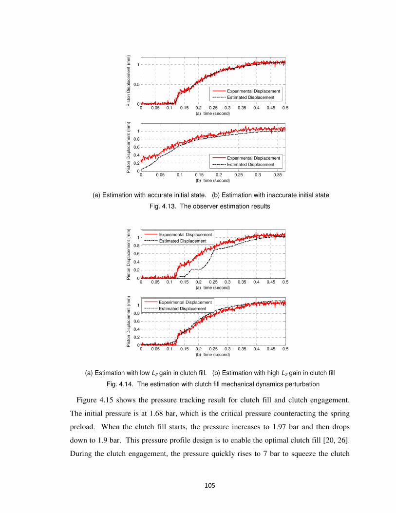
105

0 0.05 0.1 0.15 0.2 0.25 0.3 0.35 0.4 0.45 0.50

0.5

1

(a) time (second)

Pis

ton D

ispla

cem

ent

(mm

)

Experimental Displacement

Estimated Displacement

0 0.05 0.1 0.15 0.2 0.25 0.3 0.350

0.2

0.4

0.6

0.8

1

(b) time (second)

Pis

ton D

ispla

cem

ent

(mm

)



(a) Estimation with accurate initial state. (b) Estimation with inaccurate initial state

Fig. 4.13. The observer estimation results

0 0.05 0.1 0.15 0.2 0.25 0.3 0.35 0.4 0.45 0.50

0.2

0.4

0.6

0.8

1

Pis

ton D

ispla

cem

ent

(mm

)

(a) time (second)



0 0.05 0.1 0.15 0.2 0.25 0.3 0.35 0.4 0.45 0.50

0.2

0.4

0.6

0.8

1

(b) time (second)

Pis

ton D

ispla

cem

ent

(mm

)



(a) Estimation with low L2 gain in clutch fill. (b) Estimation with high L2 gain in clutch fill

Fig. 4.14. The estimation with clutch fill mechanical dynamics perturbation

Figure 4.15 shows the pressure tracking result for clutch fill and clutch engagement.

The initial pressure is at 1.68 bar, which is the critical pressure counteracting the spring

preload. When the clutch fill starts, the pressure increases to 1.97 bar and then drops

down to 1.9 bar. This pressure profile design is to enable the optimal clutch fill [20, 26].

During the clutch engagement, the pressure quickly rises to 7 bar to squeeze the clutch

106

pack. The pressure notch during engagement is to simulate the clutch slipping control.

The control signal is shown in Figure 4.16 (a) and the flow in rate is shown in Figure 4.16

(b). The first peak flow rate corresponds to the clutch fill phase and the second one

corresponds to the clutch engagement. During the clutch fill, the piston velocity is faster

comparing with that during the clutch engagement. Therefore the flow out rate induced

by the piston motion during the clutch fill is bigger, which needs more flow in rate to

increase the pressure.

29.4 29.6 29.8 30 30.2 30.4 30.6 30.8

2

3

4

5

6

7

time (second)

pre

ssure

(bar)

Real Pressure

Reference

Fig. 4.15. Pressure tracking for clutch fill and clutch engagement

One of the challenges for the clutch fill pressure control is the sudden pressure drop

once the clutch piston starts moving. Due to the rubber sealing and manufacturing

tolerance, the friction around the piston may not be balanced. This may cause the piston

to twist around the shaft, which means that the motion of the piston at different locations

is not synchronized. When the pressure increases to certain level as shown in Figure

4.10(a), one part of the piston starts moving while the other part lags behind like what is

shown in Figure 4.10(b). The twisting motion of the piston causes dynamic loading

condition change and induces abrupt flow out from the chamber. This will further result

in the sudden pressure drop. Because of the short duration of the clutch fill, the sudden

pressure drop can easily lead to an unsuccessful clutch fill pressure tracking as shown in

End of engagement

Slipping control

Clutch Fill

107

Figure 4.17. To compensate the sudden flow out and therefore maintain pressure tracking

during the dynamic loading transient, equal amount of fluid should flow in by increasing

the control valve orifice. According to the controller design (Eq.4.31), under this

scenario, there are two ways of ensuring sufficient control input. One is the accurate

piston velocity estimation 2x̂ and therefore the flow-out rate 2

ˆp

A x , which could be

translated to the required flow-in rate and thus the corresponding control input can be

determined. The other is to assign a sufficiently large sliding mode gain γ so that enough

control input will be exerted by multiplying the tracking error. In fact, it is always

desirable to compensate the pressure drop through accurate piston velocity estimation

because increasing the gain γ (Eq.4.31) can easily lead to the chattering effect. Figure

4.17(a) shows a much better tracking performance that can be attributed to the precise

nonlinear observer and a precise dynamic model.

29.4 29.6 29.8 30 30.2 30.4 30.6 30.80

5

10

(a) time (second)

contr

ol in

put

(volt)

29.4 29.6 29.8 30 30.2 30.4 30.6 30.8-1

0

1

2

3

4

(b) time (second)

flow

in r

ate

(Lpm

)

(a). Pressure control input for clutch fill and clutch engagement

(b). Flow rate for clutch fill and clutch engagement control

Fig. 4.16. Control input and the flow-in rate for clutch control

108

29.4 29.45 29.5 29.55 29.6 29.65 29.7 29.75

1.7

1.8

1.9

2

2.1

(a) time (second)

pre

ssure

(bar)

Real Pressure

Reference

1.7

1.8

1.9

2

2.1

pre

ssure

(bar)

Real Pressure

Reference

29.4 29.45 29.5 29.55 29.6 29.65 29.7 29.75

29 29.05 29.1 29.15 29.2 29.25 29.3 29.35

(b) time (second)

Fig. 4.17. Successful (a) and failed (b) pressure tracking during the clutch fill

The pressure chattering effect is shown in Figure 4.18. It is caused by a high sliding

mode gain γ (Eq.4.31). In fact, the inappropriate high gain is mostly due to the

conservative uncertainty bound of the clutch model. If the uncertainty bound is not well

modeled, a large gain is then required, which will result in rapid control signal switching

as shown in Figure 4.19(a) and Figure 4.19(b). The high frequency switching will excite

the high frequency unmodeled dynamics and thus cause the chattering effect. Figure

4.19(b) shows the flow-in rate, which also exhibits the high frequency flow-in rate

switching. The chattering effect is more severe in the high pressure range, where the

hydraulic system is stiffer and thus more sensitive to the control command switching.

Therefore, an appropriate sliding mode control gain should be selected based on the

model uncertainty.

109

31.2 31.4 31.6 31.8 32 32.2 32.4 32.6

2

3

4

5

6

7

time (second)

pre

ssure

(bar)

Real Pressure

Reference

Fig. 4.18. Pressure chattering effect due to large uncertainty bound

31.2 31.4 31.6 31.8 32 32.2 32.4 32.60

5

10

(a) time (second)

contr

ol in

put

(volt)

31.2 31.4 31.6 31.8 32 32.2 32.4 32.6-1

0

1

2

3

4

(b) time (second)

flow

in r

ate

(Lpm

)

(a). Pressure control input for clutch fill and clutch engagement

(b). Flow rate for clutch fill and clutch engagement control

Fig. 4.19. Control input and flow rate data.

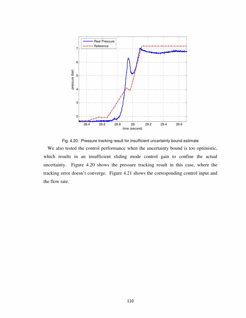
110

28.4 28.6 28.8 29 29.2 29.4 29.6

2

3

4

5

6

7

time (second)

pre

ssure

(bar)

Real Pressure

Reference

Fig. 4.20. Pressure tracking result for insufficient uncertainty bound estimate

We also tested the control performance when the uncertainty bound is too optimistic,

which results in an insufficient sliding mode control gain to confine the actual

uncertainty. Figure 4.20 shows the pressure tracking result in this case, where the

tracking error doesn’t converge. Figure 4.21 shows the corresponding control input and

the flow rate.

111

28.4 28.6 28.8 29 29.2 29.4 29.60

5

10

(a) time (second)

contr

ol in

put

(volt)

28.4 28.6 28.8 29 29.2 29.4 29.6-1

0

1

2

3

4

(b) time (second)

flow

in r

ate

(Lpm

)

Fig. 4.21. Control signal and the flow rate for insufficient uncertainty bound estimate

4.6 Conclusion

This chapter presents a systematic approach for the pressure based clutch fill and

engagement control of wet clutches in automatic, dual clutch, or hybrid transmissions.

The clutch fill and engagement controls are critical for the clutch-to-clutch shift

technology, which is the key enabler for fuel efficient, compact and low cost transmission

designs. The main challenges of the pressure based clutch control design lie in the

complex dynamics, the on/off behavior during the clutch fill phase, the pressure

chattering effect induced by inappropriate control gain design, and the precise pressure

tracking requirement during the dynamic loading condition transient. To address these

challenges, first, a dynamic model capturing the bulk modulus variation and the piston

motion wiggling effect is constructed based on extensive experimental results. A precise

estimation of the bounds for unmodeled dynamics is also obtained. Then a sliding mode

based robust controller is designed to track the desired pressure. To avoid chattering, the

controller gain is designed based on the non-conservative uncertainty bound. To ensure

precise tracking, an observer is designed to estimate the clutch piston motion, which is a

necessary term in the controller structure to further alleviate the high gain demand. In

addition, the observer estimation can also be used to diagnose the clutch fill status.

112

Finally, experimental results show the effectiveness of the proposed control methods.

Future works include the investigation with a miniature pressure sensor, the model

uncertainty calibration in various environments, and the vehicle test of the proposed

control algorithm.

113







[3] Sun, Z. and Hebbale, K.V., “Challenges and opportunities in automotive transmission


June 8-10, 2005.




[5] Bai, S., Moses, R.L, Schanz, T. and Gorman, M.J. “Development of A New Clutch-

to-Clutch Shift Control Technology”. SAE Technical Paper 2002-01-1252.


Transmission Control Strategy”. SAE Technical Paper 2007-01-1313.


Automatic Transmission.” Proc. Instn Mech. Engrs Part D: Journal of Automobile

Engineering. Volume 217, Number 4/2003, pp 289-298.

[8] Zhang, Y., Chen, X., Zhang, X., Jiang, H., and Tobler, W., “Dynamic Modeling and



[9] T. Grewe, B. Conlon, and A. Holmes. Defining the General Motors 2-Mode Hybrid



electric vehicle during mode change. SAE Technical Paper Series 2009-01-0228,

2009.

[11] M. Levin, et. al. Hybrid powertrain with an engine-disconnection clutch. SAE


114

[12] Glielmo, L., Iannelli, L., Vacca, V., “Gearshift Control for Automated Manual

Transmissions”, IEEE/ASME Transactions on Mechatronics, Vol. 11, No.1, pp. 17-

26, Feb., 2006.

[13] Langjord, H., Johansen, T., “Dual-Mode Switched Control of an

Electropneumatic Clutch Actuator,” IEEE/ASME Transactions on Mechatronics, in

press, 2010.

[14] Montanari, M., Ronchi, F., Rossi, C., Tilli, A., Tonielli, A., “Control and


Journal of Control Engineering Practice, Vol. 12, Issue 11, pp. 1369-1379, Nov,

2004.

[15] Horn, J., Bamberger, J., Michau, P., Pindl, S., “Flatness-based Clutch Control for

Automated Manual Transmissions”, Journal of Control Engineering Practice, Vol. 11,

Issue 12, pp. 1353-1359, Dec., 2003.

[16] Sanada, K., Kitagawa, A., “A Study of Two-degree-of-freedom Control of

Rotating Speed in an Automatic Transmission, Considering Modeling Errors of a

Hydraulic System”, Journal of Control Engineering Practice, Vol. 6, Issue 9, pp.

1125-1132, Dec., 1998.

[17] Gao, B., Chen, H., Sanada, K., Hu, Y., “Design of Clutch-Slip Controller for

Automatic Transmission Using Backstepping,” IEEE/ASME Transactions on

Mechatronics, in press, 2010.

[18] Gao, B., Chen, H., Sanada, “A Reduced Order Nonlinear Clutch Pressure

Observer for Automatic Transmission,” IEEE Transactions on Control Systems

Technology, Vol. 18, Issue.2, pp. 446-453, March., 2010.

[19] Yu, J., Chen, Z., and Lu, Y., “ The Variation of Oil Effective Bulk Modulus With

Pressure in Hydraulic Systems”, Journal of Dynamic Systems, Measurement, and

Control, Vol. 116, No. 1, pp. 146-150, March, 1994.

[20] Song, X., Mohd Zulkefli, A., and Sun, Z., “Automotive Transmission Clutch Fill

Optimal Control: An Experimental Investigation”, Proceedings of 2010 American

Control Conference, Baltimore, MD, USA, June 30-July 2nd, 2010.

115

[21] Song, X., Sun, Z., Yang, X., Zhu, G., “Modeling, Control and Hardware-in-the-

Loop Simulation of an Automated Manual Transmission”, Proc. Inst Mech. Engrs,

Part D, Journal of Automobile Engineering, Vol. 224, pp.143-159, 2010.

[22] Song, X., Zulkefli, A., Sun, Z. and Miao, H., “Modeling, Analysis, and Optimal



March, 2010.

[23] Karnopp, D., “Computer Simulation of Stick-Slip Friction in Mechanical

Dynamic Systems”, Journal of Dynamic Systems, Measurement, and Control, Vol.

107, No. 1, pp. 100-103, March, 1985.

[24] Khalil, H., Nonlinear Systems, Third Edition, Pearson Education, Inc., 2002.

[25] Crassidis, J.L. and Junkins, J.L. “Optimal Estimation of Dynamic Systems”.


Express LLC, 2004.

[26] Miao, H., Sun, Z., Fair, J., Lehrmann, J., Harbin, S. “Modeling and Analysis of

the Hydraulic System for Oil Budget in an Automotive Transmission”. Proceedings

of ASME 2008 Dynamic Systems and Control Conference, Ann Arbor, Michigan,

USA, Oct., 2008.

[27] Vasca, F., Iannelli, L., Senatore, A., Reale, G. , "Torque Transmissibility

Assessment for Automotive Dry-Clutch Engagement," IEEE/ASME Transactions on

Mechatronics, , no.99, pp.1-10, in press.

116

Chapter 5

The Clutch Level Design-- Design, Modeling and Control of a

Novel Automotive Transmission Clutch Actuation System

The pressure based clutch control method introduced in Chapter 4 is expected to be

robust and effective. However, the requirement for pressure sensor feedback inevitably

increases cost and assembly complexity. For mass production, it is desirable to have a

low cost and robust feedback mechanism without any sensor installed. Inspired by these

requirements, an alternate clutch feedback control approach without sensor measurement

is proposed in this chapter.

5.1 Introduction

The increasing demand of more fuel efficient automotive propulsion systems

requires further improvement of the power transmission technologies. In recent years,

many different types of transmissions, such as the six or more speeds automatic

transmission, the dual clutch transmission, the automated manual transmission, and the

electrically variable transmission have been developed by automotive manufacturers.

Although different in design, they share common challenges on the smooth and efficient

gear shift. The key issue to address is the precise and efficient operation of the clutch

actuation system [1-2].

One example where a precise clutch actuation is critical is the clutch to clutch shift

technology [3-6], which is the key enabler for a compact, low cost and efficient automatic

transmission. The basic concept is to control the engagement and disengagement of the

on-coming and off-going clutch packs to realize the gear shift [4]. To have a smooth

shift, it is crucial to place the on-coming clutch piston at a pre-determined position before

the shift, and this again highly depends on a precise and robust clutch control.

Due to the high power density of electro-hydraulic systems, the most common

configuration is to use wet clutches with hydraulic actuated pistons in automatic and

hybrid transmissions [7]. A schematic diagram of the hydraulic clutch actuation system

is shown in Figure 5.1. Suppose initially the clutch is disengaged, then the piston is

117

separate from the clutch pack. Right before the clutch engagement, pressurized fluid will

flow into the clutch chamber and push the clutch piston towards the clutch pack. This

process is called clutch fill. At the end of clutch fill, high pressure fluid will continue

flowing in and then push the piston to squeeze the clutch pack for clutch engagement to

transfer power. It is crucial to have the piston arrive at the predetermined position at the

end of clutch fill, otherwise the power transfer during the following engagement phase

will be disturbed and therefore cause serious driveline vibration problem [2].

Supply

Fluid

Orifice

Piston

Piston Seal

Return Spring

Clutch Pack

Clutch

Chamber

Supply

Fluid

Orifice

Piston

Piston Seal

Return Spring

Clutch Pack

Clutch

Chamber

Supply

Fluid

Orifice

Piston

Piston Seal

Return Spring

Clutch Pack

Clutch

Chamber

Figure 5.1 Schematic diagram of transmission clutch system

There are three main challenges associated with a precise clutch fill. First, the

system is very sensitive. Even a small perturbation of the clutch fill displacement and fill

time could easily cause an over-fill or an under-fill [2], which will degrade the shift

quality. Second, the clutch piston typically travels 1~2 mm within 0.2 second during the

clutch fill, which requires an accurate and swift actuation. Third, for mass production

purpose, the clutch control system must be low cost, physically compact and robust.

However, the traditional approach is in an open loop fashion due to the lack of a feedback

sensor, which requires extensive calibration and also complicated upstream hydraulic

control system. To address this problem, forming a feedback control loop is necessary.

Ref [7] analyzes the unique nonlinear clutch actuation dynamics and proposes a sliding

mode pressure based control method, which requires a pressure sensor in the clutch

chamber. Different from Ref [7], in this chapter, an alternate clutch feedback control

approach will be introduced, which relies on a new electro-hydraulic mechanism

adopting the internal feedback concept [8] and enables a robust and precise control

118

without any sensor installed.

The new mechanism relays the clutch piston motion to the control spool position via

a built-in hydra-mechanical feedback channel to achieve precise and robust piston motion

without any feedback sensor. This design not only reduces the cost of forming an

electronic controller, but also avoids the external nonlinear feedback controller synthesis

considering the complex hydraulic clutch dynamics [7].

The rest of the chapter is organized as follows. Section 5.2 presents the system design

and working principle of the new mechanism. Section 5.3 presents mechanical design of

the new system and its dynamic modeling. To this end, simulation and experimental

results are presented in section 5.4 to show the preciseness and robustness of the

proposed system.

5.2 System Design and working principle

In this section, the proposed internal feedback clutch actuation system working

principle will be presented first, and then its advantage over the conventional clutch

actuation will be explained.

5.2.1 System design and working principle

Figure 5.2a shows the simplified schematic diagram of the proposed clutch actuation

system, which mainly consists of two on/off valves, an internal feedback spool ( IFS), a

IFS return spring, a feedback channel and the clutch assembly. The internal feedback

spool (IFS) controls the opening orifice between the supply pressure and the clutch

chamber, and is the key component of the whole mechanism.

The following are the operating sequences of the system.

(1) When the clutch piston is at the initial disengaged position (Figure 5.2a), the on/off

valve 1 connects the IFS orifice, AIFS, to the fluid tank. The pressure inside the clutch

chamber is low, so the clutch piston will be kept at the disengaged position by the return

spring.

(2) When the clutch fill process begins, the on/off valve 1 is energized to connect the IFS

orifice to the supply pressure. Pressurized fluid then enters the clutch chamber through

the IFS orifice, counteracting the spring force and pushes the clutch piston to the right.

119

On the other side, the on/off valve 2 at the feedback exhaust port is closed to block the

fluid inside the piston feedback chamber from flowing out to the tank. Therefore the

clutch piston motion will squeeze the fluid in the piston feedback chamber to the IFS

chamber through the feedback channel, which then drives the IFS upward (Figure 5.2b).

As the IFS moves upward, the IFS orifice area gradually decreases. This restricts the flow

through the IFS orifice which then slows down the pressure rise in the clutch chamber.

The clutch piston and the IFS continue to move in a synchronized fashion until the

IFS orifice is cut off, which then separates the clutch chamber from the supply pressure.

At the end of the clutch fill, the piston arrives at the final position just before engaging

the clutch packs, and the IFS stops and the IFS orifice area is completely closed.

From the analysis above, it can be observed that the clutch piston displacement is fed

back through the IFS orifice area, which regulates the fluid pressure inside the clutch

chamber. This internal feedback structure ensures robust and precise motion of the clutch

fill process. The feedback structure also guarantees a smoothly decreasing clutch piston

velocity profile as it approaches the clutch fill final position.

(3) After the clutch fill, the clutch packs are ready to be engaged for torque transmission.

When the clutch engagement starts, the clutch piston needs to be pushed further to

squeeze the clutch. This can be realized by opening the on/off valve 2 at the exhaust port

to release the fluid in the feedback chamber to the tank. As a result, the pressures in the

piston feedback chamber and the IFS chamber will drop, and subsequently the IFS return

spring can push the IFS downwards until the IFS orifice is fully open. The supply

pressure, Ps, which now gets reconnected to the clutch chamber, will push the clutch

piston further to squeeze the clutch packs.

(4) During the clutch disengagement, the clutch piston needs to move back to its

initial position so that the clutch packs will be released. For that, the on/off valve 1 is de-

energized to connect the IFS orifice to the low pressure tank. The return spring will then

push the piston back to the disengaged position.

120

Solenoid on/off

valve 1

Solenoid on/off

valve 2

Supply Pressure

Tank

Figure 5.2a. Schematic diagram of the proposed clutch actuation control system

Tank

Figure 5.2b. Piston and IFS motion during clutch fill

Figure 5.2. IFS system design and working principle

5.5.2 Advantages of the new mechanism

The control block diagram of the IFS clutch actuation system is shown in Figure 5.3,

which shows that the proposed mechanism consisting of the IFS, the clutch piston, and

the on/off valve can be represented in a feedback loop.

121

Control Element

(Spool orifice)

Plant

(Clutch)

Piston

Displacement

Feedback Element

( Displacement ratio)

Spool

Displacement

Spool Opening

Area

Figure 5.3. Feedback control diagram

There are two key merits of this new mechanism regarding the clutch control. First,

instead of designing a nonlinear controller considering the complex nonlinear hydraulic

dynamics, the proposed IFS clutch actuation system can realize a fast, precise and robust

nonlinear control only by self-regulating the IFS spool orifice with the hydra-mechanical

feedback rather than sensor measurement. The orifice area control automatically

regulates the clutch chamber pressure and thus enables a smooth and precise clutch piston

velocity and displacement profile. Second, ensuring a precise and robust clutch fill with

the IFS system at the clutch level will enable the simplification of the upstream hydraulic

control system including the control valves, the electronic control devices and their

accessories [9]. This will not only improve the transmission system compactness, but can

also alleviate the external control calibration efforts.

5.3 Mechanical Design and System Modeling

In this section, we will describe the IFS system mechanical design, targeting

convenient assembly with the in production six speed automatic transmissions. Then

based on the mechanical design, the dynamics model for the clutch fill process will be

presented.

5.3.1 Mechanical System Design

The IFS mechanical system assembly shown in Figure 5.4 consists of the IFS body

with chambers built inside, an IFS spool, a spring, two on/off valves and a clutch

actuator. During the clutch fill, the pressure supply fluid will flow into the input chamber,

passing the intermediate actuation chamber and the clutch orifice and finally reach the

122

clutch chamber (the path shown in solid red line in Figure 5.4). Note that the clutch

orifice is a ring shaped long channel surrounding but not connecting to the feedback

channel, and it’s also connecting the intermediate actuation chamber and the clutch

chamber. Once the high pressure fluid pushes the clutch piston forward, the piston will

squeeze the fluid in the piston feedback chamber into the feedback channel and finally to

the IFS chamber (the path shown in blue dashed line in Figure 5.4). Then the IFS piston

will move to the left, counteracting the IFS spring and gradually closing the IFS orifice.

One of the most important design parameters is the IFS orifice, which is fabricated

into a rectangular shaped slot. It acts as a crucial control variable that regulates the clutch

chamber pressure by controlling the size of the IFS orifice area AIFS with respect to the

IFS spool displacement XIFS during the clutch fill process. It determines the final clutch

fill displacement, as the clutch piston will stop once the IFS orifice is cut off by the IFS

spool. Therefore the orifice length should be designed according to the desired clutch fill

final piston displacement.

5.3.2 IFS Modeling

The dynamics model of the IFS clutch control system includes the mechanical models

of the clutch piston and the IFS spool, the pressure dynamics of the input pressure

chamber, the intermediate actuation chamber, the clutch chamber, and the IFS chamber

respectively. The piston feedback chamber is regarded as the same chamber as the IFS

chamber because the feedback channel connecting these two are big enough to allow

throttleless assumption.

The clutch and the IFS mechanical dynamics are described as

( )( ) ( )

( , )

pis pis c cen c IFS cb c pis preload pis

pis pis drag c pis

M X P P A P A K X X

D X F P X

= + − − +

− −

��

� � (5.1)

( )

_

( ) ( )

( )

IFS IFS IFS cen IFS IFS IFS preload IFS

IFS IFS drag IFS IFS

M X P P A K X X

D X F X

= + − +

− −

��

� � (5.2)

123

where Mpis is the clutch piston mass, Xpis is the clutch piston displacement, Pc is the

clutch chamber pressure, Pcen is the average fluid centrifugal pressure as discussed in

[10], Ac is the clutch piston area, Acb is the clutch piston feedback area (the piston surface

facing the piston feedback chamber), Kc is the clutch piston spring constant, Xpreload(pis) is

the preload of the clutch piston spring, Dpis is the clutch damping coefficient. Fdrag is the

piston seal drag force, which is dependent on the piston motion. It is modeled as:

( ) ( ) ( 0)

( 0)

m c cen m pis pis

drag

stick pis

k P P c sign X XF

F X

+ + × ≠ = =

� �

� (5.3)

where km and cm are constant, and Fstick is the static stick friction force from the

Kanopp’s stick-slip model [11]. Further detailed formulation of the mechanical dynamic

model can be found in our recent work [12].

MIFS is the IFS mass, XIFS is the IFS displacement, PIFS is the IFS/piston feedback

chamber pressure, AIFS is the IFS spool cross sectional area, KIFS is the IFS spring

constant, Xpreload(IFS) is the preload of the IFS spring and DIFS is the IFS damping

coefficient. In addition, the spool drag force Fdrag_IFS is defined as:

( )_

_

_

( 0)

( 0)

m s IFS IFS

drag IFS

stick IFS IFS

c sign X XF

F X

× ≠=

=

� �

� (5.4)

where cm_s is the spool friction constant, and Fstick_IFS is the static stick friction force

of the IFS spool.

124

Supply

fluid

IFS spring

IFS spool

Intermediate

actuation

chamber

Input

chamber

Solenoid

on/off valve 1

IFS chamber

Clutch spring

Piston dam

Piston feedback

chamber

Feedback channel

Clutch orifice

Clutch chamber

Clutch piston

Clutch assembly

Solenoid

on/off valve 2

Supply

fluid

IFS spring

IFS spool

Intermediate

actuation

chamber

Input

chamber

Solenoid

on/off valve 1

IFS chamber

Clutch spring

Piston dam

Piston feedback

chamber

Feedback channel

Clutch orifice

Clutch chamber

Clutch piston

Clutch assembly

Solenoid

on/off valve 2

Fig 5.4. IFS system mechanical design drawing

The volumetric flow rates through the input chamber orifice, the intermediate

actuation chamber orifice, and the clutch orifice can be described as

2sgn( )

s in

in in d s in

P PQ A C P P

ρ

−= ⋅ − (5.5)

2sgn( )

in m

IFS IFS d in m

P PQ A C P P

ρ

−= ⋅ − (5.6)

125

2sgn( )

m c

c c d m c

P PQ A C P P

ρ

−= ⋅ − (5.7)

where Cd is the discharge coefficient, ρ is the transmission fluid density, Ps is the supply

pressure, Pin is the input chamber pressure, Pm is the intermediate actuation chamber

(Figure 5.4) pressure and Pc is the clutch chamber pressure. Ain is the orifice area

between the supply channel and the input chamber, AIFS is the IFS orifice opening area

between the input chamber and the intermediate chamber, Ac is the ring shaped orifice

between the intermediate chamber and the clutch chamber as shown in Figure 5.4. In

particular, the IFS orifice area AIFS keeps changing during clutch fill and is determined by

the IFS spool displacement. It can be described as:

( )IFS IFS

A w d X= × − (5.8)

where w is the slot width of the rectangular shaped IFS orifice, and d is the length of the

slot orifice.

The pressure dynamics in the input chamber, the intermediate chamber, the clutch

chamber and IFS chamber can be described as:

( )( )in

in in IFS

in

PP Q Q

V

β= −� (5.9)

( )( )m

m IFS c

m

PP Q Q

V

β= −� (5.10)

( )( )c

c c c pis

c

PP Q A X

V

β= −� � (5.11)

( )( )IFS

IFS cb pis IFS IFS

IFS

PP A X A X

V

β= −� � � (5.12)

where Vin is the input chamber volume, Vm is the chamber volume of the intermediate

actuation chamber, and Vc is the clutch chamber volume given by

0c c pis pisV V A X= + (5.13)

126

where Vc0 is the initial volume of the clutch chamber. In addition, VIFS is the IFS chamber

volume, which depends on the clutch piston and the IFS spool displacement and is given

by:

0IFS IFS IFS IFS pis pisV V A X A X= + − (5.14)

where VIFS0 is the initial value of the lumped IFS chamber, feedback channel and the

piston feedback chamber volume before the clutch fill. In addition, the bulk modulus β is

modeled as a function of the chamber pressure because the air entrained in the low

pressure oil could cause the bulk modulus variation. The variation is modeled with

respect the chamber pressure Pr (Pr may refer to any chamber pressure) as [13]:

1 1/5

1 1/5 5 5

1

(1 10 )( )

(1 10 ) 10 (1 )( / 10 )

b

b

e r

r

r r e b r

PP

P R c P P

γ

γ

ββ

β γ

+−

+− −

+=

+ + − − − (5.15)

where βe is the bulk modulus in ideal fluid with no air entrained, γb is the ratio of specific

heats for air, c1 is the coefficient of air bubble volume variation due to the variation of the

ratio of the entrained air and dissolved air content in oil, R is the entrained air content by

volume in oil at atmosphere pressure. βe, R, γb and c1 are fixed when the oil temperature

and pumping conditions are constant.

5.4. Simulation and Experimental Results

The designed internal feedback mechanism is fabricated for experimental

verification. The internal channels are directly built inside the IFS body. The IFS clutch

control test bed is shown in Figure 5.5. The main parts include a servo motor, an

automotive transmission pump, a pilot-operated proportional relief valve, two on/off

valves, a flow meter, two pressure sensors, a clutch mounting device/fixture, a

displacement sensor, a power supply unit with servo amplifier and an XPC-target real

time control system. In particular, one on/off valve controls the supply oil input into the

clutch chamber, and the other controls the hydraulic oil injection into the internal

feedback chamber for back pressure. In addition, as a note here, the sensors in the test

bed are not used for the clutch control, but only for performance verification purpose.

The IFS system operation requires no measurement feedback.

127

Relief valve for

high pressure supply

Fluid channel for

internal feedback chamber oil injection

Displacement

sensor

Pressure

sensors

IFS bodyClutch

Air

bleeding

port

On/off

valve 1

On/off

valve 2

Figure 5.5. IFS clutch actuation test bed

The clutch fill experimental results are shown in Figure 5.6-Figure 5.9. The supply

pressure is kept at 13 bar using a pressure relief valve. First, after injecting hydraulic oil

into the internal feedback channel for back pressure, the internal feedback IFS chamber is

cut off by the on/off valve 2. Then the on/off valve 1 connecting the supply pressure with

the input chamber is switched to open, thus high pressure fluid can flow into the clutch

chamber and then push the clutch piston to move. Over 30 groups of clutch fill tests are

conducted and all of them show good repeatability. The clutch piston displacements from

six representative tests are shown in Figure 5.6, which clearly shows that the

displacement trajectories from different tests can almost overlap each other.

128

0 0.05 0.1 0.15 0.2 0.25

0

0.2

0.4

0.6

0.8

1

time (s)

Clu

tch P

isto

n

dis

pla

cem

ent

(mm

)

test1

test2

test3

test4

test5

test6Modeling Error

Figure 5.6. Multiple tests for clutch piston displacement and the dynamics modeling

error of the clutch piston motion

0 0.05 0.1 0.15 0.2 0.251

2

3

4x 10

5

time (s)

Inte

rmedia

te

cham

ber

pre

ssure

(P

a)

Experiment

Simulated

Figure 5.7. Intermediate actuation chamber pressure

0 0.05 0.1 0.15 0.2 0.251.2

1.3

1.4

1.5

1.6

1.7x 10

5

time (s)

IFS

cham

ber

pre

ssure

(pa)

Experiment

Simulated

Figure 5.8. IFS chamber pressure

129

0 0.05 0.1 0.15 0.2 0.250

0.005

0.01

time (s)

IFS

spool dis

pla

cem

ent

(m)

Experiment

Simulated

Figure 5.9. IFS spool displacement

At the start of the clutch fill process, the intermediate actuation chamber pressure

quickly goes up due to the in-coming high pressure fluid as shown in Figure 5.7. At 0.05

seconds, the pressure in the intermediate actuation chamber (Figure 5.7) along with the

clutch chamber is high enough to overcome the return spring force to push the clutch

piston to move, then subsequently the clutch chamber pressure suddenly drops due to the

piston motion induced out-flow. The pressure inside the clutch chamber is then kept in an

appropriate level to keep moving the clutch piston forward. The pressure in the piston

feedback and IFS chamber will then go up (Figure 5.8) due to the squeezing by the clutch

piston, and thus push the IFS spool to close the IFS orifice. Once the IFS spool travels to

the end and therefore cut off the IFS orifice as shown in Figure 5.9, the clutch piston

stops at around 0.175 seconds. At the end of clutch fill, the clutch piston travels 1 mili-

meter robustly as shown in Figure 5.6, which is exactly the desired clutch fill final

displacement.

Finally, the system parameters are measured and identified as shown in Table I. The

IFS system dynamics model built in Section III is then verified by simulation. The clutch

piston motion dynamics modeling error is shown in Figure 5.6, and the dynamics

modeling matching results for the intermediate actuation chamber pressure, the IFS

chamber pressure and the IFS spool displacement are shown in Figures 5.7-5.9

respectively. It’s assumed that the input on/off valve 1 in Figure 5.5 is opened 25% of the

fully open orifice area in 250 mili-second. As can be seen, the dynamics model matches

well with the experimental data and thus could be used for further design modification

and analysis.

130

TABLE 5.1. SYSTEM PARAMETERS

Symbol Name Value

Mpis clutch piston mass 0.4(kg)

Xpreload(pis) Clutch spring preload 4.15 (mm)

Dpis Clutch piston damping 46926 (N/m/s)

Kc Clutch spring stiffness 108899 (N/m)

Ac Clutch piston front area 0.010681 (m2)

Acb Clutch piston back area 0.010681 (m2)

MIFS IFS spool mass 0.256 (kg)

KIFS IFS spring stiffness 1517.9(N/m)

AIFS IFS spool cross sectional area 0.000992 (m2)

Xpreload(IFS) IFS spring preload 10.063 (mm)

DIFS IFS spool damping 438.96 (N/m/s)

km Piston drag force coefficient 0.0016229 (m2)

cm Piston drag force coefficient 50.927 (N)

ks Piston stick friction coefficient 0.0046229 (m2)

cs Piston stick friction coefficient 122.927 (N)

cm_s IFS spool drag force coefficient 24.521 (N)

cstick_s IFS spool stick friction coefficient 26 (N)

w Slot width of IFS orifice 1.988 (mm)

d Length of the IFS slot orifice 7.3 (mm)

Vin Input chamber volume 1.2455e-4 (m3)

Vm Intermediate chamber volume 1.8095e-5 (m3)

Vc0 Clutch chamber initial volume 1.8277e-6 (m3)

VIFS0 IFS chamber initial volume 6.8e-4 (m3)

Ain Input chamber orifice area 2.4675e-5 (m2)

Aco Clutch chamber orifice area 1.5025e-5 (m2)

γb Ratio of specific heats for air 1.4

c1 Coefficient of air bubble volume

variation

-9.3e-6

ρ Oil density 880 (kg/ m3)

R Entrained air content 7.5%

βe Effective bulk modulus of oil 17000 (bar)

Cd Discharge coefficient 0.7

5.5. Conclusion

This chapter presents a novel transmission clutch actuation system with internal

feedback. The internal feedback mechanism relays the clutch piston motion to the control

spool position via a built-in feedback channel to achieve robust and precise clutch fill

without any sensor measurement. The clutch fill process, which is traditionally

131

controlled in an open loop fashion due to the absence of a sensor, could therefore be

controlled precisely using the internal feedback mechanism. The internal feedback

system is designed for convenient assembly with the in-production automatic

transmission by adding a few components, and is fabricated and tested in the clutch

control test bed. Multiple tests demonstrate the accuracy and reliability of the clutch fill

using the developed system, and the experimental and modeling results are presented.

Future work includes more compact IFS system design and fabrication, the IFS orifice

optimization for the optimal clutch fill, and finally the in-vehicle tests.

132




[2] Sun, Z. and Kumar, H., “Challenges and opportunities in automotive transmission


June 8-10, 2005.









Automatic Transmission.” Proc. Instn Mech. Engrs vol. 217 Part D: J. Automobile


[7] Song, X. and Sun, Z., “Pressure Based Clutch Control for Automotive Transmissions

Using a Sliding Mode Controller”, in press, IEEE Transactions on Mechatronics,

2011.

[8] Sun, Z., “Electro-Hydraulic Fully Flexible Valve Actuation System with Internal

Feedback”, ASME Transactions on Journal of Dynamic Systems, Measurement and

Control, Vol. 131, 024502, March 2009.

[9] Miao, H., Sun, Z., Fair, J., Lehrmann, J., Harbin, S. “Modeling and Analysis of the


ASME 2008 Dynamic Systems and Control Conference, Ann Arbor, Michigan, USA,

October 20-22, 2008

[10] Song, X., Sun, Z., Yang, X., Zhu, G., “Modeling, Control and Hardware-in-the-Loop

Simulation of an Automated Manual Transmission”, Proc. Inst Mech. Engrs, Part D,

Journal of Automobile Engineering, Vol. 224, pp.143-159, 2010.

133

[11] Karnopp, D., “Computer Simulation of Stick-Slip Friction in Mechanical Dynamic

Systems”, Journal of Dynamic Systems, Measurement, and Control, Vol. 107, No. 1,

pp. 100-103, March, 1985.

[12] Song, X., Mohd Zulkefli, A., Sun, Z. and Miao, H., “Automotive Transmission

Clutch Fill Control Using a Customized Dynamic Programming Method”, in press,

ASME Transactions on Journal of Dynamic Systems, Measurement and Control,

2010.

[13] Yu, J., Chen, Z., and Lu, Y., “ The Variation of Oil Effective Bulk Modulus With



134

Chapter 6

The Driveline Level Design--Automated Manual Transmission

(AMT) Optimal Clutch Engagement

Chapters 2 to Chapter 5 focus on the clutch level control. The control of the clutch

actuation alone will not guarantee satisfactory performance of the whole power

transmission system. Efficient and successful coordination with the driveline is another

important factor. Failure in coordination will result in a less efficient or even perturbed

power transmission. Therefore, in this chapter, the power transmission problem will be

studied in the driveline level, by considering the clutch control and its coordination with

driveline together. This study will be based on the automated manual transmission

(AMT) optimal clutch engagement problem.

6.1. Introduction

The automated manual transmission (Figure 6.1) is a new type automatic

transmission combining the benefits of both automatic and manual transmissions. A

vehicle equipped with the automated manual transmission (AMT) should be operated in

the same way as the automatic transmission, but the fuel economy should be highly

improved comparing with the AT system. However, poorly designed AMT system will

cause undesired vehicle vibration during gear shifts due to the torque interruption. This

undesirable characteristic of the AMT system is actually the bottle neck for its wide

application and competition with the automatic transmission system in the market. But

this technical difficulty also brings in a great research opportunity, given the volatile fuel

price and environmental concerns.

135

Figure 6.1. The AMT schematic diagram

The automated manual transmission [10-12] shares similar mechanical structure

with the manual transmission system. Different from the manual transmission, the clutch

and gearshift are controlled automatically by the AMT microcontroller. The most critical

operation is the clutch launching and gearshift slipping control, which must satisfy

several performance requirements: short gearshift duration and smooth gearshift with

improved vehicle fuel efficiency.

To achieve those performance objectives, it is very important to build an effective

dynamic model to study the dynamic characteristics of the AMT system. Moreover, it is

also desirable to manage the control and motion strategy of the clutch engagement, which

is the key factor for drivability and fuel consumption of the AMT system. The desired

control method should result in smooth clutch engagement without lurch, and minimize

energy loss due to the clutch slip for good fuel economy. In fact, in order to achieve

these objectives, researches related to the clutch engagement during the gearshift phase

have been widely explored. In [10], the control method to track reference clutch torque is

presented to achieve the desirable performance. In [12], an approach for computing the

desirable engine speed during gearshift is proposed. In [13], a neuro-fuzzy approach is

implemented. In [14], a model based backstepping methodology is used to design the

gearshift control in the AMT system.

However, in spite of the extensive literature on AMT control, the control

methodology of the AMT system is still not mature for its wide applications. The main

challenge lies in the clutch torque interruption during engagement and the coordination of

136

the engine and the transmission. To improve the control design and validation process, a

practical model and rapid prototyping system is necessary. In this chapter, a Simulink

AMT model is developed for AMT control strategy development and validation.

In addition, few papers have been published that offer a systematic approach to

obtain the desired trajectory of the clutch torque input, which is the key for the minimal

energy loss control. Reference [10] presents a method to control the clutch torque based

upon the engine and the clutch reference velocities, but it doesn’t provide the optimal

clutch torque for smooth gearshift without vibration. Reference [15] provides a control

strategy based on Linear Quadratic control, but the quadratic cost function used is not the

actual energy loss cost function. In this chapter we will explore the possibility of using

Dynamic Programming method to design the optimal clutch and engine velocity/torque

trajectory during clutch engagement. Although the Dynamic Programming method

requires tremendous computational throughput, it is capable of providing optimal

solution based upon non-quadratic cost function and the given nonlinear dynamic model.

Finally the optimal control generated from DP will be compared with regular non-optimal

PID control.

This chapter is organized as follows. In Section 6.2, models of the driveline and the

dry clutch are discussed. In Section 6.3, four different operating phases of the AMT are

analyzed. The controllers corresponding to each phase are also presented. In addition, the

possibility of using the Dynamic Programming method to generate the optimal clutch

torque control input is investigated. Simulation results of the AMT system performance

and the optimized clutch torque trajectory are presented in Section 6.4.

6.2. System Modeling

In this section, the dynamics of the driveline system and major subsystems of the

AMT system are modeled. The clutch actuator model is well studied in Chapter 3 and

thus will not be presented in detail here.

6.2.1 Driveline Modeling

The driveline dynamic modeling has been well studied in the literature [16-21].

Reference [2] presented a control oriented driveline dynamic model, which is adopted for

137

our development. The driveline is treated separately for clutch disk slipping condition,

clutch disk engaged condition and gearshift synchronization condition. When the clutch

disk is in the slipping operating condition, the driveline dynamics can be modeled as

follows:

( )e e e c cJ T T xω = −�

1

[ ( , )] ( ) ( )c

c eq g d c c c tw cw tw w

g d g d

J J i i T x ki i i i

ωω θ β ω

+ = − ∆ + −

�

( ) ( )c

w w tw cw tw w L w

g d

J k Ti i

ωω θ β ω ω= ∆ + − −� (6.1)

c

cw w

g di i

ωθ ω∆ = −�

where Je is the engine inertia, Jc is the clutch inertia, Jw is the wheel inertia, Te is the

engine torque, Tc is the clutch torque, ωe is the engine rotational speed, ωc is the clutch

speed, ωw is the wheel speed, xc is the throwout bearing position. Furthermore, ig is the

gear ratio, id is the differential ratio, Jeq(ig, id)=Jm + (1/ig2)×(Js1+Js2+(Jt/id

2)), Js1 and Js2 are

the inertias of the two disks connected to the synchronizer, Jm is the mainshaft inertia, Jt

is the transmission gear box inertia, TL is the load torque, θcw is the driveshaft torsional

angle, ktw is elastic stiffness coefficient, and βtw is friction coefficients.

When the clutch is engaged, the engine speed and the clutch disk speed are the

same. Then ωe=ωc results in the driveline model as:

1[ ( , )] ( )c

e c eq g d e e tw cw tw w

g d g d

J J J i i T ki i i i

ωω θ β ω

+ + = − ∆ + −

�

( ) ( )c

w w tw cw tw w L w

g d

J k Ti i

ωω θ β ω ω= ∆ + − −� (6.2)

c

cw w

g di i

ωθ ω∆ = −�

When the clutch disk is fully disengaged the engine flywheel, the gears are shifted, which

138

results in the rotational speed difference between the transmission gear shaft and the

driveline shaft. The speed difference introduces friction between the collar gear and the

synchronizer, which generates the synchronization torque Ts due to friction. By

controlling the synchronization torque, the transmission shaft and gear shaft could be

synchronized smoothly. During this synchronization process, there is no torque

transmitted from the engine to the powertrain driveline. Thus the driveline dynamics

during this process can be modeled as:

[ ( , )] s

c eq g d c

g

TJ J i i

iω+ = −�

( )w w s d L wJ T i Tω ω= −� (6.3)

Where Ts is the torque generated from the friction of the gear synchronizer.

6.2.2 Clutch Dynamics

The clutch packs are connected to the engine and the main shaft respectively (the

clutch disk is connected to the main shaft and the flywheel disk is connected to the

engine). The surfaces of the clutch packs are covered with friction material. The

actuator controls the engagement and disengagement of the clutch pack on the engine

flywheel and that on the main shaft. During a slipping close phase, the clutch disk on the

main shaft is moved towards the flywheel disk until the friction between the two disks is

high enough to transmit engine torque to the driveline. The clutch displacement position

determines the direct normal force FN between the flywheel disk and the clutch disk, and

therefore the torque transmission capacity of the clutches. The relationship between the

direct normal force and the torque transmission capacity is written as:

RnFT Nc µ= (6.4)

where µ is the friction coefficient， n is the number of clutch packs, and R is the

clutch mean radius.

When the clutch packs are in slipping phase, the transmitted clutch torque capacity is

also the transmitted torque Tc, which is determined via a nonlinear relationship. In our

simulation, the nonlinear characteristic of the clutch pack is based on the data reported by

139

[2]. When the clutches are in the engagement phase, the clutch torque Tc transmitted

could be calculated directly from the driveline model for engagement phase. But if the

calculated Tc is greater than the clutch torque transmission capacity, the clutch will slip.

It should be noted that the nonlinear torque transfer characteristic is also influenced by

the clutch temperature [22] and slip speed [23-24], but we will not consider these factors

in the modeling of this chapter. This assumption will not affect the subsequent optimal

clutch engagement design.

6.3. AMT Control System

The AMT system has four operating phases, which includes: engaged, slipping-open,

synchronization, and slipping-close as shown in Figure 6.2. During ordinary operating

conditions, the AMT is in the engaged phase, and the clutch is engaged. When a

gearshift is requested based on the gearshift scheduling logic, the clutch pack on the main

shaft moves away from the flywheel on the engine. And this case is considered as the

slipping open phase. When the clutches are fully opened, a new gear can be engaged and

the synchronization phase starts. The clutch disk and the mainshaft speed quickly change

to a speed value corresponding to the new gear ratio due to the friction of the

synchronizer. During the synchronization phase, the vehicle speed is assumed constant,

and the engine speed also starts reducing. When the gearshift finishes, the slipping-close

phase starts. In this phase, the clutch pack on the main shaft moves towards the fly wheel

disk and then the clutch packs are squeezed. When the clutch and flywheel reach the

same speed, they are locked up and a new engaged operating phase of the AMT starts.

SlippingSlipping

closecloseEngagedEngaged

SlippingSlipping openopenSynchronizationSynchronization

Clutch controller

Gearshift and

synchronization controller

Figure 6.2. The clutch operation diagram

The control schematic diagram is shown in Figure 6.3. The main task of the

140

controllers is to control the engine speed and the clutch speed in order to meet the smooth

clutch shift requirement.

6.3.1 Engine Control

The torque output of the engine is a function of the throttle and engine speed. The

controlled engine torque in the simulation is determined by a pre-calibrated engine map,

which is a look-up table with the throttle and the engine speed as inputs and the engine

torque as output.

6.3.2 Gearshift Logic Control

The gearshift control logic determines the time to perform gearshift during a driving

cycle for the best vehicle fuel economy. Some studies have been conducted to find the

optimal gearshift strategies. Most of them are based on the vehicle speed and the amount

of throttle. Once the gearshift command is initiated, the clutch starts disengaging and the

appropriate gears will be shifted. In this chapter, the gearshift logic is implemented in a

Stateflow finite state machine in Matlab/Simulink environment for a four gear AMT with

gear ratios [2.393 1.450 1.000 0.677] from the first to the fourth gear.

Clutch

characteristic

Hydraulic

actuatorDriveline

model

refxClutch

controller

x cTref

cT

cω

eωEngine

control

Throttle

Figure 6.3. The control scheme of AMT system

6.3.3 Synchronization Control

During the synchronization phase, the clutches are disengaged, and no torque is

transferred from the engine to the driveline system. The rotational speed of the gear to be

connected to the driveline shaft is different from the driveline shaft rotational speed, and

therefore needs to be synchronized. The synchronization is realized by controlling the

friction torque between the new gear and the synchronizer collar gear, which is fixed on

141

the driveline shaft. The synchronization controller is realized by PID control presented in

[13].

6.3.4 Clutch Control

The most important and difficult phase for the AMT operation is the slipping-close

clutch engagement. Improper control of the clutch velocity and torque will lead to

driveline vibration and bad fuel economy. Even worse, the energy loss during the clutch

engagement generates heat and excessive heat could damage the clutch. The critical part

for clutch control and operation is to control the displacement of the electrohydraulic

actuator piston, which squeezes the clutch pack and therefore determines the clutch

torque transferred to the driveline system. The transferred clutch torque together with the

engine torque will affect the engine and clutch speed. Note that the speed difference

between engine and clutch is proportional to the energy loss. Therefore, it is critical to

have an optimal clutch and engine torque trajectories that enable a smooth and efficient

torque transfer. In fact, although previous work [7] has been reported to design the

optimal torque trajectory, the associated cost function is an approximation of the actual

energy loss during clutch engagement. The main reason is due to the non-quadratic

energy loss function, which is difficult to apply the LQR controller. Furthermore, to

avoid driveline oscillation, not only do we need to consider the possible vibration at the

end of clutch engagement, but also need to reduce the vibration during the entire process

of clutch engagement. In addition, it is also important to ensure the smoothness of the

reference clutch torque; otherwise it will be difficult for the controller to track. However,

so far there is limited research work that takes all the above three criteria into account to

generate optimal torque trajectory. In the later section, we will present a systematic way

to obtain the optimal torque trajectory based on the Dynamic Programming method.

Before applying the dynamic programming method to the clutch slipping closing

control, we first investigate the clutch system controllability, which determines the

number of control inputs required to control the engine speed and clutch speed

independently in order to meet the optimal clutch engagement requirement. If the clutch

torque Tc is the only control input, based on the dynamic model (6.1) the controllability

matrix is:

142

( )

( )

( )

23 242

33 34

43 44

1 0 0 0

1

0

10

tw

g d

tw

g d

g d

C Ci i

C Ci i

C Ci i

β

β

− −

(6.5)

Where

( ) ( )( )

2 22 2

23 4

tw tw g d tw g d

g d

i i k i iC

i i

β β− − += −

( ) ( ) ( ) ( )( )

2 2 4 42 2 2

24 6

( 2 2 2 )tw tw tw twg d tw g d g d tw g d

g d

i i k i i i i k i iC

i i

β β β β− − + − +=

( ) ( )( )

2 22 2

33 3

tw tw g d tw g d

g d

i i k i iC

i i

β β− − += −

( ) ( ) ( ) ( )( )

2 2 4 42 2 2

34 5

( 2 2 2 )tw tw tw twg d tw g d g d tw g d

g d


i i

β β β β− − + − += −

( )( )

2

43 3

[1 ]tw g d

g d

i iC

i i

β− += −

( ) ( ) ( ) ( )( )

2 2 4 42 2 2

44 5

( 2 )tw tw twg d tw g d g d tw g d

g d


i i

β β β− − − + − += −

Note that the controllability matrix is not full rank ( This fact is not intuitive but can

be easily seen by simple matrix rank calculation). This indicates that the clutch speed

and the engine speed cannot be controlled independently by the single control input Tc.

With similar approach, it can be verified that the above controllability matrix is full rank

and the system is controllable if Te and Tc are both control inputs. Therefore, to

efficiently control the energy loss and the driveline vibration, both Te and Tc are regarded

143

as control inputs for the DP design.

6.3.5. Optimal Clutch and Engine Torque during the Clutch Engagement

In this section, we investigate the possibility of using the Dynamic Programming

(DP) method to obtain the optimal torque trajectory during clutch engagement, and the

result from DP will be used as a benchmark to compare with the result using the PID

engagement controllers.

6.3.5.1 Formulation of the clutch engagement optimal control problem

To enable a smooth clutch engagement control, the clutch torque transmitted to the

driveline system should not induce vibration. In fact, the most critical point is at the

moment of the engagement. According to [2], to avoid the lurch problem, it is desirable

that ( ) ( )e f c ft tω ω− −−� � is as small as possible. Also, at final time tf, the velocity difference

between we and wc must be zero to complete the engagement, and the clutch torque Tc(tf)

is desirable to be larger than the load torque TL(tf) to continue accelerating after

engagement.

These requirements can be translated into a set of final state conditions that the

system must satisfy:

min( ( ) ( ) )e f c f

t tω ω− −−� �

( ) ( ) 0e f c f

t tω ω− = (6.6)

( ) ( )c f L f

T t T t>

where ωe(tf), ωc(tf) are the final state variables, and Tc(tf), TL(tf) are the clutch torque

control inputs and the load torque at the final state respectively.

Among the controls that can realize the clutch engagement, we would like to take the

one that has minimum energy loss. The energy dissipated during the engagement can be

written as:

0( ( ) ( )) ( )

ft

d e c cE t t T t dtω ω= −∫

144

In addition, to realize independent control of the ωc and ωe, the engine torque Te is

assumed to be controllable in the DP algorithm. The control inputs Tc and Te obtained

from the Dynamic Programming should be continuous and smooth enough to ease the

future tracking control. Therefore the derivative of Tc and Te is constrained to be a small

value during the clutch engagement process. Moreover, this constraint on the clutch

torque derivative also avoids high frequency input to the driveline system, and will

therefore prohibit driveline system vibration [25-28] during the clutch engagement.

Now we are ready to formulate the clutch engagement control problem as an

optimization problem based on the above control objectives. The cost function of the

optimization problem is:

2

1 20 0

2

3 4 50

( ( ) ( )) ( ) [ ( )]

[ ( )] ( ) ( ) ( ) ( )

f f

f

t t

e c c c

t

e e f c f e f c f

g t t T t dt T t dt

T t dt t t t t

λ ω ω λ

λ λ ω ω λ ω ω− −

= − +

+ + − + −

∫ ∫

∫

�

� � � (6.7)

In particular, the first term of the cost function ensures minimum energy dissipation

during the clutch engagement process. And the second and third terms set constraints to

the trajectory of the clutch torque and the engine torque to ensure smoothness. The last

two terms will lead the system to reach the specified final conditions in the required time

tf. λ1, λ2, λ3, λ4 and λ5 are the weighting factors.

As the cost function is not quadratic and the dynamic model is nonlinear, it is difficult

to use traditional quadratic optimal control method to solve this problem. Therefore, we

propose to apply the dynamic programming method to find the desired clutch and the

engine speeds, or in other words, the optimal input clutch torque trajectory. A systematic

solution to the above optimization problem can be determined recursively via Bellman’s

Dynamic Programming [8]. Since the system model is nonlinear, analytical solution

cannot be obtained. Instead numerical solution will be provided. But first we need to

discretize the system model to carry out the numerical Dynamic Programming method.

6.3.5.2 System model discretization

To alleviate the computational throughput for the Dynamic Programming, it is

desirable to have a low order system model that captures the major system dynamics of

145

Eq (6.1). Therefore by assuming ωc ≡ ωm ≡ igidωw , combining the vehicle inertia to the

main shaft [2] leads to a 2nd

order model. We use this reduced order model for our DP

algorithm and the discretized 2nd

order system model is as follows:

[ ( ) ( )]( 1) ( )e c

e e

e

T k T k tk k

Jω ω

− ∆+ = + (6.8)

2

[ ( ) ( )]( 1) ( )

[ ( ) ( ) ]

( )

c L

c c

v

cc

g d

c

v

T k T k tk k

J

T k Br ti i

kJ

ω ω

ω

ω

− ∆+ = +

− ∆

= +

(6.9)

where ∆t refers to the sampling time interval, B is the resistance coefficient, r is the

tire radius.

We define N=T/∆t as the number of steps from the initial state to the final state. And

the cost function (6.7) becomes:

1 12

1 2

1 1

12

3 5

1

4

( ) [ ( ) ( )] ( ) [ ( 1) ( )] /

[ ( 1) ( )] / ( ) ( )

( ) ( 1) ( ) ( 1)

N N

e c c c c

k k

N

e e e c

k

e e c c

g x k k T k t T k T k t

T k T k t N N

N N N N

t t

λ ω ω λ

λ λ ω ω

ω ω ω ωλ

− −

= =

−

=

= − ∆ + + − ∆

+ + − ∆ + −

− − − −+ −

∆ ∆

∑ ∑

∑ (6.10)

Consequently, the optimal control problem is to find the optimal control inputs Tc and

Te to minimize the cost function

( ) min ( )u U

J x g x∈

= (6.11)

6.3.5.3 Application of dynamic programming to the optimal clutch engagement control

In this section, the application of the conventional numeric Dynamic Programming

for the clutch engagement control problem is discussed. To convert the Dynamic

Programming into a finite computational problem, the standard method is to use the state

space quantization [8-11]. By applying this approach, the state space is discretized into

finite grids:

146

1 2

1 2

( ) { ( ), ( ),... ( ),... ( )}

( ) { ( ), ( ),... ( ),... ( )}

i L

c c c c c

i L

e e e e e

k k k k k

k k k k k

ω ω ω ω ω

ω ω ω ω ω

∈

∈ (6.12)

Define X(k)=[ωe(k), ωc(k)] T

and Xij(k)=[ ωic(k), ω

je(k)]. Therefore, in each step, ωe(k),

ωc(k) are discretized into L discrete values respectively, and X(k) has L×L possible

discrete values in the step k.

)(kTc

)(kTe

)1(

)1(

+

+

k

k

h

c

s

e

ω

ω)(

)(

k

k

j

c

i

e

ω

ω

step k step k+1

)1(

)1(

−

−

N

N

j

c

i

e

ω

ω

step N-1Selected final

state candidates

Initial state

in real time

Figure 6.4. DP ALGORITHM

For the clutch engagement problem, the initial states are unknown because they

depend on the driving condition. The final state of the clutch velocity ωc is not specified

either. To formulate this problem for the dynamic programming, we need to specify the

final states first. As the final state value of the velocity difference ωe-ωc is required to be

zero for clutch engagement, then the only final state value we need to specify is the

clutch velocity ωc. In fact, the range of ωc(tf) can be predetermined as the vehicle

velocity range is restricted given specific gear shift ratio. Then the ωc(tf) range interval

can be evenly partitioned into a number of discrete ωc(tf) values. During the Dynamic

Programming searching process, the discrete states at step N-1 as shown in Figure 6.4

will choose the optimal final states respectively based on the cost function. In fact, as

the driveline inertia is much larger than the engine inertia Je, ωc does not change much

during the clutch engagement process comparing with the change of ωe. Consequently in

the DP searching process, the range of the state ωc is restricted, and therefore the

computation burden is alleviated.

The dynamic programming process ends at step 2 rather than step 1 as the initial

147

states are unknown. All the discretized states in step 2 will be assigned an optimal cost

value and the corresponding optimal trajectory towards the final states. Then all the

states and optimal trajectory will be stored in a look up table. During the real time

driving, the initial states at the clutch engagement will be known. Therefore based on the

initial state, we can select an optimal trajectory from the lookup table.

Then the spatial discretization yields the following general step of the Dynamic

Programming algorithm:

Step N-1, for 1≤ i ≤ L, and for 1≤ j ≤ L,

2

1 51

2

4

( , ) min{ [ ( ) ( )]

( ) ( 1) ( ) ( 1)[ ] }

i j s s

N e c e cs L

s i s j

e e c c

J N N

N N N N

t t

ω ω λ ω ω

ω ω ω ωλ

−≤ ≤

= − +

− − − −−

∆ ∆

(6.13)

Step k, for 0≤ k <N-1, for 1≤ i ≤ L, and for 1≤ j ≤ L

,

1 211

,

3 1

( , ) min{ [ ( ) ( )] ( ) [ ( 1) ( )]

[ ( 1) ( )] ( ( 1), ( 1))}

i j s h

k e c e c c c cs Lh L

s h s h

e e k e c

J k k T k t T k T k

T k T k J k k

ω ω λ ω ω λ

λ ω ω

≤ ≤≤ ≤

+

= − ∆ + + −

+ + − + + +

(6.14)

where Tc(k) and Te(k) can be calculated from the equations (6.8) and (6.9) given

specific wie(k), w

jc(k), w

se(k+1), and w

hc(k+1). The optimal control policy minimizes of

the cost in Equations (6.13) and (6.14).

6.4. Simulation Results and Case Study

In this section, we present simulation results of a few practical AMT operation cases

for the automated manual transmission in Matlab/Simulink. The AMT modeling

parameters are shown in Tab. 6.1.

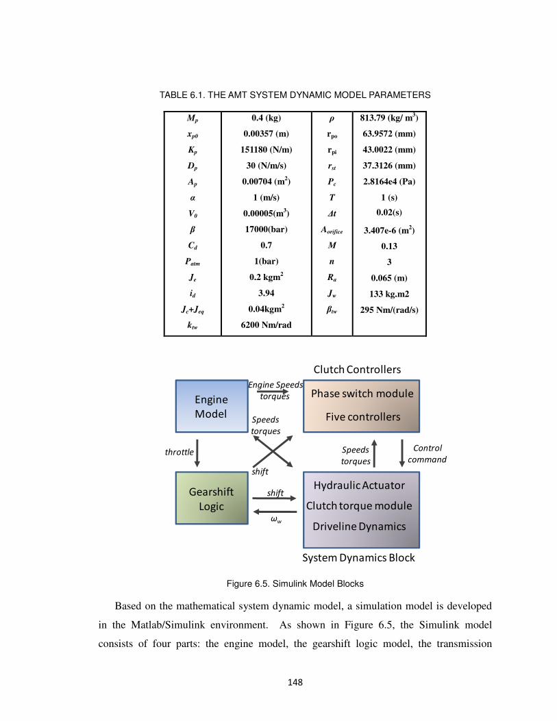
148

TABLE 6.1. THE AMT SYSTEM DYNAMIC MODEL PARAMETERS

Engine

Model

Gearshift

Logic

Clutch Controllers

System Dynamics Block

Hydraulic Actuator

Clutch torque module

Driveline Dynamics

Phase switch module

Five controllers

ωw

shift

Control

commandSpeeds

torques

Engine Speeds

torques

throttle

shift

Speeds

torques

Figure 6.5. Simulink Model Blocks

Based on the mathematical system dynamic model, a simulation model is developed

in the Matlab/Simulink environment. As shown in Figure 6.5, the Simulink model

consists of four parts: the engine model, the gearshift logic model, the transmission

Mp

xp0

Kp

Dp

Ap

α

V0

β

Cd

Patm

Je

id

Jc+Jeq

ktw

0.4 (kg)

0.00357 (m)

151180 (N/m)

30 (N/m/s)

0.00704 (m2)

1 (m/s)

0.00005(m3)

17000(bar)

0.7

1(bar)

0.2 kgm2

3.94

0.04kgm2

6200 Nm/rad

ρ

rpo

rpi

rst

Pc

T

∆t

Aorifice

Μ

n

Ra

Jw

βtw

813.79 (kg/ m3)

63.9572 (mm)

43.0022 (mm)

37.3126 (mm)

2.8164e4 (Pa)

1 (s)

0.02(s)

3.407e-6 (m2)

0.13

3

0.065 (m)

133 kg.m2

295 Nm/(rad/s)

149

driveline model, and the transmission controller model.

The engine model provides the engine speed and torque based on the input throttle.

The engine torque in the simulation is obtained from the pre-calibrated engine map,

which is interpolated from a series of discrete throttle values and engine speed values.

The gearshift logic is programmed using the Stateflow in the Simulink, and is

obtained based on the gearshift scheduling map, which provides the optimal gearshift

schedule based upon the current vehicle speed and throttle. Once the gearshift command

is initiated from the gearshift logic model, the clutch controller is triggered.

The clutch controllers include the engagement controller, the slipping opening

controller, the synchronization controller, the go-to-slipping controller, and the slipping

closing controller. The controllers switch between each other by triggering the proper

controller in the specific operating phase. When no gearshift is requested, the

engagement controller maintains a high pressure control signal to the hydraulic actuator

to maintain the clutch engagement. Once the gearshift becomes active, the clutch control

switches to the slipping opening controller and followed gearshift clutch controllers.

This control sequence is carried out in our Simulink strategy by selecting the operating

period right after the gearshift for different controllers and detecting the specific time

period. On the one hand, the “detect change” function block in the Simulink is used to

capture the gearshift request event. The starting time of the gearshift event ts is recorded.

On the other hand, the controller switching module implemented in the Simulink keeps

updating the difference tc - ts between the current time tc and ts. As shown in Figure 6.6,

when tc - ts is between 0 and 0.2 second, the slipping opening controller is activated and

the input pressure control signal to the hydraulic actuator decreases to disengage the

clutches. When tc - ts is greater than 0.2 and less than 0.4, the synchronization controller

is triggered. When tc - ts is greater than or equal to 0.4 and less than 1.1, the controller

switches to the go-to-slipping and then the slipping closing controller to engage the

clutches. When tc - ts is greater than or equal to 1.1, the engagement controller is again

activated to maintain the clutch engagement. In the future, if the new gearshift is

requested, the starting time ts is reset and the sequence repeats. As discussed before the

hydraulic pressure controller implemented in Simulink is a combination of feedforward

150

and PID controllers.

The control signals generated from the AMT controller are then sent to the AMT

transmission and the driveline system model block. This block is composed of the

hydraulic clutch actuator dynamics model, the clutch torque physics module, and the

driveline dynamics model. The clutch torque determination module simulates the clutch

torque physical characteristic. The clutch torque is the sliding friction torque when the

clutches are slipping; while it becomes static friction torque when the clutches are

engaged. The clutch torque determination module will select different equations (Eq 6.1-

Eq 6.3) to describe the different friction torques. The driveline dynamics block consists

of the engagement driveline dynamics, the slipping closing dynamics and the

synchronization. Similar to the controllers, the driveline dynamics also need to switch in

different operating phases. The parts of the model that change with different AMT

operating phases are implemented based on the event-control method. For instance, the

commutation from the slipping-closing phase to the engaged phase is obtained with the

event “ωe=ωc”.

Gearshift

logic

Detect

gear ratio

change at time ts

Gear ratio ts

If 0< tc- ts <0.2 slipping open control

If 0.2< tc- ts <0.4 synchronization control

If 0.4< tc- ts <1.1 slipping close control

If tc- ts >1.1 engagement control

Figure 6.6. Controller Switch Logic

Figure 6.7 shows the engine throttle input and the gearshift scheduling for the

simulation example. Figure 6.8 shows the corresponding simulation results. The gear

ratio is shifted from 1 to 2, and later from 2 to 3. During each gearshift, the clutch torque

first drops down to zero, and then stays for a while and finally goes up. The gearshift is

realized when there is no clutch torque transferred. And the vehicle speed continuously

increases.

151

0 2 4 6 8 10 12 14 16 18 200

20

40

thro

ttle

time (sec)

0 2 4 6 8 10 12 14 16 18 201

2

3

Gears

hift

ratio

Figure 6.7. The throttle input and gearshift scheduling

We also conducted the simulation to obtain the optimal torque trajectory using the

dynamic programming. The optimal velocity and the optimal torque trajectories are also

compared with those obtained from the feedforward and PID control results in the

Simulink simulation. To make a fair comparison, the initial conditions ωe_initial and

ωc_initial, which are defined as the speeds after synchronization and right before

engagement, of both the optimal engagement and non-optimal engagement are the same.

In addition, both of the engagements can be realized within the same time period. The

gearshift is from gear 1 to 2. The simulation only shows the clutch synchronization and

engagement process, which starts from the end of clutch disengagement and ends once

the clutch plates are engaged. Figure 6.9 shows the trajectory of the clutch velocity ωc

and the engine velocity ωe. The first 0.2 second is the synchronization phase. During the

gear synchronization, the clutch plates are totally disengaged, and therefore no clutch

torque Tc is transferred. The clutch velocity ωc is dragged down by the driveline inertia

during synchronization. On the other hand, the engine torque is assumed to be close to

zero during synchronization, and the engine velocity ωe does not change much during

synchronization. Therefore the initial speed difference before the clutch engagement

ωe_initial-ωc_initial is larger than zero. During the clutch engagement phase, the clutch

velocity does not change much due to the heavy inertia of the vehicle body, but the

engine velocity ωe decreases until the clutches are fully engaged. Figure 6.10 shows the

152

speed difference ωe-ωc. For the optimal engagement obtained from DP, the speed

difference decreases during the clutch engagement. At the final time, the change of the

speed difference becomes smaller as the derivative of ωe is constrained to be close to that

of ωc near final time of the clutch engagement. Figure 6.11 shows the clutch torque Tc

during the clutch engagement. Both of the clutch torque trajectories start from zero Nm.

For the optimal clutch torque trajectory, the maximum torque difference in each step is

limited to be smaller than 20 Nm. Figure 6.12 exhibits the engine torque Te. The engine

torque obtained from DP is required to be negative at the start of the clutch engagement,

because otherwise the engine velocity will go up. The energy loss is compared in Figure

6.13. The energy loss trajectory shows the energy lost from the initial time to the current

time t1:

1

10

( ) ( ( ) ( )) ( )t

d e c cE t t t T t dtω ω= −∫ (6.15)

We can see that at the end of the clutch engagement, the energy loss of the

engagement using DP is almost half of the one produced by the PID controller.

Therefore, to reduce energy loss, it is desirable to track the torque trajectories obtained

from the Dynamic Programming. However, the computational throughput and lack of

control means to precisely track the optimal trajectory make it difficult to be

implemented into the current Simulink model. Our future research work will be focused

on further reducing the computational throughput of the PD algorithm and developing

effective control tools to track the optimal torque trajectories from DP.

153

0 2 4 6 8 10 12 14 16 18 200

100

200

300The clutch torque (Nm)

time (sec)

clu

tch t

orq

ue (

Nm

)

0 2 4 6 8 10 12 14 16 18 20-1000

0

1000

2000

3000The clutch rotational speed

time (sec)

clu

tch s

peed (

RP

M)

0 2 4 6 8 10 12 14 16 18 200

50

100

150The engine torque

time (sec)

engin

e t

orq

ue (

Nm

)

0 2 4 6 8 10 12 14 16 18 200

10

20

30

40The vehicle speed (mph)

time (sec)

vehic

le s

peed (

mph)

Figure 6.8. The AMT simulation results

154

0 0.1 0.2 0.3 0.4 0.5 0.6 0.7 0.8320

340

360

380

400

420

440

460

480

500

time (sec)

We &

Wc (

rad/s

ec)

non-optimal

From DP

Figure 6.9. Trajectories of ωc and ωe

0 0.1 0.2 0.3 0.4 0.5 0.6 0.7 0.8-20

0

20

40

60

80

100

120

140

160

time (sec)

We-W

c (

rad/s

ec)

non-optimal

From DP

Figure 6.10. Optimal trajectory of ωe – ωc

ωe

ωc

155

0 0.1 0.2 0.3 0.4 0.5 0.6 0.7 0.80

50

100

150

200

250

time (sec)

Tc (

Nm

)

non-optimal

From DP

Figure 6.11. Optimal trajectory of Tc

0 0.1 0.2 0.3 0.4 0.5 0.6 0.7 0.8-60

-40

-20

0

20

40

60

80

100

120

140

time (sec)

Te (

Nm

)

non-optimal

From DP

Figure 6.12. Optimal trajectory of Te

156

0 0.1 0.2 0.3 0.4 0.5 0.6 0.7 0.80

1000

2000

3000

4000

5000

6000The energy loss comparison Tc x (We-Wc)

time (sec)

Energ

y loss (

Joule

)

non-optimal

From DP

Figure 6.13. Energy loss comparison

6.5. Conclusion

This chapter presents a practical Simulink dynamic model with proper complexity for

the AMT system. This AMT model provides adequate performance for AMT control

development and validation. This is also a necessity for the rapid prototyping of an AMT

controller. The developed AMT dynamic model also includes the driveline model, the

engine model, the dry clutch and the hydraulic actuator models. An AMT gearshift

control strategy is also developed that includes the gearshift control logic and the clutch

control methodology. The developed AMT dynamic model and controller are realized in

Simulink. Simulation validation results show that the developed AMT model, along with

its controller, provides adequate complexity for control system simulation and

development with proper throughput for real-time simulation. In addition, to realize an

energy efficient and smooth clutch engagement, the dynamic programming method is

used to generate the optimal clutch and engine torque control and it shows an almost 50%

energy saving during the clutch engagement.

157


[1] Sun, Z. and Hebbale, K., “Challenges and opportunities in automotive transmission

control”, Proceedings of 2005 American Control Conference, Portland, OR, pp. 3284-

3289, June 8-10, 2005.

[2] Glielmo, L. Iannelli, L. Vacca, V. and Vasca, F. “Gearshift Control for Automated

Manual Transmissions”, IEEE/ASME Transactions on Mechatronics, VOL 11, No. 1,

Feb., 2006.

[3] F. Garofalo, L. Glielmo, L. Iannelli, and F. Vasca, “Smooth engagement for

automotive dry clutch” in Proc. 40th IEEE Conf. Decision and Control, Orlando, FL,

2001, pp. 529-534

[4] F. Amisano, G. Serra, and M. Velardocchia, “Engine control strategy to optimize a

shift transient during clutch engagement,” SAE Tech. Paper Series, no. 2001-01-0877, pp.

115–120, 2001.

[5] K. Hayashi, Y. Shimizu, S. Nakamura, Y. Dote, A. Takayama, and A. Hirako, “Neuro

fuzzy optimal transmission control for automobile with variable loads,” in Proc. IEEE

Industrial Electronics, Control, and Instrumentation Conf., Maui, HI, 1993, vol. 1, pp.

430–434

[7] L. Glielmo, L. and F. Vasca, “Engagement Control for Automotive Dry Clutch”,

Proceedings of 2000 American Control Conference, Chicago, Illinois, pp. 1016-1017,

June, 2000.

[8] Bellman, R., Dynamic Programming, Princeton University Press, New Jersey, 1957.

[9] Bellman, R. and Dreyfus, S., Applied Dynamic Programming, Princeton University

Press, New Jersey, 1962.

[10] Bertsekas, D., Dynamic Programming and Optimal Control, Athena Scientific, 1995.


Using A Customized Dynamic Programming Method”. Proceedings of the 2008 ASME

Dynamic System and Control Conference, DSC2008-2166, Ann Arbor, Michigan, 2008.

[12] H. Meritt, Hydraulic Control Systems, New York: Wiley, 1967.

158

[13] Luigi Glielmo , Luigi Iannelli, Vladimiro Vacca, Francesco Vasca, “Speed Control

for Automated Manual Transmission with Dry Clutch”, 43rd IEEE Conference on

Decision and Control, 1709—1714, Atlantis, Paradise Island, Bahamas, December 14-17,

2004

[14] http://www.adi.com/products_emu_pci.htm, 2009

[15] L. Glielmo and F. Vasca, “Optimal control of dry clutch engagement,” SAE Trans., J.

Passenger Cars: Mech. Syst., vol. 6, no. 2000-01-0837, 2000.

[16] J. Slicker and R. N. K. Loh, “Design of robust vehicle launch control system,” IEEE

Trans. Contr. Syst. Technol., vol. 4, no. 4, pp. 326–335, Jul. 1996.

[17] A. Bemporad, F. Borrelli, L. Glielmo, and F. Vasca, “Hybrid control of dry clutch

engagement,” in Proc. European Control Conf., Porto, Portugal, 2001.

[18] H. Tanaka and H. Wada, “Fuzzy control of clutch engagement for automated manual

transmission,” Veh. Syst. Dyn., vol. 24, pp. 365–376, 1995.

[19] Y. Lei, M. Niu, and A. Ge, “A research on starting control strategy of vehicle with

AMT,” in Proc. FISITA World Automotive Congress, Seoul, Korea, 2000.

[20] A. Szadkowski and R. B. Morford, “Clutch engagement simulation: Engagement

without throttle,” SAE Tech. Paper Series, no. 920766, 1992.

[21] J. Fredriksson and B. Egardt, “Nonlinear control applied to gearshifting in

automated manual transmission,” in Proc. 39th IEEE Conf. Decision and Control,

Sydney, Australia, 2000, pp. 444–449.

[22] F. Amisano, R. Flora, and M. Velardocchia, “A linear thermal model for an

automotive clutch,” SAE Tech. Paper Series, no. 2000-01-0834, 2000.

[23] D. Centea, H. Rahnejat, and M. T. Menday, “The influence of the interface

coefficient of friction upon the propensity to judder in automotive clutches,” Proc. Inst.

Mech. Eng., vol. 213, pt. D, pp. 245–268, 1999.

[24] E. M. A. Rabeih and D. A. Crolla, “Intelligent control of clutch judder and shunt

phenomena in vehicle drivelines,” Int. J. Veh. Des., vol. 17, no. 3, pp. 318–332, 1996

159

[25] DeLaSalle, S., Jansz, M., and Light, D. (1999), Design of a Feedback Control

System for Damping of Vehicle Shuffle. Proceedings of the EAEC Conference,

Barcelona, pp 278–284.

[26] Mo, C.Y., Beaumount, A.J., and Powell, N.N. (1996), SAE 960046, Active Control

of driveability, pp 215–221.

[27] Baumann, J., Torkzadeh, D.D., Ramstein, A., Kienke, U., and Schelegl, Model-based

predictive anti-jerk control T. Control Engineering Practice, 14, 259–266 (2006).

[28] Balfour, G., Dupraz, P., Ramsbottom, M., and Scotson, Diesel fuel injection control

for optimum driveability SAE 2000-01-0265.

160

Chapter 7

The Propulsion System Level Design--Tracking Control of

Periodic Signals with Varying Magnitude and Its Application

To Hybrid Powertrain

A successful power transmission design should not only be able to operate

efficiently and smoothly itself, but more importantly, it should also enable the power

source energy efficient operation and reject the potential driveline vibration triggered by

the power source. To be specific, the aggressive energy management of the hybrid

powertrain and the HCCI combustion introduced previously both require a power

transmission mechanism with efficient vibration rejection capability. As indicated in

Chapter 1, vibration is one of the most difficult and important issue for propulsion and

power transfer. In this thesis, we will propose control framework, which is expected to

be effective solution for the energy efficient vibration reduction for a class of propulsion

and power transfer system involving rotational motion. This framework will be explained

based on the hybrid vehicle power train vibration reduction problem.

7.1. Introduction

The problem of tracking or rejecting signals generated by exogenous systems (exo-

system) has been widely investigated and applied by researchers. One of the important

research outcome for linear time invariant system is the internal model principle [1-2],

which indicates that any feedback controller capable of tracking/ rejecting the specific

signal/disturbance must embed a proper copy of the exo-system into the controller

design. The problem in nonlinear setting is investigated in [3], and recent research work

[4,5,6] explores the theory for linear time varying systems.

Based on the internal model principle, the repetitive controller [7] was proposed

mainly for periodic signal tracking/rejection with only the period known. A delay with a

positive feedback is embedded as an internal model in the repetitive control design. To

enable real-world applications, the zero phase compensation [8] mechanism was

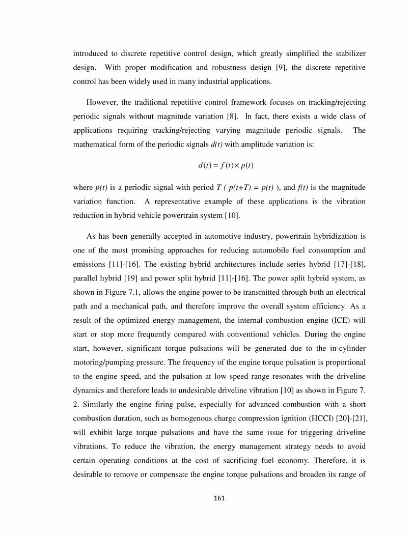
161

introduced to discrete repetitive control design, which greatly simplified the stabilizer

design. With proper modification and robustness design [9], the discrete repetitive

control has been widely used in many industrial applications.

However, the traditional repetitive control framework focuses on tracking/rejecting

periodic signals without magnitude variation [8]. In fact, there exists a wide class of

applications requiring tracking/rejecting varying magnitude periodic signals. The

mathematical form of the periodic signals d(t) with amplitude variation is:

( ) ( ) ( )d t f t p t= ×

where p(t) is a periodic signal with period T ( p(t+T) = p(t) ), and f(t) is the magnitude

variation function. A representative example of these applications is the vibration

reduction in hybrid vehicle powertrain system [10].

As has been generally accepted in automotive industry, powertrain hybridization is

one of the most promising approaches for reducing automobile fuel consumption and

emissions [11]-[16]. The existing hybrid architectures include series hybrid [17]-[18],

parallel hybrid [19] and power split hybrid [11]-[16]. The power split hybrid system, as

shown in Figure 7.1, allows the engine power to be transmitted through both an electrical

path and a mechanical path, and therefore improve the overall system efficiency. As a

result of the optimized energy management, the internal combustion engine (ICE) will

start or stop more frequently compared with conventional vehicles. During the engine

start, however, significant torque pulsations will be generated due to the in-cylinder

motoring/pumping pressure. The frequency of the engine torque pulsation is proportional

to the engine speed, and the pulsation at low speed range resonates with the driveline

dynamics and therefore leads to undesirable driveline vibration [10] as shown in Figure 7.

2. Similarly the engine firing pulse, especially for advanced combustion with a short

combustion duration, such as homogenous charge compression ignition (HCCI) [20]-[21],

will exhibit large torque pulsations and have the same issue for triggering driveline

vibrations. To reduce the vibration, the energy management strategy needs to avoid

certain operating conditions at the cost of sacrificing fuel economy. Therefore, it is

desirable to remove or compensate the engine torque pulsations and broaden its range of

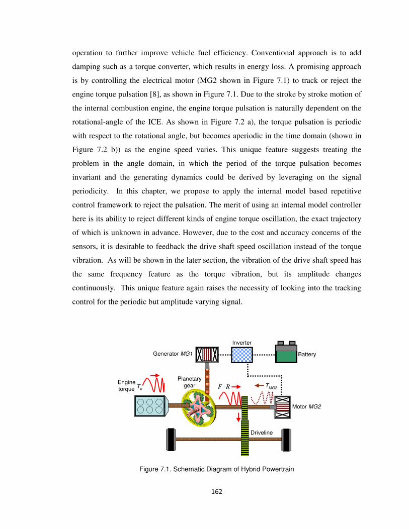
162

operation to further improve vehicle fuel efficiency. Conventional approach is to add

damping such as a torque converter, which results in energy loss. A promising approach

is by controlling the electrical motor (MG2 shown in Figure 7.1) to track or reject the

engine torque pulsation [8], as shown in Figure 7.1. Due to the stroke by stroke motion of

the internal combustion engine, the engine torque pulsation is naturally dependent on the

rotational-angle of the ICE. As shown in Figure 7.2 a), the torque pulsation is periodic

with respect to the rotational angle, but becomes aperiodic in the time domain (shown in

Figure 7.2 b)) as the engine speed varies. This unique feature suggests treating the

problem in the angle domain, in which the period of the torque pulsation becomes

invariant and the generating dynamics could be derived by leveraging on the signal

periodicity. In this chapter, we propose to apply the internal model based repetitive

control framework to reject the pulsation. The merit of using an internal model controller

here is its ability to reject different kinds of engine torque oscillation, the exact trajectory

of which is unknown in advance. However, due to the cost and accuracy concerns of the

sensors, it is desirable to feedback the drive shaft speed oscillation instead of the torque

vibration. As will be shown in the later section, the vibration of the drive shaft speed has

the same frequency feature as the torque vibration, but its amplitude changes

continuously. This unique feature again raises the necessity of looking into the tracking

control for the periodic but amplitude varying signal.

TeTMG2RF ⋅

Engine torque

Generator MG1

Motor MG2

Battery

Inverter

Driveline

Planetary

gear

Figure 7.1. Schematic Diagram of Hybrid Powertrain

163

As will be revealed in the following section, the generating dynamics of the

magnitude varying periodic signal could be time varying, instead of being time invariant

as those for purely periodic signal. Thus the traditional repetitive control design

mechanism, which mainly treats time invariant generating dynamics, will not ensure

asymptotic tracking performance. Therefore, a new framework for controlling magnitude

varying periodic signals needs to be developed. More interestingly, in the hybrid

powertrain problem, the magnitude variation for the velocity oscillation to be rejected is

due to the integration of the torque vibration with varying frequency, and thus its

generating dynamics needs to be specially derived. Furthermore, as will be shown in this

chapter, as the hybrid powertrain vibration problem is treated in the angle domain to gain

the signal periodicity, the actuator plant dynamics need to be converted to the angle

domain as well, which will result in a time varying (actually angle varying) plant

dynamics.

0 50 100 150 200 250 300 350 400 450-100

-50

0

50

100

Rotational angle (deg)

a)

Engin

e T

orq

ue (

Nm

)

0 0.1 0.2 0.3 0.4 0.5 0.6 0.7 0.8-100

-50

0

50

100

Time (sec)

b)

Engin

e T

orq

ue (

Nm

)

Figure 7.2. Engine Torque Oscillation in Time and Angle Domain

To sum up, the problem defined above is the tracking/rejection control of a

magnitude varying periodic signal/disturbance with a time varying plant dynamics.

Interestingly, together with the generating dynamics and the control framework presented

in this chapter, our recently developed time varying repetitive control design method [4]

164

provides an effective tool to solve the above defined problem. The rest of this chapter is

organized as follows. Section 7.2 analyzes the generating dynamics for periodic signal

with amplitude variation. Section 7.3 formulates the hybrid powertrain vibration

reduction problem as a amplitude changing periodic disturbance rejection problem.

Section 7.4 presents the controller design for the hybrid vehicle vibration reduction.

Section 7.5 shows the controller design process and the simulation results. Conclusion is

provided in section 7.6.

7.2. Tracking Control of Periodic Signal with Time-Varying Amplitude

In this section, we will analyze the generating dynamics of the periodic signals with

amplitude change, where the period T and the magnitude variation are known a priori. It

is well known from Fourier series that the periodic signal p(t) with period T can be

expressed by infinite combinations of harmonic signals, and therefore the finite order

polynomial can not generate such p(t). But in discrete time, by taking advantage of the

periodicity [6],

( ) ( )p k p k N= − (7.1)

where k is the current discrete time step, N=T/∆t is the discrete time period and ∆t is the

sampling time internal.

The generating dynamics can therefore be written as:

( ) 1 Nz z

−Λ = − (7.2)

with the left-shift operator z, ie. z[p](k)=p(k+1).

Following the similar approach, we can also derive the discrete generating dynamics

for the magnitude varying periodic signal d(t).

Theorem 7.1. If the amplitude change of the periodic signal follows a trajectory

describing by f(t), where t is the time variable, then the discrete generating dynamics of

this signal will be:

165

( )( ) 1

( )

N f k Nz z

f k

− +Λ = − (7.3)

Proof: The periodicity of the signal yields

( ) ( )

( ) ( )

Nd k d k z

f k f k N

−

=−

(7.4)

then we can have

( )[1 ] ( ) 0

( )

Nf k z

d kf k N

−

− =−

(7.5)

which yields

( )[1 ] ( ) 0

( )

N f k Nz d k

f k

− +− = (7.6)

therefore the generating dynamics will be

( )( ) 1

( )

N f k Nz z

f k

− +Λ = − (7.7) ■

The generating dynamics (7.3) is time varying, as f(k+N)/f(k) is not constant. Figure

7.3 shows the commonly used internal model controller structure in repetitive control,

where A-1

B is the plant model, and the feedback loop formed by PQ-1

and G-1

F is the

internal model controller. In the discrete repetitive control [6] for linear time invariant

plant, PQ-1

is z-N

, and G-1

F is 1, thus the feedback internal model controller will be

exactly the generating dynamics (7.2). However, in case of the time varying generating

dynamics (7.7), directly embedding the generating dynamics (7.7) by

assigning 1 ( )

( )

N f k NPQ z

f k

− − += and G

-1F as 1 will not yield asymptotic performance, even if

the plant A-1

B is linear time invariant. The fundamental reason is due to the time varying

PQ-1

. This argument can be better explained by the following lemma [4]:

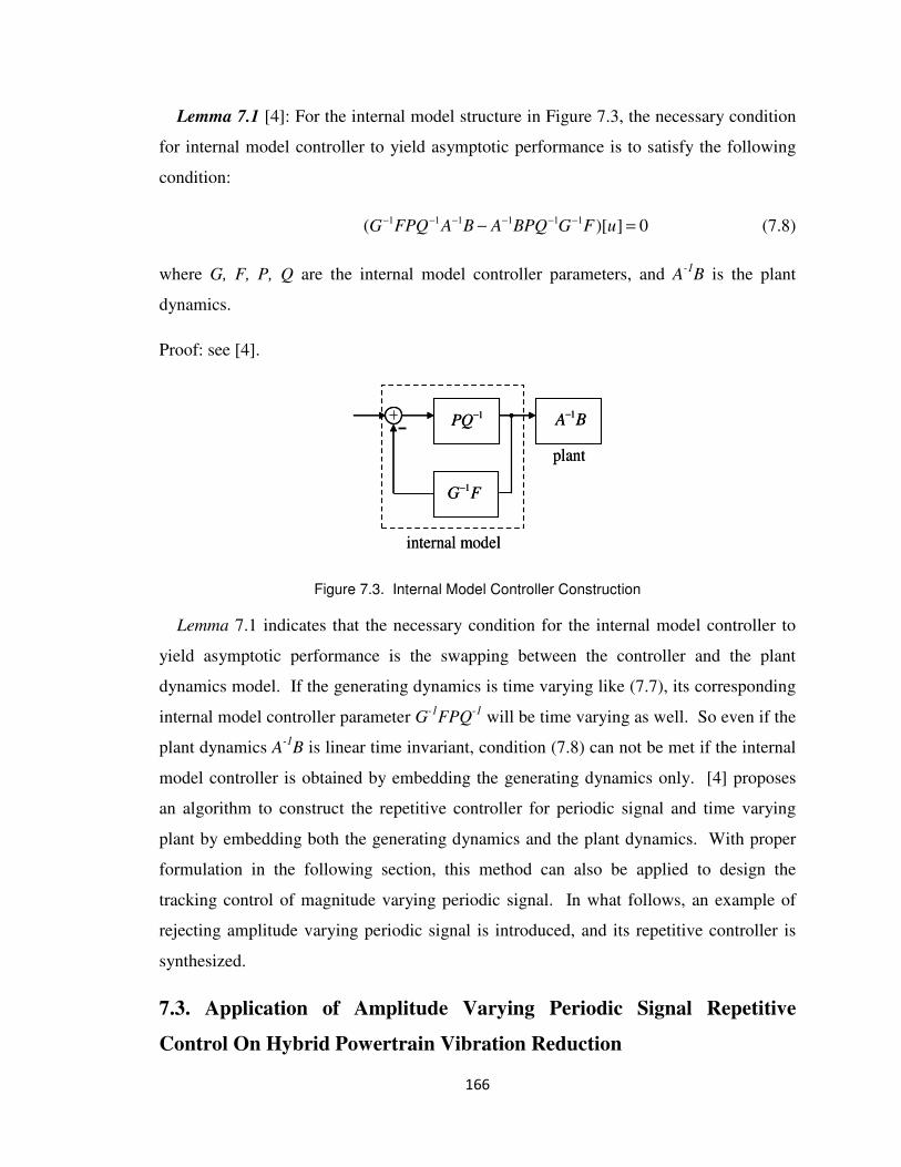
166

Lemma 7.1 [4]: For the internal model structure in Figure 7.3, the necessary condition

for internal model controller to yield asymptotic performance is to satisfy the following

condition:

1 1 1 1 1 1( )[ ] 0G FPQ A B A BPQ G F u− − − − − −− = (7.8)

where G, F, P, Q are the internal model controller parameters, and A-1

B is the plant

dynamics.

Proof: see [4].

1PQ

− 1A B

−

1G F

−

plant

internal model

1PQ

− 1A B

−

1G F

−

plant

internal model

Figure 7.3. Internal Model Controller Construction

Lemma 7.1 indicates that the necessary condition for the internal model controller to

yield asymptotic performance is the swapping between the controller and the plant

dynamics model. If the generating dynamics is time varying like (7.7), its corresponding

internal model controller parameter G-1

FPQ-1

will be time varying as well. So even if the

plant dynamics A-1

B is linear time invariant, condition (7.8) can not be met if the internal

model controller is obtained by embedding the generating dynamics only. [4] proposes

an algorithm to construct the repetitive controller for periodic signal and time varying

plant by embedding both the generating dynamics and the plant dynamics. With proper

formulation in the following section, this method can also be applied to design the

tracking control of magnitude varying periodic signal. In what follows, an example of

rejecting amplitude varying periodic signal is introduced, and its repetitive controller is

synthesized.

7.3. Application of Amplitude Varying Periodic Signal Repetitive

Control On Hybrid Powertrain Vibration Reduction

167

In this section, the hybrid powertrain dynamics and its vibration caused by engine

starting and stopping is analyzed. The vibration signal to reject is shown to be periodic

with varying amplitude. The generating dynamics is then derived and the appropriate

controller design method will be discussed.

7.3.1 Formulation of the Vibration Rejection Problem

Engine

Dynamics

Hybrid Transmission

Dynamics

Generator Dynamics (MG1)

Driveline

Dynamics

Motor

(MG2)

Vehicle

acceleration

)(

)(

)(

1

111

SRSR

RFSFTII

TSFII

eMGr

ecee

MGsMGMG

+=+

⋅−⋅−=+

−⋅=+

ωωω

ω

ω

��

�

�

Te

TMG1 TMG2

RF ⋅

Resistance Torque Tres

Figure 7.4. Block Diagram of the Hybrid System

Figure 7.4 shows the block diagram of the hybrid powertrain system in Figure 7.1.

During the engine start, significant torque pulsations will be generated due to the in-

cylinder motoring/pumping pressure. As shown in Figure 7.4, the engine torque Te and

the generator (MG1) torque TMG1 are combined through a hybrid transmission planetary

gear set, which outputs the torque F·R. The torque F·R, together with the motor torque

TMG2, is the input to the vehicle driveline. The hybrid powertrain dynamics is shown as

the following [11]:

1 1 1

2

2 2

( )

( )

( ) ( )

MG MG s MG

e e c e

tire

r MG r MG res

I I F S T

I I T F S F R

Rm I K I K T F R K T

K

ω

ω

ω

+ = ⋅ −

+ = − ⋅ − ⋅

+ + = + ⋅ −

�

�

�

(7.9)

where 1MGω ,

eω ,

rω are the rotational speed of the motor MG1, the engine, and the

ring gear [13] respectively, and here we assume the ring gear speed r

ω is equal to the

drive shaft rotational speed. Ir, Is and Ic are the inertias of the ring gear, the sun gear and

the carrier gear. IMG1, IMG2 and Ie are the inertias of the motor MG1, motor MG2 and the

168

engine respectively. F is the internal force on the pinion gear and m is the vehicle mass.

K is the final driven ratio, and Tres is driveline and wheel resistance torque.

Equation (7.9) indicates that, the planetary gear set based hybrid transmission adds

the flexibility [11] of power management of the engine and generator/motor, but directly

transfers the engine torque Te to the driveline without vibration damping in between [8].

The engine torque pulsation due to the pumping pressure will be directly transferred to

the driveline, and will result in driveline vibration [8]. This problem becomes severe at

low engine speed. First, the frequency of the engine torque pulsation is proportional to

the engine speed, and the low oscillating frequency at low engine speed resonates with

the driveline dynamics. Second, the engine motoring during engine starting will generate

larger engine torque pulsation than its normal operation, and therefore will cause

significant driveline vibration. However, the low speed engine operation is inevitable. In

hybrid vehicles, engine starting and stopping should occur frequently to switch power

sources and therefore provide better fuel economy. The Toyota Automotive research

group [8] unveiled this problem in Toyota Prius hybrid powertrain, and their proposed

solution is to control the motor torque in an open loop fashion to compensate the

vibration, which is certainly not the most effective way.

Engine

Dynamics

Hybrid

Transmission

Dynamics

Generator

Dynamics (MG1)

Driveline

Dynamics

Motor

(MG2)

Te

TMG2

TMG2

),(),(1

tsMtsN−

),(),(1

tsQtsP−

),(),(1

tsFtsG−

Internal Model

Tres

Stabilizer

Driveshaft speed

rω

Figure 7.5. Control Block Diagram for vibration reduction

169

0 1 2 3 4 50

200

400

time (second)

engin

e s

peed

(rp

m)

0 1 2 3 4 5-100

0

100

time (second)

eng

ine t

orq

ue (

Nm

)

0 1 2 3 4 50

2

4

time (second)

Velo

city

osc

illa

tion

(ra

d/s

ec)

0 200 400 600 800 1000 1200 1400 16000

2

4

angle (degree)

Velo

city

osc

illa

tio

n (

rad/s

ec)

Figure 7.6. Magnitude Varying Periodic Velocity Variation

In this chapter, we propose to reject the disturbance with an internal model controller.

Interestingly, due to the stroke by stroke motion of the internal combustion engine, the

engine torque pulsation is naturally dependent of the rotational-angle θ of the ICE. As

shown in Figure 7.2 a), the torque pulsation is periodic with respect to the engine

rotational angle θ, but becomes aperiodic in the time domain (shown in Figure 7.2 b)) as

the engine speed varies. While it is generally difficult to derive the generating dynamics

for an arbitrary aperiodic signal, this unique feature suggests treating the problem in the

angle domain, in which we can take advantage of the periodicity to obtain the generating

dynamics. Since in practice the torque oscillation is difficult to measure and note that the

torque pulsation results in speed vibration, we use the drive shaft rotational speed as the

feedback control variable as shown in Figure 7.5. The speed vibration, which is

mathematically the integration of the torque pulsation, is still aperiodic in the time

domain. But different from the torque pulsation, it is periodic with varying magnitude in

the angle domain. This fact can be better illustrated by Figure 7.6. As the frequency of

170

the acceleration A becomes higher and higher, the magnitude of the velocity V becomes

smaller. The mathematical meaning is that the integration of the signal with varying

frequency decreases as the frequency goes up. To construct the internal model controller,

we first need to derive its generating dynamics of the velocity oscillation signal.

Theorem 7.2: If dV

Adt

= , and A is periodic with respect to the rotational angle but

aperiodic with respect to time, then the discrete generating dynamics in the angle domain

for signal V is

1 ( 1)( ) ( 1)( , ) 1

( ) ( 1)

N Ne e

e e

k kz k z z z

k N k N

ω ω

ω ω− − − + +

Λ = − − ++ + +

(7.10)

where N is the period of the discrete periodic signal A in the angle domain.

Proof: Noting that dV

Adt

= , which implies:

( )dV dA

d dt

θ θ

θ= , (7.11)

where θ is the engine rotational angle. As

( )e

d

dt

θω θ= (7.12)

Substitute Eq.(7.12) to equation (7.11) yields

( )( )

e

dVA

d

θω θ

θ= (7.13)

As A is periodic in the rotational angle domain, ( )

( )e

dV

d

θω θ

θ is periodic with

respect to θ as well. Therefore,

( ) ( )( ) ( )

e e

dV k dV k Nk k N

d dω ω

θ θ

−= − (7.14)

Replacing the derivative term in Eq.(14) by discrete approximation yields

171

1 1( ) ( ) ( ) ( )N

e e

z zk V k z k V k

z zω ω

θ θ−− −

=∆ ∆

(7.15)

After proper transformation, we can get

1 1( ) ( ) ( ) ( )N

e e

z zk V k z k V k

z zω ω

θ θ−− −

=∆ ∆

(7.16)

which yields

1 ( 1)( ) ( 1)[1 ] ( ) 0

( ) ( 1)

N Ne e

e e

k kz z z V k

k N k N

ω ω

ω ω− − − + +

− − + =+ + +

■

Remark: Note that the sampling step k corresponds to each sampling instant of θ,

instead of time t. N is the number of sampling times in one period. ωe is the engine

rotational speed. Also note that the generating dynamics depends on the engine rotational

speed ωe. As the speed ωe is changing with time, the generating dynamics (7.10) is

actually time varying (actually angle varying, but in this chapter we do not specifically

discriminate these two terminologies). In addition, the order of the generating dynamics

is N+1, which is one order higher than the signal sampling rate per period cycle.

7.4. Rotational Angle Based Control

As generating dynamics of the vibration signal is derived in the angle domain, the

actuator dynamics needs to be converted to the angle domain as well. In this section, we

will show the construction of the actuator dynamics in the angle domain.

7.4.1 Plant Dynamics Model

As analyzed in section 7.3, the drive shaft rotational velocity is fed back to form the

feedback loop as shown in Figure 7.5.

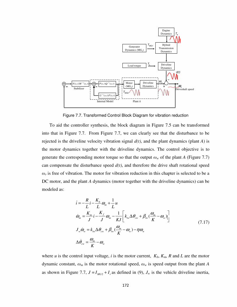
172

Engine

Dynamics

Hybrid

Transmission

Dynamics

Generator

Dynamics (MG1)

Driveline

Dynamics

Motor

(MG2)

Te

TMG1

TMG2

),(),(1

tsMtsN−

),(),(1

tsQtsP−

),(),(1tsFtsG

−

Internal Model

Driveline

Dynamics

Plant A

Driveshaft speedStabilizer

Load torqueTL

d(t)

rω

rω

wω

Figure 7.7. Transformed Control Block Diagram for vibration reduction

To aid the controller synthesis, the block diagram in Figure 7.5 can be transformed

into that in Figure 7.7. From Figure 7.7, we can clearly see that the disturbance to be

rejected is the driveline velocity vibration signal d(t), and the plant dynamics (plant A) is

the motor dynamics together with the driveline dynamics. The control objective is to

generate the corresponding motor torque so that the output ωw of the plant A (Figure 7.7)

can compensate the disturbance speed d(t), and therefore the drive shaft rotational speed

ωr is free of vibration. The motor for vibration reduction in this chapter is selected to be a

DC motor, and the plant A dynamics (motor together with the driveline dynamics) can be

modeled as:

1

1( )

( )

b

m

fm m

m m tw cw tw w

m

w w tw cw tw w w

m

cw w

KRi i u

L L L

KKi k

J J KJ K

J kK

K

ω

ωω ω θ β ω

ωω θ β ω ηω

ωθ ω

= − − +

= − − ∆ + −

= ∆ + − −

∆ = −

�

�

�

�

(7.17)

where u is the control input voltage, i is the motor current, Kb, Km, R and L are the motor

dynamic constant, ωm is the motor rotational speed, ωw is speed output from the plant A

as shown in Figure 7.7, J =2MG r

I I+ as defined in (9), Jw is the vehicle driveline inertia,

173

θcw is the driveshaft torsional angle, ktw is elastic stiffness coefficient, βtw is friction

coefficients, and η is the driveline damping coefficient. Here we assume the total

driveline resistance torque Tres is a combination of the load torque TL and the damping

torque ηωw. The load torque TL is assumed constant during the engine start/stop period

due to the short engine start/stop duration. The model can be further reduced by assuming

the rigidity of the driveline shaft and thus ωm = ωw. Therefore the dynamics model

becomes:

1

1( )

( )

b

w

w m f w w

w

KRi i u

L L L

KK i KKKJ J

ω

ω ω ηω

= − − +

= × − −+

�

�

(7.18)

Which can be translated into the state space form as :

( ) ( ) ( )

( ) ( )

( ) ( ) ( )

x t Ax t Bu t

y t Cx t

e t Cx t d t

= +

=

= +

�

(7.19)

where

( ) ( )

b

fm

w w

KR

L LA

KKKK

KJ J KJ J

η

− −

=+

− + +

,

1

0

B L

=

, 0

1C

=

, w

ix

ω

=

,

where d(t) is the disturbance to be rejected, whose generating dynamics in the angle

domain is Eq (7.10) .

7.4.2 Conversion of the Plant Model to Angle Domain

As the problem is to be investigated in the angle domain, and also because the

generating dynamics (7.10) is derived in angle domain, the plant model (7.19) should also

be converted into the rotational angle domain [4] as:

174

( ) 1 1( ) ( )

( ) ( )

( ) ( )

( ) ( ) ( )

e e

dxAx B u

d

y Cx

e Cx d

θθ θ

θ ω θ ω θ

θ θ

θ θ θ

= +

=

= +

(7.20)

Note that d is periodic with respect to the engine rotational angle θ(t) and θ(t) is

defined as 0

( ) ( )t

et

t dθ ω τ τ= ∫ . Clearly the model (7.20) is linear angle varying. In this

chapter we still call system (7.20) linear time varying system as the system remains same

if the operator θ is replaced by operator t. It can be verified that system (7.20) is

uniformly controllable and observable [4]. For implementation, it is sampled at evenly

discrete angle intervals θ(k), θ(k+1),…, and the rotational domain discrete system model

can be formed as [4]:

( 1) ( ) ( ) ( ) ( )

( ) ( ) ( ) ( )

x k F k x k G k u k

e k H k x k d k

+ = +

= + (7.21)

where k+1 denotes the sampling angle instant θ(k+1), and ( ) ( )AT

F k e k=

with 1( ) ( ( ) )

ATG k e k I A B

−= − , when matrix A is non-singular.

7.4.3 Internal Model Controller Design

In order to apply our recently developed controller design [4] via I/O representation,

we need to transform the state space model (7.21) to polynomial fraction representation

[20]. To do so, we briefly introduce the definitions on polynomial differential operator

(PDO) (see [20]).

Definition 7.1: Denote the one step delay operator z-1

. The left polynomial

differential operator (PDO) of degree n, P(z, k), is defined as:

1

1 0( , ) ( ) ( ) ( )n

nP z k a k z a k z a k

− −= + + +� (7.22)

where ai(k) are bounded and nonzero functions of k for k>0. If a0(k)=1 for all k, then the

above left PDO is termed as monic.

The Input/Output (I/O) representation of the discrete state space mode (7.21) can

then be derived following the method in [4] as:

175

1( ) ( , ) ( , ) ( ) ( )y k A z k B z k u k d k−= + (7.23)

Where A(z,k) and B(z,k) are two PDOs defined as (7.22).

We recall our recently developed results [4] for the time varying tracking control

design:

Proposition 1: [4] Consider plant model (7.21) and exogenous signal model (7.10).

The controller structure is shown in Figure 7.7. Design G(z,k)=A(z,k), and F(z,k)=B(z,k).

If PDO P(z,k), Q(z,k), N(z,k) and M(z,k) satisfy the following conditions:

( , ) ( , ) ( , ) ( , ) ( , ) ( , )A z k Q z k B z k P z k z k Q z k+ = Λ (7.24)

( , ) ( , ) ( , ) ( , ) ( , ) ( , ) ( , )s

z k Q z k M z k B z k P z k N z k A z kΛ + = (7.25)

where ( , )s

A z k is exponentially stable PDO, and

1( , ) ( , ) ( , )M z k Q z k M z k−=

1( , ) ( , ) ( , )N z k Q z k N z k−=

Then the asymptotic performance is achieved, i.e., lim ( ) 0w

kkω

→∞= .

Note that M(z,k) and N(z,k) are the stabilizing controllers shown in Figure 7.7. For

more information about the controller design theory, please refer to [4].

TABLE 7. 1. PARAMETER VALUES OF THE DYNAMIC MODEL

R

L

Km

ktw

Kf

η

2 ohms

0.05 henrys

150 Nm/amp

6200 Nm/rad

0.5 Nm/(rad/s)

49.5 Nm/(rad/s)

J

Jw

βtw

Kb

Ra

K

32.9 kg.m2

133 kg.m2

295 Nm

50 V/(rad/s)

0.065 m

3.9

7.5. Simulation Results

176

In this section, we present the simulation results of applying the angle based time-

varying repetitive control together with the generating dynamics (7.10) to compensate for

the engine torque pulsation in the hybrid powertrain. The idea is to control the motor in

the hybrid powertrain to generate the appropriate torque to counteract the engine torque

pulsation so that driveline vibration can be suppressed. Heavy duty DC motor parameters

have been selected for the dynamics model for preliminary investigation as shown in

Table 1.

Due to the stroke by stroke motion, the pulsation disturbance d is periodic in the

angle domain. To precisely represent d, we use 23 samples for sampling rate per period

cycle, and therefore the generating polynomial (7.10) for the disturbance d is given by

1 23 24( ) ( 1)( , ) 1

( 23) ( 24)

e e

e e

k kz k z z z

k k

ω ω

ω ω− − − +

Λ = − − ++ +

(7.26)

Now, given the plant dynamics model (7.23) and the generating dynamics model

( , )z kΛ (7.26), The controller design follows two steps [4].

Step1: Solve P(z,k) and Q(z,k) to satisfy condition (7.24).

Setp 2: Solve ( , )M z k and ( , )N z k to meet condition (7.25).

The internal model controller in Figure 7.7 can therefore be constructed. The high

order generating polynomial (7.26) inevitably enforces the high order internal model and

stabilizing controller. The order of P(z, k)Q-1

(z, k) in the internal model unit is 23 and the

order of the stabilizer N(z,k)M-1

(z,k) is 24. The high order controller is then simulated in

Matlab/Simulink.

Finally, Figure 7.8 and Figure 7.9 show the simulation results. Here the control

target is to control the system to track the driveshaft speed oscillation. Then the

difference between the tracking result and the speed oscillation will be the output of the

disturbance rejection. Thus the better the tracking result, the smaller the oscillation will

be. Two controller design methods are compared. The first one is designed using the

traditional repetitive control internal model generating dynamics (Eq 7.10), and the

177

second controller is designed based on our approach proposed in this chapter. Figure 7.8

shows the tracking result for a smooth engine start (the engine speed increases slowly).

Figure 7.8(b) and Figure 7.8(c) compares the tracking result of magnitude varying

periodic disturbance signal (the drive shaft speed oscillation), using the traditional

repetitive control generating dynamics Eq (7.2) and that using Eq (7.10) derived in this

chapter respectively. The traditional approach does not guarantee asymptotic

performance, but the tracking error is not evident here. This is because the magnitude

change of the oscillation velocity is related to the variation rate of the engine speed. As a

slowly varying engine speed ωe (Figure 7.8(a)) results in slow magnitude change of the

driveshaft oscillation speed, the loss of tracking using the traditional repetitive control

approach is not apparent. However, Figure 7.9 shows the tracking result for a steep

engine start. Figure 7.9(b) clearly shows a significant tracking error using the traditional

repetitive control internal model generating dynamics, while the tracking result in Figure

7.9 (c) clearly exhibits the asymptotic tracking performance using our proposed controller

with the generating dynamics [10].

0 0.2 0.4 0.6 0.8 1 1.2 1.4 1.610

15

20

25

30

35

40

45

50

55

60

time (seond)

eng

ine s

pee

d (

rpm

)

Figure 7.8(a). Engine Speed Profile

178

0 0.2 0.4 0.6 0.8 1 1.2 1.4 1.6-4

-3

-2

-1

0

1

2

3

4

time (seond)

spe

ed

(ra

d/s

ec)

Disturbance

tracking result

Figure 7.8(b). Tracking Result Using the Generating Dynamics From Traditional Repetitive

Control

0 0.2 0.4 0.6 0.8 1 1.2 1.4 1.6-4

-3

-2

-1

0

1

2

3

4

time (seond)

spe

ed

(ra

d/s

ec)

Disturbance

tracking result

Figure 7.8(c). Tracking Result Using the Developed Generating Dynamics

179

0 0.2 0.4 0.6 0.8 10

50

100

150

200

250

300

350

400

time (seond)

eng

ine s

pee

d (

rpm

)

Figure 7.9 (a). Steep Engine Speed Profile

0 0.2 0.4 0.6 0.8 1-4

-3

-2

-1

0

1

2

3

4

time (seond)

spe

ed

(ra

d/s

ec)

Disturbance

tracking result

Figure 7.9(b). Tracking Result Using the Generating Dynamics From Traditional Repetitive

Control

180

0 0.2 0.4 0.6 0.8 1-4

-3

-2

-1

0

1

2

3

4

time (seond)

spe

ed

(ra

d/s

ec)

Disturbance

tracking result

Figure 7.9(c). Tracking Results Using the Developed Generating Dynamics

7.6. Conclusion

This chapter presents the tracking or rejection of periodic signals with varying peak

to peak magnitude. The generating dynamics for this kind of signals are first derived.

Moreover, this chapter reveals that the traditional repetitive control framework will no

longer ensure asymptotic performance with time varying generating dynamics, and a

recently developed time varying repetitive control framework could be used for the

controller design. In addition, as an example of applying the tracking control of this

unique signal, the hybrid vehicle powertrain vibration reduction problem is introduced.

The generating dynamics of the vibration disturbance is derived and a rotational angle

based time varying repetitive control design framework is applied. Simulation results

show that the proposed control method is a promising solution. Future work will be the

robustness investigation of the proposed controller, and its experimental implementation.

181


[1] B.A. Francis. The internal model principle of control theory. SIAM Journal of

Control, vol. 15 (3), pp. 486-505, 1977.

[2] B.A. Fancis, and W.M. Wonham. The internal model principle of control theory.

Automatica, vol. 12 (5), pp. 457-465, 1976.

[3] A. Isidori, C.I. Byrnes, Output regulation of nonlinear systems, IEEE Transactions

on Automatic Control 35 (2) (1990), 131-140

[4] Z. Sun, Z. Zhang, and T.-C. Tsao. Trajectory tracking and disturbance rejection of

linear time-varying systems: input/output representation. Systems and Control

Letters, vol. 58 (6): 452-460, 2009.

[5] S. Hara, Y. Yamamoto, T. Omata, and M. Nakano. Repetitive control systems: a

new type servo system for periodic exogenous signals. IEEE Transactions on

Automatic Control, 33(7):659-668, 1988.

[6] M. Tomizuka, T.-C. Tsao, and K.-K. Chew. Analysis and synthesis of discrete-time

repetitive controllers. ASME Transactions on Journal of Dynamic Systems,

Measurement and Control, 111: 353-358, 1989.

[7] T.-C. Tsao and M. Tomizuka. Robust adaptive and repetitive digital tracking

control and application to hydraulic servo for noncircular machining. ASME

Transactions on Journal of Dynamic Systems, Measurement and Control, 116

(1):24-32, 1994.

[8] S. Tomura, Y. Ito, K. Kamichi, and A. Yamanaka. Development of vibration

reduction motor control for series-parallel hybrid system. In SAE Technical Paper

Series 2006-01-1125, 2006.

[9] J. Meisel. An Analytical Foundation for the Toyota Prius THS-II Powertrain with a

Comparison to a Strong Parallel Hybrid-Electric Powertrain. SAE technical paper

2006-01-0666.

[10] T. Grewe, B. Conlon, and A. Holmes .Defining the General Motors 2-Mode Hybrid


182

[11] J. Liu, and H. Peng. Modeling and control of a power-split hybrid vehicle. IEEE


[12] P. Pisu, G. Rizzoni G. A comparative study of supervisory control strategies for

hybrid electric vehicles. IEEE Transactions on Control Systems Technology, Vol.

15, no. 3, pp. 506-518, 2007.

[13] M. Ducusin, S. Gargies, and C. Mi. Modeling of a series hybrid electric high-

mobility multipurpose wheeled vehicle. IEEE Transactions on Vehicular

Technology, Vol. 56, no. 2, pp. 557-565, 2007.

[14] Y. J. Kim, Z. Filipi. Series hydraulic hybrid propulsion for a light truck - optimizing

the thermostatic power management. SAE paper 2007-24-0080, 2008 SAE

Transactions, Journal of Engines.

[15] T. Goro, et al. Development of the hybrid system for the Saturn VUE hybrid. SAE




2009

[17] M. Levin, et. al. Hybrid powertrain with an engine-disconnection clutch. In SAE


[18] T. Kuo. Valve and fueling strategy for operating a controlled auto-ignition



[19] T. Kuo, Z. Sun, J. Eng, B. Brown, P. Najt, J. Kang, C. Chang, and M. Chang.

Method of HCCI and SI combustion control for a direct injection internal

combustion engine. U.S. patent 7,275,514, 2007.

[20] K.S. Tsakalis, P.A. Ioanou, Linear Time-Varying Systems: Control and Adaptation,

in: Advances in Industrial Control, Prentice Hall, Englewood Cliffs, NJ, 1993

[21] A.Ichikawa, H.Katayama, Output regulation of time-varying systems, IEEE

Transactions on Automatic Control 35 (2) (1990) 131-140

[22] Z. Zhang, A. Serrani, The linear periodic output regulation problem, Systems &

Control Letters 55(7) (200) 518-529

183

Chapter 8

The Propulsion System Level Design—Robust Stabilizer

Design for Linear Parameter Varying (LPV) Internal Model

Control System

8.1 Introduction

The hybrid vehicle engine start/stop torque oscillation rejection problem is

introduced in the previous chapter. The engine output torque is aperiodic in the time

domain, but is periodic with respect to the engine rotational angle. Similarly, the induced

driveline speed oscillation is periodic with magnitude variation in the angle domain. To

take advantage of these unique characteristics with respect to angular displacement, we

convert the plant model into the rotational-angle domain. The converted plant dynamics

model is shown as follows: (refer to Chapter 7 for detail)

( ) 1 1( ) ( )

( ) ( )

( ) ( )

( ) ( ) ( )

e e

dxAx B u

d

y Cx

e Cx d

θθ θ

θ ω θ ω θ

θ θ

θ θ θ

= +

=

= + (8.1)

Here ωe is the engine rotational speed, and A , B , C are the original LTI plant dynamics

matrices. d is the output disturbance signal, which should be rejected so that the error e

will converge to zero. As a result, the original time domain LTI plant model becomes

Linear Parameter Varying (LPV) with respect to the engine speed ωe in the angle domain.

Therefore the problem considered is to reject a disturbance signal for linear parameter

varying (LPV) system. In this chapter, we will treat the LPV system tracking/rejection

problem in a general form, which can potentially be applied to other applications beyond

the automotive field as well.

As an important topic in control theory, tracking/rejecting a class of

reference/disturbance signals, which are generated by an exogenous system ( exo-system),

has been widely studied in the past several decades. The resulted controller can enable a

184

wide class of applications where the reference/disturbance signal may not be measurable

but their generating dynamics are known. A well known principle to solve these kind of

problems is the internal model principle (refer the explanation in LTI[1-2], LTV [5-7], and

nonlinear [4] settings respectively), which expresses the fact that a suitable copy (internal

model) of the exogenous signal model to generate the required input u must be embedded

in the LTI [8-10] feedback control loop in order to solve the tracking/rejecting problem.

For LTI systems, an internal model can be designed solely based on the generating

dynamics of the exogenous signal.

However, the internal model controller design for parameter varying system is not as

well studied as that for linear time invariant case. The major difficulty is that directly

embedding the disturbance generating dynamics will no longer guarantee asymptotic

performance for linear parameter varying system [5]. To achieve asymptotic

performance, we need to study the reference tracking or disturbance rejection problem in

the LTV setting. This extension is not trivial, as the internal model-based design in LTV

settings is still an open area of investigation, and the design method of constructing time-

varying internal model units to achieve asymptotic performance is limited.

Recently [5] proposes a new design methodology for the construction of a time-

varying internal model, which enables the internal model-based control for LTV systems.

Specifically, the SISO LTV plant subject to exogenous signals in the state space form as

Eq (8.1) can be converted into the I/O representation [5] as

dutsBtsAy += − ])[,(),(1

(8.2)

where y is the tracking error, u is the control input and d is the exogenous signal, and

),( tsB is a polynomial differential operator [3] (which is different from the state matrix

B in Eq (8.1), and ),(1tsA

− is an inverse operator of a polynomial [3] differential operator

),( tsA . The disturbance signal d(t), to be tracked or rejected, satisfies the following

generating polynomial:

( , )[ ] 0s t dΛ =

185

where ( , )s tΛ is the time varying generating dynamics describing the disturbance signal

d.

As shown in Figure 8.1 [5], the internal model consists of two time-varying

subsystems connected in a feedback fashion. Specifically, controllers ),(),( 1tsQtsP

− and

),(),(1tsFtsG

− are responsible for constructing the time-varying internal model, while

controller ),(),( 1tsMtsN

− is the stabilizer unit. The idea behind this design is that a self-

excitation mechanism has to be embedded in the feedback loop so that it drives the plant

to compensate the persistent and bounded signal d(t) when output error e(t) converges to

zero. In specific, the proposed design includes the following two ingredients:

Step 1: When the input ust to the internal model is zero (the stabilizer is inactive), the

signal –d is generated in the feedback loop (that is, ud=-d).

Step 2: Embedding a copy of the plant model and combining the result of Step 1, it

enforces that the output of the internal model u is indeed the desired input to keep e(t)

identically at zero.

A−1(s, t)B(s, t)P (s, t)Q−1(s, t)N(s, t)M−1(s, t)

G−1(s, t)F (s, t)

−

+ +

dyuust

ud

−

Internal model

Λ−1(s)

Plant modelStabilizer

Generatingpolynomial

Augmented system

Figure 8.1. Block diagram of the feedback controller from [5].

Once an appropriate internal model unit is designed, the tracking/disturbance

rejection problem is then converted to a stabilization problem, which basically requires a

stabilizer design to stabilize the augmented system including the internal model and the

plant dynamics. Few stabilizer synthesis methods for the time varying internal model

control system are available. Ref [5, 37] introduces the design approach using the time

varying pole-placement technique. However, as the pole-placement stabilizer is very

sensitive to model uncertainties especially in the time varying setting, it’s hard to realize

y

e

186

the time varying internal model controller in the experiment. That’s why limited

experimental results have ever been reported yet. Therefore, a robust stabilizer design for

the time varying internal model based control is crucial, but currently is still unavailable.

This is because the internal model based control [5, 37] usually contains high order

dynamics to embed the generating dynamics of a wide class of signals, and the key

challenge is how to stabilize the high order internal model system with a low order

stabilizer in a robust fashion.

To address this problem, in this thesis, a low order and computationally efficient

robust stabilizer is proposed. The low order yet robust control synthesis is enabled by the

unique characteristic of the internal model system stabilization problem. The controller

is then applied for a hydraulic dynamometer system and tested for pressure tracking.

Finally the experimental studies will be presented to demonstrate its effectiveness.

8.2 Existing Linear Parameter Varying System Control Design Methods

The augmented system including the original plant and the internal model in Figure

8.1 is essentially a Linear Parameter Varying system (LPV) ( refer to Chapter 7 for detail

). We can assume the varying parameter ωe can be measured in real time. For a general

LPV dynamical system, the robust control techniques have been studied extensively in

the past two decades [11-43], and the fundamental approach is to obtain the controller by

solving a series of finite Linear Matrix Inequalities (LMIs) [12] optimization. However,

directly applying the general robust LPV techniques to the internal model stabilizer

design will result in a very high order stabilizer, which is not only computationally

intensive for off-line synthesis but also induce high on-line computational cost. In what

follows a literature on LPV control techniques will be surveyed, the challenges of

applying it to the internal model problem will be further revealed, and finally approaches

to address these challenges will be proposed.

The LPV system notion is first introduced in [11]. The preliminary approach to

study LPV system gain scheduling resorts to the design of a sequence of linear time

invariant controllers and then interpolate among them. But this approach cannot

guarantee stability performance except for slowly varying parameters. Then more

187

systematical approaches based on linear Lyapunov function with fixed Lyapunov matrix

were proposed later [22-24]. The Lyapunov stability condition can then be transformed

into the so called linear matrix inequality (LMI) conditions using Schur complements

[12], such that the LPV controller can be designed by solving a set of LMI convex

optimization problems. This control synthesis method is applicable if the parameter can

be measured in real time, and could be formulated to characterize robust stability and

performance. However, according to [25], the approach in [12] is very conservative

because it allows arbitrary rate of variation of the parameters. Ref [25] therefore

proposes a method based on parameter dependent Lyapunov function, which allows the

incorporation of the rate of parameter variation and therefore offers less conservative

control design. In addition, different variations [28-32] of LPV control approaches

addressing specific problems have been proposed since then as well.

Here a representative robust LPV control synthesis method proposed in [34] is

described as follows:

Consider the LPV plant governed by

1 2

1 11 12

2 21

( ) ( ) ( )

( ) ( ) ( )

( ) ( )

e e e

e e e

e e

x A x B d B u

e C x D d D u

y C x D d

ω ω ω

ω ω ω

ω ω

= + +

= + +

= +

�

(8.3)

where d is the disturbance, e is the control error. There exists a gain-scheduled output-

feedback controller enforcing internal stability and a bound γ on the L2 gain of the closed

loop system, whenever there exist parameter-dependent symmetric matrices Y(ωe) and

X(ωe) [34] such that for all the parameter ωe within its bounded range the following

infinite-dimensional LMI problem holds:

1 1

1 11

1 11

0 00

0 0

T TT

X XT T

X XA A X XB CN N

B X I DI I

C D I

γ

γ

+ +

− < −

�

(8.4)

188

1 1

1 11

1 11

0 00

0 0

T TT

Y Y

T T

Y YA AY YC BN N

C Y I DI I

B D I

γ

γ

+ +

− < −

�

(8.5)

0X I

I Y

>

(8.6)

where NX and NY designate any bases of the null spaces of [C2 D21] and [ B1T D12

T],

respectively. Then the robust LPV stabilizer can be formed based on X, Y and the original

plant state matrices. For computer design purpose, one needs to transfer the infinite

dimensional LMIs in the parameter space into finite LMIs. The commonly used method is

introduced in [12]. First the parameter space is discretized, and then a series of LMIs can

be formed for each discrete parameter. The corresponding local controller can therefore

be calculated based on each LMI, and the final LPV controller can be obtained from the

interpolation of these discrete controllers

Although ensuring strong robust stability, the above method is very computational

intensive. The stabilizer order needs to be the same as the order of the system dynamics

to be stabilized. In the case of the time varying internal model control, the system to be

stabilized is the augmented system, which includes the plant and the internal model

dynamics. As the parameter varying internal model designed in Figure 8.1 is usually

high order due to the embedded generating dynamics of a wide class of signals, the

stabilizer design using the traditional LPV control framework will result in a very high

order stabilizer, which is not only undesirable for on-line implementation but is also

computational intensive for off-line controller solver. Although methods [37-40] to

reduce the controller order for a general LPV system have been proposed, the orders

reduced are limited and the methods cannot guarantee a feasible solution due to the non-

convex formulation. In addition, the output together with partial state feedback

introduced in [41] cannot be applied to the internal model control synthesis either as the

state feedback will not be zero even when the tracking error converges to zero. To

address this high order stabilizer issue for LPV internal model control, as a key

contribution in this chapter, a unique parameter dependent gain based LPV stabilizer

189

design method is proposed to stabilize the high order internal model controller. The main

advantage of this controller is its low order yet robust nature ( in fact zero order ), which

not only limits the off-line control synthesis computational effort, but also enable

efficient on-line implementation.

8.3 Robust Stabilization for LPV Internal Model Controller

8.3.1 Preliminaries

For a regular LPV control synthesis problem, there are three key issues that one need

to address:

(1). How to formulate the closed loop stability condition into convex Linear Matrix

Inequalities (LMIs) to enable the controller synthesis.

(2). How to embed the L2 induced norm constraint to enable robust control design in the

LMI constraints.

(3). How to efficiently solve the convex LMIs spanning the whole parameter variation

space.

The three issues above will be addressed in this chapter for the linear parametric

varying internal model control problem. For convenient explanation, some preliminary

definitions on the LPV systems will be explained in the following.

Definition 8.1. Shur Complement:

The symmetric block matrix T

V UM

U R

=

> 0 if and only if R > 0 and

10

TV U R U

−− > . Here 1T

V U R U−− is called the Shur Complement of the matrix M.

Definition 8.2. Quadratic stability with constant Lyapunov matrix

Consider a general LPV system

( ) ( )

( ) ( )

x A x B u

y C x D u

ω ω

ω ω

= +

= +

� (8.7)

190

where ω is the time varying parameter vector. If there exists a constant positive definite

matrix Y, such that

( ) ( ) 0TA Y YAω ω+ < (8.8)

then the system is quadratically stable.

Note that the matrix Y here is constant. The Lyapunov condition (8.8) can then be

transformed into LMI equation, from which the matrix Y can be solved. It has the merit

of enabling computationally efficient controller synthesis, but in most cases the

controllers designed are very conservative.

Definition 8.3. Quadratic stability with parameter dependent Lyapunov matrix

Similar to the previous definition, consider an LPV system, if there exists a

parameter dependent positive definite matrix Y(ω), such that

1

( )( )[ ( )] [ ( )] ( ) 0

sT

i

i i

YY A A Y

ωω ω ω ω ω

ω=

∂+ + <

∂∑ � (8.9)

then the system is quadratically stable.

where ωi is the scalar elements in the parameter vector ω, and s is the dimension of the

vector. In this case, the Lyapunov matrix Y(ω) is parameter dependent with respect to ω.

This stability condition alleviates the conservativeness comparing with a constant

Lyapunov matrix, but may increase the off-line computational cost.

Definition 8.4. Closed loop LPV system γ performance problem:

Consider a regular LPV system in the state space form (8.7) above, the output

controller can be written as:

( ) ( )

( ) ( )

k K k K

K k K

x A x B y

u C x D y

ω ω

ω ω

= +

= +

� (8.10)

And the closed loop system is denoted as:

191

( ) ( )

( ) ( )

clp clp clp clp

clp clp clp

x A x B d

e C x D d

ω ω

ω ω

= +

= +

� (8.11)

Here d is the external reference or disturbance, and e is the tracking/rejecting error.

Then the LPV synthesis γ performance problem is described as [25]:

Given a performance level γ>0, the LPV synthesis γ-performance problem is

solvable if there exists a continuously differentiable parameter dependent Lyapunov

matrix Y(ω)>0 such that

1

( ) ( ) ( ) ( ) ( ) ( ) ( ) ( )

0( ) ( ) ( )

( ) ( )

sT T

clp clp i clp clp

i i

T T

clp clp

clp clp

YA Y Y A Y B C

B Y I D

C D I

ω ω ω ω ω ω ω ωω

ω ω γ ω

ω ω γ

=

∂ + + ∂ <

−

−

∑ (8.12)

Then the induced L2 norm of the closed loop system (8.11) is less than γ, that is:

2 2e dγ< . Where s is the number of time varying parameters, and ωi is each individual

parameter in the parameter vector. Note that the Lyapunov matrix Y(ω) and the

controller matrix Ak, Bk, Ck and Dk are the unknown variables that we need to solve. The

key is to find the corresponding design variables to satisfy the Linear Matrix Inequality

(LMI) (8.12).

8.3.2 Parameter Dependent Input Gain Injection Problem Formulation

Consider a regular MIMO linear parameter varying system

( ) ( )

( )

x A x B u

y C x

ω ω

ω

= +

=

� (8.13)

where ω is the varying parameter vector.

Assuming the controller is

( ) ( ) ( )u K y K C xω ω ω= = (8.14)

192

where K(ω) is input injection gain, which is a single column vector. Then the closed loop

system becomes:

[ ( ) ( ) ( ) ( )]clp clp

clp

x A B K C x

y Cx

ω ω ω ω= +

=

� (8.15)

Definition 8.5: Quadratic stability with parameter dependent input gain injection

If the closed loop LPV system (8.15) with input gain injection is quadratically stable,

then the following closed loop Lyapunov function should be solvable with a positive

definite parameter dependent Lyapunov matrix Y(ω) and a time varying input injection

control gain K(ω)

1

( )( )[ ( ) ( ) ( ) ( )] [ ( ) ( ) ( ) ( )] ( ) 0

sT

i

i i

YY A B K C A B K C Y

ωω ω ω ω ω ω ω ω ω ω ω

ω=

∂+ + + + <

∂∑ � (8.16)

Note that only Y and K are unknown variables in the inequality above.

However, the LMI equation above is not convex, so that typically it’s hard to obtain

Y and K. This fact can be seen from the expanded Lyapunov based LMI equation: ( here

all the parameters are time varying, so we omit the notion of ω):

1

( )( ) 0

sT T

i

i i

YYA YBKC A Y BKC Y

ωω

ω=

∂+ + + + <

∂∑ � (8.17)

Since Y and K are both variables to be determined, we cannot formulate this LMI into a

convex LMI optimization problem due to the unavoidable variables ( Y and K ) crossing

terms YBKC and ( )TBKC Y . Thus the control design under this formulation is not

solvable. This fact is also well explained in [ 35, 36].

8.3.3 Time Varying Internal Model Stabilization Using Input Gain Injection

Comparing with a dynamic controller, applying the input gain injection control to

the time varying internal model control problem does offer great merits. First, using a

sequence of time varying control gains instead of the dynamic controller with multiple

orders, the on-line control implementation becomes more computational efficient.

193

Second, the number of parameters to be calculated off-line is much less. Essentially the

input injection control gain is a time varying vector whose dimension is equal to the

dimension of the augmented system, while the dynamic controller consists of time

varying state space matrices, which have much more parameters to be determined.

Although the input gain injection synthesis is a non-convex optimization problem

for a general LPV system as discussed in previous session, it is possible to formulate the

time varying internal model stabilization into a convex optimization with input gain

injection. This is because the augmented system (the internal model + plant ) to be

stabilized contains the virtual dynamics ( the internal model ), which offers great

flexibility in the parameter dependent input gain injection design. In particular, the

position and number of the inputs into the internal model are flexible and this flexibility

could be incorporated into the control synthesis formulation.

+( ) ( )

( )

in

in

u

y

ξ ω ξ ω

ω ξ

= Π + Ψ

= ϒ

�

Internal Model

( ) ( )x A x B u

y Cx

ω ω= +

=

�

Plant Model

Augmented System

2 ( )k ω

( )m

k ω

Disturbance d

e1( )k ω

Figure 8.2. Stabilizer construction for internal model control system

Consider the augmented system ( internal model + plant ) shown in the Figure 8.2,

suppose the SISO plant dynamics is described as:

( ) ( )p p p p p

p p

x A x B u

y C x

ω ω= +

=

� (8.18)

The plant dynamics can be transformed into the observer canonical form as:

( ) ( )op op op op p

op op

x A x B u

y C x

ω ω= +

=

� (8.19)

( ) ( )p p p p p

p p

x A x B u

y C x

ω ω= +

=

�

194

Here we assume the plant is of order n.

The internal model is constructed in a feedback fashion by two interconnected blocks as

shown in Figure 8.1. Assume the interconnected m-th order internal model dynamics in

I/O form (Figure 8.1) could be finally transformed into the state space from represented

as:

( ) ( )

( )

in

in

u

y

ξ ω ξ ω

ω ξ

= Π + Ψ

= ϒ

�

(8.20)

Then the augmented system (internal model + plant dynamics ) could be written as:

( ) ( )aug aug aug aug

aug aug

X A X B u

y C X

ω ω= +

=

�

(8.21)

where ( ) ( ) ( )

( )0 ( )

op op

aug

m m

A BA

ω ω ωω

ω×

ϒ = Π

11 12

21 22

( )op

aug

BB ω

Β = Β = Β Β

10op m

C C × = .

T

aug opX x ξ = is the state vector of the augmented system of the order n+m. xop is the

original plant dynamics state, and ξ is the internal model states.

Here Baug is a (n+m) by (n+m) square matrix. B11 is determined by the plant dynamics as:

11 opBΒ =

B12, B21, and B22 are to be determined. In other words, in Baug, the first block matrix B11

comes from the plant dynamics and is fixed, while others (B12, B21, and B22) are still

flexible and can be assigned arbitrarily as they are in the virtual internal model. The

higher the internal model order is, the more entries are to be determined in the Baug

matrix, which also means more flexibility in the control design.

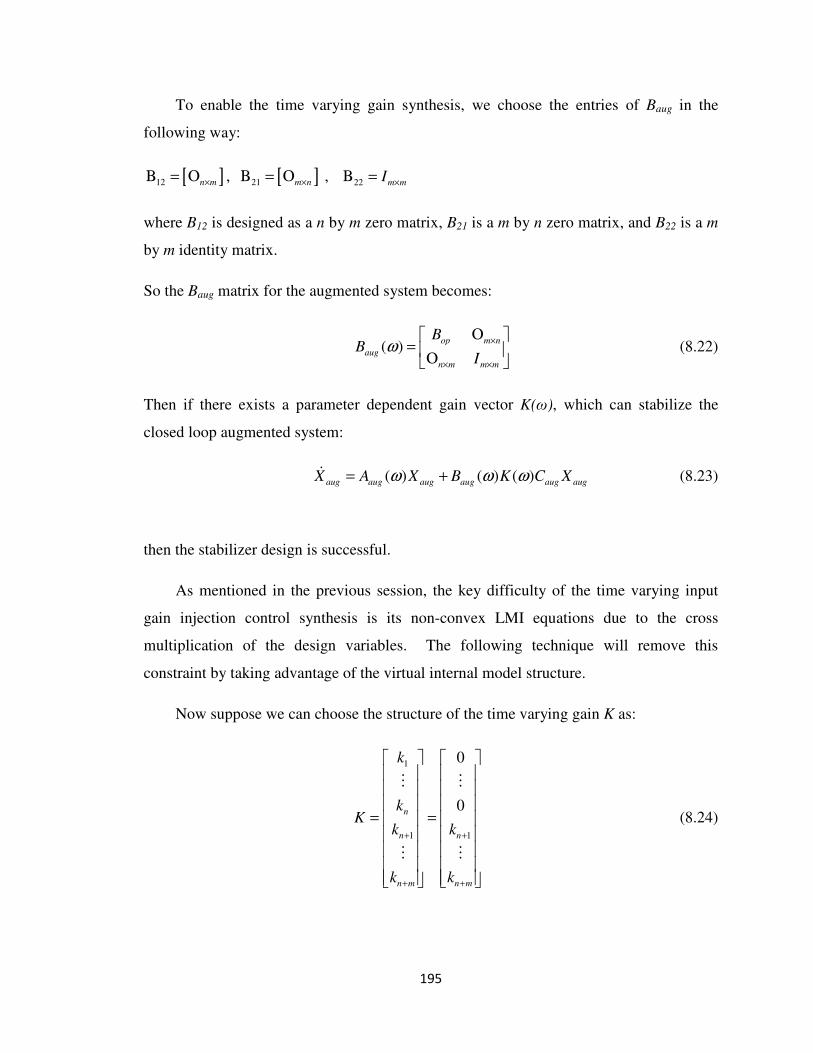
195

To enable the time varying gain synthesis, we choose the entries of Baug in the

following way:

[ ]12 n m×Β = Ο , [ ]21 m n×Β = Ο , 22 m mI ×Β =

where B12 is designed as a n by m zero matrix, B21 is a m by n zero matrix, and B22 is a m

by m identity matrix.

So the Baug matrix for the augmented system becomes:

( )op m n

aug

n m m m

BB

Iω ×

× ×

Ο = Ο

(8.22)

Then if there exists a parameter dependent gain vector K(ω), which can stabilize the

closed loop augmented system:

( ) ( ) ( )aug aug aug aug aug augX A X B K C Xω ω ω= +� (8.23)

then the stabilizer design is successful.

As mentioned in the previous session, the key difficulty of the time varying input

gain injection control synthesis is its non-convex LMI equations due to the cross

multiplication of the design variables. The following technique will remove this

constraint by taking advantage of the virtual internal model structure.

Now suppose we can choose the structure of the time varying gain K as:

1

1 1

0

0n

n n

n m n m

k

kK

k k

k k

+ +

+ +

= =

� �

� �

(8.24)

196

which means the first n elements of the gain K are forced to be zero. Here n is the

dimension or order of the plant dynamics, and m is the order of the internal model. In

general, the internal model order should be much higher than that of the plant order.

And define ( ) ( )

( ) ( )

1

...

...

...

1

I n m n m

n m n m

B I + × +

+ × +

= =

which is a (n+m) by (n+m) identity matrix.

It can be verified that

( ) ( ) ( )aug IB K B Kω ω ω= (8.25)

Then if there exists a time varying gain vector K(ω), which can stabilize the following

closed loop augmented system:

( ) ( ) ( ) ( )aug aug aug aug aug aug aug aug augX A X BK C X A X K C Xω ω ω ω= + = +� (8.26)

equally means that the designed control gain K(ω) can stabilize the original closed loop

system (8.23).

Therefore, we translate the time varying gain synthesis for system (8.23) to the time

varying injection gain design for system (8.26).

Then the above closed loop Lyapunov based LMI equation (8.17) can be written as:

1

( )( ) 0

sT T

aug aug aug aug i

i i

YYA YKC A Y KC Y

ωω

ω=

∂+ + + + <

∂∑ � (8.27)

==> 1

0s

T T T

aug aug aug aug i

i i

YYA YKC A Y C K Y ω

ω=

∂+ + + + <

∂∑ � (8.28)

==> 1

( )( ) 0

sT T T

aug aug aug aug i

i i

YYA YKC A Y C YK

ωω

ω=

∂+ + + + <

∂∑ � (8.29)

197

Suppose L=YK

==> 1

( )0

sT T T

aug aug aug aug i

i i

YYA LC A Y C L

ωω

ω=

∂+ + + + <

∂∑ � (8.30)

Note that there exists no design variable ( Y and L ) multiplication crossing terms in Eq

(8.30), thus the linear matrix inequality (8.30) above is convex. Using the interior point

optimization method, the variable Y and L can be obtained. Then the control vector K(ω)

can be derived as:

1( ) ( ) ( )K Y Lω ω ω−=

Remark: As shown in the derivation above, by selecting the specific Baug matrix and K

vector, the non-convex optimization problem can be transformed into a convex

optimization problem. The problem left is how to formulate and constrain the

optimization such that the first n elements of the designed K vector from Eq (8.31) below

are zero.

8.3.4 LMI Formulation To Synthesize Parameter Dependent Input Injection Gain

Vector K(ω)

The proposed approach is to design a time varying gain vector whose first n

elements are zero. As K is essentially an LMI inequality variable and obtained from the

multiplication of two LMI variables (Eq 8.31),

1

1

1

( ) ( ) ( )n

n

n m

k

kK Y L

k

k

ω ω ω−

+

+

= =

�

�

(8.31)

there is no guarantee that the K obtained from the LMI optimization would have the

feature required. In fact, currently there is no method to directly synthesize a K whose

198

first n elements are zero. Therefore, in the following, we will propose an indirect

approach based on two consecutive steps as listed in the following:

(1). The first step is to embed n uncertainty terms ∆1 up to ∆n in the first n elements

of the control gain vector K (Eq 8.31), such that a small perturbation on the time varying

injection gains will still stabilize the closed loop system.

(2). The second step is to constrain the maximum value of the first n elements of the

K vector, such that the maximum absolute value of k1 up to kn will not exceed max (|∆1|)

up to max (|∆n|). Thus even if k1 to kn are non-zero from the control synthesis but are

enforced to be zero in the real time implementation, the system will still be stable.

In the following further details about the two steps synthesis approach will be presented.

Step 1: Embedding uncertainty term in the control gain matrix:

Consider the augmented linear parameter varying system (8.21), assuming the control

input is

[ ( ) ] [ ( ) ] ( )aug K K aug aug

u K y K C Xω ω ω= + ∆ = + ∆ (8.32)

where

1

0

0

n

K

∆ ∆

∆ =

�

�

Note the uncertainty terms are only embedded in the first n rows.

Then the closed loop system (8.26) becomes:

199

1

1

[ ( ) ( ) ( )]0

0

[ ( ) ( ) ( ) ( )]0

0

n

aug aug aug aug

n

aug aug aug aug

X A K C X

A K C C X

ω ω ω

ω ω ω ω

∆ ∆

= + +

∆ ∆

= + +

�

�

�

�

�

(8.33)

Theorem 8.1: If the following linear matrix inequality holds:

1 1

1

( )( ) 0

0 0

0 0

T

sn nT T T

aug aug aug aug aug aug i

i i

YYA YKC Y C A Y KC Y C Y

ωω

ω=

∆ ∆ ∆ ∆ ∂

+ + + + + + < ∂

∑

� �

�

� �

(8.34)

for the uncertainty value spanning the whole range of [ ∆1min, ∆1max ] , [ ∆2min, ∆2max ] …

and [ ∆nmin, ∆nmax ], then the closed loop system Eq (8.26) will be quadratically stable

even with the perturbation K

∆ in the input injection control gain K.

Proof: Omitted. The proof is similar to the above LMI Lyapunov matrix formulation in

Eq (8.27). ■

However, in the optimization of the LMI Eq (8.34), we need to consider all the

uncertainties within the uncertainty range. This may involve intensive computation.

Fortunately, it is only necessary to consider the minimum and maximum value of the

uncertainty interval. This argument can be formally described as the following:

200

Theorem 8.2. Suppose

1

( )( ) ( )

sT T T T

K aug aug K aug aug aug aug K i

i i

Yf YA YKC Y C A Y KC Y C Y

ωω

ω=

∂∆ = + + ∆ + + + ∆ +

∂∑ �

If { }max minmax ( ), ( ) 0K Kf f∆ ∆ < , then ( ) 0K

f ∆ < for any min, max[ ]K K K

∆ ∈ ∆ ∆ .

Proof: The proof is straightforward due to the affine property of the uncertainty vector

K∆ . ■

Therefore it is only necessary to consider the maximum and minimum value of the

uncertainty boundary in the controller synthesis optimization, and all the control gain

perturbation within the uncertainties range can stabilize the closed loop system (8.26).

Step 2: Constraining the size of the first n elements in the parameter dependent input

injection control gain K(ω).

Now step 1 ensures that the system can be stabilized even though the parameter

dependent control gain K is perturbed by ∆K. Then if the maximum absolute value of k1

up to kn designed in LMI optimization are non-zero but does not exceed max (|∆1|) up to

max (|∆n|), the system will still be stable even if k1 to kn are set to be zero in the real time

control. Two methods (Theorem 8.3a and 8.3b) are proposed to realize the gain

constraint. They can constrain the norm individually, and either one could be used in the

controller synthesis ( The synthesis results shown in this thesis is based on 8.3a ). We will

present the following two theorems for constraining the norm of k1, and similarly k2 to kn

could be constrained in the same fashion.

Theorem 8.3 (a): For each discrete step i in the LMI optimization,, the Lyapunov

matrix Y and the variable vector L should satisfy all the following linear matrix

inequalities:

1 1

1

0T

G

G Y

α λ >

, 1Y Iα> , 0

T

LI L

L I

λ −<

− , (8.35)

where [ ]1 1 0 ... 0 0G = , then k1 is smaller than Lλ λ . ■

201

Proof: As 1

1 1k G Y L−= , we can first constrain the norm of 1

1G Y−

and L separately, then

the two norm of k1 will be constrained as well.

From 0T

LI L

L I

λ −<

− , by shur complement:

==> 0T

LL Lλ− + <

==>T

LL L λ<

==>2 LL λ<

To prove 1

1 2G Y λ− < , note that : 1Y Iα>

==>1

1

1Y I

α− <

==>1 1 1

1

1Y Y Y

α− − −<

==>1 1 1

1 1 1 1

1

1T TG Y Y G G Y G

α− − −<

Then if:

1

1 1

1

10

TG Y G λ

α− − <

==> 1 1

1 1 0T

G Y Y G λ− − − <

==> 1

1 2G Y λ− <

Therefore, according to Cauchy-Schwarz inequality, having the above LMI constraints

will ensure:

1 1

1 1 12 22 2 Lk G Y L G Y L λ λ− −= ≤ < . ■

202

Theorem 8.3 (b): For each discrete step i in the LMI optimization,, the Lyapunov

matrix Y and the variable vector L should satisfy all the following linear matrix

inequalities:

1 1

1

0T

G

G Y

λ >

, 2 0

TI L

L Y

λ −<

− , (8.36)

where [ ]1 1 0 ... 0 0G = , then k1 is smaller than 1 2λ λ . ■

Proof: From 2 0T

I L

L Y

λ −<

− , by shur complement:

==>1

2 0T

L Y Lλ −− + <

==>1/ 2

22Y L λ− <

In addition, from 1 1

1

0T

G

G Y

λ >

==>1

1 1 1 0T

G Y Gλ −− >

==>1

1 1 1

TG Y G λ− <

==>1/ 2

1 12G Y λ− <

Therefore, according to Cauchy-Schwarz inequality, having the above LMI constraints

will ensure:

1 1/ 2 1/ 2 1/ 2 1/ 2

1 1 1 1 1 22 2 2 2 2k G Y L G Y Y L G Y Y L λ λ− − − − −= = ≤ < . ■

8.3.5 Robust Input Gain Injection Controller Design

In this section, the robust control gain design considering the system model

uncertainty will be presented. Both the unstructured and structured uncertainty could be

embedded into the stabilizer synthesis. We will first discuss embedding the unstructured

203

uncertainty ( unmodeled dynamics ) into the parameter dependent input gain injection

synthesis.

As shown in Figure 8.3, the plant model uncertainty is considered at the output side.

( )clp aug clp

aug clp

x A x u

y C x

ω= +

=

�unstruct

∆( )e t ( )d t

( )K

K ω + ∆

...

Figure 8.3. Control loop with unstructured plant dynamics uncertainty

Now according to the small gain theorem, if 1/unstruct γ∞

∆ ≤ , then the induced L2

norm between e and d in Figure 8.3 should satisfy: 2 2

e d γ< for robust stability.

So the key problem is to formulate the appropriate conditions to constrain the

induced L2 norm and also enable the closed loop controller design based on a convex

LMI.

The closed loop system shown in Figure 8.3 can be represented as:

0( ) ( )

T T

aug aug K aug Kclp clp

aug

A KC C Kx x

Ce t d t

+ + ∆ + ∆ =

� (8.37)

In the following theorem and its proof, for presentation convenience, Aaug and Caug are

denoted as A and C respectively.

Theorem 8.4: If the following linear matrix inequality holds,

204

1

( )( ) ( )

0( ) 0

0

sT T T T T

K K i K

i i

T

K

YYA YKC Y C A Y KC Y C Y Y K C

K Y I

C I

ωω

ω

γ

γ

=

∂ + + ∆ + + + ∆ + + ∆ ∂

< + ∆ −

−

∑ �

(8.38)

then

(1). The nominal closed loop system is exponentially stable.

(2). The induced L2 norm between e and d is smaller than γ, thus the system is robustly

stable. ■

Proof: (1). See the appendix in this chapter.

In addition to the unstructured uncertainty, the plant structured parameter

uncertainty can be considered as well in the controller synthesis. If the boundary of the

parametric uncertainty S

∆ can be obtained in the experiment, then embedding the

structured uncertainty in the control design can alleviate the design conservativeness

comparing with using the unstructured uncertainty alone. The linear structured

uncertainty can be formulated as a LMI shown below. The proof is straightforward thus

is omitted.

1

( ) ( )

( )( )( )

0

( ) 0

0

T

S K S

TsKT T T

K i

i i

T

K

Y A YKC Y C A Y

Y K CYKC Y C Y

K Y I

C I

ωω

ω

γ

γ

=

+ ∆ + + ∆ + + ∆

+ ∆∂ + + ∆ + <∂ + ∆ −

−

∑ � (8.39)

8.3.6 Additional Control Gain Constraints

Two additional constraints can be added as well to improve the controller

performance and avoid saturation. First, the magnitude of the control gain ( )K ω should

be restricted in the controller synthesis optimization to avoid control saturation. Second,

205

constraints could be set for the Lyapunov matrix Y(ω) in Eq (8.38) to ensure fast

convergence rate.

Constraining the size of the input injection control gain K(ω).

Theorem 8.5: For each discrete step i, the Lyapunov matrix Y should satisfy the

following linear matrix inequality together with the conditions in Theorem 8.3:

0Y

Y I

I Iλ

>

, (8.40)

Then the 2 norm in the input gain vector K is smaller than Y Lλ λ . ■

Proof: See appendix in this chapter. ■

Controlling the Stabilizer Convergence Rate:

For each discrete step i, the Lyapunov matrix Y should satisfy:

1 2I Y Iα α< < (8.41)

1

( )( )

sT T

aug aug aug aug i

i i

YYA YKC A Y KC Y cI

ωω

ω=

∂+ + + + < −

∂∑ �

Then the state transition of the nominal closed loop system (8.26) will satisfy:

2 22

1 2

( ) (0) expclp clp

cX t X t

α

α α

< −

The proof is omitted as the conditions above are commonly used for exponential

convergence.

8.4 Experimental Investigation and Results

In the experimental study, the engine start torque oscillation rejection will be

simulated in the hydraulic dynamometer system. As the engine pumping torque pulse is

a frequency varying signal, whose frequency is proportional to the engine speed ( see

206

details in Chapter 7 ), the loading torque with similar shape should be generated by the

hydraulic actuator to compensate the torque vibration from the engine. As the pressure

difference in the dynamometer hydraulic system is closely related to the loading torque,

for experiment convenience, we define the control target as the pressure tracking of a

chirp signal. The frequency of the chirp signal will change and go up quickly to simulate

the situation in the engine start. So the key is to design a time varying internal model

controller and its stabilizer to track this signal with varying frequency.

The hydrostatic dynamometer system consists of a hydraulic control system, a 4

cylinder diesel engine and a number of sensing devices. A detailed photograph of the

main hardware in the hydrostatic dynamometer system is shown in Figure 8.4(a). The

hydraulic system of the hydrostatic dynamometer is shown in Figure 8.4(b). The main

hydraulic components are: a boost pump and an engine load (EL) pump/motor (both are

variable displacement piston pumps), a load-sensing control (LSC) valve (proportional

valve), and a high-speed control (HSC) valve (two-stage pilot valve, shown in the bottom

right corner of Figure 8.4(b)).

In the load-sensing feedback loop, the LSC valve regulates the inlet (operating)

pressure of the EL pump/motor Pin in Figure 8.4(b) to hold a constant value. In the

engine loading/motoring loop, the HSC valve, as the primary actuator, controls the outlet

pressure of the EL pump/motor Pout. The displacement adjustment mechanism, as the

secondary actuator, controls the displacement of the EL pump/ motor. Since the

dynamometer torque is a function of the displacement and pressure drop, and also we can

keep the inlet pressure Pin nearly constant, generating a frequency varying torque output

can be translated into the outlet pressure regulation to generate frequency varying outlet

pressure pulses. And this is exactly the target in the following experiments.

207

Figure 8.4 (a). Picture of hydrostatic dynamometer system

Figure 8.4 (b). Schematic diagram of the hydrostatic dynamometer

8.4.1 System Dynamics Modeling and Controller Design

The hydraulic system dynamics model includes a first order pilot operated valve

model and a first order pressure dynamics. The second order model can be written as:

2( )

L

L d u

L L b u

V PP W H C A L

τ

β ρ

= − +

= −

�

� (8.42)

208

where L is the valve spool displacement, τ is the inverse of the valve time constant, bL is

the valve voltage/orifice coefficient, β is the bulk modulus of the hydraulic oil, V is the

chamber volume, WL is the rotational speed of the engine load (EL) pump/motor, H is the

EL pump/motor displacement, ρ is the hydraulic oil density, Au(L) is the orifice function.

The first order valve dynamics is a simplification of the pilot operated proportional

control valve. The plant model is a nonlinear because of the multiplication of the state P

and L. However, if P could be treated as a parameter measured on-line, then the system

could be regarded as a quasi linear parameter varying (LPV) system.

The reference signal to be tracked is a chirp signal with a varying frequency ω(t).

This kind of signal can be modeled as an exo-system [5]:

0 ( )( )

( ) 0

tS t

t

ω

ω

= −

(8.43)

with the reference signal ω(t) as the time varying parameter.

Both the exo-system model and the plant dynamics need to be transformed into the

observer canonical form to enable the time varying internal model design. The

transformed plant model can be written as:

1 1 1 2

2 0 1 0

1

o o o

o L o

o

x a x x

x W H a x b uV

y x

βτ

= − +

= − +

=

�

� (8.44)

where

2 2

0/b RHS V P Pβ τ τ= × +� , 1a τ= , 0 0a = , (8.45)

y is the output pressure.

And the exo-system in the observer canonical form is

1

0

( ) 1( )

( ) 0O

tS t

t

α

α

− = −

(8.46)

209

where

1

( )( )

( )

tt

t

ωα

ω= −�

and

22

0 2

( ) ( ) ( )( ) ( )

( )

t t tt t

t

ω ω ωα ω

ω

−= +

�� (8.47)

In addition, the L

W H in Eq (8.44) is assumed to be constant and known, so a feed-

forward input 0

d Lu W H

b V

βτ= − is used to compensate the constant term. Then the control

input u in Eq (8.44) becomes u=ud+ust, with ust denoting the control input from the LPV

stabilizer.

The time varying internal model can therefore be designed and the augmented

system ( the internal model + plant dynamics ) can be written as:

( ) ( ) ( ) ( )

( ) ( )

aug aug aug aug st

aug aug aug

X t A t X t B t u

Y t C X t

= +

=

�

(8.48)

where

1

0 0 1 0 2

1 2

( ) 1 0 0

( ) 0 ( ) ( ) ( ) ( )( )

0 0 0 1

0 0 ( ) ( )

aug

a t

a t b t t b t tA t

t t

γ γ

ϕ ϕ

− − =

(8.49)

2

1 0 0 0 0 0 0 0 1( / ) /a b q q p b q aϕ = − − − − −� � and

2 1 0 0/a b qϕ = − − (8.50)

2

1 0 0 0 0/ /q q p qγ = − +� ,

2 01/ qγ = (8.51)

0 0 1 1/( )q b aα= − , 0 0 0 1 1 0 0( ) /( ) /p a a b bα α= − − + � (8.52)

To enable robust stabilizer design, the Baug matrix in Eq(8.48) is designed as

0

0 0 0 0

0 ( ) 0 0( )

0 0 1 0

0 0 0 1

aug

b tB t

=

(8.53)

210

Note that b0 is the only non-zero and non-unit term. In this case, instead of enforcing

both the first two gains k1 and k2 in the control gain K to be zero, it is only necessary to

constrain the k1 to be zero. That is:

1

2 2

3 3

4 4

0

aug

k

k kK

k k

k k

= =

(8.54)

And K

∆ for the control gain synthesis is

[ ]1 0 0 0T

K∆ = ∆ (8.55)

To see this point, define

4 4

1 0 0 0

0 1 0 0

0 0 1 0

0 0 0 1

IB I ×

= =

(8.56)

It can be verified that

22

0

33

44

00

( )I aug

kk

bB B tk

kk

k

=

(8.57)

From which we can see that if Kaug in Eq(8.54) can stabilize

( )aug aug aug I aug aug augX A X B K C Xω= +� (8.58)

equally means that the designed control gain 23 4

0

0T

kk k

b

can stabilize the closed

loop system of (8.48)

211

( ) ( )aug aug aug aug aug augX A t X B t KC X= +� (8.59)

In other words, after obtaining [ ]2 3 40T

k k k from the optimization based control

synthesis for the closed loop system (8.59), the real time time-varying control gain could

be set to be 23 4

0

0T

kk k

b

.

So the target for the LPV synthesis is to design the time varying input injection gain

whose first element is zero to stabilize the augmented system (8.48) in a robust fashion.

8.4.2 Experimental Results and Discussion

The system dynamics (Eq. 8.42) has been identified for the second order hydraulic

system. It’s hard to use a second order model to precisely describe the pressure together

with the valve dynamics covering a wide frequency range. In particular, to have the

model simulation match the experimental data, the τ in Eq (8.42 ) needs to be small for

high frequency input and large for low frequency input. While using a higher order model

will give better model matching result, it will induce control design complexity. So in

the controller synthesis, we use a small τ (τ =12 ) , which will make the dynamic model

imprecise for low frequency region. However, the uncertainty in the second order model

can also be a test for the robustness of the control method.

The time varying internal model is first designed, and the time varying stabilizer

gains are synthesized as shown in Figure 8.5 based on the proposed design method in Sec.

8.3. It can be seen that the gain k1 is constrained into a fairly small value comparing with

k2 and k4. K∆ in Eq (8.55) for Kaug (Eq. 8.54) is chosen to be in the interval from [-200 0

0 0]T to [200 0 0 0]

T, which can bound the gain k1 throughout the parameter range shown

in Figure 8.5. Therefore setting k1 to be zero in the real time implementation will not

destabilize the system.

212

10 12 14 16 18 20 22 24 26

-100

-50

0

gain

k1

10 12 14 16 18 20 22 24 26-4

-2

0x 10

4

gain

k2

10 12 14 16 18 20 22 24 26

-40

-20

0

gain

k3

10 12 14 16 18 20 22 24 260

2

4x 10

4

gain

k4

Frequency w (Hz)

Figure 8.5 Time varying input injection gains

The designed time varying internal model together with the stabilizer is then

implemented in the hydro-dynamometer system. Three groups of experiments are shown

from Figure 8.6 to Figure 8.8.

In the first group, the reference signal frequency variation rate is 4.8 Hz/sec, and the

frequency is changing from 10 Hz to 25Hz in nearly three seconds as shown in Figure

8.6(a). The tracking error converges fast within the two cycles as shown in Figure 8.6(b).

The control input shown in Figure 8.6(c) presents a frequency varying control command

with magnitude variation even in the steady states. As mentioned earlier, it’s hard to use

the second order model to describe the system dynamics covering a wide frequency range,

and the model uncertainties are inevitable. Nevertheless, the successful pressure tracking

and stabilization results shown in Figure 8.6 indicates the robustness of the time varying

stabilizer design. To further study the stabilizer robustness, we add 20% perturbation to

213

the parameter b0 in the internal model (Eq 8.49), and the system can still be stabilized and

exhibit similar tracking results as shown in Figure 8.6.

In the second test, the b0 in Eq (8.45) is further perturbed by 4 times of its original

value and therefore the internal model designed (8.49) has larger perturbation comparing

with the first group of experiment. We first let the system track a reference with slower

frequency variation of 0.79 Hz/sec. Figure 8.7 shows the pressure tracking results of a

chirp signal with varying frequency between 10 Hz to 29.75 Hz in 25 second. The signal

frequency variation can be observed from Figure 8.7(a), which also shows that the

controlled pressure converges to the reference pressure slowly at the initial stage. The

slow convergence is mainly due to the internal model parameter perturbation. Figure 8.7

(b) and (c) present the zoom-in view of tracking result for one second at two different

frequency ranges, which clearly indicates the frequency difference. The control

command shown in Figure 8.7(d) again exhibits the magnitude varying feature of the

input.

In the third experiment, the b0 in Eq (8.45) is still perturbed the same amount as the

second test (four times of its original value), but the tracking reference signal is the same

as the first group of experiment, which has a much faster frequency variation rate of

4.8Hz/sec. As shown in Figure 8.8(a), the controller can no longer maintain good

tracking results as it does in the slow frequency varying case ( Figure 8.7). This is

because the faster frequency variation rate (4.8 Hz/sec vs 0.79Hz/sec) will affect 1( )tα

and 0 ( )tα in Eq (8.47) and subsequently q0 and γ2 in Eq (8.52) and Eq (8.51), which will

then amplify the effect of the perturbation of b0(t) in the internal model Eq (8.49).

Therefore, we can conclude that the stabilizer is robust since the model uncertainty

and small perturbation will not cause instability. For large parameter perturbation, the

system can keep reasonable tracking for smooth frequency varying, but the error starts

diverging in the case of aggressive frequency variation.

214

105 105.5 106 106.5 107

10

15

20

25

time (s)

pre

ssure

(bar)

Reference vs pressure

Real pressure

Reference

Figure 8.6 (a). Pressure tracking with 4.8Hz/sec frequency variation rate

105 105.5 106 106.5 107-5

0

5

time (s)

Err

or

(bar)

Tracking Error

Error

Reference

Figure 8.6 (b). Pressure tracking error vs shifted reference

215

105 105.5 106 106.5 107

-0.8

-0.6

-0.4

-0.2

0

0.2

0.4

0.6

time (s)

contr

ol in

put

(volt)

Control Input

Control Voltage Input

Figure 8.6 (c). Valve control voltage input

150 150.5 151 151.5 152 152.5 153 153.5 154 154.5 155

12

14

16

18

20

22

24

time (s)

pre

ssure

(bar)


Real pressure

Reference

Figure 8.7 (a). Zoom-in view of pressure tracking at the start with 0.79Hz/sec frequency variation

161 161.2 161.4 161.6 161.8 162

12

14

16

18

20

22

24

time (s)

pre

ssure

(bar)


Real pressure

Reference

173 173.2 173.4 173.6 173.8 174

12

14

16

18

20

22

24

time (s)

pre

ssure

(bar)


Real pressure

Reference

Figure 8.7 (b). zoom-in view at 161 sec Figure 8.7 (c). zoom-in view at 173 sec

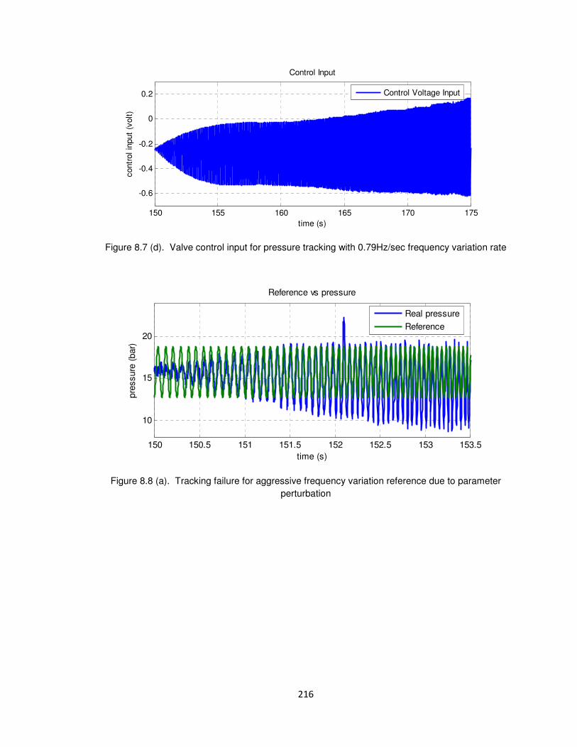
216

150 155 160 165 170 175

-0.6

-0.4

-0.2

0

0.2

time (s)

contr

ol in

put

(volt)

Control Input


Figure 8.7 (d). Valve control input for pressure tracking with 0.79Hz/sec frequency variation rate

150 150.5 151 151.5 152 152.5 153 153.5

10

15

20

time (s)

pre

ssure

(bar)


Real pressure

Reference

Figure 8.8 (a). Tracking failure for aggressive frequency variation reference due to parameter

perturbation

217

150 150.5 151 151.5 152 152.5 153 153.5-1.5

-1

-0.5

0

0.5

1

time (s)

contr

ol in

put

(volt)

Control Input


Figure 8.8 (b). Valve control input

TABLE 8.1. SYSTEM PARAMETERS

TABLE 1. System parameters in the dynamic models

Symbol Description Quantity

β

V

RHS

H

effective bulk modulus

chamber volume

RHS=CdAHS(ρ)1/2

(m3/sec/Pa

1/2)

EL pump displacement

1.3e9 (Pa)

2e-4 (m3)

1.05e-5

107 (cc/rev)

8.5 Conclusion

As a conclusion, the problem defined in this chapter is the tracking/rejection control

of a periodic signal/disturbance for a linear parameter varying (LPV) plant dynamics

based on the internal model principle. A low order and computationally efficient robust

stabilizer design for the LPV internal model control is still an open problem and not

available previously. A promising approach is proposed to solve this problem, which is

the key contribution in this chapter. The proposed method is enabled by the unique

dynamics characteristic of the internal model system, and translates a non-convex

controller synthesis into a convex optimization based control design. To this end,

experiments are conducted to verify the proposed control methodology using the

hydrostatic dynamometer system, and the synthesized controller is shown to be efficient,

low order, and robust.

218

8.6 Appendix in Chapter 8:

Proof for Theorem 8.4

Proof: (1). By Shur complement, the LMI (8.40) above can be converted into the

following Riccati equation:

1

( )( )

1 1( )( ) 0

sT T T T

K K i

i i

T T

K K


C C Y K K Y

ωω

ω

γ γ

=

∂+ + ∆ + + + ∆ +

∂

+ + + ∆ + ∆ <

∑ �

As 1 1

( )( )T T

K KC C Y K K Y

γ γ+ + ∆ + ∆ is positive semi-definite, then

1

( )( ) 0

sT T T T

K K i

i i


ωω

ω=

∂+ + ∆ + + + ∆ + <

∂∑ �

So the nominal closed loop system is quadratically stable, which equally means

exponential stability in the linear time varying case. ■

Proof: (2):

Define the Lyapunov function for closed loop system (8.39) as ( ) T

clp clp clpV x x Yx=

( ) ( ) ( )T

clp K clp Kx A KC C x K d t= + + ∆ + + ∆�

The time derivative of the Lyapunov function V is

1

( )( ) ( )

( ) ( ) ( )( )

sT T T T T

clp clp K K i clp

i i

T T T T T

clp K K clp

d YV x x YA YKC Y C A Y KC Y C Y x

dt

x Y K d t d t K Yx

ωω

ω=

∂= + + ∆ + + + ∆ +

∂

+ + ∆ + + ∆

∑ �

As

219

1

( )( )

1 1( )( )

sT T T T

K K i

i i

T T

K K


C C Y K K Y

ωω

ω

γ γ

=

∂+ + ∆ + + + ∆ +

∂

< − − + ∆ + ∆

∑ �

==>

1 1( ) ( )( )

( ) ( ) ( )( )

T T T

clp clp K K clp

T T T T T

clp K K clp

dV x x C C Y K K Y x

dt

x Y K d t d t K Yx

γ γ

< − − + ∆ + ∆

+ + ∆ + + ∆

==>

1 1( ) ( )( ) ( ) ( ) ( ) ( )

( ) ( ) ( )( )

T T T T T

clp clp K K clp

T T T T T

clp K K clp

dV x x C C Y K K Y x d t d t d t d t

dt

x Y K d t d t K Yx

γ γγ γ

< − − + ∆ + ∆ − +

+ + ∆ + + ∆

==>

( ) ( ) ( ) ( ) ( )( )

( ) 1( )( )

1( ) ( )

T T T T T T

clp K K clp

clp T T

clp K K clp

T T T

clp clp

d t d t x Y K d t d t K Yxd

V xdt x Y K K Yx

d t d t x C Cx

γ

γ

γγ

− + ∆ − + ∆

< − + + ∆ + ∆

+ −

==>

1 1( ) ( ) ( ) ( ) ( )

1( ) ( )

T

T T

clp K clp K clp

T T T

clp clp

dV x d t K Yx d t K Yx

dt

d t d t x C Cx

γ γγ γ

γγ

< − − + ∆ − + ∆

+ −

Integrate both sides:

==>

2

2 2

2 2

2

1 10 ( ) ( ) ( ) ( )

T

K clpV d t K Yx d t e tγ γ

γγ< < − − + ∆ + −

Therefore 2

2

( )

( )

e t

d tγ<

Therefore the system will be robustly stable if the L2 norm of the unstructured uncertainty

is less than 1/γ. ■

220

Proof for Theorem 8.5

Proof: From Theorem 8.3 (a), we have already proved that 2 LL λ< .

In addition, as 0Y

Y I

I Iλ

>

, by shur complement,

==> 1

YY Iλ− <

==> 1T T

Yx Y x x xλ− < , where x is any vector belonging to R

n.

==>2 21

2 22 Yi

Y x xλ− <

==> 1

2 Yi

Y λ− <

where 1

2iY

− is the induced matrix two norm.

Therefore, according to the induced matrix norm consistency condition,

1 1

2 22 2 Y Li

K Y L Y L λ λ− −= < < . ■

221


[1] B.A. Francis. The internal model principle of control theory. SIAM Journal of

Control, vol. 15 (3), pp. 486-505, 1977.

[2] B.A. Fancis, and W.M. Wonham. The internal model principle of control theory.


[3] K.S. Tsakalis, P.A. Ioanou, Linear Time-Varying Systems: Control and Adaptation, in:

Advances in Industrial Control, Prentice Hall, Englewood Cliffs, NJ, 1993

[4] A. Isidori, C.I. Byrnes, Output regulation of nonlinear systems, IEEE Transactions on

Automatic Control 35 (2) (1990), 131-140

[5] Z. Sun, Z. Zhang, and T.-C. Tsao. Trajectory tracking and disturbance rejection of


Letters, vol. 58 (6): 452-460, 2009.

[6] A.Ichikawa, H.Katayama, Output regulation of time-varying systems, IEEE


[7] Z. Zhang, A. Serrani, The linear periodic output regulation problem, Systems &


[8] S. Hara, Y. Yamamoto, T. Omata, and M. Nakano. Repetitive control systems: a new

type servo system for periodic exogenous signals. IEEE Transactions on Automatic

Control, 33(7):659-668, 1988.

[9] M. Tomizuka, T.-C. Tsao, and K.-K. Chew. Analysis and synthesis of discrete-time



[10] T.-C. Tsao and M. Tomizuka. Robust adaptive and repetitive digital tracking control

and application to hydraulic servo for noncircular machining. ASME Transactions on

Journal of Dynamic Systems, Measurement and Control, 116 (1):24-32, 1994.

[11] Shamma, J. S., & Athans, M. (1990). Analysis of nonlinear gain scheduled control

systems. IEEE Transactions on Automatic Control, AC-35(8), 898-907.

222

[12] Rugh, W. J. and Jeff S. Shamma (2000). Research on gain-scheduling. Automatica,

36, 1401-1425.

[13] Packard, A. (1994). Gain-scheduling via linear fractional transformations. Systems

and Control Letters, 22, 79-92.

[14] Reichert, R. (1992). Dynamic scheduling of modern-robust-control autopilot designs

for missiles. IEEE Control Systems Magazine, 12(5), 35-42.

[15] Rugh, W. J. (1983). Linearization about constant operating points: An input-output

viewpoint. Proceedings of the IEEE conference on decision and control, San

Antonio, TX (pp. 1165-1169).

[16] Rugh, W. J. (1991). Analytical framework for gain-scheduling. IEEE Control

Systems Magazine, 11(1), 79-84.

[17] Shahruz, S. M., & Behtash, S. (1992). Design of controllers for linear parameter-

varying systems by the gain scheduling technique. Journal of Mathematical Analysis

and Applications, 168(1), 195-217.

[18] Shamma, J. S., & Athans, M. (1991). Guaranteed properties of gain scheduled

control of linear parameter-varying plants. Automatica, 27(3), 898-907.

[19] Shamma, J. S., & Cloutier, J. R. (1992). Trajectory scheduled missile autopilot

design. Proceedings of the first IEEE conference on control applications, Dayton,

OH, September.

[20] Shamma, J. S., & Xiong, D. (1999). Set-valued methods for linear parameter

varying systems. Automatica, 35(6), 1081-1089.

[21] Stilwell, D. J., & Rugh, W. J. (2000). Stability preserving interpolation methods for

the synthesis of gain scheduled controllers. Automatica, 36(5), 665-671.

[22] P. Apkarian and P. Gahinet, “A convex characterization of gainscheduled H_inf

controllers,” IEEE Trans. Automat. Contr., vol. 40, pp. 853–864 and p. 1681, May

1995.

223

[23] G. Becker, A. Packard, D. Philbrick, and G. Balas, “Control of parametrically-

dependent linear systems: A single quadratic Lyapunov approach,” in Proc. Amer.

Contr. Conf., San Fransisco, CA, 1993, pp. 2795–2799.

[24] P. Apkarian, P. Gahinet, and G. Becker, “Self-scheduled H_inf control of linear

parameter-varying systems: A design example,” Automatica, vol. 31, pp. 1251–

1261, Sept. 1995.

[25] F. Wu, X. Yang, A. Packard, and G. Becker, “Induced L2-norm control for LPV

system with bounded parameter variations rates,” in Proc. Amer. Contr. Conf.,

Seattle, WA, 1995, pp. 2379–2383.

[26] P. Gahinet, P. Apkarian, and M. Chilali, “Parameter-dependent Lyapunov functions

for real parametric uncertainty,” IEEE Trans. Automat. Contr., vol. 41, pp. 436–442,

1996.

[27] E. Feron, P. Apkarian, and P. Gahinet, “Analysis and synthesis of robust control

systems via parameter-dependent Lyapunov functions,” IEEE Trans. Automat.

Contr., vol. 41, pp. 1041–1046, July 1996.

[28] G. Becker, “Parameter-dependent control of an under-actuated mechanical system,”

in Proc. IEEE Conf. Decision Contr., 1995.

[29] P. Apkarian, “On the discretization of LMI-synthesized linear parameter varying

controllers,” Automatica, vol. 33, pp. 655–661, 1997.

[30] P. Gahinet and P. Apkarian, “A linear matrix inequality approach to H_inf control,”

Int. J. Robust and Nonlinear Contr., vol. 4, pp. 421–448, 1994.

[31] P. Gahinet, “Explicit controller formulas for LMI-based H1 synthesis,” in Proc.

Amer. Contr. Conf., 1994, pp. 2396–2400.

[32] G. Becker, “Additional results on parameter-dependent controllers for LPV systems,”

in IFAC World Congr., San Fransisco, CA, 1996.

[33] S. Boyd and L. El Ghaoui, “Method of centers for minimizing generalized

eigenvalues,” Linear Algebra Applicat., vol. 188, pp. 63–111, Apr. 1992.

224

[34] P. Apkarian and R. Adams, “Advanced gain-scheduling techniques for uncertain

systems,” in Proc. Amer. Contr. Conf., June 1997, pp 3331–3335.

[35] V.L.Syrmos, C.T. Abdallah, P. Dorato, and K. Grigoriadis, “Static Output

Feedback—A Survey,” in Automatica.,ol.33, No.2, pp125-137, 1997.

[36] A.I. Zecevic and D.D.Siljak, “Design of Robust Static Output Feedback for Large-

scale Systems,” in IEEE Trans. Automat. Contr., vol. 49, No.11, pp. 2040–2044,

Nov 2004.

[37] Zhang, Z., and Sun, Z., 2010. “A novel internal model based tracking control for a

class of linear time-varying systems”. ASME Journal of Dynamic Systems,

Measurement and Control, 132(1), pp. 011004–1–10.

[38] El Ghaoui, L. and P. Gahinet (1993). Rank minimization under LMI constraints: a

framework for output feedback problems. In Proc. European Control. Co&

Groningen, pp. 1176-1179.

[39] Grigoriadis, K. M. and R. E. Skelton (1993). Low-order control design for LMI

problems using alternating projection methods. In Proc. 31st Allerton Conf on

Communication, Control and Computing, Urbana-Champaign, IL. pp. 231-240.

[40] Grigoradis, K. M., & Skelton, R. E. (1996). Low-order control design for LMI

problems using alternating projection methods. Automatica, 32(8), 1117–1125.

[41] L.H.Lee, Identification and Robust Control of Linear Parameter Varying Systems,

Ph.d. dissertation, Department of Mechanical Engineering, University of California

at Berkeley (1997).

225

Chapter 9

Conclusion, Contributions Summary and Future Work

9.1 Conclusion

In conclusion, this thesis focuses on the design, dynamic analysis and control

methodologies, which can enable the smooth and efficient power transmission for

conventional, hybrid and future automotive propulsion systems. We formulate the

problem in three levels: the basic clutch level, the intermediate driveline level and the

entire propulsion system level. The critical research problems are revealed for each level,

and the resolving design and control solutions are proposed accordingly.

First, for the clutch level, to realize a precise and efficient clutch actuation, the

enabling approaches are presented in two categories: open loop and closed loop clutch

control. The open loop actuation considers the consistent initial condition and the clutch

fill process optimization. In the closed loop case, the solutions are further divided into

two groups: the feedback control with sensor measurement and the closed loop control

without sensor feedback. Second, for the driveline level, optimal driveline coordination

is formulated into a nonlinear optimization problem, which is solved using the Dynamic

Programming. Finally, for the propulsion system level, the power source start/stop

torque pulses rejection is treated as a disturbance rejection using the time varying internal

model framework. Two critical issues are addressed. One is the tracking control of the

periodic signal with magnitude variation, and the other is the low order and robust

stabilizer design for the time varying internal model controller. Both of them are the

fundamental issues for the internal model control framework, and the research outcome

can be potentially applied to other applications beyond the automotive field as well.

9.2 Contributions Summary

The contributions of this thesis span from the control applications to the

fundamental control theory. Application wise, this thesis formulates the smooth and

efficient power transmission design and control problem in three levels, and proposes

226

design, dynamics analysis and control methodologies to address the critical challenges in

each level respectively. For control theory, a robust and low order stabilizer synthesis

method is proposed to enable reference tracking/disturbance rejection based on linear

time varying internal model principle. This thesis addresses one of the most crucial

issues in the linear time varying internal model control synthesis, which enables

experimental investigation of the internal model controller in the LTV setting.

9.2.1 Contributions in power transmission applications:

(1). Formulate the consistent initial condition control into an optimal ball capsule

shape design using Dynamic Programming. Provide the mathematical derivation of the

unique asymmetric valve orifice, which is not available in the literature. Reveal that the

system dynamic instability is the key to realize fast response.

(2). Formulate the optimal clutch fill problem, and propose a novel customized

dynamic programming method. The method can successfully avoid the stiff hydraulic

dynamics which otherwise will cause intensive optimization computation for the control

design. It can also avoid the interpolation error and the unreachable discrete states

associated with the conventional DP. Experiments conducted to verify the control

scheme.

(3). This thesis is the first research summary systematically documenting the

analysis of the unique dynamics of the “wet” clutch actuation. It presents a systematic

approach for controlling the “wet” clutch with only pressure feedback. More specifically,

first, several unique phenomena of the “wet” clutch dynamics are revealed and are used

to guide the robust control (sliding mode + observer) design. This makes the proposed

control method more effective for this type of clutch system. Second, while directly

applying the sliding mode controller may cause chattering, two approaches to constrain

the feedback gain are applied and proved to be effective in the experiment. Finally, a

nonlinear observer is designed to estimate the clutch motion with only pressure

measurement.

(4). Propose a novel clutch control mechanism to realize closed loop control with no

electronic sensor measurement. The feedback is realized by a built-in hydra-mechanical

structure, and would ensure clutch fill preciseness and robustness comparing with pure

227

open loop control. Prototype was fabricated, dynamics model built, and experimental

tests exhibit reliable and precise results.

(5).The optimal mathematical descriptions for smooth driveline coordination and

slipping heat minimization formulated. Propose applying Dynamic Programming to

solve the optimal engagement for automated manual transmission, which involves non-

quadratic cost function and nonlinear dynamics. Comparing with existing suboptimal

solution with quadratic cost function approximations, the results obtained are closer to

the optimal solution.

(6). Apply the angle based repetitive control to fulfill the energy efficient vibration

rejection for hybrid vehicle. The engine torque disturbance characteristics analyzed, and

the corresponding controller synthesis provided.

9.2.2 Contributions in control theory:

(1). Based on the time varying internal model principle, formulate the tracking

control of a unique group of signals, the periodic signal with magnitude variation. Derive

its generating dynamics, and provide the asymptotic tracking control design.

(2). Solves a fundamental bottleneck problem in the linear time varying internal

model control theory by proposing a novel low order robust stabilizer design. Convert

the control synthesis conditions into a sequence of Linear Matrix Inequality (LMI)

constraints, which could be solved efficiently by optimization algorithms. The significant

impact is to enable the experimental realization of the linear time varying internal model

control. The research results could potentially enable a wide class of control design based

on linear time varying internal model principle, such as the repetitive control for linear

time varying system.

9.3 Future Work

The future work will be outlined based on the three levels. First, for the clutch level,

the designed ball capsule system (Chapter 2) is expected to be fabricated and tested in the

experiment. Both the optimal design results and the derived asymmetric valve orifice

equation should be verified from the experimental study. In addition, although the

228

optimal clutch fill (Chapter 3), the pressure based closed loop clutch actuation (Chapter 4)

and the hydra-mechanical feedback clutch mechanism design (Chapter 5) have been

evaluated with solid experimental data, the in-vehicle tests are expected to further

demonstrate their effectiveness and robustness in different working environments.

What’s more, further design optimization on the novel hydra-mechanical feedback based

clutch mechanism (Chapter 5) is expected. For example, the size of the system could be

smaller to make it compact for transmission assembly. Second, for the driveline level

design, the current Dynamic Programming based optimal coordination design (Chapter 6)

is relatively computational intensive, therefore the study on the more computational

efficient optimization method could be the research work in the next step. For the

propulsion system level design, research on the angle based repetitive control for linear

time varying plant using the proposed parameter dependent gain injection stabilizer

(Chapter 8) will be the study for the next step. This control synthesis further requires

extending the current continuous time LPV stabilizer design method to the discrete case,

and then implementing the high order time varying repetitive controller for the

experimental setup.

229

Bibliography1

• A.I. Zecevic and D.D.Siljak, “Design of Robust Static Output Feedback for Large-

scale Systems,” in IEEE Trans. Automat. Contr., vol. 49, No.11, pp. 2040–2044,

Nov 2004.

• A. Isidori, C.I. Byrnes, Output regulation of nonlinear systems, IEEE Transactions

on Automatic Control 35 (2) (1990), 131-140

• A. Bemporad, F. Borrelli, L. Glielmo, and F. Vasca, “Hybrid control of dry clutch

engagement,” in Proc. European Control Conf., Porto, Portugal, 2001.

• A. Szadkowski and R. B. Morford, “Clutch engagement simulation: Engagement

without throttle,” SAE Tech. Paper Series, no. 920766, 1992.

• A.Ichikawa, H.Katayama, Output regulation of time-varying systems, IEEE


• Bai, S., Moses, R.L, Schanz, Todd and Gorman, M.J. “Development of A New


• Bellman, R., 1957, Dynamic Programming, Princeton University Press, New Jersey.

• Bellman, R. and Dreyfus, S., 1962, Applied Dynamic Programming, Princeton


• Bertsekas, D., Dynamic Programming and Optimal Control, Athena Scientific, 1995.

• Baumann, J., Torkzadeh, D.D., Ramstein, A., Kienke, U., and Schelegl, Model-

based predictive anti-jerk control T. Control Engineering Practice, 14, 259–266

(2006).

• Balfour, G., Dupraz, P., Ramsbottom, M., and Scotson, Diesel fuel injection control

for optimum driveability SAE 2000-01-0265.

• B.A. Francis. The internal model principle of control theory. SIAM Journal of

Control, vol. 15 (3), pp. 486-505, 1977.

• B.A. Fancis, and W.M. Wonham. The internal model principle of control theory.


1 The numbered references in each chapter refer to the reference lists at the end of each chapter, and the

cumulative bibliography here summarizes all the cited work throughout the thesis.

230

• Crassidis, J.L. and Junkins, J.L. “Optimal Estimation of Dynamic Systems”.


Express LLC, 2004.

• Daekyun Kim, Huei Peng, Shushan Bai, and Joel M. Maguire. “Control of Integrated

Powertrain with Electronic Throttle and Automatic Transmission.” IEEE

Transactions on Control Systems Technology, Vol. 15, Issue 3, pp. 474 – 482, May

2007

• De Madrid, A.P. Dormido, S., and Morilla, F., “Reduction of the Dimensionality of

Dynamic Programming: A Case Study,” Pro. Of 1999 American Control

Conference, pp 2852-2856, June 1999

• D. Centea, H. Rahnejat, and M. T. Menday, “The influence of the interface

coefficient of friction upon the propensity to judder in automotive clutches,” Proc.

Inst. Mech. Eng., vol. 213, pt. D, pp. 245–268, 1999.

• DeLaSalle, S., Jansz, M., and Light, D. (1999), Design of a Feedback Control

System for Damping of Vehicle Shuffle. Proceedings of the EAEC Conference,

Barcelona, pp 278–284.

• E. Feron, P. Apkarian, and P. Gahinet, “Analysis and synthesis of robust control

systems via parameter-dependent Lyapunov functions,” IEEE Trans. Automat.

Contr., vol. 41, pp. 1041–1046, July 1996.

• El Ghaoui, L. and P. Gahinet (1993). Rank minimization under LMI constraints: a

framework for output feedback problems. In Proc. European Control. Co&

Groningen, pp. 1176-1179.

• E. M. A. Rabeih and D. A. Crolla, “Intelligent control of clutch judder and shunt

phenomena in vehicle drivelines,” Int. J. Veh. Des., vol. 17, no. 3, pp. 318–332,

1996

• F. Garofalo, L. Glielmo, L. Iannelli, and F. Vasca, “Smooth engagement for

automotive dry clutch” in Proc. 40th IEEE Conf. Decision and Control, Orlando, FL,

2001, pp. 529-534

231

• F. Amisano, G. Serra, and M. Velardocchia, “Engine control strategy to optimize a

shift transient during clutch engagement,” SAE Tech. Paper Series, no. 2001-01-

0877, pp. 115–120, 2001.

• F. Amisano, R. Flora, and M. Velardocchia, “A linear thermal model for an

automotive clutch,” SAE Tech. Paper Series, no. 2000-01-0834, 2000.

• F. Wu, X. Yang, A. Packard, and G. Becker, “Induced L2-norm control for LPV

system with bounded parameter variations rates,” in Proc. Amer. Contr. Conf.,

Seattle, WA, 1995, pp. 2379–2383.

• Gautschi, W., 1997. Numerical Analysis: An Introduction, Birkhauser Boston

• Gao, B., Chen, H., Sanada, K., Hu, Y., “Design of Clutch-Slip Controller for

Automatic Transmission Using Backstepping,” IEEE/ASME Transactions on

Mechatronics, in press, 2010.

• Gao, B., Chen, H., Sanada, “A Reduced Order Nonlinear Clutch Pressure Observer

for Automatic Transmission,” IEEE Transactions on Control Systems Technology,

Vol. 18, Issue.2, pp. 446-453, March., 2010.

• G. Becker, “Additional results on parameter-dependent controllers for LPV

systems,” in IFAC World Congr., San Fransisco, CA, 1996.

• G. Becker, “Parameter-dependent control of an under-actuated mechanical system,”

in Proc. IEEE Conf. Decision Contr., 1995.

• G. Becker, A. Packard, D. Philbrick, and G. Balas, “Control of parametrically-

dependent linear systems: A single quadratic Lyapunov approach,” in Proc. Amer.

Contr. Conf., San Fransisco, CA, 1993, pp. 2795–2799.

• Glielmo, L. Iannelli, L. Vacca, V. and Vasca, F. “Gearshift Control for Automated

Manual Transmissions”, IEEE/ASME Transactions on Mechatronics, VOL 11, No.

1, Feb., 2006.

• Grigoriadis, K. M. and R. E. Skelton (1993). Low-order control design for LMI

problems using alternating projection methods. In Proc. 31st Allerton Conf on

Communication, Control and Computing, Urbana-Champaign, IL. pp. 231-240.

• Grigoradis, K. M., & Skelton, R. E. (1996). Low-order control design for LMI

problems using alternating projection methods. Automatica, 32(8), 1117–1125.

232

• Han, W. and Yi, S.J., “A Study of Shift Control Using the Clutch Pressure Pattern in

Automatic Transmission.” Proc. Instn Mech. Engrs vol. 217 Part D: J. Automobile


• Hairer, E., Wanner, G., 1996. Solving Ordinary Differential Equations II (second

edition), Springer Series in Computational Mathematics

• Hebbale, K.V. and Kao, C.-K., “Adaptive Control of Shifts in Automatic



• Horn, J., Bamberger, J., Michau, P., Pindl, S., “Flatness-based Clutch Control for

Automated Manual Transmissions”, Journal of Control Engineering Practice, Vol.

11, Issue 12, pp. 1353-1359, Dec., 2003.

• H. Meritt, Hydraulic Control Systems, New York: Wiley, 1967.

• H. Tanaka and H. Wada, “Fuzzy control of clutch engagement for automated manual

transmission,” Veh. Syst. Dyn., vol. 24, pp. 365–376, 1995.

• http://www.adi.com/products_emu_pci.htm, 2009

• I. Kolamanovsky, I. Siverguina, and B. Lygoe, “Optimization of Powertrain

Operating Policy for Feasibility Assessment and Calibration: Stochastic Dynamic

Programming Approach,” Proceedings of the American Control Conference,

Anchorage, AK, pp 1425-1430, May 8-10, 2002

• J.M. Kang, I. Kolmanovsky and J.W. Grizzle, “Dynamic Optimization of Lean Burn

Engine Aftertreatment.” ASME Transactions on Journal of Dynamic Systems,

Measurement, and Control, Vol. 123/153, pp. 153-160, June 2001

• John, H. and Lapidus, L., “Aspects of the Forward Dynamic Programming

Algorithm”, I&EC Process Design and Development, 1968.

• J. Liu, and H. Peng. Modeling and control of a power-split hybrid vehicle. IEEE


• J. Fredriksson and B. Egardt, “Nonlinear control applied to gearshifting in automated

manual transmission,” in Proc. 39th IEEE Conf. Decision and Control, Sydney,

Australia, 2000, pp. 444–449.

233

• J. Meisel. An Analytical Foundation for the Toyota Prius THS-II Powertrain with a

Comparison to a Strong Parallel Hybrid-Electric Powertrain. SAE technical paper

2006-01-0666.

• J. Slicker and R. N. K. Loh, “Design of robust vehicle launch control system,” IEEE

Trans. Contr. Syst. Technol., vol. 4, no. 4, pp. 326–335, Jul. 1996.

• K. Hayashi, Y. Shimizu, S. Nakamura, Y. Dote, A. Takayama, and A. Hirako,

“Neuro fuzzy optimal transmission control for automobile with variable loads,” in

Proc. IEEE Industrial Electronics, Control, and Instrumentation Conf., Maui, HI,

1993, vol. 1, pp. 430–434

• Karnopp, D., “Computer Simulation of Stick-Slip Friction in Mechanical Dynamic

Systems”, Journal of Dynamic Systems, Measurement, and Control, Vol. 107, No. 1,

pp. 100-103, March, 1985.

• Khalil, H., Nonlinear Systems, Third Edition, Pearson Education, Inc., 2002.

• K.S. Tsakalis, P.A. Ioanou, Linear Time-Varying Systems: Control and Adaptation,

in: Advances in Industrial Control, Prentice Hall, Englewood Cliffs, NJ, 1993

• Larson, R. and Casti, J., 1978, Principles of Dynamic Programming: Basic

Analytical and Computational Methods, Marcel Dekker Inc., New York and Basel.

• Lee, C.J., Hebbale, K.V. and Bai, S., “Control of a Friction Launch Automatic



• Langjord, H., Johansen, T., “Dual-Mode Switched Control of an Electropneumatic

Clutch Actuator,” IEEE/ASME Transactions on Mechatronics, in press, 2010.

• L. Glielmo, L. and F. Vasca, “Engagement Control for Automotive Dry Clutch”,

Proceedings of 2000 American Control Conference, Chicago, Illinois, pp. 1016-

1017, June, 2000.

• Luigi Glielmo , Luigi Iannelli, Vladimiro Vacca, Francesco Vasca, “Speed Control

for Automated Manual Transmission with Dry Clutch”, 43rd IEEE Conference on

Decision and Control, 1709—1714, Atlantis, Paradise Island, Bahamas, December

14-17, 2004

234

• L. Glielmo and F. Vasca, “Optimal control of dry clutch engagement,” SAE Trans.,

J. Passenger Cars: Mech. Syst., vol. 6, no. 2000-01-0837, 2000.

• L.H.Lee, Identification and Robust Control of Linear Parameter Varying Systems,

Ph.d. dissertation, Department of Mechanical Engineering, University of California

at Berkeley (1997).

• Miao, H., Sun, Z., Fair, J., Lehrmann, J., Harbin, S. “Modeling and Analysis of the


ASME 2008 Dynamic Systems and Control Conference, Ann Arbor, Michigan,

USA, October 20-22, 2008

• Montanari, M., Ronchi, F., Rossi, C., Tilli, A., Tonielli, A., “Control and


Journal of Control Engineering Practice, Vol. 12, Issue 11, pp. 1369-1379, Nov,

2004

• Mo, C.Y., Beaumount, A.J., and Powell, N.N. (1996), SAE 960046, Active Control

of driveability, pp 215–221.

• M. Levin, et. al. Hybrid powertrain with an engine-disconnection clutch. SAE


• M. Tomizuka, T.-C. Tsao, and K.-K. Chew. Analysis and synthesis of discrete-time



• M. Ducusin, S. Gargies, and C. Mi. Modeling of a series hybrid electric high-

mobility multipurpose wheeled vehicle. IEEE Transactions on Vehicular

Technology, Vol. 56, no. 2, pp. 557-565, 2007.

• Manring, N., 2005, Hydraulic Control Systems, John Wiley & Sons, Hoboken, New

Jersey.

• M. Levin, et. al. Hybrid powertrain with an engine-disconnection clutch. In SAE


• Marano, J.E, Moorman, S.P., Whitton, M.D., and Williams, R.L. “Clutch to Clutch


235

• P. Pisu, G. Rizzoni G. A comparative study of supervisory control strategies for

hybrid electric vehicles. IEEE Transactions on Control Systems Technology, Vol.

15, no. 3, pp. 506-518, 2007.

• Packard, A. (1994). Gain-scheduling via linear fractional transformations. Systems

and Control Letters, 22, 79-92.

• P. Apkarian and P. Gahinet, “A convex characterization of gain scheduled H_inf

controllers,” IEEE Trans. Automat. Contr., vol. 40, pp. 853–864 and p. 1681, May

1995.

• P. Apkarian, P. Gahinet, and G. Becker, “Self-scheduled H_inf control of linear

parameter-varying systems: A design example,” Automatica, vol. 31, pp. 1251–

1261, Sept. 1995.

• P. Apkarian and R. Adams, “Advanced gain-scheduling techniques for uncertain

systems,” in Proc. Amer. Contr. Conf., June 1997, pp 3331–3335.

• P. Apkarian, “On the discretization of LMI-synthesized linear parameter varying

controllers,” Automatica, vol. 33, pp. 655–661, 1997.

• P. Gahinet and P. Apkarian, “A linear matrix inequality approach to H_inf control,”

Int. J. Robust and Nonlinear Contr., vol. 4, pp. 421–448, 1994.

• P. Gahinet, “Explicit controller formulas for LMI-based H1 synthesis,” in Proc.

Amer. Contr. Conf., 1994, pp. 2396–2400.

• P. Gahinet, P. Apkarian, and M. Chilali, “Parameter-dependent Lyapunov functions

for real parametric uncertainty,” IEEE Trans. Automat. Contr., vol. 41, pp. 436–442,

1996.

• Rugh, W. J. and Jeff S. Shamma (2000). Research on gain-scheduling. Automatica,

36, 1401-1425.

• Reichert, R. (1992). Dynamic scheduling of modern-robust-control autopilot designs

for missiles. IEEE Control Systems Magazine, 12(5), 35-42.

• Rugh, W. J. (1983). Linearization about constant operating points: An input-output

viewpoint. Proceedings of the IEEE conference on decision and control, San

Antonio, TX (pp. 1165-1169).

• Rugh, W. J. (1991). Analytical framework for gain-scheduling. IEEE Control

Systems Magazine, 11(1), 79-84.

236

• Shamma, J. S., & Athans, M. (1990). Analysis of nonlinear gain scheduled control

systems. IEEE Transactions on Automatic Control, AC-35(8), 898-907.

• Shahruz, S. M., & Behtash, S. (1992). Design of controllers for linear parameter-

varying systems by the gain scheduling technique. Journal of Mathematical Analysis

and Applications, 168(1), 195-217.

• Shamma, J. S., & Athans, M. (1991). Guaranteed properties of gain scheduled

control of linear parameter-varying plants. Automatica, 27(3), 898-907.

• Shamma, J. S., & Cloutier, J. R. (1992). Trajectory scheduled missile autopilot

design. Proceedings of the first IEEE conference on control applications, Dayton,

OH, September.

• Shamma, J. S., & Xiong, D. (1999). Set-valued methods for linear parameter varying

systems. Automatica, 35(6), 1081-1089.

• Stilwell, D. J., & Rugh, W. J. (2000). Stability preserving interpolation methods for

the synthesis of gain scheduled controllers. Automatica, 36(5), 665-671.

• S. Boyd and L. El Ghaoui, “Method of centers for minimizing generalized

eigenvalues,” Linear Algebra Applicat., vol. 188, pp. 63–111, Apr. 1992.

• S. Hara, Y. Yamamoto, T. Omata, and M. Nakano. Repetitive control systems: a

new type servo system for periodic exogenous signals. IEEE Transactions on

Automatic Control, 33(7):659-668, 1988.

• S. Tomura, Y. Ito, K. Kamichi, and A. Yamanaka. Development of vibration


Series 2006-01-1125, 2006.

• Song, X., Zulkefli, A., Sun, Z. and Miao, H., “Transmission Clutch Fill Control



Michigan, 2008.

• Song, X., Zulkefli, A., Sun, Z. and Miao, H., “Modeling, Analysis, and Optimal



March, 2010.

237

• Song, X., Sun, Z., Yang, X., Zhu, G., “Modeling, Control and Hardware-in-the-Loop

Simulation of an Automated Manual Transmission”, Proc. Instn Mech. Engrs Part D:

Journal of Automobile Engineering, Vol. 224, No. 2, pp.143-160, 2010.

• Song, X., Mohd Zulkefli, A., and Sun, Z., “Automotive Transmission Clutch Fill

Optimal Control: An Experimental Investigation”, Proceedings of 2010 American

Control Conference, Baltimore, MD, USA, June 30-July 2nd, 2010.

• Song, X. and Sun, Z., “Pressure Based Clutch Control for Automotive Transmissions

Using a Sliding Mode Controller”, in press, IEEE Transactions on Mechatronics,

2011.

• Song, X., Mohd Zulkefli, A., Sun, Z. and Miao, H., “Automotive Transmission

Clutch Fill Control Using a Customized Dynamic Programming Method”, in press,

ASME Transactions on Journal of Dynamic Systems, Measurement and Control,

2010.

• Song, X., Zulkefli, A., Sun, Z. and Miao, H., “Transmission Clutch Fill Control

Using A Customized Dynamic Programming Method”. Proceedings of the 2008

ASME Dynamic System and Control Conference, DSC2008-2166, Ann Arbor,

Michigan, 2008.

• Sanada, K., Kitagawa, A., “A Study of Two-degree-of-freedom Control of Rotating

Speed in an Automatic Transmission, Considering Modeling Errors of a Hydraulic

System”, Journal of Control Engineering Practice, Vol. 6, Issue 9, pp. 1125-1132,

Dec., 1998.

• Sun, Z., “Electro-Hydraulic Fully Flexible Valve Actuation System with Internal

Feedback”, ASME Transactions on Journal of Dynamic Systems, Measurement and

Control, Vol. 131, 024502, March 2009.

• Sun, Z. and Hebbale, K., “Challenges and Opportunities in Automotive

Transmission Control”, Proceedings of 2005 American Control Conference,

Portland, OR, USA, June 8-10, 2005.

• S. Tomura, Y. Ito, K. Kamichi, and A. Yamanaka. Development of vibration


Series 2006-01-1125, 2006.

238

• S. Kim, J. Park, J. Hong, M. Lee and H. Sim. Transient control strategy of hybrid


2009

• T. Kuo. Valve and fueling strategy for operating a controlled auto-ignition



• T. Kuo, Z. Sun, J. Eng, B. Brown, P. Najt, J. Kang, C. Chang, and M. Chang.

Method of HCCI and SI combustion control for a direct injection internal

combustion engine. U.S. patent 7,275,514, 2007.

• T. Goro, et al. Development of the hybrid system for the Saturn VUE hybrid. SAE


• T. Grewe, B. Conlon, and A. Holmes. Defining the General Motors 2-Mode Hybrid


• T.-C. Tsao and M. Tomizuka. Robust adaptive and repetitive digital tracking control

and application to hydraulic servo for noncircular machining. ASME Transactions

on Journal of Dynamic Systems, Measurement and Control, 116 (1):24-32, 1994.

• V.L.Syrmos, C.T. Abdallah, P. Dorato, and K. Grigoriadis, “Static Output

Feedback—A Survey,” in Automatica.,ol.33, No.2, pp125-137, 1997.

• Vasca, F., Iannelli, L., Senatore, A., Reale, G. , "Torque Transmissibility

Assessment for Automotive Dry-Clutch Engagement," IEEE/ASME Transactions on

Mechatronics, , no.99, pp.1-10, in press.

• Wagner, G., “Application of Transmission Systems for Different Driveline


• Yu, J., Chen, Z., and Lu, Y., “ The Variation of Oil Effective Bulk Modulus With



• Y. Lei, M. Niu, and A. Ge, “A research on starting control strategy of vehicle with

AMT,” in Proc. FISITA World Automotive Congress, Seoul, Korea, 2000.

239

• Y. J. Kim, Z. Filipi. Series hydraulic hybrid propulsion for a light truck - optimizing

the thermostatic power management. SAE paper 2007-24-0080, 2008 SAE

Transactions, Journal of Engines.

• Zhang, Y., Chen, X., Zhang, X., Jiang, H., and Tobler, W., “Dynamic Modeling and



• Z. Sun, Z. Zhang, and T.-C. Tsao. Trajectory tracking and disturbance rejection of


Letters, vol. 58 (6): 452-460, 2009.

• Z. Zhang, A. Serrani, The linear periodic output regulation problem, Systems &


• Z. Zhang, A. Serrani, The linear periodic output regulation problem, Systems &


• Zhang, Z., and Sun, Z., 2010. “A novel internal model based tracking control for a

class of linear time-varying systems”. ASME Journal of Dynamic Systems,

Measurement and Control, 132(1), pp. 011004–1–10.

DESIGN, MODELING, AND CONTROL OF AUTOMOTIVE ...

Documents

Transcript of DESIGN, MODELING, AND CONTROL OF AUTOMOTIVE ...