Modeling driving behavior at traffic control devices

by

Abhisek Mudgal

A dissertation submitted to the graduate faculty

in partial fulfillment of the requirements for the degree of

DOCTOR OF PHILOSOPHY

Major: Civil Engineering (Transportation Engineering)

Program of Study Committee:

Shauna Hallmark, Co-major Professor

Konstantina Gkritza, Co-major Professor

Kasthurirangan Gopalakrishnan

Reginald Souleyrette

Alicia Cariquirry

Iowa State University

Ames, Iowa

2011

Copyright © Abhisek Mudgal, 2011. All rights reserved.

ii

Disclaimer

This document was used in partial fulfillment of the requirements set forth by Iowa

State University for the degree of Doctorate of philosophy. The numerical results and

conclusions made in this report are interim steps and should not reflect the final and / or

current views of Institute for Transportation or Iowa State University (ISU). The findings are

restricted to the given vehicle, environmental conditions, routes, drivers and operation

conditions.

iii

Dedication

To those who under all circumstances are wishing others well.

iv

Table of Content

Disclaimer ........................................................................................................................... ii

Dedication .......................................................................................................................... iii

Table of Content ................................................................................................................ iv

List of Terms and Abbreviations ...................................................................................... vii

List of Figures .................................................................................................................... ix

List of Tables ..................................................................................................................... xi

Acknowledgement ............................................................................................................ xii

Abstract ............................................................................................................................ xiii

CHAPTER 1. Introduction ............................................................................................... 1

1.1 Background ..................................................................................................... 1

1.2 Factors affecting emissions ............................................................................. 2

1.3 Eco-driving ...................................................................................................... 3

1.4 Driving behavior ............................................................................................. 4

1.5 Motivation for this work ................................................................................. 5

1.6 Research objectives and problem statement.................................................... 6

1.7 Research scope ................................................................................................ 6

1.8 Organization of this dissertation ..................................................................... 7

CHAPTER 2. Literature Review ...................................................................................... 8

2.1 Driving behavior and emissions ...................................................................... 8

2.2 Emissions at various traffic control devices .................................................. 16

2.2.1 Summary (emissions at traffic control devices)................................................ 18

2.3 Contributions of the present study ................................................................ 19

CHAPTER 3. Data Collection and Data Preparation ..................................................... 22

3.1 Research outline and data collection ............................................................. 22

3.2 Data collection and study design ................................................................... 22

3.2.1 Study route ........................................................................................................ 23

3.2.2 Portable Emissions Monitoring System (PEMS) .............................................. 24

3.2.3 Test vehicle ....................................................................................................... 27

v

3.2.4 Subject drivers .................................................................................................. 28

3.2.5 Data collection period ....................................................................................... 28

3.3 Test protocol .................................................................................................. 29

3.4 Data preparation ............................................................................................ 30

3.4.1 Eliminating unwanted columns in data sheet .................................................... 30

3.4.2 Inserting categorical variables .......................................................................... 30

3.4.3 Removing rows with abnormal observations .................................................... 31

3.4.4 Defining new parameters and variables ............................................................ 31

3.4.5 Data Merging .................................................................................................... 32

3.4.6 Assigning roadway and traffic control variables .............................................. 32

3.5 Final dataset used for analysis ....................................................................... 34

CHAPTER 4. Study of Driving Parameters ................................................................... 38

4.1 Background and objectives: .......................................................................... 38

4.2 Data used in this analysis .............................................................................. 38

4.3 Observatory study ......................................................................................... 39

4.3.1 Time of the day and direction of travel ............................................................. 39

4.3.2 Driving behavior by drivers .............................................................................. 40

4.3.3 Driving behavior by traffic control devices ...................................................... 45

4.4 Summary ....................................................................................................... 49

CHAPTER 5. Comparison of Driving Behavior at Traffic Control Devices ................. 50

5.1 Background and objectives ........................................................................... 50

5.2 Data set used in this analysis ......................................................................... 51

5.3 MANOVA ..................................................................................................... 53

5.4 Model outline and assumptions ..................................................................... 54

5.5 Results and discussion ................................................................................... 56

5.5.1 Driving behavior comparison: traffic signal and roundabout ........................... 56

5.5.2 Driving behavior comparison: all-way-stop and roundabout ........................... 58

5.6 Summary ....................................................................................................... 58

CHAPTER 6. A Hierarchical Bayesian Model for Driving Behavior at a Roundabout 60

6.1 Background and objectives ........................................................................... 60

6.1.1 Bayesian philosophy ......................................................................................... 62

6.1.2 Markov chain Monte Carlo (MCMC) ............................................................... 62

6.1.3 Bayesian hierarchical inference ........................................................................ 64

6.2 Data set used in this analysis ......................................................................... 65

6.3 Speed profile modeling ................................................................................. 68

6.3.1 Model set up and assumptions .......................................................................... 68

6.3.2 Results and discussion ...................................................................................... 74

6.3.3 Posterior predictive check ................................................................................. 78

6.3.4 Posterior prediction of mean speed at yield point of roundabout ..................... 82

vi

6.4 Summary ....................................................................................................... 82

CHAPTER 7. Conclusions and Recommendations ....................................................... 84

7.1 Findings ......................................................................................................... 84

7.2 Key contributions .......................................................................................... 85

7.3 Assumptions .................................................................................................. 86

7.4 Limitations and challenges faced .................................................................. 87

7.5 Recommendations for future research........................................................... 88

References ......................................................................................................................... 89

vii

List of Terms and Abbreviations

AWS: All way stop

CO: Carbon monoxide

Emissions: NOx, HC, CO, CO2 and PM

CO2: Carbon dioxide

DOE: United States Department of Energy

Driving behavior: state of speed, acceleration and gear choice of a driver in a given

vehicle. Other phrases with similar meaning used in the dissertation

are driving style and driving pattern

EPA: United States Environmental protection agency

Emissions: NOx, HC, CO, CO2 and PM

HC: Hydro-carbons

IEA: International Energy Agency

MANOVA: Multivariate analysis of variance

NOx : Oxides of nitrogen

PEMS: Portable emission measurement system

PM: Particulate matter

viii

VSP: Vehicle specific power (W/kg)

Traffic devices: Traffic control devices (all way stop, roundabout, traffic signal,

sometimes curves)

TS: Traffic Signal

RDA Roundabout

On-ramp: Freeway entrance ramps

RPM: revolutions per second (engine speed)

ix

List of Figures

Figure 1.1: Increasing trend of VMT and corresponding CO2 emissions................................. 1

Figure 2.1: Typical speed profiles at a roundabout (Coelho, et al., 2006).............................. 19

Figure 3.1: The study route chosen for data collection (Map © 2011 Google) ...................... 24

Figure 3.2: Axion (Portable Emissions Monitoring System, Source: www.cleanairt.com) .. 27

Figure 3.3: Route showing the region of influence of the traffic control devices .................. 34

Figure 4.1: Driving behavior variable for peak and off-peak hours ....................................... 40

Figure 4.2: Driving behavior variable for east and west bound driving ................................. 40

Figure 4.3: Distribution of speed by drivers ........................................................................... 42

Figure 4.4: Distribution of acceleration by drivers ................................................................. 42

Figure 4.5: Distribution of VSP by drivers ............................................................................. 43

Figure 4.6: Distribution of CO2 by drivers ............................................................................. 43

Figure 4.7: Histogram of gaspad by drivers ............................................................................ 44

Figure 4.8: Histogram of brakepad by drivers ........................................................................ 44

Figure 4.9: Distribution of jerk by drivers .............................................................................. 45

Figure 4.11: Distribution of acceleration by traffic control devices ....................................... 46

Figure 4.12: Distribution of gaspad by traffic control devices .............................................. 47

Figure 4.13: Distribution of brakepad by traffic control devices ............................................ 47

Figure 4.14: Distribution of positive kinetic energy (PKE) by traffic control devices .......... 48

Figure 4.15: Distribution of ADS by traffic control devices .................................................. 48

Figure 5.1: The study route (gray color) showing the various traffic devices. ....................... 52

Figure 6.1: Speed profiles for few roundabout trip-parts ....................................................... 66

Figure 6.2: Standard forty-four points chosen at the roundabout area of influence ............... 67

x

Figure 6.3: Interpolated speed profiles of some roundabout trip-parts ................................... 67

Figure 6.4: Flow chart of various levels of parameters in Bayesian Hierarchical model ....... 69

Figure 6.5: Auto-correaltion plot of steady state β0 after thinning ......................................... 74

Figure 6.6: Plot of every 15 draws of steady state β0 for all drivers. ...................................... 74

Figure 6.7: Regression model for speed profile of each driver ............................................... 77

Figure 6.8: β0 and β1for all drivers .......................................................................................... 77

Figure 6.9: β2,β3, and β4 for all drivers ................................................................................. 78

Figure 6.10: Posterior predictive check: maximum β0 among drivers .................................. 81

Figure 6.11: Posterior predictive check: Maximum acceleration of Driver-1 ........................ 81

Figure 6.12: Posterior prediction of mean speed at the yield point of roundabout ................. 82

xi

List of Tables

Table 2.1: Emissions for normal and aggressive driving (Nam et al., 2003) ......................... 14

Table 2.2: Driving Parameters from literature ....................................................................... 15

Table 3.1: Data collection schedule ........................................................................................ 28

Table 3.2: Primary variables/parameters used in data analysis .............................................. 33

Table 3.3: Trip-part summarized variables ............................................................................. 35

Table 3.4: Summary of analysis done in future chapter ......................................................... 37

Table 5.1: Driver behavior parameters ................................................................................... 52

Table 5.2: Distribution of Wilks‟ lambda, Λ .......................................................................... 54

Table 5.3: Difference in means of driving behavior parameters ............................................ 58

Table 5.4: Difference in means of driving behavior parameters ............................................ 58

Table 6.1: Summary of key differences between the two methods ........................................ 63

Table 6.2: Quartiles of various betas for all drivers ................................................................ 78

xii

Acknowledgement

I would like to express my gratitude to Dr. Shauna Hallmark, my major professor

who helped me in every aspect of my dissertation. Her guidance helped me to do my work in

accordance with educational ethics and laws. Thanks are due to Dr. Gkritza and Dr.

Cariquirry for helping with statistical analysis. I am grateful to Dr. Kasthurirangan

Gopalakrishnan who provided continued guidance on my dissertation.

I would like to thank the staff at CTRE and the department of CCEE for providing the

necessary support to complete this work. The environment at CTRE was very conducive for

carrying out my research. Special thanks are due to Dr. Khaitan, Dr. Krishanan, Dr. Agrawal,

Dr. Pande, Dr. Koundinya, Dr. Hazaree, Sidharath, Sparsh and Sandeep for their continuous

encouragement resulting in timely completion of this work. I would also take the opportunity

to thank Maria and Massiel for helping with statistics. I would like to express my gratitude to

late Dennis Kroeger for helping with learning data collection. I would like to acknowledge

Eliza, and Chris helping with technical writing.

Special thanks are due the drivers Ganesh, Nick, Bo, Nicole, Evan, Corey, Huishan,

Jeff, Steve, Carlos, Ryan, AJ, Will and Mike.

I would also like to thank my parents, brother and sisters for providing me with the

moral support I needed to consistently work on my research. Above all, I am indebted to my

teacher, who has taught me the purpose of being an engineer and a responsible human being.

His unceasing encouragement and loving support has made this work a success.

xiii

Abstract

Transportation is a major source of many major air pollutants as well as greenhouse

gas emissions. The four common factors responsible for vehicular emissions are vehicle,

road characteristics, traffic conditions and driving behavior. The objective of this

dissertation was to study driving behavior since it is highly correlated to emissions as shown

by previous studies. Understanding driving behavior is likely to help improve emissions

estimates. In this dissertation, three levels of analyses of driving behavior were conducted

including: (1) exploring driving behavior parameters and assessing their impact on emissions,

(2) comparing driving behavior among the three most common traffic control devices, and

(3) modeling second-by-second driving behavior of individual drivers. In order to explore

these relationships, spatial location, vehicle kinematics, and CO2 emissions were collected

along a study road corridor in Urbandale (IA) was. The chosen road corridor comprised of a

roundabout, an all-way-stop and a traffic signal along with curve and tangent sections. The

traffic during peak and off-peak hours on the corridor was comparable. This was useful for

comparing driving behavior across drivers under similar conditions. A single instrumented

vehicle was driven over the corridor by four different subject drivers. The vehicle was

equipped with a portable emissions measurement device which had engine sensor, tail-pipe

sample lines and a GPS.

In the first analysis, vehicle kinematic variables were used to derive driving behavior

parameters that included gas pedal use and brake pedal use. Two groups of drivers were

identified based on these parameters. The study identified gaspad and brakepad as important

driving behavior parameters which can explain variation in vehicular emissions.

xiv

Driving behavior parameters used in previous studies for developing driving cycle

were utilized in this study to compare driving behavior between traffic control devices for the

second analysis. These parameters characterized speed behavior, speed change behavior and

energy gain behavior. A MANOVA model was used for comparing the overall driving

behavior between traffic control devices by comparing these parameters. Results showed that

driving behavior at the roundabout and all-way-stop differ significantly (p < 0.001) on at

least one of driving behavior parameter. Likewise, roundabout and traffic signals also

differed in terms of driving behavior (p < 0.001). Driving behavior and emissions are highly

correlated. This implies using separate emission factors for different traffic control devices.

In the third analysis, speed profiles at roundabout were modeled for the drivers using

a fourth degree polynomial regression. Results showed that speed profiles models were

significantly different across drivers. This implied that drivers must be treated as random

variables in modeling driving behavior and emissions for a given road or driver population.

Average speeds of drivers at yield point were simulated based on the model. The maximum

difference was found to be about 1.5 mph.

Keywords: vehicle kinematics, driving behavior, traffic control devices, emissions,

polynomial regression, Bayesian hierarchical models, MANOVA.

1

CHAPTER 1. Introduction

1.1 Background

The transportation sector generates approximately 30% of the greenhouse gas (GHG)

emissions in the U.S. Total mass of CO2 (a GHG) emissions from the transportation sector

(fuel combustion) was calculated as 4399 metric tons in 1990 and is estimated to double

(9092 metric tons) by 2030 (IEA, 2011). Although this includes all modes, highway vehicles

consisting of large trucks and passenger vehicles contribute a majority of it. The number of

passenger cars is expected to be two billion in the next 20 years (Sperling and Gordon, 2009).

Figure 1.1: Increasing trend of VMT and corresponding CO2 emissions

Many solutions have been proposed for changing the course of this present trend of

vehicle miles travelled (VMT) and emissions. These include (1) using alternative modes of

transportation such as transit or bicycling, (2) reducing vehicle miles traveled and number of

2

trips, (3) using renewable fuels and alternative vehicle technologies, and (4) changing driving

style/behavior.

Each solution has been demonstrated to be effective, but an interdisciplinary approach

which combines these solutions is more likely to address GHG emissions from

transportation. Apart from using technology, human behavior (needs and culture) plays an

important role in solving the global problems caused by vehicular emissions, implying a need

for change in human driving behavior (O‟Brain, 2008).

Understanding the impact of driving on emissions is essential to develop appropriate

strategies and policies pertaining to environmental-friendly driving. There are a number of

factors that characterize driving either directly or indirectly, some of which are presented in

the following section.

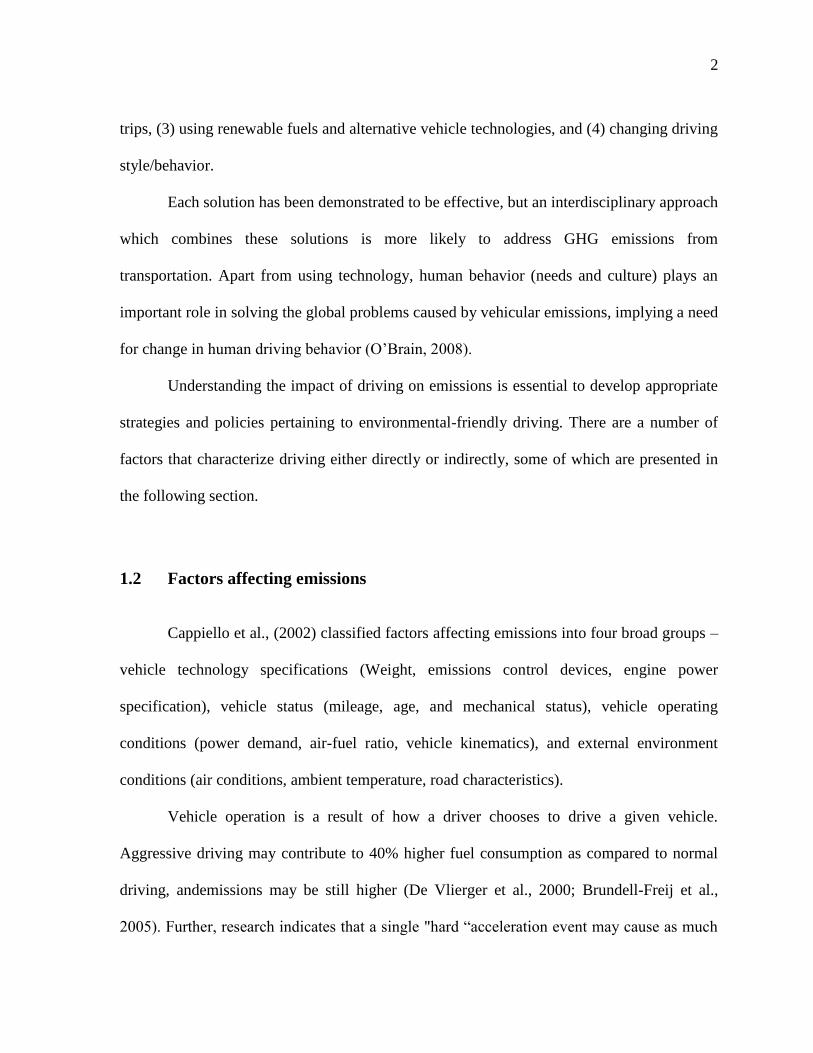
1.2 Factors affecting emissions

Cappiello et al., (2002) classified factors affecting emissions into four broad groups –

vehicle technology specifications (Weight, emissions control devices, engine power

specification), vehicle status (mileage, age, and mechanical status), vehicle operating

conditions (power demand, air-fuel ratio, vehicle kinematics), and external environment

conditions (air conditions, ambient temperature, road characteristics).

Vehicle operation is a result of how a driver chooses to drive a given vehicle.

Aggressive driving may contribute to 40% higher fuel consumption as compared to normal

driving, andemissions may be still higher (De Vlierger et al., 2000; Brundell-Freij et al.,

2005). Further, research indicates that a single "hard “acceleration event may cause as much

3

pollution as the rest of the trip (Guensler, 1993). Such findings have led to the adoption of

environmental friendly driving habits, some of which are presented in the next section.

1.3 Eco-driving

Eco-driving strategies pertain to driving in a more environment friendly manner in

order to reduce fuel consumption and emissions. According to eco-driving practices, small

changes in driving style can affect big overall savings in energy use and lowering fuel

consumption and emissions. Aggressive driving (speeding and braking) can lower gas

mileage by about 33 % on a highway and 5% on an urban road. For most vehicles, an

optimum speed at which fuel economy is highest is in the range of 35 to 55 mph (EPA,

2010). Each five mph above 60 mph can reduce fuel economy by 7%. Fuel economy is

highly correlated to emissions.

Optimizing driving habits can help reduce emissions and fuel consumption. Nissan

introduced the world‟s first eco-pedal to help reduce fuel consumption. They identified an

unfavorable region of acceleration where the emissions are significantly high. An eco-pedal

restricts the free flow pushing of the gas pedal and keeps the acceleration under a limit

thereby checking the emissions. In essence, it helps in smooth acceleration. When high

acceleration is needed, it is provided gradually. Nissan's internal research shows that driving

with eco-pedal is likely to reduce fuel consumption by 5-10% (Nissan, 2008). Based on the

many research findings on impact of driving on emissions and fuel consumption, several

programs have been initiated to propagate eco-driving. The examples include,

4

1.) EcoDriving USA (EcoDriving, 2011),

2.) Driving Change (Hickenlooper, 2011), and

3.) GreenRoad (GreenRoad, 2011)

These programs have been in effect for a while and claim to reduce fuel consumption

and carbon foot prints to the environment. The efficient driving habits include:

1.) Reducing idling

2.) Driving at speed close to speed limit

3.) Avoiding sudden hard accelerations

4.) Adopting smooth starts and stops

5.) Avoiding as much travel during off-peak hours as possible

6.) Taking the shortest route with the best roads

7.) Using cruise control

8.) Maintaining tires at the recommended air pressure

9.) Removing unwanted things from the vehicle to reduce its weight

The driver‟s behavior at a given traffic or road condition is generally termed as

driving behavior (or driver behavior). The next section elaborates on this further.

1.4 Driving behavior

Driving behavior is defined as any parameter or group of parameters, combination,

their derivatives or transformations that characterize the choice of speed, acceleration and

gear by a driver to accomplish the driving task (Ericsson, 2005). It can also be stated as an

5

attitude manifested in terms of acceleration, braking, cornering, lane handling and speed

handling (Greenroad, 2011). Transportation activities are identified on a micro-scale level as

driving behavior in this study. To implement appropriate strategies and policies that can help

in reducing emissions, it is essential to understand and model emissions as a function of

transportation activities or driving behavior.

1.5 Motivation for this work

The science of transportation of people and goods is an interdisciplinary subject.

Vehicular emissions depend on the road characteristics, driving behavior and the vehicle.

These factors are repeatedly being studied by transportation professionals, human factor

researchers and vehicle manufacturers.

The present research is aimed towards studying the effect of traffic control devices

and driving behavior on vehicular emissions and fuel economy at micro-scale level. Good

understanding of the impact of driving style on emissions would improve existing driving

style education programs (Mierlo et al., 2004). Although, aggregate comparisons have been

made (Holmén and Niemeier, 1998) across drivers, previous researchers have not modeled

driving behavior on a micro-scale level (second-by-second). This research is aimed towards

modeling driving behavior on second-to-second basis. Understanding driving behavior at

micro-scale level is likely to improve instantaneous emission models which are based on

aggregate measures.

Also, researchers have not compared traffic control devices in the light of driving

behavior parameters that affect emissions. A comparative study of driving behavior at most

6

common traffic control devices is the focus of this research. This is likely to enhance

modeling emissions at individual traffic control devices. The following section presents

objectives that served accomplish the purpose of this research study.

1.6 Research objectives and problem statement

The analysis presented in this research was done on three levels namely (1)

parameter-level, (2) intersection level, and (3) second-by-second level. The objectives

underlying these analyses are stated below.

1.) To explore existing and proposed parameters in terms of drivers and traffic control

devices.

2.) To compare driving behavior exhibited at different traffic control devices.

3.) To model and compare driving behavior of individual drivers on micro-scale level

(second-to-second basis). This objective was motivated by finding a unique driving

behavior model that can represent a typical driver. A driving behavior model can be

highly useful in quantifying emissions at a given traffic control device.

1.7 Research scope

The study explored driving behaviors corresponding to a mid-size passenger car on

the level of trips, traffic intersections, and a given geographical co-ordinate. The driving

behavior of four different drivers was studied in terms of various parameters that affected

vehicular emissions.

7

The research would help understand driving behavior and emissions at individual

traffic intersections. This would improve the present emissions models and emission

estimates and help in developing appropriate strategies for controlling emissions.

1.8 Organization of this dissertation

The dissertation is divided into seven chapters. The first Chapter introduces the

background of the research, factors affecting emissions, driving behavior and emissions. It

further describes the motivation and the research objectives and presents the scope of this

work. The second chapter summarizes previous research on driver behavior and emissions

analysis as well as emissions at different traffic devices. Chapter three contains data

collection methodology, study design and data preparation. Chapter four presents an

exploratory study on driving behavior parameters. Chapter five compares driving behavior

across various traffic control devices. In chapter six, individual driving behaviors are

modeled and compared across drivers. The last chapter (seven) summarizes the findings and

contributions of this study, discusses the assumptions, explains the limitations and challenges

faced, and presents recommendations for future research.

8

CHAPTER 2. Literature Review

This chapter summarizes studies on various aspects of driving behavior and its

relationship to emissions. In addition, driving behavior and emissions specific to traffic

control devices are also discussed.

2.1 Driving behavior and emissions

This section presents studies that correlate driving behavior with emissions. Past

researchers have shown that driving behavior (or vehicle operating mode) directly affects the

power required to operate a vehicle at a given state. Fuel consumption is highly correlated to

emissions. The higher the power demanded of the engine, the higher is the fuel combustion

leading to higher vehicular emissions. Emissions measured by a portable emissions

monitoring system (PEMS) have high variability from one run to another due to factors such

as engine condition, environmental condition and driving behavior (Rouphail et al., 2001).

Understanding and modeling driving behavior is likely to help researchers in evaluating

emissions more accurately and help in making appropriate policies for controlling vehicular

emissions.

Evans (1979) studied the effect of driver behavior on fuel consumption on urban

roads. Nine drivers including one with considerable experience and expertise in minimizing

fuel consumption were asked to drive on a route with vehicle equipped with vacuum gauge

fuel economy meter. The meter was divided into three regions namely green, orange and red

which indicated increased level of power use or fuel consumption. The objective of the

9

research was to contrast change in driving behavior due to traffic conditions and change due

to individual driving style. In order to capture specific driving behaviors, the subject drivers

were given seven instructions as stated below. They were asked to perform the following

task.

1) Drive as they would do under normal conditions

2) Minimize trip time

3) Use vigorous acceleration and deceleration

4) Minimize fuel consumption by taking feedback from the fuel meter placed in the

dashboard area

5) Maintain fuel economy meter in green region

6) Maintain fuel economy meter in green or orange region, and

7) Drive like a hypothetical, very cautious driver

The researcher found that for every 1% increment in trip time, the fuel consumption

increased by about 1.1 %. Research showed that expert drivers can save fuel without

changing trip time by making adjustments to their driving behavior in term of maintaining a

particular speed and acceleration. The researcher also found it challenging to develop a

„perfect‟ fuel meter that would enable the driver to achieve optimum fuel economy in real-

time.

Wang et al. (2008) studied driving behavior and developed driving cycle for Chinese

cities. Driving cycle, as mentioned earlier, is a standard speed profile, which represents

typical driving behavior for a given road class and drivers. Eleven cities of various sizes and

10

geographical locations were selected for the study. On-road speed profiles were recorded

using car chase technique on freeways, arterials and local roads. Professional drivers were

asked to follow traffic in specific routes. The vehicle used was instrumented with a GPS and

a speed sensor. Two sets of equipment were used to ensure high quality data. Data were

collected during morning peak hours (7:30–9:00), afternoon off-peak hours (11:00–13:00),

and evening peak hours (17:00–18:30). To estimate the characteristic of the entire traffic, the

authors derived traffic adjustment factors based on road type, peak hours, traffic volume,

road length and average speed on the road. Eleven driving behavior parameters were derived

from the time-speed traces. These include (1) average speed, (2) average running speed

(average speed after removing idling events), (3) average acceleration ,(4) average

deceleration, (5) percent of time in idling mode, (6) percent of time in accelerating, (7),

percentage of time cruising, (8) percent of time in decelerating, (9) relative positive

acceleration, (10) positive acceleration kinetic energy, and (10) the frequency of decelerating

phase after an acceleration phase for every 100 meter driven. Vehicle driving pattern was

found to be dependent on the size of city, local road characteristics and individual driving

behavior. The driving behavior pertaining to Chinese cities was found to be significantly

different from the driving behavior corresponding to European and US driving cycles. This

entails that driving cycle for European and US driving cycle cannot be used for

characterizing driving behavior in Chinese cities including the large ones. Based on the

longer duration of cruising and acceleration mode (over 83%), it was found that driving in

Shanghai, China and Chengdu, China involved high percentage of acceleration and hard

brakes. Shanghai and Chengdu were also associated with aggressive driving as depicted by

11

high acceleration and deceleration measurements. Driving in small Chinese cities was found

to be less aggressive.

Holmén and Niemeier (1998) conducted a field study of 24 drivers to study the effect

of acceleration events on real-world vehicle emissions. They found that the variability

associated with driving behavior produced significantly different tail pipe emissions. There

were significant variations in CO and NOx emissions among the 24 drivers under similar test

route, traffic density and vehicle type. They found that driving patterns were dependent on

the intensity of vehicle operation within a given mode.

Ericsson (2000) studied the variability in urban driving behavior in light of driver,

street environment and traffic conditions. Twelve university employees were chosen to drive

a car instrumented with a data-logger that registered vehicle speed every 1/10th

of a second.

The route consisted of a loop from a residential area to the city center and back on the same

road. Street type, peak hour/off-peak hour and gender were considered as fixed effects while

driver was taken as a random factor. The driving behavior of each driver was assessed using

26 parameters divided into three categories namely level measures, oscillation measures and

distribution measures. Level measures consisted of means and standard deviations of speed

and acceleration. Oscillation measures comprised of relative positive acceleration (RPA) and

the frequency of occurrence of a particular ratio of maximum speed to min speed. On the

other hand, distribution measures consisted of various intervals of speed, acceleration and

deceleration. The marginal effect of each of the driving behavior parameters were studied

for driver, street environment and traffic conditions (peak/off-peak hours). The study was

conducted to compare driving behavior between and within different street types, drivers and

traffic conditions. Driving behavior showed very significant differences between street type

12

and driver for in terms of all parameters. The effect of street type was generally higher than

the driver effect. Average speed and average deceleration were found to lower at peak hour

conditions. Men were found to drive at higher average acceleration levels. According to the

researcher, the most important driving behavior parameters were relative positive

acceleration, frequency of occurrence of maximum speed/minimum speed to be greater than

2 per 100 m, percentage of time when acceleration exceed 1.5 m/s2, percentage of time when

deceleration was about -1.5 to -2.5 m/s2, and percentage of time speed below 15 km/h (~ 10

mph).

Ericsson (2001) attempted to find independent driving behavior parameters that can

explain a large variability in emissions and fuel consumption. To collect vehicle activity and

driving behavior data, five passenger cars of different sizes and performances were equipped

with a data-logger and driven on roads in an average sized Swedish city. A total of 2550

journeys and 18945 km of data were collected. Subject drivers were chosen from 30 families

in the city of Vasteras, Sweden. As revealed by the families, 45 different drivers drove the

vehicles. Driving behavior was attributed to street type, street function, street width, traffic

flow and codes for location in city (central, semi-central, peripheral). A total of 62 different

driving behavior parameters were defined depending on which of the attributed values

changed. These parameters measure distribution of speed, acceleration and deceleration,

occurrence of stops, maximum speed/minimum speed, duration of time driving at a given

gear, and vehicle power. The researcher found that many of the driving behavior parameters

are correlated. Factor analysis was performed, which reduced the number of parameters to 16

independent measures which the researcher called typical parameters. Factor analysis is a

method of constructing new variables from the linear combination of the original variables

13

such that the new variables have negligible correlation among them. Emissions and fuel

consumption were estimated for the chosen vehicles using Swedish emissions models

(VETO Rototest models). The estimated emissions and fuel consumption were then modeled

using regression on the typical factors. Of the sixteen factors, nine factors pertaining to

power demand, gear-changing pattern and certain speed range had considerable effect on

emissions. Specifically, fuel consumption was affected by factors corresponding to high and

moderate power demand, stops, speed oscillation, extreme acceleration, and high speed and

moderate speed at gear two and three. Emissions of HC were primarily dependent on

acceleration with high power demand and extreme acceleration. NOx emissions were mainly

affected by acceleration with high power demand, extreme acceleration, engine speed > 3500

rpm and late gear changing from gears two and three.

Nam et al. (2003) compared real-world CO, THC (C3H8), NO, and CO2 emissions

with modeled estimates at different driver aggressiveness. The authors used a PEMS to

measure real-time emissions (above gases), travel times and vehicle kinematics through a

busy road network in southeast Michigan. Emissions were also estimated using an integrated

framework of Comprehensive Modal Emissions Modal (CMEM) and a microscopic traffic

model VISSIM. The emissions model was calibrated with on-road data using a

dynamometer. The researchers used root mean square of power factor (2*speed*acceleration)

as a measure of driver aggresivity. For each trip, driver aggresivity was computed. They

found that aggressive driving produced significantly higher emissions as shown in Table 2.1.

14

Table 2.1: Emissions for normal and aggressive driving (Nam et al., 2003)

Measurement

Model

estimates

Driving Normal Aggressive VISSIM

Travel time (sec) 1011 1031 974

Aggressivity (kmph2/s) 95.7 116.1 83.4

Fuel (g/mile) 154 165.1 135.5

CO2 (g/mile) 488.7 521.4 428.9

CO (g/mile) 0.25 2.00 0.41

HC*100 (g/mile) 0.04 2.41 0.89

NOx (g/mile) 0.52 0.67 0.31

Wahab et al. (2007) studied brake pedal and gas pedal pressure of the driver to

understand the driver behavior under different environmental conditions. The driving data

was taken from In-car Signal Corpus hosted in Center for Integrated Acoustic Information

Research (CIAIR), Nagoya University, Japan. Stop-and-go-segments were extracted since

they contain a good percentage of acceleration and deceleration behaviors. New parameters

were derived by taking the first derivatives of gas pedal pressure and brake pedal pressure.

The researcher used four driving behavior parameters for analysis. These parameters, brake

pedal and gas pedal pressure and their derivatives, were transformed to frequency domain by

deriving the power spectral density. The authors used Gaussian mixture models (GMM) to

analyze the brake and gas pedal pressure plots (mesh and contour plots) of the individual

drivers. They found that these plots were unique for each driver proposed that this method

can be extended to predict sequences of individual driving behaviors. Driving behavior

parameters in various studies is listed in Table 2.2 along with reasons why they are

important.

15

Table 2.2: Driving Parameters from literature

Driving Parameters Why are they important? References

Mean speed Central tendency of motion (Kuhler and

Karsens,1978)

Mean driving speed Central tendency of motion (Kuhler and

Karsens,1978;

André,1996)

Mean acceleration Acceleration behavior (Kuhler and

Karsens,1978)

Mean deceleration Deceleration behavior (Kuhler and

Karsens,1978)

Mean driving duration Average speed maintained (Kuhler and

Karsens,1978;

André,1996)

Mean number of acceleration

and deceleration changes in a

trip

frequency of brake pedal and gas

pedal use

(Kuhler and

Karsens,1978;

André,1996)

Proportion of stand still time

(v< 3 km/h, |a| <0.1 m/s2)

Correlated with duration of idling (Kuhler and

Karsens,1978)

Proportion of acceleration time Frequency of acceleration (Kuhler and

Karsens,1978)

Proportion of deceleration

time

Frequency of acceleration (Kuhler and

Karsens,1978)

Acceleration standard

deviation

Change in frequency of acceleration (André,1996)

Positive kinetic energy Vehicle energy demand (André,1996)

Number of stops per km Number of acceleration and

deceleration phases

(André,1996)

Relative and joint distribution

of speed, acceleration and

deceleration

Adaptation to maintain a given

speed and acceleration

(André,1996)

16

Inertial power

(acceleration x speed)

Adaptation to overcome drag force (Fomunung et al. ,1999)

Drag power

(acceleration x speed2)

Found to be highly correlated with

me and fuel consumption for heavy

duty vehicles

(NAP, 2000)

Relative positive acceleration Measure of stress taken by the

engine

(Weijer,1997; Mierlo, et

al.,2004; Ericsson, 2000)

RPM Central tendency of motion (Mierlo, et al.,2004)

2.1.1 Summary (Driving behavior and emissions)

Vehicular emissions are found to be highly dependent on how much energy (in the

form of fuel combustion) is demanded of the engine. Amount of emissions are dependent on

diver activities as quantified by the four common driving modes namely – cruise, idling,

acceleration and deceleration. Studies outlined above shows that emissions is highly

correlated to driving behavior. High speed and acceleration mode are especially responsible

for peak emissions. Several driving behavior parameters have been utilized in the literature to

explain driving behavior.

2.2 Emissions at various traffic control devices

Emissions at a road intersection were found to be significantly higher than that at

mid-block sections of the road. This is because intersections tend to make drivers slow down

or stop. This entails the driver to accelerate to attain the flow speed. The following studies

quantify and compare emissions at traffic intersections.

Ahn el al. (2009) evaluated the energy and environmental impacts of installing a

roundabout, all-way-stop, or a traffic signal at an intersection that was an alternative access

17

point to Washington Dulles Airport. The intersection experienced high traffic volume during

peak hours. Through simulation, the researchers compared emissions at the traffic

intersection by assuming it to be either a roundabout, a stop control (two way stop control) or

a traffic signal. They used INTEGRATION and VISSIM to simulate large number of

deceleration and acceleration events corresponding to the three traffic control devices. The

authors also estimated the second by second emissions and fuel consumption using VT-

Micro model and the Comprehensive Modal Emissions Model (CMEM). The roundabout

was found to be efficient as long as the traffic demand increased by 50 percent. However,

beyond that, the roundabout produced substantial increase in delay while traffic signal was

most efficient. With VISSIM and VT-Micro model, fuel consumption was found to increase

by 13 % and 8% when the stop sign control was substituted with proposed roundabout or a

traffic signal, respectively. CMEM estimated that fuel consumption increased by 18% when

stop sign control was replaced by a roundabout. The roundabout produced 155%, 203%,

38%, and 10% higher HC, CO, NOx, and CO2 emissions, respectively. On the other hand,

HC, CO, NOx, and CO2 emissions increased by 80%, 108%, 28%, and 8% respectively at the

traffic signal based on VT-Micro model estimates. According to CMEM model HC, CO,

NOx, and CO2 emissions increased by 344%, 456%, 95%, and 9%, respectively roundabout

was installed instead of the stop control. Results also showed that increase in emissions and

fuel consumption was greater for roundabout than for traffic signal.

Coelho, et al. (2006) studied the environmental impact of a single lane roundabouts

located in Lisbon (Portugal) and Raleigh (North Carolina, US). They videotaped the site and

extracted queue length, time gap between successive acceleration-deceleration cycles, and

the number of times the vehicle stopped before entering the roundabout circle. Real-world

18

speed profiles for typical stop and go conditions were obtained from repeated runs at several

single lane roundabouts in the region of Lisbon. A microwave Doppler sensor was used for

measuring entrance speed of various vehicles. The researchers recorded stop and go

behavior, on-road emissions and synthesized speed profiles using traffic volume and

conflicting volume (or circulating volume) which are correlated with queue length. Based on

intensive empirical measurements the researchers identified three typical speed profiles

(Figure 2.1) that can be observed at a roundabout. The probability of occurrence of each of

the profiles was modeled using approaching traffic volume and circulating traffic volume.

The proportion of time the vehicle experienced profile I, II and III were found to be 43%,

36% and 21% respectively. VSP was computed from speed profiles and then based on VSP

bins and emissions lookup table (North Carolina State University, 2002; Frey et al., 2003)

NOx, HC, CO, CO2 and PM emissions were estimated.

They found that the region of influence where vehicles accelerate back to free flow

speed (after encountering traffic intersection) was important in terms of understanding its

relative impact on total emissions. About 25 % of total emissions were found to have come

from this region of acceleration. Emissions were found to increase monotonically with free

flow speed (speed limit outside the influence of roundabout) beyond the region of

acceleration. Emissions were found to increase as the difference between free flow speed and

circulating speed became larger.

2.2.1 Summary (emissions at traffic control devices)

Previous research shows that emissions at various traffic control devices varied across

traffic control devices. This is due to the difference in driving behavior when drivers try to

19

adjust their speeds to traverse various sections of the road or intersections. It was also found

that emissions at these traffic control devices were highly dependent on traffic conditions.

Figure 2.1: Typical speed profiles at a roundabout (Coelho, et al., 2006)

2.3 Contributions of the present study

This dissertation extends the finding and methods to study driving behavior across

drivers and traffic control devices. Driving at a traffic control device is a characteristic of

individual driving behavior. In this dissertation, we studied individual driving behavior at

traffic control devices to closely examine its impact on emissions. Specifically, the

dissertation has the following contributions.

20

1.) Wahab et al. (2007) quantified driving behavior by the amount of pressure the driver

applied on the gas pedal and brake pedal. In this dissertation, this concept of gas pedal

pressure and brake pedal pressure was used to study driving behavior and its impact on

emissions. Variables quantifying gas pedal pressure and brake pedal pressure were

derived from acceleration.

2.) Emissions at traffic intersections are significantly different from those at the mid-block

sections of the road. Traffic control devices force the drivers to slow down (or stop) and

then accelerate which results in higher emissions. Researchers have studied driving

behavior and emissions for different road types (Ericsson, 2000) but they did not compare

driving behavior across traffic control devices. Some studies compared emissions and

fuel consumption but did not adequately explain how they are correlated to driving

behavior at traffic control devices. In other words, this dissertation studies on driving

behavior in the light of traffic control devices while taking the driver as a random

variable.

3.) In general, studies have compared driving behavior of different drivers in terms of

aggregate measures. In this dissertation, an attempt was made to compare driving

behavior on a micro-scale (second-by-second) level. This is important for identifying

hotspots where a typical driver or a certain group of driver operates the vehicle

differently so as to produce significantly high emissions. Aggregation takes away the

information on instantaneous driving behavior. Driving behavior of the overall trip tends

to average out and details regarding acceleration and deceleration behavior are not well

segregated. For example, we may consider a driver who accelerates hard to change lanes

21

but slows down smoothly at the traffic control devices. Taking average value of such a

trip tends to hide the high acceleration event. Instantaneous models require quantification

of driving behavior at high resolution (in time and space). This dissertation, attempted to

further the research by comparing driving behavior at roundabout, all-way-stop, and

traffic signal. Driving behavior like acceleration and deceleration in terms of their

duration and intensity can be well captured at the traffic intersections where it is

unavoidable to observe these behaviors. This study modeled and compared speed profiles

across drivers in order to validate the assumption that driving behavior differ across

drivers and that the driver must be treated as a random variable.

22

CHAPTER 3. Data Collection and Data Preparation

3.1 Research outline and data collection

Data collection is a critical step in any research process since it is highly dependent

on the objective of the study. The broad objective of the study was to explore driving

behavior and emissions at traffic control devices: roundabout, all-way-stop, traffic signal. In

order to achieve this objective, on-road emissions tests were performed and driving behavior

of four drivers were measured and analyzed.

This chapter gives a detailed description of data collection procedures, and data

preparation or preprocessing required for analyzing the collected data. The following section

describes the data collection processes: selection of appropriate route, vehicle, instrument,

and study period. This is followed by data preparation which comprised of extracting

relevant information from the raw data, defining new variables, removing outliers and

preparing the final data tables required for specific analysis in the upcoming chapters.

3.2 Data collection and study design

Vehicular emissions highly depend on the study period and traffic conditions (Ahn et

al. 2002), test route (Ropkins et al., 2007), vehicle (Wenzel and Singer, 2000), and driver (Yu

and Qiao, 2004). In addition, vehicular emissions are also affected by the type of traffic

control device encountered at a traffic intersection (Coelho et al., 2006; Mandavilli et al.,

2008; Ahn el al., 2009). Therefore, an appropriately chosen test period, test route, test

23

vehicle and subject drivers are needed. The following sections elaborate on these important

aspects of data collection protocol.

3.2.1 Study route

The study was aimed at understanding driving behavior at various traffic control

devices. Several potential test sites were evaluated in this regard. Eventually, a corridor along

Douglas Avenue (Urbandale, IA), a minor arterial, was chosen as the test route (Figure 3.1).

This corridor was chosen as it has all the three traffic control devices in a row. The speed

limit on the route was 35 mph except for the roundabout circle where it was 15 mph. Same

speed limit throughout the route offered similar conditions for comparing driving behavior

across traffic control devices. A pilot study was conducted on the chosen route, and this

provided insight into the traffic and road environment the experiment drivers would

encounter. Douglas Avenue runs east to west and passes over the interstate I-35 while

connecting with it through a partial cloverleaf interchange.

The chosen corridor is a paved four-lane road (median separated) except on the west

side of the all-way-stop where it changes to a two-lane road. The route is comprised of a

traffic signal, a roundabout (radius ≈1780 ft.), an all-way-stop, curve section and a tangent

section (length ≈1.62 miles). The length of the tangent section and curve section were 1.62

and 0.5 miles respectively. The total length of the test route was three miles.

24

Figure 3.1: The study route chosen for data collection (Map © 2011 Google)

To indicate different portions of driving, the following terms were defined.

1.) Loop: A loop of driving implied driving from the east end of the route to the west end

and back.

2.) Trip: A trip was defined as driving from one end to another. A loop consisted of two

trips.

3.) Trip-part: A trip-part denoted the portion of a trip that was in the region of influence

of a traffic intersection or traffic control device.

The next section describes the vehicle and equipment used for data collection on the

above test route.

3.2.2 Portable Emissions Monitoring System (PEMS)

In general, tail-pipe emissions can be measured using two methods namely on-road

testing and dynamometer testing. The former entails instrumenting a vehicle and measuring

the emissions while it is in-use on the road. The latter is a laboratory set up where the vehicle

25

is made to mimic a standard speed/acceleration profile called driving cycle. This standard

driving cycle is a sequence of many driving behavior events. It is a representative of driving

behavior for a given vehicle and road type. A portable emissions monitoring system (PEMS)

was used in this study for measuring and recording emissions and vehicle activity data. This

equipment has the following advantages.

1.) Time effective: It can be hooked up in 20-30 minutes for hours of testing whereas

using a dynamometer is time consuming. Setting up the equipment consists of

connecting the PEMS to a power source (an external battery placed inside the moving

vehicle), placing the sample probe in the exhaust, routing exhaust lines, and

connecting on-board sensors to various locations of the engine.

2.) Wider deployment: A wide range of vehicles can be tested at reasonable cost and

time. PEMS has been used on both on-road and off-road vehicles (Frey et al., 2005).

3.) Testing various scenarios: It measures real world driving pertaining to a specific

road, vehicle and driver. For this reason the PEMS is helpful in identifying high

emissions spots, in recording hard acceleration events, aggressive driving and other

driving behaviors (Holmen et al., 1997; Nam et al., 2003; Yu and Qiao, 2004) on a

second-to-second basis. It is also shown to be a good tool in assessing the impact of

traffic control on emissions (Frey, 2000) or comparing emissions across different

routes (Ropkins et al., 2007). The PEMS can also be an effective device in comparing

emissions at different road grades (Frey et al., 1997) and in assessing the impact of

transportation improvements on emissions (Rouphail et al., 2001; Unal et al., 2003).

26

Further, PEMS can also be used for testing renewable fuels or power sources (Frey et

al. 2007).

With all the above advantages, however, PEMS data is comparatively less reliable for

standardizing emission factors due to lack of repeatability. Dynamometer measurements are

mandatory for quantifying emission factors and developing environmental policies.

However, PEMS data when successfully validated using a dynamometer testing, can be very

useful since it also records factors that affect emissions.

The PEMS (Figure 3.2) used in this study was the Axion system manufactured by

Clean Air Technologies Inc. The emissions measured by the PEMS are hot-stabilized oxides

of nitrogen (NOx), hydrocarbon (HC), carbon monoxide (CO), carbon dioxide (CO2) and

particulate matters PM10.

The PEMS records emissions and engine parameters (rpm, intake air temperature and

manifold absolute pressure) along with geographic information (latitude, longitude, bearing

and altitude) using a GPS. The emissions, the engine parameters and geographic information

are synchronized on a second-to-second basis.

Concentration (mass/second) of emissions is estimated using engine-RPM, intake air

temperature, manifold absolute pressure and mass of emissions per unit volume of the

exhaust. This also takes into account the user-supplied fuel composition. The manifold

absolute pressure transforms changes in engine speed and load into electrical signals which

control the flow of fuel into the engine. Engine rpm and intake air temperature provide

information on engine stress.

27

Figure 3.2: Axion (Portable Emissions Monitoring System, Source: www.cleanairt.com)

The system consists of two gas analyzers which alternatively perform zeroing – a

method in which each analyzer calibrates itself with the ambient air away from the exhaust

air. The values corresponding to the active (sampling from the tail pipe) analyzer are

recorded. When both the analyzers are active, average values are logged.

We used PEMS for measuring vehicle activities and emissions on a single test vehicle

which is discussed in next section.

3.2.3 Test vehicle

Emissions tests were conducted on a 2005 Ford Taurus, a mid-size passenger car. The

test vehicle operated on gasoline with automatic transmission feature. The objective of the

study was to understand driving behavior, and therefore it was assumed that each driver

would drive any other mid-size passenger car in a similar manner. A single vehicle was used

to reduce the possible variability in emissions due to the use of different vehicles (Frey et al,

2010). This test vehicle was driven by subject drivers who are described in the next section.

28

3.2.4 Subject drivers

Four graduate students at Iowa State University were chosen as subjects drivers for

the study. Two were male and two female, and their age ranged from 20 to 25 years. Each

had a minimum of three years of experience with driving and was familiar with US road and

traffic conditions and regulations.

3.2.5 Data collection period

A total of four days of data were collected. This included morning and afternoon peak

and off-peak hours. The morning and afternoon peak hours were assumed to be from 7 to 9

am and from 5 to 7 pm respectively. /The morning and afternoon off-peak hours were from 9

to 11 am and from 3 to 5 pm. Two drivers drove from 7 to 11 am on 13 and 20th April 2010

and the other two drove from 3 to7 pm on 7th and 14th April 2010. The data collection

schedule is summarized in Table 3.1.

Table 3.1: Data collection schedule

Morning

peak

Morning

off-peak

Afternoon

peak

Afternoon

off-peak

Date => 13 and 20 April 2010 7 and 14 April 2010

Time => 7 to 9 am 9 to 11 am 3 to 5 pm 5 to 7 pm

Driver-1 X X

Driver-2 X X

Driver-3 X X

Driver-4 X X

29

3.3 Test protocol

On the day of data collection the vehicle was equipped with PEMS at the gas station

located near the east end (shown as red balloon point A in Figure-3.1). Two of the four

drivers and a data collector would sit in the car at driver and passenger seats respectively. A

given driver would drive from the east end to the west end of the corridor and back thus

completing a loop. After few loops of driving the subject drivers would switch places to

prevent boredom and fatigue which may affect their natural driving. On an average, each

driver made 25 trips. A total of 109 trips of data were collected. This comprised 16 hours of

driving. The duties of the data collector included,

1.) Making sure that the PEMS was working normally and that it was fastened tight to

the vehicle. While on the road, the PEMS is subjected to motion and vibrations which

can lead to equipment malfunction and may also render the data invalid.

2.) Recording queue position while the drivers stopped and waited for their turn at the

traffic intersections.

3.) Making a qualitative assessment of the traffic flow, and recording abnormal traffic

conditions, if any.

Once the data were collected, these were preprocessed for analysis and interpretation.

The next section deals with data preparation which includes data cleaning, variable

extraction, and defining new variables.

30

3.4 Data preparation

PEMS provides raw data in the form of comma separated values (csv) files. The data

were imported into Excel (2007). Some variables were in the form of strings and were

therefore transformed to numbers. The data were processed and a quality assurance process

was performed. The steps taken to address inappropriate data and to process the data into the

final format for analysis are described below.

3.4.1 Eliminating unwanted columns in data sheet

In order to simplify the data processing and analysis, variables such as altitude, and

those related to raw gas analyzers data were removed since they were not needed to meet the

objective of this study.

3.4.2 Inserting categorical variables

In order to segregate observations corresponding to individual driver, trip number,

date and time of testing and direction of travel, new categorical variables were defined for

each spreadsheet file. These variables were “Driver”, “TripID”, “DT”, and “Dir”. PEMS

records the bearing of the moving vehicle. The variable “Dir” implying direction of travel

was obtained using the bearing values recorded by PEMS. A bearing of more than 180o

implied west bound.

31

3.4.3 Removing rows with abnormal observations

Some observations had negative and exceptionally high emissions values (e.g. > 100

g/s). Negative values may appear due to very low value of the given emissions, an error in

the equipment (PEMS), or because of unusually high concentrations in the ambient air which

was used as a baseline. Identification and removal of observations was performed in R

(Version 2.11.1).

3.4.4 Defining new parameters and variables

Several new variables were created using existing variables as shown in Table 3.2.

Acceleration was calculated as rate of change of speed. Jerk, the rate of change of

acceleration, was used as a measure of hard acceleration. Jerk has been used by many

researchers to quantify aggressive driving behavior (North et al., 2006; Bagdadi and

Varheliyi, 2011). Vehicle specific power (VSP) is a function of speed, acceleration and road

grade. It is shown to explain a good percentage of variability in emissions (Jiménez-Palacios,

1999; Frey, 2002; Nam, 2003). Two major emissions models namely MOVES and CMEM

utilize VSP for characterizing emissions. Road grade was assumed to be zero on the given

route. Therefore, in the present context VSP was only a function of speed and acceleration.

The variables gaspad and brakepad denoted the gas pedal use and brake pedal use

respectively. These variables, computed from acceleration, were effective in segregating

acceleration and deceleration behavior at a given second.

32

3.4.5 Data Merging

After cleaning the data and defining relevant variables, data from various

drivers/trips/days were merged into a single datasheet for easy editing, querying and

analyzing.

3.4.6 Assigning roadway and traffic control variables

The Manual on Uniform Traffic Control Devices (MUTCD) defines a traffic control

device as “a sign, signal, marking, or other device used to regulate, warn, or guide traffic,

placed on, over, or adjacent to a street, highway, pedestrian facility, or shared-use path by

authority of a public agency having jurisdiction” (MUTCD, 2009)

In this dissertation, driving behaviors at the three traffic control devices namely

roundabout (RDA), all-way-stop (AWS), and traffic signal (TS) were studied. A new

variable called “TrafficD” was defined to indicate a traffic control device present at a given

section of the route. This section called “region of influence” was identified using a GIS

package (ArcMap 9.3).

On an average, the drivers entered a deceleration phase about 500 ft. upstream of a

traffic control device. Similarly, drivers on an average utilized 500 ft. to accelerate to the free

flow speed of the corridor. Based on this the region 500 ft. upstream and 500 ft. downstream

of a given traffic control device was labeled accordingly (RDA for roundabout, AWS for all-

way-stop, or TS for traffic signal). Figure 3.3 shows the route (green) with region of

influence of respective traffic control devices highlighted in brown.

33

Table 3.2: Primary variables/parameters used in data analysis

Variable Names Variables Remark

NOx, HC, CO2, CO and PM Nitrogen oxides, hydrocarbons, carbon

dioxide, carbon monoxide

Tail pipe emissions

RPM, Temp, MAP Rotation per minute, intake air

temperature, manifold absolute

pressure

Give an idea of how much stress in put

on the engine. It transforms to fuel

demand.

Speed Speed in miles per hour

accl

acceleration =

in mph/s

Isn‟t acceleration given by the PEMS?

Why calculate it yourself?

jerk jerk

Indicator of driver aggressiveness

VSP Vehicle specific power

Where, v= speed in m/s and

a= acceleration in m/s2

This variable is highly correlated with

emissions (Jimenez-Palacios,1999)

gaspad Positive acceleration

= accl , if accl>0

=0, otherwise

Gas pedal use (indicator for

acceleration behavior)

brakepad negative acceleration

=abs(accl) , if accl<0

=0, otherwise

brake pedal use (indicator for

deceleration behavior)

DT Date and time

peakhour Peak or off-peak hours

TrafficD Traffic devices (Roundabout, all-way-

stop, Traffic signal) abbreviated as

RDA, AWS, TS (or TS128)

Driver Denoted as D1, D2, D3 and D4

34

Figure 3.3: Route showing the region of influence (top figure) of the traffic control devices

For the purpose of data preparation, data manipulation, data analysis and

reporting/post processing, more than 1000 lines of code were written in R (version 2.11.1).

Excel 2007/2010 was used for data management. The following section describes the final

datasets used for analysis.

3.5 Final dataset used for analysis

Data analysis was carried out using various driving behavior parameters. Table 3.2

shows primary driving behavior parameters (also called primary parameters). The divers

drove for a total of 16 hours. This comprised of 38,000 observations of primary parameters.

The secondary driving behavior parameters (also called secondary parameters) as shown in

Table 3.3 were obtained by summarizing primary parameters and their combinations over

trip-parts (region of influence of traffic control devices). These parameters were used by

many researchers for characterizing driving cycles (Tong and Hung, 2010; Barlow et al.,

2009). For a given trip, a driver encountered each traffic control device (roundabout, all-way-

35

stop and traffic signal) on single occasion. Therefore, in 109 trips, 327 (3 x 109) trip-parts

were recorded. The number of rows of secondary parameters was 327.

Table 3.3: Trip-part summarized variables

Driving

behavior

parameter Definition (units)

Relevance

v_min

minimum speed for the whole trip

(mph)

Speed

behavior

v_avg average speed (mph)

vrun_avg

average running speed (excluding

observations with idling operation)

(mph)

v_max maximum speed (mph)

RMSs root mean square speed (mph/s)

N is the number of seconds of data

a_avg average acceleration (mph/s) Speed

change

behavior d_avg average deceleration (mph/s)

j_avg average jerk (mph/s)

RMSa

root mean square acceleration

(mph/s)

ADS

Number of acceleration/deceleration

shifts (number of speed changes)

RPA relative positive acceleration (mph/s)

trip_len trip length (s) Duration of trip Time spent

in each

mode Pi percent of time in idling mode (%) Percentage of time when speed =0

Pa

percent of time in accelerating mode

(%) Percentage of time when acceleration ≥ 0.1 m/s2

Pc percent of time in cruise mode (%)

Percentage of time when speed < 5 m/s and

-0.1 m/s2 < acceleration < 0.1 m/s

2

Pd

percent of time in decelerating mode

(%)

Percentage of time when speed < 5 m/s and

-0.1 m/s2 < acceleration < 0.1 m/s

2

PKE positive kinetic energy (mph/s)

Where vf and vi are the final and initial speeds,

respectively, in an individual acceleration phase

and x is the total travel distance

Energy

gained or

utilized

VSP_avg

Average value for vehicle specific

power (m2/s

2)

36

Data analysis was carried out at three levels namely parameter level, trip-part level

and micro-scale (second-by-second) level. Dataset corresponding to each level was described

as follows. Table 3.4 shows summary of the analysis.

1.) Exploring individual parameters: In this case, distributions of driving behavior

parameters were explored to compare driving behaviors across drivers and the traffic

control devices. For analysis pertaining to drivers, primary parameters were used whereas

for analysis on traffic control devices, both primary and secondary parameters were used.

Detailed analysis is documented in Chapter-4.

2.) Comparing traffic control devices: In this analysis, driving behavior at roundabout was

compared with that of all-way-stop and traffic control devices. In this case, secondary

parameters used for conducting MANOVA with traffic control device as explanatory

variable. Chapter -5 gives the details of this analysis.

3.) Second-by-second data: Second-by-second speed data at roundabout was used for

analysis. The speed profiles of drivers at the roundabout were modeled using hierarchical

Bayesian regression. The complete analysis is presented in Chaper-6.

37

Table 3.4: Summary of analysis done in future chapter

Analysis

level

Data Driving behavior

parameters

Objective Analysis

Parameter

level

All observations Speed,

acceleration, VSP,

gaspad, brakepad

Understanding

parameters that

quantify driving

behavior

Exploring the

frequency

distributions of

driving behavior

parameters

Trip-part

level

Driving behavior

parameters summarized

at each traffic control

devices

Parameters

derived primarily

from speed, and

acceleration

(These parameters

are used for

defining standard

driving cycles)

Comparing driving

behavior at different

traffic control

devices

Performing

MANOVA

Second-by-

second level

Second by second speed

profiles of each driver

Speed profile at

the roundabout

Comparing driving

behavior among

drivers

Developing

Hierarchical

Bayesian

regression model

38

CHAPTER 4. Study of Driving Parameters

4.1 Background and objectives:

The main objective of this dissertation is to study emissions in the light of driving

behavior and traffic control devices. Previous researchers have identified various parameters

that can quantify driving behavior at different levels. In this regard, this chapter explores few

of these driving parameters to quantify and contrast driving behavior across individual

drivers and across traffic control devices.

4.2 Data used in this analysis

In this chapter, exploration was done to explore if direction of travel and time of the

day had any influence on driving behavior. Then, driving behavior was studied across drivers

through speed (mph), acceleration (mph/s), VSP (W/kg), and jerk (mph/s2). In addition,

explored two new parameters gaspad (mph/s) and brakepad (mph/s) were also explored to

assess how well they can explain variability in driving behavior.

Driving behavior across the three traffic control devices (roundabout, all-way-stop

and traffic signal) was studied instantaneous speed, acceleration, “gaspad” and, “brakepad”.

These variables represented instantaneous driving behavior. Additionally, we studied driving

behavior in terms of positive kinetic energy (PKE), number of acceleration/deceleration

shifts (ADS), relative positive acceleration (RPA), and VSP (m2/s

2) where each one was

aggregated over the area of influence of the respective traffic control device. These variables

39

represented aggregate driving behavior. In this chapter, we based our conclusions on

observations; no statistical tests were performed.

4.3 Observatory study

Apart from the vehicle type, driving behavior is likely to differ by traffic volume

(correlated by time of the day), road geometry, individual driving habits and traffic control

devices (roundabout, all-way-stop, traffic signals, curves and tangents). The following

sections describes each of the above four characteristics that impacts driving behavior.

4.3.1 Time of the day and direction of travel

In this study, we collected data for both peak (7am to 9am and 5pm to7pm) and off-

peak (9am to 11am and 3pm to 5pm) hours. Driving behavior quantified as speed, VSP,

“gaspad” and “brakepad” was comparable between peak and off-peak hours (Figure 4.1).

This may be because of low volumes or similar volumes in both the time periods. Ericsson

(2000) found that difference in emission levels between peak and off-peak hours were not

significantly different for less congested roads.

Similarly, driving behavior was comparable between both the directions of approach

(Figure 4.2). This may like be due to similar road characteristic in both directions. This was

also observed by the data collector who noted the queue positions at the intersections and in

most cases the vehicle was at the beginning of the queue. This supported combining data in

both directions. East bound trips were not distinguished from west bound trip in future

chapters. The small differences seen in the graphs (Figure 4.1 - 4.2) were not significant.

40

Figure 4.1: Driving behavior variable for peak and off-peak hours

Figure 4.2: Driving behavior variable for east and west bound driving

Since driving behavior for different time of the day and direction of travel was not

considerably different, we combined the data and performed an observatory analysis of

driving across drivers and traffic control devices. The analyses are shown in the following

sections.

4.3.2 Driving behavior by drivers

We analyzed driving behavior with respect to drivers using selected driving

parameters. Instead of average values, we studied the distributions of each driving

parameters. The following observations were made.

41

1.) Speed was uniform across drivers, which implied that the drivers maintained similar

speeds overall. However, in order to make concrete conclusions, it is important to

consider other parameters that characterize driving behavior. Driver-3 (D3) seemed to

have pushed the gas pedal less often as compared to other drivers as depicted by

frequency of zero acceleration in. Lower emissions are expected in this case.

2.) Driver-1 and Driver-3 demonstrated VSP of 20 W/kg or higher on more occasions than

the other drivers (Figure 4.5). This implied that Driver-1 and Driver-3 utilized higher

power from the engine as compared to the other drivers. Also, VSP has been shown to

explain large variability in emissions. Driver-1 and Driver-3 are expected to generate

higher emissions since VSP is highly correlated to emissions (Jimenez-Palacios, 1999).

This is supported by CO2 emissions corresponding to each driver (Figure 4.6). Driver-2

and Driver-4 exhibited similar driving behavior as shown by most parameters. Likewise,

Driver-1 and Driver-3 drove displayed similarly driving behavior as depicted by

acceleration, VSP, gaspad, brakepad and jerk (Figure 4.4 to Figure 4.9). The parameters

namely “gaspad” and “brakepad” were also similar for the above two driver pairs (Figure

4.7). This implied that gaspad and brakepad can be used as driving behavior parameters.

42

Figure 4.3: Distribution of speed by drivers

Figure 4.4: Distribution of acceleration by drivers

43

Figure 4.5: Distribution of VSP by drivers

Figure 4.6: Distribution of CO2 by drivers

44

Figure 4.7: Histogram of gaspad by drivers

Figure 4.8: Histogram of brakepad by drivers

45

Figure 4.9: Distribution of jerk by drivers

The exploratory study done in this section was helpful in understanding the impact of

individual driving parameters on emissions. In the following section, driving behavior is

studied in terms of various traffic control devices.

4.3.3 Driving behavior by traffic control devices

In this section, driving behaviors were assessed at different traffic control devices.

Apart from vehicle kinematics (speed, acceleration and VSP), other parameters were derived

for quantifying certain driving behaviors. These include ADS (acceleration-deceleration

shifts), RPA (relative positive acceleration) and PKE (positive kinetic energy) as discussed

earlier. The following results were obtained:

1.) Acceleration, “gaspad”, and “brakepad” at roundabout and all-way-stop had similar

distributions (Figure 4.10 to Figure 4.12). Emissions were expected to be comparable in

case of roundabout and all-way-stop.

46

2.) Positive kinetic energy (PKE) was greatest for all-way-stop followed by traffic signal and

roundabout (Figure 4.13). PKE depicts the aggressive driving behavior (André, 1996).

Drivers were more aggressive at all-way-stop than at other traffic control devices.

3.) Acceleration-deceleration shifts for all-way-stop and roundabout were centered at the

value of 30 and 25 respectively with small standard deviation (Figure 4.14). ADS for

traffic signal have wider spread. This implied that driving behavior at traffic signal varied

from trip to trip. This implies that emissions at traffic signal may be either lower of

higher than roundabout and all-way-stop when compared across various trips.

Figure 4.10: Distribution of acceleration by traffic control devices

47

Figure 4.11: Distribution of gaspad by traffic control devices

Figure 4.12: Distribution of brakepad by traffic control devices

48

Figure 4.13: Distribution of positive kinetic energy (PKE) by traffic control devices

Figure 4.14: Distribution of ADS by traffic control devices

49

4.4 Summary

Driving behavior among driver was studied in terms of various kinematics variables

which were useful in characterizing driving behavior of individual drivers and of a typical

driver at various traffic control devices. Driving behavior parameters corroborated one

another while explaining emissions characteristic.

Driving behavior parameters illustrated that Driver-1 and Driver-3 had similar driving

behavior, while Driver-2 and Driver-4 drove similarly. Driving behavior parameters were

helpful in studying specific driving behaviors. Emissions for Driver-1 and Driver-3 were

similar. Same was the case with Driver-2 and Driver-4. These parameters can be used to

classify driving behavior between individual drivers.

Exploratory study of driving behavior at various traffic control devices revealed that

driving behaviors at roundabout and all-way-stop were comparable. Emissions are also

expected to be comparable. This implies that replacing a roundabout with all-way-stop under

the given conditions, would not likely to have significant environmental benefits.

The analysis done in this chapter was observational. In order to validate the

assumptions and findings, standard statistical tests were performed. The following two

chapters describe the analyses in detail.

50

CHAPTER 5. Comparison of Driving Behavior at Traffic Control

Devices

5.1 Background and objectives

Vehicular emissions are highly correlated with driving behavior. Literature reviews

showed that emissions at intersections are in general higher than those at the mid-blocks of

the roads. This is related to the fact that at intersections, acceleration events are likely to

occur with higher frequency. In most cases, driving through an intersection entails stopping

or slowing down resulting in acceleration events which are associated with higher emissions

(Rouphail et al., 2000). Previous researchers have compared emissions at roundabout, all-

way-stop, and traffic signals (Ahn et al., 2009). However, they have not analyzed driving

behavior at these traffic control devices.

The analysis conducted in the last chapter (Chapter 4) showed that driving behavior at

all-way-stops and roundabouts were similar. Driving behavior and emissions at traffic

signals were observed to be different from those at a roundabout and all-way-stop. This

chapter examines driving behavior differs across traffic devices. To achieve this, driving

behaviors between traffic devices were compared using a multivariate analysis of variance

(MANOVA) model. In specific, the analysis described in this chapter attempts to answer the

following questions:

1.) Is the driving behavior on a roundabout and a traffic signal significantly different?

51

2.) Is there any significant difference in driving behavior on a roundabout and an all-

way-stop?

5.2 Data set used in this analysis

Originally, the data recorded by the PEMS consisted of second by second

observations of speed, acceleration, engine parameters (engine rpm, engine intake

temperature and manifold absolute pressure) and emissions. For each one second

observation, VSP was computed from speed and acceleration assuming the road grade to be

negligible. For light duty vehicles, VSP is given by the following equation:

VSP = v*(1.1a+0.132) +0.000302*v3, where v is speed (m/s) and a is acceleration (m/s

2).

Every observation corresponding to a traffic control device was obtained by

summarizing each parameter over a specific trip-part through the device. Data for a given trip

and device were reduced to one observation. The result was many such summarized

observations for each traffic control device (Figure 5.1). The region of influence of the

traffic control devices was defined as 500 ft. downstream to 500ft. upstream of the center of

the road intersection. The parameters, defined in Table 5.1, were RMSs, RMSa, ADS, RPA,

PKE, and VSP_avg (average VSP over the region of influence of traffic control devices).

Past research has used these parameters in constructing and evaluating driving cycles (Tong

and Hung, 2010). Table 5.1 describes these variables in detail. Driving behavior parameters

were found to be correlated and this justified the use of a multivariate model – MANOVA for

comparing driving behavior between pairs of traffic control devices. Drivers were chosen

randomly from the population and in order to incorporate the individual driving

52

characteristic, the variable “Driver” was included in the model. The following section

describes the theoretical framework of the MANOVA model.

Figure 5.1: The study route (gray color) showing the various traffic devices.

Table 5.1: Driver behavior parameters (Parameters used for characterizing driving behavior)

Driving behavior

parameter Definition Units Relevance

RMSs Root mean square speed mph/s Speed behavior

RMSa Root mean square acceleration mph/s

Speed change

behavior

ADS Number of acceleration/deceleration shifts

(number of speed changes) a number

RPA

Relative positive acceleration

mph/s This is proportional to average acceleration

power of a vehicle

PKE Positive kinetic energy mph/s Energy gained by

vehicle and utilized

by the engine VSP_avg Average value for vehicle specific power m2/s

2

53

5.3 MANOVA

MANOVA is an extension of analysis of variance (ANOVA) model in which

dependent variables are evaluated on a combination of dependent variables. It is used for

comparing the means of several groups with many variables. The MANOVA model for g

groups is given by

+ and ,where, Y is the

dependent variable. The null hypothesis for the MANOVA model with g groups (or

population) can be written as

where, ( is the group mean vector)

Population mean overall mean + population

The alternative hypothesis is that at least one of . The assumptions required

in using MANOVA are as follows:

1) The random samples from different populations are different.

2) All populations have a common covariance matrix Σ.

3) Each group is multivariate normal

The test statistic used for testing the null hypothesis of a MANOVA model is Wilk‟s

lambda (Λ) given by Λ

where, W is the within sum of square error and B is between

(groups) sum of the square error. Λ is used as a statistic to test if there is any difference

between the means of the given groups on a combination of dependent variables. In

54

multivariate analysis, Λ plays the same role as F-test does in one-way ANOVA. It measures

the proportion of variance across groups in terms of a combination of variables.

If Λ is small, the null hypothesis is rejected concluding that the mean (dependent

variable) of at least one of the variable in the groups is significantly different. Distribution of

Λ is not straightforward but can be approximated as shown in Table 5.2. For large sample

sizes, a modification of Λ due to Bartlett is used for testing Ho (Johnson and Wichern, 2007).

P-value for the tests can be obtained from the approximated distribution.

Table 5.2: Distribution of Wilks‟ lambda, Λ (Taken from Johnson and Wichern (2007))

The next section presents the model setup and assumption for the specific MANOVA

models estimated in this chapter.

5.4 Model outline and assumptions

In this study, an attempt was made to compare driving behavior between traffic

control devices. Driving behavior (DB) was a vector comprising of driving behavior

parameters (Table 5.1) with dimension of seven (RMSs, RMSa, ADS, RPA, PKE and

VSP_avg, and Driver). “Driver” was a qualitative variable. The vector DB associated with

55

each traffic control device has a dimension of RxM, where R is number of observations and

M (=7) is the number of response variables (driving behavior parameters). The mean DB

vector (averaged over the region of corresponding traffic control devices) for ith

traffic

control device is given by and is a vector of dimension [Mx1].

DB = (RMSs, RMSa, ADS, RPA, PKE, VSP_avg, Driver) is distributed as N ( β, Σ), where

β is an unknown matrix of regression coefficients of dimension [RxM] and Σ is a

[RxM]x[RxM] matrix with a diagonal block structure Σ =diag{Σi}, where each block is a

[MxM] matrix. The null hypothesis of equality of mean is given by

H0: µtraffic device1 = µtraffic device2 with respect to the alternative hypothesis

Ha: µtraffic device1 ≠ µtraffic device2

The MANOVA model can be stated as: DB ~ +TD +error. The justifications for

assumptions made in the MANOVA model are as follows:

1) The speed profile of a given driver at a given traffic device was similar across runs.

However, trip summarized values of the driving behavior parameters were assumed to

be independent.

2) Covariance matrix Σ corresponding to different traffic can be reasonably assumed to

be similar.

3) The distributions of driving behavior parameters were bell shaped. The vector

comprising these parameters was assumed to have a multivariate distribution.

The data management and analysis was done using Excel (2010) and R (version

2.11.1). Wilks‟s lambda for the overall difference in means of driving behavior vector of

different traffic device was computed. Significance of each driving behavior parameter was

56

also reported. This was done to explore which driving behavior parameter(s) in particular

was (were) responsible for the significant difference in mean. The following section presents

the results of two MANOVA models. The p-values for the difference in individual driving

behavior parameters were obtained from the F-statistics of ANOVA.

5.5 Results and discussion

The analysis addressed two questions as stated in section 5.1. In this regard, two

MANOVA models were estimated for comparing driving behavior between (1) traffic signal

and roundabout, and between (2) all-way-stop and roundabout. The model examines if the

difference is due to random chance or inherent characteristic of driving at the two traffic

control devices.

5.5.1 Driving behavior comparison: traffic signal and roundabout

The traffic signals and the roundabouts have their respective advantages. While

vehicles on a roundabout were found to produce lower emissions on local roads (Mandavilli

et al., 2003), a traffic signal was found to be environmentally friendly for high volume roads

(Ahn et al., 2009). Emissions at the two traffic control devices basically depend on the traffic

volume, and driver behavior. In this dissertation, the chosen traffic corridor (Douglas

Avenue, Urbandale, IA) has low to moderate volume.

This section presents the result on comparison of driving behavior manifested by a

typical driver at traffic signal as compared to a roundabout. The study attempted to answer

the question whether the difference in driving behavior at traffic signal and roundabout is

57

because of random chance or not. In this regard, the following null hypothesis was tested at

5% significance level. H0: µtraffic signal = µroundabout versus Ha: µtraffic signal ≠µroundabout

Where, µtraffic signal and µroundabout are the estimates for the mean driving behavior vector

(DB) at the traffic signal and the roundabout, respectively. The number of observations (R)

for roundabout and traffic signal was 216.

The results, shown in Table 3, suggest that there was significant difference in driving

behavior at the two traffic devices. Wilks‟ lamba for the test was 0.35 with p-value less than

0.001. Specifically, RMSs, ADS, PKE and VSP_avg were significantly different. The RMSs

or operation speed for roundabout was lower as compared to traffic signal.

In case of a traffic signal, a driver is not sure in advance if he/she would need to stop

at the traffic signal. This increases the tendency for hard acceleration which is a characteristic

of aggressive driving. This was validated by the fact that, positive kinetic energy and

average VSP at the traffic signal was higher. Since, emissions are highly correlated with

VSP, driving at the traffic signal would lead to higher emissions.

Driving behavior parameters taken on aggregate level showed that driving behavior at

roundabout and all-way-stop was comparable. In order to validate this, statistical tests were

performed as stated in this chapter. Driving behavior at the all-way-stop and the roundabout

was evaluated on the basis of the following null hypothesis tested at 5% significance level.

H0: µall-way-stop = µroundabout versus Ha: µall-way-stop ≠ µroundabout

The number of observations for both the traffic devices together was 215. Result

showed that there was significant difference in driving behavior at an all-way-stop and

roundabout. Wilks‟ lamba for the test was 0.66 (p-value < 0.001).

58

5.5.2 Driving behavior comparison: all-way-stop and roundabout

All numeric parameters were significantly between roundabout and traffic signal.

However, in this case also, the drivers did not have significantly different characteristics. The

operation speed (RMSs) at roundabout was significantly higher than that at the all-way-stop.

Aggressiveness as measured by the speed change tendency (ADS, RMSa, RPA) was

higher for all-way-stop as compared to roundabout. Energy gained parameter showed mixed

result with both being significantly different between the two traffic control devices under

consideration.

Table 5.3: Difference in means of driving behavior parameters (traffic signal and roundabout)

Driving

behavior

parameters

Mean driving

behavior

vector for

Roundabout

Mean driving

behavior

vector for

Traffic signal

p-values

(difference in

means)

Relevance

RMSs 24.73 27.64 3.05e-05

Operation speed

behavior

ADS 25.31 19.90 2.45e-07

Speed change

tendency RMSa 2.42 1.98 0.093

RPA 1.01 0.84 0.080

PKE 0.21 0.29 0.003 Energy gained

VSP_avg 6.50 8.70 9.95e-08

Driver 0.990

Individual driver

characteristcs

5.6 Summary

The driving behavior parameters were correlated and therefore MANOVA was

performed to compare aggregate measures of driving behavior across traffic devices. It was

found that driving behavior at a roundabout was significantly different from that at a traffic

signal and an all-way-stop.

59

Table 5.4: Difference in means of driving behavior parameters (all-way-stop and roundabout)

Driving

behavior

parameters

Mean driving

behavior

vector for

roundabout

Mean driving

behavior

vector for all-

way-stop

p-values

(difference in

means)

Relevance

RMSs 24.73 22.82 9.03e-16 Operation speed

behavior

ADS 25.31 29.22 5.75e-11

Speed change

tendency

RMSa 2.42 3.31 7.20e-4

RPA 1.01 1.25 0.039

PKE 0.21 0.45 1.55e-12 Energy gained

VSP_avg 6.5 5.76 9.01e-08

Driver 0.92 Individual driver

characteristcs

The above analysis showed that driving behavior at a given traffic device was not

unique. This implies that traffic devices should be treated separately in modeling emissions

and fuel consumption. This is useful in developing emissions factors taking the traffic device

into consideration in addition to individual vehicle types as it is done at present. Findings

presented in this chapter must be verified with measured emissions data.

Drivers were not significantly different when observations were aggregated. Driving

behavior at higher resolutions must be studied in order to find potential emission hotspots on

road sections or traffic control devices. In the next chapter, driving behavior of individual

drivers would be modeled on one second resolution to find important instantaneous driving

behaviors.

60

CHAPTER 6. A Hierarchical Bayesian Model for Driving Behavior at a

Roundabout

6.1 Background and objectives

In Chapter four, driving behavior across drivers was explored using distributions of

driving behavior parameters. Not all drivers drove similarly. The analysis was had two

limitations. First, it was exploratory. Second, it did not provide understanding of the

instantaneous driving behavior. Ignoring the instantaneous variation in individual profile

easily leads to aggregation bias (Laureshyn et al., 2009). Therefore, there was a need for a

model which can be used for comparing second-by-second driving characteristic/behavior.

The objective of this chapter was to assess if driving behavior at intersections was

similar enough to be represented by single model for all drivers. This objective was achieved

through modeling and comparing second-by-second driving behavior across drivers as

described in this chapter. As noted in Chapter 3, vehicle activity data were collected at

roundabout, all-way-stop, and traffic signal on Douglas Avenue (Urbandale, IA). However,

due to limited resources, only driving behavior at roundabouts was modeled because of the

following advantages.

1.) Modeling the whole trip would require significant assumptions and complicated

statistical methods which are beyond the scope of this dissertation.

61

2.) A roundabout is a traffic device whence all the four primary modes of vehicle

operation namely idling, cruise, acceleration and deceleration are present in almost all

the trips. A vehicle driven through a roundabout must slow down (deceleration),

cruise along (cruise) or stop (idling), and finally accelerate (acceleration) to attain the

flow speed. Therefore, a driver on a roundabout is more likely to exhibit most driving

modes present in a typical trip.

3.) As shown in Chapter-4, the “acceleration-deceleration shift” parameter for the

roundabout was centered on 25 with small standard deviation thereby indicating

similar driving behavior across trips. Driving behavior at signalized intersection is

highly dependent on signal state so each trip by a driver through a signalized

intersection may have a completely different driving trace.

Speed is an important parameter that can quantify driving behavior (Ericsson, 2000).

The most common driving behavior parameters are derived from speed (Jimenez-Palacios,

1999). In this chapter, an attempt was made to use speed, a driving behavior parameter, for

modeling driving behavior of different drivers at the roundabout using Bayesian hierarchical

regression model. The following section deals with Bayesian philosophy and Bayesian

hierarchical inference method. Next, the data used in the model is discussed followed by the

62

model framework, results and discussion. Finally, the summary of findings and conclusions

are presented.

6.1.1 Bayesian philosophy

Bayesian inference is primarily based on Bayes theorem which is a method of

keeping track of uncertainty. Bayes theorem provides a method by which subsequent

probability/belief about an event/parameter is updated with observed data. The updated

probability is estimated by conditioning the prior (prior to observation) probability on the

observed data.

In a Bayesian approach, firstly a model is formulated as is done in case of classical

statistics. This is followed by assuming a probability distribution (called prior distribution)

for the unknown parameters in the model. This is called prior since it is not based on data but

some kind of subjective reasoning before utilizing the information in the observed data. The

probability distribution of the parameters is updated based on the available data and Bayes‟s

rule. This updated probability distribution is called posterior distribution which is believed to

encompass data as well as the prior believe and therefore serves as a model for the

parameters. Summary of important contrasts between Bayesian and frequentist methods are

presented in Table 6.1.

6.1.2 Markov chain Monte Carlo (MCMC)

Marcov chain is a type of process where outcome of an event at a given stage is only

dependent on the outcome of the event at the previous stage (Greenshield and Shell, 2006).

Given a complex integral

, if we can find a function f(x) and probability

density p(x) defined over the interval (a,b) such that

63

=

Table 6.1: Summary of key differences between the two methods

(Source: O‟Hagan and Luce, 2003)

FREQUENTIST BAYESIAN

Nature of probability

Probability is a limiting, long-run

frequency

Probability measures a personal

degree of belief

It only applies to events that are (at

least in principle) repeatable

It applies to any event or

proposition about which we are

uncertain

Nature of parameters

Parameters are not repeatable or

random

Parameters are unknown

They are therefore not random

variables, but fixed (unknown)

quantities

They are therefore random

variables

Nature of inference

Does not (although it appears to)

make statements about parameters

Makes direct probability statements

about parameters

Interpreted in terms of long-run

repetition

Interpreted in terms of evidence

from the observed data

Example

“We reject this hypothesis at the

5% level of significance"

"The probability that this

hypothesis is true is 0.05"

In 5% of samples where the

hypothesis is true it will be rejected

(but nothing is stated about the

sample)

The statement applies on the basis

of this sample (as a degree of

belief)

64

For a large number of random draws xi from p(x),

can be approximated by

This method of integration based on the above approximation is called Monte Carlo

integration. It has made the computation of marginal distributions faster and easier (Walsh,

2004). The MCMC technique used in Bayesian inference is a simulation technique that is

used for drawing a large sample from any distribution. Gibbs sampler is a type of MCMC

method that provides an alternative for approximating marginal distribution which is

traditionally obtained by integrating the joint probability density function as

There are many situations where this integration is not straight forward and almost

impossible to perform even through numerical approximations (Casella and George, 1992).

However, a large sized random sample from an approximate distribution is likely to generate

samples from the exact distribution. Desired statistics pertaining to the exact distribution can

be computed from this so called inferential sample (approximated distribution) to a great

accuracy (O‟Hagan and Luce, 2003).

6.1.3 Bayesian hierarchical inference

A hierarchical problem involves a population with a hierarchical or multilevel

structure. Such a population is composed of many sub-populations. Observations in each sub-

population are correlated and therefore standard statistical tests do not apply. Bayesian

hierarchical models (also known as multilevel models) are used when information is

65

contributed by various different levels of variability (Gelman et al., 2004). In general, all

Bayesian models are hierarchical models. However, when the level of hierarchy becomes

more than two, they are especially called Bayesian hierarchical models. The three levels in

the model can be stated as

1) Data model: y| x,θy

2) Process model: x| θx

3) Parameter model: θx , θy

The Hierarchical Bayesian framework was chosen for this analysis for the following reasons.

1.) It takes better account of uncertainties in models and parameters and provides robust

estimations of parameters.

2.) It provides individual-level models and permits estimation of models which are too

demanding for traditional methods.

3.) It provides confidential interval for relevant non-linear parameters

The next section describes the data used in the hierarchical Bayesian regression model.

6.2 Data set used in this analysis

On the study route, the PEMS recorded speed and spatial location (latitude, longitude)

on a second-by-second basis. The method chosen in the study was to fit speed profiles at the

roundabout with a polynomial in position. Speed was plotted against spatial position

(distance) along the route which was oriented in the east/west direction. The road geometry

was different at the two approaches were data were collected (east bound and west bound) of

66

the roundabout. Consequently, for consistency, only data from the east bound direction of

travel was used for the analysis. The data chosen for developing the Bayesian hierarchical

model consisted of speed profiles from 58 roundabout trip-parts for the eastbound direction

of travel. Trip-part of a given traffic control device was defined (Chapter-3) as the vehicle

traces within the region of influence of the associated traffic control device.

The GPS records data at one second intervals, as a result, the spatial location of data

points differs from trip to trip as shown in Figure 6.1. As a result, it was necessary to

normalize location between trips so that data could be compared.

In order to normalize distance, common points were identified for all trip-parts and

position was extrapolated from the original GPS trace to the identified common point. A

trajectory of 44 points (yellow points in

Figure 6.2) separated by 10 ft. was defined.

Figure 6.1: Speed profiles for few roundabout trip-parts made by different drivers (D1 to D4)

67

The gap was taken as 10 ft. since the vehicles travelled 40 ft. at an average every

second and therefore consecutive observations were more than 10 ft. geographical distance.

Moreover, these 44 points were sufficient to cover the area of influence of the roundabout.

Speed for each trip-part was spatially interpolated at these 44 points. This resulted in speed

profiles with common points, which were separated by a distance of 10 ft. (Figure 6.3).

Figure 6.2: Standard forty-four points chosen at the roundabout area of influence

Figure 6.3: Interpolated speed profiles of some roundabout trip-parts

68

6.3 Speed profile modeling

On negligibly few trips the drivers completely stopped at the yield point of the

roundabout to yield to circulating traffic. Speed profiles corresponding to these trips were not

included in the model. This was done to eliminate driving behavior resulting from other

vehicles in the roundabout.

It was assumed that the speed profiles for a given driver were correlated. For each

driver, we obtained an average speed profile by averaging the speed profiles at each of the 44

longitude points. The individual average speed profiles were fitted with a 4th

degree

polynomial in position (longitude) using the statistical language R (Version 2.11). The route

runs from east-west direction, therefore, latitude was almost the same for the entire route.

This made it sufficient to use on longitude as position variable.

A Bayesian hierarchical regression model for speed was developed for all drivers.

Regression coefficients for each driver were assumed to be normally distributed. Conditional

distributions (or conditionals) for each parameter were derived from the joint posterior

distribution for all parameters/coefficients. Samples of these coefficients were drawn from

their conditionals using Gibbs sampler. The step by step description of the model is given in

the following section.

6.3.1 Model set up and assumptions

Bayesian Hierarchical model, a multi-level model was chosen for fitting the speed

profiles with respect to the position. The mean speeds of drivers (µDriver) were level-one

parameters. The coefficients of regression (βDriver) equations of speed profile for each driver

were level-two parameters. The means (μβDriver) and variances (σβDriver) of the regression

69

coefficients were the level-three parameters (Figure 6.4). These means and variances were

assumed to have come from Normal and Inverse gamma distributions respectively.

Figure 6.4: Flow chart of various levels of parameters in Bayesian Hierarchical model

Speed profiles were dependent on the relative position of the points with respect to

the roundabout and therefore the actual values of longitude were not important. Without any

loss of information, we replaced the independent variable (longitude) with its index, which

was 1 to 44. Consequently, the independent variable for the model was x with values from 1

to 44. The above step was taken to simplify the calculation and analysis.

The speed profiles were modeled with a fourth degree polynomial in x (longitude).

High correlations were expected among even as well as odd powers of x. This resulted in

multicollinearity. Correlations among x, x2, x

3, x

4 were minimized by setting x to (x-

mean(x)). This transformation is also called centering.

Let yij denotes the mean speed for driver i at position index j, measured in mph. Let xj

denotes the dependent variable corresponding to position (longitude). Here, i = 1 to N, j=1 to

J, where N=4, J=44. The regression model for speed yij, can be expressed as

70

3 4

3 4

2

Level-1

with,E( ) = , and with ~ (0, ) (1)

2

ij 0i 1i j 2i j i j i j ij ij ij

ij ij ij

y = + x + x + x x e = +e

y e N equation

The likelihood function is given by

1

2 222

1( ) ( ) exp ( ) (2)

2ij e ij ij

ji e

f y y equation

The joint posterior distribution (Equation. 7) for all model parameters was obtained

by multiplying the likelihood function (Equation. 2) with the priors (Equation.3) and the

hyper-priors (Equation. 4 to 6).

2

0 0 0

1

2 220 0 0 02

0

1

2 221 1 1 12

1

1

2 222 2 2 22

2

1

2 223 3 3 32

3

1

2 24 4 2

4

Level-2

~ ( , )

1( ) ( ) exp ( )

2

1( ) ( ) exp ( )

2

1( ) ( ) exp ( )

2

1( ) ( ) exp ( )

2

1( ) ( ) exp

2

i

i i

i i

i i

i i

i

N

p

p

p

p

p

2

4 4( ) (3)i equation

71

2

2

2

2 2

~ ( , ) ( , ) (4)

,( 1) ( 2)

For large ( ) E( ) MSE ,

= 2.001 and = *MSE

e

2

e

e e classical regression

classical regression

inversegamma a b or IG a b equation

bVar = a>2

a a

Var and

a b (a+1)

2

0 1

2

1 2

2

2 3

2

2 3

2

2 4

2

Level-3

~ ( 1, )

~ ( 2, )

~ ( 3, )

~ ( 3, )

~ ( 3, ) (5)

~ ( , ) , where 0 to 5 (6)r i i

N m S

N m S

N m S

N m S

N m S equation

IG p r r equation

2 2 2 2

01 02 03 11 12 13 21 22 23 0 1 2 0 1 2

2 2 2 2

0 1 2 0 0 0 1 1 1 2 2 2

2

Joint posterior distribution

( , , , , , , , , , , , , , , , | )

( , , , )* ( , ) * ( , )* ( , )*

( , )

e

i i i e i i i

e

p y

N y N N N

IG a b

2 2 2

0 1 2 0 1 2* ( ) * ( ) * ( )* ( )* ( )* ( ) (7)N y N N IG IG IG equation

The following conditional distributions (Equation. 8 to 14) were derived from Equation. 7 for the

model parameters.

2 2 2 2 2 2 2 4 2

0 1 0 2 0 3 0 4 0 0

2 2

0

2 22 00 2 2

0

0 0 0

Conditionals for ( 0 4)

( )

( )

( ) ( , ) (8)

1 4(total number of drivers)

ki

i i i j i j i j e

j j j

oi

e

ei

e

i i i

k to

Jy Jx x x x

AJ

BJ

p all N A B equation

i to

72

2 2 2 3 2 4 2 5 2

1 0 1 2 1 3 1 4 0 1

1 2 2

1

2 22 1

1 2 2 2

1

1 , 1

( )

( )

( ) ( ) (9)

1 4

ij j i i j i j i j e

j j j j

i

e

ei

j e

j

ij i i

y x Jx x x x

AJ

Bx

p all N A B equation

i to

2 2 2 2 2 3 2 5 2 6 2

2 0 2 1 2 3 2 4 0 2

2 2 2

0

2 22 22 2 2 2

2

2 , 2

( )

( )

( ) ( ) (10)

1 4

ij j i j i j i j i j e

j j j j j

i

e

ei

j e

j

ij i i

y x x x x x

AJ

Bx

p all N A B equation

i to

2 3 2 3 2 4 2 5 2 7 2

3 0 3 1 3 2 3 4 3 3

3 2 2

3

2 22 33 2 2 2

3

3 , 3

( )

( )

( ) ( ) (11)

1 4

ij j i j i j i j i j e

j j j j j

i

e

ei

j e

j

ij i i

y x x x x x

AJ

Bx

p all N A B equation

i to

2 4 2 4 2 5 2 6 2 7 2

4 0 4 1 4 2 4 3 4 4

4 2 2

4

2 22 44 2 2 2

4

4 , 4

( )

( )

( ) ( ) (12)

1 4

ij j i j i j i j i j e

j j j j j

i

e

ei

j e

j

ij i i

y x x x x x

AJ

Bx

p all N A B equation

i to

73

22 2

2 2

2 2

2 22

2 2

2 2

2

N 1( ) , ( )

2 2

N

(N )

( ) ( , ) (13)

0 4 5

2

1( )

2

( ) ( , ) (14)

0.01, 0.0

e ij ij

ki k

k

k

kk

k

k k k

k

k ki k

i

k k k

Jp all IG a y b

mA

B

p all N A B equation

k to for betas

P p

Q r

p all IG P Q equation

p r

1

0 4 5k to for betas

Since the conditional distributions were not implicit functions, simulation was necessary to

draw the parameters from the conditionals. For this, we chose to perform Gibbs sampling

over 10000 iterations. The initial values of all parameters were taken to be the estimates from

classical regression. The first 1000 simulated values were discarded as burn-in to get

stabilized draws. A burn-in period is that beyond which values of subsequent draws/updates

become steady and hetero-scedasticity vanishes. Subsequent draws from the stabilized period

were found to be auto-correlated with a lag of 11. Therefore, every fifteen draws were

retained while discarding the rest to obtain a distribution with no autocorrelation (Figure 6.5)

This strategy of reducing autocorrelation by retaining every 15th point after the burn-in

74

period is called thinning the output. Figure 6.6 shows trace plot of β0 for all drivers showing

the convergence. The green, red, pink and blue colors correspond to Driver 1 through 4.

Figure 6.5: Auto-correaltion plot of steady state β0 after thinning

Figure 6.6: Plot of every 15 draws of steady state β0 for all drivers.

6.3.2 Results and discussion

Figure 6.9 shows the model speed profiles for the four drivers. On an average, driver-

1 drove faster than Driver-2. Initial speed of Driver-4 was about the lowest one; however,

he/she attained the highest speed at upstream. This indicated Driver-4 had harder/aggressive

acceleration behavior that is likely to produce higher emissions. Also, the individual speed

75

models (Figure 6.9) indicate that all drivers drove at speed higher than 15 mph, the

circulating speed limit of the roundabout.

The individual betas (Figure 6.8 - 6.9) that form the regression equation have

significantly different distributions. This indicates that each driver had a unique speed profile

which cannot be represented by a single (fourth degree polynomial) regression model. In

order to perform a predictive check, certain quantities of interest called discrepancy statistics

are defined based on the research objective. Posterior predictive distribution is obtained from

the following equations.

Replication-1

………………………..equation (13)

Replication- n

………………………..equation (14)

Here, yrep represents replicated values of y. Subsequent replications of y are obtained

from existing posterior predictive distribution as shown in equation 14. Each step requires

performing Gibbs sampling to obtain steady, serially uncorrelated (no auto-correlation)

replications. Discrepancy statistics, as defined above, are computed from posterior predictive

distribution at each step of replication. The size of this distribution is equal to the number of

replications. In a posterior predictive check, the hypothesis being tested is if the chosen

discrepancy statistic came from the replicated data.

In order to test for model fit and reliability, two discrepancy statistics were defined.

76

The maximum difference in median of β0 among driver. (β0 is the mean speed for a

given trip-part)

The maximum acceleration of Driver-1. Acceleration is derived by taking the first

difference of model speedmodel (acceleration = speed[t] model –speed[t-1] model).

Figure 6.10 shows the posterior predictive check for maximum difference in median

of β0 among drivers. The observed value was 1.45 which does not seem to have come from

the distribution generated from replicated data. Figure 6.11 depicts the posterior predictive

check for maximum acceleration corresponding to Driver-1. The observed value of 1.29 was

likely to come from the distribution generated from replicated data. These results imply a

reasonably well model.

77

Table 6.2 gives the quartiles for betas corresponding to each driver.

Figure 6.7: Regression model for speed profile of each driver

Figure 6.8: β0 and β1for all drivers

78

Figure 6.9: β2,β3, and β4 for all drivers

6.3.3 Posterior predictive check

In a Bayesian context, “posterior predictive” check implies comparing predictive

distribution to the observed data (Gelman et al. 1995). It is used to produce inference about

key quantities of interest or to test model fit (Lynch and Western, 2004).

In order to perform a predictive check, certain quantities of interest called

discrepancy statistics are defined based on the research objective. Posterior predictive

distribution is obtained from the following equations.

Replication-1

………………………..equation (13)

Replication- n

………………………..equation (14)

79

Here, yrep

represents replicated values of y. Subsequent replications of y are obtained

from existing posterior predictive distribution as shown in equation 14. Each step requires

performing Gibbs sampling to obtain steady, serially uncorrelated (no auto-correlation)

replications. Discrepancy statistics, as defined above, are computed from posterior predictive

distribution at each step of replication. The size of this distribution is equal to the number of

replications. In a posterior predictive check, the hypothesis being tested is if the chosen

discrepancy statistic came from the replicated data.

In order to test for model fit and reliability, two discrepancy statistics were defined.

1) The maximum difference in median of β0 among driver. (β0 is the mean speed for a

given trip-part)

2) The maximum acceleration of Driver-1. Acceleration is derived by taking the first

difference of model speedmodel (acceleration = speed[t] model –speed[t-1] model).

Figure 6.10 shows the posterior predictive check for maximum difference in median

of β0 among drivers. The observed value was 1.45 which does not seem to have come from

the distribution generated from replicated data. Figure 6.11 depicts the posterior predictive

check for maximum acceleration corresponding to Driver-1. The observed value of 1.29 was

likely to come from the distribution generated from replicated data. These results imply a

reasonably well model.

80

Table 6.2: Quartiles of various betas for all drivers

Quartiles 5% 25% 50% 75% 95%

Beta0

Driver-1 17.37 17.53 17.64 17.76 17.92

Driver-2 16.79 16.95 17.05 17.15 17.31

Driver-3 15.97 16.12 16.23 16.34 16.49

Driver-4 17.33 17.49 17.6 17.71 17.86

Beta1

Driver-1 -0.41 -0.39 -0.38 -0.37 -0.35

Driver-2 -0.32 -0.31 -0.3 -0.28 -0.27

Driver-3 -0.35 -0.33 -0.32 -0.31 -0.29

Driver-4 -0.23 -0.21 -0.2 -0.18 -0.17

Beta2

Driver-1 0.087922 0.089794 0.091054 0.092303 0.094194

Driver-2 0.081826 0.083556 0.084738 0.085936 0.087652

Driver-3 0.090795 0.092553 0.093768 0.094995 0.096637

Driver-4 0.085377 0.087223 0.088531 0.089803 0.091553

Beta3

Driver-1 0.000667 0.000719 0.000756 0.000793 0.000847

Driver-2 0.000580 0.000631 0.000669 0.000704 0.000757

Driver-3 0.000608 0.000661 0.000699 0.000734 0.000785

Driver-4 0.000445 0.000500 0.000537 0.000573 0.000627

Beta4

Driver-1 -0.00014 -0.00013 -0.00013 -0.00013 -0.00012

Driver-2 -0.00013 -0.00013 -0.00012 -0.00012 -0.00012

Driver-3 -0.00014 -0.00013 -0.00013 -0.00013 -0.00012

Driver-4 -0.00014 -0.00013 -0.00013 -0.00013 -0.00012

81

Figure 6.10: Posterior predictive check: maximum β0 among drivers

Figure 6.11: Posterior predictive check: Maximum acceleration of Driver-1

82

6.3.4 Posterior prediction of mean speed at yield point of roundabout

For each driver, mean speed at the yield point of the roundabout was estimated from

posterior predictive distribution. Results show that the speed at the yield point was

significantly different among drivers (Figure 6.12). They are expected to accelerate

differently to attain the free flow (cruise) speed beyond the region of influence of the

roundabout.

Figure 6.12: Posterior prediction of mean speed at the yield point of roundabout for all drivers

6.4 Summary

The primary objective of this dissertation was to investigate the impact of driving

behavior on emissions. In this chapter, speed profiles at a roundabout were modeled. An

83

attempt was made to fit a fourth degree regression curve to model the speed profiles. The

model fitted the observations with reasonable accuracy.

Results show that the speed profiles at the roundabout were not similar among

drivers. This implied that driver must be taken as a random variable while modeling vehicle

activity and emissions. This supports the assumptions made in a previous study (Ericsson,

2000).

Also, mean speeds at the yield point of the roundabout were also different. If a larger

number of drivers were used in the study, the difference is likely to be greater (for example

2-5 mph). This may result in significantly higher emissions for some drivers. Higher speed

may also have safety implications.

Modeling speed is an important aspect of characterizing driving behavior (TRB-

C151, 2011). The methodology/model used in this chapter can be extended to modeling

operating speed at other intersections types. Also, based on the models generated,

classification of driving behavior and corresponding emissions can be performed.

84

CHAPTER 7. Conclusions and Recommendations

This chapter summarizes the findings and contributions of this study comprising

driving behavior at traffic control devices. The assumptions adopted as well as limitations of

the study are discussed. Recommendations for future work are also offered.

7.1 Findings

In this dissertation, driving behavior was studied at three levels. First, parameters

were explored to explain driving behavior among individual drivers and traffic control

devices. Second, driving behavior was compared between pairs of traffic control devices

using MANOVA. Lastly, second-by-second driving behavior of individual drivers was

modeled and analyzed. The following were the key findings from the study:

1.) Two groups of drivers were identified among the four drivers based on the driving

behavior parameters.

2.) Driving behavior at roundabout and all-way-stop were similar as seen from the

distributions of driving behavior parameters. However, statistical tests (MANOVA)

done using driving behavior parameters summarized over individual traffic control

devices revealed that there is a difference. The implication is that rather than

averaging the emission factor over the routes, separate emission factors must be

developed for each traffic control device for better accuracy of emissions estimates.

3.) In this study, speed profiles of different drivers were modeled using Bayesian

hierarchical regression. It was found that each driver had a unique speed profile.

85

4.) Speed at the yield point of roundabout was significantly different across drivers. The

maximum difference was estimated as 1.5 mph. With more number of drivers, this

difference is likely to increase resulting in difference in emissions from driver to

driver.

7.2 Key contributions

1.) This study was the only one of this type where second-by-second driving behavior

was modeled. Models that provides second-by-second driving behavior can be useful

for identifying driving behavior at higher resolution of space. This may help identify

hot spots or aggressive driving on the road.

2.) Speed profile of individual drivers was modeled using Bayesian method is capable of

providing non-linear parameters with confidence interval. Classical methods fail to

provide confidence interval for non-linear parameter. In this study, there was

variability in speed from trip to trip. Also, since there was variability in speed within

driver and between drivers, a multilevel model was chosen. The research highlights

the use of Bayesian Hierarchical (Multi-level model) framework for modeling

instantaneous speed. Although, findings are limited to the given driver-vehicle

combinations, the methodologies used in this research would be useful in similar

situations and beyond.

3.) This work identifies the utility of gas pedal and brake pedal parameters to

characterize driving behavior. These parameters corroborated other common driving

behavior parameters (speed, acceleration and VSP).

86

4.) The research identifies that driving behaviors at various traffic control devices are

significantly different. Trip-part, the portion of driving in the region of influence of

traffic control devices, can be used for developing driving cycles. Selecting trip-parts

randomly and appending them one after another based on some conditions (e.g.

maximum acceleration) can be useful in developing driving cycles.

5.) The stu dy gives more insight into driving behavior which is highly correlated with

vehicular emissions.

In this study, numerous assumptions were made to compensate for the non-ideal

situation. The following section presents assumptions that formed a basis of analysis in this

study.

7.3 Assumptions

As in all studies, some assumptions had to be made in order to control the parameters

of the study. The following assumptions were made in order in this research. These

assumptions were not tested and if conditions actually differed from these assumptions, it

may have affected the analysis results.

1.) It was assumed that the drivers were driving in a normal state of mind devoid of

boredom or fatigue.

2.) Drivers were not affected by the time of the day or day of the week.

3.) The vehicle was assumed to be functioning properly all the time.

87

4.) On one of the data collection day, the pavement was covered with a layer of water

due to rain. The amount of rain was judged to be minor and it was assumed that there

was no significant change in road friction due to wet pavement and that there were no

changes in driver behavior.

7.4 Limitations and challenges faced

1.) High variability associated with on-road emissions (Frey et al., 1997; Bammi, 2001)

only allows relative measures of emissions instead of absolute values.

2.) Only four drivers were considered which reduces the scope of extending the results to

the overall population.

3.) Data collection was done on single roundabout, all-way-stop and traffic signal. In

order to validate the findings, a higher number of traffic control devices should be

tested.

4.) The analysis is limited to driving behavior on a single mid-size passenger car. The

research conclusions may not be applicable to driving behavior associated with other

common vehicles.

5.) There are measurement limitations associated with the GPS used in the study.

6.) GPS do not provide reliable data on altitude and it was not possible to conduct a

survey of road grade along the route. There were no adverse changes in elevation

but acceleration and deceleration can be affected by road grade. This limits the

88

method of deriving gaspad and brakepad using acceleration. Some recommendation

for overcoming this limitation is provided in the next section.

The study presented new findings while corroborating existing findings. It opened up

new research directions. In the next section, recommendation for advancing the research is

presented.

7.5 Recommendations for future research

This study offers the following recommendations for furthering the research:

1.) Driving behavior associated with different vehicles is likely to be different. For

example, a typical driver would drive a hybrid car differently in urban roads by

making use of the regenerative braking system. Further, driving behavior for heavy

duty vehicle can be studied in order to understand how heavy vehicle drivers

maneuver curves.

2.) Pressure sensor can be installed on the pedals for precise estimations of gas pedal

pressure and brake pedal pressure.

3.) Emission factors specific to a traffic control device can be developed.

4.) The method used in the study for modeling individual driver speed can be extended to

modeling speed at curves for evaluating safety and operation at curves.

89

References

1.) Ahn, K., & Rakha, H. (2008). The Effects Of Route Choice Decisions On Vehicle

Energy Consumption And Emissions. Transportation Research Part D, 151-167.

2.) Ahn, K., Rakha, H., Trani, A., & Aerde, M. V. (2002). Estimating Vehicle Fuel

Consumption and Emissions based on Instantaneous Speed and Acceleration Levels.

Journal of Transportation Engineering 128/2, 182-190.

3.) Al-Madani, H. (2003). Dynamic vehicular delay comparison between a police-

controlled roundabout and a traffic signal. Transportation Research Part A: Policy and

Practice, 37(8), 681-688.

4.) Alessandrini, A., Orecchini, F., Ortenzi, F., & Campbell, F. V. (2009). Drive-Style

Emissions Testing On The Latest Two Honda Hybrid Technologies. European

Conference of Transport Research Institutes (ECTRI) (pp. 57-66). Springer.

5.) Ando, T., & Zellner, A. (2010). Hierarchical Bayesian Analysis of the Seemingly

Unrelated Regression and Simultaneous Equations Models Using a Combination of

Direct Monte Carlo and Importance Sampling Techniques. International Society for

Bayesian Analysis, 5, 65-96.

6.) Bagdadi, O., & Várhelyi, A. (2011). Jerky driving--An indicator of accident

proneness? Accident; analysis and prevention, 43(4), 1359-63.

7.) Barlow, T. J., Latham, S., McSrae, I. S., & Boulter, p. G. (2009). A Reference Book

of Driving Cycles for Use in the Measurement of Road vehicle Emisions.

Wokingham, Berkshire, UK: Transport Research Laboratory.

90

8.) Barth, M., Younglove, T., Wenzel, T., Scora, G., An, F., Ross, M., & Norbeck, J.

(1997). Analysis of Modal Emissions From Diverse In-Use Vehicle Fleet.

Transportation Research Record, 1587(1), 73-84

9.) Bartlett, H. P., Simonite, V., Westcott, E., & Taylor, H. R. (2000). A comparison of

the nursing competence of graduates and diplomates from UK nursing programmes.

Journal of Clinical Nursing, 369-381.

10.) Berry, I. M. (2010, February). The Effects of Driving Style and Vehicle Performance

on the Real-World Fuel Consumption of U.S. Light-Duty Vehicles,Ph.D.,

Dissertation. Cambridge, MA, USA: Massachusetts Institute of Technology.

11.) Campbell, G. (2011). Bayesian statistics in medical devices: innovation sparked by

the FDA. Journal of biopharmaceutical statistics, 21(5), 871-87.

12.) Casella, G., & George, E. I. (1992). Explaining the Gibbs Sampler. The American

Statistician Vol. 46, No. 3, 167-174.

13.) Cernuschi, S.; Guigliano, M.; Cemin, A.; Giovannini, I. Modal Analysis of Vehicle

Emission Factors; Sci. Total Environ. 1995, 169, 175-183

14.) Coelho, M, Farias, T, & Rouphail, N. (2005). Impact of speed control traffic signals

on pollutant emissions. Transportation Research Part D: Transport and Environment,

10(4), 323-340.

15.) Coelho, Margarida, Farias, Tiago, & Rouphail, Nagui. (2005A). Measuring and

Modeling Emission Effects for Toll Facilities. Transportation Research Record,

1941(1), 136-144.

16.) Coelho, M. C., Farias, T. L., & Rouphail, N. M. (2006). Effect of roundabout

operations on pollutant emissions. Transportation Research Part D 11, 333-343.

91

17.) Coelho, M. C., Frey, H. C., Rouphail, N. M., Zhai, H., & Pelkmans, L. (2009).

Assessing methods for comparing emissions from gasoline and diesel light-duty

vehicles based on microscale measurements. Transportation Research Part D 14, 91-

99.

18.) De Vlieger, I., De Keukeleere, D., & Kretzschmar, J. G. (2000). Environmental

effects of driving behaviour and congestion related to passenger cars. Atmospheric

Environment, 34(27), 4649-4655.

19.) EcoDriving. (2011). EcoDriving Practices. Retrieved February 21, 2011, from

ecodrivingusa.com: http://www.ecodrivingusa.com/#/ecodriving-practices/

20.) Ericsson, E. (2000).Urban driving patterns - characterization, variability and

environmental implications. University dissertation from Department of Technology

and Society, Traffic Planning, LTH, Box 118, S-221 00 Lund, Sweden.

21.) Ericsson, E. (2001). Independent driving pattern factors and their influence on fuel-

use and exhaust emission factors. Transportation Research Part D: Transport and

Environment, 325-345.

22.) Ericsson, E., Larsson, H., & Brundell-Freij, K. (2006). Optimizing route choice for

lowest fuel consumption – Potential effects of a new driver support tool.

Transportation Research Part C 14, 369-383.

23.) Evans, L. (1979). Driver Behavior Effects on Fuel Consumption in Urban Driving.

Human factors- 21/4, 389-398.

24.) Frey, H. C. (1997). Variability and Uncertainty in Highway Vehicle Emission

Factors. Oct 28-30, Emission Inventory: Planning for the Future (pp. 208-219).

Pittsburgh, Pennsylvania: Air and Waste Management Association.

92

25.) Frey, H. C., Unal, A., & Chen, J. (2002). Recommended Strategy for On-Board

Emission Data Analysis and Collection for the New Generation Model. Department

of Civil Engineering, North Carolina State University. Raleigh, NC.

26.) Frey, H.C; Unal, A.; Chen, J.; Li, S.; Xuan, C. (2002A) Methodology for Developing

Modal Emission Rates for EPA‟s Multi-scale Motor Vehicle & Equipment Emission

System; EPA420-R-02-02; Prepared by North Carolina State University for Office of

Transportation and Air Quality, U.S. Environmental Protection Agency: Ann Arbor,

MI.

27.) Gautam, M., Clark, N. N., Riddle, W., Nine, R. D., Wayne, W. S., Maldonado, H.,

Agrawal, A. and Carlock, M. (2002). Development and Initial Use of a Heavy Heavy-

Duty Diesel Truck Test Schedule for Emissions Characterization. SAE Paper Offer

02SFL-158 (Warrendale, PA: SAE International).

28.) Green, J. M. and Barlow, T. J. (2004) Traffic Management and Air Quality: Realistic

Driving Cycles for Traffic Management Schemes. TRL Report TRK 596, Crow

Thorne, Berkshire, England.

29.) GreenRoad. (2011). Is Safe Driving More Economical? Driver Safety and Fuel

Consumption. Retrieved May 5, 2011, from GreenRoad:

http://www.greenroad.com/wp-content/uploads/2011/01/GreenRoad-WP-

Economical-Safe-Driving.pdf

30.) Greenwood, I. D., Dunn, R. C., & Raine, R. R. (2010). Estimating the Effects of

Traffic Congestion on Fuel Consumption and Vehicle Emissions Basedon

Acceleration Noise. JOURNAL OF TRANSPORTATION ENGINEERING, 96-104.

93

31.) Guensler, R. (1993). Data Needs for Evolving Motor Vehicle Emission Modeling

Approaches; In: Transportation Planning and Air Quality II, Paul Benson, Ed.;

American Society of Civil Engineers: New York, NY.

32.) Hansen, J. Q., Winther, M., & Sorenson, S. C. (1995). The influence of driving

patterns on petrol passenger car emissions. Environment, 169, 129-139.

33.) Hashim, A.-M. M. (2003). Dynamic Vehicular Delay Comparison Between A Police-

Controlled Roundabout And A Traffic Signal. Transportation Research Part A, 681-

688.

34.) Haworth, N., & Symmons, M. (n.d.). Driving To Reduce Fuel Consumption And

Improve Road Safety. Retrieved April 7, 2011, from benchweitzer.org.

35.) Hensher, D. A. (2008). Climate change, enhanced greenhouse gas emissions and

passenger transport – What can we do to make a difference? Transportation Research

Part D 13, 95-111.

36.) Hickenlooper, D. M. (2009, August 11). Driving Change: Reducing Vehicular CO2

emisisons. Retrieved March 10, 2011, from drivingchange.org:

https://www.drivingchange.org/share/share.aspx?fileName=datasheet.pdf

37.) Holmen, B. A., & Niemeier, D. A. (1998). Characterizing the Effects of Driver

Variability on real-world vehicle emissions. Transportation Research Part D:

Transport and Environment -3/2, 117-128.

38.) Hung, W., Tong, H., Lee, C., Ha, K., & Pao, L. (2007). Development of a practical

driving cycle construction methodology: A case study in Hong Kong. Transportation

Research Part D: Transport and Environment, 12(2), 115-128.

94

39.) Hyden, C., & Varhelyi, A. (2000). The effects on safety, time consumption and

environment of large scale use of roundabouts in an urban area: a case study.

Accident Analysis and Prevention 32, 11-23.

40.) IEA. (2011). World Energy Outlook. Paris, France: International Energy Agency.

41.) Jackson, E. D., Qu, Y., Holmen, B., & Aultman-Hall, L. (2006). Driver and Road

Type Effects on Light-duty Gas and Particulate Emissions. Transportation Research

Record: Journal of the Transportation Research Board 1987, 118-127.

42.) Jensen, S. S. (1995). Driving patterns and emissions from different. The Science of

the Total Environment 169, 123-129.

43.) Jiménez-Palacios, J.L. Ph.D. thesis, Massachusetts Institute of Technology,

Cambridge, MA, 1999.

44.) Johnson, R. A. and Wichern, D. W. (2007). Applied Multivariate Analysis, 4th ed.,

Prentice Hall, Englewood Cliffs, New Jersey.

45.) Laureshyn, A., Astrom, K., & Brundell-Freij, K. (2009). From speed proFiLe data to

anaLysis of – classification by pattern recognition techniques. IATSS Research 33-2,

88-98.

46.) Lee, H., Lee, W., & Lim, Y.-K. (2010). The Effect of Eco-driving System Towards

Sustainable Driving Behavior. 28th of the international conference extended abstracts

on Human factors in computing systems (pp. 4255-4260). Atlanta, GA, USA: ACM.

47.) Lin, J. and Niemeier, D. A. (2002) An exploratory analysis comparing a stochastic

driving cycle to California‟s regulatory cycle, Atmospheric Environment, 36, pp.

5759–5770.

95

48.) Lynch, S. M., & Western, B. (2004). Bayesian Posterior Predictive Checks for

Complex Models. Sociological Methods & Research 32/3, 301-335.

49.) Mandavilli, S., Russell, E. R., & Rys, M. J. (2003). Impact of Modern Roundabouts

on Vehicular Emissions. Mid-Continent Transportation Research Symposium. Ames,

IA: Iowa State University.

50.) Mandavilli, S., Rys, J. M., & Russell, E. R. (2008). Environmental impact of modern

roundabouts. International Journal of Industrial Ergonomics 38 , 135-142.

51.) Mierlo, J. V., Maggetto, G., Burdwal, E. V., & Gense, R. (2004). Driving style and

traffic measures-influence on vehicle emissions and fuel consumption. Proceedings of

the Institution of Mechanical Engineers, Part D: Journal of Automobile Engineering

218/D1, 43-50.

52.) Mohr, N. (2005). A New Global Warming Strategy. New York, New York: Earthsave

International.

53.) Montazeri-Gh, M. and Naghizadeh, M. (2003) Development of car drive cycle for

simulation of emissions and fuel economy, in: Proceedings of the 15th European

Simulation Symposium, 26–29 October 2003 (Delft, The Netherlands, SCS European

Council/SCS Europe BVBA).

54.) MUTCD (2009). Manual on Uniform Traffic Control Devices. FHWA. Washington

DC.

55.) Nam, E.K. (2003). Proof of Concept Investigation for the Physical Emissions

Estimator (PERE) for MOVES, EPA420-R-03-005, prepared by Ford Research and

Advanced Engineering for Assessment and Standards Division, Office of

Transportation and Air Quality, EPA.

96

56.) Nissan. (2008, August 4). World First Eco Pedal Helps Reduce Fuel Consumption.

Retrieved May 29, 2011, from nissan-global: http://www.nissan-

global.com/EN/NEWS/2008/_STORY/080804-02-e.html

57.) North, R., Noland, R., Ochieng, W., & Polak, J. (2006). Modelling of particulate

matter mass emissions from a light-duty diesel vehicle. Transportation Research Part

D: Transport and Environment, 11(5), 344-357.

58.) O'Hagan, L. (2003). A Primer on Bayesian Statistics. Bethesda, MD, Medtap

International, Inc.

59.) Pelkmans, L., Debal, P. Comparison of on-road emissions with emissions measured

on chassis dynamometer test cycles, Transportation Research Part D: Transport and

Environment, Volume 11, Issue 4, July 2006, Pages 233-241.

60.) Pueboobpaphan, R., & Arem, V. B. (2010). Understanding the relation between

driver/vehicle characteristics and platoon/traffic flow stability for the design and

assessment of Cooperative Adaptive Cruise Control. Transportation Research Record:

Journal of the Transportation Research Board, 88-97.

61.) Rakha, Hesham, & Ahn, Kyoung. (2003). Closure to “Estimating Vehicle Fuel

Consumption and Emissions based on Instantaneous Speed and Acceleration Levels”

by Kyoung Ahn, Hesham Rakha, Antonio Trani, and Michel Van Aerde. Journal of

Transportation Engineering, 129(5), 579.

62.) Rong, J., Mao, K., & Ma, J. (2011). Effects of Individual Differences on Driving

Behavior and Traffic Flow Characteristics. Annual Meeting of the Transportation

Research Board (pp. 1-15). Washington, D.C.: Transportation Research Board.

97

63.) Rosenberg, M.A., and V.R. Young. 1999. A Bayesian Approach to Understanding

Time Series Data. North American Actuarial Journal 3 (2): 130-143.

64.) Rosqvist, L. S. (1999). Vehicular emissions and fuel consumption for street

characteristics in residential areas. 2nd Kfb Research Conference. Lund, Sweden:

Institutionen Foer Teknik Och Samhaelle.

65.) Rouphail, N. M., Frey, H. C., & Unal, J. D. (2001). Vehicle Emissions and Traffic

Measures: Exploratory Analysis of Field Observations at Signalized Arterials. Annual

Meeting of the Transportation Research Board. Washington D.C: Transportation

Research Board.

66.) Saboohi, Y., & Farzaneh, H. (2009). Model for developing an eco-driving strategy of

a passenger vehicle based on the least fuel consumption. Applied Energy 86, 1925-

1932.

67.) Sivak, M., & Schoettle, B. (2011). Eco-Driving: Strategic, Tactical, and Operational

Decisions Of The Driver That Improve Vehicle Fuel Economy. Ann Arbor:

Transportation Research Institute, University of Michigan.

68.) Song, G., Yu, L., & Tu, Z. (2011). Distribution Characteristics of Vehicle Specific

Power on Urban Restricted Access Roadways. TRB 89th Annual Meeting

Compendium of Papers DVD. Washington, DC: Transportation Research Board.

69.) Sperling, D., & Gordon, D. (2009). Two Billion Cars. Oxford University Press.

70.) States, U., Protection, E., Gerdes, W., Run, M. E., Ii, W. W., & Module, E. C. (1973).

Fuel economy-maximizing behaviors. Control, 1-10.

71.) Tong, H. Y., & Hung, W. T. (2010). A Framework for Developing Driving Cycles

with On‐Road Driving Data. Transport Reviews 30:5, 589-615.

98

72.) Transportation Research Board. (2011). Modeling Operating Speed. Washington, DC:

Transportation Research Board.

73.) U.S. Energy Information Administration. (2011). Annual Energy Outlook 2011 (With

Projection to 2035). Washington D.C.: U.S. Energy Information Administration.

74.) Unal, A., Frey, H. C., & Rouphail, N. M. (2004). Quantification of Highway Vehicle

Emissions Hot Spots Based upon On-Board Measurements. Journal of the Air &

Waste Management Association, 130-140.

75.) US Department of Energy. (2010). Fuel Economy Guide: Model Year 2010.

Retrieved July 29, 2011, from fueleconomy:

http://www.fueleconomy.gov/feg/FEG2010.pdf

76.) Wabah, A., Keong, T. C., Abut, H., & Takeda, K. (2002). Driver Recognition System

using FNN and Statistical Methods. In Computational Intelligence Processing in

Medical Diagnosis (pp. 11-23). Heidelberg, New York: Springer.

77.) Wahab, A., Wen, T. G., & Kamaruddin, N. (2007). Understanding Driver Behavior

Using Multi-Dimensional CMAC. IEEE, 1-5.

78.) Walsh, B. (2004, April 26). Markov Chain Monte Carlo and Gibbs Sampling.

Retrieved July 22, 2011, from

http://web.mit.edu/~wingated/www/introductions/mcmc-gibbs-intro.pdf

79.) Wang, Q., Huo, H., He, K., Yao, Z., & Zhang, Q. (2008). Characterization of vehicle

driving patterns and development of driving cycles in Chinese cities. Transportation

Research Part D: Transport and Environment, 289-297.

99

80.) Washburn, S., Seet, J., & Mannering, F. (2001). Statistical modeling of vehicle

emissions from inspection / maintenance testing data : an exploratory analysis.

Transportation Research Part D, 6-21-36.

81.) Weiss, M., Bonnel, P., Hummel, R., Manfredi, U., Colombo, R., Lanappe, G., Lijour,

P. L., et al. (2011). Analyzing on-road emissions of light-duty vehicles with Portable

Emission Measurement Systems (PEMS). Institute for Energy, Joint Research Centre,

European Commission, 2011, Ispara, Italy.

82.) Wenzel, T., & Singer, B. C. (2000). Some Issues in the Statistical Analysis of Vehicle

Emissions. Journal of Transportation and Statistics, 1-14.

83.) Wickham, H. (2009). ggpot2: elegant graphics for data analysis. Springer, New York.

84.) Wickham, H. (2011). plyr: Tools for splitting, applying and combining data. R

package version 1.4. http://CRAN.R-project.org/package=plyr